A group testing based exploration of age-varying factors in chlamydia infections among Iowa residents

Abstract

Group testing, a method that screens subjects in pooled samples rather than individually, has been employed as a cost-effective strategy for chlamydia screening among Iowa residents. In efforts to deepen our understanding of chlamydia epidemiology in Iowa, several group testing regression models have been proposed. Different than previous approaches, we expand upon the varying coefficient model to capture potential age-varying associations with chlamydia infection risk. In general, our model operates within a Bayesian framework, allowing regression associations to vary with a covariate of key interest. We employ a stochastic search variable selection process for regularization in estimation. Additionally, our model can integrate random effects to consider potential geographical factors and estimate unknown assay accuracy probabilities. The performance of our model is assessed through comprehensive simulation studies. Upon application to the Iowa group testing dataset, we reveal a significant age-varying racial disparity in chlamydia infections. We believe this discovery has the potential to inform the enhancement of interventions and prevention strategies, leading to more effective chlamydia control and management, thereby promoting health equity across all populations.

1 Introduction

Chlamydia, commonly causing cervicitis in females (Workowski, 2013), is one of the most frequently reported bacterial sexually transmitted diseases (STDs) in the United States. Untreated chlamydia can cause pelvic inflammatory disease, potentially leading to ectopic pregnancy, chronic pelvic pain, and infertility (Land et al., 2010). Though there are effective treatments, many infected women might not seek them because chlamydia often has no symptoms while attacking their reproductive system. Acknowledging the asymptomatic threat, the Centers for Disease Control and Prevention (CDC) advises regular chlamydia testing for sexually active women. In many states, such as Iowa, the government offers assistance to provide no-cost or affordable testing for chlamydia and other STDs. Nevertheless, the financial burden on testing agencies becomes significant when the number of testees is large, prompting the need to explore cost-effective solutions (Roberts et al., 2006).

As part of Iowa’s surveillance program for chlamydia infection, the State Hygienic Laboratory (SHL) has employed group testing as a solution. Its testing protocol, initially introduced by Dorfman (1943) to screen World War II recruits for syphilis, involves assigning arriving specimens at SHL into different groups. Within each group, the specimens are mixed to form a master pool, which is then tested. If it tests negative, patients contributing to that group are declared negative; otherwise, they undergo separate testing for a final diagnosis. Consequently, patients in a negative master pool are diagnosed with just one test. For low-prevalence diseases like chlamydia, group testing can save costs substantially. According to Tebbs et al. (2013), the SHL has realized an annual savings of approximately $0.62 million in chlamydia screening for Iowa residents.

In addition to all testing outcomes, the SHL dataset also encompasses various individual-level information from each patient, including age, race, recent sexual behaviors, presence of symptoms, the clinic site where the specimen was collected, etc. This unique dataset has established itself as an invaluable resource for chlamydia studies.

Analyzing the SHL dataset poses a challenge due to the inherent complexity of its group testing data structure. Early group testing research focused on estimating the disease prevalence without considering covariates (see Liu et al., 2012, for a review). Subsequent regression studies initially relied on outcomes of master pool testing (Vansteelandt et al., 2000; Bilder and Tebbs, 2009; Huang, 2009; Delaigle and Meister, 2011; Wang et al., 2013; Delaigle et al., 2014), but these methods could not incorporate information obtained from retesting patients in positive master pools at SHL. More appropriate methods, which include but are not limited to recent parametric approaches (Xie, 2001; McMahan et al., 2017) and semiparametric regression techniques (Wang et al., 2014; Liu et al., 2021), have since emerged. The key distinction lies in the fact that parametric approaches enforce a linear relationship between covariates and the log-odds of disease risk. Conversely, semiparametric methods offer flexibility, allowing for the identification of non-linear covariate effects. For example, Liu et al. (2021) applied the generalized partially linear additive model to the SHL dataset, employing a non-linear function to capture the age effect while controlling other covariate effects as linear. Their non-linear estimate revealed a peak infection risk occurring around the age of 18, with a noticeable rise in risk for females aged 50 and above, a finding that aligns more closely with the current understanding of chlamydia infections compared to treating the age effect as linear.

Alongside age, racial disparity also plays a significant role in understanding and addressing the epidemiology of chlamydia infections. In the existing research on the SHL dataset, the association between race and infection risk has been assumed to be independent of age. However, other chlamydia research has shown that this assumption might not be true. For example, a recent investigation focusing on women aged 15–34 years individually tested in Washington (Chambers et al., 2018) revealed a notable racial disparity trend in the cumulative risk of chlamydia diagnosis. The cumulative risk exhibited a slower increase in non-Hispanic whites compared to other races before age 25. After reaching 25, the rate became similar across all racial groups. This intriguing observation suggests that the racial disparity in chlamydia infections might vary with age. If this holds in Iowa as well, researchers and policymakers could develop more targeted interventions and prevention strategies to enhance the control and management of chlamydia. Unfortunately, the current group testing regression methods are unable to investigate age-varying associations.

We provide a remedy in this article by using varying coefficient models. These models, initially proposed by Cleveland et al. (1992) and Hastie and Tibshirani (1993), allow the regression coefficients to vary with a chosen covariate (in our case, age) and have proven to be a powerful tool in the semiparametric regression toolbox. However, they have never been extended to group testing, and we aim to make the first attempt.

Our approach is developed within the Bayesian framework to flexibly accommodate different group testing strategies and estimate the unknown testing accuracies (i.e., test sensitivity and specificity). Gaussian predictive process priors (GPPs) (Banerjee et al., 2008) are used to estimate all the varying coefficients nonparametrically. A notable challenge for varying coefficient models in group testing arises from heavily imbalanced data due to the rarity of the disease. This imbalance can result in wide confidence intervals and non-informative inference. Therefore, it is important to regularize the estimation. Herein, we propose regularizing our estimation using a stochastic search variable selection (SSVS) process. This process categorizes each covariate into one of three groups: (i) insignificant covariates; (ii) significant but age-independent covariates; (iii) significant and age-varying covariates. Our regularization differs from those used for selecting linear covariate effects in group testing, as seen in the works of by Gregory et al. (2019), Lin et al. (2019), and Joyner et al. (2020).

Another aspect we must consider is that the SHL specimens were collected from a wide range of clinic sites throughout the state, such as primary care, community health, and women’s health clinics, for centralized testing and analysis. The inherent disparities among rural, urban, and suburban areas, as well as different clinic types, as outlined in Bergquist et al. (2019), underscore the need to address heterogeneity across subgroups at different locations. Using random effects, Chen et al. (2009) and Joyner et al. (2020) have confirmed this source of heterogeneity. We follow them in developing our varying coefficient model for the SHL group testing data. To facilitate efficient posterior inference, we have developed a Markov chain Monte Carlo (MCMC) sampling algorithm that integrates GPPs, SSVS, random effects, and the estimation of unknown testing accuracies. While our study is motivated by the SHL data, the method we propose applies to data from all sorts of group testing algorithms, whether or not random effects need to be considered.

The remainder of this article is organized as follows. Section 2 provides preliminaries for the proposed varying coefficient mixed model with variable selection as well as model assumptions. Section 3 details the data augmentation procedures and prior elicitation. Section 4 presents the posterior sampling algorithm steps. Section 5 evaluates the effectiveness of our methodologies through a comprehensive simulation study. In Section 6, we conduct an in-depth analysis of the SHL group testing data. Section 7 concludes this article with a summary and future research prospects. Technical details about posterior sampling steps and their derivations along with additional numerical results are provided in the Web Appendices.

2 Methodology

2.1 Notations and the model

Suppose we have $N$ individuals undergo screening for an infectious disease. Each of the $N$ individuals visits one of $L$ distinct clinics over the state. The clinics collect specimens (e.g., blood, urine, or swabs) from the individuals and subsequently ship these collected samples to a laboratory (such as the SHL) for testing. A group testing algorithm is followed in the laboratory to screen all the specimens.

With the group testing data, our objective is to estimate an underlying individual-level model. To elucidate the model, we use $\widetilde{Y}_{i}$ to represent the true infection status of the $i$th individual, where $i=1,\ldots,N$. Here, $\widetilde{Y}_{i}=1$ (or $0$) indicates that the participant is truly positive (or negative). Additionally, we denote the age of the $i$th participant as $u_{i}$ and other $p$ covariates as $\mbox{$\hbox{\hbox to0.25pt{$x$\hss}\hbox to0.25pt{$x$\hss}\hbox{$x$}}$}_{i}=(x_{i1},\ldots,x_{ip})^{\top}$. We consider the following varying-coefficient mixed model, which relates the $\widetilde{Y}_{i}$ to the covariates

$$\mbox{logit}\left\{\hbox{Pr}\left(\widetilde{Y}_{i}=1\mid u_{i},\mbox{$\hbox{\hbox to0.25pt{$x$\hss}\hbox to0.25pt{$x$\hss}\hbox{$x$}}$}_{i}\right)\right\}=\psi_{0}(u_{i})+\sum_{d=1}^{p}x_{id}\psi_{d}(u_{i})+\sum_{\ell=1}^{L}r_{\ell}(i)\gamma_{\ell},$$ (1)

where $\mbox{logit}\{\cdot\}$ is the canonical logit link, and the regression coefficients $\psi_{d}(u)$’s are allowed to vary smoothly with $u$. Additionally, the clinic-specific random effects are represented by $r_{\ell}(\cdot)$, serving as the $\ell$th clinic indicator function; i.e., $r_{\ell}(i)=1$ indicates the association of the $i$th subject with the $\ell$th clinic-specific random effect $\gamma_{\ell}$, while $r_{\ell}(i)=0$ denotes otherwise, for $\ell=1,\ldots,L$. We assume the random effects $\gamma_{\ell}$’s follow $\mathcal{N}(0,\sigma^{2})$ independently.

In group testing, $\widetilde{Y}_{i}$’s cannot be observed due to pooling and imperfect testing. To denote data from any group testing protocol, we let $J$ be the total number of pools that have been tested (for generality, if a specimen is tested individually, we view it as tested in a pool of size $1$). We use the index set $\mathcal{P}_{j}\subset\{1,\ldots,N\}$ to collect all individuals contributing to the $j$th pool, for $j=1,\ldots,J$. Again, we permit $\mathcal{P}_{j}$ to be a singleton set, allowing for individual testing scenarios. Additionally, we require that $\mathcal{P}_{j}\neq\emptyset$ and $\cup_{j}\mathcal{P}_{j}=\{1,\dots,N\}$; i.e., each individual should be tested at least once either in pools or individually.

The binary variable $\widetilde{Z}_{j}=\max_{i\in\mathcal{P}_{j}}\widetilde{Y}_{i}=1$ (or $0$) indicates that the $j$th pool is truly positive (or negative). However, the $\widetilde{Z}_{j}$’s are latent due to imperfect testing. Instead, we observe the error-contaminated $Z_{j}$’s, where $Z_{j}=1$ (or $0$) if the $j$th pool tested positively (or negatively). To evaluate the impact of imperfect testing, we denote the sensitivity and specificity of the assay used to test the $j$th pool by $S_{ej}=\hbox{Pr}(Z_{j}=1\mid\widetilde{Z}_{j}=1)$ and $S_{pj}=\hbox{Pr}(Z_{j}=0\mid\widetilde{Z}_{j}=0)$, respectively. Furthermore, it is commonly assumed in group testing literature (McMahan et al., 2017; Joyner et al., 2020; Liu et al., 2021) that conditional on $\widetilde{Z}_{j}$’s, $Z_{j}$’s are independent and do not depend on the covariates. Under these assumptions and based on (1), the observed data likelihood can be written as

$$\pi(\mbox{$\hbox{\hbox to0.25pt{$Z$\hss}\hbox to0.25pt{$Z$\hss}\hbox{$Z$}}$}\mid\widetilde{\mbox{$\hbox{\hbox to0.25pt{$Y$\hss}\hbox to0.25pt{$Y$\hss}\hbox{$Y$}}$}},\bm{\eta},\mbox{$\hbox{\hbox to0.25pt{$S$\hss}\hbox to0.25pt{$S$\hss}\hbox{$S$}}$}_{e},\mbox{$\hbox{\hbox to0.25pt{$S$\hss}\hbox to0.25pt{$S$\hss}\hbox{$S$}}$}_{p})= \sum_{{\scriptsize\widetilde{\mbox{$\hbox{\hbox to0.25pt{$Y$\hss}\hbox to0.25pt{$Y$\hss}\hbox{$Y$}}$}}}\in\{0,1\}^{N}}\left[\prod\limits_{j=1}^{J}\left\{S_{ej}^{Z_{j}}\left(1-S_{ej}\right)^{1-Z_{j}}\right\}^{\widetilde{Z}_{j}}\left\{\left(1-S_{pj}\right)^{Z_{j}}S_{pj}^{1-Z_{j}}\right\}^{1-\widetilde{Z}_{j}}\right.$$

$$\times\left.\prod\limits_{i=1}^{N}g(\eta_{i})^{\widetilde{Y}_{i}}\{1-g(\eta_{i})\}^{1-\widetilde{Y}_{i}}\right],$$ (2)

where $Z$$Z$$Z$ collects all the $Z_{j}$’s, $\widetilde{\mbox{$\hbox{\hbox to0.25pt{$Y$\hss}\hbox to0.25pt{$Y$\hss}\hbox{$Y$}}$}}$ collects all the $\widetilde{Y}_{i}$’s, $\bm{\eta}$ collects the $\eta_{i}=\psi_{0}(u_{i})+\sum_{d=1}^{p}x_{id}\psi_{d}(u_{i})+\sum_{\ell=1}^{L}r_{\ell}(i)\gamma_{\ell}$ for $i=1,\dots,N$, $\mbox{$\hbox{\hbox to0.25pt{$S$\hss}\hbox to0.25pt{$S$\hss}\hbox{$S$}}$}_{e}=(\mbox{$\hbox{\hbox to0.25pt{$S$\hss}\hbox to0.25pt{$S$\hss}\hbox{$S$}}$}_{e1},\ldots,\mbox{$\hbox{\hbox to0.25pt{$S$\hss}\hbox to0.25pt{$S$\hss}\hbox{$S$}}$}_{eJ})^{\top}$ and $\mbox{$\hbox{\hbox to0.25pt{$S$\hss}\hbox to0.25pt{$S$\hss}\hbox{$S$}}$}_{p}=(\mbox{$\hbox{\hbox to0.25pt{$S$\hss}\hbox to0.25pt{$S$\hss}\hbox{$S$}}$}_{p1},\ldots,\mbox{$\hbox{\hbox to0.25pt{$S$\hss}\hbox to0.25pt{$S$\hss}\hbox{$S$}}$}_{pJ})^{\top}$. Notably, the summation in the right-hand side of (2.1) is numerically infeasible when $N$ is considerably large, whereas a two-step data augmentation procedure will be introduced to circumvent this issue and thus facilitates a computationally feasible posterior algorithm.

2.2 Variable selection preliminaries

Our variable selection procedure aims to regularize the modeling fitting and mitigate possible overfitting. The procedure classifies each $\psi_{d}(\cdot)$ in (1) into one of three categories (similar as in Reich et al., 2010; Cai et al., 2013). To be more specific, we rewrite

$$\psi_{d}(u)=\delta_{1d}\{\alpha_{d}+\delta_{2d}\beta_{d}(u)\}$$ (3)

where $\delta_{1d}\in\{0,1\}$ and $\delta_{2d}\in\{0,1\}$ denote binary inclusion indicator variables for the main fixed effect $\alpha_{d}$ and the age-varying effect $\beta_{d}(\cdot)$ of the $d$th covariate, respectively. Under this construction, we consider three scenarios. (i) Insignificant: $\psi_{d}(u)=0$; i.e., the $d$th covariate should be excluded from the model, or equivalently, $\delta_{1d}=0$. (ii) Significant but age-independent: $\psi_{d}(u)=\alpha_{d}$; i.e., $\delta_{1d}=1$ and $\delta_{2d}=0$ and we estimate $\alpha_{d}$. (iii) Significant and age-varying: $\psi_{d}(u)=\alpha_{d}+\beta_{d}(u)$; i.e., $\delta_{1d}=\delta_{2d}=1$ and we estimate both $\alpha_{d}$ and $\beta_{d}(u)$. Though we also write the main age effect $\psi_{0}(u)$ as in (3), we assume it does vary in age and thus fix $\delta_{10}=\delta_{20}=1$, a mild assumption that can be easily relaxed if needed. Furthermore, for model identification, we require $\sum_{i=1}^{N}\beta_{d}(u_{i})=0$.

3 Data augmentation and prior solicitation

3.1 Data augmentation

The first step of our data augmentation method is to recast unobserved true statuses in $\bm{\widetilde{Y}}=(\widetilde{Y}_{1},\ldots,\widetilde{Y}_{N})^{\top}$ as latent random variables. The second step follows Polson et al. (2013) to introduce the latent variables $\omega_{i}$’s, aggregated as $\bm{\omega}=(\omega_{1},\ldots,\omega_{N})^{\top}$, for each of individuals, where $\omega_{i}$’s independently follow a Pólya-Gamma (PG) distribution with parameters $(1,0)$, denoted as $\hbox{PG}(1,0)$. Applying this two-step data augmentation procedure yields

$$\pi(\mbox{$\hbox{\hbox to0.25pt{$Z$\hss}\hbox to0.25pt{$Z$\hss}\hbox{$Z$}}$},\widetilde{\mbox{$\hbox{\hbox to0.25pt{$Y$\hss}\hbox to0.25pt{$Y$\hss}\hbox{$Y$}}$}},\bm{\omega}\mid \bm{\eta},\mbox{$\hbox{\hbox to0.25pt{$S$\hss}\hbox to0.25pt{$S$\hss}\hbox{$S$}}$}_{e},\mbox{$\hbox{\hbox to0.25pt{$S$\hss}\hbox to0.25pt{$S$\hss}\hbox{$S$}}$}_{p})\propto\prod\limits_{j=1}^{J}\left\{S_{ej}^{Z_{j}}\left(1-S_{ej}\right)^{1-Z_{j}}\right\}^{\widetilde{Z}_{j}}\left\{\left(1-S_{pj}\right)^{Z_{j}}S_{pj}^{1-Z_{j}}\right\}^{1-\widetilde{Z}_{j}}$$

$$\times\exp\left\{-\frac{1}{2}\sum_{i=1}^{N}\omega_{i}(h_{i}-\eta_{i})^{2}\right\}\prod\limits_{i=1}^{N}f(\omega_{i}\mid 1,0)\exp\left\{(\widetilde{Y}_{i}-0.5)^{2}/(2\omega_{i})\right\},$$

where $h_{i}=(\widetilde{Y}_{i}-0.5)/\omega_{i}$ and $f(\cdot\mid 1,0)$ denotes the density function for $\hbox{PG}(1,0)$. These latent variables help us avoid the computational burden of summating $2^{N}$ terms in (2.1) and facilitate a simple and effective Bayesian inference for logistic regression models.

3.2 Prior for the SSVS process

The SSVS process is governed by the binary indicators, $\delta_{1d}$’s and $\delta_{2d}$’s. We set the prior of $(\delta_{1d},\delta_{2d})$ jointly by the following probability mass function,

$$\pi(\delta_{1d},\delta_{2d}\mid\theta_{1d},\theta_{2d})=\begin{cases}1-\theta_{1d},\quad&(\delta_{1d},\delta_{2d})=(0,0),\\ \theta_{1d}(1-\theta_{2d}),\quad&(\delta_{1d},\delta_{2d})=(1,0),\\ \theta_{1d}\theta_{2d},\quad&(\delta_{1d},\delta_{2d})=(1,1),\end{cases}$$

with the support $\mathcal{S}=\{(0,0),(1,0),(1,1)\}$. Herein, $\theta_{1d}=\hbox{Pr}(\delta_{1d}=1)$ is the probability of including the $d$th covariate, while $\theta_{2d}=\hbox{Pr}(\delta_{2d}=1\mid\delta_{1d}=1)$ is the probability of including an age-varying effect of the $d$th covariate given its inclusion in the model. We set the hyperparameters $\theta_{1d}\sim\hbox{Beta}(a_{\theta_{1d}},b_{\theta_{1d}})$ and $\theta_{2d}\sim\hbox{Beta}(a_{\theta_{2d}},b_{\theta_{2d}})$ independently for $d>0$. Our numerical studies have $a_{\theta_{1d}}=b_{\theta_{1d}}=a_{\theta_{2d}}=b_{\theta_{2d}}=1$, corresponding to the non-informative priors.

3.3 Priors for regression coefficients and other parameters

For $\alpha_{d}$, we set its prior by $\alpha_{d}\sim\mathcal{N}(0,\xi_{\alpha_{d}})$. In practice, if there is no prior information about $\alpha_{d}$, one can set $\xi_{\alpha_{d}}$ to be large (e.g., we used $50$ in our analyses). For the age-varying coefficients, $\beta_{d}(\cdot)$’s, we employ GPPs to estimate $\bm{\beta}_{d}=\{\beta_{d}(u_{1}),\dots,\beta_{d}(u_{N})\}^{\top}$. Following Banerjee et al. (2008), GPP involves specifying $\widetilde{K}$ knots as $(\widetilde{u}_{1},\ldots,\widetilde{u}_{\widetilde{K}})^{\top}$ and first focuses on $\widetilde{\bm{\beta}}_{d}=\{\beta_{d}(\widetilde{u}_{1}),\ldots,\beta_{d}(\widetilde{u}_{\widetilde{K}})\}^{\top}$. The GPP assumes $\widetilde{\bm{\beta}}_{d}\sim\mathcal{N}(\bm{0},\widetilde{\mbox{$\hbox{\hbox to0.25pt{$C$\hss}\hbox to0.25pt{$C$\hss}\hbox{$C$}}$}}_{d})$ independently for $d=0,1,\ldots,p$. In the covariance matrix $\widetilde{\mbox{$\hbox{\hbox to0.25pt{$C$\hss}\hbox to0.25pt{$C$\hss}\hbox{$C$}}$}}_{d}=\tau_{d}^{-1}\widetilde{\mbox{$\hbox{\hbox to0.25pt{$R$\hss}\hbox to0.25pt{$R$\hss}\hbox{$R$}}$}}_{d}$, $\tau_{d}$ is the precision parameter, and $\widetilde{\mbox{$\hbox{\hbox to0.25pt{$R$\hss}\hbox to0.25pt{$R$\hss}\hbox{$R$}}$}}_{d}$ is the $\widetilde{K}\times\widetilde{K}$ correlation matrix, entries of which are specified using the Matérn function (Gneiting et al., 2010). Under GPPs, we have $\bm{\beta}_{d}$ related to $\widetilde{\bm{\beta}}_{d}$ through $\bm{\beta}_{d}=\mbox{$\hbox{\hbox to0.25pt{$E$\hss}\hbox to0.25pt{$E$\hss}\hbox{$E$}}$}\mbox{$\hbox{\hbox to0.25pt{$Q$\hss}\hbox to0.25pt{$Q$\hss}\hbox{$Q$}}$}_{d}\widetilde{\bm{\beta}}_{d}$ where $E$$E$$E$ is an $N\times K$ matrix and $\mbox{$\hbox{\hbox to0.25pt{$Q$\hss}\hbox to0.25pt{$Q$\hss}\hbox{$Q$}}$}_{d}$ is $K\times\widetilde{K}$. Explanation of $E$$E$$E$ and $\mbox{$\hbox{\hbox to0.25pt{$Q$\hss}\hbox to0.25pt{$Q$\hss}\hbox{$Q$}}$}_{d}$ and the Matérn function $\rho_{d}(\cdot,\cdot\mid\nu_{d},\phi_{d})$, which depends on $\nu_{d}$ for smoothness and $\phi_{d}$ for the decay rate, can be found in Web Appendix A. In our analyses, we set $\widetilde{K}=100$, specify the prior for $\tau_{d}$ to be $\hbox{Gamma}(a_{\tau_{d}},b_{\tau_{d}})$ with $a_{\tau_{d}}=2$ and $b_{\tau_{d}}=1$, and set $\nu_{d}=2$ but learn $\phi_{d}$ from the data. For the variance of the random effect, we set $\sigma^{2}\sim\text{InverseGamma}(a_{\sigma^{2}},b_{\sigma^{2}})$ with $a_{\sigma^{2}}=2$ and $b_{\sigma^{2}}=1$.

For the assay sensitivity and specificity, if $S_{ej}$ and $S_{pj}$ vary across $j=1,\dots,J$, estimation suffers from identifiability issues. Following McMahan et al. (2017), we assume there are $M$ assays or $M$ pairs $\{(S_{e(m)},S_{p(m)}):m=1,\dots,M\}$ to be estimated, where $M$ is much less than $J$. For example, our analysis in Section 5 considers $M=2$ with $S_{e(1)}$ and $S_{p(1)}$ being the sensitivity and specificity of the assay on pooled specimens, respectively, while $S_{e(2)}$ and $S_{p(2)}$ are the ones on individual specimens (see another example in Section 6). Under this assumption, we let $\mathcal{M}_{m}=\{j:\mathcal{P}_{j}\mbox{ tested by the assay with }(S_{e(m)},S_{p(m)})\}$ for $m=1,\dots,M$. That is, $\mathcal{M}_{m}$ identifies all the testing outcomes that can help us estimate $(S_{e(m)},S_{p(m)})$. In our estimation, we set the priors of $S_{e(m)}$ and $S_{p(m)}$ to be $\text{Beta}(a_{S_{e(m)}},b_{S_{e(m)}})$ and $\text{Beta}(a_{S_{p(m)}},b_{S_{p(m)}})$, respectively, with $a_{S_{e(m)}}=a_{S_{p(m)}}=b_{S_{e(m)}}=b_{S_{p(m)}}=0.5$ adhere to Jeffreys priors (Gelman, 2009).

4 Posterior sampling

The proposed posterior sampling algorithm involves five steps. For ease of notation, let $\bm{\Theta}=\{\widetilde{\mbox{$\hbox{\hbox to0.25pt{$Y$\hss}\hbox to0.25pt{$Y$\hss}\hbox{$Y$}}$}},\bm{\omega},\bm{\delta}_{1},\bm{\delta}_{2},\bm{\theta}_{1},\bm{\theta}_{2},\bm{\lambda},\bm{\tau},\bm{\phi},\bm{\gamma},\sigma^{2},\mbox{$\hbox{\hbox to0.25pt{$S$\hss}\hbox to0.25pt{$S$\hss}\hbox{$S$}}$}_{e},\mbox{$\hbox{\hbox to0.25pt{$S$\hss}\hbox to0.25pt{$S$\hss}\hbox{$S$}}$}_{p}\}$ be the complete set of latent variables and model parameters, where $\bm{\delta}_{1}$, $\bm{\delta}_{2}$, $\bm{\lambda}$, $\bm{\tau}$ and $\bm{\phi}$ are the collections of all $\delta_{1d}$’s, $\delta_{2d}$’s, $\theta_{1d}$’s, $\theta_{2d}$’s, $\bm{\lambda}_{d}=(\alpha_{d},\widetilde{\bm{\beta}}_{d}^{\top})^{\top}$’s, $\tau_{d}$’s and $\phi_{d}$’s, respectively. In the following, we use the notation $\bm{\Theta}_{-\bm{\vartheta}}$ to denote the subset of $\bm{\Theta}$ excluding the element $\bm{\vartheta}$. Note that we only outline the five steps below. A detailed version is included in the Web Appendix B.

Step 1: Sample latent random variables, $\widetilde{\mbox{$\hbox{\hbox to0.25pt{$Y$\hss}\hbox to0.25pt{$Y$\hss}\hbox{$Y$}}$}}$ and $\bm{\omega}$. To sample $\widetilde{Y}_{i}$, we observe $\widetilde{Y}_{i}\mid\bm{\Theta}_{-\widetilde{Y}_{i}}\sim\hbox{Bernoulli}\left\{p_{i1}^{*}/\left(p_{i0}^{*}+p_{i1}^{*}\right)\right\}$ with $p_{i0}^{*}$ and $p_{i1}^{*}$ provided in Step 1(a) in the Web Appendix B. Following the properties of the PG distribution (Polson et al., 2013), we can quickly sample $\omega_{i}\mid\bm{\Theta}_{-\omega_{i}}\sim\hbox{PG}(1,\eta_{i})$.

Step 2: Sample binary inclusion indicators $(\bm{\delta}_{1},\bm{\delta}_{2})$ and $(\bm{\theta}_{1},\bm{\theta}_{2})$. For $d>0$, sampling $(\delta_{1d},\delta_{2d})$ directly from its full conditional posterior distribution $\pi(\delta_{1d},\delta_{2d}\mid\bm{\Theta}_{-(\delta_{1d},\delta_{2d})})$ can lead to an absorbing state in the Markov chain and ruin the posterior sampling. Instead, we draw $(\delta_{1d},\delta_{2d})$ from its the marginal posterior conditional distribution by firstly integrating $\bm{\lambda}_{d}$ out. Routine algebra shows that

$$\pi\left\{\delta_{1d},\delta_{2d}\mid\bm{\Theta}_{-(\delta_{1d},\delta_{2d},\bm{\lambda}_{d})}\right\} \propto|\bm{\Sigma}_{d}|^{1/2}\exp\left(\frac{1}{2}\bm{\mu}_{d}^{\top}\bm{\Sigma}_{d}\bm{\mu}_{d}\right)\times\pi(\delta_{1d},\delta_{2d}\mid\theta_{1d},\theta_{2d}),$$ (4)

where $\bm{\mu}_{d}$ and $\bm{\Sigma}_{d}$ are explicitly presented in Step 2(a) of the Web Appendix B. From (4), we can sample each $(\delta_{1d},\delta_{2d})\in\mathcal{S}$ from their posterior probabilities accordingly. To sample $\theta_{1d}$ and $\theta_{2d}$, one can obtain $\theta_{1d}\mid\delta_{1d}\sim\hbox{Beta}(a_{\delta_{1d}}+\delta_{1d},b_{\delta_{1d}}+1-\delta_{1d})$ and $\theta_{2d}\mid\delta_{2d}\sim\hbox{Beta}(a_{\delta_{2d}}+\delta_{2d},b_{\delta_{2d}}+1-\delta_{2d})$.

Step 3: Sample regression coefficients. Given the values of $(\delta_{1d},\delta_{2d})$, one can sample $\alpha_{d}$ and $\widetilde{\bm{\beta}}_{d}$ accordingly. To be more specific, if $(\delta_{1d},\delta_{2d})=(0,0)$, we set $\bm{\lambda}_{d}=\bm{0}$ and hence $\alpha_{d}=0$ and $\widetilde{\bm{\beta}}_{d}=\bm{0}$; if $(\delta_{1d},\delta_{2d})=(1,0)$, we set $\widetilde{\bm{\beta}}_{d}=\bm{0}$ and sample $\alpha_{d}\mid\bm{\Theta}_{-\bm{\lambda}_{d}}\sim\mathcal{N}(\mu_{\alpha_{d}}^{*},\xi_{\alpha_{d}}^{*})$; otherwise, one can observe $\bm{\lambda}_{d}\mid\bm{\Theta}_{-\bm{\lambda}_{d}}\sim\mathcal{N}(\bm{\mu}_{d},\bm{\Sigma}_{d})$ from (4). Derivations for $\mu_{\alpha_{d}}^{*}$, $\xi_{\alpha_{d}}^{*}$ are provided in Step 3(a) in the Web Appendix B. To sample $\tau_{d}$, one can obtain $\tau_{d}\mid\bm{\Theta}_{-\tau_{d}}\sim\hbox{Gamma}(a_{\tau_{d}}+\widetilde{K}/2,b_{\tau_{d}}+\widetilde{\bm{\beta}}_{d}^{\top}\widetilde{\mbox{$\hbox{\hbox to0.25pt{$R$\hss}\hbox to0.25pt{$R$\hss}\hbox{$R$}}$}}_{d}^{-1}\widetilde{\bm{\beta}}_{d}/2)$. For $\phi_{d}$, we follow the Metropolis-Hastings algorithm (Algorithm S.1) in Web Appendix B.

Step 4: Sample random effects. To sample $\gamma_{\ell}$, one can derive that $\gamma_{\ell}\mid\bm{\Theta}_{-\gamma_{\ell}}\sim\mathcal{N}(\mu_{\gamma_{\ell}},\sigma^{2}_{\gamma_{\ell}})$ given $\gamma_{\ell}\sim\mathcal{N}(0,\sigma^{2})$. Derivations for $\mu_{\gamma_{\ell}}$, $\sigma^{2}_{\gamma_{\ell}}$ are provided in Step 4(a) in the Web Appendix B. For $\sigma^{2}$, we update $\sigma^{2}\mid\bm{\Theta}_{-\sigma^{2}}\sim\hbox{InverseGamma}(a_{\sigma^{2}}+L/2,b_{\sigma^{2}}+\sum_{\ell=1}^{L}\gamma_{\ell}^{2}/2)$.

Step 5: Sample assay accuracy probabilities. Given the beta priors $S_{e(m)}\sim\hbox{Beta}(a_{S_{e(m)}},b_{S_{e(m)}})$ and $S_{p(m)}\sim\hbox{Beta}(a_{S_{p(m)}},b_{S_{p(m)}})$, the conditional posterior distributions are $S_{e(m)}\mid\mbox{$\hbox{\hbox to0.25pt{$Z$\hss}\hbox to0.25pt{$Z$\hss}\hbox{$Z$}}$},\widetilde{\mbox{$\hbox{\hbox to0.25pt{$Y$\hss}\hbox to0.25pt{$Y$\hss}\hbox{$Y$}}$}}\sim\hbox{Beta}(a^{*}_{S_{e(m)}},b^{*}_{S_{e(m)}})$ and $S_{p(m)}\mid\mbox{$\hbox{\hbox to0.25pt{$Z$\hss}\hbox to0.25pt{$Z$\hss}\hbox{$Z$}}$},\widetilde{\mbox{$\hbox{\hbox to0.25pt{$Y$\hss}\hbox to0.25pt{$Y$\hss}\hbox{$Y$}}$}}\sim\hbox{Beta}(a^{*}_{S_{p(m)}},b^{*}_{S_{p(m)}})$, where $a^{*}_{S_{e(m)}}=a_{S_{e(m)}}+\sum_{j\in\mathcal{M}_{m}}Z_{j}\widetilde{Z}_{j}$, $b^{*}_{S_{e(m)}}=b_{S_{e(m)}}+\sum_{j\in\mathcal{M}_{m}}(1-Z_{j})\widetilde{Z}_{j}$, $a^{*}_{S_{p(m)}}=a_{S_{p(m)}}+\sum_{j\in\mathcal{M}_{m}}(1-Z_{j})(1-\widetilde{Z}_{j})$, and $b^{*}_{S_{p(m)}}=b_{S_{p(m)}}+\sum_{j\in\mathcal{M}_{m}}Z_{j}(1-\widetilde{Z}_{j})$.

5 Simulation

5.1 Data generation

To evaluate our method, we design a simulation study that replicates key aspects of the SHL group testing data. We create a clinic network with $L=64$ sites and generate infection statuses for $N$ individuals, who are uniformly distributed among these clinics. The true infection statuses $\widetilde{Y}_{i}$’s are generated following the model below:

$$\mbox{logit}\left\{\hbox{Pr}\left(\widetilde{Y}_{i}=1\mid u_{i},\mbox{$\hbox{\hbox to0.25pt{$x$\hss}\hbox to0.25pt{$x$\hss}\hbox{$x$}}$}_{i}\right)\right\}=\psi_{0}(u_{i})+\sum_{d=1}^{6}x_{id}\left\{\alpha_{d}+\beta_{d}(u_{i})\right\}+\sum_{\ell=1}^{L}r_{\ell}(i)\gamma_{\ell}.$$

Herein, $\gamma_{\ell}\sim\mathcal{N}(0,\sigma^{2})$ with $\sigma=0.5$, for $\ell=1,\ldots,L$, are independent random effects. To mimic the covariates pattern in the SHL dataset, we simulate the age variable $u_{i}\sim\hbox{Uniform}(-3,3)$ with rounding to the nearest hundredth and set $\mbox{$\hbox{\hbox to0.25pt{$x$\hss}\hbox to0.25pt{$x$\hss}\hbox{$x$}}$}_{i}=(x_{i1},x_{i2},x_{i3},x_{i4},x_{i5},x_{i6})^{\top}$, where $x_{i1}\sim\mathcal{N}(0,1)$, and $x_{i2}$ to $x_{i6}$ each following $\hbox{Bernoulli}(0.5)$. The true value of $\bm{\alpha}$ is $(\alpha_{0},\alpha_{1},\ldots,\alpha_{6})^{\top}=(-3.5,-1.0,0.5,-0.5,0.5,0,0)^{\top}$. To evaluate our variable selection, we set $\beta_{1}(u)$, $\beta_{3}(u)$, $\beta_{5}(u)$, $\beta_{6}(u)$ to be zero, and model $\beta_{0}(u)$, $\beta_{2}(u)$, $\beta_{4}(u)$ as smooth age-varying functions. We consider two model sets for these age-varying coefficients to cover various non-linear patterns:

M1 $$:\begin{cases}\beta_{0}(u)=\sin(\pi u/3)\\ \beta_{2}(u)=u^{3}/8\\ \beta_{4}(u)=-u^{2}/4+3/4\end{cases} :\begin{cases}\beta_{0}(u)=-0.5\exp\{-\sin(u)\}+0.64\\ \beta_{2}(u)=0.3x^{2}+\sin^{2}(u/3)-0.9\\ \beta_{4}(u)=\Phi(u)-0.5\end{cases}$$ M2

where $\Phi(\cdot)$ is the cumulative distribution function of $\mathcal{N}(0,1)$. To be consistent with the real data application, the carefully designed parameters above maintain an approximately $9\%$ disease prevalence. In summary, our generating model emphasizes estimating and selecting two significant but age-independent effects ($\alpha_{1}$, $\alpha_{3}$), three age-varying effects {$\beta_{0}(\cdot)$, $\beta_{2}(\cdot)$, $\beta_{4}(\cdot)$}, and two insignificant effects ($\alpha_{5}$, $\alpha_{6}$).

We considered the two-stage array testing (AT) algorithm proposed in Phatarfod and Sudbury (1994) in addition to the Dorfman testing (DT) employed at SHL. The DT algorithm randomly assigns individuals to non-overlapping pools of size $c$, while the AT algorithm randomly assigns them to size $c\times c$ arrays. In AT, the initial stage involves mixing specimens in rows and columns to create row and column pools, which are subsequently tested. In the second stage, specimens with a higher likelihood of being positive (e.g., individuals at the intersection of positive rows and columns) undergo individual retesting (more details are referred to Kim et al., 2007).

When generating the testing outcomes $Z_{j}$, we consider two assays (i.e., $M=2$). The pool responses under each protocol are simulated using the first assay with $S_{e(1)}=0.95$ and $S_{p(1)}=0.98$. Individual tests/retests are simulated using the second assay with $S_{e(2)}=0.98$ and $S_{p(2)}=0.99$. In short, for any $\mathcal{P}_{j}$, $S_{ej}=I(|\mathcal{P}_{j}|>1)S_{e(1)}+I(|\mathcal{P}_{j}|=1)S_{e(2)}$ and $S_{pj}=I(|\mathcal{P}_{j}|>1)S_{p(1)}+I(|\mathcal{P}_{j}|=1)S_{p(2)}$. The testing response on $\mathcal{P}_{j}$ is generated by $Z_{j}\mid\widetilde{Z}_{j}\sim\hbox{Bernoulli}\{S_{ej}\widetilde{Z}_{j}+(1-S_{pj})(1-\widetilde{Z}_{j})\}$, where $\widetilde{Z}_{j}=\max_{i\in\mathcal{P}_{j}}\widetilde{Y}_{i}$.

We have simulated data for each combination of the sample size ($N=3000$ or $N=5000$), the model setting (M1 or M2), the pool size ($c=5$ or $c=10$), and the testing protocol (DT or AT). For comparative reasons, individual testing (IT) is also implemented. The entire process has been repeated $500$ times to assess the performance of our methodology comprehensively. In our estimation, our proposed algorithm draws $15000$ iterations, with every $5$th iteration retained after a burn-in of $5000$ samples. These numbers were chosen to ensure consistent mixing and convergence, as verified by trace plots. In each replication, we estimate $\psi_{d}(\cdot)$’s, $\sigma^{2}$, $S_{e(m)}$’s, and $S_{p(m)}$’s using the respective posterior medians.

5.2 Results

In this section, we present the outcomes for M1 with $N=5000$, while results for other scenarios are provided in Web Appendix C. Figure 1 summarizes our $500$ posterior median estimates of the regression coefficient functions, $\psi_{d}(\cdot)$ for $d=0,1,\dots,6$. When $\psi_{d}(\cdot)\neq 0$, our method well estimates these coefficients, whether they vary with $u$ ($d=0,2,4$) or remain constant ($d=1,3$). Notably, the pointwise median of the $500$ $\psi_{d}(u)$ estimates (depicted with dashed lines) closely aligns with the true values (represented by solid lines), exhibiting minimal bias where present, while the pointwise equal-tailed 95% credible bands accurately envelop the true curves across the entire support. It’s reassuring to observe that the width of credible bands remains almost constant. When $\psi_{d}(\cdot)=0$ for $d=5$ or $6$, it is promising to see that the median line and 95% credible bands are unified to be exactly $0$, indicating our method’s success in identifying the insignificant covariates. Further evidence of the efficacy of our variable selection method is demonstrated in Table 1.

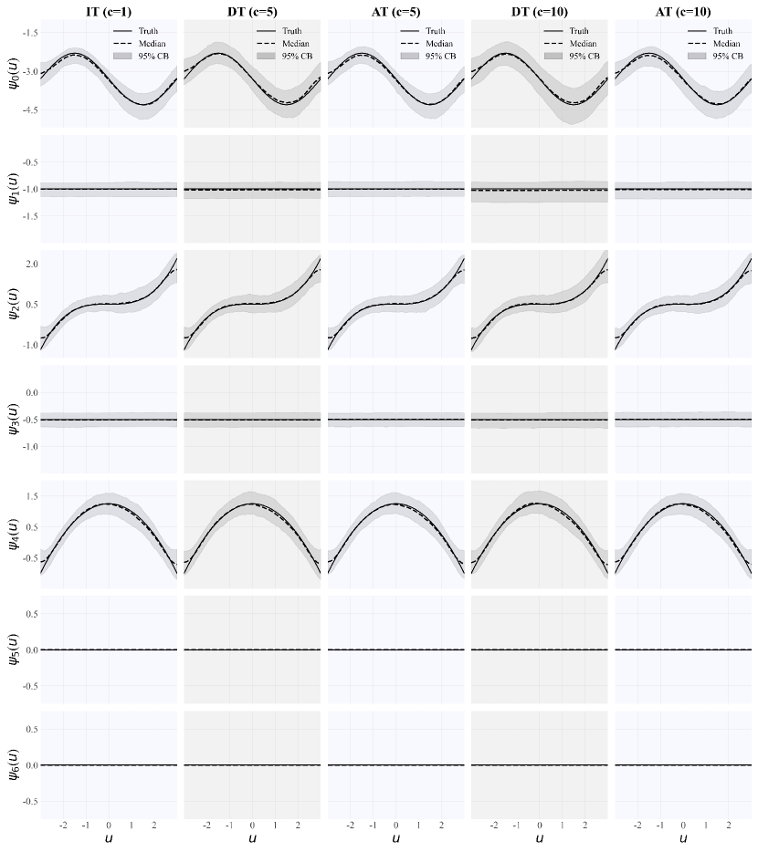
Figure 1: Simulation results for model M1 with sample size $N=5000$, $c\in\{5,10\}$ under both DT and AT protocols. Each subfigure features a solid curve for the true value of the varying coefficient (Truth), a dashed curve for the pointwise median of the $500$ posterior median estimates (Median), and a gray-shaded area for the equal-tailed 95% credible band (95% CB) with the lower and upper bounds being the 2.5% and 97.5% pointwise quantiles of the $500$ posterior median estimates. Results for IT are also presented as a reference.

Table 1 first summarizes the performance of our SSVS process. For evaluation, we consider the inclusion probability (IP) of the $d$th covariate; i.e., $\text{Pr}(\delta_{1d}=1)$. Since $\delta_{2d}$ is binary, this probability can be written as the summation of two: (i) IPF, the inclusion probability of the fixed effect $\alpha_{d}$ but not the varying effect $\beta_{d}(u)$, which is $\Pr(\delta_{1d}=1,\delta_{2d}=0)$; (ii) IPV, the inclusion probability of the varying effect $\beta_{d}(u)$, which is $\Pr(\delta_{1d}=1,\delta_{2d}=1)$. We note that IP is the summation of IPF and IPV. All these probabilities can be estimated using the respective posterior means in each simulation. We report the averages of these estimates from our 500 replications in Table 1 for $d>0$.

Table 1: Simulation results for model set M1 with $N=5000$ and $c\in\{5,10\}$ under both DT and AT. Summary statistics include Bias (empirical bias), SSD (standard deviation of the 500 posterior median estimates), ESE (average of the 500 estimates of the posterior standard deviation), CP95 (empirical coverage probability of equal-tail 95% credible intervals), AVGtest (average number of tests used), and savings (percentage reduction in average number of tests compared to IT). For the performance of the SSVS, inclusion probabilities (IP, IPF, and IPV) are displayed (see Section 5.2 for their definitions).

				$c=5$			$c=10$
Parameter	Summary	IT		DT	AT		DT	AT
$\psi_{5}(u)=0$	IP	0.007		0.007	0.007		0.007	0.007
$\psi_{6}(u)=0$	IP	0.007		0.007	0.008		0.007	0.007
$\psi_{1}(u)=-1.0$	IPF/IPV	0.994/0.005		0.993/0.007	0.993/0.007		0.993/0.007	0.993/0.007
$\psi_{3}(u)=-0.5$	IPF/IPV	0.993/0.007		0.993/0.007	0.994/0.006		0.987/0.014	0.989/0.011
$\delta_{12}=1,\delta_{22}=1$	IPF/IPV	0.000/1.000		0.000/1.000	0.000/1.000		0.000/1.000	0.000/1.000
$\delta_{14}=1,\delta_{24}=1$	IPF/IPV	0.000/1.000		0.000/1.000	0.000/1.000		0.000/1.000	0.000/1.000
$\psi_{1}(u)=\alpha_{1}=-1.0$	Bias(CP95)	-0.008(0.962)		-0.015(0.940)	-0.004(0.942)		-0.034(0.912)	-0.013(0.932)
	SSD(ESE)	0.066(0.069)		0.072(0.072)	0.068(0.067)		0.095(0.083)	0.077(0.074)
$\psi_{3}(u)=\alpha_{3}=-0.5$	Bias(CP95)	-0.007(0.942)		-0.008(0.936)	-0.002(0.938)		-0.012(0.938)	-0.001(0.938)
	SSD(ESE)	0.064(0.063)		0.067(0.063)	0.067(0.062)		0.072(0.068)	0.066(0.065)
$\sigma=0.5$	Bias(CP95)	0.047(0.950)		0.044(0.952)	0.039(0.964)		0.059(0.924)	0.048(0.960)
	SSD(ESE)	0.062(0.079)		0.062(0.080)	0.058(0.078)		0.067(0.084)	0.062(0.081)
$S_{e(1)}=0.95$	Bias(CP95)			-0.032(0.902)	0.000(0.954)		-0.038(0.914)	0.002(0.964)
	SSD(ESE)			0.081(0.053)	0.024(0.021)		0.084(0.062)	0.041(0.034)
$S_{e(2)}=0.98$	Bias(CP95)			-0.008(0.974)	-0.001(0.988)		-0.019(0.972)	-0.006(0.996)
	SSD(ESE)			0.021(0.024)	0.016(0.017)		0.050(0.046)	0.021(0.033)
$S_{p(1)}=0.98$	Bias(CP95)			0.002(0.990)	0.000(0.920)		-0.014(0.992)	-0.010(0.990)
	SSD(ESE)			0.011(0.014)	0.012(0.011)		0.032(0.052)	0.027(0.033)
$S_{p(2)}=0.99$	Bias(CP95)			0.000(0.966)	-0.003(0.974)		-0.003(0.922)	-0.003(0.966)
	SSD(ESE)			0.008(0.007)	0.012(0.013)		0.011(0.009)	0.012(0.011)
Cost	AVGtest(savings)	5000.00(00.00%)		2943.15(41.14%)	2971.33(40.57%)		3567.84(28.64%)	2943.73(41.12%)

When $\psi_{d}(\cdot)=0$, the $d$th covariate is insignificant to the model, meaning $\Pr(\delta_{1d}=1)=0$. Hence, IP should be close to $0$, as evident in Table 1 for $d\in\{5,6\}$. Conversely, when $\psi_{d}(\cdot)\neq 0$, we have two cases: (i) significant but age-independent as $\psi_{d}(u)=\alpha_{d}$, where IPF should be close to $1$ while IPV approaches $0$; (ii) significant and age-varying as $\psi_{d}(u)=\alpha_{d}+\beta_{d}(u)$, where IPF should be close to $0$ while IPV approaches $1$. In Table 1, these patterns are evident for $d\in\{1,3\}$ and $d\in\{2,4\}$, underscoring the effectiveness of our SSVS approach.

For $d\in\{1,3\}$, it’s notable that $\psi_{d}(u)$ reduces to a single value $\alpha_{d}$ . In addition to $\sigma$, $S_{e(m)}$’s, and $S_{p(m)}$’s, Table 1 summarizes our estimates of these parameters across all considered testing protocols. However, we lack results for estimating $S_{e(m)}$’s and $S_{p(m)}$’s under IT since they are not identifiable in this scenario. Examination of these summary statistics reveals minimal to no bias in the estimates, close agreement between SSDs and ESEs, and mostly nominal CP95s. These observations further underscore the inferential capabilities of our method.

Finally, we’d like to discuss the testing protocols. The last row of Table 1 indicates that both DT and AT achieve significant cost reductions (28%–41%) compared to IT, without sacrificing estimation accuracy as both DT and AT protocols at $c=5$ or $c=10$ exhibit minimal variability and comparable estimation performance to IT. These trends are also evident in the results presented in Web Appendix C. In conclusion, our comprehensive simulation study demonstrates that the proposed group testing method is capable of identifying significant age-independent, significant age-varying, and insignificant covariates while achieving comparable performance to IT of adeptly capturing nonlinear patterns and accurately estimating other model parameters but with great cost-savings.

6 Application

We now apply our method to the SHL chlamydia dataset. This data was obtained from screening $N=13862$ females over $L=64$ clinics throughout Iowa in 2014. The screening involved both individual testing and group testing. The individual testing was conducted on all $4316$ urine specimens and $416$ swab specimens. The remaining $9130$ swabs were tested in pools following the DT algorithm. In the group testing part, it tested $2286$ swab master pools ($2273$ pools of size $4$, $12$ of size $3$, and $1$ of size $2$) with additional retests in resolving positive pools.

In addition to all the testing outcomes, the dataset also contains covariates for each participant, denoted by $u_{i}$ and $\mbox{$\hbox{\hbox to0.25pt{$x$\hss}\hbox to0.25pt{$x$\hss}\hbox{$x$}}$}_{i}=(x_{i1},x_{i2},x_{i3},x_{i4},x_{i5},x_{i6},x_{i7},x_{i8})^{\top}$ for $i=1,\dots,N$. Specifically, $u_{i}$ denotes the $i$th female’s age and all $x_{id}$’s are binary: $x_{i1}=1$ for Caucasian participants (and 0 otherwise), $x_{i2}=1$ if a new sexual partner was reported in the last 90 days (and 0 otherwise), $x_{i3}=1$ if multiple partners were reported in the last 90 days (and 0 otherwise), $x_{i4}=1$ if the subject had contact with a partner reporting any STD in the previous year (and 0 otherwise), $x_{i5}=1$ if the patient experienced symptoms of infection such as painful urination/intercourse (and 0 otherwise), $x_{i6}=1$ the female experienced symptoms associated with a friable cervix such as painful intercourse or frequent spotting (and 0 otherwise), $x_{i7}=1$ if the subject experienced the cervicitis, the inflammation of the cervix (and 0 otherwise), and $x_{i8}=1$ if the patient has been diagnosed with the pelvic inflammatory disease (PID), an infection of the female reproductive organs (and 0 otherwise).

To explore whether the association between the $p=8$ covariates (especially race) and chlamydia infection risk varies with age, we fit the following model,

$$\hbox{logit}\left\{\hbox{Pr}\left(\widetilde{Y}_{i}=1\mid u_{i},\mbox{$\hbox{\hbox to0.25pt{$x$\hss}\hbox to0.25pt{$x$\hss}\hbox{$x$}}$}_{i}\right)\right\}= \psi_{0}(u_{i})+\sum_{d=1}^{8}x_{id}\delta_{1d}\{\alpha_{d}+\delta_{2d}\beta_{d}(u_{i})\}+\sum_{\ell=1}^{L}r_{\ell}(i)\gamma_{\ell},$$

for $i=1,2,\ldots,N$, where $Y_{i}$ is the $i$th female’s true (latent) infection status, $\psi_{0}(\cdot)=\alpha_{0}+\beta_{0}(\cdot)$ captures the main age-varying effect (or the intercept term), and for $d>0$, $\delta_{1d}\{\alpha_{d}+\delta_{2d}\beta_{d}(\cdot)\}=\psi_{d}(\cdot)$ depicts the $d$th covariate’s age-varying effect with $(\delta_{1d},\delta_{2d})$ classifying $\psi_{d}(\cdot)$ as either significant age-independent, significant age-varying, or insignificant. The random effects $\gamma_{\ell}$’s follow $\mathcal{N}(0,\sigma^{2})$ independently and account for possible spatial heterogeneity across the $64$ clinic sites, and $r_{\ell}(i)=1$ if $i$th individual specimen was collected at the $\ell$th clinic.

In our model fitting, different sensitivity and specificity parameters are used to account for the testing errors on different specimens. More specifically, we denote by $S_{e(1)}$ and $S_{p(1)}$, respectively, the sensitivity and specificity of the test on the individual swab specimens. For the individual test on the urine specimens, they are denoted by $S_{e(2)}$ and $S_{p(2)}$, and for the test on pooled swab specimens, we use $S_{e(3)}$ and $S_{p(3)}$. This formulation accounts for nuances in assay performance, considering the differences between urine and swab specimens and the distinction between individual and pooled tests. In our analysis, all prior specifications are aligned with those detailed in Section 3. For comparison, we also fit the model without our SSVS process; i.e,

$$\hbox{logit}\left\{\hbox{Pr}\left(\widetilde{Y}_{i}=1\mid u_{i},\mbox{$\hbox{\hbox to0.25pt{$x$\hss}\hbox to0.25pt{$x$\hss}\hbox{$x$}}$}_{i}\right)\right\}= \psi_{0}(u_{i})+\sum_{d=1}^{8}x_{id}\psi_{d}(u_{i})+\sum_{\ell=1}^{L}r_{\ell}(i)\gamma_{\ell}.$$

In the posterior sampling of both models, we discarded the first 5000 draws for MCMC convergence and retained every 50th sample from the subsequent 20000 iterations.

The posterior mean estimate of the standard deviation, $\sigma$, of the random effect is $0.426$ with a 95% highest posterior density (HPD) credible interval of $(0.313,0.545)$. This indicates that the random effect is strongly significant, providing clear evidence of heterogeneity across clinics statewide. This result reinforces earlier findings from Chen et al. (2009) and Joyner et al. (2020). Regarding the six assay accuracy probabilities, our findings align with those reported in McMahan et al. (2017) and Liu et al. (2021) and are thus presented in Web Table S.4 in Web Appendix D.

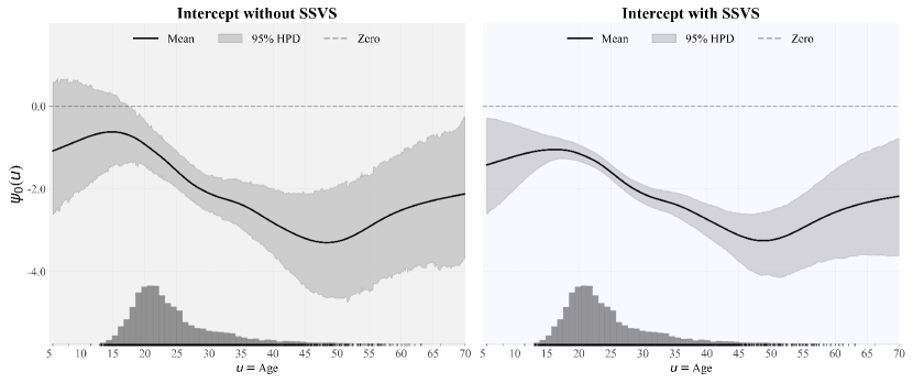
Figure 2: Iowa chlamydia data: the main age effect. Each subfigure displays the pointwise posterior mean (Mean) estimates and the pointwise 95% HPD credible band (95% HPD). The zero reference line is dashed. All the females’ ages are plotted in dots and summarized in a (rescaled) histogram on the age-axis.

We now turn our attention to the regression coefficients. We start with the estimates of the main age effect $\psi_{0}(u)$ that are summarized in Figure 2. The left and right panels present estimates of $\psi_{0}(u)$ without and with SSVS, respectively. Therein, solid lines depict the pointwise posterior mean estimates of the curve, while shaded areas represent the pointwise 95% HPD credible bands. The age-axis has the ages of all female individuals as dots, accompanied by a (rescaled) histogram illustrating the distribution of these ages. Upon comparison, it becomes evident that although our SSVS regularizes the other covariates, it still benefits the estimate of $\psi_{0}(u)$. Notably, the credible band on the right is much narrower than that on the left, highlighting the non-linear trend in the estimates of $\psi_{0}(u)$. It’s worth mentioning that this non-linear pattern is similar to the one identified by the generalized partially linear additive model in Liu et al. (2021), which highlights a peak in infection risk around the age of 18, alongside a noticeable rise in risk for individuals aged 50 and above. We acknowledge that the non-linear patterns observed in the age groups 5–13 and 45–70 offer less informative insights compared to the age range 13–45, likely due to the limited availability of data near those boundaries, a phenomenon commonly known as the boundary effect in nonparametric estimation. The peak around 18 is more informative and aligns closely with CDC screening recommendations for chlamydia in sexually active females aged 24 or younger (CDC, 2021).

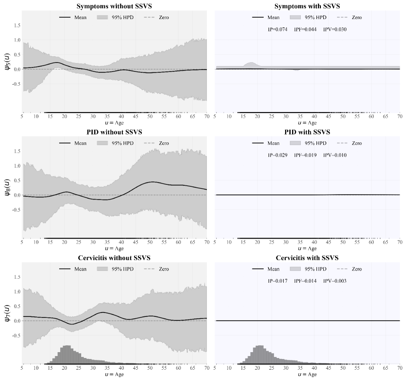
Figure 3: Iowa chlamydia data: insignificant covariates. Each subfigure displays the pointwise posterior mean (Mean) estimates and the pointwise 95% HPD credible band (95% HPD). The zero reference line is dashed. All the females’ ages are plotted in dots and summarized in a (rescaled) histogram on the bottom age-axis. With SSVS, the estimated IP, IPF, and IPV are also provided.

For covariates, $x_{1},\dots,x_{8}$, we categorize them into three groups based on the SSVS outputs. Those with an estimated $\mbox{IP}\leq 0.1$ are considered insignificant covariates. We choose $0.1$ as the threshold for two reasons: (1) it’s a commonly used significance level in standard statistical hypothesis testing, and (2) we would rather be a bit conservative than overlook any significant covariates. Based on this criteria, the insignificant covariates identified are $x_{5}$, $x_{7}$, and $x_{8}$, with IPs of $0.074$, $0.017$, and $0.029$, respectively. Figure 3 provides a summary of these estimates. In the case of $\psi_{7}(\cdot)$ and $\psi_{8}(\cdot)$, the figures on the left (without SSVS) present non-linear estimates but with a wide 95% HPD credible band covering zero across all ages. Unsurprisingly, SSVS regularization precisely sets them to zero. In the corresponding figures, both the posterior mean estimate and the 95% HPD credible intervals have been unified to the zero horizontal line, providing compelling evidence that PID or cervicitis does not significantly associate with chlamydia infection risk. Similarly, $x_{5}$ (symptoms) is also deemed insignificant, indicating that the presence of symptoms does not impact the risk of chlamydia infection. This aligns with expectations, as chlamydia infections frequently occur without symptoms yet can still attack a woman’s reproductive system. Moreover, the SSVS credible band of $\psi_{5}(u)$ becomes slightly larger between ages 15 and 22 compared to other age groups, likely due to this age range being the most vulnerable period to chlamydia.

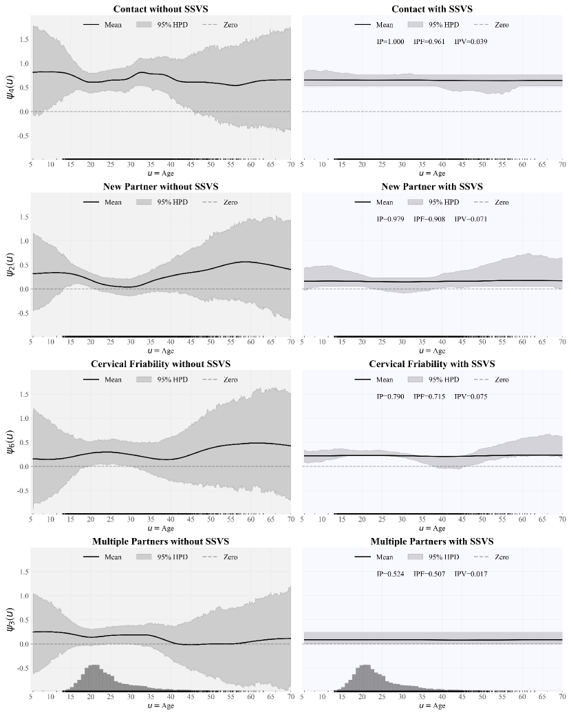
Figure 4: Iowa chlamydia data: significant and age-independent covariates. Each subfigure displays the pointwise posterior mean (Mean) estimates and the pointwise 95% HPD credible band (95% HPD). The zero reference line is dashed. All the females’ ages are plotted in dots and summarized in a (rescaled) histogram on the bottom age-axis. With SSVS, the estimated IP, IPF, and IPV are also provided.

Those covariates with estimated $\mbox{IP}>0.1$ and $\mbox{IPV}\leq 0.1$ are considered significant age-independent. This category includes $x_{2}$, $x_{3}$, $x_{4}$, $x_{6}$, with $\mbox{IP}=0.979,0.524,1.000,0.979$ and $\mbox{IPV}=0.071,0.017,0.039,0.075$, respectively. The corresponding estimates are summarized in Figure 4. Again, employing SSVS results in substantially narrower credible bands compared to analyses without SSVS. All posterior mean estimates, with a majority of their credible bands, remain above zero, suggesting that chlamydia risk escalates with factors such as having contact with STDs ($x_{2}=1$), acquiring a new sexual partner ($x_{3}=1$), engaging in multiple partnerships ($x_{4}=1$), or experiencing a friable cervix ($x_{4}=1$). This finding aligns with known epidemiological trends of chlamydia (LeFevre and USPSTF, 2014).

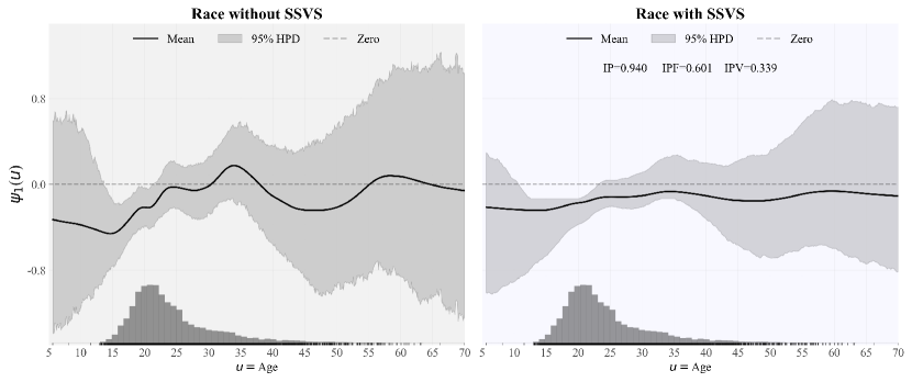
Figure 5: Iowa chlamydia data: the significant and age-varying covariate. Each subfigure displays the pointwise posterior mean (Mean) estimates and the pointwise 95% HPD credible band (95% HPD). The zero reference line is dashed. All the females’ ages are plotted in dots and summarized in a (rescaled) histogram on the bottom age-axis. With SSVS, the estimated IP, IPF, and IPV are also provided.

Covariates exhibiting estimated $\mbox{IP}>0.1$ and $\mbox{IPV}>0.1$ are considered significant age-varying. In this analysis, only race ($x_{1}$) falls into this category, with $\mbox{IP}=0.94$ and $\mbox{IPV}=0.339$. With the implementation of SSVS, the posterior mean estimate of $\psi_{1}(u)$ displays reduced fluctuation along with a narrower credible interval in Figure 5 as expected. A particularly intriguing discovery emerges within the age bracket of 11 to 23. Within this range, there are 7571 females, constituting approximately 54.6% of the sample size, and the SSVS estimate of $\psi_{1}(u)$, along with its credible band, is consistently negative throughout this span. This suggests that individuals who are non-Caucasian ($x_{1}=0$) between the ages of 11 and 23 exhibit greater vulnerability compared to people who are Caucasian ($x_{1}=1$), with this discrepancy gradually diminishing after age $25$. This finding closely aligns with results reported in Chambers et al. (2018). We believe that this finding not only highlights the crucial need for utilizing varying-coefficient models when analyzing group testing data but also prompts policymakers to consider the age-varying racial disparity in developing interventions and prevention strategies for better chlamydia control and management.

7 Discussion

This article introduces a Bayesian varying-coefficient model tailored for group testing data, enabling regression coefficients to vary with a chosen covariate, estimating unknown test accuracies, and providing an option for integrating spatial random effects. The model utilizes GPP prior distribution to estimate these varying coefficients. To ensure informative inference, we employ the SSVS process for regularization and categorize covariates into three groups. Through careful data augmentation, we develop a computationally efficient posterior sampling algorithm. Simulation results consistently demonstrate the method’s effectiveness in estimating regression parameters and performing variable selection. These techniques are applied to analyze SHL group testing data from Iowa’s chlamydia screening, revealing an intriguing age-varying pattern in the racial disparity of the disease.

As previously discussed in Liu et al. (2021), it’s important to acknowledge that the chlamydia dataset analyzed here wasn’t obtained from a random sample of Iowa females. Rather, it may be considered representative of the “highest-risk” residents. This aspect should be taken into account when interpreting the outcomes of our data analysis. However, this characteristic neither undermines the significance of our study’s contribution nor restricts the applicability of our method to a random sample if one is available.

Future directions within this research line involve exploring more flexible approaches to modeling the varying coefficients. For instance, one could expand upon Bayesian additive regression trees (BART) (Chipman et al., 2010) to estimate these coefficients. BART offers greater flexibility compared to GPP priors, allowing for the capture of discontinuously varying functions and automatic determination of covariate importance for variable selection. Another possibility is to use Dirichlet processes (DP) (Gelfand et al., 2005; Cai et al., 2013) for age-varying coefficients, alleviating biases associated with the normality assumption of age-varying coefficients inherent in GPP. Furthermore, one could explore the development of a multivariate varying coefficient model (Reich et al., 2010; Zhu et al., 2012), in which, each coefficient is a function of both age and race, facilitating more flexibility in understanding racial disparities. Regarding testing accuracies, another avenue for investigation could be to address the dilution effect in testing errors, where testing sensitivity might decrease when pooling a positive specimen with multiple negative ones. Previous work by Wang et al. (2015) may provide valuable insights in this regard. Lastly, there is potential to extend this work by developing joint varying-coefficient modeling methods that incorporate testing responses from multiplex assays. These assays, which test for multiple diseases simultaneously, have gained popularity among many public health labs.

Funding

This research was supported by National Institutes of Health grants R03-AI135614 and R01-AI121351.

Supplementary Materials

Web Appendices A–D, referenced in Sections 3–6, are available with the submission. The R code and documentation for simulation are publicly available at the GitHub repository: https://github.com/yizenglistat/rvcm4gt.

References

- Banerjee et al. (2008) Banerjee, S., Gelfand, A. E., Finley, A. O., and Sang, H. (2008). Gaussian predictive process models for large spatial data sets. Journal of the Royal Statistical Society: Series B (Statistical Methodology) 70, 825–848.
- Bergquist et al. (2019) Bergquist, E. P., Trolard, A., Fox, B., Kuhlmann, A. S., Loux, T., Liang, S. Y., Stoner, B. P., and Reno, H. (2019). Presenting to the emergency department versus clinic-based sexually transmitted disease care locations for testing for chlamydia and gonorrhea: A spatial exploration. Sexually transmitted diseases 46, 474–479.
- Bilder and Tebbs (2009) Bilder, C. R. and Tebbs, J. M. (2009). Bias, efficiency, and agreement for group-testing regression models. Journal of statistical computation and simulation 79, 67–80.
- Cai et al. (2013) Cai, B., Lawson, A. B., Hossain, M. M., Choi, J., Kirby, R. S., and Liu, J. (2013). Bayesian semiparametric model with spatially–temporally varying coefficients selection. Statistics in medicine 32, 3670–3685.
- CDC (2021) CDC (2021). Sexually Transmitted Disease Surveillance, Centers for Disease Control and Prevention 2021. https://www.cdc.gov/std/statistics/2020/2020-SR-4-10-2023.pdf. [Accessed 26-02-2024].
- Chambers et al. (2018) Chambers, L. C., Khosropour, C. M., Katz, D. A., Dombrowski, J. C., Manhart, L. E., and Golden, M. R. (2018). Racial/ethnic disparities in the lifetime risk of chlamydia trachomatis diagnosis and adverse reproductive health outcomes among women in king county, washington. Clinical Infectious Diseases 67, 593–599.
- Chen et al. (2009) Chen, P., Tebbs, J. M., and Bilder, C. R. (2009). Group testing regression models with fixed and random effects. Biometrics 65, 1270–1278.
- Chipman et al. (2010) Chipman, H. A., George, E. I., and McCulloch, R. E. (2010). Bart: Bayesian additive regression trees. The Annals of Applied Statistics 4,.
- Cleveland et al. (1992) Cleveland, W. S., Grosse, E., Shyu, W. M., Chambers, J. M., and Hastie, T. J. (1992). Statistical models in s. Local regression models pages Chapter–8.
- Delaigle et al. (2014) Delaigle, A., Hall, P., and Wishart, J. (2014). New approaches to nonparametric and semiparametric regression for univariate and multivariate group testing data. Biometrika 101, 567–585.
- Delaigle and Meister (2011) Delaigle, A. and Meister, A. (2011). Nonparametric regression analysis for group testing data. Journal of the American Statistical Association 106, 640–650.
- Dorfman (1943) Dorfman, R. (1943). The detection of defective members of large populations. The Annals of Mathematical Statistics 14, 436–440.
- Gelfand et al. (2005) Gelfand, A. E., Kottas, A., and MacEachern, S. N. (2005). Bayesian nonparametric spatial modeling with dirichlet process mixing. Journal of the American Statistical Association 100, 1021–1035.
- Gelman (2009) Gelman, A. (2009). Bayes, jeffreys, prior distributions and the philosophy of statistics. Statistical Science 24, 176–178.
- Gneiting et al. (2010) Gneiting, T., Kleiber, W., and Schlather, M. (2010). Matérn cross-covariance functions for multivariate random fields. Journal of the American Statistical Association 105, 1167–1177.
- Gregory et al. (2019) Gregory, K. B., Wang, D., and McMahan, C. S. (2019). Adaptive elastic net for group testing. Biometrics 75, 13–23.
- Hastie and Tibshirani (1993) Hastie, T. and Tibshirani, R. (1993). Varying-coefficient models. Journal of the Royal Statistical Society: Series B (Methodological) 55, 757–779.
- Huang (2009) Huang, X. (2009). An improved test of latent-variable model misspecification in structural measurement error models for group testing data. Statistics in medicine 28, 3316–3327.
- Joyner et al. (2020) Joyner, C. N., McMahan, C. S., Tebbs, J. M., and Bilder, C. R. (2020). From mixed effects modeling to spike and slab variable selection: A bayesian regression model for group testing data. Biometrics 76, 913–923.
- Kim et al. (2007) Kim, H.-Y., Hudgens, M. G., Dreyfuss, J. M., Westreich, D. J., and Pilcher, C. D. (2007). Comparison of group testing algorithms for case identification in the presence of test error. Biometrics 63, 1152–1163.
- Land et al. (2010) Land, J., Van Bergen, J., Morre, S., and Postma, M. (2010). Epidemiology of chlamydia trachomatis infection in women and the cost-effectiveness of screening. Human reproduction update 16, 189–204.
- LeFevre and USPSTF (2014) LeFevre, M. L. and USPSTF (2014). Screening for chlamydia and gonorrhea: Us preventive services task force recommendation statement. Annals of internal medicine 161, 902–910. US Preventive Services Task Force (USPSTF).
- Lin et al. (2019) Lin, J., Wang, D., and Zheng, Q. (2019). Regression analysis and variable selection for two-stage multiple-infection group testing data. Statistics in medicine 38, 4519–4533.
- Liu et al. (2012) Liu, A., Liu, C., Zhang, Z., and Albert, P. S. (2012). Optimality of group testing in the presence of misclassification. Biometrika 99, 245–251.
- Liu et al. (2021) Liu, Y., McMahan, C. S., Tebbs, J. M., Gallagher, C. M., and Bilder, C. R. (2021). Generalized additive regression for group testing data. Biostatistics 22, 873–889.
- McMahan et al. (2017) McMahan, C. S., Tebbs, J. M., Hanson, T. E., and Bilder, C. R. (2017). Bayesian regression for group testing data. Biometrics 73, 1443–1452.
- Phatarfod and Sudbury (1994) Phatarfod, R. and Sudbury, A. (1994). The use of a square array scheme in blood testing. Statistics in Medicine 13, 2337–2343.
- Polson et al. (2013) Polson, N. G., Scott, J. G., and Windle, J. (2013). Bayesian inference for logistic models using pólya–gamma latent variables. Journal of the American statistical Association 108, 1339–1349.
- Reich et al. (2010) Reich, B. J., Fuentes, M., Herring, A. H., and Evenson, K. R. (2010). Bayesian variable selection for multivariate spatially varying coefficient regression. Biometrics 66, 772–782.
- Roberts et al. (2006) Roberts, T., Robinson, S., Barton, P., Bryan, S., and Low, N. (2006). Screening for chlamydia trachomatis: a systematic review of the economic evaluations and modelling. Sexually transmitted infections 82, 193.
- Tebbs et al. (2013) Tebbs, J. M., McMahan, C. S., and Bilder, C. R. (2013). Two-stage hierarchical group testing for multiple infections with application to the infertility prevention project. Biometrics 69, 1064–1073.
- Vansteelandt et al. (2000) Vansteelandt, S., Goetghebeur, E., and Verstraeten, T. (2000). Regression models for disease prevalence with diagnostic tests on pools of serum samples. Biometrics 56, 1126–1133.
- Wang et al. (2014) Wang, D., McMahan, C., Gallagher, C., and Kulasekera, K. (2014). Semiparametric group testing regression models. Biometrika 101, 587–598.
- Wang et al. (2015) Wang, D., McMahan, C. S., and Gallagher, C. M. (2015). A general regression framework for group testing data, which incorporates pool dilution effects. Statistics in medicine 34, 3606–3621.
- Wang et al. (2013) Wang, D., Zhou, H., and Kulasekera, K. (2013). A semi-local likelihood regression estimator of the proportion based on group testing data. Journal of Nonparametric Statistics 25, 209–221.
- Workowski (2013) Workowski, K. (2013). Chlamydia and gonorrhea. Annals of internal medicine 158, ITC2–1.
- Xie (2001) Xie, M. (2001). Regression analysis of group testing samples. Statistics in medicine 20, 1957–1969.
- Zhu et al. (2012) Zhu, H., Li, R., and Kong, L. (2012). Multivariate varying coefficient model for functional responses. Annals of statistics 40, 2634.