Prompt-prompted Mixture of Experts
for Efficient LLM Generation
Abstract
With the development of transformer-based large language models (LLMs), they have been applied to many fields due to their remarkable utility, but this comes at a considerable computational cost at deployment. Fortunately, some methods such as pruning or constructing a mixture of experts (MoE) aim at exploiting sparsity in transformer feedforward (FF) blocks to gain boosts in speed and reduction in memory requirements. However, these techniques can be very costly and inflexible in practice, as they often require training or are restricted to specific types of architectures. To address this, we introduce GRIFFIN, a novel training-free MoE that selects unique FF experts at the sequence level for efficient generation across a plethora of LLMs with different non-ReLU activation functions. This is possible due to a critical observation that many trained LLMs naturally produce highly structured FF activation patterns within a sequence, which we call flocking. Despite our method’s simplicity, we show with 50% of the FF parameters, GRIFFIN maintains the original model’s performance with little to no degradation on a variety of classification and generation tasks, all while improving latency (e.g. 1.25 speed-up in Llama 2 13B on an NVIDIA L40). Code is available at https://github.com/hdong920/GRIFFIN.
1 Introduction
Transformers [VSP+17] have demonstrated incredible capabilities across a plethora of domains [LWLQ22, KNH+22, NBZ+23]. Their large language model (LLM) successors [TMS+23, TAB+23, JSM+23, JSR+24, TMH+24, Ant24] have pushed the bar higher, but these behemoths have become performative at the price of enormous amounts of computation and memory demands. One significant contributor is the model size itself. Not only is storage an issue, model layers tend to be wide and plenty, slowing down inference. Moreover, given the existence of sparse structures in LLMs, especially in feedforward (FF) blocks [GSBL20, DLBZ22, LYB+22, LWD+23], these models waste computation on intermediate features with little to no impact on the final result. For instance, it has been observed that in OPT-175B [ZRG+22], fewer than 5% of neurons in FF blocks have nonzero values per token [LWD+23], meaning 95% of the compute in each FF block is wasted. Usually consisting of around two-thirds of the parameters in an LLM, FF blocks can be serious memory and compute bottlenecks. These inefficiencies are highly problematic in latency-sensitive scenarios like in chatbots and autonomous vehicles.
There have been many methods to exploit sparsity in LLMs for efficiency gains, such as pruning model weights and constructing mixtures of experts (MoEs). Pruning removes low-impact pre-trained weights to reduce storage, yet this often does not translate to real speed-ups in practice, unless the pruning is done in a hardware-friendly manner which typically causes greater performance deterioration. MoEs better preserve the original performance by adaptively selecting subsets of the model to use per input but also come with drawbacks. Unless the model has been trained in this fashion [FZS22, JSR+24], it will need to learn a cheap yet effective gating function (expert selection mechanism) and sometimes even require full fine tuning. Perhaps an even bigger weakness of many of these methods is the inability to effectively carry over to pre-trained LLMs with non-ReLU activations. We seek to overcome these challenges with MoEs:
-
1.
Most current LLMs are not MoEs, so they must be adapted by training gating functions and/or fine tuning the whole model.
-
2.
Gating functions should be simple enough to not cost more than they save.
-
3.
Many current approaches work solely on FF blocks with ReLUs or depend on expensive conversions to ReLUs.
Daunting at first, these challenges become surmountable because of a simple observation of a phenomenon we call flocking, highly consistent sparse activations that persist throughout a sequence observed in many LLMs. Flocking emerges in FF activations (inputs into the FF down projection) when we focus on a sequence’s relative activation magnitudes instead of the absolute values. Examples from Llama 2 7B and Gemma 7B are shown in Figure 1. The key takeaway is that neurons which produce high relative magnitudes are naturally shared across tokens within a sequence, as seen with the distinct vertical streaks. Increasingly bizarre, the two models have different architectures and different non-ReLU activation functions.


Unlike existing pruning or MoE methods, we exploit flocking in our design of GRIFFIN (Gating by Repetition In Feedforward Intermediate Neurons), a highly performative and efficient training-free method to turn an LLM into an MoE. GRIFFIN does this by using a sequence’s prompt to determine the experts to activate during generation, allowing it to overcome all of the aforementioned challenges:
-
1.
No Preparation: Our no-cost method is completely training-free and requires no preparation. Moreover, the simple implementation of GRIFFIN means it can easily be dropped into any FF block.
-
2.
Simple Expert Selection: Since flocking exists throughout a sequence, the prompt reveals the most relevant FF neurons for generation with little to no performance loss. The selection process is parameter-free and adds negligible overhead.
-
3.
Model & Activation Function Diversity: Thorough experimentation demonstrates the efficacy of GRIFFIN on numerous models, including Llama 2 [TMS+23], Gemma [TMH+24], Mistral [JSM+23], OPT [ZRG+22], and ReluLlama [Tea23]. Together, the tested activation functions include ReLU, SwiGLU, GEGLU, and ReGLU [Sha20].
In this paper, we show GRIFFIN is a simple and strong method to turn any LLM into MoE because of flocking. In the next section (Section 2), we discuss some strengths and weaknesses of current methods that seek to improve FF efficiency. In more detail, we formalize the MoE problem and its motivation in Section 3 and present our novel approach in Section 4.2, which requires a thorough examination of the surprising phenomenon of flocking shared by many LLMs in Section 4.1. Our rigorous experiments demonstrate GRIFFIN preserves performance on classification and generation even after removing 50% of FF neurons (Section 5.1), all while having lower latency (Section 5.2). For instance, GRIFFIN reduces the number of active parameters in Llama 2 13B from 13B to 8.8B during generation to improve latency by 1.25 with almost no loss in performance. Finally, we show our method’s incredible scalability and robustness in several ablation studies (Section 5.3).
2 Background
Our novel method and FF activation observations are inspired and motivated by ample amounts of previous research that sought to characterize FF sparsity and accelerate LLMs.
Feedforward Activation Sparsity.
The observation that transformer FF blocks produce sparse activations is not new [GSBL20, DLBZ22, LYB+22, DCC23, LWD+23]. In ReLU-based LLMs like OPT [ZRG+22], the activations can be exceptionally sparse and become more apparent for larger models [LWD+23]. As more models use non-sparse activation functions like GLU variants [Sha20], it is difficult for neurons to have no contribution to the output since these functions do not have an interval that maps to zero. Without exact sparsity, the efficacy of these methods becomes limited. As such, this has ushered a wave of models that are either adapted from available models [ZLL+21, LLLC21, MAM+23, ZBC+24, JSR+24] or trained from scratch [FZS22] which can produce activations that are exactly zero with little to no performance loss. Even so, these methods require considerable amounts of computational resources.
Pruning.
Pruning [LDS89] is another sparsity-guided way to tackle compute and memory bottlenecks of models. Previously, the common method would be some variation of iteratively rounding weights down to zero based on some score and retraining to recover any lost performance [FC18, BGOFG20, LGW+21, LZH+24]. While this can result in most parameters being pruned, this method comes with a few issues. First, with the increasing scale of LLMs, retraining becomes impractical for most. Fortunately, cheap methods to effectively prune LLMs have been developed [FA23, SLBK23, JLC+23, DKK+24]. The second issue is that unless pruning is done in a structured manner [XZC22, SWSL23, MFW23, LYZ+23, XGZC23], it is difficult to see real computational savings, yet structured pruning often leads to much more severe performance degradation. Third, pruning enforces sparsity to be static which can be strong assumption since FF blocks are widely believed to contain the model’s memory [GSBL20].
Mixture of Experts.
Making sparsity more dynamic has motivated the design of mixture-of-experts (MoEs) [JJNH91] to avoid computing low-impact features in trained models at varying granularities [ZLL+21, LWD+23, PSBW23, CIS23, AMB+23, YYB+24, ZBC+24]. The main idea of MoEs is to use a gating function to identify a small subset of neurons that will be used to compute the layer’s output, an adaptive form of pruning. In the ideal case, all active neurons are selected and inactive neurons are ignored for each input. However, current methods either require training or rely on ReLU activation functions. Our method has the best of both worlds: it is training-free and effective on a variety of activation functions.
3 Problem Formulation
This section contains an overview of different components of the FF block followed by a more detailed introduction of the MoE problem which our method aims to tackle. Since FF blocks operate identically and independently for each token unlike attention, we begin with defining the FF block with a single column vector input :
| (1) |
where is a linear transformation and is nonlinear. This describes a wide range of FF architectures and arbitrary activation functions . For instance, in OPT,
| (2) |
For FF blocks with GLU variants such as in Llama 2 and Gemma,
| (3) |
where signifies element-wise multiplication. For all examples, and where typically, . We refer to as the FF activations. The goal of MoEs is to find , , and (additionally and if needed) where such that when the FF block is reparameterized with these matrices, the output value is preserved. In other words, for
| (4) | ||||
| (5) |
, and similarly for FF blocks with non-GLU functions. In the MoE setting, these smaller matrices can vary from token to token and are actually selections of rows and columns of the original structures. Crucially, this selection leads to multiplication with smaller matrices which are naturally efficient on GPUs and TPUs [FSH04, WWB19]. For all equations defined in this section, they operate independently on each row of a length sequence input (e.g. the activations for a sequence are ).
4 From Flocking to GRIFFIN
Here, we take deeper dive into the phenomenon of flocking and describe the intuitive algorithm of GRIFFIN which is directly inspired by it.
4.1 Observing Flocking
Flocking arises when we look at the relative impact of each neuron per token within a sequence. To see this, we normalize rows of to be unit vectors to construct (i.e. ), the relative activations. We show example relative activation magnitudes for a sequence in Llama 2 7B and Gemma 7B in Figure 1. Since there are distinct vertical streaks, this intriguingly implies that activations that have relatively greater weight are common across all tokens in a sequence. Notably, Llama 2 7B and Gemma 7B use SwiGLU and GEGLU activations, respectively, along with other major architecture differences. We call this phenomenon flocking, like highly organized groups of birds, and we observe this in virtually all FF layers (see Appendix B).
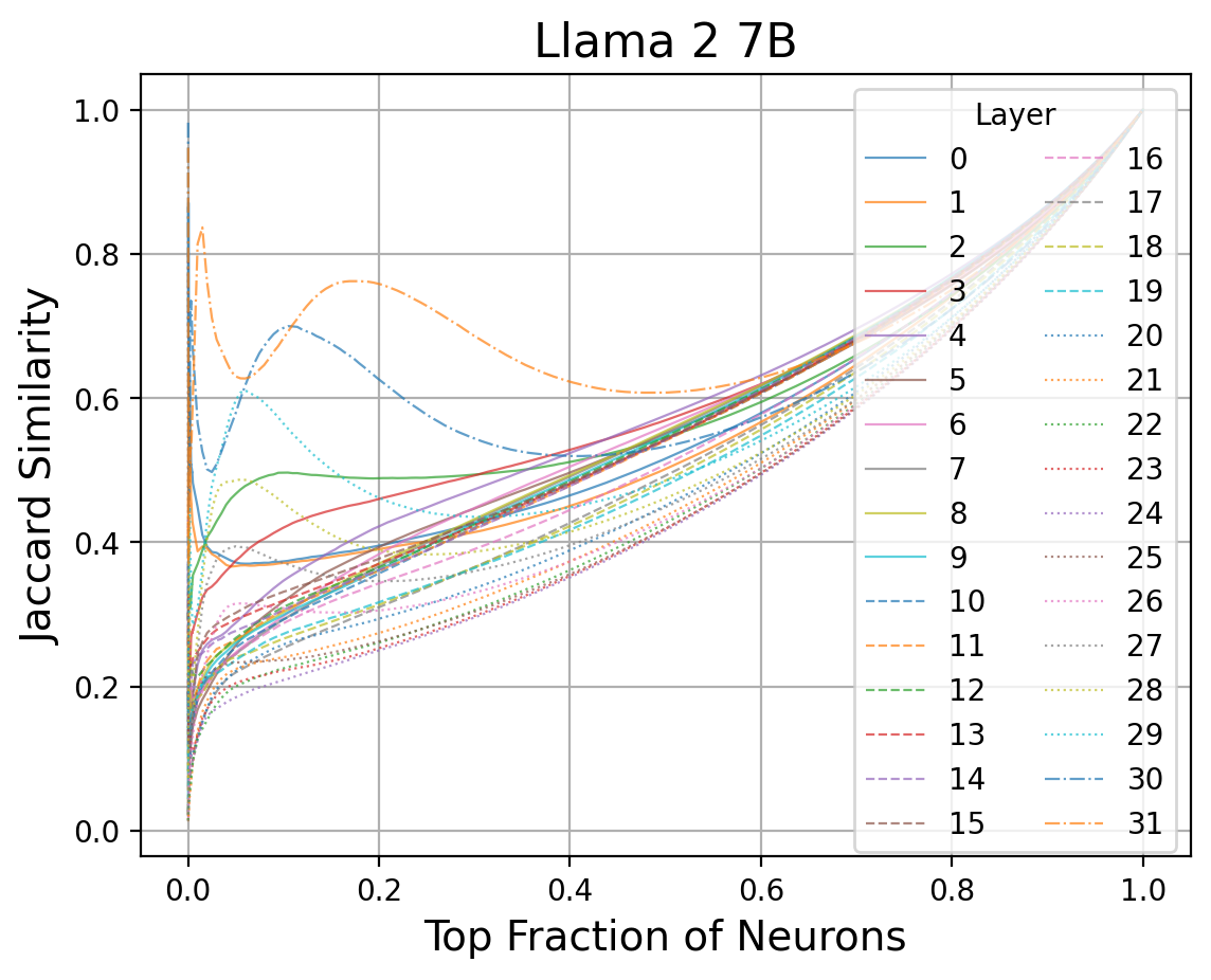
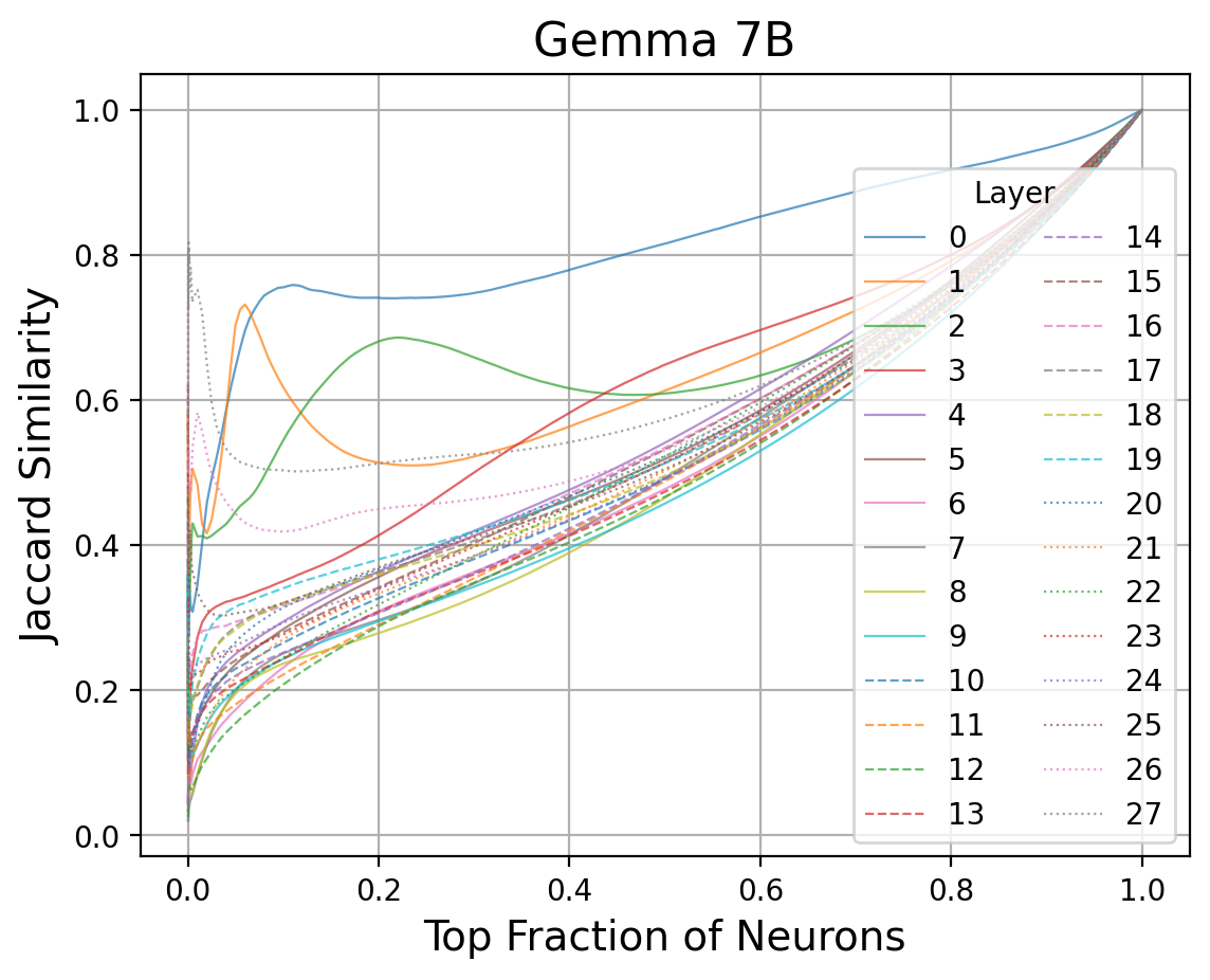
While relative activations magnitudes are shared within a sequence, they are not generally shared between sequences. We show this by taking the -norm of along the token axis to obtain a length vector for each sample or sequence, roughly capturing the contribution of each FF neuron throughout a sequence. Taking the top- of this for each sample at each layer, we find the Jaccard similarity between two sequences based on the indices selected for different . In other words, we compute the intersection over union of every unique pair of top- sets. Higher values indicate more similar top- sets. From Figure 2 where we aggregate Jaccard similarities across WikiText [MXBS16] samples, we observe a lack of inter-sample activation similarities for the vast majority of layers in Llama 2 7B and Gemma 7B, unless the sets of selected neurons are large. This lack of consistency implies pruning entire FF neurons without retraining would be less effective than a more adaptive method.
4.2 GRIFFIN Algorithm
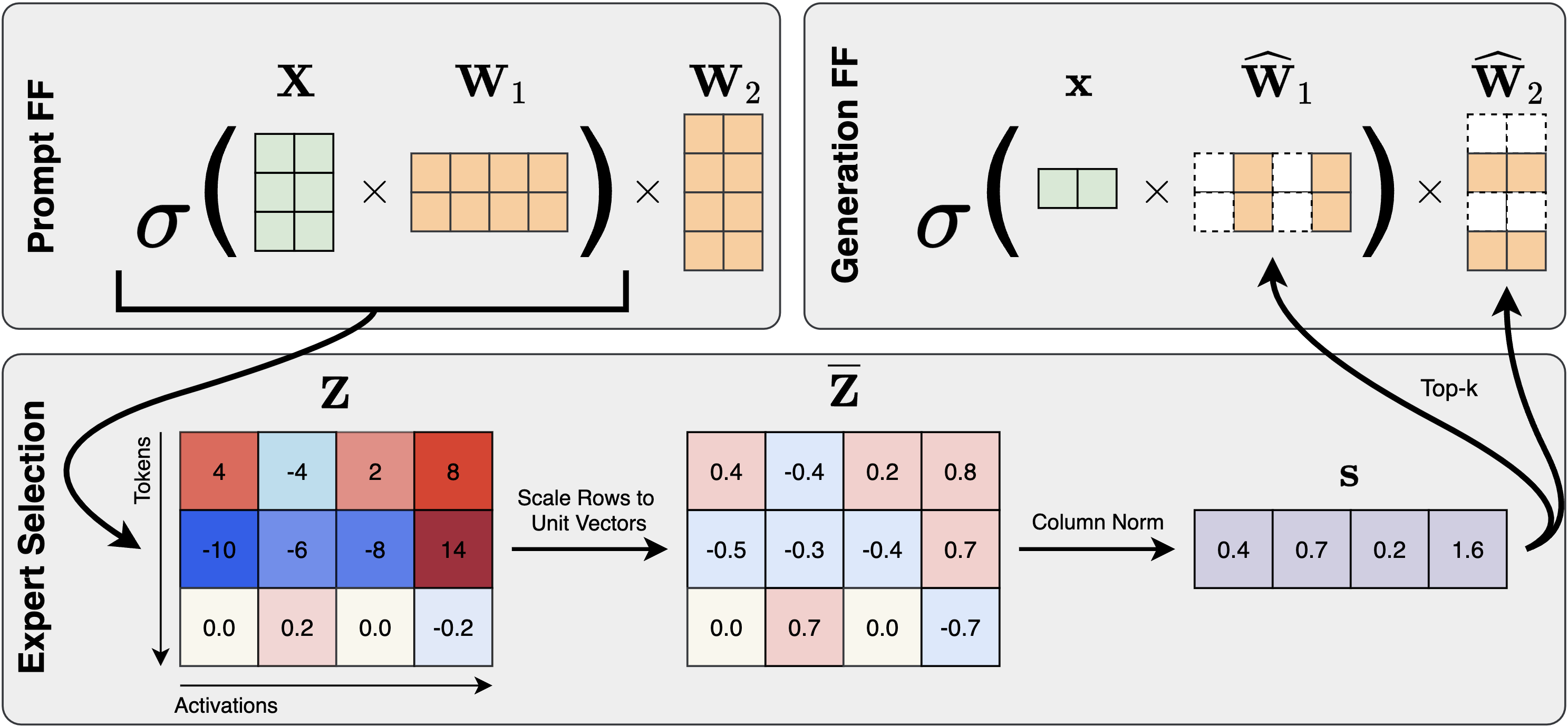
Using our insight on flocking, we introduce GRIFFIN as a simple general purpose and training-free MoE method for efficient generation, captured in Figure 3. In a nutshell, we select experts during the prompt phase of each sample which are then used for the entire duration of the generation phase. This effective approach is based on a key observation on flocking: since tokens within a sequence share activation patterns, the prompt and generated tokens will also share activation patterns.
Prompt Phase Expert Selection.
Our experts or neurons are chosen at the sequence level, so we need to consider the dynamics of the entire input sequence rather than just a single token when choosing our experts. To select expert neurons, we need a statistic to inform us of the importance of each neuron. At the prompt phase, we do this by aggregating taking the -norm of along the token axis:
| (6) |
Taking the indices of the top- across gives us the neurons we will use for this sample’s generation phase which make up the set . Using the experts in , we can find by selecting corresponding rows and columns in , and , respectively. This is done for every FF block during the prompt phase. Elaborated in Appendix A, highlights neurons consistently activated at relatively high intensities.
Generation with Experts.
When generating tokens, we directly use the pruned layers which contain the expert neurons, and , to estimate for all future tokens. In Llama 2 13B and Gemma 7B, this reduces the active number of parameters from 13B to 8.8B and from 8.5B to 5.4B, respectively, during generation.
5 Experiments
We showcase the superb performance of GRIFFIN on numerous tasks and models (Section 5.1) while achieving lower latency (Section 5.2), along with a study on several of its properties like sampling experts, sequence length scaling, and random inputs (Section 5.3). All experiments are run on NVIDIA L40 GPUs.
5.1 Performance
| Model | HellaSwag | PIQA | COPA | ARC-e | ARC-c | BoolQ |
|---|---|---|---|---|---|---|
| Llama 2 7B | 57.16 | 78.07 | 87.00 | 76.35 | 43.34 | 77.71 |
| Magnitude | 57.12 | 77.31 | 84.00 | 70.33 | 40.27 | 66.54 |
| GRIFFIN | 57.11 | 77.69 | 86.00 | 74.54 | 42.75 | 73.15 |
| Llama 2 13B | 60.06 | 79.05 | 90.00 | 79.46 | 48.46 | 80.61 |
| Magnitude | 60.00 | 79.00 | 88.00 | 74.07 | 46.25 | 70.52 |
| GRIFFIN | 60.10 | 79.11 | 89.00 | 77.19 | 46.84 | 78.50 |
| Gemma 7B | 60.61 | 80.30 | 88.00 | 82.74 | 50.09 | 83.49 |
| Magnitude | 46.24 | 73.12 | 57.00 | 45.20 | 32.76 | 62.84 |
| GRIFFIN | 60.62 | 79.98 | 88.00 | 81.65 | 50.09 | 81.90 |
| Mistral 7B | 61.21 | 80.58 | 92.00 | 80.89 | 50.43 | 83.61 |
| Magnitude | 61.15 | 80.36 | 86.00 | 74.20 | 48.89 | 60.40 |
| GRIFFIN | 61.18 | 80.52 | 91.00 | 79.25 | 50.00 | 80.06 |
| OPT 6.7B | 50.48 | 76.28 | 81.00 | 65.53 | 30.55 | 66.12 |
| Magnitude | 49.21 | 72.63 | 79.00 | 47.60 | 27.13 | 40.15 |
| GRIFFIN | 50.44 | 75.63 | 80.00 | 63.93 | 30.55 | 65.44 |
| OPT 13B | 52.46 | 75.90 | 86.00 | 67.05 | 32.94 | 65.81 |
| Magnitude | 51.31 | 74.21 | 81.00 | 49.41 | 28.07 | 38.75 |
| GRIFFIN | 52.42 | 76.17 | 86.00 | 66.92 | 33.19 | 67.65 |
Using various models, we evaluate on several generation and classification tasks. For generation, we evaluate on XSum [NCL18], CNN/DailyMail [NZG+16], COQA [RCM19], and SCROLLS QASPER [DLB+21, SSI+22]. For classification, we evaluate on HellaSwag [ZHB+19], PIQA [BZB+20], COPA [RBG11], ARC-Easy/Challenge [CCE+18], and BoolQ [CLC+19]. With the exception of XSum and CNN/DailyMail, we use LM Evaluation Harness for our experiments [GTA+23]. Aside from comparing with the original LLM, we also compare GRIFFIN with a static sequence-level MoE based on neuron magnitudes. Similar to neuron magnitude pruning, this baseline selects experts based on neuron magnitudes in for the generation phase but uses the entire FF blocks for prompting like GRIFFIN. In the case of GLU variants, the neuron-wise norms of and are elementwise multiplied to produce the pruning metric. As we will see, this straightforward baseline achieves great classification results but falters for generation.
As our method is designed specifically for generation, we alter classification evaluations to simulate generation. In typical classification tasks, LLMs do not enter the generative phase since the final token output of the prompt phase indicates the class. Consequently, directly applying GRIFFIN for classification tasks trivially yields the exact performance of the original model. Therefore, we treat all tokens but the final input token as the prompt. Then, the model is forced to go into the generation phase for one step to produce the class.
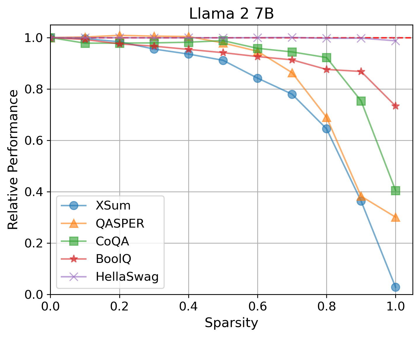
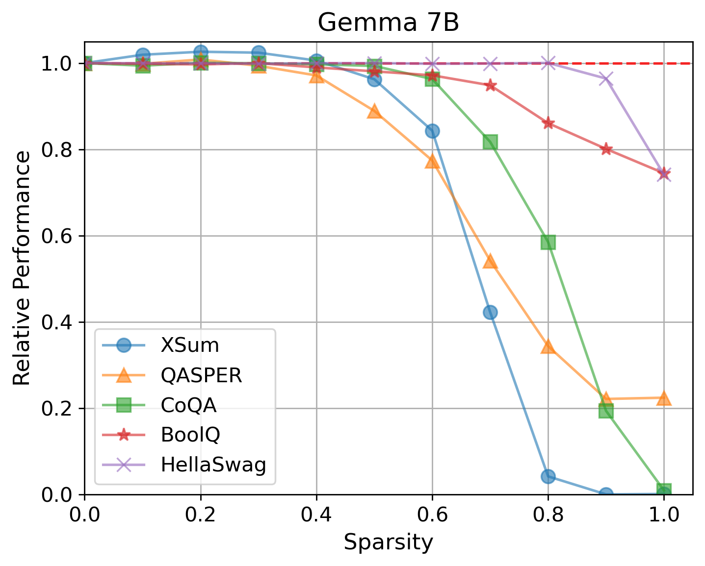
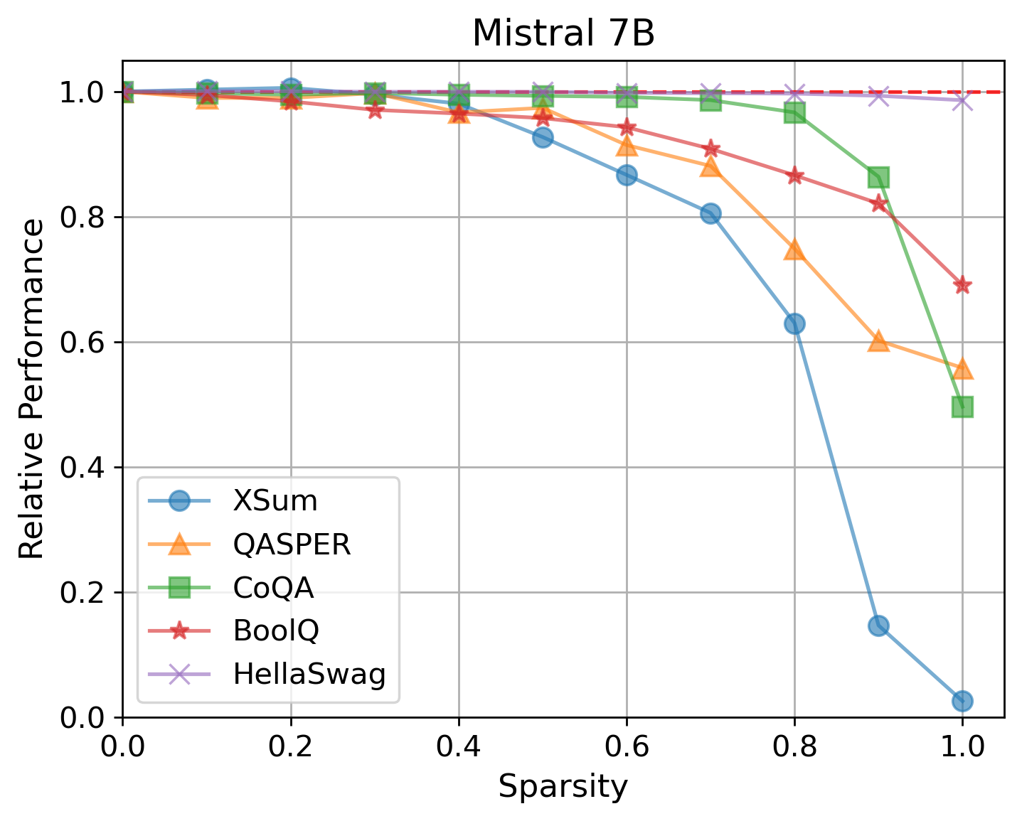
We start with a look into the relationship between the sparsity levels and performance degradation. This translates to varying when we select the top- of our statistic . To compare the performance degradation across multiple tasks, we plot the ratio of the final performance metrics between GRIFFIN and the full model in Figure 4. We see most of the performance is preserved at 50% FF sparsity in Llama 2 7B, Gemma 7B, and Mistral 7B. Different tasks have different tipping points where performance sharply drops, which may be related to the difficulty of the task [YJL+24].
| Model | XSum | CNN/DailyMail | CoQA | QASPER |
|---|---|---|---|---|
| (Rouge-1/2/L) | (Rouge-1/2/L) | (F1/EM) | (F1) | |
| Llama 2 7B | 27.15/9.06/22.62 | 10.08/0.13/9.55 | 77.35/63.88 | 26.31 |
| Magnitude | 9.71/1.31/8.59 | 9.66/0.63/9.32 | 56.59/39.93 | 12.93 |
| GRIFFIN | 24.75/7.41/20.55 | 10.97/0.66/10.37 | 77.18/63.58 | 25.76 |
| Llama 2 13B | 26.90/9.45/22.09 | 2.51/0.22/2.34 | 79.18/66.37 | 28.32 |
| Magnitude | 5.72/0.78/5.06 | 0.02/0.00/0.02 | 65.69/47.87 | 15.55 |
| GRIFFIN | 25.69/7.85/20.89 | 3.31/0.78/3.07 | 79.22/66.62 | 27.91 |
| Gemma 7B | 26.86/9.15/22.03 | 17.45/4.15/15.94 | 79.04/65.25 | 30.78 |
| Magnitude | 1.49/0.01/1.47 | 0.00/0.00/0.00 | 2.92/1.50 | 7.02 |
| GRIFFIN | 25.86/7.81/20.93 | 18.26/4.75/16.58 | 78.52/64.62 | 27.37 |
| Mistral 7B | 28.67/10.21/23.64 | 0.28/0.01/0.28 | 80.70/67.30 | 24.56 |
| Magnitude | 3.58/0.27/3.31 | 0.26/0.03/0.26 | 61.99/45.93 | 17.18 |
| GRIFFIN | 26.59/8.70/22.17 | 1.26/0.21/1.17 | 80.15/66.50 | 23.92 |
| OPT 6.7B | 23.60/7.04/19.46 | 13.85/1.54/13.04 | 68.70/54.98 | 18.53 |
| Magnitude | 1.63/0.00/1.54 | 1.20/0.00/1.17 | 31.53/16.52 | 7.28 |
| GRIFFIN | 21.17/5.42/17.58 | 13.01/1.06/12.26 | 68.99/55.00 | 17.40 |
| OPT 13B | 25.14/7.93/20.80 | 13.22/1.18/12.46 | 69.51/55.67 | 20.58 |
| Magnitude | 1.23/0.00/1.21 | 1.29/0.00/1.29 | 39.38/27.07 | 8.87 |
| GRIFFIN | 22.11/6.28/18.29 | 12.92/1.13/12.20 | 69.07/54.83 | 20.16 |
| ReluLlama 2 7B | 25.10/7.81/20.76 | 20.95/6.79/19.24 | 78.49/66.73 | 23.31 |
| Magnitude | 9.09/0.22/8.20 | 8.50/0.14/8.17 | 19.43/6.48 | 7.21 |
| GRIFFIN | 21.83/5.88/18.09 | 16.85/4.96/14.69 | 78.35/67.10 | 22.29 |
Fixing FF sparsity to be 50%, we evaluate on more tasks and models. Table 1 and Table 2 show the performance of GRIFFIN on classification and generation, respectively. We see that magnitude neuron pruning achieves reasonable results for classification but completely annihilates the original performance in most generation settings. In contrast, GRIFFIN achieves not only better performance than the baseline in most scenarios, but also preserves most of or matches the original performance on all tasks.
5.2 Efficiency
We now present efficiency metrics of GRIFFIN. We collect synthetic datasets with samples having identical lengths and average results across samples. Like many other MoE methods, GRIFFIN is ideal for single sample inputs, such as in the case of personal devices, so we use batch size 1 for these experiments. We plan to extend our method to larger batch sizes in future work. Using Hugging Face implementations of Llama 2 13B and Gemma 7B at FP16 precision, we measure the latency in different scenarios on an NVIDIA L40 GPU.
| Model | Setup | Prompt | Full | Magnitude | GRIFFIN |
|---|---|---|---|---|---|
| Llama 2 13B | 2048+128 | 0.5 | 6.8 | 5.4 / 5.0 | 5.4 / 5.1 |
| 2048+2048 | 0.5 | 119.1 | 95.0 / 83.4 | 94.9 / 82.8 | |
| Gemma 7B | 2048+128 | 0.3 | 4.5 | 4.1 / 4.2 | 4.2 / 4.1 |
| 2048+2048 | 0.3 | 78.5 | 67.7 / 65.0 | 67.4 / 65.0 |
Recalling that our magnitude selection baseline is essentially neuron pruning at generation, this has the best possible speed-up since there is no MoE overhead per sample. From Table 3, GRIFFIN matches the best case, producing up to a 1.16 and 1.25 improvement in latency for long generation at 50% FF sparsity in Gemma 7B and Llama 2 13B, respectively. This illustrates that our method is as fast as a static neuron pruned LLM during generation while being adaptive to preserve the accuracy of the full model. In offloading settings with large models, our method has the potential to further accelerate inference. For a prompt, GRIFFIN essentially performs structured pruning on the massive network, and if this pruned model can fit on a single device, it will avoid offloading for the entirety of generation.
5.3 Ablations and Analysis
Sampling-based Selection.
Here, we verify that given the statistic , top- expert selection produces better results than sampling-based methods. The methods we compare against include sampling based on the weights in and combining top- selection for half of the experts followed by weighted sampling. Based on Table 4, we can see that sampling generally degrades performance much more.
| Selection Method | XSum | CNN/DailyMail | CoQA | QASPER |
|---|---|---|---|---|
| (Rouge-1/2/L) | (Rouge-1/2/L) | (F1/EM) | (F1) | |
| Llama 2 7B | ||||
| Full | 27.15/9.06/22.62 | 10.08/0.13/9.55 | 77.35/63.88 | 26.31 |
| Top- | 24.75/7.41/20.55 | 10.97/0.66/10.37 | 77.18/63.58 | 25.76 |
| Sampling | 21.04/5.22/17.12 | 8.78/0.49/8.28 | 76.15/62.53 | 24.46 |
| Top- + Sampling | 24.35/7.08/20.07 | 10.45/0.48/9.88 | 77.12/64.17 | 25.22 |
| Gemma 7B | ||||
| Full | 26.86/9.15/22.03 | 17.45/4.15/15.94 | 79.04/65.25 | 30.78 |
| Top- | 25.86/7.81/20.93 | 18.26/4.75/16.58 | 78.52/64.62 | 27.37 |
| Sampling | 20.25/5.16/16.79 | 8.34/1.71/7.72 | 75.02/59.93 | 24.97 |
| Top- + Sampling | 24.47/7.43/19.98 | 10.93/2.60/9.98 | 76.76/62.12 | 27.09 |
Prompt vs. Generation Length.
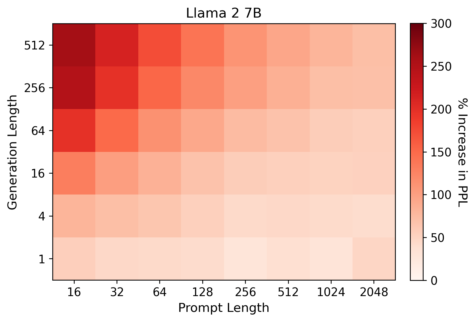
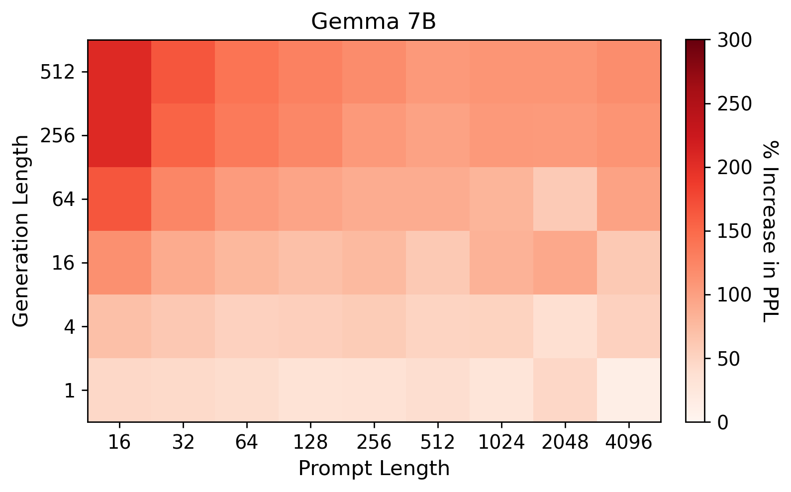
We find that GRIFFIN can potentially be made more robust for long generation by lengthening the prompt. To see this, we use language modeling on the concatenated version of WikiText to simulate generation. For a length input into the FF block, we designate the first tokens as the prompt and the last tokens as the generated portion such that . The prompt partition is used to calculate our statistic and determine the experts. The prompt partition uses the full FF block while the generation partition only uses the selected experts. When comparing the original model with GRIFFIN, we only compute the perplexity of the outputs from the generation partition since the other outputs will be identical. Based on Figure 5, GRIFFIN gets closer to the full model outputs when the prompt length increases and generation length decreases, meaning the difficulty with long generation can be suppressed with longer prompts.
Sparsity in Random Sequences.
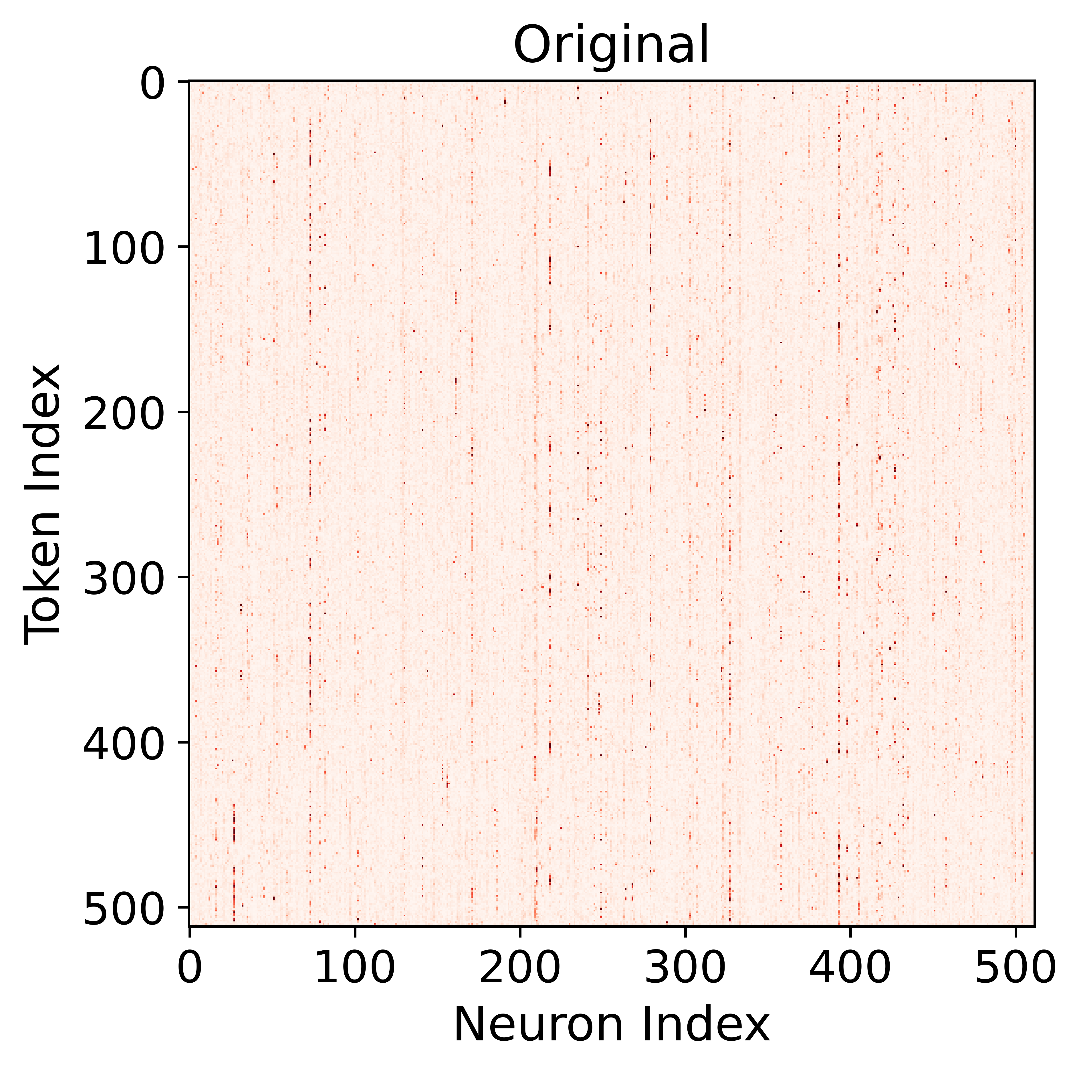
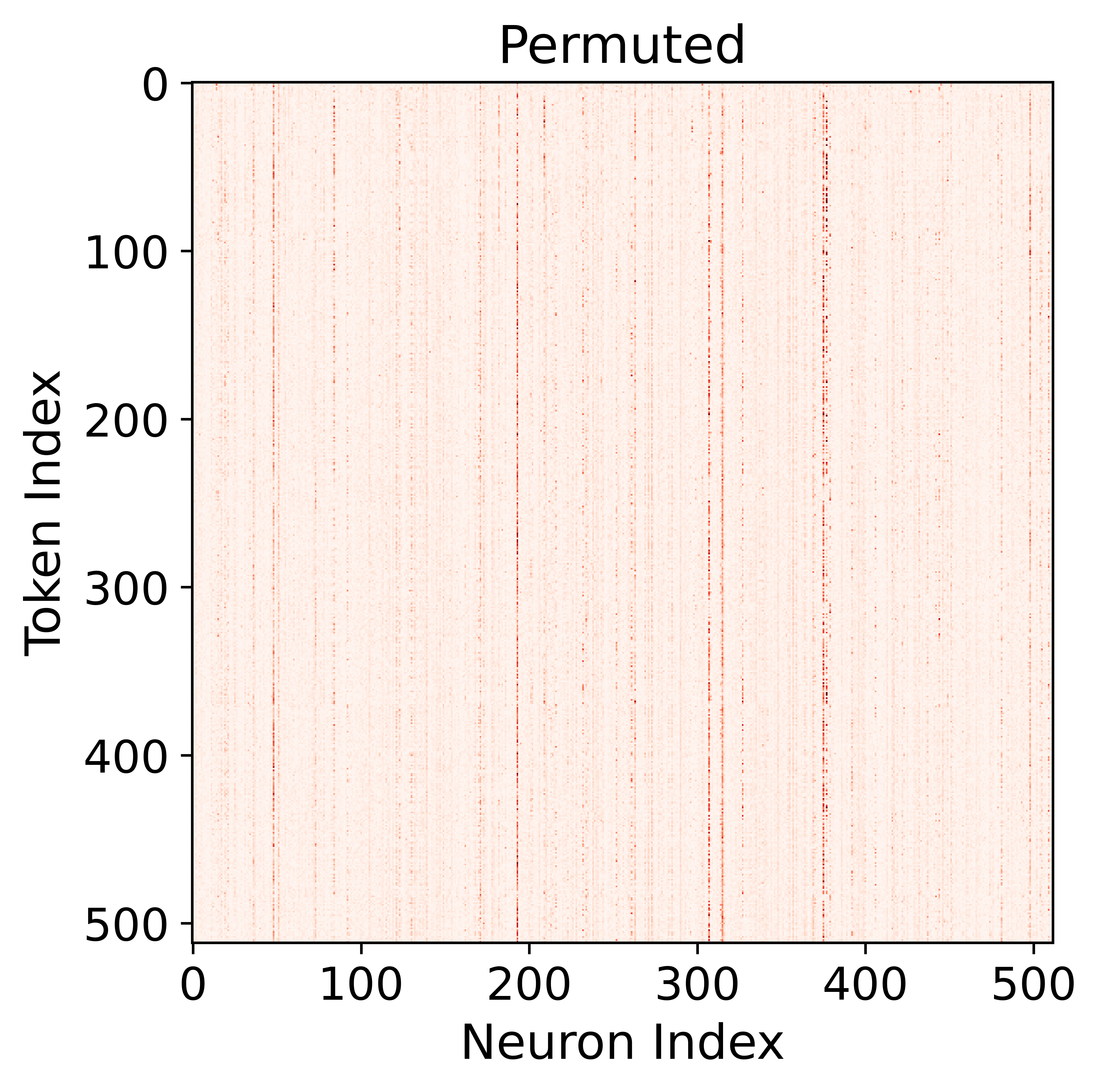
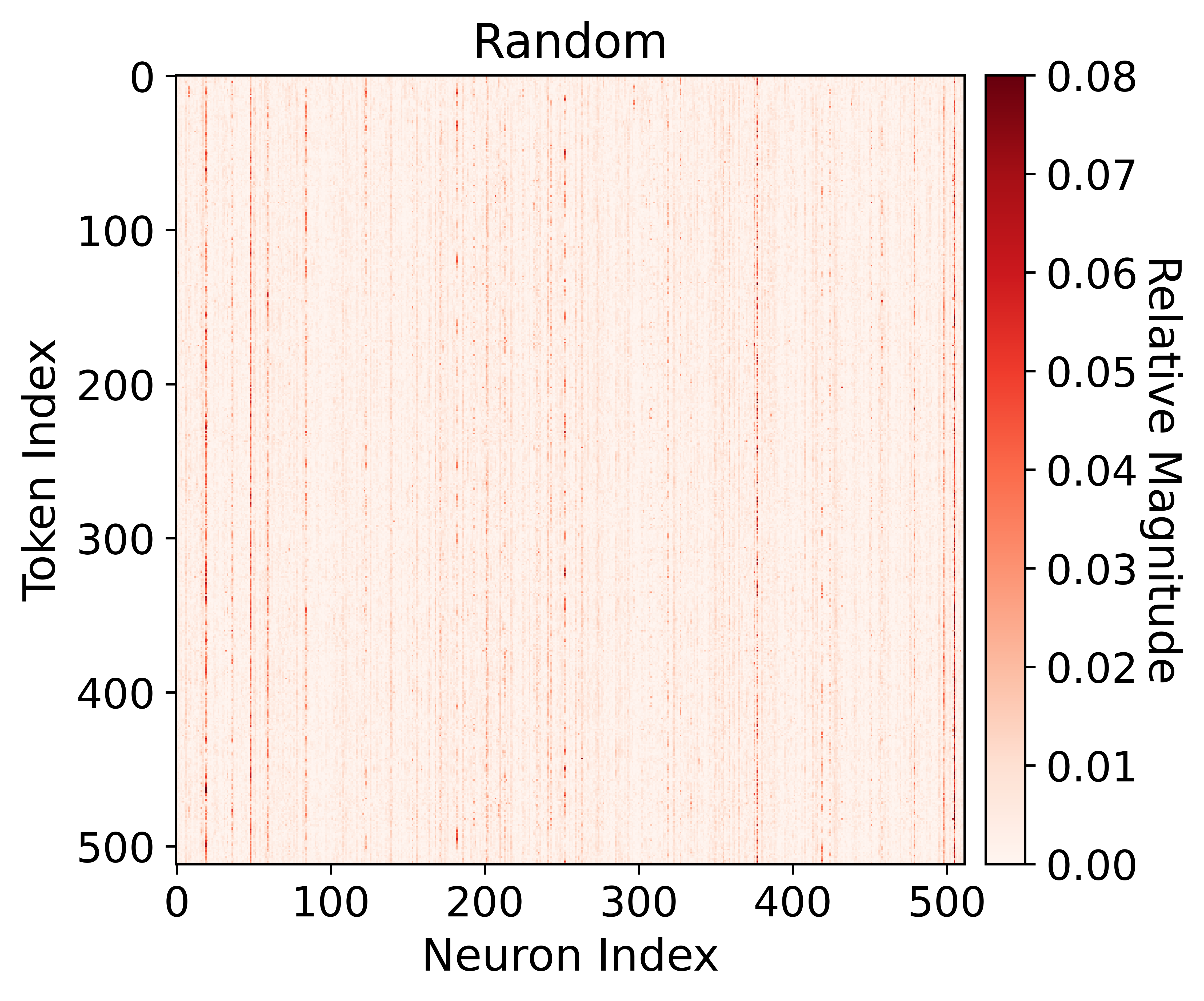
As further exploration into flocking, we investigate this phenomenon with random inputs. As input sequences, we use a sample from concatenated WikiText, a permuted version of that sample, and completely random sequence where tokens are uniformly sampled from the vocabulary. Seen in Figure 6, this structure exists in permuted and random inputs, perhaps even more consistently than in unperturbed sequences. This suggests something within language actually diversifies the activations, the cause of which would be of interest for future work.
6 Conclusion
In this work, we have shown a special form of sparsity in FF layers and a simple method to exploit it. Flocking is a curious phenomenon present in many LLMs where tokens within a sequence activate at similar intensities. This structure motivated the design of GRIFFIN, a learning-free MoE selection mechanism to remove FF neurons during inference at the sequence level which preserves the full model’s performance on a large collection of classification and generative tasks at 50% FF sparsity while achieving lower latency. Furthermore, its applicability extends beyond just ReLU-based LLMs, allowing MoE adaptation to be possible for many more models. With its straightforward algorithm and no-cost deployment, GRIFFIN expands the accessibility of numerous LLMs for generative inference.
Acknowledgements
We thank Zixin Wen for insightful discussions. The work of H. Dong is supported in part by the Wei Shen and Xuehong Zhang Presidential Fellowship at Carnegie Mellon University. The work of Y. Chi is supported in part by the grants NSF DMS-2134080 and ONR N00014-19-1-2404.
References
- [AMB+23] K. Alizadeh, I. Mirzadeh, D. Belenko, K. Khatamifard, M. Cho, C. C. Del Mundo, M. Rastegari, and M. Farajtabar. Llm in a flash: Efficient large language model inference with limited memory. arXiv preprint arXiv:2312.11514, 2023.
- [Ant24] Anthropic. The claude 3 model family: Opus, sonnet, haiku, 2024.
- [BGOFG20] D. Blalock, J. J. Gonzalez Ortiz, J. Frankle, and J. Guttag. What is the state of neural network pruning? Proceedings of machine learning and systems, 2:129–146, 2020.
- [BZB+20] Y. Bisk, R. Zellers, R. L. Bras, J. Gao, and Y. Choi. Piqa: Reasoning about physical commonsense in natural language. In Thirty-Fourth AAAI Conference on Artificial Intelligence, 2020.
- [CCE+18] P. Clark, I. Cowhey, O. Etzioni, T. Khot, A. Sabharwal, C. Schoenick, and O. Tafjord. Think you have solved question answering? try arc, the ai2 reasoning challenge. arXiv:1803.05457v1, 2018.
- [CIS23] R. Csordás, K. Irie, and J. Schmidhuber. Approximating two-layer feedforward networks for efficient transformers. arXiv preprint arXiv:2310.10837, 2023.
- [CLC+19] C. Clark, K. Lee, M.-W. Chang, T. Kwiatkowski, M. Collins, and K. Toutanova. Boolq: Exploring the surprising difficulty of natural yes/no questions. arXiv preprint arXiv:1905.10044, 2019.
- [DCC23] H. Dong, B. Chen, and Y. Chi. Towards structured sparsity in transformers for efficient inference. In Workshop on Efficient Systems for Foundation Models@ ICML2023, 2023.
- [DKK+24] L. Dery, S. Kolawole, J.-F. Kagey, V. Smith, G. Neubig, and A. Talwalkar. Everybody prune now: Structured pruning of llms with only forward passes. arXiv preprint arXiv:2402.05406, 2024.
- [DLB+21] P. Dasigi, K. Lo, I. Beltagy, A. Cohan, N. A. Smith, and M. Gardner. A dataset of information-seeking questions and answers anchored in research papers. arXiv preprint arXiv:2105.03011, 2021.
- [DLBZ22] T. Dettmers, M. Lewis, Y. Belkada, and L. Zettlemoyer. Llm. int8 (): 8-bit matrix multiplication for transformers at scale. arXiv preprint arXiv:2208.07339, 2022.
- [FA23] E. Frantar and D. Alistarh. Massive language models can be accurately pruned in one-shot. arXiv preprint arXiv:2301.00774, 2023.
- [FC18] J. Frankle and M. Carbin. The lottery ticket hypothesis: Finding sparse, trainable neural networks. arXiv preprint arXiv:1803.03635, 2018.
- [FSH04] K. Fatahalian, J. Sugerman, and P. Hanrahan. Understanding the efficiency of gpu algorithms for matrix-matrix multiplication. In Proceedings of the ACM SIGGRAPH/EUROGRAPHICS conference on Graphics hardware, pages 133–137, 2004.
- [FZS22] W. Fedus, B. Zoph, and N. Shazeer. Switch transformers: Scaling to trillion parameter models with simple and efficient sparsity. The Journal of Machine Learning Research, 23(1):5232–5270, 2022.
- [GBB+20] L. Gao, S. Biderman, S. Black, L. Golding, T. Hoppe, C. Foster, J. Phang, H. He, A. Thite, N. Nabeshima, et al. The pile: An 800gb dataset of diverse text for language modeling. arXiv preprint arXiv:2101.00027, 2020.
- [GSBL20] M. Geva, R. Schuster, J. Berant, and O. Levy. Transformer feed-forward layers are key-value memories. arXiv preprint arXiv:2012.14913, 2020.
- [GTA+23] L. Gao, J. Tow, B. Abbasi, S. Biderman, S. Black, A. DiPofi, C. Foster, L. Golding, J. Hsu, A. Le Noac’h, H. Li, K. McDonell, N. Muennighoff, C. Ociepa, J. Phang, L. Reynolds, H. Schoelkopf, A. Skowron, L. Sutawika, E. Tang, A. Thite, B. Wang, K. Wang, and A. Zou. A framework for few-shot language model evaluation, 12 2023.
- [JJNH91] R. A. Jacobs, M. I. Jordan, S. J. Nowlan, and G. E. Hinton. Adaptive mixtures of local experts. Neural computation, 3(1):79–87, 1991.
- [JLC+23] A. K. Jaiswal, S. Liu, T. Chen, Y. Ding, and Z. Wang. Instant soup: Cheap pruning ensembles in a single pass can draw lottery tickets from large models. In International Conference on Machine Learning, pages 14691–14701. PMLR, 2023.
- [JSM+23] A. Q. Jiang, A. Sablayrolles, A. Mensch, C. Bamford, D. S. Chaplot, D. d. l. Casas, F. Bressand, G. Lengyel, G. Lample, L. Saulnier, et al. Mistral 7b. arXiv preprint arXiv:2310.06825, 2023.
- [JSR+24] A. Q. Jiang, A. Sablayrolles, A. Roux, A. Mensch, B. Savary, C. Bamford, D. S. Chaplot, D. de las Casas, E. B. Hanna, F. Bressand, G. Lengyel, G. Bour, G. Lample, L. R. Lavaud, L. Saulnier, M.-A. Lachaux, P. Stock, S. Subramanian, S. Yang, S. Antoniak, T. L. Scao, T. Gervet, T. Lavril, T. Wang, T. Lacroix, and W. E. Sayed. Mixtral of experts, 2024.
- [KNH+22] S. Khan, M. Naseer, M. Hayat, S. W. Zamir, F. S. Khan, and M. Shah. Transformers in vision: A survey. ACM computing surveys (CSUR), 54(10s):1–41, 2022.
- [LDS89] Y. LeCun, J. Denker, and S. Solla. Optimal brain damage. Advances in neural information processing systems, 2, 1989.
- [LGW+21] T. Liang, J. Glossner, L. Wang, S. Shi, and X. Zhang. Pruning and quantization for deep neural network acceleration: A survey. Neurocomputing, 461:370–403, 2021.
- [LLLC21] Z. Liu, F. Li, G. Li, and J. Cheng. Ebert: Efficient bert inference with dynamic structured pruning. In Findings of the Association for Computational Linguistics: ACL-IJCNLP 2021, pages 4814–4823, 2021.
- [LWD+23] Z. Liu, J. Wang, T. Dao, T. Zhou, B. Yuan, Z. Song, A. Shrivastava, C. Zhang, Y. Tian, C. Re, et al. Deja vu: Contextual sparsity for efficient llms at inference time. In International Conference on Machine Learning, pages 22137–22176. PMLR, 2023.
- [LWLQ22] T. Lin, Y. Wang, X. Liu, and X. Qiu. A survey of transformers. AI Open, 2022.
- [LYB+22] Z. Li, C. You, S. Bhojanapalli, D. Li, A. S. Rawat, S. J. Reddi, K. Ye, F. Chern, F. Yu, R. Guo, et al. The lazy neuron phenomenon: On emergence of activation sparsity in transformers. In The Eleventh International Conference on Learning Representations, 2022.
- [LYZ+23] Y. Li, Y. Yu, Q. Zhang, C. Liang, P. He, W. Chen, and T. Zhao. Losparse: Structured compression of large language models based on low-rank and sparse approximation. arXiv preprint arXiv:2306.11222, 2023.
- [LZH+24] B. Liu, Z. Zhang, P. He, Z. Wang, Y. Xiao, R. Ye, Y. Zhou, W.-S. Ku, and B. Hui. A survey of lottery ticket hypothesis. arXiv preprint arXiv:2403.04861, 2024.
- [MAM+23] I. Mirzadeh, K. Alizadeh, S. Mehta, C. C. Del Mundo, O. Tuzel, G. Samei, M. Rastegari, and M. Farajtabar. Relu strikes back: Exploiting activation sparsity in large language models. arXiv preprint arXiv:2310.04564, 2023.
- [MFW23] X. Ma, G. Fang, and X. Wang. Llm-pruner: On the structural pruning of large language models. Advances in neural information processing systems, 36:21702–21720, 2023.
- [MXBS16] S. Merity, C. Xiong, J. Bradbury, and R. Socher. Pointer sentinel mixture models, 2016.
- [NBZ+23] S. Nerella, S. Bandyopadhyay, J. Zhang, M. Contreras, S. Siegel, A. Bumin, B. Silva, J. Sena, B. Shickel, A. Bihorac, et al. Transformers in healthcare: A survey. arXiv preprint arXiv:2307.00067, 2023.
- [NCL18] S. Narayan, S. B. Cohen, and M. Lapata. Don’t give me the details, just the summary! topic-aware convolutional neural networks for extreme summarization. arXiv preprint arXiv:1808.08745, 2018.
- [NZG+16] R. Nallapati, B. Zhou, C. Gulcehre, B. Xiang, et al. Abstractive text summarization using sequence-to-sequence rnns and beyond. arXiv preprint arXiv:1602.06023, 2016.
- [PSBW23] M. Piórczyński, F. Szatkowski, K. Bałazy, and B. Wójcik. Exploiting transformer activation sparsity with dynamic inference. arXiv preprint arXiv:2310.04361, 2023.
- [RBG11] M. Roemmele, C. A. Bejan, and A. S. Gordon. Choice of plausible alternatives: An evaluation of commonsense causal reasoning. In 2011 AAAI Spring Symposium Series, 2011.
- [RCM19] S. Reddy, D. Chen, and C. D. Manning. Coqa: A conversational question answering challenge. Transactions of the Association for Computational Linguistics, 7:249–266, 2019.
- [RPJ+19] J. W. Rae, A. Potapenko, S. M. Jayakumar, C. Hillier, and T. P. Lillicrap. Compressive transformers for long-range sequence modelling. arXiv preprint, 2019.
- [Sha20] N. Shazeer. Glu variants improve transformer. arXiv preprint arXiv:2002.05202, 2020.
- [SLBK23] M. Sun, Z. Liu, A. Bair, and J. Z. Kolter. A simple and effective pruning approach for large language models. arXiv preprint arXiv:2306.11695, 2023.
- [SSI+22] U. Shaham, E. Segal, M. Ivgi, A. Efrat, O. Yoran, A. Haviv, A. Gupta, W. Xiong, M. Geva, J. Berant, et al. Scrolls: Standardized comparison over long language sequences. arXiv preprint arXiv:2201.03533, 2022.
- [SWSL23] M. Santacroce, Z. Wen, Y. Shen, and Y. Li. What matters in the structured pruning of generative language models? arXiv preprint arXiv:2302.03773, 2023.
- [TAB+23] G. Team, R. Anil, S. Borgeaud, Y. Wu, J.-B. Alayrac, J. Yu, R. Soricut, J. Schalkwyk, A. M. Dai, A. Hauth, et al. Gemini: a family of highly capable multimodal models. arXiv preprint arXiv:2312.11805, 2023.
- [Tea23] S. Team. Sparse large language models with relu activation, 2023.
- [TMH+24] G. Team, T. Mesnard, C. Hardin, R. Dadashi, S. Bhupatiraju, S. Pathak, L. Sifre, M. Rivière, M. S. Kale, J. Love, et al. Gemma: Open models based on gemini research and technology. arXiv preprint arXiv:2403.08295, 2024.
- [TMS+23] H. Touvron, L. Martin, K. Stone, P. Albert, A. Almahairi, Y. Babaei, N. Bashlykov, S. Batra, P. Bhargava, S. Bhosale, et al. Llama 2: Open foundation and fine-tuned chat models. arXiv preprint arXiv:2307.09288, 2023.
- [VSP+17] A. Vaswani, N. Shazeer, N. Parmar, J. Uszkoreit, L. Jones, A. N. Gomez, Ł. Kaiser, and I. Polosukhin. Attention is all you need. Advances in neural information processing systems, 30, 2017.
- [WWB19] Y. E. Wang, G.-Y. Wei, and D. Brooks. Benchmarking tpu, gpu, and cpu platforms for deep learning. arXiv preprint arXiv:1907.10701, 2019.
- [XGZC23] M. Xia, T. Gao, Z. Zeng, and D. Chen. Sheared llama: Accelerating language model pre-training via structured pruning. arXiv preprint arXiv:2310.06694, 2023.
- [XZC22] M. Xia, Z. Zhong, and D. Chen. Structured pruning learns compact and accurate models. arXiv preprint arXiv:2204.00408, 2022.
- [YJL+24] L. Yin, A. Jaiswal, S. Liu, S. Kundu, and Z. Wang. Pruning small pre-trained weights irreversibly and monotonically impairs "difficult" downstream tasks in llms, 2024.
- [YYB+24] V. Yerram, C. You, S. Bhojanapalli, S. Kumar, P. Jain, P. Netrapalli, et al. Hire: High recall approximate top- estimation for efficient llm inference. arXiv preprint arXiv:2402.09360, 2024.
- [ZBC+24] H. Zheng, X. Bai, B. Chen, F. Lai, and A. Prakash. Learn to be efficient: Build structured sparsity in large language models. arXiv preprint arXiv:2402.06126, 2024.
- [ZHB+19] R. Zellers, A. Holtzman, Y. Bisk, A. Farhadi, and Y. Choi. Hellaswag: Can a machine really finish your sentence? arXiv preprint arXiv:1905.07830, 2019.
- [ZLL+21] Z. Zhang, Y. Lin, Z. Liu, P. Li, M. Sun, and J. Zhou. Moefication: Transformer feed-forward layers are mixtures of experts. arXiv preprint arXiv:2110.01786, 2021.
- [ZRG+22] S. Zhang, S. Roller, N. Goyal, M. Artetxe, M. Chen, S. Chen, C. Dewan, M. Diab, X. Li, X. V. Lin, T. Mihaylov, M. Ott, S. Shleifer, K. Shuster, D. Simig, P. S. Koura, A. Sridhar, T. Wang, and L. Zettlemoyer. Opt: Open pre-trained transformer language models, 2022.
Appendix A Gating Metric
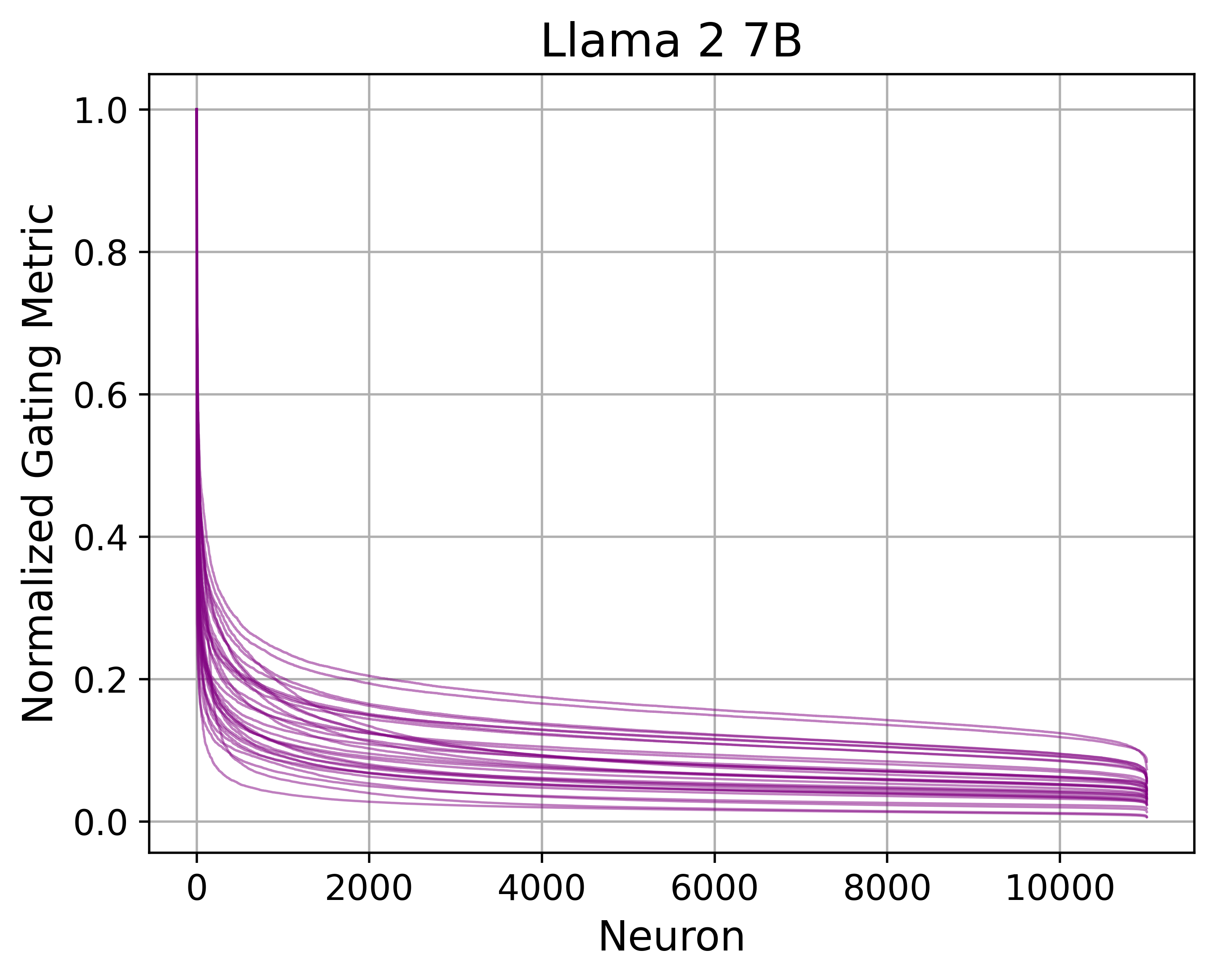
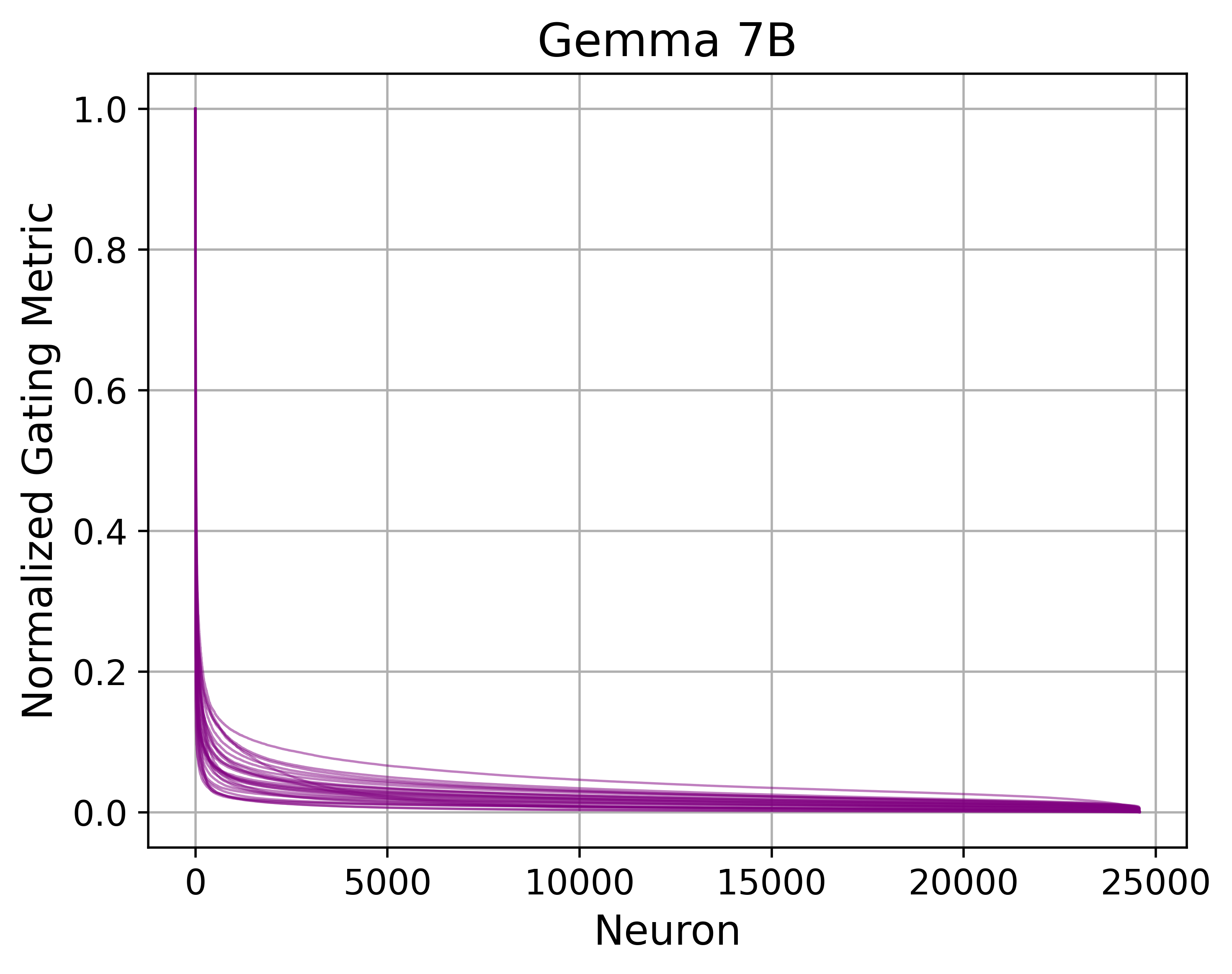
Here we present visualizations of our gating statistic from (6). For a single sample, we find and sort the entries normalized between 0 and 1 in Figure 7. In both models, values in are heavily concentrated in a handful of features. Since aggregates the relative activation magnitudes across tokens, this implies can capture heavily and frequently activated neurons.
Appendix B More Flocking Examples
We provide more example of flocking across different layers of the LLM. Figure 8 and Figure 9 show flocking in Gemma 7B. Figure 10 and Figure 11 show flocking in Llama2 7B. Flocking in Gemma 7B is more visually distinct while activations in Llama2 7B are more distributed.


