figure \cftpagenumbersofftable
Harnessing Data and Physics for Deep Learning Phase Recovery
Abstract
Phase recovery, calculating the phase of a light wave from its intensity measurements, is essential for various applications, such as coherent diffraction imaging, adaptive optics, and biomedical imaging. It enables the reconstruction of an object’s refractive index distribution or topography as well as the correction of imaging system aberrations. In recent years, deep learning has been proven to be highly effective in addressing phase recovery problems. Two main deep learning phase recovery strategies are data-driven (DD) with supervised learning mode and physics-driven (PD) with self-supervised learning mode. DD and PD achieve the same goal in different ways and lack the necessary study to reveal similarities and differences. Therefore, in this paper, we comprehensively compare these two deep learning phase recovery strategies in terms of time consumption, accuracy, generalization ability, ill-posedness adaptability, and prior capacity. What’s more, we propose a co-driven (CD) strategy of combining datasets and physics for the balance of high- and low-frequency information. The codes for DD, PD, and CD are publicly available at https://github.com/kqwang/DLPR.
keywords:
phase recovery, deep learning, computational imaging*Kaiqiang Wang, \linkablekqwang.optics@gmail.com; Edmund Y. Lam, \linkableelam@eee.hku.hk
1 Introduction
Phase recovery refers to a class of methods that recover the phase of light waves from intensity measurements [1]. It is active in various fields of imaging and detection, such as in bioimaging for obtaining the refractive index or thickness distribution of tissues or cells [2], in adaptive optics for characterizing aberrant wavefront [3], in coherent diffraction imaging for detecting structural information of nanomolecules [4], and in material inspection for measuring surface profile [5].
Since optical detectors, such as charge-coupled device sensors, can only record the intensity/amplitude but lose the phase, one has to recover the phase from the recorded intensity indirectly. And precisely because of the loss of the phase, it is ill-posed to directly calculate the phase on the object plane from the only amplitude on the measurement plane through the forward physical model. On the one hand, the phase can be iteratively retrieved from intensity measurements with prior knowledge, i.e., phase retrieval [6]. On the other hand, by incorporating additional information, this problem can be transformed into a well-posed one and solved directly, such as holography or interferometry with reference light [7, 8], Shack-Hartmann wavefront sensing with micro-lens array [9, 10], and the transport of intensity equation with multiple through-focus amplitudes [11, 12].
In recent years, deep learning, with artificial neural networks as the carrier, has brought new solutions to phase recovery, where the core idea is to train neural networks to learn the mapping relationship from intensity measurements to the light wave phase [13, 1]. As illustrated in Fig. 1, the training of neural networks can be driven either supervised by paired datasets as an implicit prior (data-driven, DD) or self-supervised by physical models as an explicit prior (physics-driven, PD) [1].
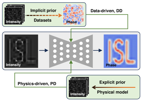
Sinha et al. [14] first demonstrated DD phase recovery with paired diffraction-phase datasets, obtained by recording diffraction images of virtual phase objects loaded on a spatial light modulator. Subsequently, DD phase recovery was successively extended to in-line holography [15], coherent diffraction imaging [16], Fourier ptychography [17], off-axis holography [18], Shack-Hartmann wavefront sensing [19], transport of intensity equation [20], optical diffraction tomography [21], and electron diffractive imaging [22]. In addition, several studies focused on more efficient neural network structures for phase recovery, such as Bayesian neural network [23], generative adversarial network [24], Y-Net [25, 26], residual capsule network [27], recurrent neural network [28], Fourier imager network [29, 30], and neural architecture search [31]. Some studies also used data-driven methods for pre- or post-processing of phase recovery, such as defocus distance prediction [32], resolution enhancement [33], phase unwrapping [34], and classification [35, 36].
The idea of PD phase recovery was first introduced by Boominathan et al. [37] in their simulation work on Fourier ptychography. Wang et al. [38] first experimentally used PD to iteratively infer the phase of a phase-only object from its diffraction image directly on an untrained/initialized neural network. Afterward, it was subsequently extended to the cases of unknown defocus distances [39], dual wavelengths [40], and complex-valued amplitude objects [41, 42]. In the quest for faster inference times, PD and a large number of intensity measurements were used for neural network pre-training [41, 42, 43, 44, 45]. Further, refinement of pre-trained neural networks by PD achieved higher accuracy with lower inference time [46, 47].
DD and PD achieve the same goal in different ways and are being studied in different contexts to achieve efficient phase recovery. Therefore, it is necessary and meaningful to compare them under the same context. In this paper, we introduce the principles of DD and PD, and comparatively study them in terms of time consumption, accuracy, generalization ability, ill-posedness adaptability, and prior capacity. We also combine DD and PD as a co-driven (CD) strategy to train neural networks for high- and low-frequency information balance. What’s more, to facilitate readers to get started with deep learning phase recovery quickly, we release the demonstrations of DD, PD, and CD at https://github.com/kqwang/DLPR.
2 Principles
Here, we consider a classic phase recovery paradigm, recovering the phase or complex-valued amplitude of a light wave from its in-line hologram (diffraction pattern). For an object illuminated by a coherent plane wave, its hologram can be written as
| (1) |
where is the hologram, is the amplitude of light wave, is the phase of light wave, and is the forward propagation function, respectively. For a phase object, we assume . Then, the purpose of phase recovery is to formulate the inverse mapping of :
| (2) |
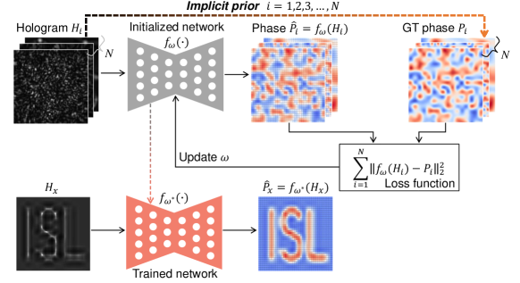
With a supervised learning mode, DD trains neural networks with paired hologram-phase datasets as an implicit prior to learn this inverse mapping [14]:
| (3) |
where denotes the square of the -norm (or other distance functions) and is a neural network with trainable parameters , like weights and biases. When the optimization is complete, the trained neural network is used as an inverse mapper to infer the corresponding phase from its hologram of an unseen object that is not in training dataset:
| (4) |
A visual representation of DD can be seen in Fig. 2, in which holograms and phases are used as the input and ground truth (GT) of the neural network, respectively. The training dataset, collected through experiments or numerical simulations, typically contains paired data from thousands to hundreds of thousands. The training stage usually lasts for hours or even days but only takes one time. After that, the trained neural network quickly infers the phase of the unseen object after being fed its hologram.
For physical processes that can be well modeled, such as phase recovery, PD is another available strategy. With a self-supervised learning mode, PD uses a numerical propagation as an explicit prior to drive the training or inference of neural networks (Fig. 3). Different from DD, which calculates the loss function in the phase domain, PD converts the network output from the phase domain to the hologram domain via numerical propagation and then calculates the loss function. This explicit prior can be utilized in three ways: untrained PD (uPD) [38], trained PD (tPD) [44], and tPD with refinement (tPDr) [46].
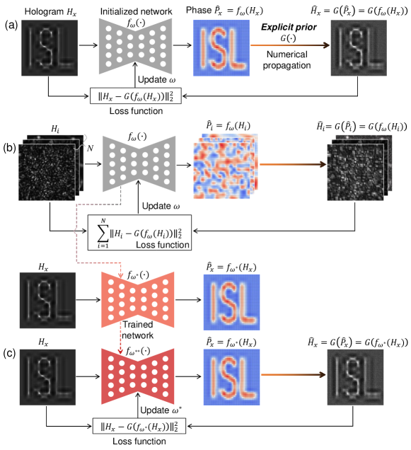
With driving of the explicit prior , uPD iteratively optimizes an untrained neural network to infer the phase of an unseen object from its hologram (Fig. 3a):
| (5) | ||||
In tPD, the explicit prior is employed to train an untrained neural network with intensity-only training dataset as input, and then the trained neural network infers the phase of an unseen object from its hologram (Fig. 3b):
| (6) | ||||
In tPDr, the trained neural network of tPD is iteratively fine-tuned on the hologram of the unseen object (Fig. 3c):
| (7) | ||||
For the sake of clarity, we summarize DD, uPD, tPD, and tPDr according to their requirements for the physical model, the training dataset, the number of cycles needed for inference, and the learning mode in Table 1.
| Strategy | Physics requirement | Dataset requirement | Inference cycles | Learning mode |
|---|---|---|---|---|
| DD | No | Hologram-phase dataset | One time | Supervised |
| uPD | Numerical propagation | No | Multi times | self-supervised |
| tPD | Numerical propagation | Hologram-only dataset | One time | self-supervised |
| tPDr | Numerical propagation | Hologram-only dataset | Multi times | self-supervised |
3 Comparisons
To avoid unnecessary distraction factors, all datasets used for comparison are generated through numerical simulation based on ImageNet, LFW, and MNIST, see Appendix A. All methods use the same U-Net-based neural network, the specific structure of which is described in the Supplementary Material of Ref. 48. The implementation of the neural network is set uniformly, see Appendix B. The average peak signal-to-noise ratio (PSNR) and structural similarity index measure (SSIM) are used to quantify the inference accuracy.
3.1 Comparison of time consumption and accuracy
In this section, ImageNet is used for dataset generation. We summarize the training settings and inference evaluation of DD, uPD, tPD, and tPDr in Table 2.
| Strategy | training datasets | Inference cycles | Inference time | PSNR | SSIM |
| DD | 10,000 pairs | 1 | 0.02 seconds | 19.9 | 0.68 |
| uPD | 0 | 10,000 | 800 seconds | 25.6 | 0.94 |
| tPD | 10,000 pairs | 1 | 0.02 seconds | 18.5 | 0.69 |
| tPDr | 10,000 inputs | 1,000 | 80 seconds | 25.1 | 0.93 |
In terms of time consumption, DD, tPD, and tPDr all require pre-training before inference, thus consuming hours or even more for neural network optimization, whereas uPD performs inference for the tested sample directly on an untrained neural network. During the inference stage of DD and tPD, the hologram of the tested sample passes through the trained neural network once in one second, while the inference process for uPD and tPDr takes several minutes for iteration.
As for the inference accuracy, the PSNR and SSIM of DD and tPD which do quick inference once after pre-training are basically the same, and both significantly lower than uPD and tPDr which do inference multiple times. Due to the prior knowledge introduced in the pre-training stage, the initial inference of tPDr is closer to the target solution, which makes it get the same accuracy with shorter inference cycles than uPD. Specifically, with comparable accuracy, the inference time of tPDr is one-tenth that of uPD.
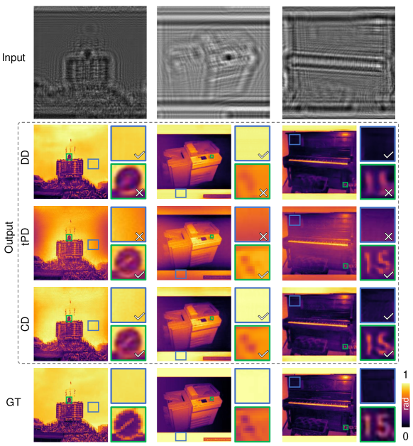
Although having the same accuracy index (Table 2), the inference result of tPD shows better high-frequency detailed information while that of DD shows better low-frequency background information (Figure 4). According to the frequency principle, deep neural networks are more inclined to learn low-frequency information in the data [49]. DD learns the hologram-phase mapping relationship through the loss function in the phase domain, while PD uses numerical propagation to transfer it from the phase domain to the hologram domain. On the one hand, as shown in the white curve on the left side of Figure 4, the high-frequency phase information (steeper curve) is recorded in the diffraction fringes of the hologram which contains a more balanced high- and low-frequency information (smoother curve). This is more favorable for PD to learn those high-frequency phase information from the loss function in the hologram domain. On the other hand, the low-frequency phase causes only little contrast in the hologram, making it difficult for PD to learn low-frequency phase information, especially the plane background phase.
In order to balance the high- and low-frequency phase information learned by the neural network, we propose to use both dataset and physics for the neural network training, named CD. The loss function of CD is derived from the weighted sum of the data-driven term and physical-driven term:
| (8) |
where is the weight used to control the contribution of the data-driven term and physical-driven term, which is set to 0.3. As illustrated in Figure 5, compared to the low-frequency-tendency DD and high-frequency-tendency tPD, CD takes into account both the high-frequency phase (see the blue box) and low-frequency phase (see the green box).
3.2 Comparison of generalization abilit
To compare the generalization ability of DD and tPD, ImageNet, LFW, and MNIST are used to generate datasets for neural network training and cross-inference, respectively. ImageNet represents dense samples, MNIST represents sparse samples, and LFW is somewhere in between. In Fig. 6, we show the cross-inference results and their absolute error maps of a sample from ImageNet, LFW, and MNIST, and attach the average SSIM on the testing dataset below each result.
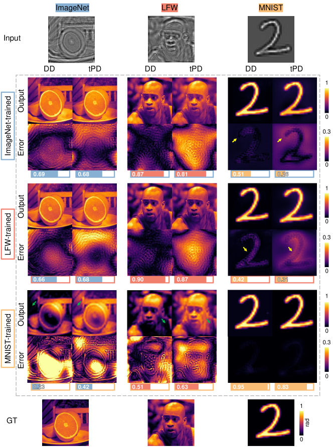
Overall, the dataset is the main factor affecting the generalization ability of the trained neural network. Specifically, the neural networks trained by ImageNet and LFW generally perform better on all three testing datasets, while the neural networks trained by MNIST can only infer the overall distribution of ImageNet and LFW but lack detailed information. Admittedly, MNIST itself lacks detailed information, so it is reasonable that neural networks trained with it would not be able to fully infer detailed information about ImangeNet and LFW. In this extreme case, tPD is significantly better than DD, both in terms of inference results and SSIM. As can be seen in Fig. 6, tPD infers more detailed information than DD (marked by the green arrow). Another thing worth noting is that for the case of using neural networks trained by ImageNet and LFW to infer MNIST, although the inference results of both tPD and DD appear to be ideal, the SSIM of tPD is much lower than that of DD. As can be seen from the absolute error maps (marked by the yellow arrow), the error in the background part of tPD is relatively larger than that of DD, which confirms a conclusion in Sec. 3.1 that tPD is not good at low-frequency phase information, especially the plane background phase.
3.3 Comparison of ill-posedness adaptability
Let us consider a more ill-posed case of using a neural network to simultaneously infer phase and amplitude from a hologram. In dataset generation, ImageNet, LFW, and MNIST are used to get samples containing phase and amplitude respectively, and the corresponding holograms are calculated through numerical propagation. Given that the neural network needs to output both phase and amplitude, we modified the original U-Net by paralleling another up-sampling path to build a Y-Net [25]. The way tPD trains the neural network has not changed, except that there is an amplitude term in the loss function:
| (9) | ||||
where denotes the Y-Net that outputs phase and amplitude simultaneously. The loss function of DD is derived by weighted summation of the phase term and amplitude term:
| (10) | ||||
where and denote the phase path and amplitude path of Y-Net, respectively, is the weight used to control the contribution of the phase term and amplitude term, which is set to 0.1.
The inference results of DD and tPD with single hologram input are shown in the blue part of Fig. 7. DD can infer the phase and amplitude at the same time, because the implicit mapping relationship from holograms to phase and amplitude is completely included in the paired dataset used for the network training. As for tPD, obvious artifacts appear in the inference results and its SSIM is reduced accordingly. This means that although there are many undesirable components in the inference result, the hologram corresponding to this non-ideal phase and amplitude matches the hologram of the sample. That is, the situation of using a hologram to infer both phase and amplitude simultaneously is severely ill-posed for tPD.
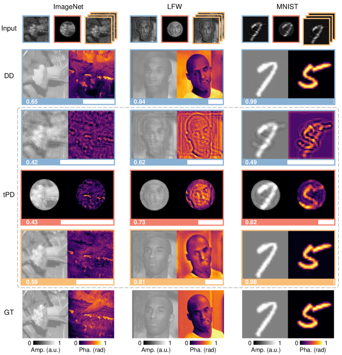
Here we show two solutions for this ill-posedness of tPD. For one thing, we introduce an aperture constraint in the sample plane to reduce the difficulty of tPD phase recovery [41]:
| (11) | ||||
where is the aperture constraint with radius which is set to 80 pixels, and denotes the zero matrix of size where is set to 256. After introducing aperture constraints, the inference results of tPD for the three datasets are improved to varying degrees (see the red part of Fig. 7). MNIST has the largest improvement, followed by LFW, and ImageNet has such limited improvement. This means that the aperture constraint works well for simple cases with less information but can hardly deal with more difficult samples. For another thing to further reduce the ill-posedness of tPD, we introduce more prior knowledge by using multiple holograms with different defocus distances as network inputs [44]. In this case, the loss function contains three terms corresponding to different defocus distances:
| (12) |
where donate the numerical propagation of different distances, and donate holograms with different defocus distances, where are set to 20mm, 40mm, and 60mm respectively. Compared to a single hologram input, two more holograms introduce sufficient prior knowledge for tPD, resulting in a significant improvement in the trained neural network, both for the simple MNIST and the complex LFW and ImageNet (see the yellow part of Fig. 7).
3.4 Comparison of prior capacity
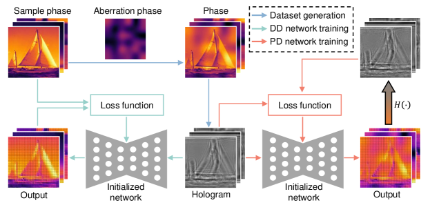
tPD uses numerical propagation as an explicit prior to train the neural network, so the neural network learns priors from numerical propagation. DD trains a neural network with paired datasets, which means that the neural network learns all implicit priors contained in the dataset even if it is outside the numerical propagation. For example, in the presence of imaging aberration, there will be both sample and aberration information in the hologram. Here, we use ImageNet as the sample phase and a random phase generated by the random matrix enlargement (RME) [34, 48] as the aberration phase to generate a dataset for the comparison of DD and tPD. The process of dataset generation and network training is shown in Fig. 8, where blue represents the dataset generation part, green represents the network training part of DD, and red represents the network training part of tPD.
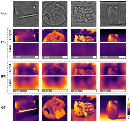
We illuminate the inference results and absolute error maps of four samples in Figure 9. As expected, DD infers the sample phase while removing the imaging aberration phase, while the inference result of tPD includes both the sample phase and the aberration phase. Accordingly, the SSIM of DD is much higher than that of tPD. In DD, the hologram contains unwanted aberration information, but the ground truth only contains sample information, which means that the dataset implicitly contains both the prior for phase recovery and the prior for aberration removal. As for tPD, the prior for the network training is derived from numerical propagation, which allows both the sample information and the aberration information in the hologram to be recovered. It should be noted that the results of uPD also contain the unwanted aberration phase just like that of tPD.
4 Experimental tests
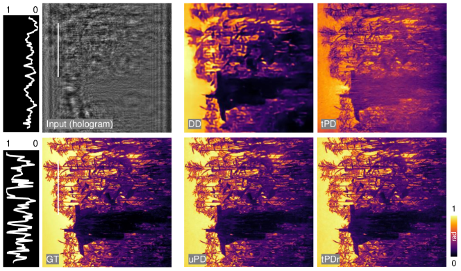
We compare DD, tPD, CD, and uPD(tPDr) using experimental holograms of standard phase objects. This experimental hologram with a defocus distance of 8.78mm is from an open-source dataset of Ref 50. To match the defocus distance of the experimental hologram, we use ImageNet to generate corresponding datasets for the network training. Inference results for all methods are given in Fig. 10.
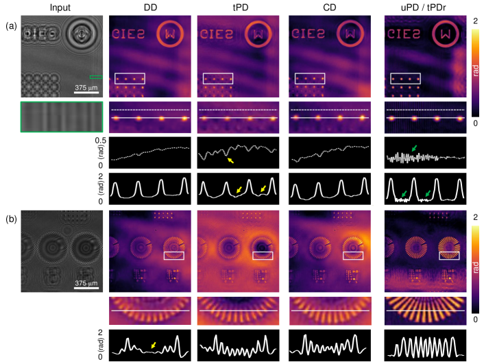
Overall, uPD and tPDr with multiple-times inferences have the best results, as seen from the neatly drawn peaks and valleys. It should be noted that due to the presence of redundant diffraction fringes at the edge of the hologram (see the green box in Fig. 10(a)), unwanted fluctuations appear in the background of the uPD and tPDr inference results (see the green arrows in Fig. 10(a)). Among the remaining one-time inference methods, the background fluctuations of the tPD results are larger (see the yellow arrows in Fig. 10(a)), while the detailed information of the DD results is weaker (see the yellow arrows in Fig. 10(b)). As a combination of DD and tPD, CD better considers detailed and background information. It should be noted that as the training dataset further expands, the neural network’s accuracy will increase accordingly.
5 Conclusion
We introduced the principles of DD and PD strategies for deep learning phase recovery in the same context. On this basis, we compared the time consumption and accuracy of DD, uPD, tPD, and tPDr, and found that uPD and tPDr achieve the highest accuracy with multiple inferences, tPD prefers the high-frequency detailed phase while DD favors the low-frequency background phase. Therefore, we proposed CD to balance high- and low-frequency information. Furthermore, we found that tPD generalizes better than DD for the case of inferring dense samples using neural networks trained on sparse samples. As for the case of inferring phase and amplitude simultaneously, we revealed the reason why DD is stronger than tPD, that is, the dataset for DD implicitly contains the mapping relationship from holograms to phase and amplitude while tPD may encounter situations where multiple network outputs phases and amplitudes correspond to a same hologram. To alleviate the ill-posedness of tPD, we proposed solutions by aperture constraints or multiple hologram inputs. In addition, we used the case of imaging aberration to demonstrate that DD can learn more about the prior implicit in the dataset whereas PD can only learn the prior in numerical propagation. Finally, we verified with experimental data that uPD and tPDr have the highest accuracy and that CD balances high- and low-frequency information better than DD and tPD.
Appendix A Dataset generation
Three publicly available image datasets (ImageNet, LFW, and MNIST) are used to generate phases and amplitudes, and then the corresponding holograms at a certain propagation distance are computed via numerical propagation. The training and testing datasets contain 10,000 and 100 data, respectively. The size of all data is set to . The propagation distance is set to 20 mm and 8.78 mm for the simulation comparisons and the experimental tests, respectively.
Appendix B Network implementation
The Adam optimizer with an initial learning rate of 0.001 is adopted to update the weights and biases. The neural network training epoch of DD and PD is set to 100. The inference cycles of uPD and tPDr are set to 10,000 and 1000, respectively. All the neural networks are based on Pytorch (2.0.0) with Python (3.8.18). All operators run on a compute server equipped with AMD Ryzen Threadripper PRO 3955WX and NVIDIA GeForce RTX 3090.
Disclosures
The authors declare no competing interests.
Acknowledgments
The work was supported in part by the Research Grants Council of Hong Kong (GRF 17201620, GRF 17200321, RIF R7003-21).
References
- [1] K. Wang, L. Song, C. Wang, et al., “On the use of deep learning for phase recovery,” Light: Science & Applications 13(1), 4 (2024). [doi:10.1038/s41377-023-01340-x].
- [2] Y. Park, C. Depeursinge, and G. Popescu, “Quantitative phase imaging in biomedicine,” Nature Photonics 12(10), 578–589 (2018). [doi:10.1038/s41566-018-0253-x].
- [3] R. K. Tyson and B. W. Frazier, Principles of Adaptive Optics, CRC Press, Boca Raton, 5th edn. ed. (2022).
- [4] J. Miao, P. Charalambous, J. Kirz, et al., “Extending the methodology of X-ray crystallography to allow imaging of micrometre-sized non-crystalline specimens,” Nature 400(6742), 342–344 (1999). [doi:10.1038/22498].
- [5] R. Leach, Ed., Optical Measurement of Surface Topography, Springer, Berlin, Heidelberg (2011).
- [6] M. V. Klibanov, P. E. Sacks, and A. V. Tikhonravov, “The phase retrieval problem,” Inverse Problems 11(1), 1–28 (1995). [doi:10.1088/0266-5611/11/1/001].
- [7] D. Gabor, “A New Microscopic Principle,” Nature 161, 777–778 (1948). [doi:10.1038/161777a0].
- [8] J. W. Goodman, Introduction to Fourier Optics, W.H. Freeman, New York, 4th edn. ed. (2017).
- [9] J. Hartmann, “Bermerkungen über den bau und die justierung von spektrographen,” Zeitschrift für Instrumentenkunde 20, 47–58 (1900).
- [10] R. V. Shack and B. C. Platt, “Production and use of a lenticular Hartmann screen,” Journal of the Optical Society of America 61, 656–661 (1971).
- [11] M. R. Teague, “Deterministic phase retrieval: A Green’s function solution,” Journal of the Optical Society of America 73(11), 1434–1441 (1983). [doi:10.1364/JOSA.73.001434].
- [12] C. Zuo, J. Li, J. Sun, et al., “Transport of intensity equation: A tutorial,” Optics and Lasers in Engineering 135, 106187 (2020). [doi:10.1016/j.optlaseng.2020.106187].
- [13] G. Barbastathis, A. Ozcan, and G. Situ, “On the use of deep learning for computational imaging,” Optica 6(8), 921–943 (2019). [doi:10.1364/OPTICA.6.000921].
- [14] A. Sinha, J. Lee, S. Li, et al., “Lensless computational imaging through deep learning,” Optica 4(9), 1117–1125 (2017). [doi:10.1364/OPTICA.4.001117].
- [15] H. Wang, M. Lyu, and G. H. Situ, “eHoloNet: A learning-based end-to-end approach for in-line digital holographic reconstruction,” Optics Express 26(18), 22603–22614 (2018). [doi:10.1364/OE.26.022603].
- [16] M. J. Cherukara, Y. S. G. Nashed, and R. J. Harder, “Real-time coherent diffraction inversion using deep generative networks,” Scientific Reports 8(1), 16520 (2018). [doi:10.1038/s41598-018-34525-1].
- [17] T. Nguyen, Y. Xue, Y. Li, et al., “Deep learning approach for Fourier ptychography microscopy,” Optics Express 26(20), 26470–26484 (2018). [doi:10.1364/OE.26.026470].
- [18] Z. Ren, Z. M. Xu, and E. Y. Lam, “End-to-end deep learning framework for digital holographic reconstruction,” Advanced Photonics 1(01), 016004 (2019). [doi:10.1117/1.AP.1.1.016004].
- [19] L. Hu, S. Hu, W. Gong, et al., “Deep learning assisted Shack–Hartmann wavefront sensor for direct wavefront detection,” Optics Letters 45(13), 3741–3744 (2020). [doi:10.1364/OL.395579].
- [20] K. Wang, J. Di, Y. Li, et al., “Transport of intensity equation from a single intensity image via deep learning,” Optics and Lasers in Engineering 134, 106233 (2020). [doi:10.1016/j.optlaseng.2020.106233].
- [21] D. Pirone, D. Sirico, L. Miccio, et al., “Speeding up reconstruction of 3D tomograms in holographic flow cytometry via deep learning,” Lab on a Chip 22(4), 793–804 (2022). [doi:10.1039/D1LC01087E].
- [22] D. J. Chang, C. M. O’Leary, C. Su, et al., “Deep-Learning Electron Diffractive Imaging,” Physical Review Letters 130(1), 016101 (2023). [doi:10.1103/PhysRevLett.130.016101].
- [23] Y. Xue, S. Cheng, Y. Li, et al., “Reliable deep-learning-based phase imaging with uncertainty quantification,” Optica 6(5), 618–629 (2019). [doi:10.1364/OPTICA.6.000618].
- [24] X. Li, H. Qi, S. Jiang, et al., “Quantitative phase imaging via a cGAN network with dual intensity images captured under centrosymmetric illumination,” Optics Letters 44(11), 2879–2882 (2019). [doi:10.1364/OL.44.002879].
- [25] K. Wang, J. Dou, Q. Kemao, et al., “Y-Net: A one-to-two deep learning framework for digital holographic reconstruction,” Optics Letters 44(19), 4765–4768 (2019). [doi:10.1364/OL.44.004765].
- [26] K. Wang, Q. Kemao, J. Di, et al., “Y4-Net: A deep learning solution to one-shot dual-wavelength digital holographic reconstruction,” Optics Letters 45(15), 4220–4223 (2020). [doi:10.1364/OL.395445].
- [27] T. Zeng, H. K. H. So, and E. Y. Lam, “RedCap: Residual encoder-decoder capsule network for holographic image reconstruction,” Optics Express 28(4), 4876–4887 (2020). [doi:10.1364/OE.383350].
- [28] L. Huang, T. Liu, X. Yang, et al., “Holographic Image Reconstruction with Phase Recovery and Autofocusing Using Recurrent Neural Networks,” ACS Photonics 8(6), 1763–1774 (2021). [doi:10.1021/acsphotonics.1c00337].
- [29] H. Chen, L. Huang, T. Liu, et al., “Fourier Imager Network (FIN): A deep neural network for hologram reconstruction with superior external generalization,” Light: Science & Applications 11(1), 254 (2022). [doi:10.1038/s41377-022-00949-8].
- [30] H. Chen, L. Huang, T. Liu, et al., “eFIN: Enhanced Fourier Imager Network for Generalizable Autofocusing and Pixel Super-Resolution in Holographic Imaging,” IEEE Journal of Selected Topics in Quantum Electronics 29, 6800810 (2023). [doi:10.1109/JSTQE.2023.3248684].
- [31] X. Shu, M. Niu, Y. Zhang, et al., “NAS-PRNet: Neural Architecture Search generated Phase Retrieval Net for Off-axis Quantitative Phase Imaging,” arXiv preprint arXiv:2210.14231 (2022). [doi:10.48550/arXiv.2210.14231].
- [32] Z. Ren, Z. M. Xu, and E. Y. Lam, “Learning-based nonparametric autofocusing for digital holography,” Optica 5(4), 337–344 (2018). [doi:10.1364/OPTICA.5.000337].
- [33] Z. Ren, H. K. H. So, and E. Y. Lam, “Fringe Pattern Improvement and Super-Resolution Using Deep Learning in Digital Holography,” IEEE Transactions on Industrial Informatics 15(11), 6179–6186 (2019). [doi:10.1109/TII.2019.2913853].
- [34] K. Wang, Y. Li, Q. Kemao, et al., “One-step robust deep learning phase unwrapping,” Optics Express 27(10), 15100–15115 (2019). [doi:10.1364/OE.27.015100].
- [35] Y. Zhu, C. H. Yeung, and E. Y. Lam, “Digital holographic imaging and classification of microplastics using deep transfer learning,” Applied Optics 60(4), A38 (2021). [doi:10.1364/AO.403366].
- [36] Y. Zhu, C. H. Yeung, and E. Y. Lam, “Microplastic pollution monitoring with holographic classification and deep learning,” Journal of Physics: Photonics 3(2), 024013 (2021). [doi:110.1088/2515-7647/abf250].
- [37] L. Boominathan, M. Maniparambil, H. Gupta, et al., “Phase retrieval for Fourier Ptychography under varying amount of measurements,” arXiv preprint arXiv:1805.03593 (2018). [doi:10.48550/arXiv.1805.03593].
- [38] F. Wang, Y. Bian, H. Wang, et al., “Phase imaging with an untrained neural network,” Light: Science & Applications 9(1), 77 (2020). [doi:10.1038/s41377-020-0302-3].
- [39] X. Zhang, F. Wang, and G. H. Situ, “BlindNet: An untrained learning approach toward computational imaging with model uncertainty,” Journal of Physics D: Applied Physics 55(3), 034001 (2022). [doi:10.1088/1361-6463/ac2ad4].
- [40] C. Bai, T. Peng, J. Min, et al., “Dual-wavelength in-line digital holography with untrained deep neural networks,” Photonics Research 9(12), 2501 (2021). [doi:10.1364/PRJ.441054].
- [41] D. Yang, J. Zhang, Y. Tao, et al., “Dynamic coherent diffractive imaging with a physics-driven untrained learning method,” Optics Express 29(20), 31426–31442 (2021). [doi:10.1364/OE.433507].
- [42] D. Yang, J. Zhang, Y. Tao, et al., “Coherent modulation imaging using a physics-driven neural network,” Optics Express 30(20), 35647–35662 (2022). [doi:10.1364/OE.472083].
- [43] L. Bouchama, B. Dorizzi, J. Klossa, et al., “A Physics-Inspired Deep Learning Framework for an Efficient Fourier Ptychographic Microscopy Reconstruction under Low Overlap Conditions,” Sensors 23(15), 6829 (2023). [doi:10.3390/s23156829].
- [44] L. Huang, H. Chen, T. Liu, et al., “Self-supervised learning of hologram reconstruction using physics consistency,” Nature Machine Intelligence 5(8), 895–907 (2023). [doi:10.1038/s42256-023-00704-7].
- [45] O. Hoidn, A. A. Mishra, and A. Mehta, “Physics constrained unsupervised deep learning for rapid, high resolution scanning coherent diffraction reconstruction,” Scientific Reports 13(1), 22789 (2023). [doi:10.1038/s41598-023-48351-7].
- [46] Y. Yao, H. Chan, S. Sankaranarayanan, et al., “AutoPhaseNN: Unsupervised physics-aware deep learning of 3D nanoscale Bragg coherent diffraction imaging,” npj Computational Materials 8(1), 124 (2022). [doi:10.1038/s41524-022-00803-w].
- [47] R. Li, G. Pedrini, Z. Huang, et al., “Physics-enhanced neural network for phase retrieval from two diffraction patterns,” Optics Express 30(18), 32680–32692 (2022). [doi:10.1364/OE.469080].
- [48] K. Wang, Q. Kemao, J. Di, et al., “Deep learning spatial phase unwrapping: A comparative review,” Advanced Photonics Nexus 1(1), 014001 (2022). [doi:10.1117/1.APN.1.1.014001].
- [49] Z.-Q. J. Xu, Y. Zhang, T. Luo, et al., “Frequency Principle: Fourier Analysis Sheds Light on Deep Neural Networks,” Communications in Computational Physics 28(5), 1746–1767 (2020). [doi:10.4208/cicp.OA-2020-0085].
- [50] Y. Gao and L. Cao, “Iterative projection meets sparsity regularization: Towards practical single-shot quantitative phase imaging with in-line holography,” Light: Advanced Manufacturing 4(1), 1 (2023). [doi:10.37188/lam.2023.006].