Abstract
This work addresses the calculation of local form factors involved in the theoretical predictions of semileptonic -meson decays at low-. We present a new approach to the method of QCD Light-Cone Sum Rule with meson Light-Cone Distribution Amplitudes. In our strategy, we bypass the quark-hadron duality (QHD) approximation which usually contributes an unknown and potentially large systematic error to the prediction of form factors. We trade this improvement for an increased reliance on higher-order contributions in perturbation theory. Unlike the systematic error from QHD, truncation errors are assessable and systematically improvable, hence allowing robust predictions of form factors. For the transitions , our predictions agree with the literature for all form factors at .
On the potential of Light-Cone Sum Rules without Quark-Hadron Duality
A. Carvunis1,***Electronic address: alexandre.carvunis@unito.it, F. Mahmoudi2,3,4,†††Electronic address: nazila@cern.ch, Y. Monceaux2,‡‡‡Electronic address: y.monceaux@ip2i.in2p3.fr
1 Dip. di Fisica, Università di Torino & INFN, Sezione di Torino
via Giuria 1, 10125 Torino, Italy
2Université Claude Bernard Lyon 1, CNRS/IN2P3,
Institut de Physique des 2 Infinis de Lyon, UMR 5822, F-69622, Villeurbanne, France
3Theoretical Physics Department, CERN, CH-1211 Geneva 23, Switzerland
4Institut Universitaire de France (IUF), 75005 Paris, France
1 Introduction
For a decade, numerous deviations from the predictions of the Standard Model (SM) have been measured in meson decays, particularly in transitions (the so-called anomalies). The most precisely predicted observables were the lepton flavour universality ratios of a meson decaying to and a pair of muons compared to the same decay with electrons in the final state. These ratios were known to exhibit a deficit compared to the SM predictions, which are expected to be close to 1 with high accuracy [1, 2]. However, the latest measurements by LHCb of these ratios now show good agreement with the SM predictions [3].
Nevertheless, anomalies persist in other observables related to meson decays. Branching fractions of decays to final states where , particularly at low di-lepton momenta , have been extensively studied at LHCb [4, 5, 6, 7, 8, 9, 10, 11, 12]. Additionally, the CMS collaboration recently measured BR(), which aligns with the findings of LHCb [13]. These measured branching ratios appear to be consistently smaller than the SM predictions, with a significance ranging from depending on theoretical assumptions. These discrepancies potentially represent one of the most substantial deviations from the SM found in collider experiments currently.
However, it is crucial to note that the SM predictions for these observables are very sensitive to non-perturbative contributions, introducing a notable source of uncertainty, which dominates the overall error of the predictions. The latter are typically divided into two categories, the local and the non-local contributions to the matrix elements . The local contributions, expressed in terms of form factors, can be calculated at low- using QCD sum rules on the light cone which we will discuss in this work, and can sometimes be computed in lattice QCD. The non-local contributions present a greater challenge to quantify and have been suggested as potential sources of the disparities between experimental data and theoretical predictions. However, using unitarity bounds, it was shown in [14, 15] that these contributions do not explain the anomalies. Moreover, it is possible to argue that the discrepancies arising from non-local effects are expected to have a and helicity-dependent behaviour. Looking at the -dependence of putative New Physics contributions to local operators in the Weak Effective Theory (WET), it has been shown that experimental data is consistent with a purely -independent local contributions (see e.g. Refs [16, 17, 18, 19, 20, 21, 22, 23]). While the significance of the anomalies depends on the employed methods and assumptions for the non-local contributions, we will not delve deeper into this aspect in the present paper. Instead, our focus in this work will be on studying the local contributions.
The measured discrepancies occur at low- where most hadronic form factors are difficult to compute with lattice QCD. For to light meson decays, the only lattice results available at are for [24]. The QCD Light-Cone Sum Rules (LCSR) techniques are typically employed in this regime [25, 26, 27, 28, 29, 30, 31, 32, 33, 34, 35, 36, 37, 38, 39, 40, 41], albeit with a systematic error stemming from the use of semi-local quark-hadron duality (QHD). The magnitude of this error remains unknown.
In this paper, we propose a strategy to circumvent the reliance on quark-hadron duality and trade the unknown systematic error coming from QHD for an increased yet quantifiable and improvable error coming from the truncation of the perturbative QCD expansion and Light-Cone operator-product expansion (LCOPE). This strategy relies on the convergence of a sum rule which we will derive below. With a limited knowledge of the twist expansion of distribution amplitude used in the LCSR and the radiative corrections, convergence may not be reached. We show that in this case and under certain assumptions, this strategy can be used to derive upper limits on form factors. The knowledge of upper limits on form factors is particularly relevant in the current context of the -anomalies since the branching ratios are experimentally suppressed with respect to current SM predictions and smaller SM form factors could account for such discrepancies.
This article is structured as follows: We start by briefly summarising Light-Cone Sum Rules with -meson light-cone distribution amplitudes (LCDAs) as established in the literature in Section 2. Our approach to the LCSRs without quark-hadron duality is then introduced in Section 3, and the corresponding numerical results are presented in Section 4. Section 5 provides our conclusions.
2 Light-Cone Sum Rules with B-meson LCDAs
Light-Cone Sum Rules applied to the calculation of form factors in decays have been pioneered in [25, 26] using light meson distribution amplitudes. Later LCSRs using -meson LCDAs were developed in [29]. In this section we introduce our notations and the tools needed for deriving the sum rule.
2.1 Establishing the sum rule
In order to compute the form factors of a given process, the fundamental object for LCSRs with -meson LCDAs is the -meson to vacuum correlation function [29, 30, 42]
| (2.1) |
where is the 4-momentum of the on-shell -meson and is the momentum transfer. is a light transition current and is the interpolating current. In Table 1 we list the correspondence between these currents and the associated hadronic processes and form ffactors. is the space-time separation between the two interaction points associated to the two currents. From analyticity, for a negative the -meson to vacuum correlation function can be written as
| (2.2) |
where is below every hadronic treshold. The imaginary part of the correlation function can be expressed using a unitarity relation, obtained by inserting a complete set of hadronic states between the two currents
| (2.3) |
where the spectral density stands for the density of the excited and continuum states, and is the lightest meson of the aforementioned set of hadronic states, whose contribution has been singled out. This yields the following relation
| (2.4) |
where is the threshold of the lowest continuum or excited state.
The to vacuum matrix element on the r.h.s. can be expressed with the light meson decay constant
| (2.5) | ||||
where and are the constituents of the light meson.
The matrix elements are linear combinations of the hadronic form factors we wish to compute. In Appendix A we introduce our definition of the form factors, which is the same as [42]. The correlation function (2.1) can be decomposed as a sum of scalar functions times Lorentz structures . By identifying the Lorentz structures defined in Table 1, one can extract a scalar relation for each form factor which takes the form
| (2.6) |
where are also defined in Table 1.
| Process | Form factor | ||||
2.2 Perturbative expansion of the correlation function
The next step to establish the LCSR is to compute the correlation function (2.1) perturbatively and match it with the expression (2.6) derived above. To do so, we switch to HQET and introduce the effective field which replaces the -quark. Assuming that the external momenta are chosen such that and that the interpolating quark is highly virtual, the 2- and 3-particles contributions to the correlation function take the form [42]
| (2.7) |
| (2.8) |
where is the gluon field strength tensor evaluated at , a fraction of the distance . are defined by and (see Table 1). is the exchanged internal quark, of mass , and is the spectator quark. We refer to Appendix B for the parametrisation of the non-local -to-vacuum matrix elements in Eqs. (2.7) and (2.2) in terms of -meson light-cone distribution amplitudes. For the 2-particle contribution we work up to order , corresponding to twists . For the 3-particle one we work at leading order in the light-cone OPE, including only twists and . In this work, we derive explicitly the full expression for the twist-5 2-particle LCDA in Appendix B.
As in Eq. (2.6), by identification of Lorentz structures one can extract a scalar relation for each form factor
| (2.9) |
where is defined as and is a sum over the -particles contributions. The 2-particles contributions are
| (2.10) |
where the summation goes over the 2-particle LCDAs defined in (B.1) and . The 3-particles contributions read
| (2.11) |
where the summation goes over the 3-particles LCDAs defined in (B) and . We find that we are in agreement with [42] regarding the perturbative coefficients .
We will now estimate the condition on the kinematic variables of our problem such that the LCOPE is done in a perturbative regime. The LCOPE of the non-local matrix element is only valid near the light-cone. Hence, the kinematical regime has to be such that the dominant contributions to (2.1) arise from light-like distances, while respecting the conditions of QCD perturbativity given in Eqs. (2.15) and (2.16) introduced below. To determine this regime, we note that the integral (2.1) is dominated by the region where . We choose the frame of reference such that
| (2.12) |
For we can write:
| (2.13) |
which yields
| (2.14) |
Using the expression of the LCDAs, we find that contributions to the correlation function at large , typically a few , are suppressed. Thus, keeping in mind that and , the dominant contributions to (2.1) arise on the light-cone for any finite and a sufficiently large negative . It is important to stress that this result is not practically useful for estimating the quality of the LCOPE. In order for the LCSR to have a predictive power, we need to suppress the contribution to the total correlation function from the a priori unknown integral over the spectral density (second term in (2.6)). While taking a large improves the LCOPE, it also enhances the relative size of this term and thus deteriorates the sum rule. The customary solution to this issue is to differentiate the total correlation function w.r.t. in order to suppress the contribution from the spectral density integral. However, such a differentiation enhances the relative size of the higher-order terms in the expansion, which breaks the LCOPE. Schematically, this can be seen in the relation valid at large . These two opposing effects are well-known and lead to the necessity of a compromise between the number of differentiation and the value of . Generally, both the differentiation and the increase of are performed simultaneously in the so-called Borel transformation, keeping constant and sending . In this limit the compromise is in the choice of the value of the Borel parameter [43]. As we will show in the rest of this paper, applying the Borel transformation is not necessary and we prefer to keep and finite in order to track the dependence of our results on these parameters. With these considerations we conclude that one cannot estimate the quality of the LCOPE purely from the kinematic variables and . To estimate the quality of the LCOPE it is customary to simply make sure that the higher-twist contributions remain small relative to the leading twist contributions (see section 3.2 for numerical details).
We now turn to the conditions of perturbativity of QCD. We assumed that the interpolating quark is highly virtual and wrote the expression at leading order in QCD. Let us define the momentum exchange in HQET . The condition for the interpolating quark to be highly virtual is [44]
| (2.15) |
The off-shellness of is not the only condition to ensure that the radiative corrections to are small. Hard QCD effects arise from the interaction of the partons within the -meson with themselves and with the interpolating quark. Part of these effects is absorbed by the LCDAs, whose scale-dependence is known at NLO [45]. The full NLO calculation of would in principle provide a robust quantification of the QCD perturbativity. However, it is not yet available for -meson LCSRs in HQET. Hence we impose the following condition: the average virtuality in the correlator must remain well above the QCD scale
| (2.16) |
This is similar to the approach of [30] which uses the Borel parameter as the QCD scale, as regulates the characteristic value of (). We define a way to estimate an average in section 3.2. Obviously, the definition of an average is somewhat arbitrary and a full NLO calculation would be needed to properly evaluate the range of applicability of perturbative QCD for this sum rule.
2.3 Quark-Hadron Duality
We can now match both scalar expressions (2.6) and (2.9). To extract the hadronic form factor , one still needs to estimate the integral over the density of the excited and continuum states which is achieved by using quark-hadron duality.
The semi-local quark-hadron duality postulates that for a sufficiently large negative
| (2.17) |
where , the quark-hadron duality threshold, is an effective parameter [43]. The effective threshold is expected to be in the vicinity of the first excited or continuum state [43, 27, 46]. Its estimation usually relies on the requirement that the value of the form factor is independent of (or, equivalently, the Borel parameter) which takes the form of a so-called daughter sum rule [27, 28, 46, 42]. Alternatively, one may adopt thresholds from QCD sum rules [42].
2.4 Convergence of the perturbative correlation function
The perturbative expression of the correlation function (2.6) has a pole in , which corresponds to the interpolating quark going on-shell. In fact, the quarks are confined in hadrons and cannot go on-shell [44]. We thus expect this to be a mathematical artifact. However, it needs to be discussed since we find that this pole can lead to the divergence of in the scenario we detail below. For the pole arises at
| (2.18) |
which is close to unity for large . The LCDAs provided in [45] come in three different models: exponential, local duality A and local duality B, which are asymptotically identical in the limit . For , the local duality A and B models have cutoffs such that with and . Hence, for the pole is not reached in the integral (2.9) and converges. The exponential model on the contrary is defined with . Hence, for , spans and . In this case diverges for any . This prevents the use of the Cauchy integral formula on , which is needed to apply the QHD approximation. In order to circumvent this issue, one can perform a UV cutoff in the integral (2.9) at . We can test this idea numerically, choosing so that . We find that our results are independent of the choice of the cutoff for which is due to the fact that LCDAs are mostly supported on the interval . We also find that our numerical results employing the exponential model match the other two models within a few percent. This validates our strategy to regularise in the exponential model. is more problematic as tends to before the pole. In this case, the Cauchy integral theorem can only be applied for which is incompatible with the sum rule method. A UV-cutoff can regularise the integral and prevent from being negative, however our results become more sensitive to said cutoff. We advocate for using for LCSRs with -meson LCDAs. In the rest of this work we set .
2.5 Limitations of Light-Cone Sum Rules
Light-Cone Sum Rules suffer from two fundamental limitations. First, they rely on non-perturbative inputs, the LCDAs, which are themselves computed in QCD sum rules and whose knowledge is limited. This is especially true for the -meson LCDAs whose determination of the inverse momentum and parameters and come with large uncertainties (see Table 2).
Secondly, the semi-local QHD is an approximation that introduces a theoretical error in the sum rule in two different ways. To begin with, the approximation (2.17) introduces an unknown - potentially large - systematic error in the sum rule. In addition, the value of the effective threshold cannot be known exactly, and is usually treated as an input parameter with an uncertainty which can be rather large [42]. Regarding the determination of the effective threshold, the daughter sum rule approach should always work by construction of the sum rule. However, it is observed that it does not converge for some form factors [42], raising questions about the consistency of the method. Finally, the determination of an appropriate range for the Borel parameter to strike the balance mentioned previously also introduces a significant uncertainty in the sum rule.
In this article we explore the potential of LCSRs in a regime where the quark-hadron duality is not needed, therefore removing the associated systematic uncertainty. We show that this approach is viable, at the price of a higher dependence on the perturbative calculation of the correlation function.
3 Light-Cone Sum Rules without Quark-Hadron Duality
3.1 Presentation of the method
Our objective is to remove the contribution from the continuum integral (2.17) in the expression of the correlation function without employing the QHD approximation. Following the method of power moments in QCD sum rules [47] we take the -th derivative of Eq. (2.6) with respect to [44]
| (3.1) |
The form factor can then be rewritten as
| (3.2) |
Since and
| (3.3) |
hence the form factors can be expressed as
| (3.4) |
This expression is exact and does not rely on QHD. A corollary expression can be derived with the same approach. The squared mass of the final meson as a function of the correlation function is
| (3.5) |
This latter expression originates from the same relation between the derivative of the correlation function and the meson mass used in daughter sum rules [44]. For brevity of notation, we define
| (3.6) |
and
| (3.7) |
such that
| (3.8) |
and
| (3.9) |
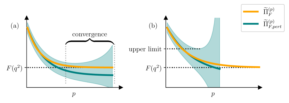
In the usual LCSR method using the Borel transformation, these expressions correspond to the limit . The relations we have derived thus far in this section are exact, but of little use without the knowledge of the correlation function to all orders in perturbation theory. In practice, we can only approximate the correlation function with a perturbatively calculated expression, as detailed in Section 2.2. The difference between the ’true’ and perturbative expressions of the correlation function originates from the truncation of the multiple perturbative expansions performed to obtain . This truncation error grows as increases because both the higher order LCOPE and hard QCD corrections become large, as we discuss in the next section. We plot schematically this behaviour in Fig.1. Our strategy is the following: we quantify the -dependent truncation error in Section 3.2 with a conservative order of magnitude estimate such that within uncertainties for all . Necessarily, when becomes too large, the estimated uncertainty diverges, and the calculation loses its predictive power. We claim that if the truncation error is not too large at large useful information can be extracted from LCSRs without QHD.
In fact, when increases there are two possible outcomes:
-
(a)
The continuum integral becomes negligible compared to and to the total error on before the latter diverges. We call this regime ’convergence of the sum rule’ (see Fig.1 (a)). In this case, we obtain a prediction of the form factor which does not require the knowledge of . In order to know that we have reached this regime, there are two criteria we can use without relying on the QHD approximation:
-
•
If truncation errors are small enough and the error is dominated by the LCDAs inputs then and become weakly dependent on and near the convergence.
-
•
In Eq. (3.5) is not an input of the mass sum rule, it is a genuine prediction of the meson mass from first principles. Usually, this relation is used to set the effective threshold in QHD [44], instead we use it as a criterion of convergence. A Taylor expansion of Eq. (3.7) yields
(3.10) hence, assuming that does not plateau before going to zero, the convergence of is a proxy for the quality of the convergence of the sum rule.
In this regime, attempting to estimate a negligible with QHD might introduce a systematic error that can be larger than the actual size of .
-
•
-
(b)
The error in the correlation function diverges before reaching the regime described above (see Fig.1 (b)). In this situation we can use the semi-local quark-hadron duality to determine the sign of for all considered using daughter sum rules to estimate the effective thresholds. From this information we can deduce an upper or lower limit on . In practice, we find in most cases, and in the few cases where the corresponding lower limits are negative, hence we focus on upper limits only. In principle, these upper limits are robust results since we rely on QHD solely to test the sign of . While not as compelling as predictions, these upper limits on local form factors can be useful in certain contexts. For example, smaller SM predictions for would reduce the tension between the experimental measurements and the SM predictions of . The determination of upper limits with sum rules is not a new idea. It has already been considered in the case of QCD sum rule, where the spectral density is positive definite. This consideration has been applied in the prediction of LCDA parameters, as documented in [48], as well as in the determination of decay constants, as discussed in [49, 50].
In order for this approach to yield useful results, we need a conservative yet accurate estimation of the truncation error. We detail our estimation of the perturbative error in in Section 3.2 and present our numerical results in Section 4. In this work we apply this method to -meson LCSRs but the same strategy can be applied to LCSRs with light-meson LCDAs as shown in Appendix C. The advantage of -meson LCSRs over light-meson LCSRs is the large number of form factors accessible with a single calculation, this allows us to check our results against numerous other works.
3.2 Perturbative error in
In this section, we estimate the uncertainties associated with the truncations of all perturbative expansions in the expression of . Our strategy is to write a parametric expression of the true correlation function in terms of the perturbative expression and unknown parameters whose prior we establish conservatively. Schematically we write , where is the estimated size of the correction and is a parameter of order one.
3.2.1 Fock state expansion in n-particle contributions
We perform the calculation up to -particle contributions. We define such that
| (3.11) |
Numerically we check that for the values of taken in consideration, which is in line with the results of [42]. We choose to be uniformly distributed in , which we deem conservative since the truncated terms are suppressed in the -particle expansion.
3.2.2 Radiative corrections in
In Section 2.2, we discussed the kinematic conditions for the interpolating quark to be highly virtual and for the radiative QCD corrections to remain small, and found . We define the average value of as
| (3.12) |
where is the integrand of the th derivative of the perturbative correlation function (2.9)
| (3.13) |
For , is of the order of a few GeV2, and when , . To estimate the size of the radiative correction, we define the characteristic scale
| (3.14) |
For a given renormalisation scheme, the correlation function expanded to all orders in perturbative QCD can be written as
| (3.15) |
where and . We choose to work in the renormalisation scheme and set . Setting to be of order and independent of the scale gives a crude yet conservative estimation of the QCD error when . Radiative corrections at NLO have been calculated for -meson LCDAs in SCET in [39]. In that work the Borel parameter is set to and the authors find that the largest radiative corrections are of order . Recalling that and setting the scale our estimation of the missing radiative correction is . Hence, we choose as a conservative interval for . In the mass sum rule (3.5) we make the conservative assumption that radiative corrections are uncorrelated between different derivatives.
3.2.3 LCOPE truncation error
We now focus on assessing the error arising from truncating the LCOPE. Matching the twist expansion of the LCDAs with that of the LCOPE, in the case of 2-particle LCDAs, the leading twists (LT) and contribute at order , while the next-to-leading twists (NLT) and contribute at order , and so forth. For -particle contributions, the twist counting starts at . Schematically we have
| (3.16) |
Additionally, the LCDAs are expanded within HQET. As well known, the power expansion in HQET is mismatched with the expansion in twists, hence the power counting in HQET is ill-defined at a given order in the twist expansion. However, we know that order in the LCOPE expansion corresponds to order in HQET, which can be seen e.g. from Eq. (2.14). We include 2-particle -meson LCDAs up to twist-5, thus encompassing the entire order of HQET. For 3-particle LCDAs, we only consider contributions up to twist-3 and twist-4, which correspond to the leading order contribution in the LCOPE and leading power in HQET. At the leading order in QCD, the propagator of the interpolating quark is exact at all orders in HQET, hence the order is fully included at QCD leading order in the 2-particle contributions. We do not account for the effect of higher power corrections which we expect to be negligible compared to the other errors we take into account. Following the expansion in made explicit in (3.16) we estimate the contribution from the missing twists by
| (3.17) |
where is a uniformly distributed parameter in the range . We also ensure that . At large and small one can show that is weakly dependent on . We use that approximation of -independent in the mass sum rule (3.5). From the expression Eq. (3.13), one can infer how the quality of the LCOPE is regulated by and . In Eq. (3.13) the leading twist contribute to and next-to-leading twist contribute to . Hence the ratio of two successive terms in (3.13) roughly corresponds to the ratio of next-to-leading twist over leading twist contributions. This ratio goes like , which in the limit of and goes like . This qualitatively shows how and the Borel parameter regulates the goodness of the LCOPE.
3.2.4 Total error model
Combining Eqs. (3.11), (3.15) and (3.17), we obtain the following expression for the exact correlation function
| (3.18) | ||||
We treat as nuisance parameters in a frequentist inference to account for the total error from perturbation theory. Based on the discussion above, we assume that they are uniformly distributed in the following ranges:
| (3.19) |
In this simplified model, as increases, the estimated uncertainty on becomes out of control because of the simultaneous decrease of towards zero and the increase of towards unity.
4 Numerical Results
4.1 Input parameters
We take meson masses from [51], while the remaining input parameters are listed in Table 2. The running of in the renormalisation scheme is performed using the package rundec [52].
| Parameters | Values | Ref. |
| Decay constants | MeV | [53] |
| MeV | [53] | |
| MeV | [53] | |
| MeV | [53] | |
| MeV | [46] | |
| MeV | [46] | |
| MeV | [49] | |
| QCD coupling | [51] | |
| Quark masses | [54] | |
| [54] | ||
| LCDA parameters | GeV2 | [55] |
| GeV2 | [55] | |
| [56]∗ |
The -LCDAs parameters have thus far solely been computed using QCD sum rules, and suffer from significant uncertainties. For and we use the estimation from [55], however a more recent prediction using a different sum rule finds a discrepant result [48], using these values instead yields a difference in the prediction of the form factors. The inverse moment of the -meson distribution amplitude has been derived using a QCD sum rule in [56] using two different models of quark-antiquark vacuum fluctuations. Each of these predictions comes with a normally distributed error. The authors provide a combination of these results as a normally distributed . In order to keep the normally distributed, we perform our own combination.
We work in a frequentist inference and sample our expression for from Eq.(3.18) with randomly drawn input parameters, including the error modeling parameters .
4.2 Prediction and upper limits on local form factors
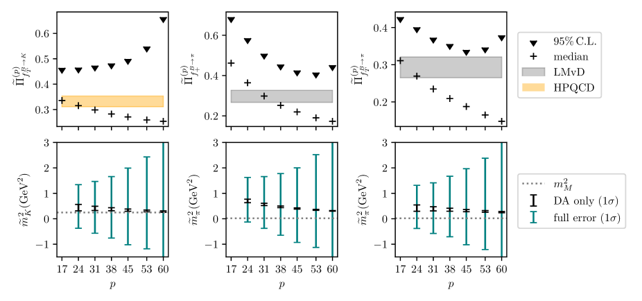
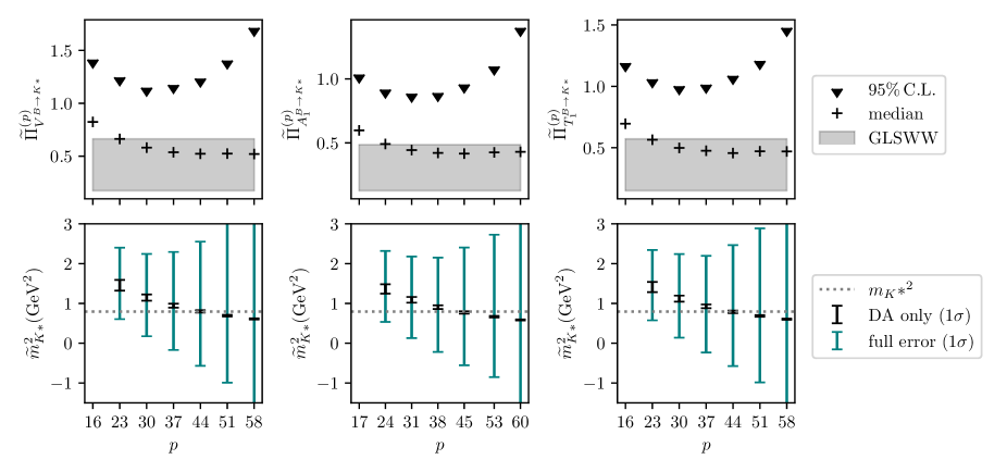
We present results for GeV2 which we find are representative values. We choose GeV2 as the minimal value which fulfills the QCD perturbativity condition (2.15). For GeV2 we encounter numerical limitations because of the large factorial entering . For each we increase until the error in starts diverging. We then go back and sample a large number of points for a few values of before the divergence. We illustrate this method in Fig. 2 for the form factor, and also includes the predictions from the mass sum rule and other relevant quantities. Similar figures are given in Appendix D for other form factors.
At , we restrict ourselves to a minimal basis for the form factors is reduced to , for pseudoscalar final mesons, and , , , and for vector final mesons. See Appendix A for their definitions. We present our results for upper bounds and predictions in Tables 3 and 4 for . The optimal values for the pair are chosen to obtain the most stringent upper limit at the confidence level for the considered form factor. We also present the median value and interval of the sampled at the said optimal pair. For all three values of , the optimal is searched in the interval where the scale GeV and the twist ratio is below .
We include in the tables an estimation of using QHD to test its sign and magnitude. The result one would obtain from the usual LCSR method is simply - . We use daughter sum rules to determine the effective thresholds in this case. For pseudo-Goldstone bosons, especially , daughter sum rules with -meson LCDAs tend to yield a smaller effective threshold than the equivalent QCD sum rule. In [42] the effective threshold for those processes was taken from the equivalent QCD sum rule due to this oddity in the daughter sum rule, which was deemed unreliable. We do not adopt the same strategy, since we are out of the windows for the Borel parameter which were used to determine the latter.
For we do not obtain viable results for two reasons. First, the NLT contribution is much larger, due to the large mass of the charm quark, which makes the error large before reaching the convergence. Secondly, the daughter sum rules do not work, preventing us from evaluating and checking its positivity.
The central values of can be used as indications for the predictions of the form factors assuming the convergence of the sum rule. We discuss convergence further in section 4.3. We find that all predictions are compatible with the literature albeit the uncertainties are rather large. The large error in our predictions, and the elevated values of the upper limits are due to the large uncertainties coming from the estimation of the perturbative error detailed in Eq. (3.18). This demonstrates the necessity of a more accurate assessment of the radiative corrections and the higher twist contributions, which would allow us to go at a larger number of derivation and get closer to the convergence and/or reduce the theoretical error.
From the three models introduced in Appendix B, the results in Tables 3 and 4 were obtained with the exponential model. It yields smaller yet compatible values compared to the local duality models A and B, with relative differences ranging from to . These models are asymptotically identical at low momentum, hence in the limit there is no difference between them.
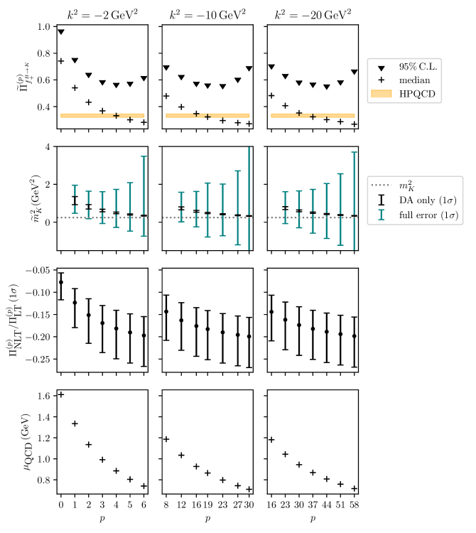
- row: percentile and median value of , . The orange bands represent the interval predicted by the HPQCD collaboration [24].
- row: black (orange) error bars: intervals including all errors (parametric error only). Dotted line: experimental value of .
- row: intervals of the ratio of next-to-leading twist over leading twist contributions.
- row: energy scale used for the estimation of the error from missing radiative correction.
| form factor | upper limit @ C.L. | literature | Ref. | |||
| [42]† [39] [37] [57] | ||||||
| [42]† [39] [37] [57] | ||||||
| [24] [42]† [39] [37] | ||||||
| [24] [42]† [37] [39] |
| form factor | upper limit @ C.L. | literature | Ref. | |||
| [42] [58] [46] | ||||||
| [42] [58] [46] | ||||||
| [42] | ||||||
| [42] [46] | ||||||
| - | [42] [46] | |||||
| [42] [58] [46] | ||||||
| [42] [58] [46] | ||||||
| [42] | ||||||
| [42] [58] [46] | ||||||
| - | [42] [58] [46] |
4.3 Convergence of the sum rule
The first criterion of convergence discussed in section 3.1 is the independence of the prediction w.r.t. and . At this stage, we find that it is the case within uncertainties, but this is rather meaningless given how large the latter are. The second criterion of convergence we examined is the convergence of . Similarly to the convergence of the form factor, taken at face value the total uncertainty on mass predictions is very large and thus mass predictions are not very useful at this stage to characterise convergence. They are dominated by our QCD error estimation, and computing the radiative corrections should reduce this uncertainty by a fair amount, and allow us to check the convergence of the sum rule.
So far the behaviour we have described was expected. However, we make an interesting observation in the mass sum rule. As shown in Fig.2, the value of including parametric errors only becomes remarkably close to the squared meson mass as increases, with very small parametric uncertainties. This is also true for and for all the form factors for and transitions as shown in Appendix D. We checked numerically that there is no correlation between the input parameter and the calculated . It is a truly surprising finding given how large the estimated error is. At this stage, this appears to be a numerical coincidence which has two possible explanations. Either the actual radiative corrections and higher twists contributions are small, or more probably, they cancel out in the ratio (3.5). In any case, such a quick and accurate convergence seems to be a sign that for a relatively large where the radiative corrections (although potentially large) are calculable perturbatively for .
The case of is different. In -meson LCSRs the breaking effects are very small at leading order in QCD, hence the mass sum rule yields . We expect that the radiative corrections break strongly to adjust the predicted mass of the pion. Notably, the corrections should be larger for since the first resonance of the pion spectral density is lighter than the first resonance of the kaon, and thus converges more slowly than .
As a check, the estimated values of including QCD and LCOPE truncation error are also reported for each form factor. Assuming QHD, it allows us to infer whether we can impose an upper limit by checking the positivity of . It also gives an indication of how far we are from the convergence of the sum rule since we expect to go to zero in this limit. We find that for every prediction is much smaller than the central value of the form factors, indicating that we are close to convergence.
4.4 Range of the Borel parameter
In Fig. 2, our results are plotted for three different values of with the x-axis spanning the corresponding optimal ranges of . From this figure, one can easily see that is weakly dependent on the ratio . This is true for each form factor we studied. This shows that the Borel transformation converges very quickly and the paramount quantity to assess the quality of the LCOPE is -as expected- the ratio . As noted earlier, taking for a finite is equivalent to taking after a Borel transformation, and is known to correspond to a complete suppression of the continuum, but breaks the LCOPE.
That being said, avoiding the Borel transformation comes with two advantages. First, the convergence criteria we introduced in Section 3.1 include the independence of on both and independently. This is a more stringent condition than the independence on their ratio only used the traditional LCSR approach (see e.g. [43]). The second advantage of keeping an explicit dependence on and is that the convergence is sometimes better at low (although marginally) than at larger where we recover the result of the Borel transformation. This is illustrated in Table 3 for the form factors.
From the Tables 3 and 4, one can see that the ratios we take for our upper bounds are somewhat small compared to the usual range prescribed for the Borel parameters. Typically, one expects GeV2 for [30]. These ranges have been established from two-point sum rules in the light meson channel [47, 43] and LCSRs with the pion distribution amplitude [59, 60, 61]. They stem from the usual compromise between the suppression of the spectral density integral and truncation errors, typically allowing to be as large as of , while keeping the truncated contribution smaller than of .
In our approach, we reevaluate these intervals with a different goal in mind. We allow larger (yet conservatively estimated) truncation errors in order to better suppress the spectral density integral, and thus we settle on GeV2, a bit lower than the usually considered Borel window. This is possible because there is a disconnect between and the average virtuality in this limit, e.g. in Fig. 2 the point GeV2 and corresponds to GeV2, larger than the expected GeV2.
4.5 Correlation between form factors
Since the core result of -meson LCSRs relies on the same shared LCDA parameters for all form factors, we expect this calculation to yield strongly correlated predictions. Moreover, for a given form factor the correlation function is the same for different processes up to the interpolating quark mass. We show an example of this effect in Fig.3. The correlation between form factors predicted using -meson LCSRs is usually hampered by the determination of the Borel parameter and effective threshold which have a relatively large uncertainty and are a priori uncorrelated between different decays. Since we avoid QHD in our procedure we can recover a strong correlation between all predicted form factors, as long as the uncertainty coming from -meson LCDAs dominates. A large part of the uncertainty in our current calculation originates from perturbative QCD, which dilutes the correlations for now.
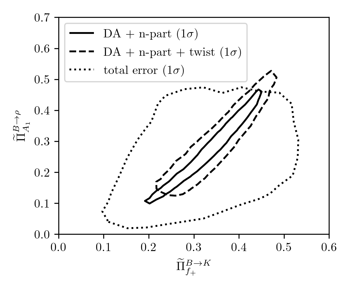
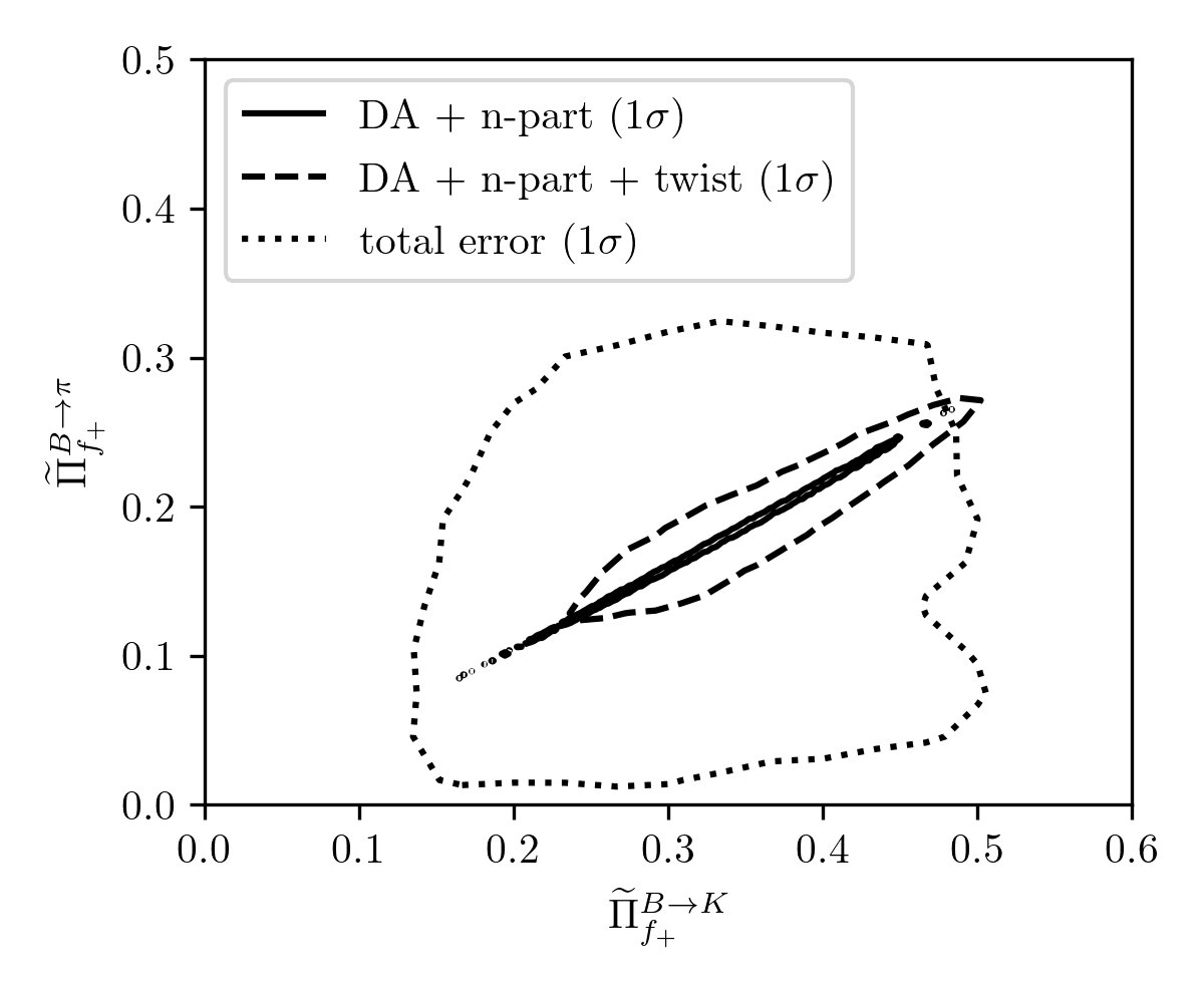
In Fig. 3 we show the confidence levels of our predictions in the planes and breaking down the different sources of error. When accounting for the total error, there is virtually no correlation between our predictions, which is expected because of the large and uncorrelated QCD error. Removing the latter yields a strong correlation between our predictions, even when accounting for LCOPE truncation errors. Keeping only parametric errors we see even stronger correlations, reaching almost correlation between and which is expected at QCD LO for -meson LCSR. Even without improving our current knowledge of -meson distribution amplitudes, calculating the QCD radiative corrections to the correlator would significantly increase the statistical correlation between all predicted form factors. While the absolute size of the error would still be comparable to other calculations employing -meson LCDAs, this correlation can have strong phenomenological implications.
5 Conclusion
In this article, we propose a strategy to predict form factors using LCSRs without the QHD approximation, and thus without relying on the determination of an effective threshold and a window for the Borel parameter. Our approach consists in evaluating conservatively the truncation error in the correlator, and taking to be as small as possible in order to suppress the spectral density integral . We introduce two tests of the suppression of which do not rely on QHD, namely the - and -independence of the predicted form factors, and the convergence of the mass sum rule towards the physical value of the squared meson mass . Our approach reduces greatly the systematic uncertainty associated to the LCSR method. However, this improvement comes at the cost of a larger dependence on higher-order perturbative corrections. This trade-off is advantageous, since these corrections are calculable. The other notable advantage of this method is that in -meson LCSRs it predicts strongly correlated form factors between different processes.
Using a conservative model of the error in we find that can be taken a bit below the canonical GeV2 Borel window, thanks to the fact that a direct assessment of the average virtuality yields higher values than the approximation and thus hints at smaller expected radiative corrections. At this stage, an assessment of the convergence of the sum rule in this regime is hampered by the relatively large truncation error which affects both and . However, we find that without the modeled truncation error, converges remarkably fast and accurately to the physical values of for . Our understanding of this observation is that converges quickly to zero and the missing perturbative corrections cancel out in the ratio in the mass sum rule provided in Eq. (3.5). In this case, computing the NLO QCD correction could allow us to demonstrate the convergence in the region GeV2. In addition, the knowledge of these radiative corrections would lead to highly correlated predictions of the form factors.
Interestingly, the same method can be applied to LCSRs with light-meson LCDAs and should prove to perform better. Indeed, the light-meson LCDAs are generally better known, with smaller parametric uncertainties [31]. They do not exhibit UV divergences similar to the one mentioned in section 2.4. Furthermore, for the and transitions, the contributions from the highest known twists have been shown to be negligible [36, 37], hence indicating that the LCOPE should be under control at small in our approach. For each form factor considered in this work, the NLO QCD corrections have already been calculated in LCSRs with light-meson LCDAs [28, 31, 46, 41], at least for the leading twists contributions. It would be interesting to compare the results of this method applied with light-meson LCDAs to the ones already obtained with the usual procedure. Light-meson LCDAs also present the advantage of enabling exploration of higher values of , surpassing the restriction .
Acknowledgement:
The authors are grateful to A. Khodjamirian, T. Hurth and D. van Dyk for useful comments. The work of A.C. was supported in part by the National Research Agency (ANR) under project ANR-21-CE31-0002-01, and in part by the Italian Ministry of University and Research under the grant 2022N4W8WR.
Appendix A Definition of local hadronic form factors
The relevant form factors for the transitions, with are , and . We define:
| (A.1) | ||||
For transitions, with , we consider , , , , , and , which can be defined with:
| (A.2) | ||||
where denotes the momentum of the -meson, that of the light meson and is the momentum transfer, while stands for the polarisation of the vector meson. We work in the convention. We also introduce the form factor combination as in [42], motivated by its easy extraction directly from a sum rule. It is defined as
| (A.3) |
We work at , at which there are extra relations between the different form factors:
| (A.4) | ||||
We also define as
| (A.5) |
where is the Källén function. At this reduces to
| (A.6) |
Appendix B -meson distribution amplitudes
| (B.1) |
| (B.2) |
The brackets and such denote Wilson lines that render the LCDAs gauge invariant. We work in the Fock-Schwinger gauge where the Wilson lines are 1, and adopt again the convention .
While the 3-particle -LCDAs basis in (B) has the advantage of having simple Lorentz structures, for LCSRs it is more convenient to work in a basis of LCDAs with definite collinear twists
| (B.3) | |||
For both 2-particle and 3-particle LCDAs we consider all three models given in [45], namely the exponential and the two local-duality models: local duality A, and local duality B. Only the Wandzura-Wilczek approximation was given for in [42], as the full LCDA depends on , which also lacked a specified model. More recently models for the exponential model and the local-duality B one were given for in [58]. A general ansätz was later derived in [39] that we use to obtain an expression for all three models. We check that we are in agreement with [58].
For the complete expression of , following [45] we start from the equation
| (B.4) |
where
| (B.5) |
and
| (B.6) |
This yields
| (B.7) |
Exponential Model:
| (B.8) | |||
| (B.9) |
This result is obtained with the following Grozin-Neubert constraints
| (B.10) |
Local duality A:
| (B.11) | |||
| (B.12) |
This result is obtained with the following Grozin-Neubert constraints
| (B.13) |
Local duality B:
| (B.14) | |||
| (B.15) |
This result is obtained with the following Grozin-Neubert constraints
| (B.16) |
Appendix C Light-meson LCDAs
For LCSRs with light-meson LCDAs, the starting point is a vacuum to light-meson correlation function [27, 28]:
| (C.1) |
where is the relevant weak current, and is the interpolating field for the -meson.
This time, the -meson of momentum is off-shell while the light-meson is on-shell. Once again, the correlation function can be rewritten using analyticity and the unitary relation, and then further expressed as a sum of scalar functions times a Lorentz structure. Scalar relations are extracted in the form
| (C.2) |
On the perturbative side, it takes the expression :
| (C.3) |
The method presented in this article is applicable to the correlation function with light-meson LCDAs, and since similarly and , we derive the analogous relations
| (C.4) |
And the corollary is
| (C.5) |
Appendix D Additional figures for and
In this section we plot our numerical results for and near the breakdown of the LCOPE for , , .

References
- [1] LHCb collaboration, R. Aaij et al., Test of lepton universality with decays, JHEP 08 (2017) 055, [1705.05802].
- [2] LHCb collaboration, R. Aaij et al., Test of lepton universality in beauty-quark decays, Nature Phys. 18 (2022) 277–282, [2103.11769].
- [3] LHCb collaboration, R. Aaij et al., Measurement of lepton universality parameters in and decays, Phys. Rev. D 108 (2023) 032002, [2212.09153].
- [4] LHCb collaboration, R. Aaij et al., Measurement of Form-Factor-Independent Observables in the Decay , Phys. Rev. Lett. 111 (2013) 191801, [1308.1707].
- [5] LHCb collaboration, R. Aaij et al., Differential branching fractions and isospin asymmetries of decays, JHEP 06 (2014) 133, [1403.8044].
- [6] LHCb collaboration, R. Aaij et al., Differential branching fraction and angular analysis of decays, JHEP 06 (2015) 115, [1503.07138].
- [7] LHCb collaboration, R. Aaij et al., Angular analysis and differential branching fraction of the decay , JHEP 09 (2015) 179, [1506.08777].
- [8] LHCb collaboration, R. Aaij et al., Angular analysis of the decay using 3 fb-1 of integrated luminosity, JHEP 02 (2016) 104, [1512.04442].
- [9] LHCb collaboration, R. Aaij et al., Measurement of -Averaged Observables in the Decay, Phys. Rev. Lett. 125 (2020) 011802, [2003.04831].
- [10] LHCb collaboration, R. Aaij et al., Angular Analysis of the Decay, Phys. Rev. Lett. 126 (2021) 161802, [2012.13241].
- [11] LHCb collaboration, R. Aaij et al., Angular analysis of the rare decay , JHEP 11 (2021) 043, [2107.13428].
- [12] LHCb collaboration, R. Aaij et al., Branching Fraction Measurements of the Rare and - Decays, Phys. Rev. Lett. 127 (2021) 151801, [2105.14007].
- [13] CMS collaboration, A. Hayrapetyan et al., Test of lepton flavor universality in B± K and B± K±e+e- decays in proton-proton collisions at = 13 TeV, 2401.07090.
- [14] C. Bobeth, M. Chrzaszcz, D. van Dyk and J. Virto, Long-distance effects in from analyticity, Eur. Phys. J. C 78 (2018) 451, [1707.07305].
- [15] N. Gubernari, D. van Dyk and J. Virto, Non-local matrix elements in , JHEP 02 (2021) 088, [2011.09813].
- [16] S. Jäger and J. Martin Camalich, On at small dilepton invariant mass, power corrections, and new physics, JHEP 05 (2013) 043, [1212.2263].
- [17] S. Jäger and J. Martin Camalich, Reassessing the discovery potential of the decays in the large-recoil region: SM challenges and BSM opportunities, Phys. Rev. D 93 (2016) 014028, [1412.3183].
- [18] M. Ciuchini, M. Fedele, E. Franco, S. Mishima, A. Paul, L. Silvestrini et al., decays at large recoil in the Standard Model: a theoretical reappraisal, JHEP 06 (2016) 116, [1512.07157].
- [19] B. Capdevila, S. Descotes-Genon, L. Hofer and J. Matias, Hadronic uncertainties in : a state-of-the-art analysis, JHEP 04 (2017) 016, [1701.08672].
- [20] V. G. Chobanova, T. Hurth, F. Mahmoudi, D. Martinez Santos and S. Neshatpour, Large hadronic power corrections or new physics in the rare decay ?, JHEP 07 (2017) 025, [1702.02234].
- [21] A. Arbey, T. Hurth, F. Mahmoudi and S. Neshatpour, Hadronic and New Physics Contributions to Transitions, Phys. Rev. D 98 (2018) 095027, [1806.02791].
- [22] M. Ciuchini, A. M. Coutinho, M. Fedele, E. Franco, A. Paul, L. Silvestrini et al., Hadronic uncertainties in semileptonic decays, PoS BEAUTY2018 (2018) 044, [1809.03789].
- [23] M. Bordone, G. isidori, S. Mächler and A. Tinari, Short- vs. long-distance physics in : a data-driven analysis, 2401.18007.
- [24] (HPQCD collaboration)§, HPQCD collaboration, W. G. Parrott, C. Bouchard and C. T. H. Davies, B→K and D→K form factors from fully relativistic lattice QCD, Phys. Rev. D 107 (2023) 014510, [2207.12468].
- [25] A. Khodjamirian and R. Ruckl, QCD sum rules for exclusive decays of heavy mesons, Adv. Ser. Direct. High Energy Phys. 15 (1998) 345–401, [hep-ph/9801443].
- [26] V. M. Braun, QCD sum rules for heavy flavors, PoS hf8 (1999) 006, [hep-ph/9911206].
- [27] P. Ball and R. Zwicky, decay form-factors from light-cone sum rules revisited, Phys. Rev. D 71 (2005) 014029, [hep-ph/0412079].
- [28] P. Ball and R. Zwicky, New results on decay formfactors from light-cone sum rules, Phys. Rev. D 71 (2005) 014015, [hep-ph/0406232].
- [29] A. Khodjamirian, T. Mannel and N. Offen, B-meson distribution amplitude from the form-factor, Phys. Lett. B 620 (2005) 52–60, [hep-ph/0504091].
- [30] A. Khodjamirian, T. Mannel and N. Offen, Form-factors from light-cone sum rules with B-meson distribution amplitudes, Phys. Rev. D 75 (2007) 054013, [hep-ph/0611193].
- [31] G. Duplancic, A. Khodjamirian, T. Mannel, B. Melic and N. Offen, Light-cone sum rules for form factors revisited, JHEP 04 (2008) 014, [0801.1796].
- [32] G. Duplancic and B. Melic, B, B(s) — K form factors: An Update of light-cone sum rule results, Phys. Rev. D 78 (2008) 054015, [0805.4170].
- [33] A. Khodjamirian, T. Mannel, A. A. Pivovarov and Y. M. Wang, Charm-loop effect in and , JHEP 09 (2010) 089, [1006.4945].
- [34] A. Bharucha, Two-loop Corrections to the Form Factor from QCD Sum Rules on the Light-Cone and , JHEP 05 (2012) 092, [1203.1359].
- [35] Y.-M. Wang and Y.-L. Shen, QCD corrections to B→ form factors from light-cone sum rules, Nucl. Phys. B 898 (2015) 563–604, [1506.00667].
- [36] A. V. Rusov, Higher-twist effects in light-cone sum rule for the form factor, Eur. Phys. J. C 77 (2017) 442, [1705.01929].
- [37] A. Khodjamirian and A. V. Rusov, and decays at large recoil and CKM matrix elements, JHEP 08 (2017) 112, [1703.04765].
- [38] C.-D. Lü, Y.-L. Shen, Y.-M. Wang and Y.-B. Wei, QCD calculations of form factors with higher-twist corrections, JHEP 01 (2019) 024, [1810.00819].
- [39] B.-Y. Cui, Y.-K. Huang, Y.-L. Shen, C. Wang and Y.-M. Wang, Precision calculations of Bd,s → , K decay form factors in soft-collinear effective theory, JHEP 03 (2023) 140, [2212.11624].
- [40] N. Gubernari, A. Khodjamirian, R. Mandal and T. Mannel, and form factors from QCD light-cone sum rules, JHEP 12 (2023) 015, [2309.10165].
- [41] A. Khodjamirian, B. Melić and Y.-M. Wang, A guide to the QCD light-cone sum rule for -quark decays, 2311.08700.
- [42] N. Gubernari, A. Kokulu and D. van Dyk, and Form Factors from -Meson Light-Cone Sum Rules beyond Leading Twist, JHEP 01 (2019) 150, [1811.00983].
- [43] P. Colangelo and A. Khodjamirian, QCD sum rules, a modern perspective, in At the frontier of particle physics. Handbook of QCD. Vol. 1-3 (M. Shifman and B. Ioffe, eds.), pp. 1495–1576. World Scientific, Singapore, 10, 2000. hep-ph/0010175.
- [44] A. Khodjamirian, Hadron Form Factors: From Basic Phenomenology to QCD Sum Rules. CRC Press, Taylor & Francis Group, Boca Raton, FL, USA, 2020.
- [45] V. M. Braun, Y. Ji and A. N. Manashov, Higher-twist B-meson Distribution Amplitudes in HQET, JHEP 05 (2017) 022, [1703.02446].
- [46] A. Bharucha, D. M. Straub and R. Zwicky, in the Standard Model from light-cone sum rules, JHEP 08 (2016) 098, [1503.05534].
- [47] M. A. Shifman, A. I. Vainshtein and V. I. Zakharov, QCD and Resonance Physics. Theoretical Foundations, Nucl. Phys. B 147 (1979) 385–447.
- [48] M. Rahimi and M. Wald, QCD sum rules for parameters of the B-meson distribution amplitudes, Phys. Rev. D 104 (2021) 016027, [2012.12165].
- [49] P. Gelhausen, A. Khodjamirian, A. A. Pivovarov and D. Rosenthal, Decay constants of heavy-light vector mesons from QCD sum rules, Phys. Rev. D 88 (2013) 014015, [1305.5432].
- [50] A. Khodjamirian, Upper bounds on f(D) and f(D(s)) from two-point correlation function in QCD, Phys. Rev. D 79 (2009) 031503, [0812.3747].
- [51] Particle Data Group collaboration, R. L. Workman and Others, Review of Particle Physics, PTEP 2022 (2022) 083C01.
- [52] F. Herren and M. Steinhauser, Version 3 of RunDec and CRunDec, Comput. Phys. Commun. 224 (2018) 333–345, [1703.03751].
- [53] Flavour Lattice Averaging Group (FLAG) collaboration, Y. Aoki et al., FLAG Review 2021, Eur. Phys. J. C 82 (2022) 869, [2111.09849].
- [54] J. Aebischer, J. Kumar and D. M. Straub, Wilson: a Python package for the running and matching of Wilson coefficients above and below the electroweak scale, Eur. Phys. J. C 78 (2018) 1026, [1804.05033].
- [55] T. Nishikawa and K. Tanaka, QCD Sum Rules for Quark-Gluon Three-Body Components in the B Meson, Nucl. Phys. B 879 (2014) 110–142, [1109.6786].
- [56] A. Khodjamirian, R. Mandal and T. Mannel, Inverse moment of the Bs-meson distribution amplitude from QCD sum rule, JHEP 10 (2020) 043, [2008.03935].
- [57] D. Leljak, B. Melić and D. van Dyk, The → form factors from QCD and their impact on —Vub—, JHEP 07 (2021) 036, [2102.07233].
- [58] J. Gao, C.-D. Lü, Y.-L. Shen, Y.-M. Wang and Y.-B. Wei, Precision calculations of form factors from soft-collinear effective theory sum rules on the light-cone, Phys. Rev. D 101 (2020) 074035, [1907.11092].
- [59] V. M. Braun, A. Khodjamirian and M. Maul, Pion form-factor in QCD at intermediate momentum transfers, Phys. Rev. D 61 (2000) 073004, [hep-ph/9907495].
- [60] V. M. Braun and I. E. Halperin, Soft contribution to the pion form-factor from light cone QCD sum rules, Phys. Lett. B 328 (1994) 457–465, [hep-ph/9402270].
- [61] A. Khodjamirian, Form-factors of gamma* rho — pi and gamma* gamma — pi0 transitions and light cone sum rules, Eur. Phys. J. C 6 (1999) 477–484, [hep-ph/9712451].