Supplementary Information for “Beyond Linear Response: Equivalence between Thermodynamic Geometry and Optimal Transport”

I Optimal transport formulation of optimal, work-minimizing protocols

We present a concise derivation the optimal transport formulation of minimum-work protocols. For simplicity here we use the notation $\rho_{t}=\rho(\cdot,t)$ and $U_{t}=U_{\lambda(t)}(\cdot)$. For now, we consider the initial conditions $\rho_{0}=\rho_{i}^{\mathrm{eq}}$ and $U_{0}=U_{i}$, and the terminal condition $U_{\tau}=U_{f}$, without imposing $\rho_{\tau}=\rho_{f}^{\mathrm{eq}}$.

Recall that the Fokker-Planck equation giving the time-evolution for $\rho_{t}$ may be written as the continuity equation

$$\frac{\partial\rho_{t}}{\partial t}=\nabla\cdot(\rho_{t}\nabla\phi_{t}),\quad\quad\mathrm{where}\quad\quad\phi_{t}:=U_{t}+\ln\rho_{t}.$$ (S1)

The ensemble work rate is defined as

$$\frac{{\mathrm{d}}W}{{\,\mathrm{d}t}}=\int\rho_{t}(x)\,\frac{{\mathrm{d}}U_{t}(x)}{{\,\mathrm{d}t}}{\,\mathrm{d}x}.$$ (S2)

By applying the identity $\frac{{\mathrm{d}}}{{\,\mathrm{d}t}}\int\rho_{t}\,U_{t}{\,\mathrm{d}x}=\int(\partial_{t}\rho_{t})\,U_{t}{\,\mathrm{d}x}+\int\rho_{t}\,(\partial_{t}U_{t}){\,\mathrm{d}x}$ fir , algebraic manipulation yields

$$\frac{{\mathrm{d}}W}{{\,\mathrm{d}t}} =-\int\frac{\partial\rho_{t}}{\partial t}\,U_{t}{\,\mathrm{d}x}+\frac{{\mathrm{d}}}{{\,\mathrm{d}t}}\int\rho_{t}\,U_{t}{\,\mathrm{d}x}$$

$$=-\int\frac{\partial\rho_{t}}{\partial t}\,(U_{t}+\ln\rho_{t}+1){\,\mathrm{d}x}+\frac{{\mathrm{d}}}{{\,\mathrm{d}t}}\int\rho_{t}\,(U_{t}+\ln\rho_{t}){\,\mathrm{d}x}$$

$$=\int\rho_{t}|\nabla(U_{t}+\ln\rho_{t})|^{2}{\,\mathrm{d}x}+\frac{{\mathrm{d}}}{{\,\mathrm{d}t}}\int\rho_{t}\,(U_{t}+\ln\rho_{t}){\,\mathrm{d}x}.$$ (S3)

Here in the second line we have added and subtracted $\frac{{\mathrm{d}}}{{\,\mathrm{d}t}}\int\rho_{t}\ln\rho_{t}{\,\mathrm{d}x}=\int(\partial_{t}\rho_{t})(\ln\rho_{t}+1){\,\mathrm{d}x}$, and in the third line we have plugged in the Fokker-Planck equation Eq. (S1) and integrated by parts in $x$.

Finally, the work is defined as the time-integral of the work rate

$$W=\int_{0}^{\tau}\frac{{\mathrm{d}}W}{{\,\mathrm{d}t}}{\,\mathrm{d}t}=\int_{0}^{\tau}\int\rho_{t}|\nabla\phi_{t}|^{2}{\,\mathrm{d}x}{\,\mathrm{d}t}+\int\rho_{t}(U_{t}+\ln\rho_{t}){\,\mathrm{d}x}\bigg{|}_{t=0}^{\tau},$$ (S4)

where we have used the definition of $\phi_{t}$ in Eq. (S1).

After noting that the KL divergence from a distribution $\rho$ to another an equilibrium distribution $\rho^{\mathrm{eq}}_{\lambda}$ can be equivalently written as

$$D_{\mathrm{KL}}(\rho|\rho^{\mathrm{eq}}_{\lambda}) :=\int\rho(x)\,\ln\bigg{[}\frac{\rho(x)}{\rho^{\mathrm{eq}}_{\lambda}(x)}\bigg{]}{\,\mathrm{d}x}=\int\rho\,(\ln\rho+U_{\lambda}){\,\mathrm{d}x}-F(\lambda)$$ (S5)

(recall $F(\lambda):=-\ln\int\exp(-U_{\lambda}(x)){\,\mathrm{d}x}$ is the equilibrium free energy), the excess work $W_{\mathrm{ex}}=W-\Delta F$ can be written as

$$W_{\mathrm{ex}}=\int_{0}^{\tau}\int\rho_{t}|\nabla\phi_{t}|^{2}{\,\mathrm{d}x}{\,\mathrm{d}t}+D_{\mathrm{KL}}(\rho_{\tau}|\rho_{f}^{\mathrm{eq}}),$$ (S6)

where we have applied the boundary conditions $\rho_{0}=\rho_{i}^{\mathrm{eq}},U_{0}=U_{i}$, and $U_{\tau}=U_{f}$.

The first term in Eq. (S6) represents the dissipation occurring within the protocol from $t=0$ and $t=\tau$ Ito (2024) and is optimized by a Benamou-Brenier solution between $\rho_{0}$ and $\rho_{\tau}$, while the second term represents the dissipation occurring for $t>\tau$ (i.e., after the protocol) as the distribution relaxes from $\rho_{\tau}$ to $\rho_{\infty}=\rho^{\mathrm{eq}}_{f}$. The change of variables $s=t/\tau$ thus yields $W_{\mathrm{ex}}^{*}=\min_{\rho_{f}}\mathcal{W}_{2}^{2}[\rho_{i}^{\mathrm{eq}},\rho_{f}]/\tau+D_{\mathrm{KL}}(\rho_{f}|\rho_{f}^{\mathrm{eq}})$, which was noted in Chen et al. (2019) to be equivalent to the JKO scheme used to study convergence properties of the Fokker-Planck equation Jordan et al. (1998) with effective time-step $h=\Delta t/2$.

If the additional terminal condition $\rho_{\tau}=\rho_{f}^{\mathrm{eq}}$ is additionally imposed, then the second KL divergence term goes away, reproducing the Benamou-Brenier cost function multiplied by $1/\tau$.

II Numerical study of linearly-biased double well optimal protocols

In this section, we provide details of our numerical study of the linearly-biased double well

$$U_{\lambda}(x)=E_{0}[(x^{2}-1)^{2}/4-\lambda x],$$ (S7)

for $E_{0}=16,\lambda_{i}=-1,\lambda_{f}=1$, and analyze the reduction in performance around $\tau\sim 2$ seen in Fig S1(a) (a higher resolution version of Fig. 2(e)). We propose an explanation for the geodesic-counterdiabatic protocols overshooting the optimal protocols (Fig S2(b)) that correspond to a reduction in performance for $\tau\sim 2$.

II.1 Lattice discretization implementation

In order to calculate $g(\lambda)$, $h(\lambda),\mathcal{T}^{2}(\lambda_{i},\lambda),D_{\mathrm{KL}}(\rho_{\lambda}^{\mathrm{eq}}|\rho_{f}^{\mathrm{eq}})$, as well as to measure the performance $W_{\mathrm{ex}}[\lambda(t)]$, we base our numerical implementation on the lattice-discretized Fokker-Planck equation method introduced in Holubec et al. (2019). This is the same discretization scheme used by Zhong and DeWeese (2022), which allows a direct comparison of numerical results.

We discretize the one-dimensional configuration space as an $N$-state lattice with spacing $\Delta x$ and reflecting boundaries at $x_{\mathrm{b}}=\pm(N-1)\Delta x/2$. Following Zhong and DeWeese (2022), we use $\Delta x=0.025$ and $x_{b}=\pm 3$. The probability density may be represented as a vector ${\bm{\rho}}(t)=(\rho^{1}(t),\rho^{2}(t),...,\rho^{N}(t))$ via $\rho(x,t)=(\Delta x)^{-1}[{\bm{\rho}}(t)]^{l(x)}$ , where $l(x)=\lfloor x/\Delta x+N/2\rfloor$. Likewise, the potential energy may be represented as a covector ${\bm{U}}_{\lambda}=(U_{1}(\lambda),U_{2}(\lambda),...,U_{N}(\lambda)))^{T}$ with $U_{\lambda}(x)=[{\bm{U}}_{\lambda}]_{l(x)}$, yielding the equilibrium probability vector ${\bm{\rho}}^{\mathrm{eq}}_{\lambda}=Z(\lambda)^{-1}(\exp(-U_{1}(\lambda)),\exp(-U_{2}(\lambda)),...,\exp(-U_{N}(\lambda)))$, where $Z(\lambda)=\sum_{i}\exp(-U_{i}(\lambda))$ is the normalization constant. The excess conjugate force is given by the covector

$$\bm{\delta f}(\lambda)=-\frac{\partial{\bm{U}}_{\lambda}}{\partial\lambda}+\frac{\partial{\bm{U}}_{\lambda}}{\partial\lambda}\cdot{\bm{\rho}}^{\mathrm{eq}}_{\lambda},$$ (S8)

where the second term is a dot product with the equilibrium probability vector.

The Fokker-Planck equation is represented as the master equation

$$\dot{{{\bm{\rho}}}}={\cal{L}}_{\lambda}{{\bm{\rho}}},$$ (S9)

where ${\cal{L}}_{\lambda}$ is a transition rate matrix on which we impose the following form

$${[{\cal{L}}_{\lambda}]^{i}}_{j}=\begin{cases}(\Delta x)^{-2}\ e^{(U_{j}(\lambda)-U_{i}(\lambda))/2}&{|i-j|=1}\\ -(\Delta x)^{-2}\ \sum_{k\neq j}\ e^{(U_{j}(\lambda)-U_{k}(\lambda))/2}&{i=j}\\ 0&\mathrm{else}.\end{cases}$$ (S10)

Taking the continuum limit $N\rightarrow\infty,\Delta x\rightarrow 0$ with constant $x_{\mathrm{b}}$ yields the Fokker-Planck equation $\partial_{t}\rho=\mathcal{L}_{\lambda}\rho$ Zhong and DeWeese (2022).

For this lattice discretization, The friction tensor and Fisher information metric are given by

$$g(\lambda)=-\sum_{i=1}^{N}[{\bm{\rho}}^{\mathrm{eq}}_{\lambda}]^{i}[\bm{\delta f}]_{i}\big{[}({\cal{L}}_{\lambda}^{T})^{-1}\bm{\delta f}\big{]}_{i}\quad\mathrm{and}\quad h(\lambda)=\sum_{i=1}^{N}[{\bm{\rho}}^{\mathrm{eq}}_{\lambda}]^{i}[\bm{\delta f}]_{i}[\bm{\delta f}]_{i},$$ (S11)

where $({\cal{L}}_{\lambda}^{T})^{-1}$ is the inverse of the adjoint Fokker-Planck matrix with its zero-mode removed Wadia et al. (2022). The KL-divergence is

$$D_{\mathrm{KL}}(\rho_{\lambda}^{\mathrm{eq}}|\rho_{f}^{\mathrm{eq}})=\sum_{i=1}^{N}[{\bm{\rho}}^{\mathrm{eq}}_{\lambda}]^{i}\,\ln\bigg{[}\frac{[{\bm{\rho}}^{\mathrm{eq}}_{\lambda}]^{i}}{[{\bm{\rho}}^{\mathrm{eq}}_{f}]^{i}}\bigg{]},$$ (S12)

and the squared thermodynamic distance (cf., Eq. (5) in Crooks (2007)) takes the form

$$\mathcal{T}^{2}(\lambda_{i},\lambda)=\bigg{[}\int_{\lambda_{i}}^{\lambda}\sqrt{g(\lambda)}\,{\mathrm{d}}\lambda\bigg{]}^{2}.$$ (S13)

We numerically compute the integral as a trapezoid sum on interval $[\lambda_{i},\lambda]$ split into 1000 even subintervals.

Geodesic-counterdiabatic protocols of duration $\tau$ are obtained by first solving for $\gamma_{f}$ through minimizing

$$\gamma_{f}=\arg\min_{\lambda}\ \mathcal{T}^{2}(\lambda_{i},\lambda)/\tau+D_{\mathrm{KL}}(\rho_{\lambda}^{\mathrm{eq}}|\rho_{f}^{\mathrm{eq}})$$ (S14)

using Eq. (S12) and (S13) above, and then computing the time-discretized geodesic for $k=0,1,2,...,K$

$$\gamma(\cdot)=\{(s_{0}=0,\gamma_{0}=\lambda_{i}),(s_{1},\gamma_{1}),(s_{2},\gamma_{2}),...,(s_{K-1},\gamma_{K-1}),(s_{K}=1,\gamma_{K}=\gamma_{f})\}$$ (S15)

using equally spaced $\gamma_{k}=[1-(k/K)]\lambda_{i}+(k/K)\gamma_{f}=\lambda_{i}+k\Delta\gamma$, and variable timesteps $s_{k+1}-s_{k}=\alpha\Delta\gamma\sqrt{g(\gamma_{k})+g(\gamma_{k+1})/2}$ with scaling factor $\alpha$ chosen so that $s_{K}=1$. Finally, the time-discretized $\eta(\cdot)$ is obtained via

$$\eta(s)=h^{-1}(\gamma(s))g(\gamma(s))\frac{{\mathrm{d}}\gamma(s)}{{\,\mathrm{d}s}}$$ (S16)

where ${\mathrm{d}}\gamma(s)/{\,\mathrm{d}s}$ is computed using finite differences.

Following Zhong and DeWeese (2022), we use $K=1000$. This way of computing geodesic-counterdiabatic protocols is consistent with how geodesic protocols were obtained in Zhong and DeWeese (2022), allowing for a direct comparison of performance.

II.2 Phase transition for $\gamma_{f}$

An interesting property we found for this problem is that the geodesic endpoint $\gamma_{f}$ obtained as the argmin of the objective function Eq. (S14) has a discontinuity at $\tau\approx 3.3$ (Fig. S2(a)). This is due to the fact that the objective function, computed using Eqs. (S11)-(S13), is not convex, and has multiple local minima for $\tau\sim 3$ (Fig. S2(b)).

II.3 Measuring performance

For a time-discretized protocol $\lambda(t)=\{(t_{0}=0,\lambda_{0}=\lambda_{i}),(t_{1},\lambda_{1}),...,(t_{K-1},\lambda_{K-1}),(t_{K}=\tau,\lambda_{K})\}$, the trajectory for ${\bm{\rho}}(t)$ is obtained by integrating Eq. (S9)

$${\bm{\rho}}_{k+1}=\exp[\mathcal{L}_{k+1/2}(t_{k+1}-t_{k})]\,{\bm{\rho}}_{k}\quad\mathrm{with}\quad{\bm{\rho}}_{0}={\bm{\rho}}_{i}^{\mathrm{eq}},$$ (S17)

where $\mathcal{L}_{k+1/2}$ is the transition rate matrix Eq. (S10) for $\lambda_{k+1/2}=(\lambda_{k}+\lambda_{k+1}/2)$.

Finally, the work for a particular protocol is calculated through the first law of thermodynamics

$$W[\lambda(t)]=\Delta E-Q[\lambda(t)]=[{\bm{U}}_{f}\cdot{\bm{\rho}}_{K}-{\bm{U}}_{i}\cdot{\bm{\rho}}_{i}^{\mathrm{eq}}]-\sum_{k=0}^{K-1}{\bm{U}}_{k+1/2}\cdot[{\bm{\rho}}_{k+1}-{\bm{\rho}}_{k}],$$ (S18)

and the excess work is $W_{\mathrm{ex}}=W[\lambda(t)]-\Delta F$. Because we are considering $\lambda_{i}=-1$ and $\lambda_{f}=1$ for Eq. (S7), we have $\Delta F=0$.

II.4 Reduction in performance around $\tau\sim 2$

Though they still outperform geodesic protocols, geodesic-counterdiabatic protocols obtained via Alg. 1 exhibit a noticeable decrease in performance compared with the exact optimal limited-control solutions computed in Zhong and DeWeese (2022) using optimal control theory on PDEs. It is important to note the assumptions made for Alg. 1:

1. The complete $L^{2}$ optimal transport solution, a Wasserstein geodesic $\rho^{*}_{s}|_{s\in[0,1]}\in\mathcal{P}(\mathbb{R}^{d})$, is closely approximated by a trajectory of equilibrium distributions $\rho^{\mathrm{eq}}_{\lambda(s)}|_{s\in[0,1]}\in\mathcal{P}^{\mathrm{eq}}_{\mathcal{M}}(\mathbb{R}^{d})$, i.e., a thermodynamic geometry geodesic.

2. In the case of limited expressivity of available controls, the continuity equation $\partial_{s}\rho^{\mathrm{eq}}_{\gamma(s)}=\eta^{\mu}(s)\,\nabla\cdot(\rho^{\mathrm{eq}}_{\gamma(s)}\nabla U_{\mu})$ is approximately satisfied by the counterdiabatic driving term obtained via Eq. (S16), so that the time-dependent probability distribution $\rho(\cdot,t)\in\mathcal{P}(\mathbb{R}^{d})$ solving the Fokker-Planck equation (Eq. (S1)) under the geodesic-counterdiabatic protocol $\lambda^{*}(t)=\gamma(t/\tau)+\tau^{-1}\eta(t/\tau)$ closely approximates the geodesic path of equilibrium distributions $\rho^{\mathrm{eq}}_{\gamma(t/\tau)}\in\mathcal{P}^{\mathrm{eq}}_{\mathcal{M}}(\mathbb{R}^{d})$.

Both of these assumptions hold for the parametric harmonic oscillator, but do not for the linearly-biased double well (Eq. (S7), $E_{0}=16$) for $\tau\sim 2$. In the case that one or both of these assumptions are broken, Alg. 1 may produce a protocol that poorly approximates the true optimal protocol $\lambda^{*}(t)$. In the case that the first assumption is broken, the global optimal limited-control protocol $\lambda^{*}(t)$ (i.e., obtained using optimal control on PDEs Zhong and DeWeese (2022)) may yield a Fokker-Planck equation solution $\rho^{*}(\cdot,t)|_{t\in[0,\tau]}$ that better approximates the optimal transport solution $\rho^{*}_{s}|_{s\in[0,1]}$ by not being on the equilibrium manifold, i.e., $\rho^{*}(\cdot,t)|_{t\in[0,\tau]}\notin\mathcal{P}(\mathbb{R}^{d})$.

We believe that this existence of multiple local minima for $\gamma_{f}$ (Fig. S2(b)) indicates that near values of this “critical protocol duration” $\tau\approx 3.3$, the first assumption is indeed broken. The objective function yielding the terminal time $\rho^{*}_{1}=\rho_{f}^{*}$ for the optimal transport solution

$$\rho_{f}^{*}=\arg\min_{\rho_{f}}\,\mathcal{W}_{2}^{2}[\rho_{i},{\rho_{f}}]/\tau+D_{\mathrm{KL}}({\rho_{f}}|\rho_{f}^{\mathrm{eq}})$$ (S19)

has only a single minimum, as constructed and proved in Jordan et al. (1998), and therefore is unlikely to represent an equilibrium distribution for any choice of control parameter values $\rho_{f}^{*}\notin\mathcal{P}_{\mathcal{M}}^{\mathrm{eq}}(\mathbb{R}^{d})$. Thus, for $\tau\sim 2$, the optimal transport solution $\rho^{*}_{s}|_{s\in[0,1]}$ is not well approximated by an equilibrium distribution trajectory, and so Alg. 1 does not produce a protocol that approximates the optimal protocol $\lambda^{*}(t)$ obtained in Zhong and DeWeese (2022) (Fig. S1(b)), leading to a decrease in performance (Fig. S1(a)). Nevertheless optimal protocols obtained via Alg. 1 still noticeably outperform the geodesic protocol that connect $\lambda_{i}$ to $\lambda_{f}$ (Fig. S1(a)).

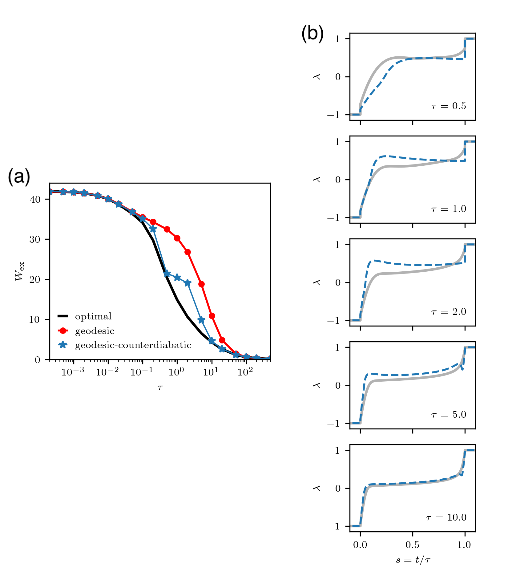
Figure S1: (a) Performance of optimal protocols from Zhong and DeWeese (2022) (black), geodesic (red dots), and geodesic-counterdiabatic protocols (blue stars), higher resolution reproduction of Fig.2(c) from main text. (b) Optimal protocols from Zhong and DeWeese (2022) (filled grey line) and geodesic-counterdiabatic protocols from Alg. 1 (broken blue line) for $\tau$ between $0.5$ to $10.0$, corresponding to the decrease in performance “peak” in (a). We see that for $\tau\sim 2$, the geodesic-counterdiabatic protocols overshoot the optimal protocols, corresponding to a reduction in performance.

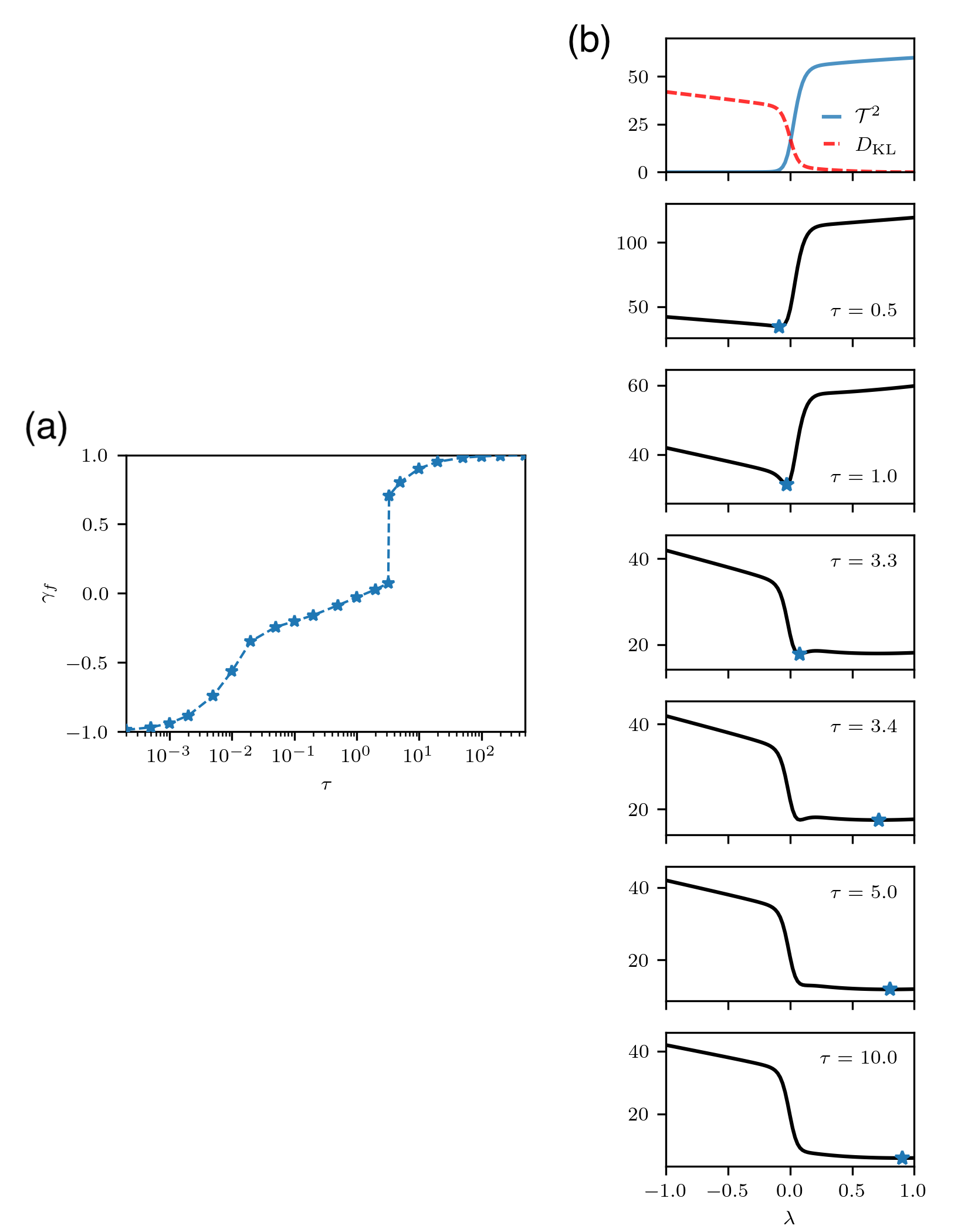
Figure S2: (a) The geodesic endpoint for geodesic-counterdiabatic protocols $\gamma_{f}=\arg\min_{\lambda}\ \mathcal{T}^{2}(\lambda_{i},\lambda)/\tau+D_{\mathrm{KL}}(\rho_{\lambda}^{\mathrm{eq}}|\rho_{f}^{\mathrm{eq}})$, as a function of protocol duration $\tau$. At $\tau\approx 3.3$ there is a discontinuity from $\gamma_{f}=0.073$ to $\gamma_{f}=0.706$. (b) The functions $\mathcal{T}^{2}(\lambda_{i},\lambda)$ (solid blue) and $D_{\mathrm{KL}}(\rho_{\lambda}^{\mathrm{eq}}|\rho_{f}^{\mathrm{eq}})$ (broken red), and their sum $\mathcal{T}^{2}(\lambda_{i},\lambda)/\tau+D_{\mathrm{KL}}(\rho_{\lambda}^{\mathrm{eq}}|\rho_{f}^{\mathrm{eq}})$ for various values of $\tau$. The blue star indicates the minimum, yielding $\gamma_{f}$, which suddenly jumps from $\gamma_{f}=0.073$ at $\tau=3.3$ to $\gamma_{f}=0.706$ at $\tau=3.4$, due to the existence of multiple local minima in the objective function.