Metallicity and $\alpha$-abundance for 48 million stars in low-extinction regions in the Milky Way

Abstract

We estimate ([M/H], [$\alpha$/M]) for 48 million giants and dwarfs in low dust extinction regions from the Gaia DR3 XP spectra by using tree-based machine-learning models trained on APOGEE DR17 and metal-poor star sample of Li et al. The root mean square error of our estimation is 0.0890 dex for [M/H] and 0.0436 dex for [$\alpha$/M], when we evaluate our models with the test data. Our estimation is most reliable for giants and metal-rich stars, because the training data are dominated by such stars. The high-[$\alpha$/M] stars and low-[$\alpha$/M] stars selected by our ([M/H], [$\alpha$/M]) show different kinematical properties for giants and low-temperature dwarfs. We further investigate how our machine-learning models extract information on ([M/H], [$\alpha$/M]). Intriguingly, our models seem to extract information on [$\alpha$/M] from Na D lines (589 nm) and Mg I line (516 nm). This result is understandable given the observed correlation between Na and Mg abundances in the literature. The catalog of ([M/H], [$\alpha$/M]) as well as their associated uncertainties will be publicly available online.

1 Introduction

1.1 Spectroscopic surveys and chemical abundances

The chemical abundances of stars imprint the chemistry of the gas from which they were formed. Determining the stellar chemical abundances is, therefore, an important task in understanding the history of the Milky Way. Many spectroscopic surveys conducted by ground-based telescopes (e.g., RAVE, Steinmetz et al. 2006; SEGUE, Yanny et al. 2009; APOGEE, Majewski et al. 2016; LAMOST, Zhao et al. 2012; GALAH, De Silva et al. 2015; Gaia-ESO, Gilmore et al. 2012) have obtained chemical abundances of millions of stars in the Milky Way and other local group galaxies based on the high-resolution ($\lambda/\Delta\lambda\gtrsim 20,000$) or low/medium-resolution ($\lambda/\Delta\lambda\simeq 2,000$–$20,000$) spectra taken from many years of observations.

1.2 Data mining of Gaia XP spectra

Recently, Gaia Data Release 3 (DR3) provided extremely low-resolution BP/RP spectra (hereafter XP spectra following the convention) with $\lambda/\Delta\lambda\sim 50$-$100$ for 219 million stars (De Angeli et al., 2022; Montegriffo et al., 2022; Gaia Collaboration et al., 2022). Although the XP spectra have much lower spectral resolution than the spectra of other spectroscopic surveys, the size and homogeneity of this data set has opened a new possibility to investigate the stellar atmospheric parameters (such as $T_{\rm eff}$, log g) and stellar chemical abundances (such as $\mathrm{[M/H]}$, $[\alpha/\mathrm{M}]$, [C/Fe], [N/Fe], [O/Fe]) for many stars by using machine learning (ML) models.

1.2.1 Before the publication of Gaia DR3

Before the launch of Gaia, Bailer-Jones (2010) explored a theoretical framework to infer the stellar atmospheric parameters, dust extinction, and metallicity [Fe/H] of stars with Gaia XP spectra. The author used synthetic spectra to test the method, but did not try to estimate $[\alpha/\mathrm{Fe}]$ from Gaia XP spectra.

When Gaia XP spectra were analyzed internally by the Gaia team, Gavel et al. (2021) used an ML algorithm called ExtraTrees to try to estimate $[\alpha/\mathrm{Fe}]$ from synthetic Gaia XP spectra and the actual, unpublished Gaia XP spectra. When they used a model which was trained on synthetic spectra, they were able to estimate $[\alpha/\mathrm{Fe}]$ of synthetic spectra, but were unable to estimate $[\alpha/\mathrm{Fe}]$ of Gaia XP spectra. When they used a model which was trained on the Gaia XP spectra, they were able to estimate $[\alpha/\mathrm{Fe}]$ from the Gaia XP spectra for cool stars ($\mbox{$T_{\rm eff}$}<5000\;\mathrm{K}$ or equivalently, $1.1<(G_{\mathrm{BP}}-G_{\mathrm{RP}})$), but were unable to estimate $[\alpha/\mathrm{Fe}]$ from Gaia XP-like synthetic spectra. Their finding indicates that estimating $[\alpha/\mathrm{Fe}]$ is difficult for stars with $5000\;\mathrm{K}<\mbox{$T_{\rm eff}$}$ or $(G_{\mathrm{BP}}-G_{\mathrm{RP}})<1.1$. Based on these findings, they inferred that their models appeared to estimate $[\alpha/\mathrm{Fe}]$ (of cool stars) by using indirect correlations between $[\alpha/\mathrm{Fe}]$ and other stellar properties including but not limited to the metallicity [Fe/H].

Witten et al. (2022) investigated the information content of the Gaia XP spectra and showed that the Gaia XP-like synthetic spectra of Solar-metallicity stars with $G=16$ do not have enough information to reliably estimate the $[\alpha/\mathrm{Fe}]$ abundance, unless $\mbox{$T_{\rm eff}$}<5000\;\mathrm{K}$ is satisfied, supporting the result in Gavel et al. (2021).

The results of Gavel et al. (2021) and Witten et al. (2022) indicate that extracting information on $[\alpha/\mathrm{M}]$ from Gaia XP spectra is challenging. However, we dare to tackle this problem in this paper due to the following reasons. First, the observed XP spectra used in Gavel et al. (2021) is not exactly the same as the XP spectra published in DR3. Second, Gavel et al. (2021) used only ExtraTrees algorithm. We note that other ML algorithms might be more suited to extract $[\alpha/\mathrm{M}]$ information. Third, Witten et al. (2022) pointed out the difficulty of estimating $[\alpha/\mathrm{Fe}]$ based on their analysis of synthetic spectra of stars with $G=16$ (see their Fig. 9), and it is unclear whether the same argument is valid for brighter stars. For example, their Fig. 3 indicated that the uncertainty in [Fe/H] for a star with $G=13$ is $\sim 4$ times smaller than that for a star with $G=16$. Thus, the uncertainty in $[\alpha/\mathrm{Fe}]$ of a $G=13$ star might be a few times smaller than that of a $G=16$ star. In such a case, trying to infer $[\alpha/\mathrm{Fe}]$ (or $[\alpha/\mathrm{M}]$) is still meaningful.

1.2.2 After the publication of Gaia DR3

After the publication of Gaia DR3, many authors have used the Gaia XP spectra to infer the stellar properties, including the chemical abundances (Rix et al., 2022; Andrae et al., 2023; Zhang et al., 2023; Bellazzini et al., 2023; Sanders & Matsunaga, 2023; Yao et al., 2024; Martin et al., 2023; Xylakis-Dornbusch et al., 2024).

Rix et al. (2022) did a pioneering work to estimate $(\mbox{$T_{\rm eff}$},\mbox{log~{}{\it g}},\mbox{$\mathrm{[M/H]}$})$ of 2 million giants within 30^∘ of the Galactic center. They used the reliable stellar parameters from APOGEE DR17 (Abdurro’uf et al., 2022) and trained the ML model called XGboost to infer the stellar parameters. Importantly, they used external catalog (AllWISE photometry; Cutri et al. 2021) to aid their model to infer the stellar parameters for stars with non-negligible dust extinction. Following the success of Rix et al. (2022), Andrae et al. (2023) estimated $(\mbox{$T_{\rm eff}$},\mbox{log~{}{\it g}},\mbox{$\mathrm{[M/H]}$})$ of 175 million stars across the sky. Their mean stellar parameter precision is 50 K in $T_{\rm eff}$, 0.08 dex in log g, and 0.1 dex in $\mathrm{[M/H]}$. In their work, they used a metal-poor star sample in Li et al. (2022) in addition to the APOGEE sample so that their training data cover a wide range of $\mathrm{[M/H]}$, which enhanced the reliability of $\mathrm{[M/H]}$ at the low-$\mathrm{[M/H]}$ region. Zhang et al. (2023) used a ML model based on a neural network to infer the stellar parameters $(\mbox{$T_{\rm eff}$},\mbox{log~{}{\it g}},\mbox{$\mathrm{[M/H]}$})$, parallax, and the dust extinction for 220 million stars with XP spectra. They used the LAMOST DR8 sample (Wang et al., 2022) as the training data, because it covers a wider parameter space than APOGEE sample. An interesting part of their model is that their model can predict the XP spectra given the input stellar parameters. More recently, Leung & Bovy (2023) used a modern ML models based on Transformer model (which is also used in Large Language Models) and showed a way to infer the stellar labels $(\mbox{$T_{\rm eff}$},\mbox{log~{}{\it g}},\mbox{$\mathrm{[M/H]}$})$ with high accuracy. Also, there is an attempt to produce a generative model of Gaia XP spectra (Laroche & Speagle, 2023), which may be useful to interpret the observed Gaia XP spectra directly, without estimating the stellar chemical abundances.

We note that some authors inferred the chemical abundances of stars from the XP spectra but did not publish the process as the main part of their paper (Belokurov et al., 2023; Chandra et al., 2023).

1.3 Scope of this paper: Estimation of $[\alpha/\mathrm{M}]$ from Gaia XP spectra

The previous works mentioned above have estimated $\mathrm{[M/H]}$ (or [Fe/H]), but none of them estimated $[\alpha/\mathrm{M}]$ (or [Mg/Fe]). This is partly because of the difficulty of estimating $[\alpha/\mathrm{M}]$, as presented by Gavel et al. (2021) and Witten et al. (2022). However, as mentioned earlier (Section 1.2.1) we dare to tackle this problem using a classical ML model that is different from the ExtraTrees model used in Gavel et al. (2021). The simpleness of our models enables us to investigate how the ML models infer the chemical abundances from the XP spectra.

While we were preparing our manuscript, we noticed that independent groups had tackled this problem with the same aim of estimating $[\alpha/\mathrm{M}]$ (Guiglion et al., 2024; Li et al., 2023). We note that these papers used a modern ML architecture, while we use a classical ML model, and thus the interpretation of the ML model is more straightforward in this paper. Guiglion et al. (2024) used the medium-resolution spectra from Gaia RVS (with $\lambda/\Delta\lambda\simeq 10,000$), in addition to the XP spectra. Also, Li et al. (2023) focused on giant stars, while we do not specifically restrict our analysis to giants.

1.4 Structure of this paper

Our primary goal in this paper is to estimate $\mathrm{[M/H]}$ and $[\alpha/\mathrm{M}]$ from Gaia XP spectra with classical ML models. This paper is organized as follows. In Section 2, we introduce the data set we used. In Section 3, we describe how we construct our ML models. In Section 4, we validated our estimation of $\mathrm{[M/H]}$ and $[\alpha/\mathrm{M}]$. In Section 5.1, we describe the catalog of ($\mathrm{[M/H]}$, $[\alpha/\mathrm{M}]$) derived from our analysis. In Section 6, we try to interpret how our ML models infer ($\mathrm{[M/H]}$, $[\alpha/\mathrm{M}]$), by quantifying which wavelength ranges of the XP spectra are important. In Section 7, we summarize this paper. In Appendix A and B, we present a detailed validation of or models.

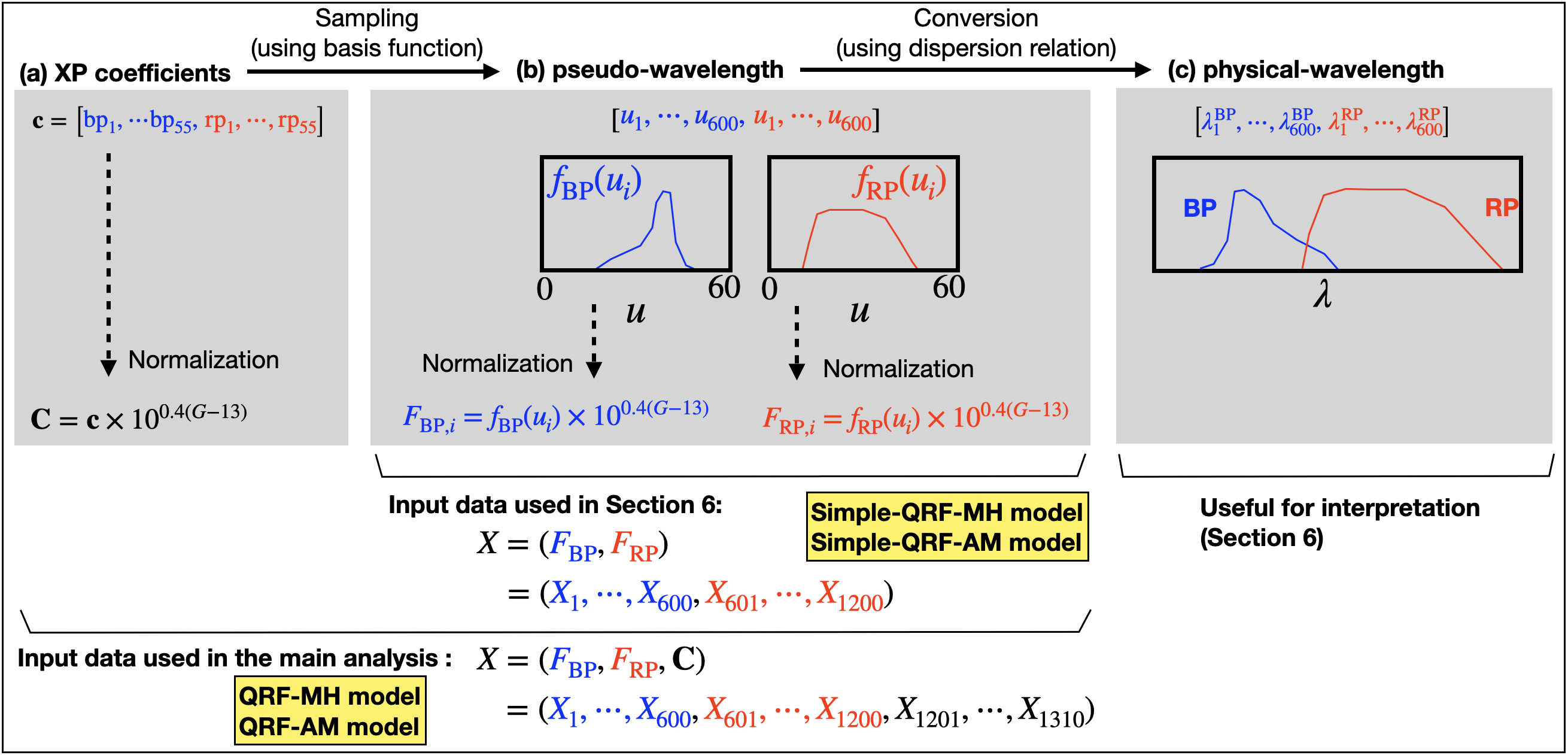
Figure 1: Schematic diagram of the data used in this paper.

2 Data

Here we describe the data sets used in this paper.

2.1 Sample stars with Gaia XP spectra

From Gaia DR3, we select 219 million stars for which the mean BP/RP spectrum (so-called XP spectrum) is available (has_xp_continuous=True in Gaia DR3). For each of these stars, Gaia provides 110 coefficients

$$\mbox{\boldmath$c$}=(bp_{1},\cdots,bp_{55},rp_{1},\cdots,rp_{55})$$ (1)

that represent the mean BP/RP spectra. Gaia also provides the uncertainty in $c$ and their correlations, but we neglect these quantities to simplify our analysis.

As shown in Figure 1, the coefficients $c$ can be converted into the mean BP and RP spectra $(f_{\mathrm{BP}},f_{\mathrm{RP}})$ in terms of the pseudo-wavelength $u$ (Montegriffo et al., 2022). Here, $0<u<60$ is a dimensionless quantity and it is differently defined for BP domain and RP domain. For example, $u=30$ defined in the BP domain and that in RP domain correspond to different wavelengths. By using $c$, we can express $f_{\mathrm{BP}}=f_{\mathrm{BP}}(u)$ and $f_{\mathrm{RP}}=f_{\mathrm{RP}}(u)$ for each star. In our analysis, we define equally-spaced 600 points $u_{i}=60\times(i-1)/599$, $(i=1,\cdots 600)$ within the range of $0\leq u\leq 60$. We evaluate $f_{\mathrm{BP}}(u_{i})$ and $f_{\mathrm{RP}}(u_{i})$, and save these 1200 quantities for each star.

In the main analysis of this paper, we use the 1310-dimensional information consisting of the 1200-dimensional flux data ($f_{\mathrm{BP}}(u_{i}),f_{\mathrm{RP}}(u_{i})$) and the 110-dimensional coefficients $c$.

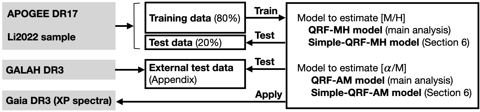
Figure 2: Summary of the data sets and models. We use the combined data from APOGEE DR17 and Li et al. (2022) to train and test our models (QRF-MH model to estimate $\mathrm{[M/H]}$, and QRF-AM model to estimate $[\alpha/\mathrm{M}]$). Because we have small number of dwarf stars in the training data, we additionally use GALAH DR3 data as the external data to test our models.

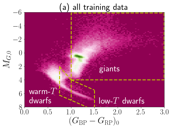
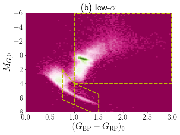
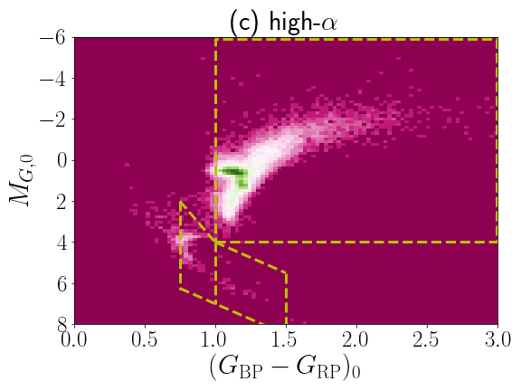
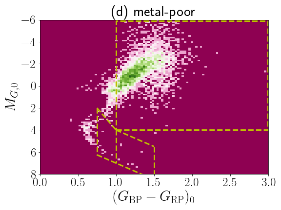
Figure 3: The distribution of stars in our training and test data in the photometric space.

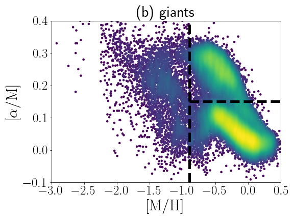
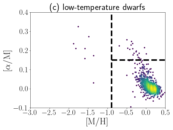
Figure 4: The distribution of stars in our training and test data in the chemical abundance space.

2.2 Training/test data

As shown in Fig. 2, we construct a data set of stars with known chemistry taken from either APOGEE DR17 data set (Abdurro’uf et al., 2022) or the data set in Li et al. (2022). We first introduce these data sets in Sections 2.2.1-2.2.2. Then we illustrate the properties of the combined catalog in Section 2.2.3.

2.2.1 APOGEE DR17

From APOGEE DR17 (Abdurro’uf et al., 2022), we select 115,249 stars from the value-added catalog (allStar-dr17-synspec_rev1.fits) that satisfy the following criteria: (i) Both $\mathrm{[M/H]}$ and $[\alpha/\mathrm{M}]$ are available; (ii) 0-6th, 8-10th, and 16-27th bits in the ASPCAPFLAG are zero; (iii) Third and fourth flags of STARFLAG are zero (avoiding objects with a very bright neighbor and objects with low signal-to-noise ratio); (iv) Fourth flag of EXTRATARG is zero (adopting the spectrum with the highest signal-to-noise ratio for stars with multiple observations); (v) Color excess $E(B-V)<0.1$ is satisfied (We multiply a scaling factor 0.86 to the color excess from the Schlegel et al. 1998 dust map, following Schlafly & Finkbeiner 2011.); (vi) Galactic latitude satisfies $|b|>5^{\circ}$; and (vii) XP spectra coefficients are available from Gaia DR3. The criteria (i)-(iv) are designed to select clean sample of APOGEE stars with reliable chemical abundances, while maintaining the sample size. The criteria (v) and (vi) aim to exclude stars whose XP spectra are significantly altered by the reddening (Bailer-Jones, 2010).

2.2.2 Metal-poor star catalog from Li et al. (2022)

Since there are few APOGEE stars with $\mbox{$\mathrm{[M/H]}$}\lesssim-2.5$, we also use the metal-poor stars in Li et al. (2022) in addition to the APOGEE stars (see Andrae et al. 2023). For brevity, we call this metal-poor sample as Li2022 sample. Among 385 stars in the Li2022 sample, we select 299 stars that satisfy the following criteria: (i) Both [Fe/H] and [Mg/Fe] are determined from Subaru observation; (ii) Color excess $E(B-V)<0.1$ is satisfied (adopting the value in Table 1 of Aoki et al. 2022, which is based on the 3D dust map of Green et al. 2018); (iii) XP spectra coefficients are available from Gaia DR3.

In the following analysis, we regard [Fe/H] as $\mathrm{[M/H]}$ and [Mg/Fe] as $[\alpha/\mathrm{M}]$, and merge the Li2022 sample to the APOGEE sample. We note that there is a star that is included in both APOGEE DR17 and Li2022, and we have confirmed for this star that its chemical abundances from these catalogs agree well with each other. For this duplicated star, we use the chemical abundances from Li et al. (2022) and discard the corresponding entry in the APOGEE catalog.

2.2.3 Combined data of APOGEE and Li2022 sample

The combined sample of APOGEE and Li2022 consists of 115,547 unique stars. The sample covers a wide range in metallicity ($-4.4\leq\mbox{$\mathrm{[M/H]}$}\leq+0.6$) and in $\alpha$-abundance ($-0.3\leq\mbox{$[\alpha/\mathrm{M}]$}\leq+1.1$). We randomly divide these stars into the training data set (80%) and the test data set (20%). The training data will be used in Section 3 to construct models to infer $(\mbox{$\mathrm{[M/H]}$},\mbox{$[\alpha/\mathrm{M}]$})$ from the XP spectra. The test data will be used to assess the performance of the models.

To understand the limitation of our models, it is important to understand the distribution of these stars in the color-magnitude diagram (CMD) and in the chemical space. As a basis for discussion, we photometrically define three types of stars (giants, low-temperature dwarfs, and warm-temperature dwarfs; see Fig. 3(a)). Also, we chemically define three groups of stars in the ($\mathrm{[M/H]}$, $[\alpha/\mathrm{M}]$)-space (low-$\alpha$, high-$\alpha$, and metal-poor stars (see Fig. 4(a)).

The stars in the training data are mostly giants and dwarfs (see Fig. 3(a)). In particular, giants are the dominant members of the training data independent of the stellar chemistry (see Fig. 3(b)-(d)). As seen in Fig. 4(c), most of the low/warm-temperature dwarfs in the training data belong to the low-$\alpha$ subsample (see Fig. 4(d)). Due to the paucity of the metal-poor dwarfs in the training data, we expect that it would be difficult for our models to infer ($\mathrm{[M/H]}$,$[\alpha/\mathrm{M}]$) of metal-poor dwarfs, which is confirmed in our later analysis.

2.3 External test data: GALAH DR3

To aid the test process of our models, we also prepare an external test data set taken from GALAH DR3. From GALAH DR3, we obtain the value-added catalog (GALAH_DR3_main_allstar_v2.fits; Buder et al. 2021). We extract stars that satisfy the following criteria: (i) Both [Fe/H] and $[\alpha/\mathrm{Fe}]$ are determined with high reliability (snr_c3_iraf>30, flag_sp=0, flag_fe_h=0, flag_alpha_fe=0); (ii) Color excess $E(B-V)<0.1$ is satisfied (adopting the procedure in Section 2.2.1); (iii) XP spectra coefficients are available from Gaia DR3. (iv) Stars are not included in the combined training/test data of APOGEE DR17 and Li2022.

This catalog contains 178,814 stars, including $\sim 8,000$ low-temperature dwarfs (with $\mbox{$T_{\rm eff}$}\lesssim 5000$ K). In contrast, the combined training/test data (from APOGEE DR17 and Li2022) only include $\sim 1000$ such dwarfs. Thus, this external test data are useful to test the performance of our models for low-temperature dwarfs.

3 Construction of the model

3.1 Quantile Regression Forests (QRF)

In this paper, we use an ML method named ‘Quantile Regression Forests (QRF)’ to infer ($\mathrm{[M/H]}$, $[\alpha/\mathrm{M}]$) from the XP spectra. The QRF is a non-parametric tree-based ensemble method, which is a generalized version of the Random Forest (RF) method. Since the QRF is not as widely used as the RF, we first describe the difference between RF and QRF.

Let us denote the input data as $X$ (in our case, the information of the XP spectra) and the target label to be estimated as $Y$ (in our case, $\mathrm{[M/H]}$ or $[\alpha/\mathrm{M}]$). In the RF, the algorithm uses multiple decision trees and tries to find the expected value of $Y$ given the data $X$, $E(Y\mid X)$. In the QRF, the algorithm also uses multiple decision trees, but it tries to find the probability distribution of $Y$ given the data $X$. Namely, for a given quantile $q$ in the range $0\leq q\leq 1$, the QRF estimates the value of $y$ such that the conditional probability $P(Y\leq y\mid X)=q$ is satisfied. In some implementations, the RF and QRF use the same set of decision trees. In such a case, while the QRF uses all the information of the decision trees to compute the probability distribution of $P(Y\mid X)$, the RF returns only the summary statistics of the decision trees $E(Y\mid X)$.

We adopt a publicly available QRF package quantile-forest (https://pypi.org/project/quantile-forest/). In this implementation, the QRF can estimate only a scalar target $Y$. Therefore, we construct a QRF model for $\mathrm{[M/H]}$ and $[\alpha/\mathrm{M}]$ separately. Namely, we only estimate $P(\mbox{$\mathrm{[M/H]}$}\mid X)$ and $P(\mbox{$[\alpha/\mathrm{M}]$}\mid X)$ for each star, and we do not estimate $P(\mbox{$\mathrm{[M/H]}$},\mbox{$[\alpha/\mathrm{M}]$}\mid X)$ for each star.

3.2 Input data for the QRF models

Since the XP coefficients are designed to represent the observed stellar flux as a function of the (psuedo-) wavelength, we first normalize the coefficients by multiplying a factor accounting for the apparent magnitude of the star. For each star, we use its $G$-band magnitude $G$ and compute (i) the normalized coefficient vector

$$\mbox{\boldmath$C$}=\mbox{\boldmath$c$}\times 10^{0.4(G-13)},$$ (2)

(ii) the normalized mean BP and RP spectra ($\mbox{\boldmath$F$}_{\mathrm{BP}}$ and $\mbox{\boldmath$F$}_{\mathrm{RP}}$), for which the $i$th element is given by

$$F_{\mathrm{BP},i} =f_{\mathrm{BP}}(u_{i})\times 10^{0.4(G-13)},$$ (3)

$$F_{\mathrm{RP},i} =f_{\mathrm{RP}}(u_{i})\times 10^{0.4(G-13)}.$$ (4)

In the main analysis of this paper, we use the 1310-dimensional vector

$$X=(\mbox{\boldmath$C$},\mbox{\boldmath$F$}_{\mathrm{BP}},\mbox{\boldmath$F$}_{\mathrm{RP}})$$ (5)

as the input of our QRF model. In Section 6, we use QRF models for which we only use 1200-dimensional information $X=(\mbox{\boldmath$F$}_{\mathrm{BP}},\mbox{\boldmath$F$}_{\mathrm{RP}})$ to enhance the interpretability of the model.

3.3 Training the QRF models

We train the QRF model by using the input vector $X$ and the target label $Y$ (either $\mathrm{[M/H]}$ or $[\alpha/\mathrm{M}]$) of the APOGEE and Li2022 samples. We use 80% of the data as the training data ($N_{\mathrm{train}}=92,437$ stars) and 20% of the data as the test data ($N_{\mathrm{test}}=23,110$ stars).

We set two hyperparameters, n_estimators=100 and max_features=0.5. The former hyperparameter, n_estimators, is the number of trees in the forest, and our choice of 100 is the default value. Our choice of the latter hyperparameter, max_features=0.5, is in between two widely adopted values of 0.333 (Hastie et al., 2001) and 1.0 (default value). When the QRF makes the decision tree, the algorithm keeps splitting the feature space (in our case, 1310-dimensional space of $X$). Our choice of max_features=0.5 means that the algorithm uses randomly selected 50% of the entire dimension (i.e., 655 dimensions) when looking for the best split. We have confirmed that the choice of the hyperparameters do not strongly affect the performance of the model. As explained in Section 3.1, we separately build a model for estimating $\mathrm{[M/H]}$ (hereafter QRF-MH model) and a model for estimating $[\alpha/\mathrm{M}]$ (hereafter QRF-AM model).

Since the QRF model can evaluate $P(Y\mid X)$, it can predict the label $Y$ for any specified percentile $q$. For brevity, we denote $y^{\mathrm{pred},q}_{k}$ as the $q$th percentile value of the predicted value of the label $Y$ for $k$th star. (For example, $y^{\mathrm{pred},50}_{k}$ corresponds to the predicted median value of the label $Y$ for $k$th star). Also, we denote $y_{k}^{\mathrm{spec}}$ to denote the spectroscopically determined (true) label for $k$th star. We separately train the QRF-MH and QRF-AM models such that the loss function

$$loss=\frac{1}{N_{\mathrm{train}}}\sum_{k\in\mathrm{Training\;data}}{\left(y^{\mathrm{pred},50}_{k}-y^{\mathrm{spec}}_{k}\right)}^{2}$$ (6)

is minimized.

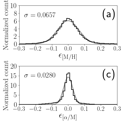
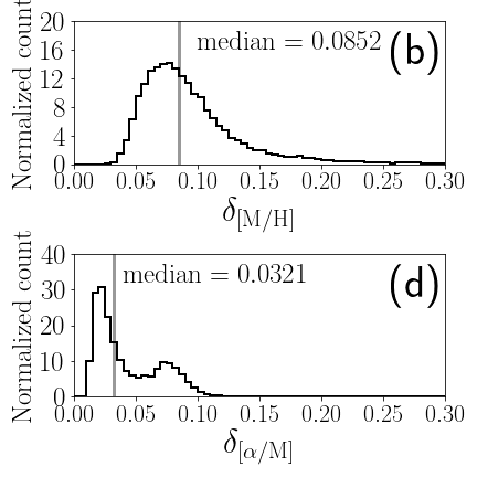
Figure 5: The performance of our models. (a) The histogram of $\epsilon_{\mathrm{[M/H]}}$. We also show a fitted Gaussian distribution and the standard deviation $\sigma$ (shown on the panel). (b) The histogram of $\delta_{\mathrm{[M/H]}}$, which has a single-peaked distribution with the median value shown on the panel. (c) The same as panel (a) but for the histogram of $\epsilon_{[\alpha/\mathrm{M}]}$. (d) The histogram of $\delta_{[\alpha/\mathrm{M}]}$, which has a double-peaked distribution with the median value shown on the panel.

4 Validation of the model using the test data

4.1 Root mean squared error

Once the QRF model is trained, we apply the model to the test data to measure the performance of the model. We define the root mean squared error (RMSE) for $\mathrm{[M/H]}$ and $[\alpha/\mathrm{M}]$ by

$$\mathrm{RMSE}=\sqrt{\frac{1}{N_{\mathrm{test}}}\sum_{k\in\mathrm{Test\;data}}{\left(y^{\mathrm{pred},50}_{k}-y^{\mathrm{spec}}_{k}\right)}^{2}}.$$ (7)

The results are summarized in Table 1. The overall performance of our models are represented by the RMSE values for the entire test data, which is 0.089 dex for $\mathrm{[M/H]}$ and 0.0436 dex for $[\alpha/\mathrm{M}]$. It is reassuring that these numbers are comparable to the corresponding numbers in the literature which used more modern ML architecture (e.g., Leung & Bovy 2023; Li et al. 2023). We note that we are only focusing on stars in low dust extinction regions with $E(B-V)<0.1$, while other authors also try to estimate the chemistry for stars with strong dust extinction (Rix et al., 2022; Andrae et al., 2023; Li et al., 2023).

We note that the performance of the models are most reliable for meal-rich stars with $\mbox{$\mathrm{[M/H]}$}>-1$, and the performance becomes worse at lower $\mathrm{[M/H]}$. However, even at $\mbox{$\mathrm{[M/H]}$}<-1$, the RMSE value for $[\alpha/\mathrm{M}]$ is as small as $0.0726$ dex, which is still useful to understand the distribution of stars in the ($\mathrm{[M/H]}$, $[\alpha/\mathrm{M}]$)-space.

We also divide our samples into giants and low/warm-temperature dwarfs and evaluate the RMSE values. We see that the performance for giants are most reliable, which is naturally understandable because our training data are dominated by giants.

We also evaluate the RMSE values by using the external test data taken from GALAH DR3. For the external test data, we see a similar trend to the results for the test data comprised of APOGEE and Li2022 sample.

4.2 Accuracy and precision for the entire test data

To further evaluate our models, we introduce two types of quantities. First, we introduce the difference $\epsilon$ between our predicted chemical abundance and the ‘true’ chemical abundance:

$$\epsilon_{\mathrm{[M/H]}} =\mbox{$\mathrm{[M/H]}$}^{\mathrm{pred},50}-\mbox{$\mathrm{[M/H]}$}^{\mathrm{spec}},$$ (8)

$$\epsilon_{[\alpha/\mathrm{M}]} =\mbox{$[\alpha/\mathrm{M}]$}^{\mathrm{pred},50}-\mbox{$[\alpha/\mathrm{M}]$}^{\mathrm{spec}},$$ (9)

for each star in the test data. The quantity $\epsilon$ satisfies $-\infty<\epsilon<\infty$, and it reflects the accuracy of our models.

Secondly, we introduce $\delta$ defined as

$$\delta_{\mathrm{[M/H]}} =\frac{1}{2}\left(\mbox{$\mathrm{[M/H]}$}^{\mathrm{pred},84}-\mbox{$\mathrm{[M/H]}$}^{\mathrm{pred},16}\right),$$ (10)

$$\delta_{[\alpha/\mathrm{M}]} =\frac{1}{2}\left(\mbox{$[\alpha/\mathrm{M}]$}^{\mathrm{pred},84}-\mbox{$[\alpha/\mathrm{M}]$}^{\mathrm{pred},16}\right),$$ (11)

for each star in the test data. The quantity $\delta$ satisfies $0\leq\delta$, and it reflects the precision of the labels for each star. We note that we can evaluate $\epsilon$ only for test data, while we can evaluate $\delta$ for any stars with XP spectra.

Table 1: Root mean squared error evaluated by applying our QRF-MH and QRF-AM models to the test data

Sample	RMSE	RMSE
	in $\mathrm{[M/H]}$	in $[\alpha/\mathrm{M}]$
Test data
Entire test data	0.0890	0.0436
Stars with [M/H]$>-1$	0.0768	0.0416
Stars with [M/H]$<-1$	0.220	0.0726
Giants	0.0767	0.0449
Giants with [M/H]$>-1$	0.0724	0.0441
Giants with [M/H]$<-1$	0.162	0.0652
Low-$T$ dwarfs	0.110	0.0332
Low-$T$ dwarfs with [M/H]$>-1$	0.0842	0.0332
Low-$T$ dwarfs with [M/H]$<-1$	1.14	0.0290
Warm-$T$ dwarfs	0.0784	0.0356
Warm-$T$ dwarfs with [M/H]$>-1$	0.0755	0.0354
Warm-$T$ dwarfs with [M/H]$<-1$	0.373	0.0790
External test data (GALAH)
Entire external test data	0.132	0.0817
Stars with [Fe/H]$>-1$	0.125	0.0781
Stars with [Fe/H]$<-1$	0.343	0.192
Giants	0.124	0.0777
Giants with [Fe/H]$>-1$	0.118	0.0754
Giants with [Fe/H]$<-1$	0.230	0.126
Low-$T$ dwarfs	0.174	0.0795
Low-$T$ dwarfs with [Fe/H]$>-1$	0.168	0.0780
Low-$T$ dwarfs with [Fe/H]$<-1$	0.924	0.330
Warm-$T$ dwarfs	0.133	0.0812
Warm-$T$ dwarfs with [Fe/H]$>-1$	0.129	0.0798
Warm-$T$ dwarfs with [Fe/H]$<-1$	0.602	0.280

Note. — Giants and dwarfs are selected from the test data in the same manner as in Fig. 3 (see footnote 2).

4.2.1 Accuracy and precision for the entire test data

Figs. 5(a) and 5(c) show the histogram of $\epsilon_{\mathrm{[M/H]}}$ and $\epsilon_{[\alpha/\mathrm{M}]}$ for the entire test data. The distributions of $\epsilon_{\mathrm{[M/H]}}$ or $\epsilon_{[\alpha/\mathrm{M}]}$ are almost symmetric around zero, which indicates that there is no obvious systematic error in inferring ($\mathrm{[M/H]}$,$[\alpha/\mathrm{M}]$) in our models. The distributions of $\epsilon_{\mathrm{[M/H]}}$ or $\epsilon_{[\alpha/\mathrm{M}]}$ can be approximated by Gaussian distributions, with standard deviations $\sigma=0.0657$ and $0.0282$, respectively. These numbers are 30%–40% smaller than the corresponding RMSE values in Table. 1, which indicates that the histograms in Figs. 5(a) and 5(c) have a fatter tail than a Gaussian distribution.

Figs. 5(b) and 5(d) show the histogram of $\delta_{\mathrm{[M/H]}}$ and $\delta_{[\alpha/\mathrm{M}]}$ for the entire test data. We note that the typical precision of our models can be inferred from the median of the distribution of $\delta_{\mathrm{[M/H]}}$ or $\delta_{[\alpha/\mathrm{M}]}$. The median value of $\delta_{\mathrm{[M/H]}}$ ($=0.0852$ dex) is roughly consistent with the RMSE (0.0890 dex) of our model for $\mathrm{[M/H]}$. Interestingly, the histogram of $\delta_{[\alpha/\mathrm{M}]}$ has two peaks, at 0.02 dex (first peak) and at 0.07 dex (secondary peak). As we will see in Fig. 7(a), the first peak corresponds to a case when high-$\alpha$ (or low-$\alpha$) stars are correctly assigned high (or low) $\alpha$ abundances, while the second peak corresponds to a case in which high-$\alpha$ (or low-$\alpha$) stars are incorrectly assigned low (or high) $\alpha$ abundances.

So far, we have investigated the performance of our models based on four quantities, $(\mbox{$\epsilon_{\mathrm{[M/H]}}$},\mbox{$\epsilon_{[\alpha/\mathrm{M}]}$}$, $\mbox{$\delta_{\mathrm{[M/H]}}$},\mbox{$\delta_{[\alpha/\mathrm{M}]}$})$. In Appendix A, we evaluate how the performance depends on the chemical abundance $(\mbox{$\mathrm{[M/H]}$},\mbox{$[\alpha/\mathrm{M}]$})$, the apparent magnitude $G$, the absolute magnitude $M_{G,0}$ (i.e., evolutionary stage of the star) and the color excess $E(B-V)$.

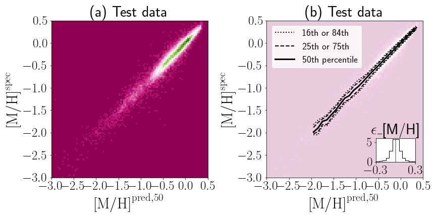
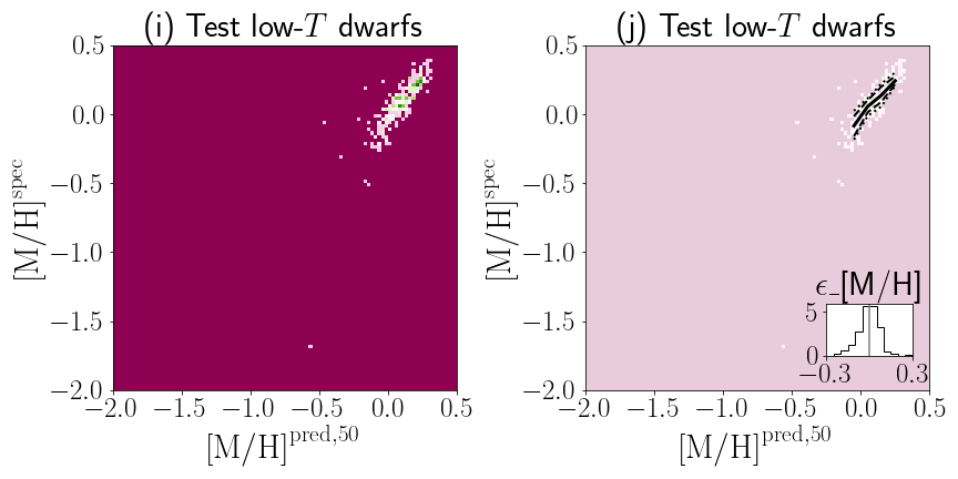
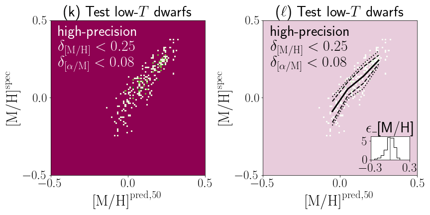
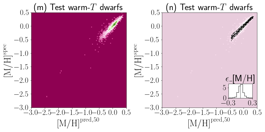
Figure 6: The performance of the QRF-MH model (our model for estimating $\mathrm{[M/H]}$) applied to the test data. In all panels, we show the predicted abundance (horizontal axis) and spectroscopic abundance (vertical axis). From the top to bottom rows, we show the distribution of stars in the entire test data (top row), giants in the test data (second row), low-temperature dwarfs in the test data (third row), and warm-temperature dwarfs in the test data (bottom row). The first column from the left displays the density distribution. The second column shows the (2.5th, 16th, 50th, 84th, 97.5th) percentile values of the spectroscopic abundance as a function of the predicted abundance. We also show the normalized histogram of the deviation of our predicted abundance relative to the spectroscopic abundance $(\mbox{$\epsilon_{\mathrm{[M/H]}}$}=\mbox{$\mathrm{[M/H]}$}^{\mathrm{pred,50}}-\mbox{$\mathrm{[M/H]}$}^{\mathrm{spec}})$. The third and fourth columns are the same as the first and second columns, respectively, but selecting only high-precision subsample with $\mbox{$\delta_{\mathrm{[M/H]}}$}<0.25$ and $\mbox{$\delta_{[\alpha/\mathrm{M}]}$}<0.08$. In some panels, the ranges of the horizontal and vertical axes are different from other panels for clarity.

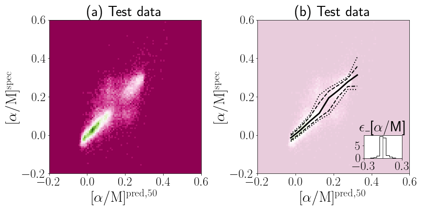
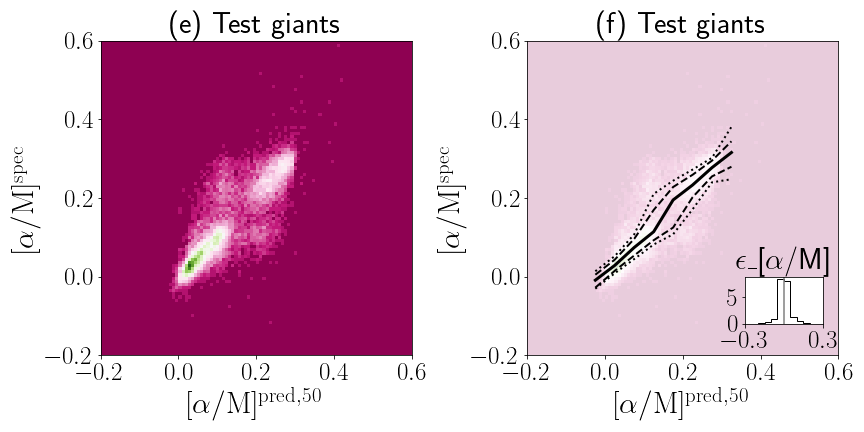
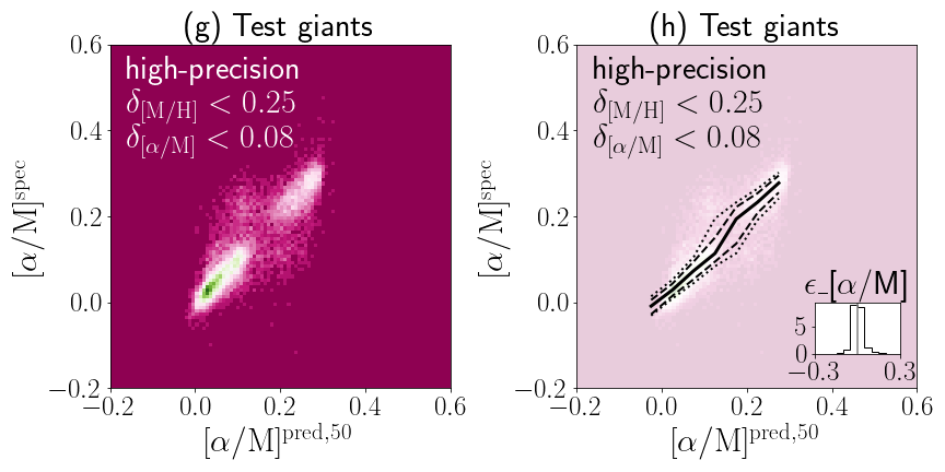
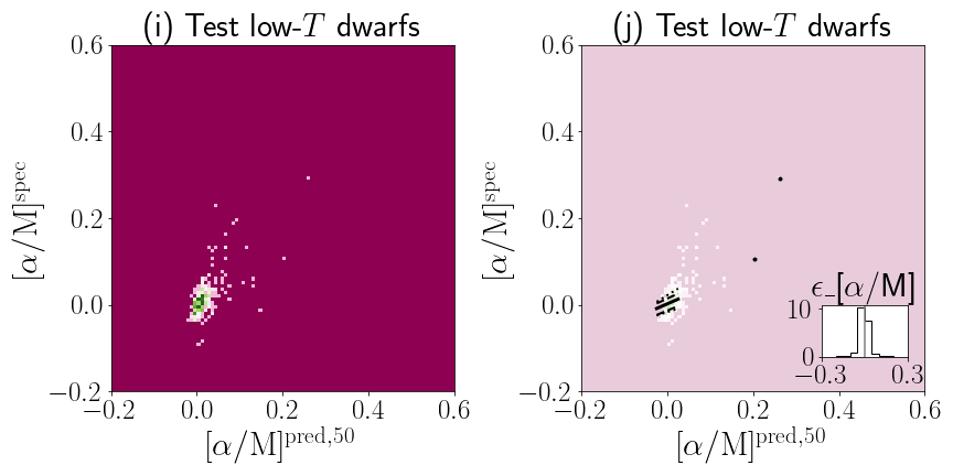
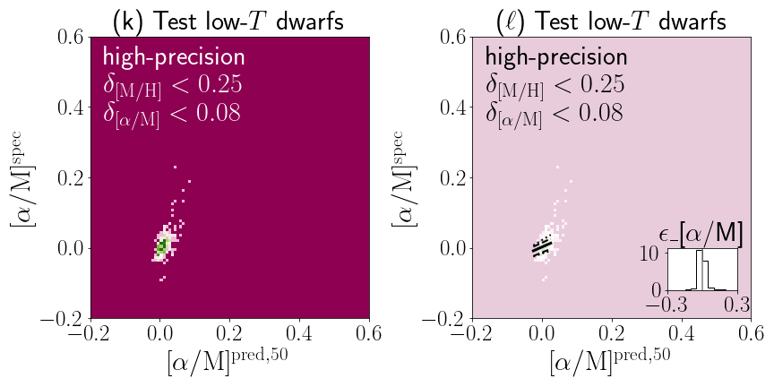
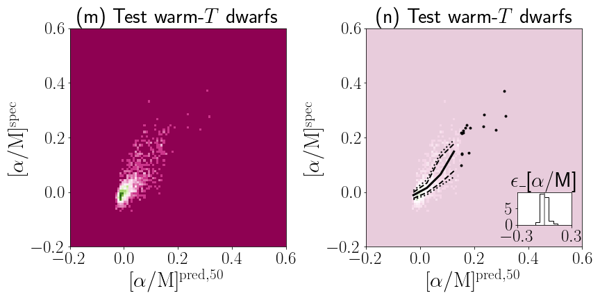
Figure 7: The same as Fig. 6, but showing the detailed performance of the QRF-AM model (our model for estimating $[\alpha/\mathrm{M}]$) applied to the test data. On panel (n), we plot the stars with $\mbox{$[\alpha/\mathrm{M}]$}^{\mathrm{pred,50}}>0.15$ with black dots to highlight that the majority of them are genuine high-$\alpha$ stars ($\mbox{$[\alpha/\mathrm{M}]$}^{\mathrm{spec}}>0.15$).

4.2.2 Accuracy of $\mathrm{[M/H]}$ for giants and dwarfs

Fig. 6 presents the distribution of stars in the test data in the $(\mbox{$\mathrm{[M/H]}$}^{\mathrm{pred,50}},\mbox{$\mathrm{[M/H]}$}^{\mathrm{spec}})$-space. (We note that Fig. 25 is the same as Fig. 6, but using the external test data from GALAH DR3.) In Fig. 6, the top row corresponds to the results for the entire test data. The second, third, and fourth rows correspond to the different photometric selection of stars.

(1) Giants

The second row of Fig. 6 shows the performance of our model to estimate $\mathrm{[M/H]}$, by using the giants in the test data. (Because the test data are dominated by giants, the second row looks similar to the top row.)

We see from the clear diagonal distribution in Fig. 6(e) that our QRF-MH model can nicely predict $\mathrm{[M/H]}$ at $-3\lesssim\mbox{$\mathrm{[M/H]}$}$. Fig. 6(f) shows the same distribution, but oveplotting the percentile values of $\mbox{$\mathrm{[M/H]}$}^{\mathrm{spec}}$ as a function of $\mbox{$\mathrm{[M/H]}$}^{\mathrm{pred,50}}$. The tight alignment of these percentile value profiles indicates the high precision in predicting $\mathrm{[M/H]}$ in our model. The inset in Fig. 6(f) shows the histogram of $\epsilon_{\mathrm{[M/H]}}$. The symmetric distribution of this histogram centered around $\mbox{$\epsilon_{\mathrm{[M/H]}}$}\sim 0$ indicates that there is no obvious systematic error in $\mathrm{[M/H]}$ for giants in the test data.

One of the advantages of our models is that we can evaluate the uncertainties $\delta_{\mathrm{[M/H]}}$ and $\delta_{[\alpha/\mathrm{M}]}$ in our prediction of the labels. By requiring $\mbox{$\delta_{\mathrm{[M/H]}}$}<0.25$ and $\mbox{$\delta_{[\alpha/\mathrm{M}]}$}<0.08$, we define a high-precision subsample of the stars and displayed the results in Figs. 6(g) and (h). We do not see a drastic change from Fig. 6(e) to Fig. 6(g), because a large fraction of giants satisfy these criteria (see Fig. 5(b) for a reference).

(2) Low-temperature dwarfs

The third row in Fig. 6 is the same as the second row, but using low-temperature dwarfs. Although our test data contain only 257 low-temperature dwarfs (240 of them are high-precision), we can recognize the diagonal feature in panels (i) and (k). The histograms of $\epsilon_{\mathrm{[M/H]}}$ has a slightly fatter tail at $\mbox{$\epsilon_{\mathrm{[M/H]}}$}<0$ than at $\mbox{$\epsilon_{\mathrm{[M/H]}}$}>0$, but the estimation of $\mathrm{[M/H]}$ is probably acceptable for low-temperature dwarfs, as long as $\mbox{$\mathrm{[M/H]}$}\gtrsim-0.1$.

The above-mentioned results are supported by the external test data from GALAH DR3, which contains a larger number of low-temperature dwarfs (see the third row of Fig. 25 in Appendix B). In particular, there is an almost-linear trend between $\mbox{$\mathrm{[M/H]}$}^{\mathrm{pred,50}}$ and $\mathrm{[Fe/H]}^{\mathrm{spec}}_{\mathrm{GALAH}}$ at $-0.3\lesssim\mbox{$\mathrm{[M/H]}$}^{\mathrm{pred,50}}$.

(3) Warm-temperature dwarfs

The bottom row in Fig. 6 is the same as the second row, but using warm-temperature dwarfs. We have 1518 low-temperature dwarfs (of which 1470 are high-precision), and we recognize a diagonal feature in panels (m) and (o) at $-0.5\lesssim\mbox{$\mathrm{[M/H]}$}^{\mathrm{pred,50}}$. The histograms of $\epsilon_{\mathrm{[M/H]}}$ look symmetric, suggesting negligible systematic error in estimating $\mathrm{[M/H]}$ for warm-temperature dwarfs.

The above-mentioned results are confirmed by the external test data from GALAH DR3 (see the bottom row of Fig. 25).

4.2.3 Accuracy of $[\alpha/\mathrm{M}]$ for giants and dwarfs

Fig. 7 presents the distribution of stars in the test data in the $(\mbox{$[\alpha/\mathrm{M}]$}^{\mathrm{pred,50}},\mbox{$[\alpha/\mathrm{M}]$}^{\mathrm{spec}})$-space. (We note that Fig. 26 is the same as Fig. 7, but using the GALAH data.) Again, the top row of Fig. 7 corresponds to the results for the entire test data. The other rows correspond to the different photometric selection of stars.

(1) Giants

The second row in Fig. 7 shows the performance of our model for giants. In Fig. 7(e), the majority of stars are distributed almost diagonally, suggesting that our QRF-AM model can estimate realistic $[\alpha/\mathrm{M}]$ for most of the giants in the test data. There are some stars with off-diagonal distribution in Fig. 7(e). Some of these stars are recognized by our model as low-$\alpha$ stars but actually high-$\alpha$ stars, and vice versa. The fraction of such stars is reduced if we select the high-precision subset of stars, as shown in panels (g) and (h). The symmetric shape of the histograms of $\epsilon_{[\alpha/\mathrm{M}]}$ suggests that we have no obvious systematic error in $[\alpha/\mathrm{M}]$ for giants.

(2) Low-temperature dwarfs

The third row in Fig. 7 is the same as the second row, but using low-temperature dwarfs. In panels (j) and ($\ell$), we see a marginal, positive correlation between $\mbox{$[\alpha/\mathrm{M}]$}^{\mathrm{pred,50}}$ and $\mbox{$[\alpha/\mathrm{M}]$}^{\mathrm{spec}}$. In Fig. 7(j), we have two low-temperature dwarfs with $\mbox{$[\alpha/\mathrm{M}]$}^{\mathrm{pred,50}}>0.15$ (shown by black dots). Among these two stars, one star (50 %) actually have $\mbox{$[\alpha/\mathrm{M}]$}^{\mathrm{spec}}_{\mathrm{GALAH}}>0.15$. However, due to the limited number of low-temperature dwarfs in the test data, the trend is not clear.

In this regard, it is worth mentioning the performance of our QRF-AM model for the external test data from GALAH (see the third row of Fig. 26). Notably, as seen in Fig. 26(j), there is a positive correlation between $\mbox{$[\alpha/\mathrm{M}]$}^{\mathrm{pred,50}}$ and $\mbox{$[\alpha/\mathrm{Fe}]$}^{\mathrm{spec}}_{\mathrm{GALAH}}$ at $0\lesssim\mbox{$[\alpha/\mathrm{M}]$}^{\mathrm{pred,50}}\lesssim 0.3$. In Fig. 26($\ell$), we have 55 low-temperature dwarfs with $\mbox{$[\alpha/\mathrm{M}]$}^{\mathrm{pred,50}}>0.15$ (shown by black dots). Among these 55 stars, 41 stars (75 %) actually have $\mbox{$[\alpha/\mathrm{M}]$}^{\mathrm{spec}}_{\mathrm{GALAH}}>0.15$. (In Fig. 26(j), this fraction is $38\%=(432/1151)$, which is reduced because the sample also includes low-precision stars.) From this exercise, we see that our QRF-AM model extract some information on $[\alpha/\mathrm{M}]$ from the XP spectra for low-temperature dwarfs, especially for high-precision sample.

(3) Warm-temperature dwarfs

The bottom row in Fig. 7 is the same as the second row, but using warm-temperature dwarfs. In panels (n) and (p), we recognize a clear positive trend between $\mbox{$[\alpha/\mathrm{M}]$}^{\mathrm{pred,50}}$ and $\mbox{$[\alpha/\mathrm{M}]$}^{\mathrm{spec}}$ at $-0.05<\mbox{$[\alpha/\mathrm{M}]$}^{\mathrm{pred,50}}<0.2$ although the number of stars with high-$\mbox{$[\alpha/\mathrm{M}]$}^{\mathrm{pred,50}}$ is limited.

In Fig. 7(p), we have 7 warm-temperature dwarfs with $\mbox{$[\alpha/\mathrm{M}]$}^{\mathrm{pred,50}}>0.15$ (shown by black dots). Among these 7 stars, 5 stars (71 %) actually have $\mbox{$[\alpha/\mathrm{M}]$}^{\mathrm{spec}}>0.15$. In Fig. 7(n), this fraction is $75\%(=12/16)$, which is surprisingly good given that the sample also include low-precision stars. (As a reference, in Fig. 26(n) and Fig. 26(p), this fraction is $75\%(=696/932)$ and $87\%(=34/39)$, respectively.) From this exercise, we see that our QRF-AM model extract some information on $[\alpha/\mathrm{M}]$ from the XP spectra for warm-temperature dwarfs. However, as we will discuss in Section 5.3 (see Fig. 15), we are not very comfortable with our estimates of ($\mathrm{[M/H]}$, $[\alpha/\mathrm{M}]$) due to an independent analysis on the chemo-dynamical correlation of the warm-temperature dwarfs.

Table 2: Description of the output data

Quantity	Description
source_id	source_id in Gaia DR3
phot_g_mean_mag	$G$-band magnitude (Gaia DR3)
phot_bp_mean_mag	$G_{\mathrm{BP}}$-band magnitude (Gaia DR3)
phot_rp_mean_mag	$G_{\mathrm{RP}}$-band magnitude (Gaia DR3)
l	Galactic longitude (Gaia DR3)
b	Galactic latitude (Gaia DR3)
ra	Right ascension (Gaia DR3)
dec	Declination (Gaia DR3)
parallax	Parallax without zero-point correction (Gaia DR3)
parallax_error	Parallax error (Gaia DR3)
ebv_dustmaps_086	$E(B-V)$ estimated from Schlegel et al. (1998) dust map multiplied by a factor 0.86
bool_in_training_sample	Boolean data indicating whether the star is included in the training data
bool_flag_cmd_good	Boolean data indicating whether the star satisfies the simple CMD cut indicated in Fig. 8
mh_2p5_qrf	2.5th percentile value of $\mathrm{[M/H]}$ estimated from our QRF model
mh_10_qrf	10th percentile value of $\mathrm{[M/H]}$ estimated from our QRF model
mh_16_qrf	16th percentile value of $\mathrm{[M/H]}$ estimated from our QRF model
mh_25_qrf	25th percentile value of $\mathrm{[M/H]}$ estimated from our QRF model
mh_50_qrf	50th percentile value of $\mathrm{[M/H]}$ estimated from our QRF model
mh_75_qrf	75th percentile value of $\mathrm{[M/H]}$ estimated from our QRF model
mh_84_qrf	84th percentile value of $\mathrm{[M/H]}$ estimated from our QRF model
mh_90_qrf	90th percentile value of $\mathrm{[M/H]}$ estimated from our QRF model
mh_97p5_qrf	97.5th percentile value of $\mathrm{[M/H]}$ estimated from our QRF model
alpham_2p5_qrf	2.5th percentile value of $[\alpha/\mathrm{M}]$ estimated from our QRF model
alpham_10_qrf	10th percentile value of $[\alpha/\mathrm{M}]$ estimated from our QRF model
alpham_16_qrf	16th percentile value of $[\alpha/\mathrm{M}]$ estimated from our QRF model
alpham_25_qrf	25th percentile value of $[\alpha/\mathrm{M}]$ estimated from our QRF model
alpham_50_qrf	50th percentile value of $[\alpha/\mathrm{M}]$ estimated from our QRF model
alpham_75_qrf	75th percentile value of $[\alpha/\mathrm{M}]$ estimated from our QRF model
alpham_84_qrf	84th percentile value of $[\alpha/\mathrm{M}]$ estimated from our QRF model
alpham_90_qrf	90th percentile value of $[\alpha/\mathrm{M}]$ estimated from our QRF model
alpham_97p5_qrf	97.5th percentile value of $[\alpha/\mathrm{M}]$ estimated from our QRF model

5 Results

5.1 The catalog of $\mathrm{[M/H]}$ and $[\alpha/\mathrm{M}]$

After training the QRF-MH and QRF-AM models, we first apply our models for the entire catalog of stars with Gaia XP spectra (219 million stars). Among these stars, we publish the labels for 48 million stars with $E(B-V)<0.1$ at the Zenodo database (https://zenodo.org/records/10902172). We describe the columns of the published catalog in Table 2.

Fig. 8 shows the CMD of our published catalog. We see that some fraction of stars in the catalog are hot dwarfs and white dwarfs, which are not represented by our training data (see also Fig. 3). The users of the catalog need to avoid these stars. As a simple way to omit these stars, we select stars that satisfy

$$0.3 <(G_{\mathrm{BP}}-G_{\mathrm{RP}})_{0}<2.2$$ (12)

$$M_{G,0} <3\times(G_{\mathrm{BP}}-G_{\mathrm{RP}})_{0}+5,$$ (13)

and flag these stars as bool_flag_cmd_good=True in our catalog. The corresponding region is shown by the white solid line in Fig. 8. Among 48 million stars with $E(B-V)<0.1$, about 46 million stars satisfy this simple CMD cut. This flag should be used to avoid stars with unreliable estimates of the chemistry. However, we do not attempt to state that all the stars with bool_flag_cmd_good=True have reliable estimates of their chemistry. The reliability of the estimated values of ($\mathrm{[M/H]}$, $[\alpha/\mathrm{M}]$) should be carefully analyzed by using other information, such as the stellar evolutionary stage (e.g., giants or dwarfs), parallax, $\delta_{\mathrm{[M/H]}}$ or $\delta_{[\alpha/\mathrm{M}]}$.

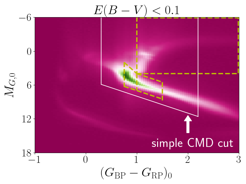
Figure 8: CMD of the stars in our catalog. The region above the white solid line satisfies bool_flag_cmd_good=True, which roughly corresponds to the region covered by our training data. The regions surrounded by yellow dashed lines are the same as in Fig. 3. We note that the stars in the catalog satisfies $E(B-V)<0.1$.

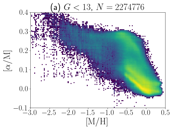
Figure 9: The distribution of low-extinction stars ($E(B-V)<0.1$) in our catalog with different $G$-band magnitude ranges. (a) Stars with $13<G$. (b) Stars with $13<G<14$. (c) Stars with $14<G<15$. (d) Stars with $15<G$. We have excluded stars in the training data.

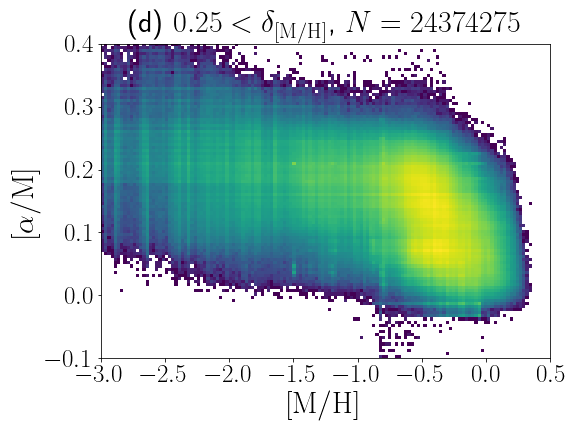
Figure 10: The distribution of low-extinction stars ($E(B-V)<0.1$) in our catalog with different $\delta_{\mathrm{[M/H]}}$ ranges. (a) Stars with $\mbox{$\delta_{\mathrm{[M/H]}}$}<0.1$. (b) Stars with $0.1<\mbox{$\delta_{\mathrm{[M/H]}}$}<0.2$. (c) Stars with $0.2<\mbox{$\delta_{\mathrm{[M/H]}}$}<0.25$. (d) Stars with $0.25<\mbox{$\delta_{\mathrm{[M/H]}}$}$. We have excluded stars in the training data.

Figure 11: The distribution of low-extinction stars ($E(B-V)<0.1$) in our catalog with different $\delta_{[\alpha/\mathrm{M}]}$ ranges. (a) Stars with $\mbox{$\delta_{[\alpha/\mathrm{M}]}$}<0.08$. (b) Stars with $0.08<\mbox{$\delta_{[\alpha/\mathrm{M}]}$}<0.1$. (c) Stars with $0.1<\mbox{$\delta_{[\alpha/\mathrm{M}]}$}<0.2$. (d) Stars with $0.2<\mbox{$\delta_{[\alpha/\mathrm{M}]}$}$. We have excluded stars in the training data.

Figure 12: The distribution of stars in the $(\mbox{$\mathrm{[M/H]}$},\mbox{$[\alpha/\mathrm{M}]$})$-space estimated from our models. In all of the plots, we show Solar-neighbor stars ($7\,\mathrm{kpc}<R<9\,\mathrm{kpc}$, $|z|<3\,\mathrm{kpc}$) with low dust extinction ($E(B-V)<0.1$) and good parallax measurements (fractional parallax error smaller than 20%). We also note that we have excluded stars in the training data. (a) Stars without further cuts. (b) Giant stars. (c) Low-temperature main-sequence stars. (d) Warm-temperature main-sequence stars. Panels (e), (f), (g), and (h) are the same as panels (a), (b), (c), and (d), respectively, but with further constraints of $\mbox{$\delta_{\mathrm{[M/H]}}$}<0.2$ and $\mbox{$\delta_{[\alpha/\mathrm{M}]}$}<0.07$. Only a portion of the data are shown for clarity, as described in the lower left corner of each panel.

5.2 Chemical distribution of stars

Here we investigate the distribution of stars with Gaia XP spectra in the chemistry space. In Sections 5.2.1-5.2.2, we restrict ourselves to low-extinction stars ($E(B-V)<0.1$) that are not in the training data. In Section 5.2.3, we further restrict ourselves to stars that are in the Solar cylinder ($7<R/\,\mathrm{kpc}<9$, $|z|<3\,\mathrm{kpc}$) and have good parallax measurements (parallax_over_error>5 in Gaia DR3).

In the following, when we refer to our estimated values of $\mathrm{[M/H]}$ or $[\alpha/\mathrm{M}]$, we simply use $\mbox{$\mathrm{[M/H]}$}=\mbox{$\mathrm{[M/H]}$}^{\mathrm{pred,50}}$ or $\mbox{$[\alpha/\mathrm{M}]$}=\mbox{$[\alpha/\mathrm{M}]$}^{\mathrm{pred,50}}$ for brevity.

5.2.1 Dependence on $G$

Fig. 9 shows the $(\mbox{$\mathrm{[M/H]}$},\mbox{$[\alpha/\mathrm{M}]$})$-distribution for different ranges of $G$. We see a clear bimodality of low-$\alpha$ and high-$\alpha$ sequences at $G<13$ (Fig. 9(a)), and the bimodality is marginally recognized at $13<G<15$ (Figs. 9(b) and 9(c)). In contrast, we do not see the bimodal structure at $15<G$. This result indicates that our estimates of $\mathrm{[M/H]}$ and $[\alpha/\mathrm{M}]$ are reasonable for bright stars and deteriorate with increasing $G$. We confirm this view in Appendix A (see Fig. 21), where we directly check the validity of our estimates by using the test data with different $G$-band magnitude. Our finding of the difficulty in estimating $\mathrm{[M/H]}$ or $[\alpha/\mathrm{M}]$ for faint stars is consistent with Witten et al. (2022).

5.2.2 Dependence on $\delta_{\mathrm{[M/H]}}$ and $\delta_{[\alpha/\mathrm{M}]}$

Figs. 10 and 11 show the chemical distribution of stars for different ranges of the precision of our estimates ($\delta_{\mathrm{[M/H]}}$ and $\delta_{[\alpha/\mathrm{M}]}$). We see a bimodality of low-$\alpha$ and high-$\alpha$ sequences for stars with $\mbox{$\delta_{\mathrm{[M/H]}}$}<0.1$ (Fig. 10(a)) and for stars with $\mbox{$\delta_{[\alpha/\mathrm{M}]}$}<0.08$ (Fig. 11(a)), but the bimodality is not as clearly seen for stars with other ranges of $\delta_{\mathrm{[M/H]}}$ or $\delta_{[\alpha/\mathrm{M}]}$. This result indicates that the values of $\delta_{\mathrm{[M/H]}}$ and $\delta_{[\alpha/\mathrm{M}]}$ can be used to select stars for which we have reliable estimates of $\mathrm{[M/H]}$ or $[\alpha/\mathrm{M}]$.

5.2.3 Dependence on the stellar evolutionary stage

In Fig. 12, we investigate the chemical distribution of stars with different evolutionary stages. After selecting Solar-neighbor stars with good parallax measurements (see the first paragraph of Section 5.2) we select giants, low/warm-temperature dwarfs based on the location in the CMD in the same manner as in Section 2.2.3 (see footnote 2).

We note that Witten et al. (2022) pointed out that estimating $[\alpha/\mathrm{M}]$ is difficult (for faint stars with $G=16$) at $\mbox{$T_{\rm eff}$}>5000$ K, which roughly corresponds to $(G_{\mathrm{BP}}-G_{\mathrm{RP}})_{0}\lesssim 1.1$ (see also Gavel et al. 2021). The warm-temperature main-sequence stars (with $(G_{\mathrm{BP}}-G_{\mathrm{RP}})_{0}<1$) are selected to investigate this issue.

Panels (a)-(d) in Fig. 12 show the chemical distribution of stars without any CMD selections (panel (a)), of giants (panel (b)), of low-temperature dwarfs (panel (c)), and of warm-temperature dwarfs (panel (d)). Panels (e)-(h) are the same as panels (a)-(d), respectively, but with further constraints of $\mbox{$\delta_{\mathrm{[M/H]}}$}<0.25$ and $\mbox{$\delta_{[\alpha/\mathrm{M}]}$}<0.08$ (i.e., high-precision subsample).

It is intriguing to note that the clear bimodality in the ($\mathrm{[M/H]}$, $[\alpha/\mathrm{M}]$)-space is visible for giants, even before applying the high-precision selection. This result indicates that our estimates of ($\mathrm{[M/H]}$, $[\alpha/\mathrm{M}]$) for giants have higher reliability than dwarfs. We also note that the fraction of stars with high-precision estimates of ($\mathrm{[M/H]}$, $[\alpha/\mathrm{M}]$) is as high as $\sim$68% for giants. (As shown in Fig. 12, we have 1,054,004 and 710,744 giants in panels (b) and (f), respectively.)

For warm- and low-temperature dwarfs, we do not see the clear bimodality in panels (c) or (d), but the bimodality can be seen in their high-precision subsample (in panels (g) and (h)). These results indicate that most stars with $\mbox{$[\alpha/\mathrm{M}]$}>0.17$ in panel (c) have large uncertainties in ($\mathrm{[M/H]}$, $[\alpha/\mathrm{M}]$) and may not be true high-$\alpha$ stars.

5.3 Chemo-dynamical correlation

Here we investigate how the kinematics of low-$\alpha$ and high-$\alpha$ disk stars in the Solar neighborhood change as a function of their chemistry (see also Li et al. 2023). Here, we select giants and low/warm-temperature dwarfs with high-precision ($\mathrm{[M/H]}$, $[\alpha/\mathrm{M}]$) from our analysis (as selected in Section 5.2) and with radial velocity measurements from Gaia DR3.

As shown in Table 1, our models can infer most reliable estimates of ($\mathrm{[M/H]}$, $[\alpha/\mathrm{M}]$) for giants. Fig. 13 shows the chemo-dynamical correlation for local giants. As a basis for our discussion, we divide metal-rich stars at $-0.9<\mbox{$\mathrm{[M/H]}$}$ into low-$\alpha$ stars with $\mbox{$[\alpha/\mathrm{M}]$}<0.15$ and high-$\alpha$ stars with $\mbox{$[\alpha/\mathrm{M}]$}>0.17$. As we see from Fig. 13(b), the $\mathrm{[M/H]}$-distributions of these two populations overlap at $-0.6<\mbox{$\mathrm{[M/H]}$}<0$. Notably, the low-$\alpha$ and high-$\alpha$ stars are dynamically distinct from each other in terms of the velocity distribution (panels (c), (f), (i), and ($\ell$) and the eccentricity distribution (panel (o)). For example, as seen in Fig. 13($\ell$), the median velocity $v_{\phi}$ for low-$\alpha$ stars declines as a function of $\mathrm{[M/H]}$, while that for high-$\alpha$ stars increases as a function of $\mathrm{[M/H]}$. This trend in $v_{\phi}$ is consistent with previous analysis of local disk stars (Lee et al., 2011). Also, the velocity dispersion and the median eccentricity are almost constant as a function of $\mathrm{[M/H]}$ for low-$\alpha$ stars, but decline steadily for high-$\alpha$ stars. These results indicate that our model can tell the difference between high-$[\alpha/\mathrm{M}]$ stars and low-$[\alpha/\mathrm{M}]$ stars even if their $\mathrm{[M/H]}$ are similar.

Fig. 14 is the same as Fig. 13, but for local low-temperature dwarfs. Due to the limited sample size, the $\mathrm{[M/H]}$-distributions of high-$\alpha$ and low-$\alpha$ subsamples only overlap at $-0.35<\mbox{$\mathrm{[M/H]}$}<-0.2$. However, we can still see a different trends for high-$\alpha$ and low-$\alpha$ stars at this overlapping metallicity region. As seen in Fig. 14($\ell$), we see a different trend in $v_{\phi}$ for low-$\alpha$ and high-$\alpha$ stars. Other panels in Fig. 14 also show similar trends to the corresponding panels in Fig. 13. These results provide a supporting evidence that our models can infer $[\alpha/\mathrm{M}]$ for low-temperature dwarfs.

Fig. 15 is the same as Fig. 13, but for local warm-temperature dwarfs. At first glance, the distinct bimodal distribution of warm-temperature dwarfs in the ($\mathrm{[M/H]}$, $[\alpha/\mathrm{M}]$)-space (Fig. 15(b)) gives an impression that our models can infer realistic estimates of $[\alpha/\mathrm{M}]$. However, this may not the case, based on the other panels in this figure. For the warm-temperature dwarf sample, we do not see distinct kinematical trends for low-$\alpha$ and high-$\alpha$ stars, unlike the samples of giants and low-temperature dwarfs. This result indicates that, our models can not tell the difference between high-$[\alpha/\mathrm{M}]$ and low-$[\alpha/\mathrm{M}]$ warm-temperature dwarfs for a given $\mathrm{[M/H]}$, and therefore $[\alpha/\mathrm{M}]$ for warm-temperature dwarfs are (much) less reliable than $[\alpha/\mathrm{M}]$ for giants or low-temperature dwarfs, supporting the claims by Gavel et al. (2021) and Witten et al. (2022). However, this result is slightly at odds with the results in Figs. 7(n)(p) and Figs. 26(n)(p), where we see that those stars for which we predict to be high-$\alpha$ stars are more likely to be true high-$\alpha$ stars. We do not have a clear understanding on the reliability of ($\mathrm{[M/H]}$, $[\alpha/\mathrm{M}]$) for warm-temperature dwarfs. In any case, given the results in Witten et al. (2022), we need to be careful about using our ($\mathrm{[M/H]}$, $[\alpha/\mathrm{M}]$) for warm-temperature dwarfs.

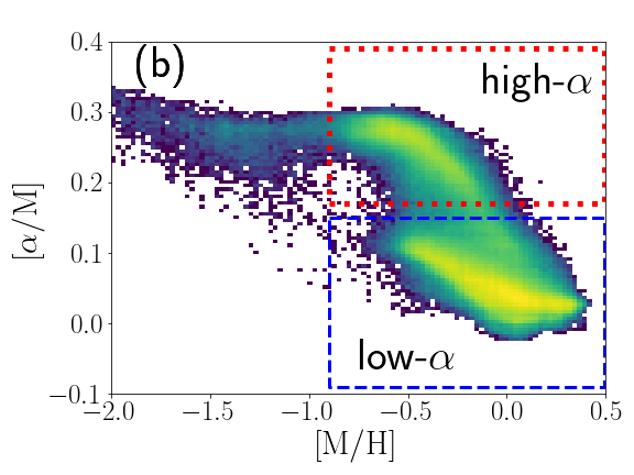
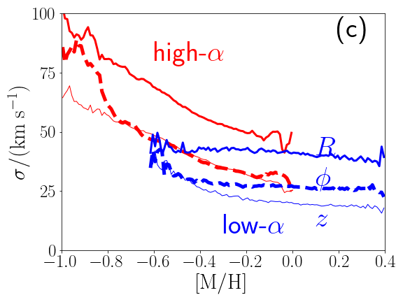
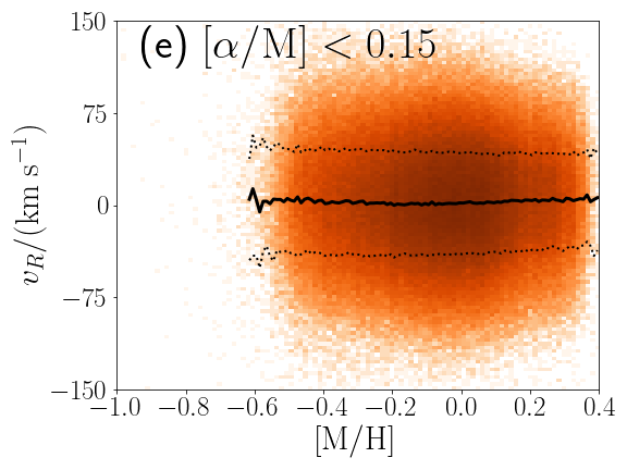
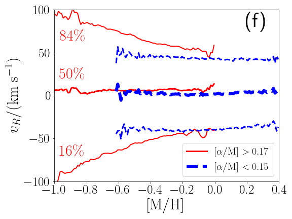
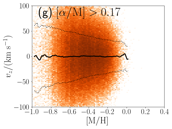
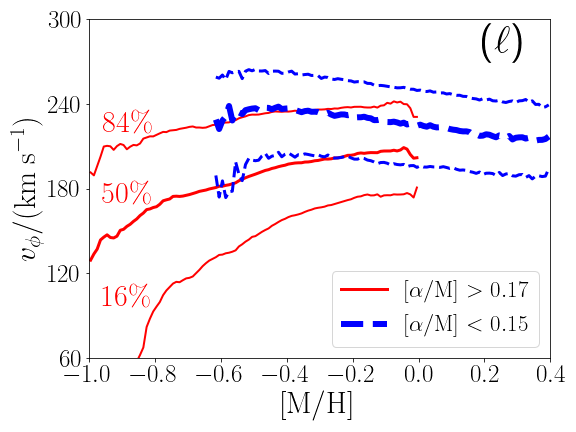
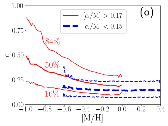
Figure 13: Chemo-dynamics of local giants with high-precision $(\mbox{$\mathrm{[M/H]}$},\mbox{$[\alpha/\mathrm{M}]$})$. (a) CMD selection of giants. (b) Selection box for high-$\alpha$ and low-$\alpha$ stars. (c) Velocity dispersion of high-$\alpha$ and low-$\alpha$ stars as a function of $\mathrm{[M/H]}$ in our catalog. (d)-(f) The distribution of the Galactocentric cylindrical radial velocity $v_{R}$ as a function of $\mathrm{[M/H]}$. (g)-(i) The distribution of the Galactocentric vertical velocity $v_{z}$. (j)-($\ell$) The distribution of the Galactocentric azimuthal velocity $v_{\phi}$. (m)-(o) The distribution of the orbital eccentricity $e$. In panels (d)-(o), the three lines correspond to the 16th, 50th, and 84th percentile values.

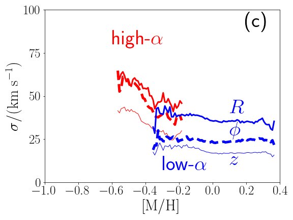
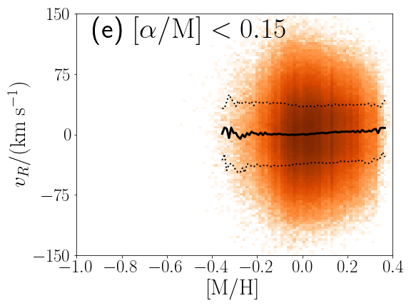
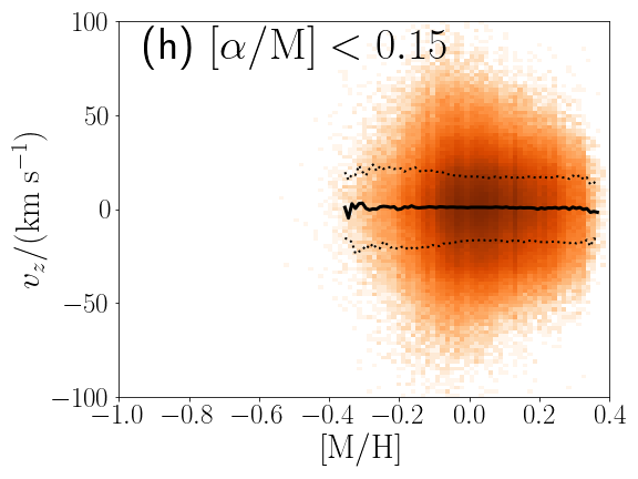
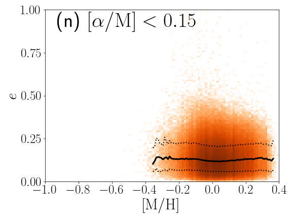
Figure 14: The same as Fig. 13, but for local low-temperature dwarfs in our catalog. We note that the chemo-dynamical correlations for the low-temperature dwarfs (right-most column of this figure) are similar to those for giants (right-most column of Fig. 13). This result is a supporting evidence that, at high-metallicity region (e.g., $\mbox{$\mathrm{[M/H]}$}>-0.6$) our estimates of ($\mathrm{[M/H]}$, $[\alpha/\mathrm{M}]$) for the high-precision subsample of low-temperature dwarfs are reliable.

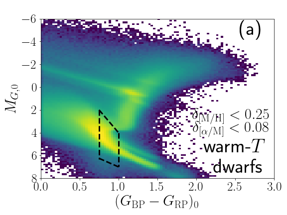
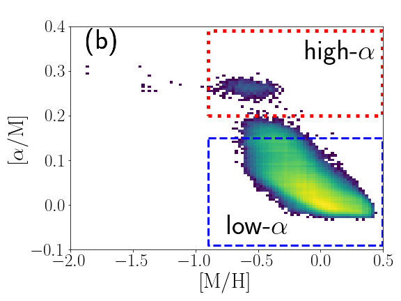
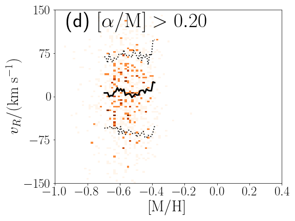
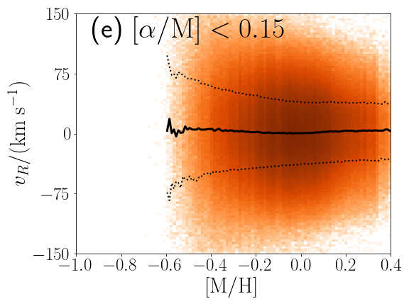
Figure 15: The same as Fig. 13, but for local warm-temperature dwarfs in our catalog. We note that, for the warm-temperature dwarfs, the dynamical properties of high-$\alpha$ stars and low-$\alpha$ stars are similar to each other at their overlapping $\mathrm{[M/H]}$ (i.e., $\mbox{$\mathrm{[M/H]}$}\simeq-0.5$). This result is in contrast to the result for giants and low-temperature dwarfs. This result implies that our estimates of $[\alpha/\mathrm{M}]$ for warm-temperature dwarfs may be less reliable than those for giants and low-temperature dwarfs.

6 Interpretation of the QRF models

To better understand/interpret how our models work, we conduct an additional analysis using the grouped Permutation Feature Importance (gPFI) method. We note that the analysis in this Section is independent from the main analysis in this paper.

6.1 Simple QRF models

In the main analysis of this paper, we construct our models that use the 1310-dimensional data vector $X=(\mbox{\boldmath$C$},\mbox{\boldmath$F$}_{\mathrm{BP}},\mbox{\boldmath$F$}_{\mathrm{RP}})$ as their inputs. In this Section, we construct simpler models in the same manner as in Section 3 except that we use a 1200-dimensional data vector

$$X=(\mbox{\boldmath$F$}_{\mathrm{BP}},\mbox{\boldmath$F$}_{\mathrm{RP}}).$$ (14)

Because the information of the normalized spectral coefficients $C$ and that of the normalized mean BP and RP spectra $(\mbox{\boldmath$F$}_{\mathrm{BP}},\mbox{\boldmath$F$}_{\mathrm{RP}})$ are redundant (see Fig. 1), removing $C$ from $X$ makes the interpretation of the model more transparent. Following Section 3, we separately train a model to estimate $\mathrm{[M/H]}$ (Simple-QRF-MH model) and another model to estimate $[\alpha/\mathrm{M}]$ (Simple-QRF-AM model).

As in Section 4.1, we apply the Simple-QRF-MH model and Simple-QRF-AM model to the test data and evaluate the RMSE values. We find that the RMSE values are $0.119$ dex for $\mathrm{[M/H]}$ and $0.0556$ dex for $[\alpha/\mathrm{M}]$, when we use the entire test data. In the following, we will analyze the Simple-QRF-MH and Simple-QRF-AM models.

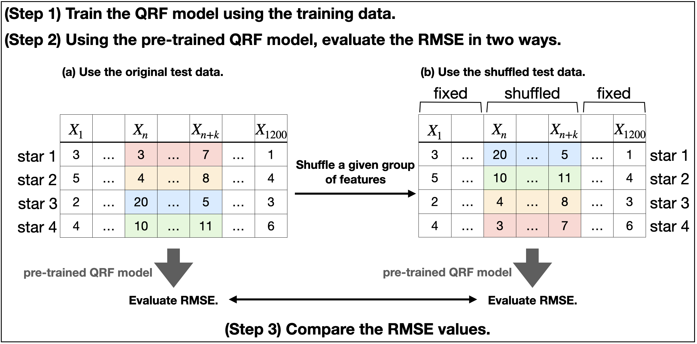
Figure 16: The schematic explanation of gPFI analysis. We make a shuffled test data in which the grouped features $(X_{n},\cdots,X_{n+k})$ are shuffled randomly. (We do not shuffle the labels in the test data.) If the grouped features $(X_{n},\cdots,X_{n+k})$ are important, shuffling them would make the prediction worse. Thus, by investigating the ratio of the RMSE in (b) to the RMSE in (a), we can evaluate the importance of the grouped features.

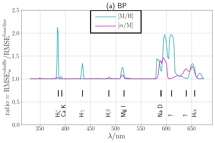
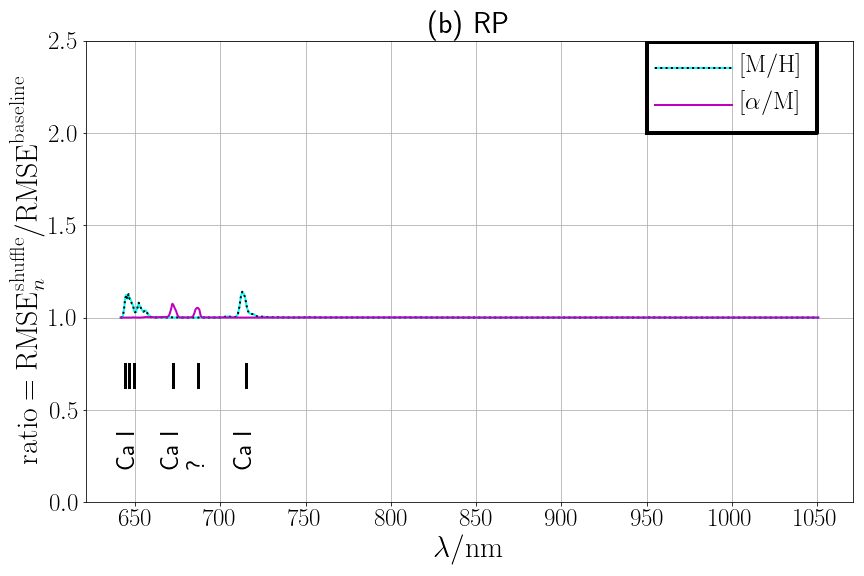
Figure 17: The importance of each wavelength range in the XP spectra in inferring the labels ($\mathrm{[M/H]}$, $[\alpha/\mathrm{M}]$) estimated from the gPFI analysis. The vertical axis ($\mathrm{ratio}=\mathrm{RMSE}^{\mathrm{shuffle}}_{n}/\mathrm{RMSE}^{\mathrm{baseline}}$) indicates how the performance of the ML models deteriorate if the flux data near a given wavelength region are shuffled. In panels (a) The results for BP and RP spectra are shown in panels (a) and (b), respectively. We also plot the locations of some important absorption lines. We note that the BP spectra contain much more information than RP spectra. Intriguingly, our model seem to extract information on $[\alpha/\mathrm{M}]$ from the spectral shape near Na D lines (at 589.0 nm and 589.6 nm).

6.2 gPFI analysis

The procedure of the gPFI analysis is schematically described in Fig. 16. For simplicity, let us focus on the procedure for the Simple-QRF-MH model. As we have mentioned in the previous subsection, this model has a RMSE in $\mathrm{[M/H]}$ of 0.119 dex when applied to the test data set. We use this value as the baseline value, $\mathrm{RMSE}^{\mathrm{baseline}}$. In the gPFI analysis, we apply this pre-trained Simple-QRF-MH model to a ‘shuffled’ test data set. To be specific, among the 1200-dimensional information of $X$, we combine $k$ consecutive features $\{X_{n},\cdots,X_{n+k}\}$ as a group, and shuffle this group of features in the test data to create a shuffled test data set. In the shuffled test data, the stellar labels are not shuffled. We then compute the RMSE value for the shuffled test data (denoted as $\mathrm{RMSE}^{\mathrm{shuffled}}_{n}$) and compare the value with the baseline value $\mathrm{RMSE}^{\mathrm{baseline}}$.

The interpretation of the gPFI method is simple. On the one hand, suppose that the shuffled features do not contain any information on $\mathrm{[M/H]}$. In this case, shuffling them would result in almost identical RMSE value ($\mathrm{RMSE}^{\mathrm{shuffled}}_{n}/\mathrm{RMSE}^{\mathrm{baseline}}\simeq 1$). On the other hand, suppose that the shuffled features contain some useful information on $\mathrm{[M/H]}$. In this case, shuffling them would increase the RMSE value (i.e., deteriorate the prediction of $\mathrm{[M/H]}$), so that the ratio $\mathrm{RMSE}^{\mathrm{shuffled}}_{n}/\mathrm{RMSE}^{\mathrm{baseline}}$ becomes notably larger than 1. The gPFI analysis measures the importance of the grouped features by measuring how the RMSE increases due to the shuffling.

We remind that $X$ is the normalized flux value sampled at 1200 points in the pseudo-wavelength range. Thus, $\{X_{n},\cdots,X_{n+k}\}$ corresponds to the normalized flux at a certain wavelength region within the BP band if $n+k\leq 600$, and within the RP band if $601\leq n$. In our analysis, we choose integer values at $132\leq n\leq 510$ (BP domain; corresponding to $680\geq\lambda/\mathrm{nm}\geq 330$) and $733\leq n\leq 1107$ (RP domain; corresponding to $640\leq\lambda/\mathrm{nm}\leq 1050$). We also set $k=5$, but the choice of $k$ only has a small effect on the result.

6.3 Results of gPFI analysis

We conduct the gPFI analysis for Simple-QRF-MH model and Simple-QRF-AM model, as shown in Fig. 17. In Fig. 17, the horizontal axis is the physical wavelength that is converted from the pseudo wavelength (see Fig. 1). (To be specific, we compute the $n$th and $(n+k)$th wavelengths and use the mean value as the horizontal axis.) The vertical axis is evaluated by

$$\mathrm{(ratio)}=\mathrm{RMSE}^{\mathrm{shuffled}}_{n}/\mathrm{RMSE}^{\mathrm{baseline}}.$$ (15)

This ratio is notably larger than $1$ if the shuffled wavelength range contains some information on the label ($\mathrm{[M/H]}$ or $[\alpha/\mathrm{M}]$). This ratio should be $1$ if the shuffled wavelength range does not contain any information on the label.

From Fig. 17, we see that our models extract information on ($\mathrm{[M/H]}$, $[\alpha/\mathrm{M}]$) from several narrow wavelength regions, mostly in the BP spectra. Importantly, a large portion of the information on $[\alpha/\mathrm{M}]$ seem to arise from the spectral feature near the Na D lines (at 589.0 nm and 589.6 nm). As demonstrated in Appendix C, there is an observational trend such that stars with higher [Na/Fe] tend to have higher [Mg/Fe] for a given metallicity [Fe/H]. Thus, we interpret that our Simple-QRF-AM model probably extracts information on $[\alpha/\mathrm{M}]$ from the Na D lines through this correlation. Fig. 17(a) indicates that the Mg I line at 516 nm is also used to infer $[\alpha/\mathrm{M}]$. Therefore, reassuringly, our Simple-QRF-AM model is not entirely dependent on the data near the Na D lines.

Interestingly, the same Mg I line is also used by our Simple-QRF-MH model to infer $\mathrm{[M/H]}$. This result means that the Simple-QRF-MH model is using the correlation between the Mg abundance and the overall metal abundance. Also, Fig. 17(a) indicates that some H-lines (e.g., H$\zeta$ and H$\gamma$) are also used to extract information on $\mathrm{[M/H]}$.

The gPFI analysis is helpful for humans to understand how the ML models extract information on ($\mathrm{[M/H]}$, $[\alpha/\mathrm{M}]$). However, we have some wavelength regions for which we do not fully understand why the models find useful (or useless). For example, we see a notable features at 610 nm and 639 nm in Fig. 17(a) or at 687 nm in Fig. 17(b), but we do not understand why these wavelength regions are more important than other wavelength regions. As another example, we do not see any features in Fig. 17(b) near the Ca triplet lines (at 849.8 nm, 854.2 nm, and 866.2 nm), although we know that Ca triplet is a strong absorption feature which has long been used to infer ($\mathrm{[M/H]}$, $[\alpha/\mathrm{M}]$) from high-resolution spectroscopy.

We note that the gPFI analysis in this Section is based on Simple-QRF-MH and Simple-QRF-AM models, which are trained on 1200-dimensional data. These models are technically different from QRF-MH and QRF-AM models in the main analysis of this paper, which are trained on 1310-dimensional data (see Fig. 1). However, we believe that the interpretation of the models obtained in this Section is applicable to the QRF-MH and QRF-AM models as well, because the models are quite similar to each other. (For example, we can naturally guess that QRF-AM model also uses the Na D lines to infer $[\alpha/\mathrm{M}]$.) We note that gPFI analysis is just one of many tools to interpret the ML models, and we should try other tools to try to understand the ML models. In the future, we hope that our gPFI analysis may serve as a useful starting point to understand the blurred information encoded in the Gaia XP spectra.

7 Conclusion

In this paper, we use a tree-based ML algorithm to infer ($\mathrm{[M/H]}$, $[\alpha/\mathrm{M}]$) from the low-resolution Gaia XP spectra. The estimation of $\mathrm{[M/H]}$ from XP spectra have been tried by various groups (e.g., Rix et al. 2022; Andrae et al. 2023; Leung & Bovy 2023), but the estimation of $[\alpha/\mathrm{M}]$ from XP spectra has been recognized as a difficult task, based on theoretical arguments (Gavel et al., 2021; Witten et al., 2022). Prior to our work, only one group tackled this task (Li et al. 2023; but see also Guiglion et al. 2024), who used a modern ML architecture. The uniqueness of this paper is that we tackled this problem by using a classical, tree-based ML algorithm, which allows us to interpret our models in a straightforward manner. This paper is summarized as follows.

1. We separately construct a model to infer $\mathrm{[M/H]}$ (QRF-MH model) and a model to infer $[\alpha/\mathrm{M}]$ (QRF-AM model), by using the training data of giants and dwarfs with known chemistry (Abdurro’uf et al., 2022; Li et al., 2022) located in low dust extinction regions with $E(B-V)<0.1$. In the main analysis, we use 1310-dimensional information of the Gaia XP spectra (shown in Fig. 1), consisting of the 110-dimensional coefficient data and the 1200-dimensional flux data. The derived catalog is available at the Zenodo database (https://zenodo.org/records/10902172).

2. We investigate the performance of our models by using the test data. The RMSE values for our models (which indicate the typical accuracy of our models) are 0.0890 dex for $\mathrm{[M/H]}$ and 0.0436 dex for $[\alpha/\mathrm{M}]$. The accuracy in $\mathrm{[M/H]}$ is comparable to the accuracy in previous works (e.g., Rix et al. 2022; Andrae et al. 2023; Leung & Bovy 2023). The accuracy in $[\alpha/\mathrm{M}]$ is also comparable to the accuracy in Li et al. (2022), who used a modern ML architecture. We note that our models are only applicable to stars with low dust extinction, while other previous models (e.g., Rix et al. 2022; Zhang et al. 2023; Li et al. 2023) are applicable to stars with high dust extinction as well. However, we note that these previous studies used not only the Gaia XP spectra and Gaia’s photometric information but also the parallax information or photometric data from external catalogs. In contrast, we only used Gaia XP spectra and $G$-band magnitude, without using other information. Improving the classical models’ performance for stars with high dust extinction by using external data is the scope for future studies.

3. As summarized in Table 1, our models are more reliable for metal-rich stars ($\mbox{$\mathrm{[M/H]}$}>-1$) than for metal-poor stars ($\mbox{$\mathrm{[M/H]}$}<-1$). This is mainly because we have less training stars with low $\mathrm{[M/H]}$. In the future, it would be important to increase the number of low-$\mathrm{[M/H]}$ stars (with known $[\alpha/\mathrm{M}]$) in the training sample.

4. Our estimates of ($\mathrm{[M/H]}$, $[\alpha/\mathrm{M}]$) are most reliable for giants (see Table 1 and the second row in Figs. 6, 7, 25, and 26). This is mainly because our training data are dominated by giants. The ($\mathrm{[M/H]}$, $[\alpha/\mathrm{M}]$)-distribution obtained from our analysis shows a clear bimodal feature of high-$\alpha$ and low-$\alpha$ sequence. The bimodality is more prominent if we select the high-precision subsample with smaller uncertainty in ($\mathrm{[M/H]}$, $[\alpha/\mathrm{M}]$). Intriguingly, as seen in Fig. 13, the low-$[\alpha/\mathrm{M}]$ and high-$[\alpha/\mathrm{M}]$ stars show distinct kinematics, consistent with the results in the literature (e.g., Lee et al. 2011). This chemo-dynamical correlation is a supporting evidence that our estimates of ($\mathrm{[M/H]}$, $[\alpha/\mathrm{M}]$) are reliable (see also Li et al. (2023), who also used this argument to validate their estimates of ($\mathrm{[M/H]}$, $[\alpha/\mathrm{M}]$) from XP spectra).

5. Our estimates of ($\mathrm{[M/H]}$, $[\alpha/\mathrm{M}]$) are less reliable for dwarfs than for giants (see Table 1). However, we see a positive correlation between our prediction of $\mathrm{[M/H]}$ (or $[\alpha/\mathrm{M}]$) and the spectroscopically determined $\mathrm{[M/H]}$ (or $[\alpha/\mathrm{M}]$), as seen in the third and fourth row in Figs. 6 and 7. Because we have small number of dwarfs in the APOGEE DR17 catalog, we used GALAH DR3 data as the ‘external’ test data to evaluate the performance of dwarfs. As seen in the third and fourth row in Figs. 25 and 26, our models predict reasonable ($\mathrm{[M/H]}$, $[\alpha/\mathrm{M}]$) for dwarfs as well. In the future, it would be interesting to include the GALAH data in the training sample so that the model performance can be improved for dwarfs.

6. The chemo-dynamical correlation seen for giants are also confirmed for low-temperature dwarfs (see Fig. 14). This chemo-dynamical correlation serves as a supporting evidence that our estimates of ($\mathrm{[M/H]}$, $[\alpha/\mathrm{M}]$) are informative for low-temperature dwarfs. In contrast, the chemo-dynamical correlation is not seen for warm-temperature dwarfs (see Fig. 15). This result is at odds with the apparently good performance of our models on warm dwarfs that we see in Figs. 6, 7, 25 and 26. Given the theoretical arguments on the difficulty of inferring $[\alpha/\mathrm{M}]$ for warm-temperature dwarfs (Witten et al., 2022), we need to be careful in using ($\mathrm{[M/H]}$, $[\alpha/\mathrm{M}]$) for warm dwarfs estimated from the XP spectra.

7. To understand how our models infer ($\mathrm{[M/H]}$, $[\alpha/\mathrm{M}]$), we quantify which part of the input XP spectra are important by using a so-called gPFI method (Section 6). In this analysis, we separately construct a model to infer $\mathrm{[M/H]}$ (Simple-QRF-MH model) and a model to infer $[\alpha/\mathrm{M}]$ (Simple-QRF-AM model), by using the 1200-dimensional flux information of the Gaia XP spectra (shown in Fig. 1). We find that the information on ($\mathrm{[M/H]}$, $[\alpha/\mathrm{M}]$) is contained in several narrow wavelength regions, many of which are located within the blue part of the XP spectra. Importantly, $[\alpha/\mathrm{M}]$ seems to be inferred from the Na D lines (589 nm) and the Mg I line (516 nm). This finding is intriguing because the correlation between Na and Mg abundances is known from literature (see Fig. 27) and Mg is a typical $\alpha$ element. Identifying the wavelength ranges that are useful to infer chemistry may be useful in the future to derive chemical abundances from the narrow-band photometric data from large surveys, such as Pristine survey (Martin et al., 2023) or J-PLUS/S-PLUS survey (Yang et al., 2022).

8. Various medium/high-resolution spectroscopic surveys are ongoing or forthcoming, including, but not limited to WEAVE (Jin et al., 2023), 4MOST (de Jong et al., 2019), and PFS (Takada et al., 2014). These massive datasets would provide useful training data to further refine our ML models, which would be beneficial in understanding the chemical distribution within the Milky Way.

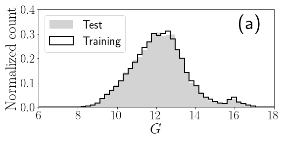
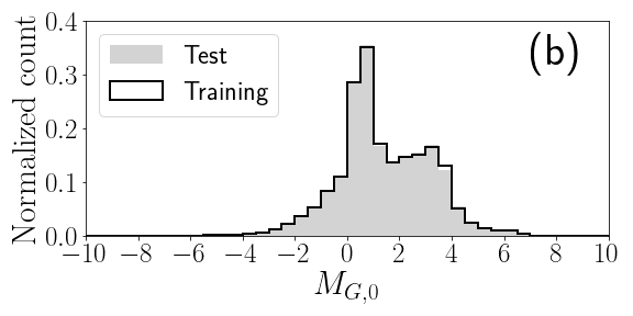
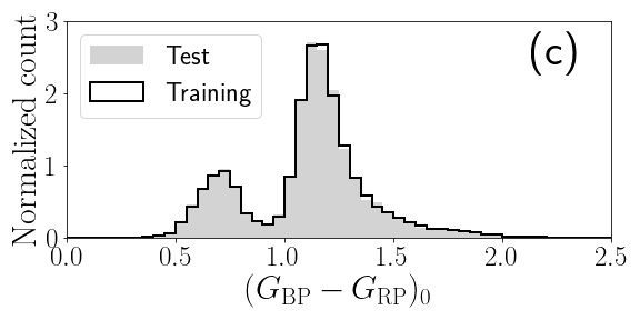
Figure 18: The distribution of stars in our training and test data in the photometric space.

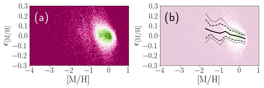
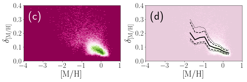
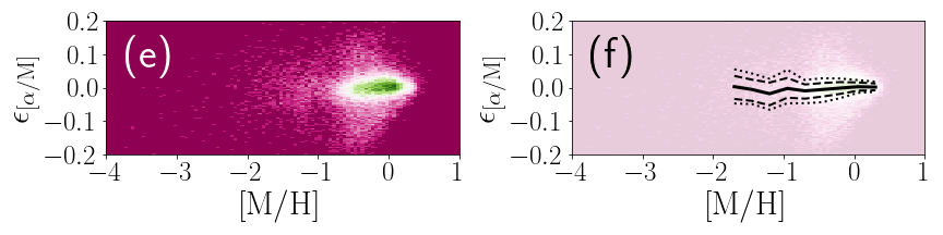
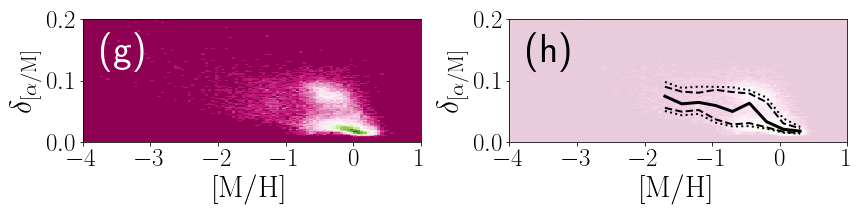
Figure 19: The performance of our QRF models for $\mathrm{[M/H]}$ (panels (a)-(d)) and for $[\alpha/\mathrm{M}]$ (panels (e)-(h)) as a function of metallicity $\mathrm{[M/H]}$, estimated by using the test data. The accuracy of our models (as a function of $\mathrm{[M/H]}$) can be inferred from the median value of $\epsilon_{\mathrm{[M/H]}}$ or $\epsilon_{[\alpha/\mathrm{M}]}$. The precision of our models (as a function of $\mathrm{[M/H]}$) can be inferred from the width of the distribution of $\epsilon_{\mathrm{[M/H]}}$ or $\epsilon_{[\alpha/\mathrm{M}]}$. The precision of $\mathrm{[M/H]}$ or $[\alpha/\mathrm{M}]$ of a star can be inferred from the value of $\delta_{\mathrm{[M/H]}}$ or $\delta_{[\alpha/\mathrm{M}]}$ of each star. (a) The distribution of $\epsilon_{\mathrm{[M/H]}}$, color-coded by the density in the $(\mbox{$\mathrm{[M/H]}$},\mbox{$\epsilon_{\mathrm{[M/H]}}$})$-space. (b) The 16, 25, 50, 75, and 84th percentile values of $\epsilon_{\mathrm{[M/H]}}$ as a function of $\mathrm{[M/H]}$ are shown on top of the density plot. (c) The distribution of $\delta_{\mathrm{[M/H]}}$, color-coded by the density in the $(\mbox{$\mathrm{[M/H]}$},\mbox{$\epsilon_{\mathrm{[M/H]}}$})$-space. (d) The 16, 25, 50, 75, and 84th percentile values of $\delta_{\mathrm{[M/H]}}$ as a function of $\mathrm{[M/H]}$ are shown on top of the density plot. (e) The same as panel (a), but for $\epsilon_{[\alpha/\mathrm{M}]}$. (f) The same as panel (b), but for $\epsilon_{[\alpha/\mathrm{M}]}$. (g) The same as panel (c), but for $\delta_{[\alpha/\mathrm{M}]}$. (h) The same as panel (d), but for $\delta_{[\alpha/\mathrm{M}]}$.

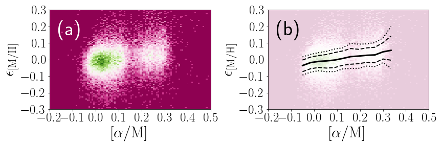
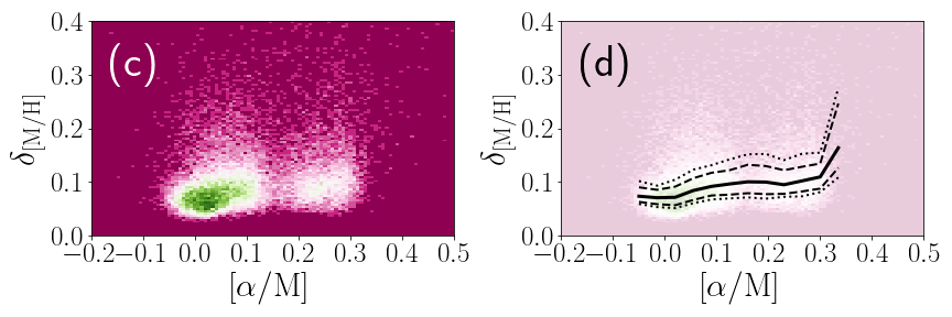
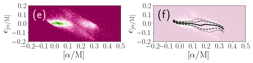
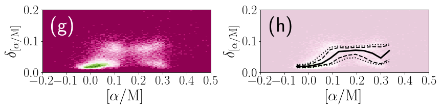
Figure 20: The same as Fig. 19, but as a function of the metallicity $[\alpha/\mathrm{M}]$.

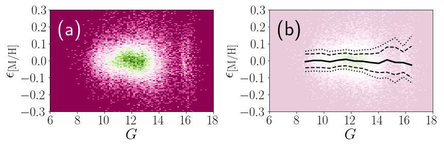
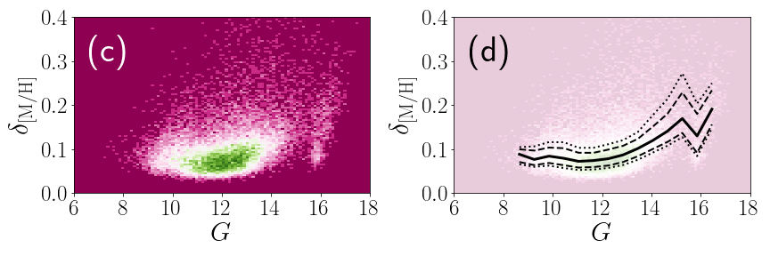
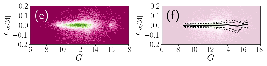
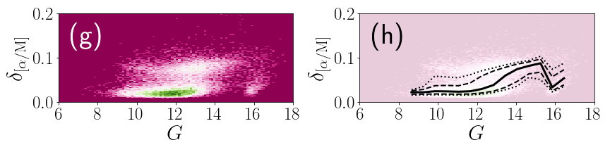
Figure 21: The same as Fig. 19, but as a function of the apparent magnitude $G$.

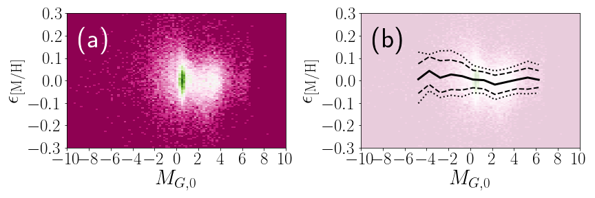
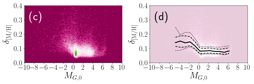
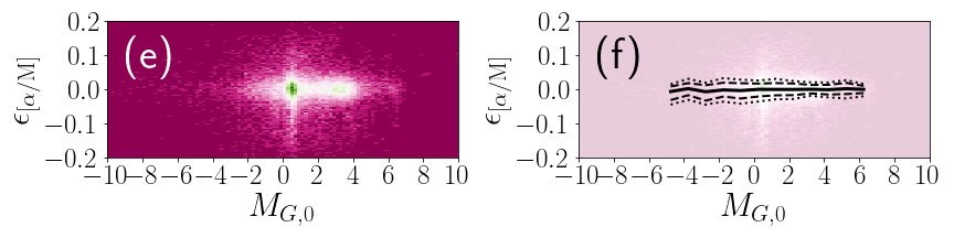
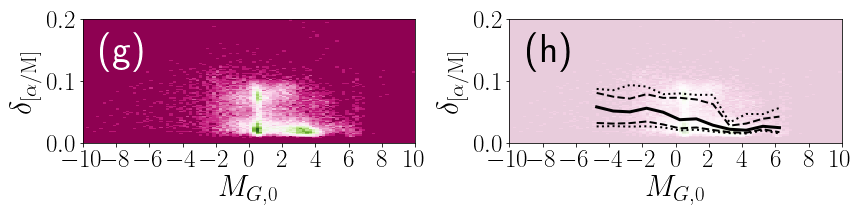
Figure 22: The same as Fig. 19, but as a function of the absolute magnitude $M_{G,0}$.

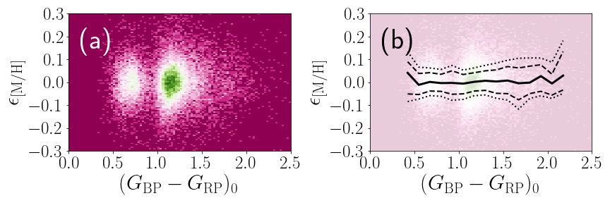
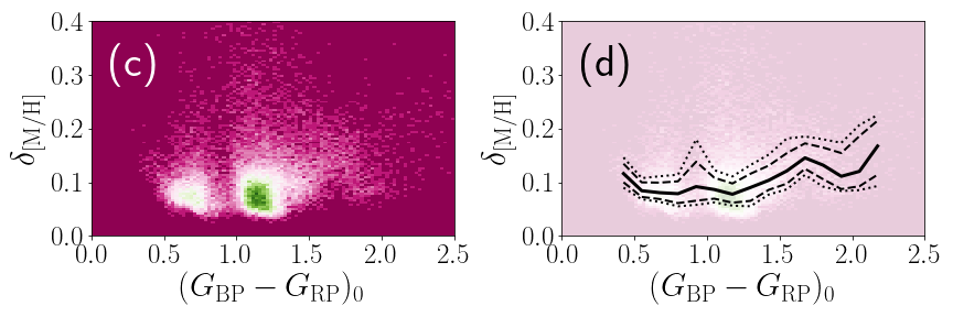
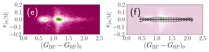
Figure 23: The same as Fig. 19, but as a function of the color $(G_{\mathrm{BP}}-G_{\mathrm{RP}})_{0}$

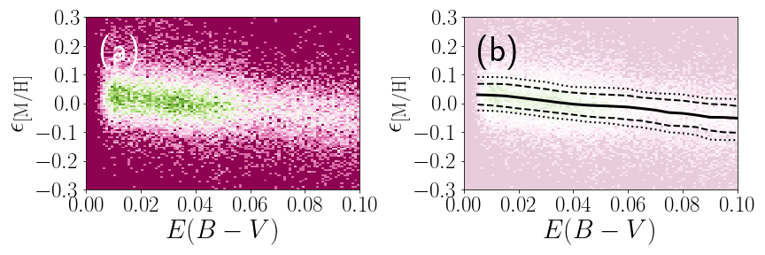
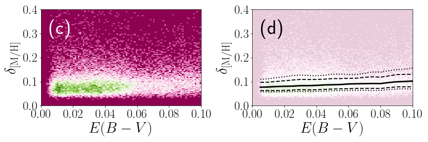
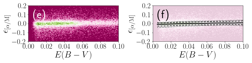
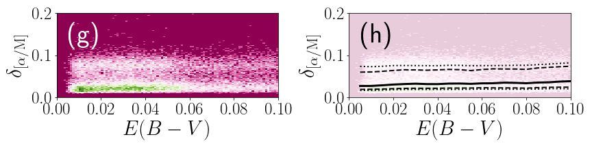
Figure 24: The same as Fig. 19, but as a function of the color excess $E(B-V)$.

Appendix A How the performance of our models depends on the stellar properties

A.1 Dependence on $\mathrm{[M/H]}$

Fig. 19 shows the performance of our models as a function of the metallicity $\mathrm{[M/H]}$. In Fig. 19(b), we show the 16, 25, 50, 75, and 84th percentile values of $\epsilon_{\mathrm{[M/H]}}$ as a function of $\mathrm{[M/H]}$. We see that the median value of $\epsilon_{\mathrm{[M/H]}}$ (solid line) increases as $\mathrm{[M/H]}$ decreases, from $\mbox{$\epsilon_{\mathrm{[M/H]}}$}\simeq-0.02$ at $\mbox{$\mathrm{[M/H]}$}\simeq 0$ to $\mbox{$\epsilon_{\mathrm{[M/H]}}$}\simeq 0.1$ at $\mbox{$\mathrm{[M/H]}$}\simeq-2$. At $-0.8\lesssim\mbox{$\mathrm{[M/H]}$}\lesssim+0.3$, where we have large number of training data, the median value of $\epsilon_{\mathrm{[M/H]}}$ stays near zero, suggesting that there is no strong systematic error in $\mathrm{[M/H]}$ in this region. In contrast, at the low metallicity region ($-2\lesssim\mbox{$\mathrm{[M/H]}$}\lesssim-1$), where we have a smaller number of training data, our model systematically overestimates $\mathrm{[M/H]}$ by up to $\sim 0.1$ dex. At the very-low-metallicity region ($\mbox{$\mathrm{[M/H]}$}\lesssim-2$), where we have few training data or test data, we do not have a reliable way to evaluate the accuracy of our model. However, by extrapolating the trend at $-2\lesssim\mbox{$\mathrm{[M/H]}$}\lesssim-1$, we believe that the accuracy of $\mathrm{[M/H]}$ should be worse.

In Fig. 19(b), the half-width between the 16th and 84th percentiles (half-width between the two dotted lines) roughly corresponds to the typical precision of $\mathrm{[M/H]}$ as a function of $\mathrm{[M/H]}$. We see that the precision of $\mathrm{[M/H]}$ becomes worse as $\mathrm{[M/H]}$ decreases, especially at $\mbox{$\mathrm{[M/H]}$}<-1$. In contrast, at $-0.8\lesssim\mbox{$\mathrm{[M/H]}$}\lesssim+0.3$, the precision of $\mathrm{[M/H]}$ of our model is as good as $\sim 0.05$ dex.

The precision of $\mathrm{[M/H]}$ can be also evaluated by using $\delta_{\mathrm{[M/H]}}$. Fig. 19(d) shows the 16, 25, 50, 75, and 84th percentile values of $\delta_{\mathrm{[M/H]}}$ as a function of $\mathrm{[M/H]}$. We see that the precision becomes worse at $\mbox{$\mathrm{[M/H]}$}<-1$, and it becomes better as $\mathrm{[M/H]}$ increases from $\mbox{$\mathrm{[M/H]}$}\simeq-1$ to $\mbox{$\mathrm{[M/H]}$}\simeq+0.3$.

In Fig. 19(f), we show the 16, 25, 50, 75, and 84th percentile values of $\epsilon_{[\alpha/\mathrm{M}]}$ as a function of $\mathrm{[M/H]}$. The median value of $\epsilon_{[\alpha/\mathrm{M}]}$ stays almost zero at $-2\lesssim\mbox{$\mathrm{[M/H]}$}\lesssim+0.3$, which indicates that there is no strong systematic error on $[\alpha/\mathrm{M}]$ as a function of $\mathrm{[M/H]}$. (This result is in contrast to the behavior of $\epsilon_{\mathrm{[M/H]}}$ mentioned above.) The precision of $[\alpha/\mathrm{M}]$, as measured by the gap between the 16th and 84th percentile values of $[\alpha/\mathrm{M}]$, becomes worse as $\mathrm{[M/H]}$ decreases, which is probably because of the lack of training data at the low metallicity region.

In Fig. 19(g), we see a bimodal distribution of stars in the $(\mbox{$\mathrm{[M/H]}$},\mbox{$\delta_{[\alpha/\mathrm{M}]}$})$-space, which is reminiscent of the two-peak histogram of $\delta_{[\alpha/\mathrm{M}]}$ in Fig. 5 or the off-diagonal distribution of stars in Fig. 7(a)(e). We think that these structures arise because our models sometimes identify low-$\alpha$ stars as high-$\alpha$ stars and vice versa (as discussed in Section 4.2.3).

A.2 Dependence on $[\alpha/\mathrm{M}]$

Fig. 20 shows the performance of our models as a function of the metallicity $[\alpha/\mathrm{M}]$. Fig. 20 is identical to Fig. 19 except that the horizontal axis is $[\alpha/\mathrm{M}]$ in all panels. Fig. 20(b) suggests that $\epsilon_{\mathrm{[M/H]}}$ mildly increases as $[\alpha/\mathrm{M}]$ increases, while $\mbox{$\epsilon_{\mathrm{[M/H]}}$}\simeq 0$ at $\mbox{$[\alpha/\mathrm{M}]$}\simeq 0.1$. This result means that our estimates of $\mathrm{[M/H]}$ for low-$\alpha$ stars are slightly more metal-poor than they should be, and our estimates of $[\alpha/\mathrm{M}]$ for high-$\alpha$ stars are slightly more metal-rich than they should be. In any case, the mild trend and the near-zero value of $\epsilon_{\mathrm{[M/H]}}$ indicate that the systematic error in $\mathrm{[M/H]}$ associated with our model prediction only weakly depends on $[\alpha/\mathrm{M}]$.

Fig. 20(d) suggests that $\delta_{\mathrm{[M/H]}}$ mildly increases as $[\alpha/\mathrm{M}]$ increases. This result means that the precision in $\mathrm{[M/H]}$ of our model prediction smaller for low-$\alpha$ stars than high-$\alpha$ stars.

Fig. 20(f) suggests that $\epsilon_{[\alpha/\mathrm{M}]}$ very mildly decreases as $[\alpha/\mathrm{M}]$ increases. However, the median value of $\epsilon_{[\alpha/\mathrm{M}]}$ is generally very close to zero, and the half-width between the 16 and 84th percentiles of the distribution of $\epsilon_{[\alpha/\mathrm{M}]}$ is as small as $\simeq 0.03$ dex. Therefore our model can separate high-$\alpha$ and low-$\alpha$ stars in our test data.

In Fig. 20(g), we see a quadruple distribution of stars, which is reminiscent of the off-diagonal distribution of stars in Fig. 7(a)(e) (see discussion in Section 4.2.3).

A.3 Dependence on the apparent magnitude $G$

Fig. 21 shows the performance of our models as a function of the apparent magnitude $G$. In Fig. 21(b), the median value of $\epsilon_{\mathrm{[M/H]}}$ is near zero at $G<13$, suggesting little systematic error in $\mathrm{[M/H]}$ as a function of $G$ at $G<13$. Also, the other percentile values as a function of $G$ are almost unchanged at $G<13$, suggesting that the precision of $\mathrm{[M/H]}$ estimated from our model is almost constant ($\simeq 0.04$ dex) at $G<13$. The precision of $\mathrm{[M/H]}$ becomes worse at fainter magnitudes (except near $G\simeq 16$), consistent with theoretical study by Witten et al. (2022). Interestingly, the precision of $\mathrm{[M/H]}$ is good near $G\simeq 16$. Although $G\simeq 16$ corresponds to a magnitude range where we have a relatively large number of training data (see a bump at $G\simeq 16$ in Fig. 18(a)), we do not have an intuitive understanding on why our models perform better at $G\simeq 16$, because we normalize the flux when we analyze the data.

A similar trend is also seen in Fig. 21(d). Here, the percentile values of $\delta_{\mathrm{[M/H]}}$ are almost constant, but mildly increasing as a function of $G$ at $G<13$. The precision of $\mathrm{[M/H]}$ becomes worse at fainter magnitudes.

In Fig. 21(f), the median value of $\epsilon_{[\alpha/\mathrm{M}]}$ is nearly zero at $9<G<17$, suggesting little systematic error in $[\alpha/\mathrm{M}]$. The precision of $[\alpha/\mathrm{M}]$ inferred from the half-width of the distribution of $\epsilon_{[\alpha/\mathrm{M}]}$ is almost constant ($\simeq 0.02$ dex) as a function of $G$ at $G<13$. The precision of $[\alpha/\mathrm{M}]$ becomes worse at fainter magnitudes (except near $G\simeq 16$).

In Fig. 21(g), we see a bimodal distribution of stars in the $(G,\mbox{$\delta_{[\alpha/\mathrm{M}]}$})$-space at $10<G<15$, which is reminiscent of the bimodal histogram in Fig. 5.

A.4 Dependence on the evolutionary stage $(M_{G,0})$

Our training data include both giants and dwarfs. As shown in Fig. 3, these different evolutionary stages have different absolute magnitude $M_{G,0}$. For example, giants brighter than the red clump stars have $M_{G,0}<0$, red clump stars have $M_{G,0}\simeq 1$, and most dwarfs have $M_{G,0}>3$. Thus, we can evaluate how the the performance of our models depends on the stellar evolutionary stage by dissecting the stars by $M_{G,0}$.

Fig. 22 shows the performance of our models as a function of $M_{G,0}$. As seen from the solid lines in Figs. 22(b) and 22(f), we do not see a systematic error on $\mathrm{[M/H]}$ or $[\alpha/\mathrm{M}]$ for both giants and main-sequence stars, as indicated by the near-zero median value of $\epsilon_{\mathrm{[M/H]}}$ or $\epsilon_{[\alpha/\mathrm{M}]}$.

From Figs. 22(d) and 22(h), there seems to be a tendency that the precision in $\mathrm{[M/H]}$ and $[\alpha/\mathrm{M}]$ are worse for giants than main-sequence stars. However, we need to be cautious in interpreting this result, as this result might be related to the spatial distribution of our training/test data. Dwarfs (or intrinsically faint stars) in the training data are typically located closer to the Sun than giants (or intrinsically bright stars) in the training data. Because nearby stars are dominated by metal-rich, low-$\alpha$ stars (or thin disk stars), there is a possibility that our model might have learned this correlation. As demonstrated by other authors (e.g., Rix et al. 2022; Andrae et al. 2023), the Gaia XP spectra have some information on the stellar surface gravity $\log g$. Thus, we can imagine a situation in which a machine-learning model that returns a high-$\mathrm{[M/H]}$ and low-$[\alpha/\mathrm{M}]$ values for any stars with high-$\log g$ value may look successful in estimating $(\mbox{$\mathrm{[M/H]}$},\mbox{$[\alpha/\mathrm{M}]$})$. In this paper, we do not further investigate this possibility.

A.5 Dependence on the color $(G_{\mathrm{BP}}-G_{\mathrm{RP}})_{0}$

Previous works by Gavel et al. (2021) and Witten et al. (2022) suggested that inferring $[\alpha/\mathrm{M}]$ from the Gaia XP spectra is challenging, except for stars with $\mbox{$T_{\rm eff}$}<5000\;\mathrm{K}$ (which is equivalent to $1.1\gtrsim(G_{\mathrm{BP}}-G_{\mathrm{RP}})_{0}$, based on the mean color-$T_{\rm eff}$ relationship of dwarfs compiled by Eric Mamajek).

Fig. 23 shows the performance of our models as a function of the dereddened color $(G_{\mathrm{BP}}-G_{\mathrm{RP}})_{0}$. As shown in Fig. 18(c), our training data do not have enough stars at $0.8<(G_{\mathrm{BP}}-G_{\mathrm{RP}})_{0}<1.0$. Thus, near this region, the precision of $\mathrm{[M/H]}$ and $[\alpha/\mathrm{M}]$ becomes worse (see Figs. 23(b), 23(d), 23(f), and 23(h)). However, as seen in Fig. 23(f), the precision of $[\alpha/\mathrm{M}]$ look reasonably good at $0.5<(G_{\mathrm{BP}}-G_{\mathrm{RP}})_{0}<0.8$ ($5800\;\mathrm{K}<\mbox{$T_{\rm eff}$}<6800\;\mathrm{K}$).

A.6 Dependence on the color excess $E(B-V)$

As pointed out by Bailer-Jones (2010), the observed shape of the Gaia XP spectra are affected by the dust extinction. Therefore, estimating $(\mbox{$\mathrm{[M/H]}$},\mbox{$[\alpha/\mathrm{M}]$})$ from the XP spectra for stars with high dust extinction is harder than for stars with low dust extinction. This is why we restrict ourselves to stars with low dust extinction: $E(B-V)<0.1$.

Fig. 24 shows the performance of our models as a function of the color excess $E(B-V)$. Fig. 24(b) shows that the median of $\epsilon_{\mathrm{[M/H]}}$ mildly decreases as $E(B-V)$ increases, from $\mbox{$\epsilon_{\mathrm{[M/H]}}$}=+0.03$ at $E(B-V)=0$, through $\mbox{$\epsilon_{\mathrm{[M/H]}}$}=0$ at $E(B-V)=0.04$, to $\mbox{$\epsilon_{\mathrm{[M/H]}}$}=-0.06$ at $E(B-V)=0.10$. We do not have a clear understanding of this trend. Since a star with a larger $E(B-V)$ becomes redder, we naively expect such a star may look more metal-rich (larger $\epsilon_{\mathrm{[M/H]}}$ for larger $E(B-V)$), which is contrary to what we see in Fig. 24(b).

Except for the above-mentioned systematic trend of $\mathrm{[M/H]}$, we see that the performance of our models are not sensitive to $E(B-V)$, as seen from Figs. 24(d), 24(f), and 24(h).

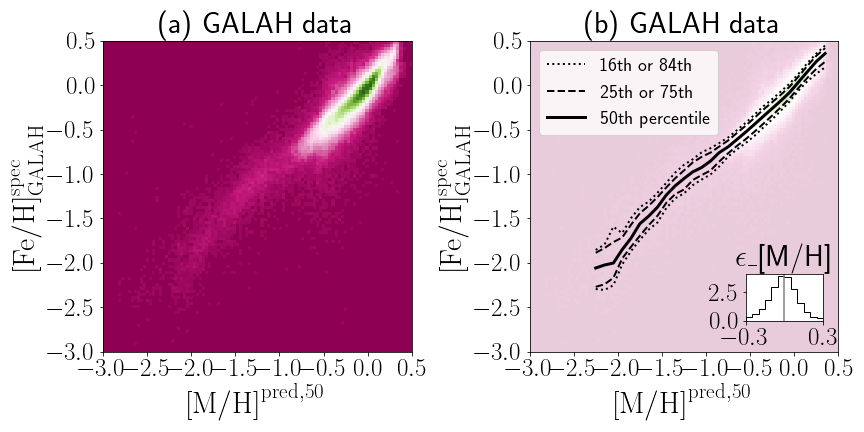
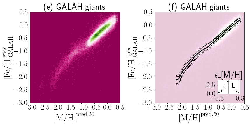
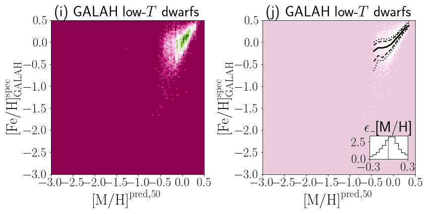
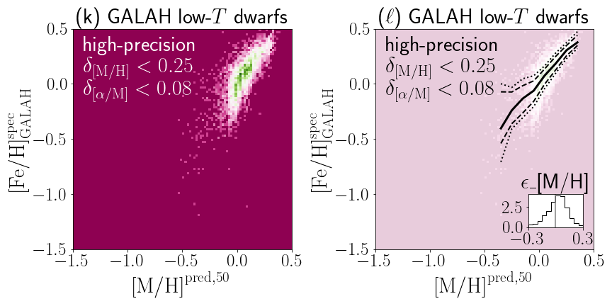
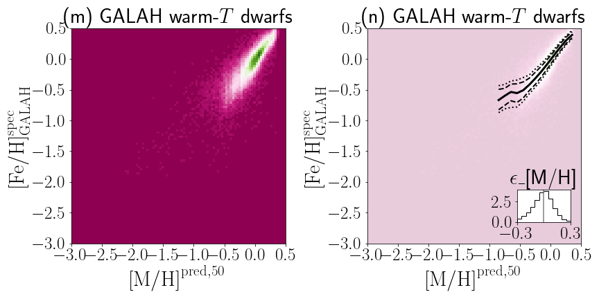
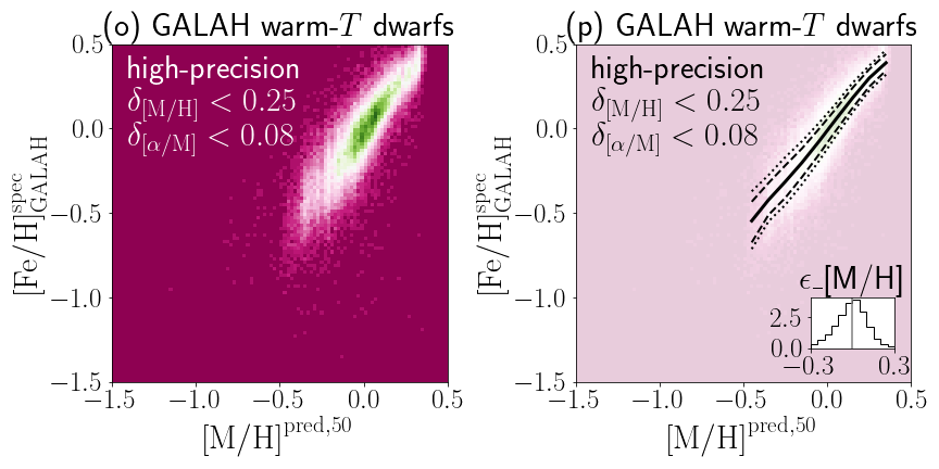
Figure 25: The same as Fig. 6, but showing the detailed performance of the QRF-MH model (our model for estimating $\mathrm{[M/H]}$) applied to the GALAH data.

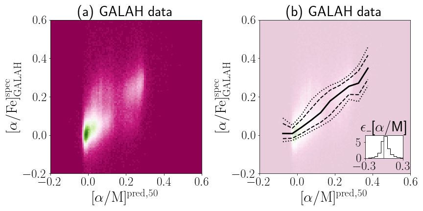
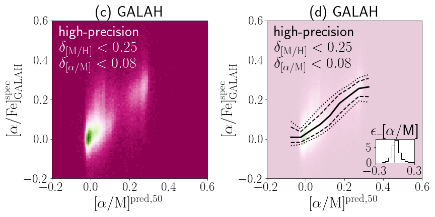
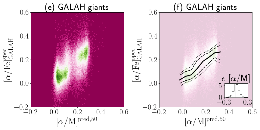
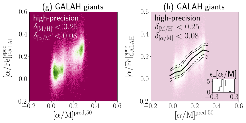
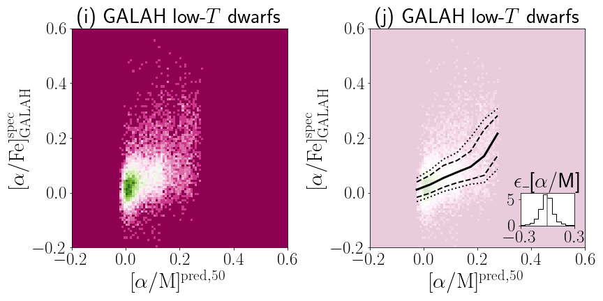
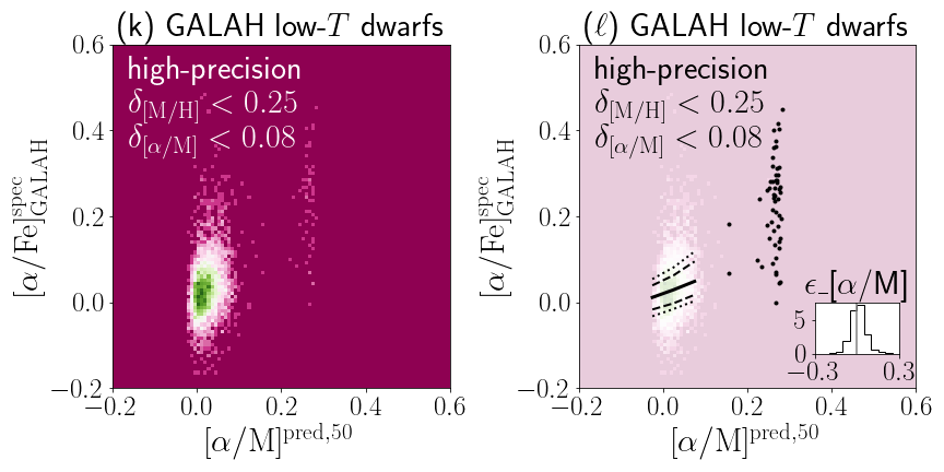
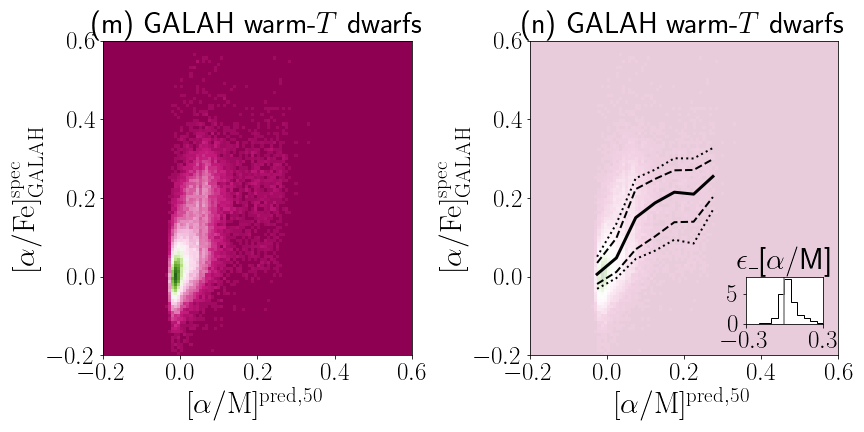
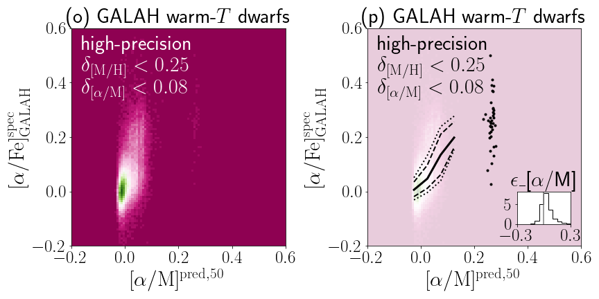
Figure 26: The same as Fig. 6, but showing the detailed performance of the QRF-AM model (our model for estimating $[\alpha/\mathrm{M}]$) applied to the GALAH data. In panels ($\ell$) and (p), we plot the stars with $\mbox{$[\alpha/\mathrm{M}]$}^{\mathrm{pred,50}}>0.15$ with black dots to highlight that the majority of them are genuine high-$\alpha$ stars ($\mbox{$[\alpha/\mathrm{M}]$}^{\mathrm{spec}}_{\mathrm{GALAH}}>0.15$).

Appendix B Validation of our model using the external test data from GALAH DR3

Here we conduct an additional test of our QRF-MH and QRF-AM models with the external test data taken from the GALAH DR3 described in Section 2.3. The analyses are the same as those in Sections 4.2.2 and 4.2.3, but using the GALAH data set. The results are shown in Figs.  25 and 26. We note that we treat [Fe/H] and $[\alpha/\mathrm{Fe}]$ in GALAH DR3 as the proxies for $\mathrm{[M/H]}$ and $[\alpha/\mathrm{M}]$, respectively.

Appendix C Correlation between Na and Mg

Here we briefly describe the observed correlation between Na and Mg abundances. Fig. 27 shows the distribution of ([Fe/H], [Mg/Fe]) and ([Fe/H], [Na/Fe]) of nearby stars taken from the non-local thermodynamic equilibrium analysis by Gehren et al. (2006). To guide the eyes, we divide the sample stars into two groups, by using a simple boundary shown in Fig. 27(a). By definition, for a given [Fe/H], the relatively $\alpha$-rich group is always have higher [Mg/Fe] than the relatively $\alpha$-rich group. With this definition, we see from Fig. 27(b) that the relatively $\alpha$-rich group tend to have higher [Na/Fe] than the relatively $\alpha$-rich group at any given [Fe/H].

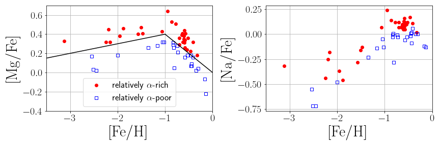
Figure 27: The observed chemical distribution of nearby metal-poor stars taken from (Gehren et al., 2006). We see a correlation between Na and Mg, such that [Na/Fe]-enhanced stars are likely [Mg/Fe]-enhanced for a fixed value of [Fe/H].

Appendix D Coordinate system

We adopt a right-handed Galactocentric Cartesian coordinate system $(x,y,z)$, in which the $(x,y)$-plane is the Galactic disk plane. The position of the Sun is assumed to be $\mbox{\boldmath$x$}_{\odot}=(x_{\odot},y_{\odot},z_{\odot})=(-R_{\odot},0,z_{\odot})$, with $R_{\odot}=8.277\,\mathrm{kpc}$ (GRAVITY Collaboration et al., 2022) and $z_{\odot}=0.0208\,\mathrm{kpc}$ (Bennett & Bovy, 2019). The velocity of the Sun with respect to the Galactic rest frame is assumed to be $\mbox{\boldmath$v$}_{\odot}=(v_{x,\odot},v_{y,\odot},v_{z,\odot})=(9.3,251.5,8.59)\,\mathrm{km\ s}^{-1}$. When we evaluate the orbital eccentricity of stars, we assume the Galactic potential model in McMillan (2017).

References

- Abdurro’uf et al. (2022) Abdurro’uf, Accetta, K., Aerts, C., et al. 2022, ApJS, 259, 35, doi: 10.3847/1538-4365/ac4414
- Andrae et al. (2023) Andrae, R., Rix, H.-W., & Chandra, V. 2023, ApJS, 267, 8, doi: 10.3847/1538-4365/acd53e
- Aoki et al. (2022) Aoki, W., Li, H., Matsuno, T., et al. 2022, ApJ, 931, 146, doi: 10.3847/1538-4357/ac6515
- Bailer-Jones (2010) Bailer-Jones, C. A. L. 2010, MNRAS, 403, 96, doi: 10.1111/j.1365-2966.2009.16125.x
- Bellazzini et al. (2023) Bellazzini, M., Massari, D., De Angeli, F., et al. 2023, A&A, 674, A194, doi: 10.1051/0004-6361/202345921
- Belokurov et al. (2023) Belokurov, V., Vasiliev, E., Deason, A. J., et al. 2023, MNRAS, 518, 6200, doi: 10.1093/mnras/stac3436
- Bennett & Bovy (2019) Bennett, M., & Bovy, J. 2019, MNRAS, 482, 1417, doi: 10.1093/mnras/sty2813
- Buder et al. (2021) Buder, S., Sharma, S., Kos, J., et al. 2021, MNRAS, 506, 150, doi: 10.1093/mnras/stab1242
- Chandra et al. (2023) Chandra, V., Naidu, R. P., Conroy, C., et al. 2023, ApJ, 951, 26, doi: 10.3847/1538-4357/accf13
- Cutri et al. (2021) Cutri, R. M., Wright, E. L., Conrow, T., et al. 2021, VizieR Online Data Catalog, II/328
- De Angeli et al. (2022) De Angeli, F., Weiler, M., Montegriffo, P., et al. 2022, arXiv e-prints, arXiv:2206.06143, doi: 10.48550/arXiv.2206.06143
- de Jong et al. (2019) de Jong, R. S., Agertz, O., Berbel, A. A., et al. 2019, The Messenger, 175, 3, doi: 10.18727/0722-6691/5117
- De Silva et al. (2015) De Silva, G. M., Freeman, K. C., Bland-Hawthorn, J., et al. 2015, MNRAS, 449, 2604, doi: 10.1093/mnras/stv327
- Gaia Collaboration et al. (2022) Gaia Collaboration, Vallenari, A., Brown, A. G. A., et al. 2022, arXiv e-prints, arXiv:2208.00211, doi: 10.48550/arXiv.2208.00211
- Gavel et al. (2021) Gavel, A., Andrae, R., Fouesneau, M., Korn, A. J., & Sordo, R. 2021, A&A, 656, A93, doi: 10.1051/0004-6361/202141589
- Gehren et al. (2006) Gehren, T., Shi, J. R., Zhang, H. W., Zhao, G., & Korn, A. J. 2006, A&A, 451, 1065, doi: 10.1051/0004-6361:20054434
- Gilmore et al. (2012) Gilmore, G., Randich, S., Asplund, M., et al. 2012, The Messenger, 147, 25
- GRAVITY Collaboration et al. (2022) GRAVITY Collaboration, Abuter, R., Aimar, N., et al. 2022, A&A, 657, L12, doi: 10.1051/0004-6361/202142465
- Green (2018) Green, G. 2018, The Journal of Open Source Software, 3, 695, doi: 10.21105/joss.00695
- Green et al. (2018) Green, G. M., Schlafly, E. F., Finkbeiner, D., et al. 2018, MNRAS, 478, 651, doi: 10.1093/mnras/sty1008
- Guiglion et al. (2024) Guiglion, G., Nepal, S., Chiappini, C., et al. 2024, A&A, 682, A9, doi: 10.1051/0004-6361/202347122
- Hastie et al. (2001) Hastie, T., Tibshirani, R., & Friedman, J. 2001, The Elements of Statistical Learning, Springer Series in Statistics (New York, NY, USA: Springer New York Inc.)
- Hunter (2007) Hunter, J. D. 2007, Computing in Science and Engineering, 9, 90, doi: 10.1109/MCSE.2007.55
- Jin et al. (2023) Jin, S., Trager, S. C., Dalton, G. B., et al. 2023, MNRAS, doi: 10.1093/mnras/stad557
- Jones et al. (2001) Jones, E., Oliphant, T., & Peterson, P., e. a. 2001, SciPy: Open source scientific tools for Python. http://www.scipy.org/
- Laroche & Speagle (2023) Laroche, A., & Speagle, J. S. 2023, arXiv e-prints, arXiv:2307.06378, doi: 10.48550/arXiv.2307.06378
- Lee et al. (2011) Lee, Y. S., Beers, T. C., An, D., et al. 2011, ApJ, 738, 187, doi: 10.1088/0004-637X/738/2/187
- Leung & Bovy (2023) Leung, H. W., & Bovy, J. 2023, MNRAS, doi: 10.1093/mnras/stad3015
- Li et al. (2022) Li, H., Aoki, W., Matsuno, T., et al. 2022, ApJ, 931, 147, doi: 10.3847/1538-4357/ac6514
- Li et al. (2023) Li, J., Wong, K. W. K., Hogg, D. W., Rix, H.-W., & Chandra, V. 2023, arXiv e-prints, arXiv:2309.14294, doi: 10.48550/arXiv.2309.14294
- Lindegren et al. (2021) Lindegren, L., Bastian, U., Biermann, M., et al. 2021, A&A, 649, A4, doi: 10.1051/0004-6361/202039653
- Majewski et al. (2016) Majewski, S. R., APOGEE Team, & APOGEE-2 Team. 2016, Astronomische Nachrichten, 337, 863, doi: 10.1002/asna.201612387
- Martin et al. (2023) Martin, N. F., Starkenburg, E., Yuan, Z., et al. 2023, arXiv e-prints, arXiv:2308.01344, doi: 10.48550/arXiv.2308.01344
- McMillan (2017) McMillan, P. J. 2017, MNRAS, 465, 76, doi: 10.1093/mnras/stw2759
- Montegriffo et al. (2022) Montegriffo, P., De Angeli, F., Andrae, R., et al. 2022, arXiv e-prints, arXiv:2206.06205, doi: 10.48550/arXiv.2206.06205
- Rix et al. (2022) Rix, H.-W., Chandra, V., Andrae, R., et al. 2022, ApJ, 941, 45, doi: 10.3847/1538-4357/ac9e01
- Sanders & Matsunaga (2023) Sanders, J. L., & Matsunaga, N. 2023, MNRAS, 521, 2745, doi: 10.1093/mnras/stad574
- Schlafly & Finkbeiner (2011) Schlafly, E. F., & Finkbeiner, D. P. 2011, ApJ, 737, 103, doi: 10.1088/0004-637X/737/2/103
- Schlegel et al. (1998) Schlegel, D. J., Finkbeiner, D. P., & Davis, M. 1998, ApJ, 500, 525, doi: 10.1086/305772
- Steinmetz et al. (2006) Steinmetz, M., Zwitter, T., Siebert, A., et al. 2006, AJ, 132, 1645, doi: 10.1086/506564
- Takada et al. (2014) Takada, M., Ellis, R. S., Chiba, M., et al. 2014, PASJ, 66, R1, doi: 10.1093/pasj/pst019
- van der Walt et al. (2011) van der Walt, S., Colbert, S. C., & Varoquaux, G. 2011, Computing in Science Engineering, 13, 22, doi: 10.1109/MCSE.2011.37
- Vasiliev (2019) Vasiliev, E. 2019, MNRAS, 482, 1525, doi: 10.1093/mnras/sty2672
- Wang et al. (2022) Wang, C., Huang, Y., Yuan, H., et al. 2022, ApJS, 259, 51, doi: 10.3847/1538-4365/ac4df7
- Wang & Chen (2019) Wang, S., & Chen, X. 2019, ApJ, 877, 116, doi: 10.3847/1538-4357/ab1c61
- Witten et al. (2022) Witten, C. E. C., Aguado, D. S., Sanders, J. L., et al. 2022, MNRAS, 516, 3254, doi: 10.1093/mnras/stac2273
- Xylakis-Dornbusch et al. (2024) Xylakis-Dornbusch, T., Christlieb, N., Hansen, T. T., et al. 2024, arXiv e-prints, arXiv:2403.08454, doi: 10.48550/arXiv.2403.08454
- Yang et al. (2022) Yang, L., Yuan, H., Xiang, M., et al. 2022, A&A, 659, A181, doi: 10.1051/0004-6361/202142724
- Yanny et al. (2009) Yanny, B., Rockosi, C., Newberg, H. J., et al. 2009, AJ, 137, 4377, doi: 10.1088/0004-6256/137/5/4377
- Yao et al. (2024) Yao, Y., Ji, A. P., Koposov, S. E., & Limberg, G. 2024, MNRAS, 527, 10937, doi: 10.1093/mnras/stad3775
- Zhang et al. (2023) Zhang, X., Green, G. M., & Rix, H.-W. 2023, MNRAS, 524, 1855, doi: 10.1093/mnras/stad1941
- Zhao et al. (2012) Zhao, G., Zhao, Y.-H., Chu, Y.-Q., Jing, Y.-P., & Deng, L.-C. 2012, Research in Astronomy and Astrophysics, 12, 723, doi: 10.1088/1674-4527/12/7/002