Non-asymptotic Global Convergence Rates of BFGS
with Exact Line Search

Abstract

In this paper, we explore the non-asymptotic global convergence rates of the Broyden-Fletcher-Goldfarb-Shanno (BFGS) method implemented with exact line search. Notably, due to Dixon’s equivalence result, our findings are also applicable to other quasi-Newton methods in the convex Broyden class employing exact line search, such as the Davidon-Fletcher-Powell (DFP) method. Specifically, we focus on problems where the objective function is strongly convex with Lipschitz continuous gradient and Hessian. Our results hold for any initial point and any symmetric positive definite initial Hessian approximation matrix. The analysis unveils a detailed three-phase convergence process, characterized by distinct linear and superlinear rates, contingent on the iteration progress. Additionally, our theoretical findings demonstrate the trade-offs between linear and superlinear convergence rates for BFGS when we modify the initial Hessian approximation matrix, a phenomenon further corroborated by our numerical experiments.

1 Introduction

In this paper, we consider the unconstrained minimization problem

$$\min_{x\in\mathbb{R}^{d}}f(x),$$ (1)

where $f:\mathbb{R}^{d}\to\mathbb{R}$ is strongly convex and twice continuously differentiable. We focus on the non-asymptotic global convergence properties of quasi-Newton methods for solving problem (1). The core idea behind quasi-Newton methods is to mimic the update of Newton’s method using only first-order information, i.e., the gradients of $f$. Specifically, the update rule at the $k$-th iteration is

$$x_{k+1}=x_{k}-\eta_{k}B_{k}^{-1}\nabla f(x_{k}),$$ (2)

where $\eta_{k}$ is the step size and $B_{k}\in\mathbb{R}^{d\times d}$ is a matrix constructed from the gradients of $f$ to approximate the Hessian $\nabla^{2}{f(x_{k})}$. Various quasi-Newton methods have been developed, each distinguished by its strategy for constructing the Hessian approximation $B_{k}$ and its inverse. The key methods among them are the Davidon-Fletcher-Powell (DFP) method [Dav59, FP63], the Broyden-Fletcher-Goldfarb-Shanno (BFGS) method [Bro70, Fle70, Gol70, Sha70], the Symmetric Rank-One (SR1) method [CGT91, KBS93], the Broyden method [Bro65], and the limited-memory BFGS (L-BFGS) method [Noc80, LN89]. Notably, these quasi-Newton methods directly maintain and update the inverse matrix $B_{k}^{-1}$ using a constant number of matrix-vector multiplications, resulting in a computational cost of $\mathcal{O}(d^{2})$ per iteration, reducing the cost per iteration of Newton’s method which involves computing the Hessian and solving a linear system that could incur a computational cost of $\mathcal{O}(d^{3})$.

Compared to other first-order methods, such as gradient descent and accelerated gradient descent, the primary advantage of quasi-Newton methods is their ability to achieve a Q-superlinear convergence, i.e.,

$$\lim_{k\to\infty}\frac{f(x_{k+1})-f(x_{*})}{f(x_{k})-f(x_{*})}=0\qquad\text{or}\qquad\lim_{k\to\infty}\frac{\|x_{k+1}-x_{*}\|}{\|x_{k}-x_{*}\|}=0,$$ (3)

where $x_{*}\in\mathbb{R}^{d}$ denotes the optimal solution of Problem (1). Specifically, [BDM73] and [DM74] have established that both DFP and BFGS converge Q-superlinearly with unit step size $\eta_{k}=1$, where the initial point $x_{0}$ is required to be within a local neighborhood of the optimal solution $x_{*}$. Later, it has also been extended to various settings [GT82, DMT89, Yua91, Al-98, LF99, YOY07, MER18, GG19]. However, these local convergence results are all asymptotic and fail to provide an explicit convergence rate after a finite number of iterations.

Recently, there has been progress regarding non-asymptotic local convergence analysis of quasi-Newton methods. The authors of [RN21b] showed that, if the initial point $x_{0}$ is in a local neighborhood of the optimal solution $x_{*}$ and the initial Hessian approximation matrix $B_{0}$ is initialized as $LI$, then BFGS with unit step size attains a local superlinear convergence rate of the form $(\frac{dL}{\mu k})^{k}$, where $d$ is the problem’s dimension, $L$ is the Lipschitz parameter of the gradient, and $\mu$ is the strong convexity parameter. Later in [RN21a], the local convergence rate of BFGS was improved to $(\frac{d\log{(L/\mu)}}{k})^{k}$ under similar initial conditions. Similar local superlinear convergence analysis has also been established for the SR1 method [YLCZ23]. In a concurrent work [JM20], the authors demonstrated that, if $x_{0}$ is in a local neighborhood of the optimal solution $x_{*}$ and $B_{0}$ is sufficiently close to the exact Hessian at the optimal solution (or selected as the exact Hessian at $x_{0}$), then BFGS with unit step size achieves a local superlinear rate of $(1/k)^{k/2}$, which is independent of the dimension $d$ and the condition number $L/\mu$. While these non-asymptotic results successfully characterize an explicit superlinear rate, they rely heavily on local analysis: requiring the initial point to be sufficiently close to the optimal solution $x_{*}$, and imposing conditions on the step size and initial Hessian approximation matrix $B_{0}$. Consequently, these results cannot be directly extended to a global convergence guarantee. We discuss this issue in detail in Section 6.

To guarantee global convergence, quasi-Newton methods must be coupled with line search or trust-region techniques. The first global result for quasi-Newton methods was derived by Powell in [Pow71], where it was established that DFP with exact line search converges globally and Q-superlinearly. Later, Dixon [Dix72] proved that all quasi-Newton methods from the convex Broyden’s class generate the same iterates using exact line search, thus extending Powell’s result to the convex Broyden’s class including BFGS. In order to relax the exact line search condition, the work in [Pow76] considered BFGS using inexact line search based on Wolfe conditions and showed that it retains global superlinear convergence. This result was later extended in [BNY87] to the convex Broyden class except for DFP. Moreover, [CGT91, KBS93, BKS96] showed that the SR1 method with trust-region techniques achieves global and superlinear convergence.

However, all these results lack an explicit global convergence rate; they only provide asymptotic convergence guarantees and fail to characterize the explicit global convergence rate of classic quasi-Newton methods. The only exception is a recent work in [KTSK23], where the authors also studied the global convergence rate of BFGS with exact line search. Specifically, it was shown that BFGS attains a global linear rate of $(1-2\kappa^{-3}(1+\frac{\mu\mathbf{Tr}(B_{0}^{-1})}{k})^{-1}(1+\frac{\mathbf{Tr}(B_{0})}{Lk})^{-1})^{k}$, where $\mathbf{Tr}(\cdot)$ denotes the trace of a matrix. We note that after $k=O(d)$ iterations, their linear rate approaches the rate of $(1-2\kappa^{-3})^{k}$, which is substantially slower than gradient descent-type methods. More importantly, their study does not extend to demonstrating any superlinear convergence rate and fails to fully characterize the behavior of BFGS.

The discussions above reveal a major gap in classic quasi-Newton methods: the lack of an explicit global convergence rate characterization.

Contributions. In this paper, we present the first results that contain explicit non-asymptotic global linear and superlinear convergence rates for the BFGS method with exact line search. Note that due to the equivalence result by Dixon [Dix72], our results also hold for other quasi-Newton methods in the convex Broyden class with exact line search. At a high level, our convergence analysis sharpens the potential function-based framework first introduced in [BN89], leading to a unifying framework for proving both the global linear convergence rates and the superlinear convergence rates. Our convergence results are global as they hold for any initial point $x_{0}\in\mathbb{R}^{d}$ and any initial Hessian approximation matrix $B_{0}$ that is symmetric positive definite. Specifically, our analysis divides the convergence process into three phases, characterized by different convergence rates:

1. First linear phase: We show that

   $$\frac{f(x_{k})-f(x_{*})}{f(x_{0})-f(x_{*})}\leq\left(1-e^{-\frac{\Psi(\bar{B}_{0})}{k}}\frac{1}{\kappa}\max\left\{\frac{2}{1+\sqrt{\kappa}},\frac{1}{1+C_{0}}\right\}\right)^{k}.$$

   Here, $\bar{B}_{0}=\frac{1}{L}B_{0}$ is the scaled initial Hessian approximation matrix, $\Psi(\cdot)$ is a potential function defined later in (18), $\kappa=\frac{L}{\mu}$ denotes the condition number, and $C_{0}=\frac{M\sqrt{2(f(x_{0})-f(x_{*}))}}{\mu^{{3}/{2}}}$ is defined based on the initial optimality gap with $M$ as the Hessian’s Lipschitz parameter. In particular, when $k\geq\Psi(\bar{B}_{0})$, this leads to a linear rate of

   $$\frac{f(x_{k})-f(x_{*})}{f(x_{0})-f(x_{*})}\leq\left(1-\frac{1}{3\kappa}\max\left\{\frac{2}{1+\sqrt{\kappa}},\frac{1}{1+C_{0}}\right\}\right)^{k}.$$

2. Second linear phase: Upon reaching $k\geq(1+C_{0})\Psi(\bar{B}_{0})+3C_{0}\kappa\min\{2(1+C_{0}),1+\sqrt{\kappa}\}$, the algorithm attains an improved linear rate matching that of standard gradient descent:

   $$\frac{f(x_{k})-f(x_{*})}{f(x_{0})-f(x_{*})}\leq\left(1-\frac{1}{3\kappa}\right)^{k}.$$

3. Superlinear phase: when $k\geq\Psi(\tilde{B}_{0})+4C_{0}\Psi(\bar{B}_{0})+12C_{0}\kappa\min\{2(1+C_{0}),1+\sqrt{\kappa}\}$, BFGS achieves a superlinear convergence rate of

   $$\frac{f(x_{k})-f(x_{*})}{f(x_{0})-f(x_{*})}\leq\left(\frac{\Psi(\tilde{B}_{0})+4C_{0}\Psi(\bar{B}_{0})+12C_{0}\kappa\min\{2(1+C_{0}),1+\sqrt{\kappa}\}}{k}\right)^{k},$$

   where $\tilde{B}_{0}=\nabla^{2}f(x_{*})^{-\frac{1}{2}}B_{0}\nabla^{2}f(x_{*})^{-\frac{1}{2}}$ is the normalized initial Hessian approximation matrix.

Table 1: Summary of our convergence results. The last column presents the number of iterations required to achieve corresponding linear or superlinear convergence phase. For brevity, we drop absolute constants in our results.

$B_{0}$	Convergence Phase	Convergence Rate	Starting moment
$LI$	Linear phase I	$\left(1-\frac{1}{\kappa\min\{1+C_{0},\sqrt{\kappa}\}}\right)^{k}$	$1$
$LI$	Linear phase II	$\left(1-\frac{1}{\kappa}\right)^{k}$	$C_{0}\kappa\min\{1+C_{0},\sqrt{\kappa}\}$
$LI$	Superlinear phase	$\left(\frac{d\kappa+C_{0}\kappa\min\{1+C_{0},\sqrt{\kappa}\}}{k}\right)^{k}$	$d\kappa+$ $C_{0}\kappa\min\{1+C_{0},\sqrt{\kappa}\}$
$\mu I$	Linear phase I	$\left(1-\frac{1}{\kappa\min\{1+C_{0},\sqrt{\kappa}\}}\right)^{k}$	$d\log\kappa$
$\mu I$	Linear phase II	$\left(1-\frac{1}{\kappa}\right)^{k}$	$d\log\kappa+$ $C_{0}\kappa\min\{1+C_{0},\sqrt{\kappa}\}$
$\mu I$	Superlinear phase	​​ $\!\!\left(\frac{(1+C_{0})d\log\kappa+C_{0}\kappa\min\{1+C_{0},\sqrt{\kappa}\}}{k}\right)^{k}\!\!$	$(1+C_{0})d\log\kappa+$ $C_{0}\kappa\min\{1+C_{0},\sqrt{\kappa}\}$

To make our convergence rates easily interpretable, we further consider $B_{0}=LI$ and $B_{0}=\mu I$ as two special cases. The global convergence results with these two initializations are summarized in Table 1. Our analysis reveals a trade-off between the linear and the superlinear rates, depending on the choice of the initial matrix $B_{0}$. Specifically, while both initializations lead to the same linear convergence rates, initiating with $B_{0}=LI$ allows the algorithm to reach this rate $d\log\kappa$ iterations earlier than with $B_{0}=\mu I$. On the other hand, for the superlinear convergence phase, the difference between $B_{0}=LI$ and $B_{0}=\mu I$ essentially boils down to comparing $d\kappa$ against $(1+4C_{0})d\log\kappa$. Thus, when $C_{0}\ll\kappa$, the initializing with $B_{0}=\mu I$ enables an earlier transition to the superlinear convergence compared to $B_{0}=LI$, as well as a faster superlinear convergence rate. As we shall see in Section 7, our experiments also demonstrate this trade-off.

Additional related work. In addition to the standard quasi-Newton methods such as BFGS, the superlinear convergence of other variants of quasi-Newton methods has also been studied in the literature. The greedy variants of quasi-Newton methods were first introduced in [RN21] and developed in subsequent works [LYZ21, LYZ22, JD23]. Instead of using the difference of successive iterates to update the Hessian approximation matrix, the key idea is to greedily select basis vectors to maximize a certain measure of progress. In [RN21], greedy BFGS is shown to achieve a local superlinear convergence rate of $(d\kappa(1-\frac{1}{d\kappa})^{\frac{k}{2}})^{k}$ and the superlinear convergence phase begins after $d\kappa\ln{(d\kappa)}$ iterations. Similar superlinear convergence rates are extended to works [LYZ21, LYZ22, JD23]. However, we note that their results are all local and require the initial point to be sufficiently close to the optimal solution $x_{*}$. Recently, along a different line of work, the authors in [JJM23, JM23] proposed quasi-Newton-type methods based on the hybrid proximal extragradient framework [SS99, MS10] and studied their global convergence rates. Specifically, it was shown that the quasi-Newton proximal extragradient method in [JJM23] achieves a global linear convergence rate of $\mathcal{O}((1-{1}/{\kappa})^{k})$ and a global superlinear rate of $\mathcal{O}((1+\sqrt{k/\kappa^{2}d})^{-k})$. However, all these methods are distinct from the classical quasi-Newton methods such as BFGS analyzed in this paper, since they formulate the update of the Hessian approximation matrices $B_{k}$ as an online convex optimization problem and follow an online learning algorithm to update $B_{k}$.

Outline. In Section 2, we provide an overview of the BFGS method with exact line search, outline our assumptions, and introduce some fundamental lemmas for the exact line search scheme. Section 3 presents our general analytical framework, which is employed to establish global linear and superlinear convergence results for the BFGS method, along with the intermediate results for the update of quasi-Newton methods. In Section 4, we establish the global linear convergence rate of BFGS using exact line search and delve into specific cases with $B_{0}=LI$ and $B_{0}=\mu I$. Section 5 details our global superlinear convergence results, applicable to any choices of $B_{0}$ and $x_{0}$. In Section 6, we contrast our analytical framework with classical asymptotic and recent local non-asymptotic analyses of BFGS. Section 7 displays our numerical experiments that corroborate our theoretical findings. Finally, we finish the paper by presenting some concluding remarks in Section 8.

Notation. We use $\|\cdot\|$ to denote the $\ell_{2}$ norm of a vector or the spectral norm of a matrix. We denote $\mathbb{S}^{d}_{+}$ and $\mathbb{S}^{d}_{++}$ as the set of symmetric positive semidefinite and symmetric positive definite matrices with dimension $d\times d$, respectively. Given two symmetric matrices $A$ and $B$, we denote $A\preceq B$ if and only if $B-A$ is symmetric positive semidefinite. Given a matrix $A$, we use $\mathbf{Tr}(A)$ and $\mathbf{Det}(A)$ to denote its trace and determinant, respectively.

2 Preliminaries

In this section, we first outline the assumptions, notations, and lemmas essential for our convergence proof. Following this, we explore the general framework of quasi-Newton methods incorporating exact line search and provide an overview of the principal concepts underpinning the update mechanism in the convex Broyden’s class of quasi-Newton (QN) methods, which encompasses both the BFGS and DFP algorithms.

2.1 Assumptions

To begin with, we state our assumptions on the objective functions $f$.

Assumption 1.

The objective function $f$ is strongly convex with parameter $\mu>0$, i.e., $\|\nabla{f(x)}-\nabla{f(y)}\|\geq\mu\|x-y\|$, for any $x,y\in\mathbb{R}^{d}$.

Assumption 2.

The objective function gradient $\nabla f$ is Lipschitz continuous with parameter $L>0$, i.e., $\|\nabla{f(x)}-\nabla{f(y)}\|\leq L\|x-y\|$ for any $x,y\in\mathbb{R}^{d}$.

Both Assumptions 1 and 2 are standard in the convergence analysis of first-order methods. Moreover, since $f$ is twice differentiable, they imply that $\mu I\preceq\nabla^{2}{f(x)}\preceq LI$ for any $x\in\mathbb{R}^{d}$. Additionally, the condition number of $f$ is defined as $\kappa:=\frac{L}{\mu}$. We also remark that Assumptions 1 and 2 are sufficient to prove our global linear convergence rate results. In order to achieve a superlinear convergence rate, we need to impose an additional assumption on the Hessian of the function $f$, which is stated below.

Assumption 3.

The objective function Hessian $\nabla^{2}f$ is Lipschitz continuous with parameter $M>0$, i.e., $\|\nabla^{2}{f(x)}-\nabla^{2}{f(y)}\|\leq M\|x-y\|$ for any $x,y\in\mathbb{R}^{d}$.

Assumption 3 is also commonly employed in the analysis of quasi-Newton methods such as [BN89], as it provides a necessary smoothness condition for the Hessian of the objective function.

2.2 Quasi-Newton methods with exact line search

Next, we briefly review the template for updating QN methods, focusing specifically on the DFP and BFGS algorithms. Specifically, at the $k$-th iteration, the update in (2) can be equivalently written as

$$x_{k+1}=x_{k}+\eta_{k}d_{k},\qquad\text{where }\;d_{k}=-B_{k}^{-1}g_{k}\quad\text{and}\quad g_{k}=\nabla{f(x_{k})}.$$ (4)

Here, $\eta_{k}\geq 0$ represents the step size, and $B_{k}\in\mathbb{R}^{d\times d}$ is the Hessian approximation matrix. Replacing $B_{k}$ with the exact Hessian $\nabla^{2}f(x_{k})$ turns the update into classical Newton’s method. Quasi-Newton methods aim to approximate the Hessian with first-order information, typically adhering to a secant condition and a least-change property. To elaborate, we define the variable difference $s_{k}$ and gradient difference $y_{k}$ as

$$s_{k}:=x_{k+1}-x_{k},\qquad y_{k}:=\nabla f(x_{k+1})-\nabla f(x_{k}).$$ (5)

The secant condition mandates $B_{k+1}$ satisfy $y_{k}=B_{k+1}s_{k}$, ensuring the gradient consistency between the quadratic model $h_{k+1}(x)=f(x_{k})+g_{k}^{\top}(x-x_{k})+\frac{1}{2}(x-x_{k})^{\top}B_{k}(x-x_{k})$ and $f$ at $x_{k}$ and $x_{k+1}$; that is, $\nabla h_{k+1}(x_{k})=\nabla f(x_{k})$ and $\nabla h_{k+1}(x_{k+1})=\nabla f(x_{k+1})$ (see [NW06, Chapter 6]). That said, the secant condition does not uniquely define $B_{k+1}$. Thus, we impose a least-change property to ensure $B_{k+1}$, satisfying the secant condition, is closest to $B_{k}$ in a specific proximity measure. Various proximity measures have been proposed in the literature [Gol70, Gre70, Fle91] and here we follow the variation’s characterization in [Fle91]. Specifically, for any symmetric positive definite matrix $A\in\mathbb{S}^{d}_{++}$, define the negative log-determinant function $\Phi(A)=-\log\mathbf{Det}(A)$ and define the Bregman divergence generated by $\Phi$ by

$$D_{\Phi}(A,B):=\Phi(A)-\Phi(B)-\langle\nabla\Phi(B),A-B\rangle=\mathbf{Tr}(B^{-1}A)-\log\mathbf{Det}(B^{-1}A)-d.$$ (6)

Note that the Bregman divergence can be regarded as a measure of proximity between two positive definite matrices, and $D_{\Phi}(A,B)=0$ if and only if $A=B$. For the BFGS update, it was shown in [Fle91] that $B_{k+1}$ is given as the unique solution of the minimization problem:

$$\min_{B\in\mathbb{S}^{d}_{++}}\;D_{\Phi}(B;B_{k})\quad\text{s.t.}\quad y_{k}=Bs_{k},$$

which admits the following explicit update rule:

$$B^{\text{BFGS}}_{k+1}:=B_{k}-\frac{B_{k}s_{k}s_{k}^{\top}B_{k}}{s_{k}^{\top}B_{k}s_{k}}+\frac{y_{k}y_{k}^{\top}}{s_{k}^{\top}y_{k}}.$$ (7)

Moreover, if we define $H_{k}:=B_{k}^{-1}$ as the inverse of the Hessian approximation matrix, it follows from the Sherman-Morrison formula that

$$H^{\text{BFGS}}_{k+1}:=\left(I-\frac{s_{k}y_{k}^{\top}}{y_{k}^{\top}s_{k}}\right)H_{k}\left(I-\frac{y_{k}s_{k}^{\top}}{s_{k}^{\top}y_{k}}\right)+\frac{s_{k}s_{k}^{\top}}{y_{k}^{\top}s_{k}}.$$ (8)

The DFP update rule can be regarded as the dual of BFGS, where the roles of the Hessian approximation matrix $B_{k+1}$ and its inverse $H_{k+1}$ are exchanged. Specifically, the DFP update rules are given by

$$B^{\text{DFP}}_{k+1}:=\left(I-\frac{y_{k}s_{k}^{\top}}{y_{k}^{\top}s_{k}}\right)B_{k}\left(I-\frac{s_{k}y_{k}^{\top}}{s_{k}^{\top}y_{k}}\right)+\frac{y_{k}y_{k}^{\top}}{y_{k}^{\top}s_{k}},\quad H^{\text{DFP}}_{k+1}:=H_{k}-\frac{H_{k}y_{k}y_{k}^{\top}H_{k}}{y_{k}^{\top}H_{k}y_{k}}+\frac{s_{k}s_{k}^{\top}}{s_{k}^{\top}y_{k}}.$$

Both BFGS and DFP belong to a more general class of QN methods, known as the convex Broyden’s class [Bro67]. In this class, the Hessian approximation matrix $B_{k+1}$ is defined as

$$B_{k+1}:=\phi_{k}B^{\text{DFP}}_{k+1}+(1-\phi_{k})B^{\text{BFGS}}_{k+1},$$

where $\phi_{k}\in[0,1]$ for any $k\geq 0$. Accordingly, there exists $\psi_{k}\in[0,1]$ such that the Hessian inverse approximation matrix $H_{k+1}$ is given by

$$H_{k+1}:=(1-\psi_{k})H^{\text{DFP}}_{k+1}+\psi_{k}H^{\text{BFGS}}_{k+1},$$

The convex Broyden’s class exhibits a crucial property: if the initial Hessian approximation matrix $B_{0}$ is symmetric positive definite and the objective function $f$ is strictly convex, then all subsequent $B_{k}$ matrices produced by this class maintain symmetric positive definiteness (see [NW06]).

To guarantee the global convergence of quasi-Newton methods in (4), it is necessary to employ a line search scheme to select the step size $\eta_{k}$. In this paper, our primary focus is on the exact line search step size, where we aim to minimize the objective function along the search direction $d_{k}$. Specifically,

$$\eta_{k}:=\operatorname*{arg\,min}_{\eta\geq 0}f(x_{k}+\eta d_{k}).$$ (9)

Remarkably, it was shown in [Dix72] that, when employing the exact line search scheme, the convex Broyden’s class of quasi-Newton methods produce identical iterates given that the initial point $x_{0}$ and the initial matrix $B_{0}$ are the same. Thus, in the remainder of the paper, we focus on the BFGS update in (7) as all results hold for other algorithms in the convex Broyden family.

Finally, we introduce some intermediate results related to the exact line search step size, as defined in (9). These results are essential for the forthcoming demonstration of the convergence rate of the quasi-Newton method.

Lemma 1.

Consider the standard quasi-Newton method in (4) with the exact line search specified in (9). The following results hold for any $k\geq 0$:

1. $f(x_{k+1})\leq f(x_{k})$.

2. $g_{k+1}^{\top}s_{k}=0$ and $y_{k}^{\top}s_{k}=-g_{k}^{\top}s_{k}$.

Proof.

Given $x_{k}$ and $d_{k}$ in the $k$-th iteration, define the function $h(\eta):=f(x_{k}+\eta d_{k})$. By the definition of exact line search in (9), it holds that $\eta_{k}=\operatorname*{arg\,min}_{\eta\geq 0}h(\eta)$. To prove (a), note that we have $f(x_{k+1})=h(\eta_{k})\leq h(0)=f(x_{k})$. Moreover, by the first-order optimality condition, we have $h^{\prime}(\eta_{k})=\nabla{f(x_{k}+\eta_{k}d_{k})}^{\top}d_{k}=0$. Since $g_{k+1}=\nabla{f(x_{k+1})}=\nabla{f(x_{k}+\eta_{k}d_{k})}$, $s_{k}=x_{k+1}-x_{k}=\eta_{k}d_{k}$ and $\eta_{k}\geq 0$, the above equation implies that $g_{k+1}^{\top}s_{k}=\nabla{f(x_{k}+\eta_{k}d_{k})}^{\top}\eta_{k}d_{k}=\eta_{k}\nabla{f(x_{k}+\eta_{k}d_{k})}^{\top}d_{k}=0$. Applying the fact that $g_{k+1}^{\top}s_{k}=0$, we obtain that $y_{k}^{\top}s_{k}=g_{k+1}^{\top}s_{k}-g_{k}^{\top}s_{k}=-g_{k}^{\top}s_{k}$. ∎

3 Convergence analysis framework

In this section, we introduce our theoretical framework for establishing the global convergence rates of the BFGS algorithm with exact line search. As previously discussed, due to the equivalence among quasi-Newton methods within the convex Broyden’s class under the exact line search [Dix72], our results also extend to the entire convex Broyden’s class, including the DFP algorithm.

Our framework builds on two key propositions. In Proposition 1, we characterize the amount of function value decrease in one iteration in terms of the angle $\theta_{k}$ between the steepest descent direction $-g_{k}$ and the search direction $d_{k}$ given in (4). Subsequently, Proposition 2 presents a potential function for the BFGS update, which leads to a lower bound on $\cos(\theta_{k})$.

To formally start the analysis, we first introduce a weighted version of key vectors and matrices. Specifically, for a weight matrix $P\in\mathbb{S}_{++}^{d}$, we define the weighted gradient $\hat{g}_{k}$, the weighted gradient difference $\hat{y}_{k}$, and the weighted iterate difference $\hat{s}_{k}$ as

$$\hat{g}_{k}=P^{-\frac{1}{2}}g_{k},\qquad\hat{y}_{k}=P^{-\frac{1}{2}}y_{k},\qquad\hat{s}_{k}=P^{\frac{1}{2}}s_{k}.$$ (10)

Similarly, we define the weighted Hessian approximation matrix $\hat{B}_{k}$ as

$$\hat{B}_{k}=P^{-\frac{1}{2}}{B}_{k}P^{-\frac{1}{2}}.$$ (11)

Note that the weight matrix $P$ can be chosen as any positive definite matrix, and its choice will be evident from the context. In particular, as we shall see later, we use $P=LI$ in Section 4 to prove the global linear convergence rate, and use $P=\nabla^{2}f(x_{*})$ in Section 5 to prove the global superlinear convergence rate. Moreover, since the above weighting procedure amounts to a change of the coordinate system, the weighted versions of the vectors and matrices defined in (10) and (11) retain the same algebraic relations as their original forms. In particular, the weighted Hessian approximation matrices generated by the BFGS algorithm follow the subsequent update rule:

$$\hat{B}_{k+1}=\hat{B}_{k}-\frac{\hat{B}_{k}\hat{s}_{k}\hat{s}_{k}^{\top}\hat{B}_{k}}{\hat{s}_{k}^{\top}\hat{B}_{k}\hat{s}_{k}}+\frac{\hat{y}_{k}\hat{y}_{k}^{\top}}{\hat{s}_{k}^{\top}\hat{y}_{k}}.$$ (12)

Before introducing our first key proposition, we define a quantity $\hat{\theta}_{k}$ by

$$\cos(\hat{\theta}_{k})=\frac{-\hat{g}_{k}^{\top}\hat{s}_{k}}{\|\hat{g}_{k}\|\|\hat{s}_{k}\|},$$ (13)

which is the angle between the weighted steepest descent direction $-\hat{g}_{k}$ and the weighted iterate difference $\hat{s}_{k}$. It is well-known that the convergence of QN methods can be established by monitoring the behavior of $\cos(\hat{\theta}_{k})$. We next quantify the link between functional value decrease and $\cos(\hat{\theta}_{k})$.

Proposition 1.

Let $\{x_{k}\}_{k\geq 0}$ be the iterates generated by the BFGS method with exact line search. Given a weight matrix $P\in\mathbb{S}^{d}_{++}$, recall the weighted vectors and matrices defined in (10) and (11). For any $k\geq 0$, we have

$$f(x_{k+1})-f(x_{*})=\left(1-\frac{\hat{\alpha}_{k}\hat{q}_{k}}{\hat{m}_{k}}\cos^{2}(\hat{\theta}_{k})\right)(f(x_{k})-f(x_{*})),$$ (14)

where we define

$$\hat{\alpha}_{k}:=\frac{f(x_{k})-f(x_{k+1})}{-\hat{g}_{k}^{\top}\hat{s}_{k}},\qquad\hat{q}_{k}:=\frac{\|\hat{g}_{k}\|^{2}}{f(x_{k})-f(x_{*})},\qquad\hat{m}_{k}:=\frac{\hat{y}_{k}^{\top}\hat{s}_{k}}{\|\hat{s}_{k}\|^{2}}.$$ (15)

As a corollary, we have that for any $k\geq 1$,

$$\frac{f(x_{k})-f(x_{*})}{f(x_{0})-f(x_{*})}\leq\left[1-\left(\prod_{i=0}^{k-1}\frac{\hat{\alpha}_{i}\hat{q}_{i}}{\hat{m}_{i}}\cos^{2}(\hat{\theta}_{i})\right)^{\frac{1}{k}}\right]^{k}.$$ (16)

Proof.

First, we use the definition of $\hat{\alpha}_{k}$ in (15) to write

$$f(x_{k})-f(x_{k+1})=-\hat{\alpha}_{k}\hat{g}_{k}^{\top}\hat{s}_{k}=-\hat{\alpha}_{k}\frac{\hat{g}_{k}^{\top}\hat{s}_{k}}{\|\hat{g}_{k}\|^{2}}\|\hat{g}_{k}\|^{2}.$$ (17)

Moreover, note that we have $-\hat{g}_{k}^{\top}\hat{s}_{k}=\hat{y}_{k}^{\top}\hat{s}_{k}$ by Lemma 1(b). Hence, using the definition of $\hat{\theta}_{k}$ in (13) and the definition of $\hat{m}_{k}$ in (15), it follows that

$$\frac{-\hat{g}_{k}^{\top}\hat{s}_{k}}{\|\hat{g}_{k}\|^{2}}=\frac{(\hat{g}_{k}^{\top}\hat{s}_{k})^{2}}{\|\hat{g}_{k}\|^{2}\|\hat{s}_{k}\|^{2}}\frac{\|\hat{s}_{k}\|^{2}}{-\hat{g}_{k}^{\top}\hat{s}_{k}}=\frac{(\hat{g}_{k}^{\top}\hat{s}_{k})^{2}}{\|\hat{g}_{k}\|^{2}\|\hat{s}_{k}\|^{2}}\frac{\|\hat{s}_{k}\|^{2}}{\hat{y}_{k}^{\top}\hat{s}_{k}}=\frac{\cos^{2}(\hat{\theta}_{k})}{\hat{m}_{k}}.$$

Furthermore, we have $\|\hat{g}_{k}\|^{2}=\hat{q}_{k}(f(x_{k})-f(x_{*}))$ from the definition of $\hat{q}_{k}$ in (15). Thus, the equality in (17) can be rewritten as

$$f(x_{k})-f(x_{k+1})=\frac{\hat{\alpha}_{k}\hat{q}_{k}}{\hat{m}_{k}}\cos^{2}(\hat{\theta}_{k})(f(x_{k})-f(x_{*})).$$

By rearranging the term in the above equality, we obtain (14). To prove the inequality in (16), note that for any $k\geq 1$, we have

$$\frac{f(x_{k})-f(x_{*})}{f(x_{0})-f(x_{*})}=\prod_{i=0}^{k-1}\frac{f(x_{i+1})-f(x_{*})}{f(x_{i})-f(x_{*})}=\prod_{i=0}^{k-1}\left(1-\frac{\hat{\alpha}_{i}\hat{q}_{i}}{\hat{m}_{i}}\cos^{2}(\hat{\theta}_{i})\right),$$

where the last equality is due to (14). Notice that the term $1-\frac{\hat{\alpha}_{i}\hat{q}_{i}}{\hat{m}_{i}}\cos^{2}(\hat{\theta}_{i})$ are non-negative for any $i\geq 0$. Thus, by applying the inequality of arithmetic and geometric means twice, we obtain that

$$\prod_{i=0}^{k-1}\left(1-\frac{\hat{\alpha}_{i}\hat{q}_{i}}{\hat{m}_{i}}\cos^{2}(\hat{\theta}_{i})\right) \leq\left[\frac{1}{k}\sum_{i=0}^{k-1}\left(1-\frac{\hat{\alpha}_{i}\hat{q}_{i}}{\hat{m}_{i}}\cos^{2}(\hat{\theta}_{i})\right)\right]^{k}$$

$$=\left[1-\frac{1}{k}\sum_{i=0}^{k-1}\frac{\hat{\alpha}_{i}\hat{q}_{i}}{\hat{m}_{i}}\cos^{2}(\hat{\theta}_{i})\right]^{k}\leq\left[1-\left(\prod_{i=0}^{k-1}\frac{\hat{\alpha}_{i}\hat{q}_{i}}{\hat{m}_{i}}\cos^{2}(\hat{\theta}_{i})\right)^{\frac{1}{k}}\right]^{k}.$$

This completes the proof. ∎

Remark 1.

We note that similar results relating $f(x_{k})-f(x_{k+1})$ to $\cos^{2}(\hat{\theta}_{k})$ have appeared in prior work such as [BNY87, Lemma 4.2] and [BN89], though they are used in the analysis of QN methods with inexact line search. Compared with these prior results, Proposition 1 is more general in the sense that we consider the weighted iterates using a general weight matrix $P$. This flexibility enables us to obtain tighter bounds and, more importantly, to obtain a global superlinear convergence rate under the same framework (see Section 5). Another subtle yet important difference is that previous works typically upper bound the term $\hat{m}_{k}$ by $L$ prematurely, leading to a worst dependence on the condition number $\kappa$. Instead, we keep $\hat{m}_{k}$ in (14) as is and lower bound the term $\cos^{2}(\hat{\theta}_{k})/\hat{m}_{k}$ together, as later shown in Proposition 2.

Proposition 1 shows that BFGS’s convergence rate hinges on four quantities: $\hat{\alpha}_{k}$, $\hat{q}_{k}$, $\hat{m}_{k}$, and $\cos(\hat{\theta}_{k})$. Note that $\hat{\alpha}_{k}$ and $\hat{q}_{k}$ can be bounded using Assumptions 1-3, independent of the QN update, with details deferred to Section 3.1. The focus here is to establish a lower bound for $\cos^{2}(\hat{\theta}_{k})/\hat{m}_{k}$. This involves analyzing the dynamics of the Hessian approximation matrices $\{B_{k}\}_{k\geq 0}$ through their trace and determinant, leveraging the following potential function from [BN89] that integrates both:

$$\Psi(A):=\mathbf{Tr}(A)-\log{\mathbf{Det}(A)}-d.$$ (18)

Given (6), $\Psi(A)$ can be regarded as the Bregman divergence generated by $\Phi(A)=-\log\det(A)$ between the matrix $A$ and the identity matrix $I$. In particular, $\Psi(A)\geq 0$ and also we have $\Psi(A)=0$ if and only if $A=I$. Now we are ready to state Proposition 2, which is a classical result in the QN literature (e.g, see [NW06, Section 6.4]). For completeness, we provide its proof in Appendix A.

Proposition 2.

Given a weight matrix $P\in\mathbb{S}^{d}_{++}$, recall the weighted vectors and matrices defined in (10) and (11). Let $\{\hat{B}_{k}\}_{k\geq 0}$ be the weighted Hessian approximation matrices generated by the BFGS update in (12). Then we have

$$\Psi(\hat{B}_{k+1})\leq\Psi(\hat{B}_{k})+\frac{\|\hat{y}_{k}\|^{2}}{\hat{s}_{k}^{\top}\hat{y}_{k}}-1+\log\frac{\cos^{2}\hat{\theta}_{k}}{\hat{m}_{k}},\qquad\forall k\geq 0,$$ (19)

where $\hat{m}_{k}$ and $\hat{\theta}_{k}$ are defined in (15). As a corollary, we have for any $k\geq 1$,

$$\sum_{i=0}^{k-1}\log{\frac{\cos^{2}(\hat{\theta}_{i})}{\hat{m}_{i}}}\geq-\Psi(\hat{B}_{0})+\sum_{i=0}^{k-1}\left(1-\frac{\|\hat{y}_{i}\|^{2}}{\hat{s}_{i}^{\top}\hat{y}_{i}}\right).$$ (20)

Taking exponentiation of both sides in (20), Proposition 2 provides a lower bound for the product $\prod_{i=0}^{k-1}\frac{\cos^{2}(\hat{\theta}_{i})}{\hat{m}_{i}}$ in relation to the sum $\sum_{i=0}^{k-1}\frac{\|\hat{y}_{i}\|^{2}}{\hat{s}_{i}^{\top}\hat{y}_{i}}$ and $\Psi(\hat{B}_{0})$. We will use Assumptions 1-3 to bound the term $\frac{\|\hat{y}_{k}\|^{2}}{\hat{s}_{k}^{\top}\hat{y}_{k}}$ for any $k\geq 0$, as shown in Lemma 5 of Section 3.1. Moreover, the second term $\Psi(\hat{B}_{0})$ depends on our choice of the initial Hessian approximation matrix $B_{0}$. Specifically, we will consider two different initializations: (i) $B_{0}=LI$; (ii) $B_{0}=\mu I$. As we shall discuss in the upcoming sections, these two choices result in different bounds and thus lead to a trade-off between the initial linear convergence rate and the final superlinear convergence rate.

Having outlined our key propositions, Sections 4 and 5 will merge Proposition 1 and Proposition 2 to demonstrate that BFGS achieves global non-asymptotic linear and superlinear convergence rates, respectively. Our approach involves selecting an appropriate weight matrix $P$ and bounding the quantities in (16) to derive the overall convergence rate. Specifically, we set $P=LI$ for global linear convergence and $P=\nabla^{2}f(x_{*})$ for superlinear convergence. The following intermediate lemmas will be used to establish these convergence bounds.

3.1 Intermediate lemmas

Next, we provide some intermediate results that lower bound the quantities $\hat{\alpha}_{k}$ and $\hat{q}_{k}$ defined in (15) and the term $\frac{\|\hat{y}_{k}\|^{2}}{\hat{s}_{k}^{\top}\hat{y}_{k}}$ appearing in (19). To do so, we first define the average Hessian matrices $J_{k}$ and $G_{k}$ as

$$J_{k} :=\int_{0}^{1}\nabla^{2}{f(x_{k}+\tau(x_{k+1}-x_{k}))}d\tau,$$ (21)

$$G_{k} :=\int_{0}^{1}\nabla^{2}{f(x_{k}+\tau(x_{*}-x_{k}))}d\tau.$$ (22)

These two matrices play an important role in our analysis, since by the fundamental theorem of calculus, it holds that $y_{k}=J_{k}s_{k}$ and $g_{k}=G_{k}(x_{k}-x^{*})$ for any $k\geq 0$. We also define the weighted average Hessian matrix $\hat{J}_{k}=P^{-\frac{1}{2}}J_{k}P^{-\frac{1}{2}}$ for the given weight matrix $P\in\mathbb{S}^{d}_{++}$. Moreover, we define a quantity $C_{k}$ that depends on function value at the iterate $x_{k}$:

$$C_{k}:=\frac{M}{\mu^{\frac{3}{2}}}\sqrt{2(f(x_{k})-f(x_{*}))},\qquad\forall k\geq 0.$$ (23)

where $M$ is the Lipschitz constant of the Hessian in Assumption 3 and $\mu$ is the strong convexity parameter in Assumption 1. Given these definitions, in the following lemma, we characterize the relationship between different matrices that appear in our convergence analysis.

Lemma 2.

Suppose Assumptions 1, 2, and 3 hold, and recall the definitions of the matrices $J_{k}$ in (21), $G_{k}$ in (22), and the quantity $C_{k}$ in (23). Then, the following statements hold:

1. For any $k\geq 0$, we have that

   $$\frac{1}{1+C_{k}}\nabla^{2}{f(x_{*})}\preceq J_{k}\preceq(1+C_{k})\nabla^{2}{f(x_{*})}.$$ (24)

2. For any $k\geq 0$, we have that

   $$\frac{1}{1+C_{k}}\nabla^{2}{f(x_{*})}\preceq G_{k}\preceq(1+C_{k})\nabla^{2}{f(x_{*})}.$$ (25)

3. For any $k\geq 0$ and any $\hat{\tau}\in[0,1]$, we have that

   $$\frac{1}{1+C_{k}}J_{k}\preceq\nabla^{2}{f(x_{k}+\hat{\tau}(x_{k+1}-x_{k}))}\preceq(1+C_{k})J_{k}.$$ (26)

4. For any $k\geq 0$ and $\tilde{\tau}\in[0,1]$, we have that

   $$\frac{1}{1+C_{k}}G_{k}\preceq\nabla^{2}{f(x_{k}+\tilde{\tau}(x_{*}-x_{k}))}\preceq(1+C_{k})G_{k}.$$ (27)

Proof.

Please check Appendix B. ∎

After establishing Lemma 2, in the following three lemmas, we will provide bounds on the quantities $\hat{\alpha}_{k}$, $\hat{q}_{k}$ and $\frac{\|\hat{y}_{k}\|^{2}}{\hat{s}_{k}^{\top}\hat{y}_{k}}$, respectively. Notice that $\hat{\alpha}_{k}$ is independent of the choice of the weight matrix $P\in\mathbb{S}^{d}_{++}$, while $\hat{q}_{k}$ and $\frac{\|\hat{y}_{k}\|^{2}}{\hat{s}_{k}^{\top}\hat{y}_{k}}$ are determined by different options of weight matrix $P$.

Lemma 3.

Let $\{x_{k}\}_{k\geq 0}$ be the iterates generated by the BFGS algorithm with exact line search, and recall that $\hat{\alpha}_{k}=\frac{f(x_{k})-f(x_{k+1})}{-\hat{g}_{k}^{\top}\hat{s}_{k}}$ in (15). Suppose Assumptions 1, 2, and 3 hold. Then, for any $k\geq 0$, we have

$$\hat{\alpha}_{k}\geq\max\left\{\frac{1}{1+\sqrt{\kappa}},\frac{1}{2(1+C_{k})}\right\}.$$ (28)

Proof.

We first prove the first bound in (28). By Assumptions 1 and 2, the function $f$ is $\mu$-strongly convex and its gradient is $L$-Lipschitz. Then for any $x,y\in\mathbb{R}^{d}$, it holds that

$$f(x)-f(y)-\nabla{f(y)}^{\top}(x-y)\geq\frac{\|\nabla{f(x)}-\nabla{f(y)}\|^{2}}{2(L-\mu)}+\frac{\mu L\|x-y\|^{2}}{2(L-\mu)}-\frac{\mu(\nabla{f(y)}-\nabla{f(x)})^{\top}(y-x)}{L-\mu}.$$ (29)

This is also known as the interpolation inequality; see, e.g., [THG17, Theorem 4]. By setting $x=x_{k}$, $y=x_{k+1}$ in (29) and recalling that $s_{k}=x_{k+1}-x_{k}$, $y_{k}=\nabla f(x_{k+1})-\nabla f(x_{k})$ and $g_{k+1}=\nabla f(x_{k+1})$, we obtain that

$$f(x_{k})-f(x_{k+1})+g_{k+1}^{\top}s_{k}\geq\frac{1}{2(L-\mu)}\|y_{k}\|^{2}+\frac{\mu L\|s_{k}\|^{2}}{2(L-\mu)}-\frac{\mu}{L-\mu}y_{k}^{\top}s_{k}.$$

Moreover, Lemma 1 shows that $g_{k+1}^{\top}s_{k}=0$ due to exact line search. Thus, we can simplify the above inequality as

$$\begin{split}f(x_{k})-f(x_{k+1})&\geq\frac{1}{2(L-\mu)}\|y_{k}\|^{2}+\frac{\mu L\|s_{k}\|^{2}}{2(L-\mu)}-\frac{\mu}{L-\mu}y_{k}^{\top}s_{k}\\ &\geq\frac{\sqrt{\mu L}}{L-\mu}\|y_{k}\|\|s_{k}\|-\frac{\mu}{L-\mu}y_{k}^{\top}s_{k}\geq\left(\frac{\sqrt{\mu L}}{L-\mu}-\frac{\mu}{L-\mu}\right)y_{k}^{\top}s_{k}=\frac{1}{1+\sqrt{\kappa}}s_{k}^{\top}y_{k},\end{split}$$ (30)

where we used Young’s inequality in the second inequality and the fact that $s_{k}^{\top}y_{k}\leq\|s_{k}\|\|y_{k}\|$ due to Cauchy-Schwartz inequality in the third inequality. Hence, we conclude that $\hat{\alpha}_{k}=\frac{f(x_{k})-f(x_{k+1})}{s_{k}^{\top}y_{k}}\geq\frac{1}{1+\sqrt{\kappa}}$.

Now we proceed to establish the second lower bound on $\hat{\alpha}_{k}$. Given Taylor’s theorem, there exists $\tau_{k}\in[0,1]$ such that

$$f(x_{k}) =f(x_{k+1})+g_{k+1}^{\top}(x_{k}-x_{k+1})+\frac{1}{2}(x_{k}-x_{k+1})^{\top}\nabla^{2}{f(x_{k}+\tau_{k}(x_{k+1}-x_{k}))}(x_{k}-x_{k+1})$$

$$=f(x_{k+1})+\frac{1}{2}s_{k}^{\top}\nabla^{2}{f(x_{k}+\tau_{k}(x_{k+1}-x_{k}))}s_{k},$$

where we used $g_{k+1}^{\top}s_{k}=0$. Moreover, we have $s_{k}^{\top}\nabla^{2}{f(x_{k}+\tau_{k}(x_{k+1}-x_{k}))}s_{k}\geq\frac{1}{1+C_{k}}s_{k}^{\top}J_{k}s_{k}=\frac{1}{1+C_{k}}s_{k}^{\top}y_{k}$ based on (26) in Lemma 2. Hence,

$$f(x_{k})-f(x_{k+1})=\frac{1}{2}s_{k}^{\top}\nabla^{2}{f(x_{k}+\tau_{k}(x_{k+1}-x_{k}))}s_{k}\geq\frac{1}{2(1+C_{k})}s_{k}^{\top}y_{k}.$$ (31)

By combining the inequalities in (30) and (31), the main claim follows. ∎

Remark 2.

The bounds in Lemma 3 only require the exact line search scheme. Thus, these inequalities are valid not just for BFGS, but also for any iterative algorithm that adheres to the exact line search condition specified in (9).

Lemma 4.

Recall the definition $\hat{q}_{k}=\frac{\|\hat{g}_{k}\|^{2}}{f(x_{k})-f(x_{*})}$ in (15). Suppose Assumptions 1, 2, and 3 hold. Then we have the following results:

1. If we choose $P=LI$, then $\hat{q}_{k}\geq 2/\kappa$.

2. If we choose $P=\nabla^{2}f(x_{*})$, then $\hat{q}_{k}\geq 2/(1+C_{k})^{2}$.

Proof.

We first prove (a). When $P=LI$, we have $\hat{q}_{k}=\frac{\|{g}_{k}\|^{2}}{L(f(x_{k})-f(x_{*}))}$. Since $f$ is $\mu$-strongly convex by Assumption 1, it holds that $\|\nabla{f(x_{k})}\|^{2}\geq 2\mu(f(x_{k})-f(x_{*})$ (see, e.g, [BV04, (9.9)]). Hence, we conclude that $\hat{q}_{k}\geq 2\mu/L=2/\kappa$.

Next, we prove (b). When $P=\nabla^{2}f(x_{*})$, we have $\|\hat{g}_{k}\|^{2}=g_{k}^{\top}P^{-1}g_{k}=g_{k}^{\top}(\nabla^{2}f(x_{*}))^{-1}g_{k}$. By applying Taylor’s theorem with Lagrange remainder, there exists $\tilde{\tau}_{k}\in[0,1]$ such that

$$\begin{split}f(x_{k})&=f(x_{*})+\nabla{f(x_{*})}^{\top}(x_{k}-x_{*})+\frac{1}{2}(x_{k}-x_{*})^{\top}\nabla^{2}{f(x_{k}+\tilde{\tau}_{k}(x_{*}-x_{k}))}(x_{k}-x_{*})\\ &=f(x_{*})+\frac{1}{2}(x_{k}-x_{*})^{\top}\nabla^{2}{f(x_{k}+\tilde{\tau}_{k}(x_{*}-x_{k}))}(x_{k}-x_{*}),\end{split}$$ (32)

where we used the fact that $\nabla{f(x_{*})}=0$ in the last equality. Moreover, by the fundamental theorem of calculus, we have

$$\nabla{f(x_{k})}-\nabla{f(x_{*})}=\int_{0}^{1}\nabla^{2}{f(x_{k}+\tau(x_{*}-x_{k}))}(x_{k}-x_{*})\;d\tau=G_{k}(x_{k}-x^{*}),$$

where we use the definition of $G_{k}$ in (22). Since $\nabla f(x_{*})=0$ and we denote $g_{k}=\nabla{f(x_{k})}$, this further implies that

$$x_{k}-x_{*}=G_{k}^{-1}(\nabla{f(x_{k})}-\nabla{f(x_{*})})=G_{k}^{-1}g_{k}.$$ (33)

Combining (32) and (33) leads to

$$f(x_{k})-f(x_{*})=\frac{1}{2}g_{k}^{\top}G_{k}^{-1}\nabla^{2}{f(x_{k}+\tilde{\tau}_{k}(x_{*}-x_{k}))}G_{k}^{-1}g_{k}.$$ (34)

Based on (27) in Lemma 2, we have $\nabla^{2}{f(x_{k}+\tilde{\tau}_{k}(x_{*}-x_{k}))}\preceq(1+C_{k})G_{k}$, which implies that

$$G_{k}^{-1}\nabla^{2}{f(x_{k}+\tilde{\tau}_{k}(x_{*}-x_{k}))}G_{k}^{-1}\preceq(1+C_{k})G_{k}^{-1}.$$ (35)

Moreover, it follows from (25) in Lemma 2 that $\frac{1}{1+C_{k}}\nabla^{2}{f(x_{*})}\preceq G_{k}$, which implies that

$$G_{k}^{-1}\preceq(1+C_{k})(\nabla^{2}{f(x_{*})})^{-1}.$$ (36)

Combining (35) and (36), we obtain that

$$G_{k}^{-1}\nabla^{2}{f(x_{k}+\tilde{\tau}_{k}(x_{*}-x_{k}))}G_{k}^{-1}\preceq(1+C_{k})^{2}(\nabla^{2}{f(x_{*})})^{-1},$$

and hence

$$g_{k}^{\top}G_{k}^{-1}\nabla^{2}{f(x_{k}+\tilde{\tau}_{k}(x_{*}-x_{k}))}G_{k}^{-1}g_{k}\leq(1+C_{k})^{2}g_{k}^{\top}(\nabla^{2}{f(x_{*})})^{-1}g_{k}.$$

By using (34) and the fact that $\|\hat{g}_{k}\|^{2}=g_{k}^{\top}(\nabla^{2}f(x_{*}))^{-1}g_{k}$, we obtain

$$\hat{q}_{k}=\frac{\|\hat{g}_{k}\|^{2}}{f(x_{k})-f(x_{*})}\geq\frac{2}{(1+C_{k})^{2}},$$

and the claim follows. ∎

Lemma 5.

Suppose Assumptions 1, 2, and 3 hold. Then we have

$$\frac{\|\hat{y}_{k}\|^{2}}{\hat{s}_{k}^{\top}\hat{y}_{k}}\leq\|\hat{J}_{k}\|,\qquad\forall k\geq 0.$$

As a corollary, we have the following results:

1. If we choose $P=LI$, then $\frac{\|\hat{y}_{k}\|^{2}}{\hat{s}_{k}^{\top}\hat{y}_{k}}\leq 1$.

2. If we choose $P=\nabla^{2}f(x_{*})$, then $\frac{\|\hat{y}_{k}\|^{2}}{\hat{s}_{k}^{\top}\hat{y}_{k}}\leq 1+C_{k}$.

Proof.

Note that by the fundamental theorem of calculus, we have ${y}_{k}={J}_{k}{s}_{k}$, which implies that $\hat{y}_{k}=\hat{J}_{k}\hat{s}_{k}$. Hence, we can bound

$$\frac{\|\hat{y}_{k}\|^{2}}{\hat{s}_{k}^{\top}\hat{y}_{k}}=\frac{\hat{s}_{k}^{\top}\hat{J}_{k}\hat{J}_{k}\hat{s}_{k}}{\hat{s}_{k}^{\top}\hat{J}_{k}\hat{s}_{k}}=\frac{\hat{s}_{k}^{\top}\hat{J}_{k}^{\frac{1}{2}}\hat{J}_{k}\hat{J}_{k}^{\frac{1}{2}}\hat{s}_{k}}{\|\hat{J}_{k}^{\frac{1}{2}}\hat{s}_{k}\|^{2}}\leq\|\hat{J}_{k}\|.$$

Hence, if $P=LI$, then $\|\hat{J}_{k}\|=\frac{1}{L}\|J_{k}\|\leq 1$ by Assumption 2, which proves the result in (a). Moreover, if $P=\nabla^{2}f(x_{*})$, then

$$\|\hat{J}_{k}\|=\|(\nabla^{2}f(x_{*}))^{-\frac{1}{2}}J_{k}(\nabla^{2}f(x_{*}))^{-\frac{1}{2}}\|\leq 1+C_{k},$$

by (24) in Lemma 2, which proves the result in (b). ∎

4 Global linear convergence rates

In this section, we establish the explicit global linear convergence rates for the BFGS method using an exact line search step size, marking one of the first non-asymptotic global linear convergence analyses of BFGS with a line search scheme. The subsequent global superlinear convergence analyses are established based on on these linear rates.

Specifically, we combine the fundamental inequality (16) from Proposition 1 with lower bounds of the terms $\hat{\alpha}_{k}$, $\hat{q}_{k}$, and $\cos^{2}(\hat{\theta}_{k})/\hat{m}_{k}$ from Lemma 3, 4, 5 and Proposition 2 to prove all the global linear convergence rates. In this section, we set the weight matrix $P$ as $P=LI$ and we define the weighted matrix $\bar{B}_{k}$ as:

$$\bar{B}_{k}=\frac{1}{L}B_{k}.$$ (37)

In the following lemma, we prove the first global linear convergence rate of the BFGS method for any choice of $B_{0}\in\mathbb{S}^{d}_{++}$.

Lemma 6.

Let $\{x_{k}\}_{k\geq 0}$ be the iterates generated by the BFGS method with exact line search and suppose that Assumptions 1 and 2 hold. For any initial point $x_{0}\in\mathbb{R}^{d}$ and any initial Hessian approximation matrix $B_{0}\in\mathbb{S}^{d}_{++}$, we have the following global linear convergence rate for any $k\geq 1$,

$$\frac{f(x_{k})-f(x_{*})}{f(x_{0})-f(x_{*})}\leq\left(1-e^{-\frac{\Psi(\bar{B}_{0})}{k}}\frac{2}{\kappa(1+\sqrt{\kappa})}\right)^{k}.$$ (38)

Proof.

Our starting point is applying Proposition 1 with the weight matrix $P$ chosen as $P=LI$. Specifically, (16) shows that to obtain a convergence rate, it suffices to prove a lower bound on $\prod_{i=0}^{k-1}\frac{\hat{\alpha}_{i}\hat{q}_{i}}{\hat{m}_{i}}\cos^{2}(\hat{\theta}_{i})$. It follows from Lemma 3 that $\hat{\alpha}_{k}=\frac{f(x_{k})-f(x_{k+1})}{s_{k}^{\top}y_{k}}\geq\frac{1}{\sqrt{\kappa}+1}$ for any $k\geq 0$. Moreover, by applying Lemma 4 with $P=LI$, we obtain that $\hat{q}_{k}=\frac{\|\hat{g}_{k}\|^{2}}{f(x_{k})-f(x_{*})}\geq\frac{2}{\kappa}$ for any $k\geq 0$. Futhermore, applying Proposition 2 with $P=LI$, it follows from (20) that

$$\sum_{i=0}^{k-1}\log{\frac{\cos^{2}(\hat{\theta}_{i})}{\hat{m}_{i}}}\geq-\Psi(\bar{B}_{0})+\sum_{i=0}^{k-1}\left(1-\frac{\|\hat{y}_{i}\|^{2}}{\hat{s}_{i}^{\top}\hat{y}_{i}}\right)\geq-\Psi(\bar{B}_{0}),$$

where in the last inequality we used $\frac{\|\hat{y}_{i}\|^{2}}{\hat{s}_{i}^{\top}\hat{y}_{i}}\leq 1$ by Lemma 5 with $P=LI$. This further implies that

$$\qquad\prod_{i=0}^{k-1}\frac{\cos^{2}(\hat{\theta}_{i})}{\hat{m}_{i}}\geq e^{-\Psi(\bar{B}_{0})}.$$ (39)

Combining all the pieces above, we get

$$\prod_{i=0}^{k-1}\frac{\hat{\alpha}_{i}\hat{q}_{i}}{\hat{m}_{i}}\cos^{2}(\hat{\theta}_{i})\geq\prod_{i=0}^{k-1}(\hat{\alpha}_{i}\hat{q}_{i})\prod_{i=0}^{k-1}\frac{\cos^{2}(\hat{\theta}_{i})}{\hat{m}_{i}}\geq\left(\frac{2}{\kappa(\sqrt{\kappa}+1)}\right)^{k}e^{-\Psi(\bar{B}_{0})}.$$

Thus, it follows from Proposition 1 that

$$\frac{f(x_{k})-f(x_{*})}{f(x_{0})-f(x_{*})}\leq\left[1-\left(\prod_{i=0}^{k-1}\frac{\hat{\alpha}_{i}\hat{q}_{i}}{\hat{m}_{i}}\cos^{2}(\hat{\theta}_{i})\right)^{\frac{1}{k}}\right]^{k}\!\!\leq\left(1-e^{-\frac{\Psi(\bar{B}_{0})}{k}}\frac{2}{\kappa(1+\sqrt{\kappa})}\right)^{k}.$$

This completes the proof. ∎

Notice that this result holds without the Hessian Lipschitz continuity assumption. In the next lemma, we present another version of the global linear convergence analysis with the additional assumption the Hessian of $f$ is $M$-Lipschitz. We show that the BFGS method with exact line search will eventually reach a global linear convergence rate of $\mathcal{O}((1-{1}/{\kappa})^{k})$, which is the same as the gradient descent method.

Lemma 7.

Let $\{x_{k}\}_{k\geq 0}$ be the iterates generated by the BFGS method with exact line search and suppose that Assumptions 1, 2 and 3 hold. For any initial point $x_{0}\in\mathbb{R}^{d}$ and any initial Hessian approximation matrix $B_{0}\in\mathbb{S}^{d}_{++}$, we have the following global linear convergence rate for any $k\geq 1$,

$$\frac{f(x_{k})-f(x_{*})}{f(x_{0})-f(x_{*})}\leq\left(1-e^{-\frac{\Psi(\bar{B}_{0})}{k}}\frac{1}{\kappa}\frac{1}{1+C_{0}}\right)^{k}.$$ (40)

Moreover, when $k\geq(1+C_{0})\Psi(\bar{B}_{0})+3C_{0}\kappa\min\{2(1+C_{0}),(1+\sqrt{\kappa})\}$, we have

$$\frac{f(x_{k})-f(x_{*})}{f(x_{0})-f(x_{*})}\leq\left(1-\frac{1}{3\kappa}\right)^{k}.$$ (41)

Proof.

We follow a similar argument as in the proof of Lemma 6 but with a different lower bound for $\hat{\alpha}_{k}$. Specifically, by Lemma 3, we also have $\hat{\alpha}_{k}=\frac{f(x_{k})-f(x_{k+1})}{s_{k}^{\top}y_{k}}\geq\frac{1}{2(1+C_{k})}$. Combining this with $\hat{q}_{k}\geq 2/\kappa$ and (39) leads to

$$\prod_{i=0}^{k-1}\frac{\hat{\alpha}_{i}\hat{q}_{i}}{\hat{m}_{i}}\cos^{2}(\hat{\theta}_{i})\geq\prod_{i=0}^{k-1}(\hat{\alpha}_{i}\hat{q}_{i})\prod_{i=0}^{k-1}\frac{\cos^{2}(\hat{\theta}_{i})}{\hat{m}_{i}}\geq\left(\frac{1}{\kappa}\right)^{k}e^{-\Psi(\bar{B}_{0})}\prod_{i=0}^{k-1}\frac{1}{1+C_{i}}.$$ (42)

To begin with, recall the definition that $C_{i}=\frac{M}{\mu^{\frac{3}{2}}}\sqrt{2(f(x_{i})-f(x_{*}))}$. Since the objective function is non-increasing by Lemma 1, it holds that $C_{i}\leq C_{0}$ for any $i\geq 0$. Thus, from (42) we have

$$\prod_{i=0}^{k-1}\frac{\hat{\alpha}_{i}\hat{q}_{i}}{\hat{m}_{i}}\cos^{2}(\hat{\theta}_{i})\geq\left(\frac{1}{\kappa}\right)^{k}e^{-\Psi(\bar{B}_{0})}\left(\frac{1}{1+C_{0}}\right)^{k}.$$

Thus, by using Proposition 1 we obtain (40).

To prove the second claim in (41), we use the fact that $1+x\leq e^{x}$ for any $x\in\mathbb{R}$ to get

$$\prod_{i=0}^{k-1}\frac{1}{1+C_{i}}\geq\prod_{i=0}^{k-1}e^{-C_{i}}=e^{-\sum_{i=0}^{k-1}C_{i}}.$$ (43)

Combining (42) and (43) leads to

$$\prod_{i=0}^{k-1}\frac{\hat{\alpha}_{i}\hat{q}_{i}}{\hat{m}_{i}}\cos^{2}(\hat{\theta}_{i})\geq\left(\frac{1}{\kappa}\right)^{k}e^{-\Psi(\bar{B}_{0})-\sum_{i=0}^{k-1}C_{i}}.$$ (44)

Next, we prove an upper bound on $\sum_{i=0}^{k-1}C_{i}$. First, we assume $k\geq\Psi(\bar{B}_{0})$. Then (38) in Lemma 6 and (40) together imply that

$$\frac{f(x_{k})-f(x_{*})}{f(x_{0})-f(x_{*})}\leq\left(1-\frac{1}{3\kappa}\max\left\{\frac{2}{1+\sqrt{\kappa}},\frac{1}{1+C_{0}}\right\}\right)^{k},$$

where we used the fact that $e^{-\frac{\Psi(\bar{B}_{0})}{k}}\geq e^{-1}\geq\frac{1}{3}$. Moreover, we decompose the sum $\sum_{i=0}^{k-1}C_{i}$ into two parts by $\sum_{i=0}^{k-1}C_{i}=\sum_{i=0}^{\Psi(\bar{B}_{0})-1}C_{i}+\sum_{i=\Psi(\bar{B}_{0})}^{k-1}C_{i}$. For the first part, we have $\sum_{i=0}^{\Psi(\bar{B}_{0})-1}C_{i}\leq C_{0}\Psi(\bar{B}_{0})$. For the second part, by the definition of $C_{i}$, we have

$$\sum_{i=\Psi(\bar{B}_{0})}^{k-1}C_{i} =C_{0}\sum_{i=\Psi(\bar{B}_{0})}^{k-1}\sqrt{\frac{f(x_{i})-f(x_{*})}{f(x_{0})-f(x_{*})}}$$

$$\leq C_{0}\sum_{i=\Psi(\bar{B}_{0})}^{k-1}\left(1-\frac{1}{3\kappa}\max\left\{\frac{2}{1+\sqrt{\kappa}},\frac{1}{1+C_{0}}\right\}\right)^{\frac{i}{2}}$$

$$\leq\frac{C_{0}}{1-\sqrt{1-\frac{1}{3\kappa}\max\{\frac{1}{1+C_{0}},\frac{2}{1+\sqrt{\kappa}}\}}}\leq 3C_{0}\kappa\min\{2(1+C_{0}),{1+\sqrt{\kappa}}\},$$

where we used $\sqrt{1-x}\leq 1-\frac{1}{2}x$ for all $0\leq x\leq 1$ in the last inequality. Combining both inequalities, we arrive at

$$\sum_{i=0}^{k-1}C_{i}\leq C_{0}\Psi(\bar{B}_{0})+3C_{0}\kappa\min\{2(1+C_{0}),1+\sqrt{\kappa}\}.$$ (45)

Thus, when the number of iterations $k$ exceeds $(1+C_{0})\Psi(\bar{B}_{0})+3C_{0}\kappa\min\{2(1+C_{0}),(1+\sqrt{\kappa})\}$, by (44) we have

$$\left(\prod_{i=0}^{k-1}\frac{\hat{\alpha}_{i}\hat{q}_{i}}{\hat{m}_{i}}\cos^{2}(\hat{\theta}_{i})\right)^{\frac{1}{k}}\geq\frac{1}{\kappa}e^{-\frac{1}{k}(\Psi(\bar{B}_{0})+\sum_{i=0}^{k-1}C_{i})}\geq\frac{1}{e\kappa}\geq\frac{1}{3\kappa}.$$

Together with Proposition 1, this proves the second claim in (41). ∎

We summarize all the global linear convergence results from the above two lemmas in the following theorem.

Theorem 1.

Let $\{x_{k}\}_{k\geq 0}$ be the iterates generated by the BFGS method with exact line search and suppose that Assumptions 1, 2 and 3 hold. For any initial point $x_{0}\in\mathbb{R}^{d}$ and any initial matrix $B_{0}\in\mathbb{S}_{++}^{d}$, we have the following global linear convergence rate for any $k\geq 1$,

$$\frac{f(x_{k})-f(x_{*})}{f(x_{0})-f(x_{*})}\leq\left(1-e^{-\frac{\Psi(\bar{B}_{0})}{k}}\frac{1}{\kappa}\max\left\{\frac{2}{1+\sqrt{\kappa}},\frac{1}{1+C_{0}}\right\}\right)^{k},$$ (46)

where $\bar{B}_{0}$ is defined in (37). When $k\geq\Psi(\bar{B}_{0})$, we have that

$$\frac{f(x_{k})-f(x_{*})}{f(x_{0})-f(x_{*})}\leq\left(1-\frac{1}{3\kappa}\max\left\{\frac{2}{1+\sqrt{\kappa}},\frac{1}{1+C_{0}}\right\}\right)^{k}.$$ (47)

Moreover, when $k\geq(1+C_{0})\Psi(\bar{B}_{0})+3C_{0}\kappa\min\{2(1+C_{0}),1+\sqrt{\kappa}\}$, we have

$$\frac{f(x_{k})-f(x_{*})}{f(x_{0})-f(x_{*})}\leq\left(1-\frac{1}{3\kappa}\right)^{k}.$$ (48)

In Theorem 1, we present three distinct linear convergence rates during different phases of the BFGS algorithm with exact line search. Specifically, the linear rate in (46) is applicable from the first iteration, but the contraction factor depends on the quantity $e^{-\Psi(\bar{B}_{0})/k}$, which can be exponentially small and thus imply a slow convergence rate. However, this quantity will be bounded away from zero as the number of iterations $k$ increases, resulting in an improved linear rate. In particular, for $k\geq\Psi(\bar{B}_{0})$, the quantity $e^{-\Psi(\bar{B}_{0})/k}$ is bounded below by $1/3$, leading to the second improved linear convergence rate in (47). Furthermore, as shown in Lemma 7, after an additional $C_{0}\Psi(\bar{B}_{0})+3C_{0}\kappa\min\{2(1+C_{0}),1+\sqrt{\kappa}\}$ iterations, we achieve the last linear convergence rate in (48), which is comparable to that of gradient descent.

From the discussions above, we observe that the quantity $\Psi(\bar{B}_{0})$ (recall that $\bar{B}_{0}=\frac{1}{L}B_{0}$) plays a critical role in determining the transitions between different linear convergence phases, and a smaller $\Psi(\bar{B}_{0})$ implies fewer iterations required to reach each linear convergence phase. Thus, we consider two different initializations: $B_{0}=LI$ and $B_{0}=\mu I$. Specifically, note that in the first case where $B_{0}=LI$, we have $\Psi(\bar{B}_{0})=0$ and thus it achieves the best linear convergence results according to Theorem 1. The corresponding global linear rate is presented in Corollary 1.

Corollary 1.

Let $\{x_{k}\}_{k\geq 0}$ be the iterates generated by the BFGS method with exact line search and suppose that Assumptions 1, 2 and 3 hold. For any initial point $x_{0}\in\mathbb{R}^{d}$ and the initial Hessian approximation matrix $B_{0}=LI$, we have the following global linear convergence rate for any $k\geq 1$,

$$\frac{f(x_{k})-f(x_{*})}{f(x_{0})-f(x_{*})}\leq\left(1-\frac{1}{\kappa}\max\left\{\frac{2}{1+\sqrt{\kappa}},\frac{1}{1+C_{0}}\right\}\right)^{k}.$$ (49)

Moreover, when $k\geq 3C_{0}\kappa\min\{2(1+C_{0}),(1+\sqrt{\kappa})\}$, we have

$$\frac{f(x_{k})-f(x_{*})}{f(x_{0})-f(x_{*})}\leq\left(1-\frac{1}{3\kappa}\right)^{k}.$$ (50)

In the second case where $B_{0}=\mu I$, we have $\Psi(\bar{B}_{0})=\Psi(\frac{\mu}{L}I)=d(\frac{1}{\kappa}-1+\log{\kappa})\leq d\log\kappa$. The corresponding global linear rate is presented in Corollary 2.

Corollary 2.

Let $\{x_{k}\}_{k\geq 0}$ be the iterates generated by the BFGS method with exact line search and suppose that Assumptions 1, 2 and 3 hold. For any initial point $x_{0}\in\mathbb{R}^{d}$ and the initial Hessian approximation matrix $B_{0}=\mu I$, we have the following global convergence rate for any $k\geq 1$,

$$\frac{f(x_{k})-f(x_{*})}{f(x_{0})-f(x_{*})}\leq\left(1-e^{-\frac{d\log{\kappa}}{k}}\frac{1}{\kappa}\max\left\{\frac{2}{1+\sqrt{\kappa}},\frac{1}{1+C_{0}}\right\}\right)^{k}.$$ (51)

When $k\geq d\log{\kappa}$, the following linear rate holds

$$\frac{f(x_{k})-f(x_{*})}{f(x_{0})-f(x_{*})}\leq\left(1-\frac{1}{3\kappa}\max\left\{\frac{2}{1+\sqrt{\kappa}},\frac{1}{1+C_{0}}\right\}\right)^{k}.$$ (52)

Moreover, when $k\geq(1+C_{0})d\log{\kappa}+3C_{0}\kappa\min\{2(1+C_{0}),1+\sqrt{\kappa}\}$, we have

$$\frac{f(x_{k})-f(x_{*})}{f(x_{0})-f(x_{*})}\leq\left(1-\frac{1}{3\kappa}\right)^{k}.$$ (53)

Comparing the results in Corollary 2 with those in Corollary 1, we observe that BFGS with $B_{0}=\mu I$ requires additional $d\log\kappa$ iterations to achieve a similar linear rate as in the first case. However, as we present in the next section, the choice of the initial Hessian approximation matrix $B_{0}=\mu I$ achieves a better superlinear convergence rate. This trade-off between the linear and superlinear convergence phase is the fundamental consequence of different choices of the initial Hessian approximation matrix in our convergence analysis.

5 Global superlinear convergence rates

In this section, we establish the non-asymptotic global superlinear convergence rate of BFGS with exact line search, employing a similar approach to the global linear convergence rate analysis from the previous section. We utilize the framework from Proposition 1 and integrate the lower bounds from Lemmas 3, 4, 5, and Proposition 2. The key distinction lies in the choice of the weight matrix: instead of $P=LI$ used in the linear convergence analysis, we opt for $P=\nabla^{2}{f(x_{*})}$ for the global superlinear convergence proof.

We define the weighted matrix $\tilde{B}_{k}$ as:

$$\tilde{B}_{k}=\nabla^{2}f(x_{*})^{-\frac{1}{2}}B_{k}\nabla^{2}f(x_{*})^{-\frac{1}{2}},\qquad\text{ for}\ \ k\geq 0.$$ (54)

In the following proposition, we first provide a general global convergence bound with an arbitrary initial Hessian approximation matrix $B_{0}\in\mathbb{S}^{d}_{++}$. All the global superlinear convergence rates are based on the following proposition.

Proposition 3.

Let $\{x_{k}\}_{k\geq 0}$ be the iterates generated by the BFGS method with exact line search and suppose that Assumptions 1, 2 and 3 hold. Recall the definition of $C_{k}$ in (23) and $\Psi(.)$ in (18). For any initial point $x_{0}\in\mathbb{R}^{d}$ and any initial Hessian approximation matrix $B_{0}\in\mathbb{S}^{d}_{++}$, the following result holds for any $k\geq 1$,

$$\frac{f(x_{k})-f(x_{*})}{f(x_{0})-f(x_{*})}\leq\left(\frac{\Psi(\tilde{B}_{0})+4\sum_{i=0}^{k-1}C_{i}}{k}\right)^{k}.$$ (55)

Proof.

Recall that we choose the weight matrix as $P=\nabla^{2}f(x_{*})$ throughout the proof. From Lemma 3 and Lemma 4(b), we have $\hat{\alpha}_{k}\geq\frac{1}{2(1+C_{k})}$ and $\hat{q}_{k}\geq\frac{2}{(1+C_{k})^{2}}$. Hence, using the inequality $1+x\leq e^{x}$ for any $x\geq 0$, it follows that

$$\prod_{i=0}^{k-1}(\hat{\alpha}_{i}\hat{q}_{i})\geq\prod_{i=0}^{k-1}\frac{1}{(1+C_{k})^{3}}\geq\prod_{i=0}^{k-1}e^{-3C_{k}}=e^{-3\sum_{i=0}^{k-1}C_{i}}.$$ (56)

Moreover, by using the inequality (20) in Proposition 2 with $P=\nabla^{2}{f(x_{*})}$, we obtain that

$$\sum_{i=0}^{k-1}\log{\frac{\cos^{2}(\hat{\theta}_{i})}{\hat{m}_{i}}}\geq-\Psi(\tilde{B}_{0})+\sum_{i=0}^{k-1}\left(1-\frac{\|\hat{y}_{i}\|^{2}}{\hat{s}_{i}^{\top}\hat{y}_{i}}\right)\geq-\Psi(\tilde{B}_{0})-\sum_{i=0}^{k-1}C_{i},$$

where in the last inequality we used the fact that $\frac{\|\hat{y}_{i}\|^{2}}{\hat{s}_{i}^{\top}\hat{y}_{i}}\leq 1+C_{i}$ from Lemma 5(b). This further implies that

$$\prod_{i=0}^{k-1}\frac{\cos^{2}(\hat{\theta}_{i})}{\hat{m}_{i}}\geq e^{-\Psi(\tilde{B}_{0})-\sum_{i=0}^{k-1}C_{i}}.$$ (57)

Combining (56), (57), and (16) from Proposition 1, we prove that

$$\frac{f(x_{k})-f(x_{*})}{f(x_{0})-f(x_{*})} \leq\left[1-\left(\prod_{i=0}^{k-1}\frac{\hat{\alpha}_{i}\hat{q}_{i}}{\hat{m}_{i}}\cos^{2}(\hat{\theta}_{i})\right)^{\frac{1}{k}}\right]^{k}$$

$$\leq\left[1-\left(e^{-3\sum_{i=0}^{k-1}C_{i}}e^{-\Psi(\tilde{B}_{0})-\sum_{i=0}^{k-1}C_{i}}\right)^{\frac{1}{k}}\right]^{k}$$

$$=\left(1-e^{-\frac{\Psi(\tilde{B}_{0})+4\sum_{i=0}^{k-1}C_{i}}{k}}\right)^{k}\leq\left(\frac{\Psi(\tilde{B}_{0})+4\sum_{i=0}^{k-1}C_{i}}{k}\right)^{k},$$

where the last inequality is due to the fact that $1-e^{-x}\leq x$ for any $x$. ∎

The above global result shows that the error after $k$ iterations for the BFGS update with exact line search depends on the potential function of the weighted initial Hessian approximation matrix $\tilde{B}_{0}$, i.e., $\Psi(\tilde{B}_{0})$, and the sum of weighted functions suboptimality, i.e., $\sum_{i=0}^{k-1}C_{i}$. This result forms the foundation of our superlinear result, as if we can demonstrate that the sum $\sum_{i=0}^{k-1}C_{i}$ is bounded above, it leads to a superlinear rate of the form $\mathcal{O}((1/k)^{k})$.

Having established the non-asymptotic global linear convergence rate of BFGS in the previous section, we can leverage it to show that the sum $\sum_{i=0}^{k-1}C_{i}$ is uniformly bounded above, allowing us to establish an explicit upper bound for this finite sum. In the following theorem, we apply the linear convergence results from section 4 to prove the non-asymptotic global superlinear convergence rates of BFGS with exact line search for any initial Hessian approximation matrix $B_{0}\in\mathbb{S}^{d}_{++}$.

Theorem 2.

Let $\{x_{k}\}_{k\geq 0}$ be the iterates generated by the BFGS method with exact line search and suppose that Assumptions 1, 2 and 3 hold. For any initial point $x_{0}\in\mathbb{R}^{d}$ and any initial Hessian approximation matrix $B_{0}\in\mathbb{S}^{d}_{++}$, we have the following superlinear convergence rate,

$$\frac{f(x_{k})-f(x_{*})}{f(x_{0})-f(x_{*})}\leq\left(\frac{\Psi(\tilde{B}_{0})+4C_{0}\Psi(\bar{B}_{0})+12C_{0}\kappa\min\{2(1+C_{0}),1+\sqrt{\kappa}\}}{k}\right)^{k},$$ (58)

where $\bar{B}_{0}$ and $\tilde{B}_{0}$ are defined in (37) and (54).

Proof.

From (45) in Lemma 7, we know that for $k\geq 1$,

$$\sum_{i=0}^{k-1}C_{i}\leq C_{0}\Psi(\bar{B}_{0})+3C_{0}\kappa\min\{2(1+C_{0}),1+\sqrt{\kappa}\}).$$ (59)

Leveraging (59) and (55) in Lemma 3, we prove that for $k\geq 1$,

$$\begin{split}\frac{f(x_{k})-f(x_{*})}{f(x_{0})-f(x_{*})}&\leq\left(\frac{\Psi(\tilde{B}_{0})+4\sum_{i=0}^{k-1}C_{i}}{k}\right)^{k}\\ &\leq\left(\frac{\Psi(\tilde{B}_{0})+4C_{0}\Psi(\bar{B}_{0})+12C_{0}\kappa\min\{2(1+C_{0}),1+\sqrt{\kappa}\}}{k}\right)^{k},\end{split}$$

and the proof is complete. ∎

This result indicates that BFGS with exact line search achieves a superlinear convergence rate when the number of iterations satisfies the condition $k\geq\Psi(\tilde{B}_{0})+4C_{0}\Psi(\bar{B}_{0})+12C_{0}\kappa\min\{2(1+C_{0}),1+\sqrt{\kappa}\}$. The initial matrix $B_{0}$ critically influences the required iterations to attain this rate, as it appears in the numerator of the upper bound through $\tilde{B}_{0}=\nabla^{2}f(x_{*})^{-\frac{1}{2}}B_{0}\nabla^{2}f(x_{*})^{-\frac{1}{2}}$ and $\bar{B}_{0}=(1/L)B_{0}$. Thus, different choices of $B_{0}$ yield different values for $\Psi(\tilde{B}_{0})+4C_{0}\Psi(\bar{B}_{0})$, affecting the number of iterations required for superlinear convergence. Indeed, one can try to optimize the choice of $B_{0}$ to make the expression $\Psi(\tilde{B}_{0})+4C_{0}\Psi(\bar{B}_{0})$ as small as possible. However, here we only focus on two practical initial Hessian approximations: $B_{0}=LI$ and $B_{0}=\mu I$. Next, in the upcoming corollaries, we present the superlinear convergence results obtained from Theorem 2 when we use these two initial Hessian approximations.

Corollary 3.

Let $\{x_{k}\}_{k\geq 0}$ be the iterates generated by the BFGS method with exact line search and suppose that Assumptions 1, 2 and 3 hold. For any initial point $x_{0}\in\mathbb{R}^{d}$ and the initial Hessian approximation matrix $B_{0}=LI$, we have the following superlinear convergence rate,

$$\frac{f(x_{k})-f(x_{*})}{f(x_{0})-f(x_{*})}\leq\left(\frac{d\kappa+12C_{0}\kappa\min\{2(1+C_{0}),(1+\sqrt{\kappa})\}}{k}\right)^{k}.$$ (60)

Proof.

From Assumptions 1 and 2, we have $\frac{1}{L}I\preceq\nabla^{2}{f(x_{*})}^{-1}\preceq\frac{1}{\mu}I$. Since $B_{0}=LI$, we have

$$\begin{split}\Psi(\tilde{B}_{0})&=\mathbf{Tr}(\tilde{B}_{0})-d-\log{\mathbf{Det}(\tilde{B}_{0})}=\mathbf{Tr}(L\nabla^{2}{f(x_{*})}^{-1})-d-\log{\mathbf{Det}(L\nabla^{2}{f(x_{*})}^{-1})}\\ &\leq\mathbf{Tr}(\kappa I)-d-\log{\mathbf{Det}(I})=d\kappa-d\leq d\kappa.\end{split}$$ (61)

Leveraging (61), $\Psi(\bar{B}_{0})=\Psi(I)=0$ and (58) in Theorem 2, we prove that

$$\begin{split}\frac{f(x_{k})-f(x_{*})}{f(x_{0})-f(x_{*})}&\leq\left(\frac{\Psi(\tilde{B}_{0})+4C_{0}\Psi(\bar{B}_{0})+12C_{0}\kappa\min\{2(1+C_{0}),1+\sqrt{\kappa}\}}{k}\right)^{k}\\ &\leq\left(\frac{d\kappa+12C_{0}\kappa\min\{2(1+C_{0}),(1+\sqrt{\kappa})\}}{k}\right)^{k}.\end{split}$$

∎

Corollary 4.

Let $\{x_{k}\}_{k\geq 0}$ be the iterates generated by the BFGS method with exact line search and suppose that Assumptions 1, 2 and 3 hold. For any initial point $x_{0}\in\mathbb{R}^{d}$ and the initial Hessian approximation matrix $B_{0}=\mu I$, we have the following superlinear convergence rate,

$$\frac{f(x_{k})-f(x_{*})}{f(x_{0})-f(x_{*})}\leq\left(\frac{(1+4C_{0})d\log{\kappa}+12C_{0}\kappa\min\{2(1+C_{0}),1+\sqrt{\kappa}\}}{k}\right)^{k}.$$ (62)

Proof.

Since $B_{0}=\mu I$, from Assumptions 1 and 2, we have that

$$\begin{split}\Psi(\tilde{B}_{0})&=\mathbf{Tr}(\tilde{B}_{0})-d-\log{\mathbf{Det}(\tilde{B}_{0})}=\mathbf{Tr}(\mu\nabla^{2}{f(x_{*})}^{-1})-d-\log{\mathbf{Det}(\mu\nabla^{2}{f(x_{*})}^{-1})}\\ &\leq\mathbf{Tr}(I)-d-\log{\mathbf{Det}(\frac{1}{\kappa}I})=d-d+d\log{\kappa}=d\log{\kappa}.\end{split}$$ (63)

Leveraging (63), $\Psi(\bar{B}_{0})=\Psi(\frac{1}{\kappa}I)\leq d\log{\kappa}$ and (58) in Theorem 2, we prove

$$\frac{f(x_{k})-f(x_{*})}{f(x_{0})-f(x_{*})} \leq\left(\frac{\Psi(\tilde{B}_{0})+4C_{0}\Psi(\bar{B}_{0})+12C_{0}\kappa\min\{2(1+C_{0}),1+\sqrt{\kappa}\}}{k}\right)^{k}$$

$$\leq\left(\frac{(1+4C_{0})d\log{\kappa}+12C_{0}\kappa\min\{2(1+C_{0}),1+\sqrt{\kappa}\}}{k}\right)^{k}.$$

∎

As shown in the proofs of Corollary 3 and Corollary 4, selecting $B_{0}=LI$ minimizes $\Psi(\bar{B}_{0})$, resulting in $\Psi(\bar{B}_{0})=0$. However, $\Psi(\tilde{B}_{0})$ in this case could be as large as $d\kappa$. Conversely, setting $B_{0}=\mu I$ yields a favorable upper bound, allowing both $\Psi(\bar{B}_{0})$ and $\Psi(\tilde{B}_{0})$ to be bounded by $d\log\kappa$.

Hence, choosing the initial Hessian approximation as $B_{0}=\mu I$ instead of $B_{0}=LI$ could result in fewer iterations to reach the superlinear convergence phase. This demonstrates the advantage of $B_{0}=\mu I$ over $B_{0}=LI$ in achieving superlinear convergence, highlighting the trade-off between the linear and superlinear convergence performances of different initial Hessian approximation matrices.

Generally, during the initial linear convergence stage, the iterates generated by the BFGS method with $B_{0}=LI$ outperform those with $B_{0}=\mu I$, due to a faster linear convergence speed. However, the BFGS method with $B_{0}=\mu I$ transitions to the ultimate superlinear convergence phase in fewer iterations compared to $B_{0}=LI$. This phenomenon has also been observed in our numerical experiments presented in Section 7.

While all of our presented results are global and do not impose any initial condition on $x_{0}$, in the following remark, we present a potential local result derivable from Corollary 4.

Remark 3.

Consider the scenario where BFGS starts at a point $x_{0}$ near the optimal solution $x_{*}$ such that the initial error condition $C_{0}=\mathcal{O}({1}/{\sqrt{\kappa}})$ is satisfied, i.e., $f(x_{0})-f(x_{*})=\mathcal{O}(\frac{\mu^{3}}{M^{2}{\kappa}})$. In this case, we can establish that $(1+4C_{0})d\log{\kappa}=\mathcal{O}(d\log{\kappa})$ and $C_{0}\kappa\min\{1+C_{0},\sqrt{\kappa}\}=\mathcal{O}(1)$. Thus, from Corollary 4, we obtain the local superlinear convergence rate of $\mathcal{O}(\frac{d\log{\kappa}}{k})^{k}$, which aligns with the local convergence result in [RN21a]. It is noteworthy that the local result in [RN21a] relied on a unit step size, while our local side-result is derived using exact line search.

6 Discussions

Comparison with local non-asymptotic analysis. In this section, we discuss the recent non-asymptotic local convergence results for BFGS and DFP in [RN21b, RN21a, JM20] and explain why these results cannot be easily extended to achieve global complexity bounds.

To begin with, note that these results are crucially based on local analysis and only apply when the iterates are close to the optimal solution $x_{*}$ and the step size $\eta_{k}$ is set to 1 in this local region. Therefore, to extend their results into a global convergence guarantee, one plausible strategy is to employ a line search scheme to ensure global convergence, and then switch to the local analysis when the iterates enter the region of local convergence. However, this approach faces several challenges.

First, it remains unclear how to explicitly upper bound the number of iterations until the line search subroutine accepts the unit step size $\eta_{k}=1$. Moreover, assume the iterates enter the region of local convergence after $k_{0}$ iterations and we have $\eta_{k}=1$ for all $k\geq k_{0}$. Even then, there is no guarantee that the Hessian approximation matrix $B_{k_{0}}$ will satisfy the necessary conditions required for the local analysis in [RN21b, RN21a, JM20]. Specifically, for the analysis in [JM20] to hold, $B_{k_{0}}$ must be sufficiently close to the exact Hessian matrix, which is not satisfied in general. Regarding [RN21a, RN21b], we note that their analyses depend on the condition number of $B_{k_{0}}$, which could be exponentially large and thus render the superlinear rate meaningless. To be more concrete, inspecting the proofs in [RN21a, Lemma 5.4] and [RN21b, Theorem 4.2] reveals that the superlinear convergence rate occurs when $k=\Omega(\Psi(\check{B}_{k_{0}}^{-1}))$ and $k=\Omega(\Psi(\check{B}_{k_{0}}))$, respectively, where $\check{B}_{k_{0}}=J_{k_{0}}^{-{1}/{2}}B_{k_{0}}J_{k_{0}}^{-{1}/{2}}$ with $J_{k_{0}}$ defined in (21) and $\Psi(\cdot)$ is the potential function defined in (18). Consequently, it is essential to establish bounds for the smallest and largest eigenvalues of $\check{B}_{k_{0}}$. However, the current theory indicates (see e.g. [RN21b, Theorem 4.1]) that $e^{-2\kappa M\lambda_{0}}I\preceq\check{B}_{k_{0}}\preceq e^{2\kappa M\lambda_{0}}I$, where $\lambda_{0}=\|(\nabla^{2}f(x_{0}))^{-\frac{1}{2}}\nabla f(x_{0})\|$ denotes the initial Newton decrement. This suggests that without a sufficiently small $\lambda_{0}$, the extreme eigenvalues of $\check{B}_{k_{0}}$ will be exponentially dependent on the condition number $\kappa$, leading to $\Psi(\check{B}_{k_{0}}^{-1}),\Psi(\check{B}_{k_{0}})=\Omega(de^{2\kappa M\lambda_{0}})$. Hence, a superlinear rate will be achieved only after $\Omega(de^{2\kappa M\lambda_{0}})$ iterations.

Our convergence framework also diverges significantly from the previous works [RN21b, RN21a, JM20] in terms of the proof strategy. Specifically, the approach in the aforementioned studies employs an induction argument to control the largest and smallest eigenvalues of the Hessian approximation matrix $B_{k}$ and prove a local linear convergence rate. In comparison, as presented in Sections 4 and 5, we prove global linear and superlinear convergence rates without explicitly establishing upper or lower bounds on the eigenvalues of $B_{k}$. This marks a notable departure from the local convergence analysis in [RN21b], [RN21a], and [JM20].

Comparison with global asymptotic analysis. As mentioned in Section 3, our convergence analysis framework resembles the approach taken in [Pow76, BNY87, BN89] for proving asymptotic linear convergence rates of classical quasi-Newton methods such as BFGS and DFP. While these works considered inexact line search schemes and thus are different from our exact line search setting, they used a similar inequality as (16) in Proposition 1 to express the convergence rate in terms of the angle $\hat{\theta}_{k}$. Moreover, the authors in [Pow76] and [BNY87] analyzed the traces and the determinants of the Hessian approximation matrices $\{B_{k}\}_{k\geq 0}$ separately to lower bound $\prod_{i=0}^{k-1}\cos{(\hat{\theta}_{i})}$. Later, this process was simplified in [BN89] by introducing the potential function $\Psi(.)$ given in (18), combining the trace and determinant together as in our Proposition 2. However, since their main focus is on asymptotic convergence, we note that these previous works only demonstrate that $(\prod_{i=0}^{k-1}\cos{(\hat{\theta}_{i})})^{{1}/{k}}$ is lower bounded by a constant, without giving an explicit form. Furthermore, our work builds upon previous analyses by incorporating a weight matrix $P$, while earlier works correspond to setting $P=I$. Another notable difference is that we keep the term $\hat{m}_{k}$ and lower bound the term $\cos^{2}(\hat{\theta}_{k})/\hat{m}_{k}$ as shown in Proposition 2, whereas previous works relied on a looser bound for $\hat{m}_{k}$. These refinements enable us to provide a tighter linear convergence rate for the BFGS method.

On the other hand, in demonstrating superlinear convergence, our approach deviates significantly from that of [Pow76, BNY87, BN89]. Specifically, the previous works relied on the Dennis-Moré condition, i.e., $\lim_{k\to\infty}\frac{\|(B_{k}-\nabla^{2}{f(x_{*})})s_{k}\|}{\|s_{k}\|}=0$, to establish asymptotic superlinear convergence. In comparison, we use the same framework outlined in Section 3 to establish both linear and superlinear convergence rates. The key distinction lies in the choice of the weight matrix $P$: we choose $P=LI$ for showing linear convergence and $P=\nabla^{2}f(x_{*})$ for showing superlinear convergence. Thus, we provide a unified framework for studying the global non-asymptotic convergence of BFGS.

7 Numerical experiments

In this section, we present our numerical experiments to validate our convergence rate guarantees, and in particular, we explore the difference between the convergence paths of BFGS under the two initializations: $B_{0}=LI$ and $B_{0}=\mu I$. We further compare these two variants of BFGS implementations with the gradient descent algorithm when deployed with exact line search. Hence, in our numerical experiments, all the step sizes used in BFGS with $B_{0}=LI$, BFGS with $B_{0}=\mu I$, and gradient descent are computed by the exact line search condition defined in (9). Specifically, we use the MATLAB optimization package and fminsearch function to determine the exact line search step size for all the algorithms. In our experiments, all initial points are chosen as random vectors in the corresponding Euclidean vector spaces.

In our first experiment, we focus on a hard cubic objective function defined in [YOR19, Section 5], i.e.,

$$f(x)=\frac{\alpha}{12}\left(\sum_{i=1}^{d-1}g(v_{i}^{\top}x-v_{i+1}^{\top}x)-\beta v_{1}^{\top}x\right)+\frac{\lambda}{2}\|x\|^{2},$$ (64)

and $g:\mathbb{R}\to\mathbb{R}$ is defined as

$$g(w)=\begin{cases}\frac{1}{3}|w|^{3}&|w|\leq\Delta,\\ \Delta w^{2}-\Delta^{2}|w|+\frac{1}{3}\Delta^{3}&|w|>\Delta,\end{cases}$$ (65)

where $\alpha,\beta,\lambda,\Delta\in\mathbb{R}$ are hyper-parameters and $\{v_{i}\}_{i=1}^{n}$ are standard orthogonal unit vectors in $\mathbb{R}^{d}$. This hard cubic function is used to establish a lower bound for second-order methods. The performance of the methods in addressing this problem is shown in Figures 1 and 2. In Figure 1, we vary the problem’s dimension while holding the condition number constant, whereas in Figure 2, we hold the problem’s dimension constant and explores the methods’ convergence behaviors for different condition numbers.

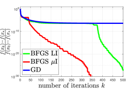
(a) $d=40$, $\kappa=10^{3}$.

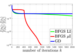
(b) $d=400$, $\kappa=10^{3}$.

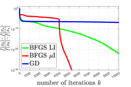
(c) $d=4000$, $\kappa=10^{3}$.

Figure 1: Convergence rates of BFGS with $B_{0}=LI$, $B_{0}=\mu I$ and gradient descent for solving the hard cubic objective function when condition number is fixed and dimension is modified.

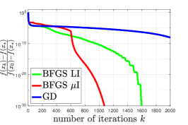
(a) $d=600$, $\kappa=10$.

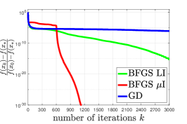
(b) $d=600$, $\kappa=10^{2}$.

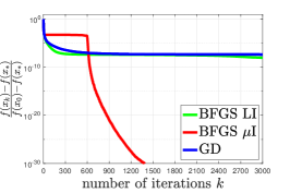
(c) $d=600$, $\kappa=10^{3}$.

Figure 2: Convergence rates of BFGS with $B_{0}=LI$, $B_{0}=\mu I$ and gradient descent for solving the hard cubic objective function when condition number is changing and dimension is fixed.

Several observations are in order. First, BFGS with $B_{0}=LI$ initially converges faster than BFGS with $B_{0}=\mu I$ in most plots, aligning with our theoretical findings that the linear convergence rate of BFGS with $B_{0}=LI$ surpasses that of $B_{0}=\mu I$.

Second, the transition to superlinear convergence for BFGS with $B_{0}=\mu I$ typically occurs around $k\approx d$, as predicted by our theoretical analysis. Interestingly, this transition does not always coincide with the iterates approaching the solution’s local neighborhood; in many cases, it occurs for BFGS with $B_{0}=\mu I$ even when its error is larger than that of gradient descent.

Third, although BFGS with $B_{0}=LI$ initially converges faster, its transition to superlinear convergence consistently occurs later than for $B_{0}=\mu I$. Notably, for a fixed dimension $d=600$, the transition to superlinear convergence for $B_{0}=LI$ occurs increasingly later as the problem condition number rises, an effect not observed for $B_{0}=\mu I$. This phenomenon indicates that the superlinear rate for $B_{0}=LI$ is more sensitive to the condition number $\kappa$, which corroborates our theory that the number of iterations required for superlinear convergence is $\mathcal{O}(d\kappa)$ for $B_{0}=LI$ and is improved to $\mathcal{O}(d\log{\kappa})$ for $B_{0}=\mu I$.

These findings align with our theoretical observations on the trade-off between global linear and superlinear convergence rates for different initial Hessian approximation matrices, as discussed in Sections 4 and 5.

8 Conclusion

In this paper, we proved explicit global linear and superlinear convergence rates for the BFGS method implemented with the exact line search scheme. Our results hold for any initial point $x_{0}$ and any initial Hessian approximation matrix $B_{0}\in\mathbb{S}_{++}^{d}$. We proved a global convergence rate of $\bigl{(}1-e^{-\frac{\Psi(\bar{B}_{0})}{k}}\frac{2}{\kappa\min\{2(1+C_{0}),1+\sqrt{\kappa}\}}\bigr{)}^{k}$, where $\bar{B}_{0}=B_{0}/L$ and $\Psi(\cdot)$ is defined in (18). This implies a linear rate of $(1-\frac{2}{\kappa\min\{2(1+C_{0}),1+\sqrt{\kappa}\}})^{k}$ when $k\geq\Psi(\bar{B}_{0})$. Moreover, we proved that the linear rate is improved to $(1-\frac{1}{3\kappa})^{k}$ after $\mathcal{O}((1+C_{0})\Psi(\bar{B}_{0})+C_{0}\kappa\min\{1+C_{0},\sqrt{\kappa}\})$ iterations. Finally, we proved a superlinear convergence rate of $\mathcal{O}(\frac{\Psi(\tilde{B}_{0})+C_{0}\Psi(\bar{B}_{0})+C_{0}\kappa\min\{1+C_{0},\sqrt{\kappa}\}}{k})^{k}$, where $\tilde{B}_{0}=\nabla^{2}f(x_{*})^{-\frac{1}{2}}B_{0}\nabla^{2}f(x_{*})^{-\frac{1}{2}}$.

We further showed that for the specific choice of $B_{0}=LI$, BFGS achieves a global linear convergence rate of $\mathcal{O}(1-\frac{1}{\kappa\min\{1+C_{0},\sqrt{\kappa}\}})^{k}$ from the first iteration, a improved linear rate of $(1-\frac{1}{3\kappa})^{k}$ after $\mathcal{O}(C_{0}\kappa\min\{1+C_{0},\sqrt{\kappa}\})$ iterations, and a superlinear convergence rate of $\mathcal{O}(\frac{d\kappa+C_{0}\kappa\min\{1+C_{0},\sqrt{\kappa}\}}{k})^{k}$. Moreover, for $B_{0}=\mu I$, BFGS achieves a global linear rate of $\mathcal{O}(1-\frac{1}{\kappa\min\{1+C_{0},\sqrt{\kappa}\}})^{k}$ after $\mathcal{O}(d\log{\kappa})$ iterations, a improved linear rate of $\mathcal{O}((1-\frac{1}{\kappa})^{k})$ after $\mathcal{O}(d\log{\kappa}+C_{0}\kappa\min\{1+C_{0},\sqrt{\kappa}\})$ iterations, and a superlinear rate of $\mathcal{O}(\frac{(1+C_{0})d\log{\kappa}+C_{0}\kappa\min\{1+C_{0},\sqrt{\kappa}\}}{k})^{k}$.

Appendix

Appendix A Proof of Proposition 2

First, we show that

$$\mathbf{Tr}(\hat{B}_{k+1}) =\mathbf{Tr}(\hat{B}_{k})-\frac{\|\hat{B}_{k}\hat{s}_{k}\|^{2}}{\hat{s}_{k}^{\top}\hat{B}_{k}\hat{s}_{k}}+\frac{\|\hat{y}_{k}\|^{2}}{\hat{s}_{k}^{\top}\hat{y}_{k}},$$ (66)

$$\mathbf{Det}(\hat{B}_{k+1}) =\mathbf{Det}(\hat{B}_{k})\frac{\hat{s}_{k}^{\top}\hat{y}_{k}}{\hat{s}_{k}^{\top}\hat{B}_{k}\hat{s}_{k}}.$$ (67)

Taking the trace on both sides of the equation (12) and using the fact that $\mathbf{Tr}(ab^{\top})=a^{\top}b$ for any vector $a$ and $b$, we obtain the equality in (66). Please check Lemma 6.2 of [RN21b] for the proof of (67). Take the logarithm on both sides of the above equation, we obtain that

$$\log{\frac{\hat{s}_{k}^{\top}\hat{y}_{k}}{\hat{s}_{k}^{\top}\hat{B}_{k}\hat{s}_{k}}}=\log{\mathbf{Det}(\hat{B}_{k+1})}-\log{\mathbf{Det}(\hat{B}_{k})}.$$

Recall that $\hat{m}_{k}=\frac{\hat{y}_{k}^{\top}\hat{s}_{k}}{\|\hat{s}_{k}\|^{2}}$ and $\cos(\hat{\theta}_{k})=-\hat{g}_{k}^{\top}\hat{s}_{k}/(\|\hat{g}_{k}\|\|\hat{s}_{k}\|)$. Since $\hat{B}_{k}\hat{s}_{k}=-\eta_{k}\hat{g}_{k}$, we also have $\cos(\hat{\theta}_{k})=\hat{s}_{k}^{\top}\hat{B}_{k}\hat{s}_{k}/(\|\hat{B}_{k}\hat{s}_{k}\|\|\hat{s}_{k}\|)$. Hence, we can write

$$\frac{\hat{s}_{k}^{\top}\hat{y}_{k}}{\hat{s}_{k}^{\top}\hat{B}_{k}\hat{s}_{k}}=\frac{\|\hat{B}_{k}\hat{s}_{k}\|^{2}\|\hat{s}_{k}\|^{2}}{(\hat{s}_{k}^{\top}\hat{B}_{k}\hat{s}_{k})^{2}}\frac{\hat{s}_{k}^{\top}\hat{y}_{k}}{\|\hat{s}_{k}\|^{2}}\frac{\hat{s}_{k}^{\top}\hat{B}_{k}\hat{s}_{k}}{\|\hat{B}_{k}\hat{s}_{k}\|^{2}}=\frac{\hat{m}_{k}}{\cos^{2}(\hat{\theta}_{k})}\frac{\hat{s}_{k}^{\top}\hat{B}_{k}\hat{s}_{k}}{\|\hat{B}_{k}\hat{s}_{k}\|^{2}}.$$

Thus, we obtain that

$$\Psi(\hat{B}_{k+1})-\Psi(\hat{B}_{k}) =\mathbf{Tr}(\hat{B}_{k+1})-\mathbf{Tr}(\hat{B}_{k})+\log\mathbf{Det}(\hat{B}_{k})-\log{\mathbf{Det}(\hat{B}_{k+1})}$$

$$=\frac{\|\hat{y}_{k}\|^{2}}{\hat{s}_{k}^{\top}\hat{y}_{k}}-\frac{\|\hat{B}_{k}\hat{s}_{k}\|^{2}}{\hat{s}_{k}^{\top}\hat{B}_{k}\hat{s}_{k}}-\log{\frac{\hat{s}_{k}^{\top}\hat{y}_{k}}{\hat{s}_{k}^{\top}\hat{B}_{k}\hat{s}_{k}}}$$

$$=\frac{\|\hat{y}_{k}\|^{2}}{\hat{s}_{k}^{\top}\hat{y}_{k}}-1+\log\frac{\cos^{2}\hat{\theta}_{k}}{\hat{m}_{k}}-\left(\frac{\|\hat{B}_{k}\hat{s}_{k}\|^{2}}{\hat{s}_{k}^{\top}\hat{B}_{k}\hat{s}_{k}}-\log\frac{\|\hat{B}_{k}\hat{s}_{k}\|^{2}}{\hat{s}_{k}^{\top}\hat{B}_{k}\hat{s}_{k}}+1\right)$$

$$\leq\frac{\|\hat{y}_{k}\|^{2}}{\hat{s}_{k}^{\top}\hat{y}_{k}}-1+\log\frac{\cos^{2}\hat{\theta}_{k}}{\hat{m}_{k}}.$$

where the last inequality holds since $x-\log x+1\geq 0$ for any $x>0$. Hence (19) follows from the above inequality. Finally, the result in (20) follows from summing both sides of (19) from $i=0$ to $k-1$, i.e.,

$$\sum_{i=0}^{k-1}\Psi(\hat{B}_{i+1})\leq\sum_{i=0}^{k-1}\Psi(\hat{B}_{i})+\sum_{i=0}^{k-1}\left(\frac{\|\hat{y}_{i}\|^{2}}{\hat{s}_{i}^{\top}\hat{y}_{i}}-1\right)+\sum_{i=0}^{k-1}\log\frac{\cos^{2}\hat{\theta}_{i}}{\hat{m}_{i}},$$

$$\Psi(\hat{B}_{k})\leq\Psi(\hat{B}_{0})+\sum_{i=0}^{k-1}\left(\frac{\|\hat{y}_{i}\|^{2}}{\hat{s}_{i}^{\top}\hat{y}_{i}}-1\right)+\sum_{i=0}^{k-1}\log\frac{\cos^{2}\hat{\theta}_{i}}{\hat{m}_{i}},$$

$$\sum_{i=0}^{k-1}\log{\frac{\cos^{2}(\hat{\theta}_{i})}{\hat{m}_{i}}}\geq\Psi(\hat{B}_{k})-\Psi(\hat{B}_{0})+\sum_{i=0}^{k-1}\left(1-\frac{\|\hat{y}_{i}\|^{2}}{\hat{s}_{i}^{\top}\hat{y}_{i}}\right)\geq-\Psi(\hat{B}_{0})+\sum_{i=0}^{k-1}\left(1-\frac{\|\hat{y}_{i}\|^{2}}{\hat{s}_{i}^{\top}\hat{y}_{i}}\right),$$

where the last inequality holds since $\Psi(\hat{B}_{k})\geq 0$ for any $k\geq 0$.

Appendix B Proof of Lemma 2

1. Recall that $J_{k}=\int_{0}^{1}\nabla^{2}{f(x_{k}+\tau(x_{k+1}-x_{k}))}d\tau$. Using the triangle inequality, we have

   $$\|\nabla^{2}{f(x_{*})}-J_{k}\| =\left\|\int_{0}^{1}\!\!\left(\nabla^{2}{f(x_{*})}-\nabla^{2}{f(x_{k}+\tau(x_{k+1}-x_{k}))}\right)d\tau\right\|$$

   $$\leq\int_{0}^{1}\|\nabla^{2}{f(x_{*})}-\nabla^{2}{f(x_{k}+\tau(x_{k+1}-x_{k}))}\|d\tau.$$

   Moreover, it follows from Assumption 3 that $\|\nabla^{2}{f(x_{*})}-\nabla^{2}{f(x_{k}+\tau(x_{k+1}-x_{k}))}\|\leq M\|(1-\tau)(x_{*}-x_{k})+\tau(x_{*}-x_{k+1})\|$ for any $\tau\in[0,1]$. Thus, we can further apply the triangle inequality to obtain

   $$\|\nabla^{2}{f(x_{*})}-J_{k}\| \leq\int_{0}^{1}M\|(1-\tau)(x_{*}-x_{k})+\tau(x_{*}-x_{k+1})\|d\tau$$

   $$\leq M\|x_{k}-x_{*}\|\int_{0}^{1}(1-\tau)d\tau+M\|x_{k+1}-x_{*}\|\int_{0}^{1}\tau d\tau$$

   $$=\frac{M}{2}(\|x_{k}-x_{*}\|+\|x_{k+1}-x_{*}\|).$$

   Since $f$ is strongly convex, by Assumption 1 and $f(x_{k+1})\leq f(x_{k})$, we have $\frac{\mu}{2}\|x_{k}-x_{*}\|^{2}\leq f(x_{k})-f(x_{*})$, which implies that $\|x_{k}-x_{*}\|\leq\sqrt{2(f(x_{k})-f(x_{*}))/\mu}$. Similarly, since $f(x_{k+1})\leq f(x_{k})$, it also holds that $\|x_{k+1}-x_{*}\|\leq\sqrt{2(f(x_{k+1})-f(x_{*}))/\mu}\leq\sqrt{2(f(x_{k})-f(x_{*}))/\mu}$. Hence, we obtain

   $$\|\nabla^{2}{f(x_{*})}-J_{k}\|\leq\frac{M}{\sqrt{\mu}}\sqrt{2(f(x_{k})-f(x_{*}))}$$ (68)

   Moreover, notice that by Assumption 1, we also have $J_{k}\succeq\mu I$ and $\nabla^{2}f(x_{*})\succeq\mu I$. Hence, (68) implies that

   $$\nabla^{2}{f(x_{*})}-J_{k} \preceq\|\nabla^{2}{f(x_{*})}-J_{k}\|I\preceq\frac{M}{\mu^{\frac{3}{2}}}\sqrt{2(f(x_{k})-f(x_{*}))}J_{k}=C_{k}J_{k},$$

   $$J_{k}-\nabla^{2}{f(x_{*})} \preceq\|J_{k}-\nabla^{2}{f(x_{*})}\|I\preceq\frac{M}{\mu^{\frac{3}{2}}}\sqrt{2(f(x_{k})-f(x_{*}))}\nabla^{2}{f(x_{*})}=C_{k}\nabla^{2}{f(x_{*})}.$$

   where we used the definition of $C_{k}$ in (23). By rearranging the terms, we obtain (24).

2. Recall that $G_{k}=\int_{0}^{1}\nabla^{2}{f(x_{k}+\tau(x_{*}-x_{k}))}d\tau$. Similar to the arguments in (a), we have

   $$\begin{split}\left\|\nabla^{2}{f(x_{*})}-G_{k}\right\|&=\left\|\int_{0}^{1}\left(\nabla^{2}{f(x_{*})}-\nabla^{2}{f(x_{k}+\tau(x_{*}-x_{k}))}\right)d\tau\right\|\\ &\leq\int_{0}^{1}\|\nabla^{2}{f(x_{*})}-\nabla^{2}{f(x_{k}+\tau(x_{*}-x_{k}))}\|d\tau\\ &\leq M\int_{0}^{1}\|(1-\tau)(x_{*}-x_{k})\|d\tau=M\|x_{k}-x_{*}\|\int_{0}^{1}(1-\tau)d\tau\\ &=\frac{M}{2}\|x_{k}-x_{*}\|\leq\frac{M}{\sqrt{\mu}}\sqrt{2(f(x_{k})-f(x_{*}))}.\end{split}$$ (69)

   Moreover, notice that by Assumption 1 we also have $G_{k}\succeq\mu I$ and $\nabla^{2}f(x_{*})\succeq\mu I$. The rest follows similarly as in the proof of (a) and we prove (25).

3. Recall that $J_{k}=\int_{0}^{1}\nabla^{2}{f(x_{k}+\hat{\tau}(x_{k+1}-x_{k}))}d\tau$. For any $\hat{\tau}\in[0,1]$, we have

   $$\begin{split}&\phantom{{}={}}\left\|\nabla^{2}{f(x_{k}+\hat{\tau}(x_{k+1}-x_{k}))}-J_{k}\right\|\\ &=\left\|\int_{0}^{1}\left(\nabla^{2}{f(x_{k}+\hat{\tau}(x_{k+1}-x_{k}))}-\nabla^{2}{f(x_{k}+\tau(x_{k+1}-x_{k}))}\right)d\tau\right\|\\ &\leq\int_{0}^{1}\left\|\nabla^{2}{f(x_{k}+\hat{\tau}(x_{k+1}-x_{k}))}-\nabla^{2}{f(x_{k}+\tau(x_{k+1}-x_{k}))}\right\|d\tau\\ &\leq\int_{0}^{1}M|\hat{\tau}-\tau|\|x_{k+1}-x_{k}\|d\tau\leq\frac{1}{2}M\|x_{k+1}-x_{k}\|.\end{split}$$ (70)

   Moreover, by using the triangle inequality, we have $\|x_{k+1}-x_{k}\|\leq\|x_{k+1}-x_{*}\|+\|x_{k}-x_{*}\|\leq\sqrt{\frac{2}{\mu}(f(x_{k+1})-f(x_{*}))}+\sqrt{\frac{2}{\mu}(f(x_{k})-f(x_{*}))}\leq 2\sqrt{\frac{2}{\mu}(f(x_{k})-f(x_{*}))}$. Combining this with (70), we obtain that

   $$\left\|\nabla^{2}{f(x_{k}+\hat{\tau}(x_{k+1}-x_{k}))}-J_{k}\right\|\leq\frac{M}{\sqrt{\mu}}\sqrt{2(f(x_{k})-f(x_{*}))}.$$

   Moreover, notice that by Assumption 1, we also have $\nabla^{2}{f(x_{k}+\hat{\tau}(x_{k+1}-x_{k}))}\succeq\mu I$ and $J_{k}\succeq\mu I$. The rest follows similarly as in the proof of (a) and we prove (26).

4. Recall that $G_{k}=\int_{0}^{1}\nabla^{2}{f(x_{k}+\tau(x_{*}-x_{k}))}d\tau$. For any $\tilde{\tau}\in[0,1]$, we have

   $$\begin{split}&\phantom{{}={}}\left\|\nabla^{2}{f(x_{k}+\tilde{\tau}(x_{*}-x_{k}))}-G_{k}\right\|\\ &=\left\|\int_{0}^{1}\left(\nabla^{2}{f(x_{k}+\tilde{\tau}(x_{*}-x_{k}))}-\nabla^{2}{f(x_{k}+\tau(x_{*}-x_{k}))}\right)d\tau\right\|\\ &\leq\int_{0}^{1}\left\|\nabla^{2}{f(x_{k}+\tilde{\tau}(x_{*}-x_{k}))}-\nabla^{2}{f(x_{k}+\tau(x_{*}-x_{k}))}\right\|d\tau\\ &\leq\int_{0}^{1}M|\tilde{\tau}-\tau|\|x_{k}-x_{*}\|d\tau\leq\frac{1}{2}M\|x_{k}-x_{*}\|\leq\frac{M}{\sqrt{\mu}}\sqrt{2(f(x_{k})-f(x_{*}))}.\end{split}$$ (71)

   Moreover, notice that by Assumption 1, we also have $\nabla^{2}{f(x_{k}+\tilde{\tau}(x_{*}-x_{k}))}\succeq\mu I$ and $G_{k}\succeq\mu I$. The rest follows similarly as in the proof of (a) and we prove (27).

References

• [Al-98] Mehiddin Al-Baali “Global and superlinear convergence of a restricted class of self-scaling methods with inexact line searches, for convex functions” In Computational Optimization and Applications 9.2 Springer, 1998, pp. 191–203
• [BV04] Stephen Boyd and Lieven Vandenberghe “Convex Optimization” New York, NY, USA: Cambridge University Press, 2004
• [Bro65] Charles G Broyden “A class of methods for solving nonlinear simultaneous equations” In Mathematics of computation 19.92 JSTOR, 1965, pp. 577–593
• [Bro67] Charles G Broyden “Quasi-Newton methods and their application to function minimisation” In Mathematics of Computation 21.99, 1967, pp. 368–381
• [Bro70] Charles G Broyden “The convergence of single-rank quasi-Newton methods” In Mathematics of Computation 24.110, 1970, pp. 365–382
• [BDM73] Charles George Broyden, John E Dennis Jr and Jorge J Moré “On the local and superlinear convergence of quasi-Newton methods” In IMA Journal of Applied Mathematics 12.3 Oxford University Press, 1973, pp. 223–245
• [BKS96] Richard H Byrd, Humaid Fayez Khalfan and Robert B Schnabel “Analysis of a symmetric rank-one trust region method” In SIAM Journal on Optimization 6.4 SIAM, 1996, pp. 1025–1039
• [BNY87] Richard H Byrd, Jorge Nocedal and Y. Yuan “Global convergence of a class of quasi-Newton methods on convex problems” In SIAM Journal on Numerical Analysis 24.5 SIAM, 1987, pp. 1171–1190
• [BN89] Richard H. Byrd and Jorge Nocedal “A Tool for the Analysis of Quasi-Newton Methods with Application to Unconstrained Minimization” In SIAM Journal on Numerical Analysis, Vol. 26, No. 3, 1989
• [CGT91] Andrew R. Conn, Nicholas I.. Gould and Ph L Toint “Convergence of quasi-Newton matrices generated by the symmetric rank one update” In Mathematical programming 50.1-3 Springer, 1991, pp. 177–195
• [Dav59] WC Davidon “VARIABLE METRIC METHOD FOR MINIMIZATION”, 1959
• [DMT89] JE Dennis, Héctor J Martinez and Richard A Tapia “Convergence theory for the structured BFGS secant method with an application to nonlinear least squares” In Journal of Optimization Theory and Applications 61.2 Springer, 1989, pp. 161–178
• [DM74] John E Dennis and Jorge J Moré “A characterization of superlinear convergence and its application to quasi-Newton methods” In Mathematics of computation 28.126, 1974, pp. 549–560
• [Dix72] L… Dixon “Quasi-newton algorithms generate identical points” In Mathematical Programming, Volume 2, pages 383–387, 1972
• [Fle70] Roger Fletcher “A new approach to variable metric algorithms” In The computer journal 13.3 Oxford University Press, 1970, pp. 317–322
• [Fle91] Roger Fletcher “A new variational result for quasi-Newton formulae” In SIAM Journal on Optimization 1.1 SIAM, 1991, pp. 18–21
• [FP63] Roger Fletcher and Michael JD Powell “A rapidly convergent descent method for minimization” In The computer journal 6.2 Oxford University Press, 1963, pp. 163–168
• [GG19] Wenbo Gao and Donald Goldfarb “Quasi-Newton methods: superlinear convergence without line searches for self-concordant functions” In Optimization Methods and Software 34.1 Taylor & Francis, 2019, pp. 194–217
• [Gol70] Donald Goldfarb “A family of variable-metric methods derived by variational means” In Mathematics of computation 24.109, 1970, pp. 23–26
• [Gre70] JOHN Greenstadt “Variations on variable-metric methods” In Mathematics of Computation 24.109, 1970, pp. 1–22
• [GT82] Andreas Griewank and Ph L Toint “Local convergence analysis for partitioned quasi-Newton updates” In Numerische Mathematik 39.3 Springer, 1982, pp. 429–448
• [JD23] Zhen-Yuan Ji and Yu-Hong Dai “Greedy PSB methods with explicit superlinear convergence” In Computational Optimization and Applications 85.3 Springer, 2023, pp. 753–786
• [JJM23] Ruichen Jiang, Qiujiang Jin and Aryan Mokhtari “Online Learning Guided Curvature Approximation: A Quasi-Newton Method with Global Non-Asymptotic Superlinear Convergence” In Proceedings of Thirty Sixth Conference on Learning Theory 195, 2023, pp. 1962–1992
• [JM23] Ruichen Jiang and Aryan Mokhtari “Accelerated quasi-newton proximal extragradient: Faster rate for smooth convex optimization” In Advances in Neural Information Processing Systems 36, 2023
• [JM20] Qiujiang Jin and Aryan Mokhtari “Non-asymptotic Superlinear Convergence of Standard Quasi-Newton Methods” In arXiv preprint arXiv:2003.13607, 2020
• [KBS93] H Fayez Khalfan, Richard H Byrd and Robert B Schnabel “A theoretical and experimental study of the symmetric rank-one update” In SIAM J. Optim. 3.1 SIAM, 1993, pp. 1–24
• [KTSK23] Vladimir Krutikov, Elena Tovbis, Predrag Stanimirović and Lev Kazakovtsev “On the Convergence Rate of Quasi-Newton Methods on Strongly Convex Functions with Lipschitz Gradient” In Mathematics 11.23 MDPI, 2023, pp. 4715
• [LF99] Donghui Li and Masao Fukushima “A Globally and Superlinearly Convergent Gauss–Newton-Based BFGS Method for Symmetric Nonlinear Equations” In SIAM Journal on Numerical Analysis 37.1 SIAM, 1999, pp. 152–172
• [LYZ22] Dachao Lin, Haishan Ye and Zhihua Zhang “Explicit convergence rates of greedy and random quasi-Newton methods” In Journal of Machine Learning Research 23.162, 2022, pp. 1–40
• [LYZ21] Dachao Lin, Haishan Ye and Zhihua Zhang “Greedy and random quasi-newton methods with faster explicit superlinear convergence” In Advances in Neural Information Processing Systems 34, 2021, pp. 6646–6657
• [LN89] Dong C Liu and Jorge Nocedal “On the limited memory BFGS method for large scale optimization” In Mathematical programming 45.1-3 Springer, 1989, pp. 503–528
• [MER18] Aryan Mokhtari, Mark Eisen and Alejandro Ribeiro “IQN: An incremental quasi-Newton method with local superlinear convergence rate” In SIAM Journal on Optimization 28.2 SIAM, 2018, pp. 1670–1698
• [MS10] Renato DC Monteiro and Benar Fux Svaiter “On the complexity of the hybrid proximal extragradient method for the iterates and the ergodic mean” In SIAM Journal on Optimization 20.6 SIAM, 2010, pp. 2755–2787
• [Noc80] Jorge Nocedal “Updating quasi-Newton matrices with limited storage” In Mathematics of computation 35.151, 1980, pp. 773–782
• [NW06] Jorge Nocedal and Stephen Wright “Numerical optimization” Springer Science Business Media, 2006
• [Pow76] Michael JD Powell “Some global convergence properties of a variable metric algorithm for minimization without exact line searches” In Nonlinear programming 9.1 American Mathematical Society, Providence, RI, USA, 1976, pp. 53–72
• [Pow71] MJD Powell “On the convergence of the variable metric algorithm” In IMA Journal of Applied Mathematics 7.1 Oxford University Press, 1971, pp. 21–36
• [RN21] Anton Rodomanov and Yurii Nesterov “Greedy Quasi-Newton Methods with Explicit Superlinear Convergence” In SIAM Journal on Optimization 31.1 Society for IndustrialApplied Mathematics, 2021, pp. 785–811
• [RN21a] Anton Rodomanov and Yurii Nesterov “New Results on Superlinear Convergence of Classical Quasi-Newton Methods” In Journal of Optimization Theory and Applications 188.3 Springer Nature BV, 2021, pp. 744–769
• [RN21b] Anton Rodomanov and Yurii Nesterov “Rates of Superlinear Convergence for Classical Quasi-Newton Methods” In Mathematical Programming Springer Berlin Heidelberg, 2021, pp. 1–32
• [Sha70] David F Shanno “Conditioning of quasi-Newton methods for function minimization” In Mathematics of computation 24.111, 1970, pp. 647–656
• [SS99] Mikhail V Solodov and Benar F Svaiter “A hybrid approximate extragradient–proximal point algorithm using the enlargement of a maximal monotone operator” In Set-Valued Analysis 7.4 Springer, 1999, pp. 323–345
• [THG17] Adrien B. Taylor, Julien M. Hendrickx and François Glineur “Smooth strongly convex interpolation and exact worst-case performance of first-order methods” In Mathematical Programming, Volume 161, pages 307–345, 2017
• [YOY07] Hiroshi Yabe, Hideho Ogasawara and Masayuki Yoshino “Local and superlinear convergence of quasi-Newton methods based on modified secant conditions” In Journal of Computational and Applied Mathematics 205.1 Elsevier, 2007, pp. 617–632
• [YLCZ23] Haishan Ye, Dachao Lin, Xiangyu Chang and Zhihua Zhang “Towards explicit superlinear convergence rate for SR1” In Mathematical Programming 199.1 Springer, 2023, pp. 1273–1303
• [YOR19] Arjevani1 Yossi, Shamir1 Ohad and Shiff Ron “Oracle complexity of second-order methods for smooth convex optimization” In Mathematical Programming, Series A (2019), 178:327–360, 2019
• [Yua91] Y. Yuan “A modified BFGS algorithm for unconstrained optimization” In IMA Journal of Numerical Analysis 11.3 Oxford University Press, 1991, pp. 325–332