Duality based error control for the Signorini problem

Abstract

In this paper we study the a posteriori bounds for a conforming piecewise linear finite element approximation of the Signorini problem. We prove new rigorous a posteriori estimates of residual type in $\operatorname{L}^{p}$, for $p\in(4,\infty)$ in two spatial dimensions. This new analysis treats the positive and negative parts of the discretisation error separately, requiring a novel sign- and bound-preserving interpolant, which is shown to have optimal approximation properties. The estimates rely on the sharp dual stability results on the problem in $\operatorname{W}^{2,(4-\varepsilon)/3}$ for any $\varepsilon\ll 1$. We summarise extensive numerical experiments aimed at testing the robustness of the estimator to validate the theory.

1 Introduction

Consider the open and convex set $\Omega\subset\mathbb{R}^{2}$ with a polygonal boundary $\partial\Omega$ and let $\bm{n}$ denote the outward pointing normal to $\partial\Omega$. This paper focuses on a variational inequality that emerges from the study of the following partial differential equation (PDE):

$$-\Delta u+u=f\text{ in }\Omega,$$ (1.1)

accompanied by the boundary conditions

$$u\geqslant 0,\quad\nabla u\cdot\bm{n}\geqslant 0,\quad u\nabla u\cdot\bm{n}=0\text{ on }\partial\Omega.$$ (1.2)

The specified conditions dictate that, for any segment $I\subset\partial\Omega$ where $u>0$, it follows that $\nabla u\cdot\bm{n}=0$ over $I$. This problem, along with its variants, finds applications in diverse areas such as elasto-plasticity, fluid flow in porous media [12], and finance [46]. Its transformation into a variational inequality has facilitated extensive analysis, notably in [31], which established the existence and uniqueness of solutions across a broad class of problems.

Significant progress has been made in deriving a priori error estimates for finite element approximations to variational inequalities, achieving optimal order in energy norms [13, 22, 33, 36], with notable advancements also reported in [26] and [34] for estimates in $\operatorname{L}^{\infty}(\Omega)$. Despite these developments, results in norms other than the energy norm remain relatively rare. For instance, [32] offers an a priori bound in $\operatorname{L}^{2}(\Omega)$, albeit in a single spatial dimension. The literature also documents bounds on trace norms along the Signorini boundary [38], with more recent studies, such as [16], extending bounds to several low-order global norms.

The theory of a posteriori error estimation for elliptic variational inequalities is significantly less well-developed than that for elliptic boundary value problems. Nonetheless, there have been several works on the Signorini problem as well as the related problem where the obstacle is interior to the domain rather than on the boundary. In [27], hierarchical estimates are used under the assumption that quadratic finite elements give better approximation than linears. Error estimates for variational inequalities with nontrivial boundary data are given in [30], estimates for an alternative form using Lagrange multipliers are given in [10, 45], with results for the discontinuous Galerkin method given in [44].

Rigorous a posteriori error bounds of residual type were derived for the variational inequality of the first kind for the Signorini problem in [15] for piecewise linear finite elements. Here, the authors give an upper bound in $\operatorname{H}^{1}(\Omega)$. Several other works have considered a posteriori control in energy norms, see [25]. Pointwise error control was established in [35]. Recent regularity results for the problem in which constraints only apply at the boundary [16] show that better rates can be achieved in this case, paving the way for a posteriori error estimates in lower order norms.

We remark that error estimates have been derived for this problem using the dual-weighted residual methodology (see for example [41]) to estimate the error in a target quantity. In particular, estimates follow for the $\operatorname{L}^{2}(\Omega)$-error, however the necessary stability of the dual problem enters as an assumption.

A priori and a posteriori error estimates in low order norms are established using duality arguments, and the resulting error bounds in for example $\operatorname{L}^{2}(\Omega)$ are standard in the literature for boundary value problems. The Aubin-Nitsche duality argument allows a priori and a posteriori bounds in non-energy norms, see [1] and the references therein. Application of this methodology has proved to be a challenge in the case of variational inequalities since the dual problem can lack the necessary regularity. Indeed, given smooth data, solutions of the Signorini problem are smooth away from the boundary, but suffer from singular points at the boundaries of the contact set, that is, the set of points at which the boundary changes type. In this work, using the ideas of an a priori argument recently given in [16], the approach taken in [32] in which different dual problems are considered for the positive and negative parts of the error is adapted for the a posteriori setting and combined with a two-sided approximation that takes the place of the usual Lagrange interpolant. The novelty in this work is that we are able to prove rigorous a posteriori error control in $\operatorname{L}^{p}(\Omega)$, for $p\in(4,\infty)$. The results in [16] suggest that the exponent $4$ is a critical value in the sense that piecewise linear finite element approximations achieve optimal a priori orders of convergence in $\operatorname{W}^{1,4-\varepsilon}(\Omega)$ for any $\varepsilon\ll 1$ but become increasingly suboptimal in $\operatorname{W}^{1,p}(\Omega)$ for $p>4$. Increasingly suboptimal convergence is also observed in $\operatorname{L}^{p}(\Omega)$ for $p>4$. We observe the same critical exponent for our a posteriori bounds, however the assumptions we require to derive them are weaker than the a priori setting. Furthermore, we are able to regain optimal convergence rates through adaptive refinement techniques.

The main aim of this paper to understand the theoretical framework in which duality arguments can be applied to obtain a posteriori error bounds in non-energy norms. To that end, we give a brief discussion of the underlying assumptions, and those used elsewhere in the literature. We defer technical discussions to the main body of the article, but give a brief overview here to put our results in context.

1. A regularity assumption on the structure of the contact set of the solution to the Signorini problem (known as Condition $(\mathbf{A})$) is required to prove regularity of the dual problem, and indeed such an assumption is commonplace in the literature [6, 7, 8, 16, 24, 28]. Condition $(\mathbf{A})$ excludes the possibility of a fractal contact set. Technical details will be given in Remark 2.4, but we note that this assumption has been proven to hold in some cases, with the general case still an open problem. All original results in this article depend upon Condition $(\mathbf{A})$, and it alone is sufficient to prove $h$-robust a posteriori error control in $\operatorname{L}^{p}(\Omega)$ for $p\in(4,\infty)$ on the positive part of the error (Theorem 3.12).

2. We utilise a dual problem to derive a bound for the negative part of the error that depends upon the discrete solution. We make an assumption on the structure of its contact set, denoted Condition $(\mathbf{a}_{h})$, which, to our knowledge, cannot be proven a priori, but can be verified a posteriori once the discrete solution is obtained. Using this, we have a posteriori error control on the negative part of the error for any discrete solution which satisfies Condition $(\mathbf{a}_{h})$ (Theorem 3.17). The bound has an $h$-dependent regularity constant which we are able to compute a posteriori (see Remark 3.16), and in numerical experiments remains small.

3. A strictly stronger assumption, known as Condition $(\mathbf{A}_{h})$ was used in [16] to obtain a priori error bounds in the $\operatorname{L}^{4}(\Omega)$ norm using duality methods, implies that the $h$-dependent constant mentioned above is uniformly bounded as $h\to 0$. Under this stronger assumption, the bound for the negative part of the error would therefore be $h$-robust.

The rest of the paper is set out as follows: In §2 we introduce notation, formalise the model problem and describe the finite element approximation. In §3 we state the key estimates and main results. In §4 we discuss bound-preserving interpolation from above and below. We introduce a new interpolant which is shown to preserve bilateral bounds have optimal approximation properties. The performance of our error estimates are then tested numerically in §5.

2 Problem setup

This section contains a summary of the problem at hand, as well as a brief review of the current state of the art for regularity of the variational inequality and its finite element approximation. We note that the article [16] considers the problem on the unit square. In this work, to make use of their results, we will do the same, but remark that arguments can be extended to convex polygonal domains.

In what follows, $\Omega\subseteq\mathbb{R}^{2}$ is assumed to be the unit square. Let $\omega$ be a measurable subset of the domain $\Omega$, and let $\operatorname{L}^{p}(\omega)$ denote the Lebesgue spaces of $p$-th power Lebesgue integrable functions over $\omega$ with corresponding norm $\left\|\cdot\right\|_{\operatorname{L}^{p}(\omega)}$. We denote $\left\langle\cdot,\cdot\right\rangle_{\omega}$ as the $\operatorname{L}^{2}$ inner product over $\omega$ and use the convention of dropping the subscript if $\omega=\Omega$. Finally, we let $\operatorname{W}^{k,p}(\omega)$ be the Sobolev space whose first $k$ weak derivatives are $\operatorname{L}^{p}(\omega)$ and let $\operatorname{H}^{k}(\omega):=\operatorname{W}^{k,2}(\omega)$ with corresponding norms $\left\|\cdot\right\|_{\operatorname{W}^{k,p}(\omega)}$ and $\left\|\cdot\right\|_{\operatorname{H}^{k}(\omega)}$ respectively. For a real-valued function $g$, we define $g_{+}=\max(g,0)$ and $g_{-}=\min(g,0)$.

We will also henceforth consistently use the notation that $p$ and $q$ denote Hölder conjugates satisfying

$$\frac{1}{p}+\frac{1}{q}=1,$$ (2.1)

with $p\in(4,\infty)$ and $q\in(1,\frac{4}{3})$.

We define the convex set of test and trial functions

$$\mathcal{K}=\{v\in H^{1}(\Omega):v\geqslant 0\text{ on }\partial\Omega\}\subset\operatorname{H}^{1}(\Omega)$$ (2.2)

that is appropriate to define the weak form of (1.1)–(1.2). It reads: let $f\in\operatorname{L}^{s}(\Omega)$, for $s\geqslant 2$ and find $u\in\mathcal{K}$ such that

$$a(u,v-u):=\left\langle\nabla u,\nabla v-\nabla u\right\rangle+\left\langle u,v-u\right\rangle\geqslant\left\langle f,v-u\right\rangle=:l(v-u)\quad\forall v\in\mathcal{K}.$$ (2.3)

This leads us to state some well known properties of the problem (1.1)–(1.2) as well as some new regularity results which require stronger assumptions on the problem data.

Proposition 2.1 (Regularity of the primal problem [23, Theorem 3.2.3.1]).

Given $f\in\operatorname{L}^{2}(\Omega)$ there exists a unique solution $u\in H^{2}(\Omega)$ to problem (2.3). Moreover

$$\left\|u\right\|_{\operatorname{H}^{2}(\Omega)}\leqslant C\left\|f\right\|_{\operatorname{L}^{2}(\Omega)}.$$ (2.4)

Remark 2.2.

There are variants of the Signorini problem for which this regularity result cannot be applied. For example, if the boundary also contains portions where Neumann and/or Dirichlet conditions are applied, then the boundary conditions can not be expressed in the correct form to apply Proposition 2.1. In this case we are not guaranteed $u\in\operatorname{H}^{2}(\Omega)$. Such problems do arise in practical applications. Indeed they are studied in [9, 4].

Definition 2.3 (Contact Set).

Let $u$ be the unique solution of problem (2.3). Since we have $u\in H^{2}(\Omega)$ from Proposition 2.1, $u$ has a continuous representative on $\overline{\Omega}$ which we may use to define the contact set

$$\mathcal{A}:=\{x\in\partial\Omega\mid u(\bm{x})=0\},$$

with $\mathring{\mathcal{A}}$ the relative interior of this set.

Remark 2.4 (Condition $(\mathbf{A})$).

Stronger regularity for the solution of (2.3) follows from an assumption referred to as Condition $(\mathbf{A})$ in [16], namely that the contact set, $\mathcal{A}$, consists of finitely many connected components and isolated points, and in particular the set of critical points (i.e. points contained in the boundary of the contact set) does not contain accumulation points.

This means that the relative interior, $\mathring{\mathcal{A}}$, is a union of open intervals in $\partial\Omega$. This is a common assumption in works relating to problems with a Signorini boundary, such as [6, 7, 8, 16, 24, 28], with a related assumption on the free boundary in a problem with an interior obstacle given in [13, 14]. We also mention [20], where a priori bounds in $\operatorname{H}^{1}(\Omega)$ are proved without this assumption, however their methods are not applicable to the analysis in this work.

Optimal error estimates in certain non-energy norms can be obtained for the Signorini problem if an appropriate dual problem can be defined which has sufficient regularity. Condition $(\mathbf{A})$ is a sufficient condition under which such a dual problem can be defined. It is not required for existence and uniqueness of the continuous problem, but is rather a regularity assumption. If Condition $(\mathbf{A})$ is not satisfied, optimal a priori estimates in the energy norm will still hold [20], but bounds in low order norms may be rendered suboptimal.

In order to violate this assumption, the solution to the Signorini problem would have to have infinitely many critical points. The boundary of the contact set would therefore contain accumulation points, meaning that approaching such a point, the solution along the boundary would switch from contact to non-contact infinitely many times and over arbitrarily small distances, see Figure 1.

We finally remark that this condition was recently shown to hold in [2] in polygonal domains in some cases, although the verification in the general setting remains a challenging open problem.

Figure 1: An illustration to show how the trace of a function which violates Condition $(\mathbf{A})$ might behave.

Proposition 2.5 (Improved Regularity of the Primal Problem [16, Theorem 2.3]).

Suppose that $u$ solves (2.3), and that Condition $(\mathbf{A})$ holds. If $f\in\operatorname{L}^{s}(\Omega)$ for $2<s<4$, then $u\in\operatorname{W}^{2,s}(\Omega)$. If $f\in\operatorname{L}^{s}(\Omega)$ for $4<s<\infty$ then $u$ admits a decomposition $u=u_{R}+u_{S}$ with $u_{R}\in\operatorname{W}^{2,s}(\Omega)$ and $u_{S}\in\operatorname{H}^{5/2-\epsilon}(\Omega)$.

Finite element discretisation

We consider $\mathscr{T}{}$ to be a conforming triangulation of $\Omega$, namely, $\mathscr{T}{}$ is a finite family of sets such that

1. $K\in\mathscr{T}{}$ implies $K$ is an open simplex or box,

2. for any $K,J\in\mathscr{T}{}$ we have that $\overline{K}\cap\overline{J}$ is a full lower-dimensional simplex (i.e., it is either $\emptyset$, a vertex, an edge or the whole of $\overline{K}$ and $\overline{J}$) of both $\overline{K}$ and $\overline{J}$ and

3. $\bigcup_{K\in\mathscr{T}{}}\overline{K}=\overline{\Omega}$.

We will make the assumption that the triangulation is shape-regular. Further, we define $h:\Omega\to\mathbb{R}$ to be the piecewise constant meshsize function of $\mathscr{T}{}$ given by

$$h(\bm{x}):=\max_{\overline{K}\ni\bm{x}}\text{diam}(K).$$ (2.5)

We let $\mathscr{E}{}$ be the skeleton (set of common interfaces) of the triangulation $\mathscr{T}{}$ and say $e\in\mathscr{E}$ if $e$ is on the interior of $\Omega$ and $e\in\partial\Omega$ if $e$ lies on the boundary $\partial\Omega$ and set $h_{e}$ to be the diameter of $e$. We let $\mathcal{R}^{1}(K)$ denote a space of piecewise linear (respectively bilinear) polynomials over a triangle (respectively quadrilateral), that is, $\mathcal{R}^{1}(K)\in\{\mathbb{P}^{1}(K)$, $\mathbb{Q}^{1}(K)\}$, and introduce the finite element space

$$\mathbb{V}:=\{\phi\in\operatorname{H}^{1}(\Omega):\phi|_{K}\in\mathcal{R}^{1}(K)\}$$ (2.6)

to be the usual space of continuous piecewise polynomial functions. We define the element patch of $K\in\mathscr{T}{}$ as

$$\widehat{K}:=\{J\in\mathscr{T}{}|\overline{J}\cap\overline{K}\neq\emptyset\}.$$

We also define a discrete analogue of $\mathcal{K}$ as

$$\mathcal{K}_{h}:=\{v\in\mathbb{V}:v\geqslant 0\text{ on }\partial\Omega\}=\mathcal{K}\cap\mathbb{V}\subset\operatorname{H}^{1}(\Omega).$$ (2.7)

We are now in a position to state the finite element approximation of (1.1)–(1.2) which is to find $U\in\mathcal{K}_{h}$ such that

$$a(U,\Phi-U)\geqslant l(\Phi-U)\quad\forall\Phi\in\mathcal{K}_{h},$$ (2.8)

Note that we restrict our attention to either piecewise linear finite element spaces on triangular meshes or piecewise bilinear spaces on quadrilateral meshes. For the sake of this work, we do not extend to higher degree polynomial approximation and consider only lowest order.

Proposition 2.6 (The discrete problem is well posed [29, Thm 2.1]).

For $f\in\operatorname{L}^{2}(\Omega)$ and all $h>0$ there exists a unique solution $U$ of (2.8).

Under slightly stronger assumptions, namely that $f$ is essentially bounded and a technical assumption on the discrete solution $U$, which we detail below, one can prove a priori estimates in $\operatorname{L}^{4}(\Omega)$ [16]. We note that this result is included for completeness, and that we do not make these additional assumptions.

Definition 2.7 (Discrete contact Set).

The discrete contact set is defined analogously to the contact set. With $U$ the solution to (2.8), we define

$$\mathcal{A}_{U}:=\{x\in\partial\Omega\mid U(\bm{x})=0\}.$$

Definition 2.8 (Condition $(\mathbf{A}_{h})$ [16]).

We say that Condition $(\mathbf{A}_{h})$ holds if there exist points $d_{i}$ lying on $\partial\Omega$ and numbers $\delta_{i}>0$ such that the intersections of the open balls $B_{\delta_{i}}(d_{i})$ and the boundary have non-zero distance from each other, and from the corners of the domain, such that the following holds for all sufficiently small $h>0$.

1. The sets $B_{\delta_{i}}(d_{i})\cap\partial\Omega$ cover the boundary of the discrete contact set, and such that each $B_{\delta_{i}}(d_{i})\cap\partial\Omega$ contains precisely one element of the boundary of the discrete contact set.

2. Every connected component of $\mathcal{A}_{U}$ has a non-empty interior.

We now summarise the range of a priori results and the main ideas used to derive them in [16] to illustrate the interplay of primal and dual regularity.

Remark 2.9 (A priori error bounds [16, Propositions 5.5 and 5.7]).

Let $u$ solve (2.3) for some $f\in\operatorname{L}^{p}(\Omega)$ with $p\in(4,\infty)$. Let $R:\operatorname{H}^{1}(\Omega)\to\mathbb{V}$ denote the Ritz projector and let $U\in\mathbb{V}$ be the solution of (2.8). Then for all $\varepsilon\in(0,1)$ there exists $C>0$ such that the superconvergence result

$$\left\|R(u)-U\right\|_{\operatorname{H}^{1}(\Omega)}\leqslant Ch^{\tfrac{3}{2}-\tfrac{2}{p}-\varepsilon}$$ (2.9)

holds. The authors additionally assume that $f\in\operatorname{L}^{\infty}(\Omega)$. With this assumption, using inverse estimates and choosing arbitrarily large $p$, the result (2.9) provides optimal control of $R(u)-U$ in the $\operatorname{W}^{1,s}(\Omega)$ norm for $s<4$, i.e.,

$$\left\|R(u)-U\right\|_{\operatorname{W}^{1,s}(\Omega)}\leqslant Ch.$$ (2.10)

Using an error bound in $\operatorname{W}^{1,\infty}(\Omega)$, which the authors also prove, a bound in $\operatorname{W}^{1,4}(\Omega)$ is obtained from equation (2.10) of optimal order up to arbitrarily small $\varepsilon$, namely

$$\left\|R(u)-U\right\|_{\operatorname{W}^{1,4}(\Omega)}\leqslant Ch^{1-\varepsilon}.$$ (2.11)

This result is combined with classical results on approximability of the Ritz projector to obtain

$$\left\|u-U\right\|_{\operatorname{W}^{1,4}(\Omega)}\leqslant Ch^{1-\varepsilon}.$$ (2.12)

The a priori result (2.12) is a key ingredient in an Aubin-Nitsche duality argument which uses a Hölder inequality to bound in the strongest norm possible for an appropriately defined dual solution, which does not have $\operatorname{H}^{2}(\Omega)$ regularity. The bound (2.12) is able to compensate for this and deliver optimal rates (up to an arbitrarily small positive number $\varepsilon$):

$$\left\|(u-U)_{+}\right\|_{\operatorname{L}^{4}(\Omega)}\leqslant Ch^{2-\varepsilon}.$$ (2.13)

If we additionally assume that Condition $(\mathbf{A}_{h})$ holds, then we also have

$$\left\|(u-U)_{-}\right\|_{\operatorname{L}^{4}(\Omega)}\leqslant Ch^{2-\varepsilon},$$ (2.14)

and therefore achieve full a priori error control in $\operatorname{L}^{4}(\Omega)$.

Note that convergence rates in $\operatorname{W}^{1,s}(\Omega)$ for $s>4$ are suboptimal, and that while the argument above can be modified to include stronger norms at a suboptimal rate, this suboptimality carries through to the $\operatorname{L}^{p}(\Omega)$ estimate, i.e.,

$$\left\|u-U\right\|_{\operatorname{L}^{p}(\Omega)}\leqslant Ch^{\tfrac{3}{2}+\tfrac{2}{p}-\varepsilon}.$$ (2.15)

3 A posteriori error control

In this section we state and prove the main result of this work, a rigorous a posteriori bound in $\operatorname{L}^{s}(\Omega)$ for $s>4$ for the problem (1.1). To begin we state some technical results.

Proposition 3.1 (Trace theorem in $\operatorname{L}^{s}$).

Let $v\in\operatorname{W}^{1,s}(K)$ with $s\in(1,\infty)$. Then, there exists a constant $C_{\text{tr}}$ depending only on $s$ and $K$ such that

$$\left\|v\right\|_{\operatorname{L}^{s}(\partial K)}\leqslant C_{\text{tr}}\!\left({h^{-\tfrac{1}{s}}\left\|v\right\|_{\operatorname{L}^{s}(K)}+h^{1-\tfrac{1}{s}}\left\|\nabla v\right\|_{\operatorname{L}^{s}(K)}}\right).$$ (3.1)

Definition 3.2 (Jump operator).

We define jump operators as $\left\llbracket v\right\rrbracket={{{v}|_{K_{1}}\bm{n}_{K_{1}}+{v}|_{K_{2}}}\bm{n}_{K_{2}}}$, $\left\llbracket\bm{v}\right\rrbracket={{\bm{v}|_{K_{1}}}}\cdot\bm{n}_{K_{1}}+{{\bm{v}|_{K_{2}}}}\cdot\bm{n}_{K_{2}}$.

Lemma 3.3 (Interpolation estimate).

Let $\mathcal{I}$ denote the piecewise linear Lagrange interpolator over $\mathscr{T}{}$. The following estimate holds for all elements $K\in\mathscr{T}{}$, faces $e\in\mathscr{E}$ and all functions $v\in\operatorname{W}^{2,s}(K)$ with $s>1$.

$$\max\!\left({h^{-2}\left\|v-\mathcal{I}v\right\|_{\operatorname{L}^{s}(K)},h^{-2+1/s}\left\|v-\mathcal{I}v\right\|_{\operatorname{L}^{s}(e)}}\right) \leqslant C\left\|v\right\|_{\operatorname{W}^{2,s}(\widehat{K})}.$$

3.1 Dual variational inequality

Motivated by the approach used in [32] to derive a priori $\operatorname{L}^{2}(\Omega)$ estimates, we define the following set

$$\mathcal{M}=\{v\in\operatorname{H}^{1}(\Omega)\mid v\leqslant 0\text{ on }\mathring{\mathcal{A}}\}.$$ (3.2)

For $p\in(4,\infty)$ consider the problem of finding $z\in\mathcal{M}$ such that

$$a(z,v-z)\geqslant\left\langle\max(0,u-U)^{p-1},v-z\right\rangle\quad\forall v\in\mathcal{M}.$$ (3.3)

Remark 3.4.

Observe that $z+u-U$ lies in $\mathcal{M}$, since by the definition of $\mathring{\mathcal{A}}$, $u$ vanishes there and $U\geqslant 0$ on $\partial\Omega$ by definition of $\mathcal{K}_{h}$, (2.7).

To derive a posteriori error bounds, we require results on the stability and regularity of the dual problem (3.3), which we will now quantify.

Before presenting the necessary results, we make the following definitions regarding the corners of the domain and the boundary conditions.

Definition 3.5.

We let $\{b_{1},...,b_{N_{p}}\}$ be the set of critical points that make up the boundary of $\mathring{\mathcal{A}}$ and the vertices of $\partial\Omega$. Note that under the assumption that Condition $(\mathbf{A})$ holds, this is a finite set consisting of the vertices of $\partial\Omega$ and the points at which there is a change in boundary condition. We let $\omega_{k}$ denote the angle at the boundary at $b_{k}$, that is, $\omega_{k}=\pi$ at a change of boundary conditions or $\omega_{k}=\tfrac{\pi}{2}$ at the corners of the domain, since the domain is the unit square. We will denote by $r_{k},\theta_{k}$ the polar coordinates centred at point $b_{k}$, $\zeta_{k}$ a smooth cut-off function identically equal to 1 in a neighbourhood of $b_{k}$, and $\phi_{k}=\phi_{k}(\theta_{k})$ a trigonometric function.

The functions described in Definition 3.5 are the key tools in quantifying the behaviour of the solution around the points $b_{k}$. The properties of the dual problem that we will need are summarised in the following lemma.

Proposition 3.6 (Properties of the dual problem [16]).

Let $u$ solve (2.3) for some $f\in\operatorname{L}^{2}(\Omega)$, and satisfy Condition $(\mathbf{A})$, and $U\in\mathbb{V}$ solve (2.8). Then the dual problem (3.3) is uniquely solvable in $\operatorname{H}^{1}(\Omega)$. In addition, we have $z\geqslant 0$ in $\Omega$ and $z=0$ on $\mathcal{A}$, and for any $p\in(4,\infty)$ and its conjugate $q=\tfrac{p}{p-1}$ there exists $C>0$ independent of $h$ such that the stability bound

$$\left\|z\right\|_{\operatorname{H}^{1}(\Omega)}\leqslant C\left\|\max(0,u-U)^{p-1}\right\|_{\operatorname{L}^{q}(\Omega)}$$ (3.4)

holds. Furthermore, we have the following regularity result in $\operatorname{W}^{2,q}(\Omega)$

$$\left\|z\right\|_{\operatorname{W}^{2,q}(\Omega)}\leqslant C\left\|\max(0,u-U)^{p-1}\right\|_{\operatorname{L}^{q}(\Omega)}.$$ (3.5)

Proof.

We first claim that $a(z_{+},z_{-})=0$. To see this, note that by definition we have $z=z_{+}+z_{-}$, and

$$a(z_{+},z_{-})=\int_{\Omega}\nabla z_{+}\cdot\nabla z_{-}+z_{+}z_{-}\mathop{}\!\mathrm{d}x.$$ (3.6)

It is clear that $z_{+}z_{-}\equiv 0$ since $z$ cannot be both positive and negative. Further, we can write $\Omega=\{x\in\Omega:z<0\}\cup\{x\in\Omega:z\geqslant 0\}$. Note that in each set, precisely at least one of $z_{+}$ and $z_{-}$ is identically the zero function, and therefore if the set has nonzero measure, its weak gradient must be zero there. Contributions to the integral (3.6) must therefore be zero and the claim is proved.

Since $z\in\mathcal{M}$, $z\leqslant 0$ on $\mathring{\mathcal{A}}$, its positive part must be zero there, and we may take $v=z_{+}$ as test function in (3.3), which yields

$$-\|z_{-}\|^{2}_{\operatorname{H}^{1}(\Omega)}=a(z,-z_{-})\geqslant\left\langle\max(0,u-U)^{p-1},-z_{-}\right\rangle.$$ (3.7)

In other words, since $\max(0,u-U)^{p-1}$ is non-negative and $z_{-}$ is non-positive,

$$0\leqslant\|z_{-}\|^{2}_{\operatorname{H}^{1}(\Omega)}\leqslant\left\langle\max(0,u-U)^{p-1},z_{-}\right\rangle\leqslant 0,$$ (3.8)

so that $z_{-}\equiv 0$, which proves that $z\geqslant 0$. This in turn gives $z=0$ on $\mathring{\mathcal{A}}$.

The bound (3.4) follows after noting that we can take $v=0$ in (3.3) to see

$$a(z,-z)\geqslant\left\langle\max(0,u-U)^{p-1},-z\right\rangle,$$ (3.9)

and $v=2z$ in (3.3), yielding

$$a(z,z)\geqslant\left\langle\max(0,u-U)^{p-1},z\right\rangle.$$ (3.10)

Therefore,

$$\begin{split}\left\|z\right\|^{2}_{\operatorname{H}^{1}(\Omega)}&=\left\langle\max(0,u-U)^{p-1},z\right\rangle\\ &\leqslant\left\|\max(0,u-U)^{p-1}\right\|_{\operatorname{L}^{q}(\Omega)}\left\|z\right\|_{\operatorname{L}^{p}(\Omega)}\\ &\leqslant C_{\text{Sob}}\left\|\max(0,u-U)^{p-1}\right\|_{\operatorname{L}^{q}(\Omega)}\left\|z\right\|_{\operatorname{H}^{1}(\Omega)},\end{split}$$

where we have used the embedding of $\operatorname{H}^{1}(\Omega)$ in $\operatorname{L}^{p}(\Omega)$ with embedding constant $C_{\text{Sob}}$. The result now follows after dividing by $\left\|z\right\|_{\operatorname{H}^{1}(\Omega)}$.

Now, $z$ is the weak solution of the boundary value problem

$$-\Delta z+z=\max(0,u-U)^{p-1},$$ (3.11)

with zero Dirichlet boundary condition on $\mathcal{A}$ and zero Neumann condition on the remainder of the boundary. The problem therefore fits into the framework of [23, Theorem 4.4.3.7], which allows us to quantify the regularity of $z$ to the following extent. With the notation of Definition 3.5, there exist unique real numbers $c_{k,m}$ such that

$$z-\sum_{\begin{subarray}{c}1\leqslant k\leqslant N_{p}\\ -2/q^{\prime}<\lambda_{k,m}<0\\ \lambda_{k,m}\neq-1\end{subarray}}c_{k,m}r^{-\lambda_{k,m}}\zeta_{k}\phi_{k}\in\operatorname{W}^{2,(4-\varepsilon)/(1-\varepsilon)}(\Omega),$$ (3.12)

where $q^{\prime}$ is the Hölder conjugate of $(4-\varepsilon)/(1-\varepsilon)$, $\lambda_{k,m}$ are eigenvalues of a Laplacian operator which depends upon $\omega_{k}$ (see [23, §4.4] for complete enumeration of the $\lambda_{k,m}$ in all cases). In our case where $\Omega$ is a convex polygonal domain, the regularity of $z$ is determined by the term in (3.12) with the lowest power of $r$, which is $r^{1/2}\zeta_{k}\phi_{k}$. The singularity of type $r^{1/2}$ occurs at points where the boundary condition changes (compare with [2, §3] on this point).

Now, we observe that $r^{1/2}\zeta_{k}\phi_{k}\in\operatorname{W}^{k,s}(\Omega)$ if and only if $k-\tfrac{2}{s}<\tfrac{1}{2}$. This gives a limit on the regularity of the second derivatives of $z$: $z\in\operatorname{W}^{2,s}(\Omega)$ only if $s<\tfrac{4}{3}$.

The proof of the stability bound in $\operatorname{W}^{2,q}(\Omega)$ is a technical argument that we will not reproduce here, but can be found in full in [16, Lemma 5.2]. ∎

Remark 3.7 (Smoothness of the dual problem).

It is important to note that the limit on regularity for the dual problem is imposed by the assumption of convexity of the domain and the nature of the boundary conditions, not the regularity of the problem data $f$. Indeed, the nonsingular part of $z$, that is, the expression in (3.12) possesses higher regularity depending on the problem data, but the regularity of the singular components of $u$ is limited by the geometry. For certain boundary conditions including the Signorini condition (1.2), $\operatorname{H}^{2}(\Omega)$-regularity follows from Proposition 2.1 which implies that the singular part of the solution vanishes. For the mixed boundary condition, this result does not apply, and the regularity is therefore constrained by the least regular of the components in (3.12).

Remark 3.8 (Choice of norm for a posteriori error estimation).

Proposition 3.6 also motivates a posteriori error estimation in $\operatorname{L}^{p}(\Omega)$ for $p>4$. We see that we can only apply a duality approach for $q<\tfrac{4}{3}$, with the Hölder conjugate of $\tfrac{4}{3}$ being $4$. Thus, $\operatorname{L}^{4+\varepsilon}(\Omega)$ for any $\varepsilon\ll 1$ is the weakest space in which estimates of the traditional residual form can be established. In particular, error estimates in $\operatorname{L}^{2}(\Omega)$ are not possible in this framework.

Proposition 3.9.

Let $u$ be the solution of (1.1)-(1.2) and suppose that $w\in\operatorname{H}^{1}(\Omega)$ has tr$(w)=0$ on $\mathring{\mathcal{A}}$. Then

$$a(u,w)=\left\langle f,w\right\rangle.$$ (3.13)

Proof.

In light of the structure of the contact set, described in Remark 2.4, it can be seen (see [16, thm 2.3]) that $u$ solves the boundary value problem

$$\begin{split}-\Delta u+u&=f\quad\text{in}\quad\Omega,\\ u&=0\quad\text{on}\quad\Gamma_{i},i=1,...,N,\\ \nabla u\cdot\bm{n}&=0\quad\text{on}\quad\Gamma_{i},i=N+1,...,N+M.\end{split}$$ (3.14)

Here, $\Gamma_{i}\subset\Omega$ are disjoint open line segments such that $\bigcup_{i=1}^{N+M}\bar{\Gamma}_{i}=\partial\Omega$, and such that there is a set $R$ of measure zero such that

$$\mathcal{A}=\bigcup_{i=1}^{N}\bar{\Gamma}_{i}\cup R.$$

The claim now follows immediately by testing (3.14) with $w$ and integrating by parts. ∎

3.2 Interpolation operator for bilateral approximation

We now discuss our requirements for a finite element interpolation operator, the construction of which is postponed to §4.

Assumption 3.10 (Bilateral optimal approximation).

We make the assumption that there exists an interpolation operator $\widehat{\Pi}:\operatorname{W}^{2,q}(\Omega)\to\mathbb{V}$ such that for any $w\in\operatorname{W}^{2,q}(\Omega)$, $q\in(1,\tfrac{4}{3})$, with $w\geqslant 0$,

$$0\leqslant\widehat{\Pi}(w)\leqslant w$$ (3.15)

and for any $K\in\mathscr{T}{}$

$$\left\|w-\widehat{\Pi}(w)\right\|_{\operatorname{L}^{q}(K)}\leqslant C_{b}h^{2}\left|w\right|_{\operatorname{W}^{2,q}(\widehat{{K}})}.$$ (3.16)

This interpolant is a crucial part of our a posteriori error analysis, as demonstrated by the following lemma, which allows us to introduce an interpolant into the error inequality for $(u-U)_{+}$. This is done by using the bilateral bounds (3.15) to determine the sign of $a\!\left({\widehat{\Pi}(z),u-U}\right)$.

Lemma 3.11.

Let $u$ be the solution of (1.1)-(1.2), $U$ be the finite element approximation satisfying (2.8), $z$ be the dual solution of (3.3) and $\widehat{\Pi}(z)$ be the bilateral approximation of $z$. Then

$$a\!\left({\widehat{\Pi}(z),u-U}\right)\leqslant 0.$$ (3.17)

Proof.

By equation (3.13) and since $0\leqslant\widehat{\Pi}(z)\leqslant z=0$ on $\mathring{\mathcal{A}}$, we have immediately that

$$a\!\left({u,\,\widehat{\Pi}(z)}\right)=\left\langle f,\widehat{\Pi}(z)\right\rangle.$$ (3.18)

Since $\widehat{\Pi}(z)\geqslant 0$, we may take $\Phi=U+\widehat{\Pi}(z)$ in (2.8), giving

$$a\!\left({U,\,-\widehat{\Pi}(z)}\right)\leqslant-\left\langle f,\widehat{\Pi}(z)\right\rangle.$$ (3.19)

The result then follows after combining (3.18) and (3.19). ∎

3.3 A posteriori error bounds

We are now ready to state and prove the main result of this article, a rigorous a posteriori bound in $\operatorname{L}^{p}(\Omega)$ for the problem (1.1) - (1.2). We prove this in two parts, bounding separately the quantities $\left\|(u-U)_{+}\right\|_{\operatorname{L}^{p}(\Omega)}$ and $\left\|(u-U)_{-}\right\|_{\operatorname{L}^{p}(\Omega)}$.

Theorem 3.12 (A posteriori upper bound for the positive part of the error).

Let $u$ solve problem (2.3) and $U$ be the finite element approximation. Then, for $p\in\left(4,\infty\right)$, $q=\tfrac{p}{p-1}$ its conjugate and $f\in\operatorname{L}^{p}(\Omega)$, we have

$$\left\|(u-U)_{+}\right\|_{\operatorname{L}^{p}(\Omega)}^{p}\leqslant\eta(U,f,h):=C\sum_{K\in\mathscr{T}{}}\left(\eta_{K}^{p}+\frac{1}{2}\eta_{J}^{p}\right),$$ (3.20)

where

$$\begin{split}\eta_{K}&=h^{2}\left\|-\Delta U+U-f\right\|_{\operatorname{L}^{p}(K)},\\ \eta_{J}&=h^{2-1/q}\left\|\left\llbracket\nabla U\right\rrbracket\right\|_{\operatorname{L}^{p}(\partial K)}.\end{split}$$ (3.21)

Proof.

We may select $v=z+u-U$ in (3.3); this function is shown to belong to $\mathcal{M}$ in Remark 3.4. We therefore have

$$\left\|(u-U)_{+}\right\|^{p}_{\operatorname{L}^{p}(\Omega)}\leqslant a(z,u-U).$$ (3.22)

We may use Lemma 3.11 to introduce $\widehat{\Pi}(z)$ as follows:

$$\left\|(u-U)_{+}\right\|^{p}_{\operatorname{L}^{p}(\Omega)}\leqslant a\!\left({z-\widehat{\Pi}(z),u-U}\right).$$ (3.23)

Since $z$ and $\widehat{\Pi}(z)$ both have zero trace on $\mathcal{A}$, we can use Proposition 3.9 to arrive at

$$\left\|(u-U)_{+}\right\|^{p}_{\operatorname{L}^{p}(\Omega)}\leqslant l\!\left({z-\widehat{\Pi}(z)}\right)-a\!\left({z-\widehat{\Pi}(z),U}\right).$$

The rest of the argument follows standard a posteriori techniques, to begin

$$\begin{split}l\!\left({z-\widehat{\Pi}(z)}\right)-a\!\left({U,z-\widehat{\Pi}(z)}\right)&=\int_{\Omega}f\!\left({z-\widehat{\Pi}(z)}\right)-\nabla U\cdot\!\left({\nabla z-\nabla\widehat{\Pi}(z)}\right)-U\!\left({z-\widehat{\Pi}(z)}\right)\mathop{}\!\mathrm{d}x\\ &=\int_{\Omega}\!\left({f+\Delta U-U}\right)\!\left({z-\widehat{\Pi}(z)}\right)\mathop{}\!\mathrm{d}x-\int_{\mathscr{E}\cup\partial\Omega}\left\llbracket\nabla U\right\rrbracket\!\left({z-\widehat{\Pi}(z)}\right)\mathop{}\!\mathrm{d}S\\ &=:R_{1}+R_{2}.\end{split}$$ (3.24)

Splitting the integral elementwise and making use of the Cauchy-Schwarz inequality, we see that

$$\begin{split}R_{1}&=\int_{\Omega}\!\left({f+\Delta U-U}\right)\!\left({z-\widehat{\Pi}(z)}\right)\mathop{}\!\mathrm{d}x\\ &\leqslant\sum_{K\in\mathscr{T}{}}\left\|h^{2}\!\left({f+\Delta U-U}\right)\right\|_{\operatorname{L}^{p}(K)}\left\|h^{-2}\!\left({z-\widehat{\Pi}(z)}\right)\right\|_{\operatorname{L}^{q}(K)}.\end{split}$$ (3.25)

Invoking the optimal approximation result of Assumption 3.10 (proven in Lemma 4.4), we obtain

$$R_{1}\leqslant C_{b}\sum_{K\in\mathscr{T}{}}\left\|h^{2}\!\left({f+\Delta U-U}\right)\right\|_{\operatorname{L}^{p}(K)}|z|_{\operatorname{W}^{2,q}(\widehat{K})}.$$ (3.26)

Similarly, we bound $R_{2}$,

$$\begin{split}R_{2}&=-\sum_{e\in\mathscr{E}\cup\partial\Omega}\int_{e}\left\llbracket\nabla U\right\rrbracket\!\left({z-\widehat{\Pi}(z)}\right)\\ &\leqslant\frac{1}{2}\sum_{K\in\mathscr{T}{}}\!\left({\sum_{e\in\partial K}\left\|h^{2-1/q}\left\llbracket\nabla U\right\rrbracket\right\|_{\operatorname{L}^{p}(e)}\left\|h^{-2+1/q}\!\left({z-\widehat{\Pi}(z)}\right)\right\|_{\operatorname{L}^{q}(e)}}\right).\end{split}$$ (3.27)

To bound this term we use split $z-\widehat{\Pi}(z)=(z-\mathcal{I}z)+(\mathcal{I}z-\widehat{\Pi}(z))$ and use the triangle inequality. We may then use approximation properties of the Lagrange interpolant on element boundaries, trace estimates (see Proposition 3.1), inverse estimates and Assumption 3.10 to finally arrive at

$$R_{2}\leqslant C_{b}C_{\text{tr}}(1+C_{\text{inv}})\frac{1}{2}\sum_{K\in\mathscr{T}{}}\left\|h^{2-1/q}\left\llbracket\nabla U\right\rrbracket\right\|_{\operatorname{L}^{p}(\partial K)}\left|z\right|_{\operatorname{W}^{2,q}(\widehat{K})},$$ (3.28)

where $C_{\text{inv}}$ is the constant from the inverse inequality. Collecting (3.26)–(3.28), we have

$$\left\|(u-U)_{+}\right\|^{p}_{\operatorname{L}^{p}(\Omega)}\leqslant l\!\left({z-\widehat{\Pi}(z)}\right)-a\!\left({U,z-\widehat{\Pi}(z)}\right)\leqslant C\sum_{K\in\mathscr{T}{}}\!\left({\eta_{K}+\frac{1}{2}\eta_{J}}\right)|z|_{\operatorname{W}^{2,q}(\widehat{K})}.$$ (3.29)

Hence, the result follows from a discrete Cauchy-Schwarz inequality and the regularity bound on $z$ given in equation (3.5), after noting that, since $1/p+1/q=1$,

$$\left\|(u-U)^{p-1}_{+}\right\|_{\operatorname{L}^{q}(\Omega)}=\left\|(u-U)_{+}\right\|^{p-1}_{\operatorname{L}^{p}(\Omega)}.$$

∎

We now prove that the negative part of the error also satisfies a bound of the form (3.20). Once again taking an analogous approach to that in [32], we define a second dual problem as follows: let $\bar{\mathcal{M}}=\{v\mid v\geqslant 0\text{ on }\mathcal{A}_{U}\}$. Find $\bar{z}\in\bar{\mathcal{M}}$ such that

$$a(\bar{z},v-\bar{z})\geqslant\left\langle-\max(0,U-u)^{p-1},v-\bar{z}\right\rangle\quad\forall v\in\bar{\mathcal{M}}.$$ (3.30)

Key properties follow in a manner analogous to Proposition 3.6, and are summarised in Proposition 3.15. This result relies on a mild assumption, a posteriori verifiable from the discrete solution $U$, which we detail below.

Definition 3.13 (Condition $(\mathbf{a}_{h})$).

For the finite element approximation $U$, we say Condition $(\mathbf{a}_{h})$ holds if there exist finitely many points $d_{i}$ lying on $\partial\Omega$ and numbers $\delta_{i}>0$ such that the intersections of the open balls $B_{\delta_{i}}(d_{i})$ and the boundary have non-zero distance from each other, and from the corners of the domain, and such that

1. The sets $B_{\delta_{i}}(d_{i})\cap\partial\Omega$ cover the boundary of the discrete contact set, and such that each $B_{\delta_{i}}(d_{i})\cap\partial\Omega$ contains precisely one element of the boundary of the discrete contact set.

2. Every connected component of $\mathcal{A}_{U}$ has a non-empty interior.

We now have three related conditions: Condition $(\mathbf{A})$, Condition $(\mathbf{A}_{h})$ and Condition $(\mathbf{a}_{h})$ The latter two conditions are not discrete analogues of the first; indeed any finite element function may only have a contact set with finitely many connected components. Rather they place some restrictions on the boundaries of discrete contact sets. We note that in the continuous case, the contact set is allowed to contain singletons, whereas this is not allowed for discrete solutions. In addition, Condition $(\mathbf{A}_{h})$ assumes topological stability of the discrete contact set as $h\to 0$.

Remark 3.14 (Verification of Condition $(\mathbf{a}_{h})$).

Notice that the Condition $(\mathbf{a}_{h})$ is strictly weaker than its a priori sibling Condition $(\mathbf{A}_{h})$ where in addition, the topology of the discrete contact set is assumed to be stable in the limit $h\to 0$. Condition $(\mathbf{a}_{h})$ ensures that the discrete contact set does not include isolated singletons, and that the boundary of the discrete contact set does not include any of the corners of the domain. This condition can be verified a posteriori from the discrete solution $U$ by examination of the boundary nodal values. For example, since $U$ is piecewise linear on the boundary, a boundary degree of freedom is a singleton component of $\mathcal{A}_{U}$ if and only if it is zero and its neighbouring boundary degrees of freedom are both non-zero. Likewise, a degree of freedom at a corner of the domain is in the boundary of $\mathcal{A}_{U}$ if it is zero and precisely one of its neighbours is non-zero. Thus, one can iterate over boundary degrees of freedom and if neither of these situations occur, then Condition $(\mathbf{a}_{h})$ holds for $U$.

We remark that this condition is only required to prove bounds on the negative part of the error. This is due to the different convex sets in which solutions are sought for the two dual problems. The set $\mathcal{M}$ is defined using the contact set of $u$, and is therefore $h$-independent, whereas the definition of $\bar{\mathcal{M}}$ involves the discrete contact set.

Proposition 3.15 (Properties of dual problem for the negative part of the error [16]).

Let $u$ solve (2.3) for some $f\in\operatorname{L}^{2}(\Omega)$, and $U\in\mathbb{V}$ solve (2.8), with $U$ satisfying Condition $(\mathbf{a}_{h})$. Then the dual problem (3.30) is uniquely solvable in $\operatorname{H}^{1}(\Omega)$. In addition we have $\bar{z}\leqslant 0$ in $\Omega$ and $\bar{z}=0$ on $\mathcal{A}_{U}$. For $p\in(4,\infty)$ and its conjugate $q=\tfrac{p}{p-1}$ there exists $C>0$ such that the stability bound

$$\left\|\bar{z}\right\|_{\operatorname{H}^{1}(\Omega)}\leqslant C\left\|\max(0,U-u)^{p-1}\right\|_{\operatorname{L}^{q}(\Omega)}$$ (3.31)

holds. In addition, we have the following regularity result

$$\left\|\bar{z}\right\|_{\operatorname{W}^{2,q}(\Omega)}\leqslant C\left\|\max(0,U-u)^{p-1}\right\|_{\operatorname{L}^{q}(\Omega)}.$$ (3.32)

Remark 3.16 (The constant in Proposition 3.15).

A closer examination of the proof of Proposition 3.15, given in [16, Lemma 5.6] reveals that the constant in Equation (3.32) hides a dependence on the number of boundary points of the contact set of the discrete solution. To better quantify this regularity constant, we give some details of the proof. For some $h$, under the given assumptions there are finitely many, $N_{h}$, say, critical points (i.e. the boundary points of $\mathcal{A}_{U}$). If $\psi_{i}$ is a smooth cut-off function that is identically 1 in a neighbourhood of the $i$th critical point for $i=1,...,d$ and $\psi_{0}=1-\sum_{i=1}^{N_{h}}\psi_{i}$, such that their supports are disjoint, then $\bar{z}$ admits a decomposition

$${\bar{z}=z_{0}+z_{1}+...+z_{N_{h}},}$$

where for each $i$ we have defined $z_{i}=\psi_{i}\bar{z}$. Each locally supported function is shown to satisfy a regularity bound

$${\left\|z_{i}\right\|_{\operatorname{W}^{2,q}(\Omega)}\leqslant C_{i}\left\|\max(0,U-u)^{p-1}\right\|_{\operatorname{L}^{q}(\Omega)}}$$

and therefore

$${\left\|\bar{z}\right\|_{\operatorname{W}^{2,q}(\Omega)}\leqslant\sum_{i}C_{i}\left\|\max(0,U-u)^{p-1}\right\|_{\operatorname{L}^{q}(\Omega)}\leqslant(N_{h}+1)C\left\|\max(0,U-u)^{p-1}\right\|_{\operatorname{L}^{q}(\Omega)},}$$

where $C$ is the maximum of the $C_{i}$.The quality of the upper bound therefore depends upon the behaviour of $N_{h}$ as $h\to 0$. Typically it is observed in numerical experiments that the number and location of critical points converge to their true values (see for example [16, 38] and §5). In [38, §7], the distance between a discrete critical point and its true location was always bounded from above by the mesh size.

If $N_{h}$ changes significantly under mesh refinement, as noted in Remark 3.14 once the finite element approximation is known we are able to determine the number of critical points by examining the boundary degrees of freedom (see Remark 3.14) so that if $N_{h}$ does increase, its expected increase in size can be quantified. If $N_{h}$ were to increase without limit, this would imply that discrete solutions can oscillate between contact and non-contact over arbitrarily small distances, behaviour that is not present at the continuous level in light of the assumed Condition $(\mathbf{A})$.The stronger Condition $(\mathbf{A}_{h})$ assumes that this number remains uniformly bounded as $h\to 0$. Under this assumption there exists a single constant such that the results of Proposition 3.15 are true for all sufficiently small $h$.

Since $\bar{z}\leqslant 0$, we may now once again use the two-sided approximation. Let $\widecheck{\Pi}(\bar{z})=-\widehat{\Pi}(-\bar{z})$. Then by Assumption 3.10 (proven in §4), $\widecheck{\Pi}(\bar{z})$ is a finite element function such that $\bar{z}\leqslant\widecheck{\Pi}(\bar{z})\leqslant 0$ with required local approximation properties.

Theorem 3.17 (A posteriori upper bound for the negative part of the error).

Let $u$ solve problem (2.3) and $U$ be the FE approximation, with $U$ satisfying Condition $(\mathbf{a}_{h})$. Then, for $p\in\left(4,\infty\right)$, $q=\tfrac{p}{p-1}$ its conjugate and $f\in\operatorname{L}^{p}(\Omega)$ we have

$$\left\|(u-U)_{-}\right\|_{\operatorname{L}^{p}(\Omega)}^{p}\leqslant\eta(U,f,h):=C\sum_{K\in\mathscr{T}{}}\left(\eta_{K}^{p}+\frac{1}{2}\eta_{J}^{p}\right),$$ (3.33)

where

$$\begin{split}\eta_{K}&=h^{2}\left\|-\Delta U+U-f\right\|_{\operatorname{L}^{p}(K)},\\ \eta_{J}&=h^{2-1/q}\left\|\left\llbracket\nabla U\right\rrbracket\right\|_{\operatorname{L}^{p}(\partial K)}.\end{split}$$ (3.34)

Proof.

We may immediately take $v=\bar{z}+u-U$ in the dual problem since $U=0$ and $u\geqslant 0$ on $\mathcal{A}_{U}$. We therefore have

$$\int_{\Omega}\max(0,U-u)^{p}=\left\|(u-U)_{-}\right\|^{p}_{\operatorname{L}^{p}(\Omega)}\leqslant a(u-U,\bar{z}).$$ (3.35)

Since we know that $U=0$ on $\mathcal{A}_{U}$ and non-negative on $\partial\Omega$, and since we also have $\bar{z}=0$ on $\mathcal{A}_{U}$ and non-positive on $\Omega$, we can choose sufficiently small $s>0$ so that $U\pm s\widecheck{\Pi}(\bar{z})\in\mathcal{K}_{h}$. Taking $\Phi=U\pm s\widecheck{\Pi}(\bar{z})$ as test functions in the discrete problem (2.8) gives

$$\begin{split}a\!\left({U,\widecheck{\Pi}(\bar{z})}\right)&\geqslant\left\langle f,\widecheck{\Pi}(\bar{z})\right\rangle,\\ a\!\left({U,-\widecheck{\Pi}(\bar{z})}\right)&\geqslant-\left\langle f,\widecheck{\Pi}(\bar{z})\right\rangle,\end{split}$$ (3.36)

and therefore we must have

$$a\!\left({U,\widecheck{\Pi}(\bar{z})}\right)=\left\langle f,\widecheck{\Pi}(\bar{z})\right\rangle.$$ (3.37)

Choosing $v=u-\widecheck{\Pi}(\bar{z})\in\mathcal{K}$ in (2.3) we also have

$$a\!\left({u,-\widecheck{\Pi}(\bar{z})}\right)\geqslant-\left\langle f,\widecheck{\Pi}(\bar{z})\right\rangle.$$ (3.38)

Together with (3.35), we have shown

$$\left\|(u-U)_{-}\right\|^{p}_{\operatorname{L}^{p}(\Omega)}\leqslant a\!\left({u-U,\bar{z}-\widecheck{\Pi}(\bar{z})}\right).$$ (3.39)

To introduce the problem data, $f$, of the primal problem, we choose $v=u+\widecheck{\Pi}(\bar{z})-\bar{z}$ as test function in (2.3). Since $\widecheck{\Pi}(\bar{z})$ lies between the (non-positive) $\bar{z}$ and zero, this function lies in $\mathcal{K}$, and we obtain

$$a\!\left({u,\widecheck{\Pi}(\bar{z})-\bar{z}}\right)\geqslant\left\langle f,\widecheck{\Pi}(\bar{z})-\bar{z}\right\rangle,$$ (3.40)

or, equivalently.

$$a\!\left({u,\bar{z}-\widecheck{\Pi}(\bar{z})}\right)\leqslant\left\langle f,\bar{z}-\widecheck{\Pi}(\bar{z})\right\rangle.$$ (3.41)

Inserting this in (3.39), we now have

$$\left\|(u-U)_{-}\right\|^{p}_{\operatorname{L}^{p}(\Omega)}\leqslant\left\langle f,\bar{z}-\widecheck{\Pi}(\bar{z})\right\rangle-a\!\left({U,\bar{z}-\widecheck{\Pi}(\bar{z})}\right).$$ (3.42)

The proof now proceeds exactly as in Theorem 3.12. ∎

4 Two-sided approximation

In this section we develop the bound preserving interpolant used to prove the a posteriori error bounds in §3. We construct an interpolant that is bounded from above by a particular function in §4.2. Then, in §4.3, we introduce a new interpolant that satisfies bilateral bounds and prove that it enjoys the same optimal approximation properties as the Lagrange interpolant.

Let $\{x_{i}\}_{i=1}^{N}$ denote the vertices of the triangulation $\mathscr{T}{}$ and let $\phi_{i}\in\mathbb{V}$ be the $i$-th canonical basis function, with $\phi_{i}(x_{j})=\delta_{ij}$ for $i,j=1,\dots,N$. Let

$$\widehat{x}_{j}:=\bigcup\{K\in\mathscr{T}{}:\text{supp}(\phi_{j})\cap K\neq\emptyset\}.$$ (4.1)

We also recall that $\mathcal{I}$ denotes the (piecewise linear) nodal Lagrange interpolation operator. Let $q\in(1,\tfrac{4}{3})$ and assume we have a function $0\leqslant z\in\operatorname{W}^{2,q}(\Omega)$. Then the aim of this section is to examine the question of existence of an interpolation operator $\widehat{\Pi}:\operatorname{W}^{2,q}(\Omega)\to\mathbb{V}$ satisfying both

$$\begin{split}0\leqslant\widehat{\Pi}(z)&\leqslant z\text{ and }\\ \left\|z-\widehat{\Pi}(z)\right\|_{\operatorname{L}^{q}(\Omega)}&\leqslant Ch^{2}\left\|z\right\|_{\operatorname{W}^{2,q}(\Omega)}.\end{split}$$ (4.2)

In other words, we wish to show that there exists a two-sided approximation that also has the optimal approximation properties enjoyed by the Lagrange interpolant (see Proposition 3.3). This form of approximation theory arises in many areas of finite element analysis. In particular, the optimal approximation of non-smooth functions is a non trivial task relying on local averaging, see Clément [17], later extended to zero boundary values in [37].

4.1 From below

In this section we discuss positivity preserving interpolation. We note that since we work in two spatial dimensions, and since $q\in(1,\tfrac{4}{3})$, point values are well defined in $\operatorname{W}^{2,q}(\Omega)$. In this case, one can simply consider the Lagrange interpolant, which has the properties

$$\mathcal{I}z\geqslant 0\text{ if }z\geqslant 0,$$ (4.3)

see Figure 2(a), as well as optimal approximation locally and globally:

$$\left\|z-\mathcal{I}z\right\|_{\operatorname{L}^{q}(\Omega)}\leqslant Ch^{2}\left\|z\right\|_{\operatorname{W}^{2,q}(\Omega)}.$$ (4.4)

(a) Approximation with the piecewise linear Lagrange interpolant, $\mathcal{I}(z)$. Notice it is positive. this text ensures the figure aligns properly. EVEN MORE HERE

(b) Approximation with a nonlinear interpolant $\Pi(z)$. Notice it is bounded above by the function, but is no longer bounded below by zero.

(c) Approximation with the modified bilateral approximation $\widehat{\Pi}(z)$. Notice that $0\leqslant\widehat{\Pi}(z)\leqslant z$. this text ensures the figure aligns properly.

Figure 2: An illustration of three piecewise linear operators, black, applied to the same function, blue, that satisfies $z>0$. The Lagrange interpolant, $\mathcal{I}(z)\geqslant 0$, the nonlinear interpolant $\Pi(z)\leqslant z$ and the bilateral approximation $0\leqslant\widehat{\Pi}(z)\leqslant z$.

If point values do not exist, the approximation is considerably more involved, although has been tackled in [15] where an interpolant is constructed through local mean-values of the function. It was shown in [15] that the constructed interpolant is $\operatorname{L}^{q}$-stable, second order accurate and linear. See also [42, 43] for related ideas using a nonlinear interpolation operator [18].

4.2 From above

In this section we examine the design of interpolants that are bounded from above by the function to be interpolated. This means that we seek an interpolation operator $\Pi$ that satisfies $\Pi(z)\leqslant z$. In this case we can see the Lagrange interpolant does not satisfy the requirements, see Figure 2(a). Indeed, any strictly convex function will see the Lagrange interpolant violate this bound. It can, however, be modified. Indeed, consider the function:

$$\Pi(z)(x)=\sum_{i=1}^{N}\!\left({\mathcal{I}z(x_{i})-\max_{y\in\widehat{x}_{i}}(\mathcal{I}(z)(y)-z(y))}\right)\phi_{i}(x)=:\mathcal{I}(z)(x)-R(x).$$ (4.5)

Lemma 4.1.

For $0\leqslant z\in\operatorname{W}^{2,q}(\Omega)$ the approximation $\Pi(z)$ defined in (4.5) satisfies

$$\Pi(z)\leqslant z\text{ in }\Omega.$$ (4.6)

Proof.

Note that by definition of $R$ we have

$$\Pi(z)=\mathcal{I}(z)-R\leqslant\mathcal{I}(z)-(\mathcal{I}(z)-z)=z.$$ (4.7)

∎

This is a nonlinear interpolant since for general $u,v\in\operatorname{W}^{2,q}(\Omega)$

$$\Pi(u+v)\neq\Pi(u)+\Pi(v).$$ (4.8)

This means we cannot directly apply Bramble-Hilbert to obtain optimal approximation under minimal regularity. Instead we must take a different approach.

Theorem 4.2 (Optimal approximation).

Suppose $z\in\operatorname{W}^{2,q}(\Omega)$, for $q\in(1,\tfrac{4}{3})$. Then there exists $C>0$ independent of $h$ such that for all elements $K\in\mathscr{T}{}$ the approximation $\Pi(z)$ defined through (4.5) satisfies

$$\left\|z-\Pi(z)\right\|_{\operatorname{L}^{q}(K)}\leqslant Ch^{2}\left|z\right|_{\operatorname{W}^{2,q}(\widehat{K})}.$$ (4.9)

Proof.

To begin, we note

$$\left\|z-\Pi(z)\right\|_{\operatorname{L}^{q}(K)}\leqslant\left\|z-\mathcal{I}(z)\right\|_{\operatorname{L}^{q}(K)}+\left\|R\right\|_{\operatorname{L}^{q}(K)}.$$ (4.10)

we have from Theorem 3.3 that

$$\left\|z-\mathcal{I}(z)\right\|_{\operatorname{L}^{q}(K)}\leqslant Ch^{2}\left|z\right|_{\operatorname{W}^{2,q}(K)}.$$ (4.11)

To control the second term, notice that since $R|_{K}\in\mathcal{R}^{1}(K)$, for a $K\in\mathscr{T}{}$ we can write a lumped $\operatorname{L}^{q}$-norm to see that (cf. [21, Proposition 12.5])

$$\begin{split}\left\|R\right\|_{\operatorname{L}^{q}(K)}^{q}&\leqslant Ch^{2}\sum_{x_{i}\in K}\left|R(x_{i})\right|^{q}\\ &\leqslant C{h^{2}}\sum_{x_{i}\in K}\left\|\mathcal{I}(z)-z\right\|_{\operatorname{L}^{\infty}(\widehat{x}_{i})}^{q}.\end{split}$$ (4.12)

Now, a further property of the Lagrange interpolant (see [11, Corollary 4.4.7]) is

$$\left\|z-\mathcal{I}(z)\right\|_{\operatorname{L}^{\infty}(K)}\leqslant Ch^{2-\tfrac{2}{q}}\left|z\right|_{\operatorname{W}^{2,q}(K)}.$$ (4.13)

Hence substituting into (4.12) we have

$$\begin{split}\left\|R\right\|_{\operatorname{L}^{q}(K)}^{q}\leqslant Ch^{2q}\left|z\right|_{\operatorname{W}^{2,q}(\widehat{K})}^{q},\end{split}$$ (4.14)

which, together with (4.10) and (4.11) completes the proof. ∎

Remark 4.3.

Note the interpolant we construct would not be well defined in three spatial dimensions, $n=3$, for the range of values of $q$ considered here, as the construction requires point values which, in turn, requires $z\in\operatorname{W}^{2,s}(\Omega)$ for $2s>n$.

4.3 Bilateral approximation

There is much less in the literature on the design of two sided approximations. The only arguments date back to Mosco and Strang [33, 39, 40] where the authors consider piecewise linear approximations for dimension $n=1,2,3$ and $q=2$. Unfortunately these arguments do not appear to extend to the case at hand.

The difficulty in this problem can bee seen by examining Figure 2(b) around where $z\sim 0$. To keep a bilateral constraint on the approximation, any appropriate function is squeezed and the only mechanism is to force it to zero on a surrounding patch.

4.4 Optimal approximation over $\mathcal{R}^{1}(K)$

We modify $\Pi$ (defined in equation (4.5)) in the following way at the degrees of freedom:

$$\widehat{\Pi}(z)(x_{i})=\begin{cases}\Pi(z)(x_{i})\text{ if }\Pi(z)\geqslant 0\text{ on }\widehat{x}_{i}\\ 0\text{ otherwise,}\end{cases}$$ (4.15)

as illustrated in Figure 2(c).

Lemma 4.4.

Let $0\leqslant z\in\operatorname{W}^{2,q}(\Omega)$, $q\in(1,\tfrac{4}{3})$ and define

$$\mathcal{Z}_{h}:=\{z_{h}\in\mathbb{V}:0\leqslant z_{h}\leqslant z\}.$$ (4.16)

Then $\widehat{\Pi}(z)\in\mathcal{Z}_{h}$. Further, there exists a constant $C_{b}>0$ such that for all elements $K\in\mathscr{T}{}$

$$\left\|z-\widehat{\Pi}(z)\right\|_{\operatorname{L}^{q}(K)}\leqslant C_{b}h^{2}\left|z\right|_{\operatorname{W}^{2,q}(\widehat{K})}.$$ (4.17)

Proof.

To begin, notice that due to the regularity of $z$ we can find a constant $C$ independent of $h$ such that

$$\left\|z-\widehat{\Pi}(z)\right\|_{\operatorname{L}^{q}(K)}\leqslant\left\|z-\Pi(z)\right\|_{\operatorname{L}^{q}(K)}+C\left\|S\right\|_{\operatorname{L}^{q}(K)},$$ (4.18)

where

$$S=\max\!\left({-\Pi(z),0}\right).$$ (4.19)

Control of the first term is given in Theorem 4.2. For the second, notice that $S$ only has support when $\mathcal{I}(z)>z$ in a vicinity of when $z$ vanishes. This can only happen if $z$ is locally convex. Further, since $\mathcal{I}(z)>0$ whenever $z>0$ we have that

$$\left|\max\!\left({-\Pi(z),0}\right)\right|\leqslant\left|R\right|$$ (4.20)

and hence

$$\left\|S\right\|_{\operatorname{L}^{q}(K)}\leqslant\left\|R\right\|_{\operatorname{L}^{q}(K)}\leqslant Ch^{2}\left|z\right|_{\operatorname{W}^{2,q}(\widehat{K})},$$ (4.21)

concluding the proof. ∎

Remark 4.5.

Two sided bounds are conjectured in [33] for higher dimension, at least with $q=2$, although their results only seem to hold with dimension $n\leqslant 3$. The conjecture we make is that optimal bilateral approximations in $\operatorname{L}^{q}(\Omega)$ are only possible when $2-\tfrac{n}{q}>0$, hence we believe our operator is a constructive example of that studied in [33], i.e., is valid for $n=3$ and $q=2$.

5 Numerical Examples

In this section, we present numerical results to demonstrate the effectiveness of the error estimate and adaptive routine against an exact solution within the framework of §2 and 3, that is, convex $\Omega\subseteq\mathbb{R}^{2}$ with polygonal boundary. We then present some more challenging situations in which the theory of the preceding sections may fail, but in which the error estimate may still prove useful. In particular, we test the estimate on a non-convex domain in $\mathbb{R}^{2}$ with a re-entrant corner as well as a three-dimensional example.

All simulations presented here are conducted using deal.II, an open source C++ software library providing tools for adaptive finite element computations [3]. We note here that deal.II uses quadrilateral meshes. Since all coarse meshes are uniform meshes consisting of squares, and refinement is by quadrisection, regularity of the mesh does not degrade under heavy refinement. At each stage of the iterative process used to solve the variational inequality, a preconditioned conjugate gradient method is used to solve the algebraic problem. As the mesh is refined, hanging nodes are created, and are constrained so that the resulting numerical solution is continuous.

5.1 Example 1

For our first example, we choose the exact solution used by the authors of [16]. Let $r,\theta$ denote polar coordinates centred at $(0.5,0)$, that is

$$r(x,y)=((x-0.5)^{2}+y^{2})^{1/2},$$ (5.1)

$$\theta(x,y)=\arccos\left(\frac{x-0.5}{r}\right).$$ (5.2)

We define the function

$$\tilde{u}(r,\theta):=-r^{3/2}\sin(\tfrac{3}{2}\theta),$$ (5.3)

and define $\psi$ to be a ninth order spline defined by endpoint values and gradients as follows (see also [16, §6]). We impose the following values to determine $\psi$.

$$\psi(0)=1,\,\,\psi^{\prime}(0)=...=\psi^{\prime\prime\prime\prime}(0)=\psi(0.45)=\psi^{\prime}(0.45)=...=\psi^{\prime\prime\prime\prime}(0.45)=0,$$ (5.4)

and $\psi(s)=0$ for any $s<0$ or $s\geqslant 0.45$. Then if we choose $f$ accordingly, $10\psi\tilde{u}$ solves (2.3). We also point out that this exact solution satisfies Condition $(\mathbf{A})$, since by the definition its contact set is

$${\partial\Omega\backslash\{(x,0):0.05\leqslant x\leqslant 0.5\},}$$

that is, a single connected component consisting of an open interval in $\partial\Omega$. All numerical approximations satisfy Condition $(\mathbf{a}_{h})$. An example of the verification (see Remark 3.14) of this condition is shown in Figure 5, where the discrete contact set for Example 1 is shown for varying levels of mesh refinement.

The problem is initialised on a coarse uniform mesh with $h=1/8$. For the adaptive algorithm we use Dörfler marking (see [19]) with refine fraction $\beta=0.9$ and no coarsening. A numerical approximation to problem (2.3) with datum $f$ chosen so that $10\psi\tilde{u}$ is the exact solution is shown in Figure 3(a), represented on the final mesh $\mathcal{T}^{15}$ produced by the adaptive algorithm, consisting of around 80,000 degrees of freedom. The progression of the $\operatorname{L}^{4}(\Omega)$-error, $\left\|u-U\right\|_{\operatorname{L}^{4}(\Omega)}$, and error estimate $\eta^{1/4}$ as defined in equation (3.20) under adaptive mesh refinement is shown in Figure 3(b). For a given number of degrees of freedom, the adaptive algorithm reduces the error and appears to give a slightly better convergence rate than uniformly refining the mesh in terms of degrees of freedom. We observe that the over-estimation factor (or effectivity index as it is often called) of the error estimate, is approximately 20. As expected from the theory, this factor is approximately constant once the asymptotic regime is reached. Comparing with Figure 7(a), we see that asymptotically, error is lower under adaptive refinement than uniform in terms of degrees of freedom, although both are optimal.

A selection of adaptive meshes are shown in Figures 3(c)-3(f). These meshes show refinement around the main features of the solution. In particular, the mesh is heavily refined around large gradients, along with significant refinement where the boundary conditions change type and constraints are active.

Finally, we demonstrate the ability of adaptive mesh refinement, driven by our error estimate, to compensate for suboptimal convergence in $\operatorname{L}^{p}(\Omega)$ for large $p$, observed in [16, Table 2]. We set $p=32$ and adapt the mesh using Dörfler marking with refine fraction $\beta=0.8$ and no coarsening. In Figure 4(b), we see that the error under uniform mesh refinement is asymptotically suboptimal, but that optimal rates in terms of number of degrees of freedom is achieved with the adaptive scheme. Spatial distribution of the error estimate is shown in Figure 4(a).

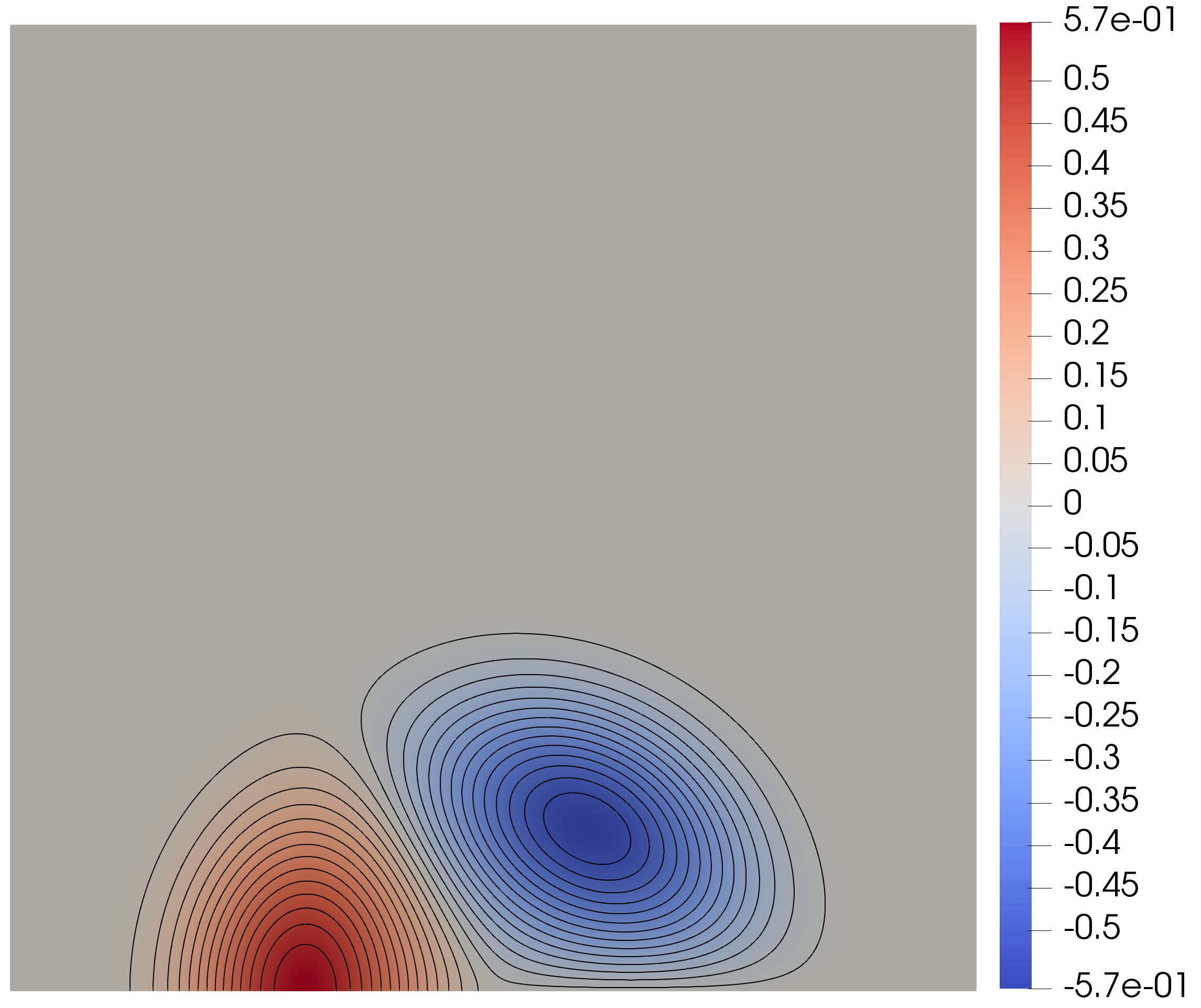
(a) Contour plot of adaptive approximation.

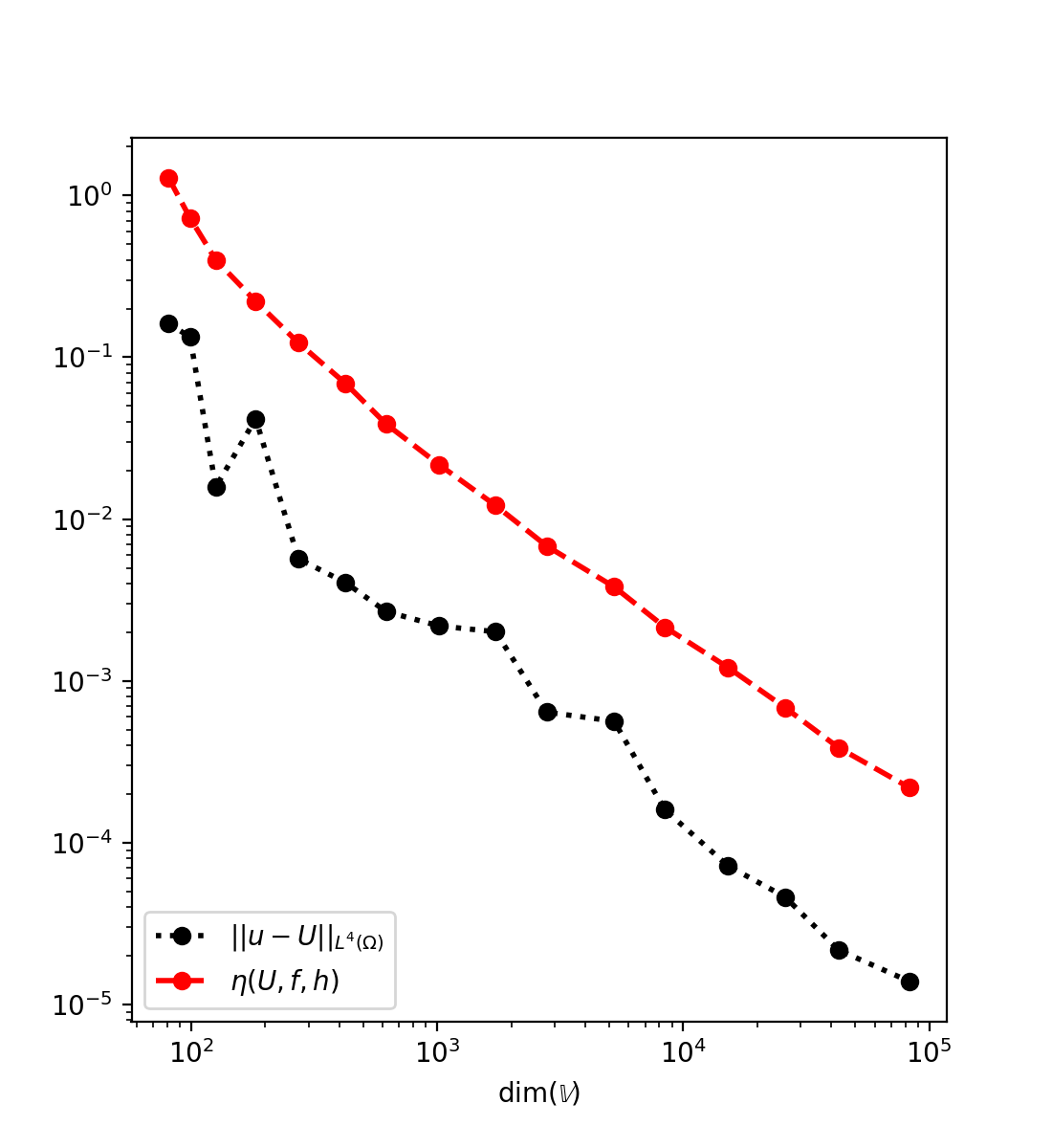
(b) Behaviour of error estimate.

(c) $\mathcal{T}^{4}$

(d) $\mathcal{T}^{8}$

(e) $\mathcal{T}^{12}$

(f) $\mathcal{T}^{15}$

Figure 3: Example 1 §5.1, contour plot and various iterations of the adaptive mesh $\mathcal{T}^{i}$ of an approximation to a function $u\in\operatorname{H}^{2}(\Omega)$. Figure 3(b) shows a double-logarithmic plot comparing the error in $\operatorname{L}^{4}(\Omega)$ (black line) with the error estimate (red line).

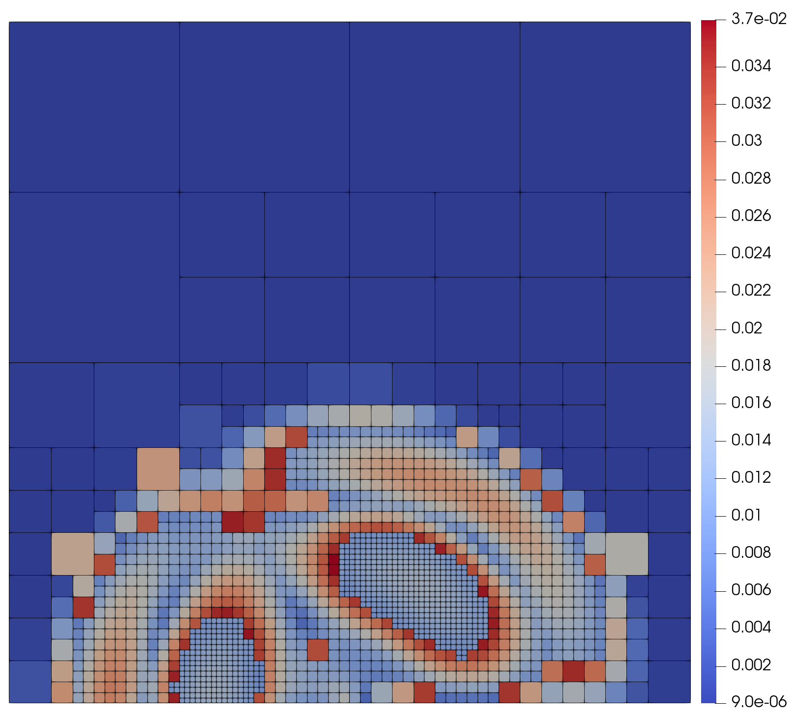
(a) Example 1. Spatial distribution of contributions to $\operatorname{L}^{32}(\Omega)$ error estimate .

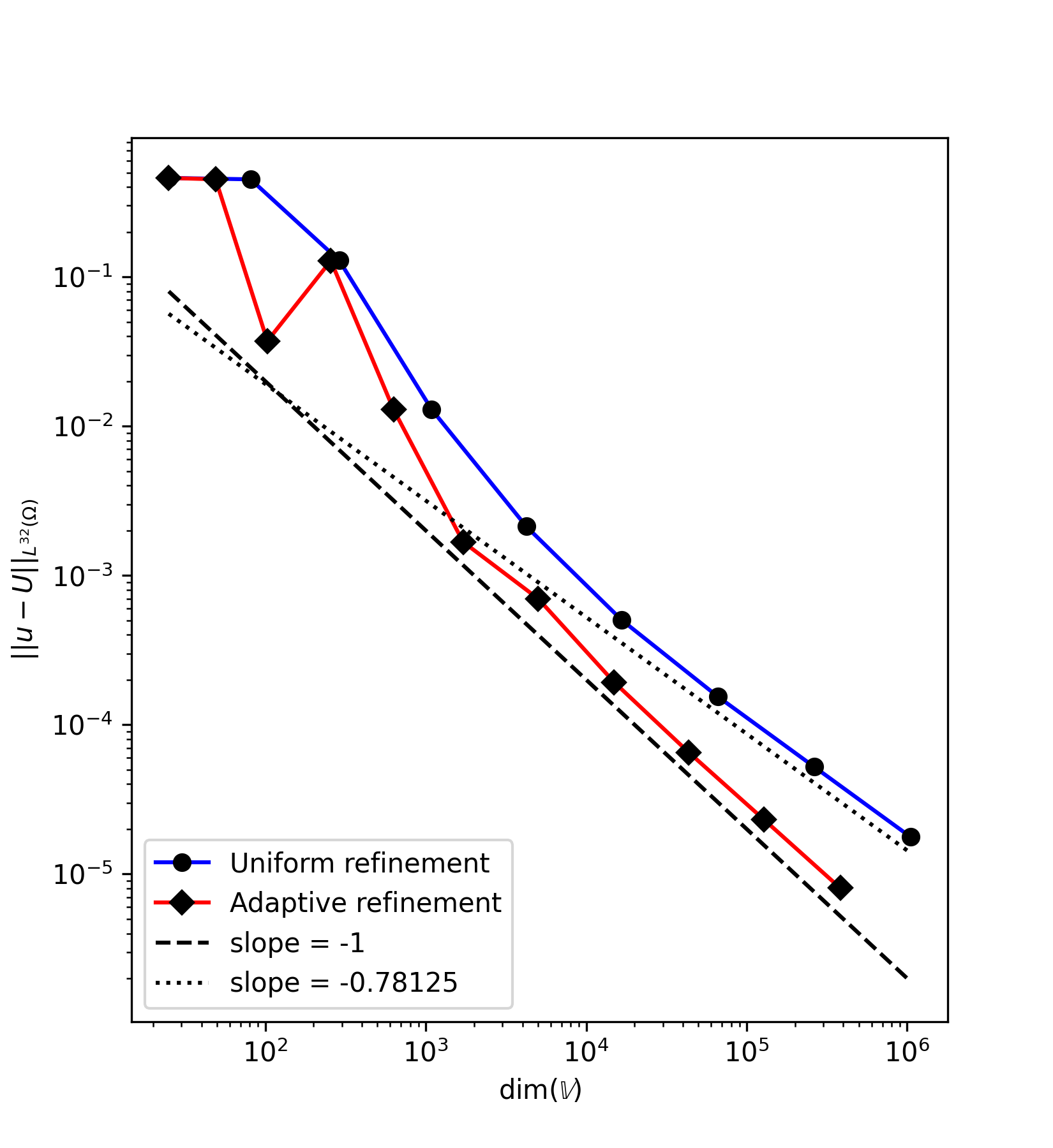
(b) Example 1. Comparison of adaptive and uniform refinement.

Figure 4: Comparison of $\operatorname{L}^{32}(\Omega)$ error computed against exact solution for uniform and adaptive meshes for example 1. Uniform mesh refinement delivers suboptimal convergence of order $h^{\tfrac{25}{16}-\varepsilon}$ as predicted by the a priori results of [16]. Optimal rates are recovered using adaptive mesh refinement.

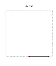
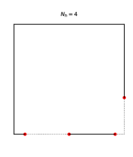
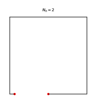
Figure 5: Example 1 §5.1, visualisation of the discrete contact set $\mathcal{A}_{U}$. Meshes $\mathcal{T}^{6}$, $\mathcal{T}^{11}$, $\mathcal{T}^{15}$. Solid line is contact (i.e. $U=0$), dashed line indicates non-contact. Critical points are shown with red dots. A boundary degree of freedom is in $\mathcal{A}_{U}$ if it is zero. For this example the discrete contact set varies on coarse meshes, and once sufficient resolution is attained we have two critical points where the boundary condition changes (note that this matches the known exact solution).

5.2 Example 2: Re-entrant Corner

To test the estimate in the presence of a geometric singularity, we introduce a re-entrant corner to the domain. In this example, data $f$ is chosen to ensure that both boundary constraints are active. The problem data is selected to try and force the solution to be close to

$$w:=\sin(2\pi(r-b)^{2})-0.5,$$ (5.5)

where $r=(x^{2}+y^{2})^{\frac{1}{2}}$ and $b$ can be varied to force different behaviours of the solution. For this example we make the choice $b=0.91$ and set $f=\Delta w+w$.

A numerical solution to this problem is shown in Figure 6(a). Under uniform mesh refinement, the error estimate converges to zero at a suboptimal rate. Optimality is restored using an adaptive routine utilising Dörfler marking with refinement fraction of 0.8 and no coarsening. A sample of the meshes produced is given in Figures 6(b)-6(e). The behaviour of the error estimate under uniform and adaptive refinement is shown in Figure 8. The slopes of the error-reduction curves reveal suboptimal convergence in the uniform case which is somewhat recovered by adaptive mesh refinement, but to different degrees. This time we see most refinement around gradients and features in the solution. Interestingly, there is little refinement around the re-entrant corner where the solution is expected to lose regularity. Instead, the error estimate prioritises resolution of the solution near where the boundary constraints are active. This simulation was performed with the Dörfler marking criterion with refine fraction 0.8 and no coarsening. The algorithm was initialised on a coarse uniform mesh with $h=1/16$.

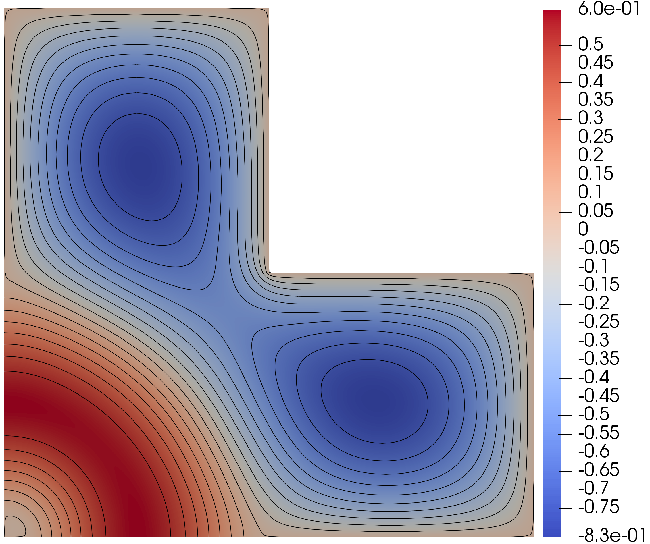
(a) Contours of $U$.

(b) $\mathcal{T}^{3}$

(c) $\mathcal{T}^{8}$

(d) $\mathcal{T}^{12}$

(e) $\mathcal{T}^{15}$

Figure 6: Example 2 §5.2, contour plot and various iterations of the adaptive mesh $\mathcal{T}^{i}$ of an approximation to a function $u\in\operatorname{W}^{2,(4-\varepsilon)/3}(\Omega)\backslash\operatorname{H}^{2}(\Omega)$. The gradient appears to be discontinuous at the corner. In this case the mesh refines around the reentrant corner as well as along qualitative features of the solution and where the boundary conditions change type.

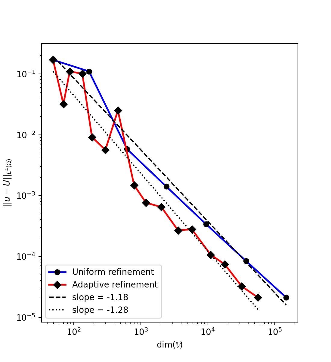
(a) Example 1. Expected slope from theory is -1.

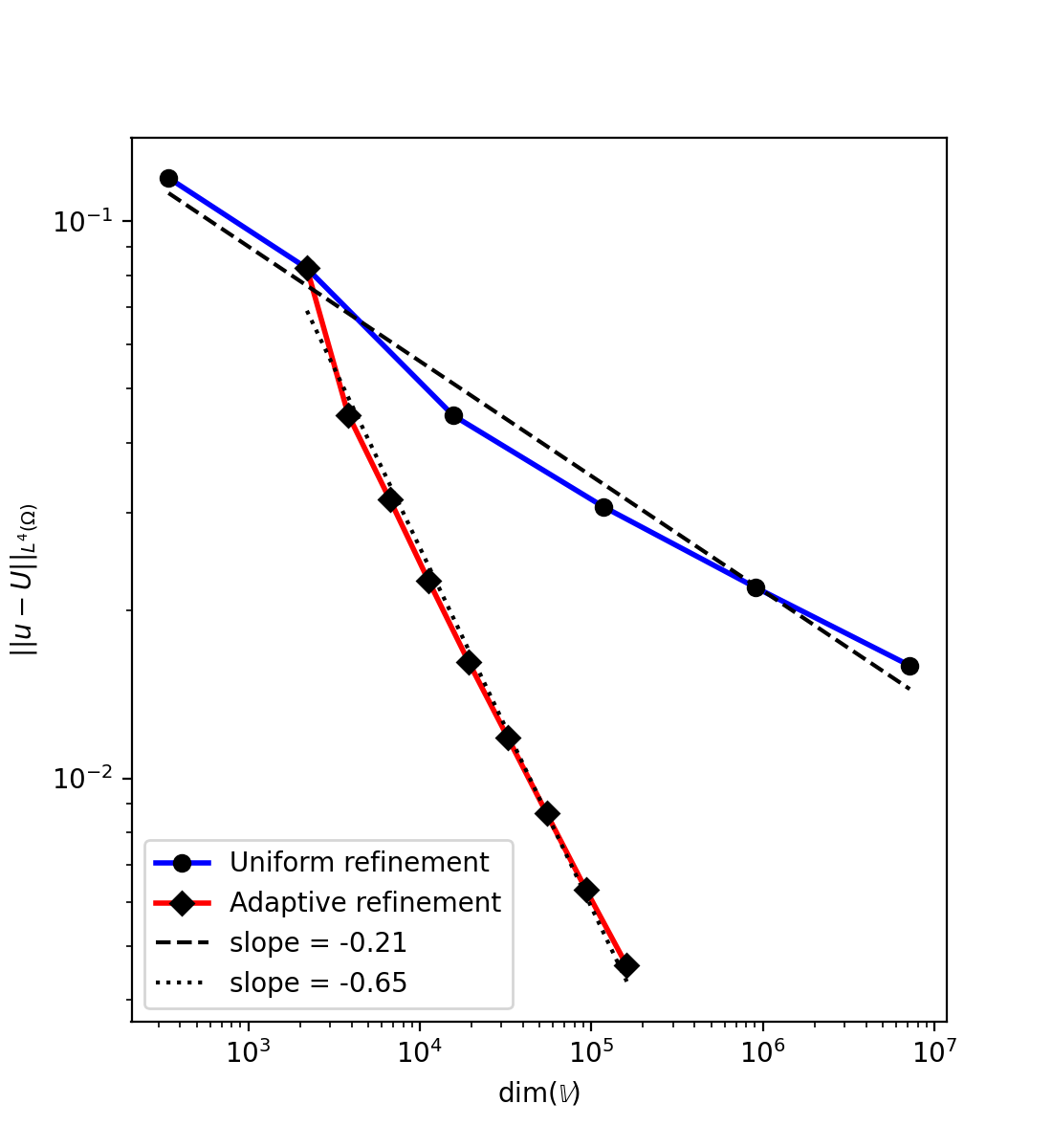
(b) Example 3. Expected slope from theory is $-\tfrac{2}{3}$.

Figure 7: Comparison of $\operatorname{L}^{4}(\Omega)$ error computed against exact solutions for uniform and adaptive meshes for those examples for which an exact solution is available. The orders of convergence of the error estimate in each case (that is, the slope of the error values) is approximated from the log-scaled data by performing standard least squares linear regression.

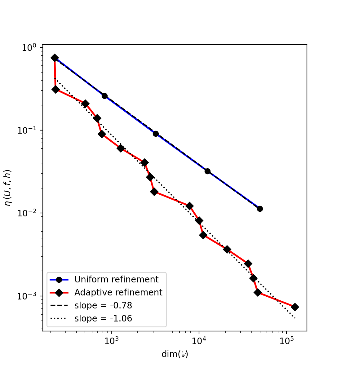
(a) Example 2. Expected slope from theory is $-1$.

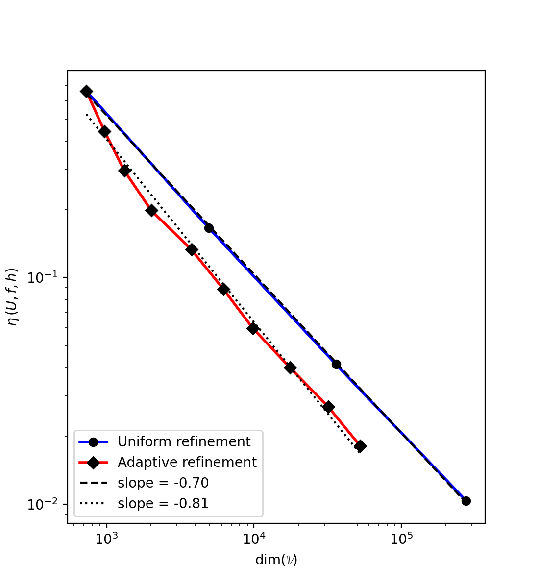
(b) Example 3. Expected slope from theory is $-\tfrac{2}{3}$.

Figure 8: Double logarithmic plot of error estimate against number of degrees of freedom under uniform and adaptive mesh refinement for examples 2 and 3, that is, the examples that do not meet the necessary assumptions for the theory above to hold. The orders of convergence of the error estimate in each case is approximated from the log-scaled data by performing standard least squares linear regression.

5.3 Example 3, $d=3$.

Working in three dimensions and in spherical polar coordinates, centred at $(0.5,0,0.5)$, we now consider a test analogous to example 1. Let $(r,\theta,\phi)$ denote spherical polar coordinates centred at $(0.5,0,0)$. We note that the function

$$u=-10\psi(r)r^{3/2}\sin\left(\frac{3}{2}\varphi\right)\sin\left(\frac{3}{4}\theta\right)$$ (5.6)

satisfies appropriate constraints on the boundary and so solves (1.1), (1.2) for appropriately defined $f$. Contours of (5.6) are shown in Figure 9. Again we use Dörfler marking with refine fraction of $0.8$ and no coarsening.

Adaptive meshes from several stages of the adaptive algorithm are displayed in 10 (note that these are slices of a three-dimensional mesh). We observe that mesh resolution is greater close to the boundary where the Signorini constraints are active (in this case the plane defined by $y=0$) and provides good resolution of the contact set. Refinement is also present around key features of the solution, as observed for example 1, Figures 3(a) and 3(c)-3(f)

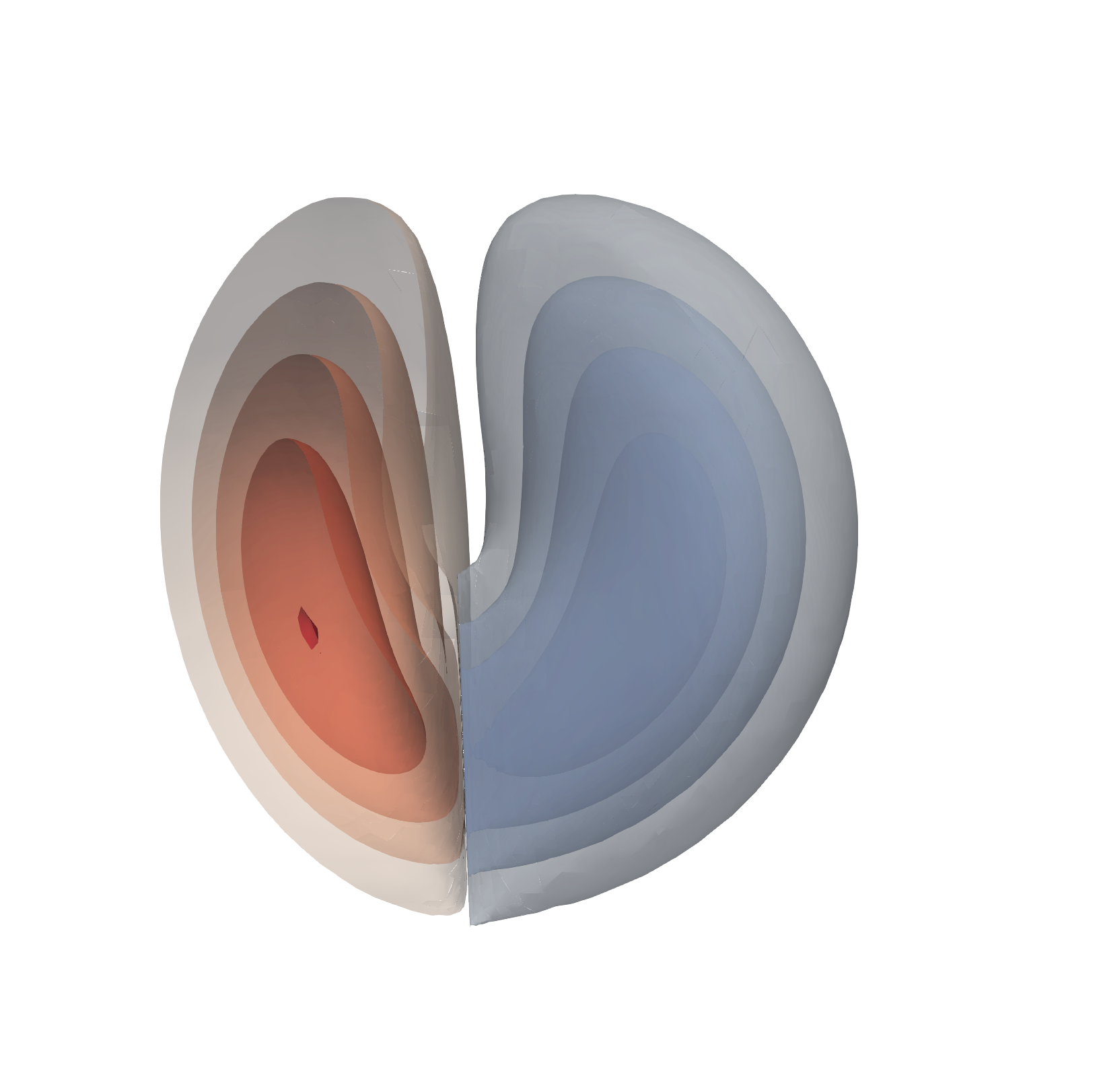
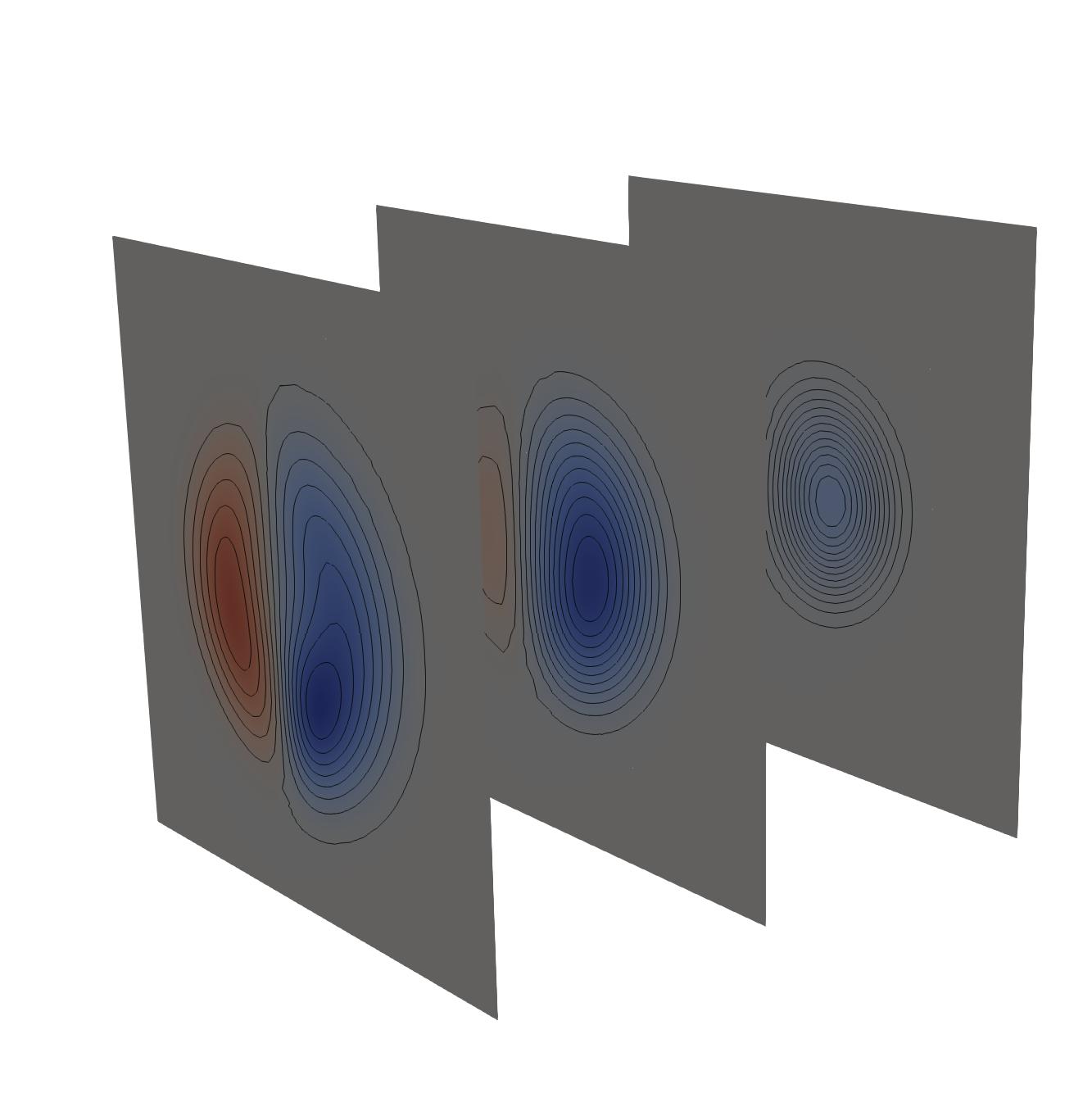
Figure 9: Left: contours of the numerical solution to example 3 §5.3, Right: slices of the numerical solution parallel to planes $y=c$ for $c=0.1,0.2$ and 0.3. Note that for visualisation purposes the right hand plot is not to scale; the planes have been translated along the $y$-axis.

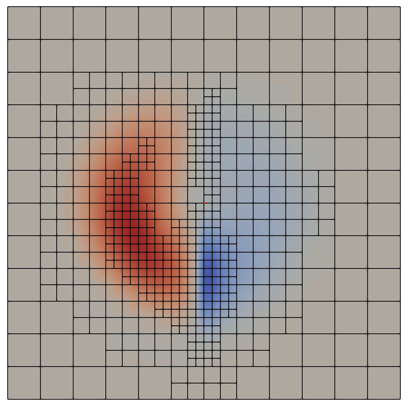
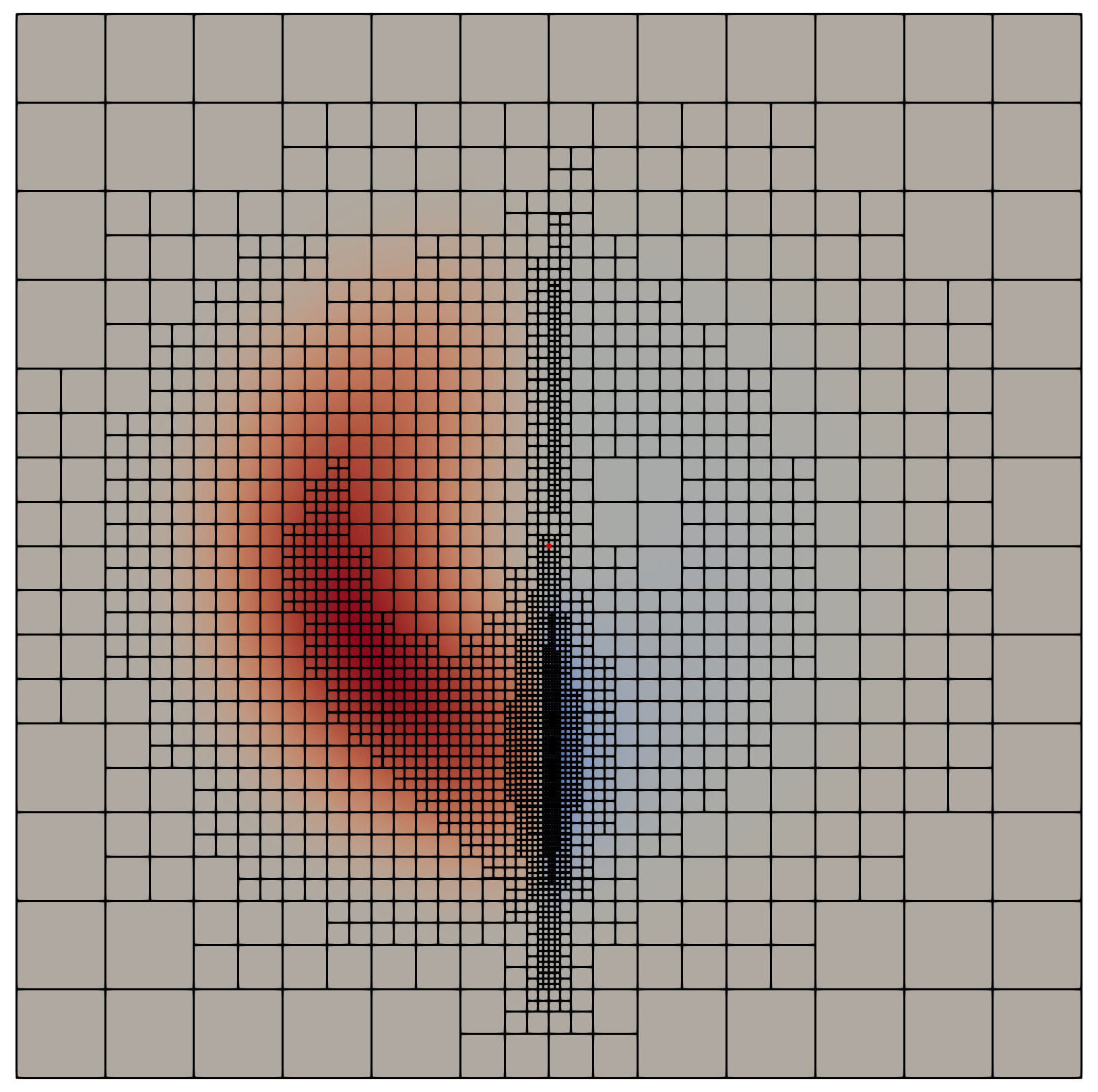
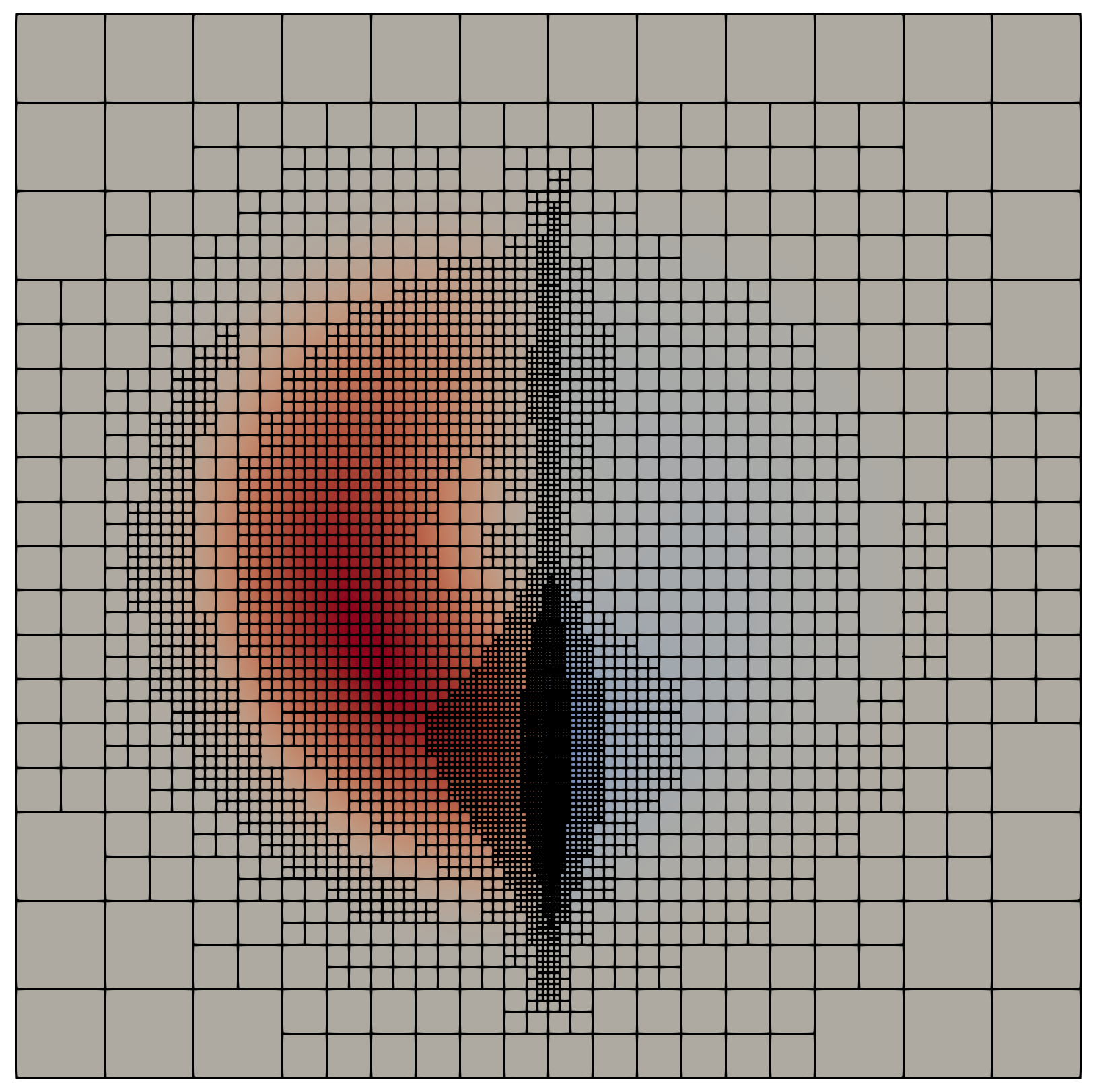
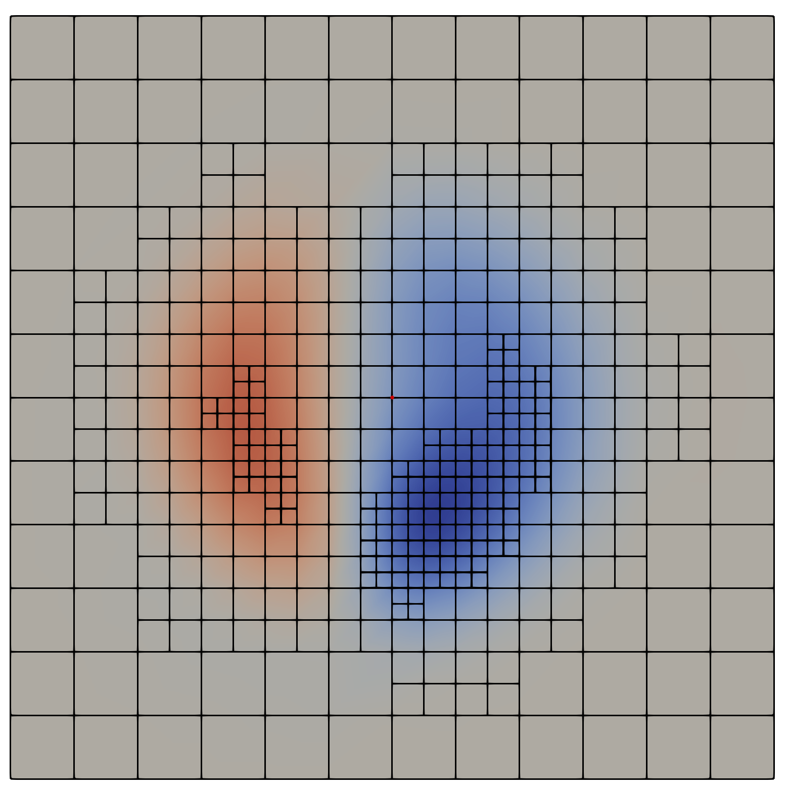
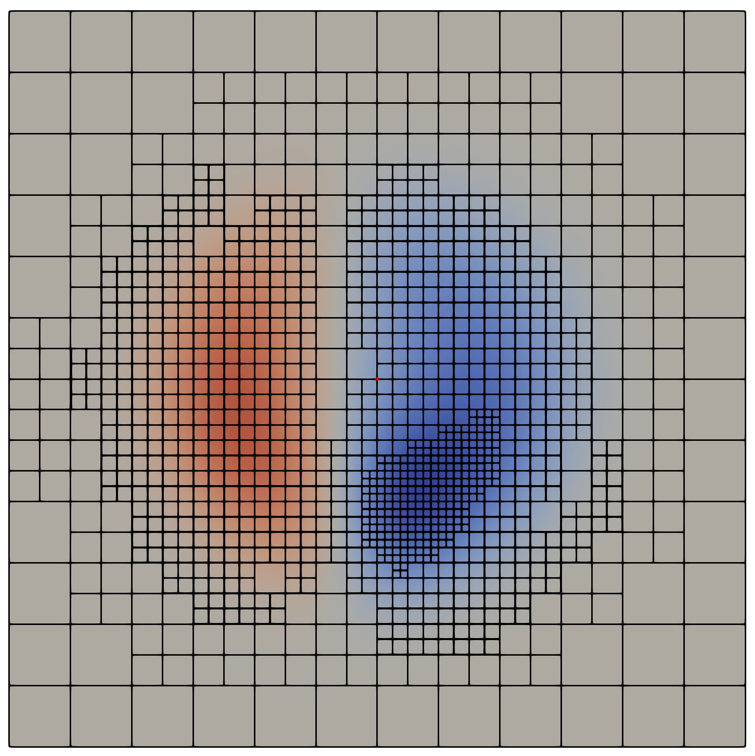
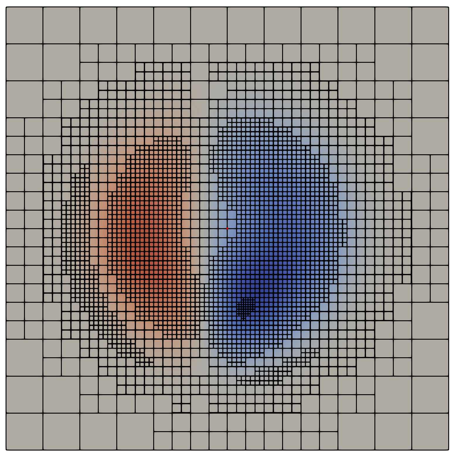
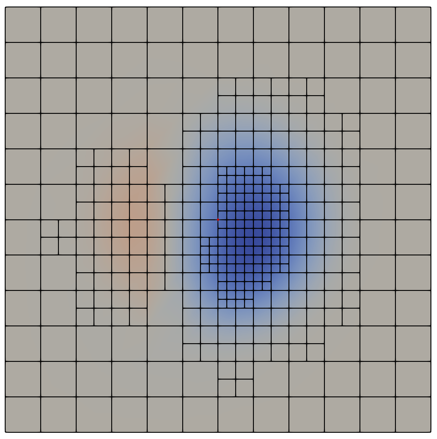
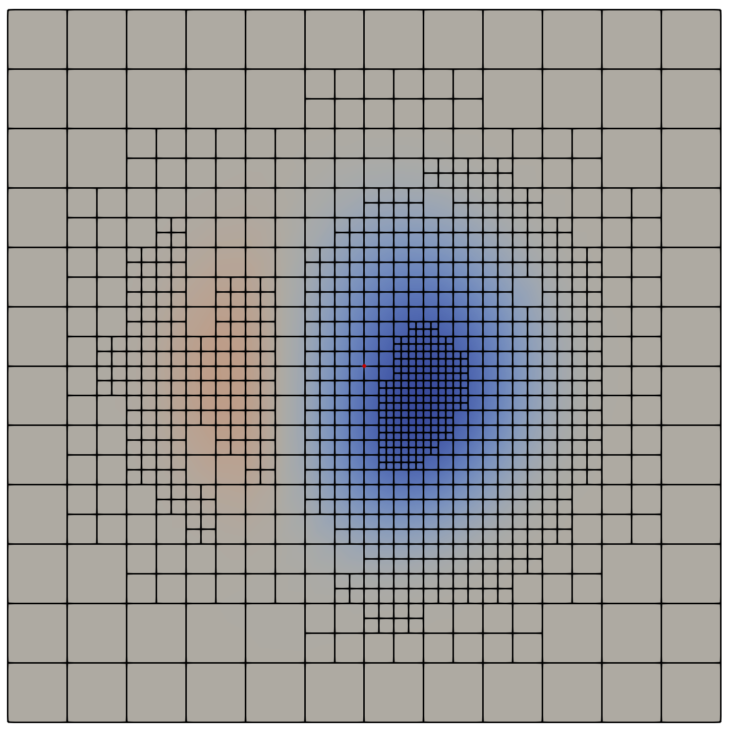
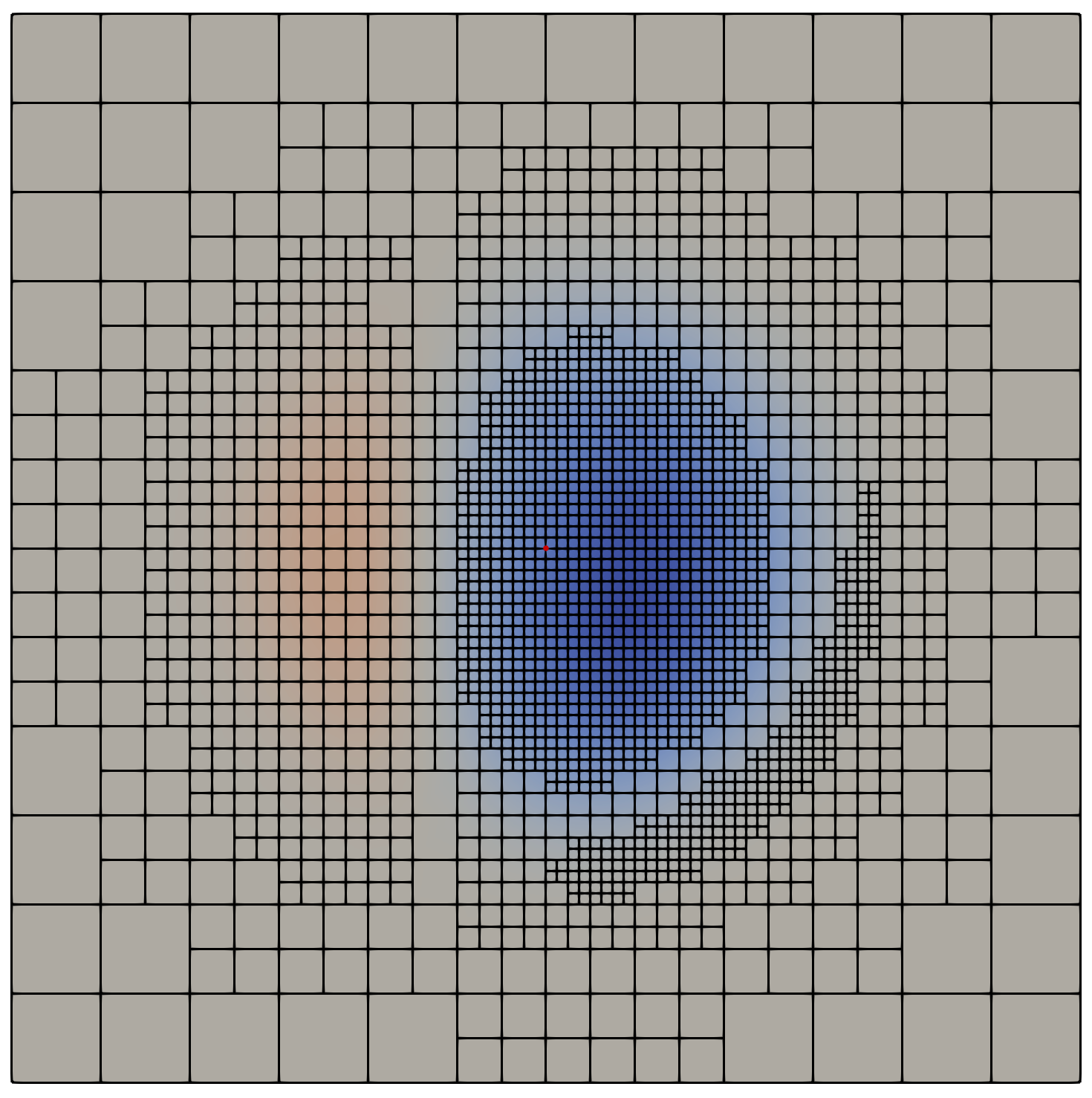
Figure 10: Adaptively generated meshes for example 3. The slices shown are the intersections of the mesh with the planes $y=0.01$ (top row), $y=0.1$, (middle row) and $y=0.2$ (bottom row) and show the mesh after refinement cycles 2 (left hand column), 5 (middle column) and 8 (right hand column). The mesh is heavily refined along the $z$ axis due to both active boundary constraints and gradient singularities in the solution.

6 Conclusions & discussion

In this article, rigorous error estimates were derived for the scalar Signorini problem in non-energy norms, specifically $\operatorname{L}^{p}(\Omega)$ with $p\in(4,\infty)$, using a duality argument. The a posteriori error estimates were benchmarked against known exact solutions and shown to have the same asymptotic rates as the a priori analysis, and to be sharp to a satisfactory degree (overestimation factor of approximately 20). Adaptive mesh refinement was shown to decrease error for a given number of degrees of freedom compared to uniform meshes, particularly for a challenging three-dimensional problem. Furthermore, since asymptotic convergence is suboptimal in $\operatorname{L}^{p}(\Omega)$ for large $p$ we demonstrated that adaptive schemes are able to regain optimal rates in terms of the number of degrees of freedom.

The error estimate was tested on more challenging test cases, both in situations where the assumptions of the main theorem were satisfied, and in a case where they were not (three spatial dimensions, re-entrant corners). In the three-dimensional case where the theory does not hold (see Section 5.3 and Figure 8(b)), we remark that the error estimate is too optimistic in the sense that the error estimate decreases at the expected rate under uniform refinement, whereas the error does not (see Figure 7(b)). This means that although adaptivity did produce superior error reduction in this case, it can only be used as an indicator, not an estimator.

This work presents many avenues for further investigation which include the analysis in higher spatial dimensions, as already indicated. Further work is underway on nontrivial obstacles as well as the generalisation to higher polynomial degrees. While we do not believe the bilateral interpolation result can be true globally, which is critical to the analysis, we note the recent work [5] where the authors give an alternative nodal interpretation that may shed some light on the quest for higher order methods.

References

- [1] Mark Ainsworth and J Tinsley Oden “A posteriori error estimation in finite element analysis” John Wiley & Sons, 2011
- [2] Thomas Apel and Serge Nicaise “Regularity of the solution of the scalar Signorini problem in polygonal domains” In Results in Mathematics 75.2 Springer, 2020, pp. 1–15
- [3] Daniel Arndt et al. “The deal.II library, version 9.1” In Journal of Numerical Mathematics 27.4 De Gruyter, 2019, pp. 203–213
- [4] Ben Ashby, Cassiano Bortolozo, Alex Lukyanov and Tristan Pryer “Adaptive modelling of variably saturated seepage problems” In The Quarterly Journal of Mechanics and Applied Mathematics 74.1 Oxford University Press, 2021, pp. 55–81
- [5] Gabriel R Barrenechea, Emmanuil Georgoulis, Tristan Pryer and Andreas Veeser “A nodally bound-preserving finite element method” In IMA Journal of Numerical Analysis Oxford University Press, 2023
- [6] Faker Ben Belgacem, Patrick Hild and Patrick Laborde “Extension of the mortar finite element method to a variational inequality modeling unilateral contact” In Mathematical Models and Methods in Applied Sciences 9.02 World Scientific, 1999, pp. 287–303
- [7] Zakaria Belhachmi and F Belgacem “Quadratic finite element approximation of the Signorini problem” In Mathematics of computation 72.241, 2003, pp. 83–104
- [8] F Ben Belgacem “Numerical simulation of some variational inequalities arisen from unilateral contact problems by the finite element methods” In SIAM Journal on Numerical Analysis 37.4 SIAM, 2000, pp. 1198–1216
- [9] H. Blum and F.T. Suttmeier “An adaptive finite element discretisation for a simplified Signorini problem” In Calcolo 37.2, 2000, pp. 65–77
- [10] Dietrich Braess “A posteriori error estimators for obstacle problems–another look” In Numerische Mathematik 101.3 Springer, 2005, pp. 415–421
- [11] S.. Brenner and L.. Scott “The Mathematical Theory of Finite Element Methods” Springer Science & Business Media, 2008
- [12] F Brezzi and G Sacchi “A finite element approximation of a variational inequality related to hydraulics” In Calcolo 13.3 Springer, 1976, pp. 257–273
- [13] Franco Brezzi, William W Hager and PA Raviart “Error estimates for the finite element solution of variational inequalities: Part I. Primal theory” In Numerische Mathematik 28.4 Springer, 1977, pp. 431–443
- [14] Franco Brezzi, William W Hager and PA Raviart “Error estimates for the finite element solution of variational inequalities: Part II. Mixed methods” In Numerische Mathematik 31.1 Springer, 1978, pp. 1–16
- [15] Zhiming Chen and Ricardo H. Nochetto “Residual type a posteriori error estimates for elliptic obstacle problems” In Numerische Mathematik 84.4, 2000, pp. 527–548
- [16] Constantin Christof and Christof Haubner “Finite element error estimates in non-energy norms for the two-dimensional scalar Signorini problem” In Numerische Mathematik 145.3 Springer, 2020, pp. 513–551
- [17] Ph Clément “Approximation by finite element functions using local regularization” In Revue française d’automatique, informatique, recherche opérationnelle. Analyse numérique 9.R2 EDP Sciences, 1975, pp. 77–84
- [18] Ronald A DeVore “Nonlinear approximation” In Acta numerica 7 Cambridge University Press, 1998, pp. 51–150
- [19] W. Dörfler “A Convergent Adaptive Algorithm for Poisson’s Equation” In SIAM J. Numer. Anal. 33.3, 1996, pp. 1106–1124
- [20] Guillaume Drouet and Patrick Hild “Optimal convergence for discrete variational inequalities modelling Signorini contact in 2D and 3D without additional assumptions on the unknown contact set” In SIAM Journal on Numerical Analysis 53.3 SIAM, 2015, pp. 1488–1507
- [21] A Ern and JL Guermond “Finite Elements I: Approximation and interpolation” Springer, 2021
- [22] R.. Falk “Error estimates for the approximation of a class of variational inequalities” In Mathematics of Computation 28.128, 1974, pp. 963–971
- [23] Pierre Grisvard “Elliptic problems in nonsmooth domains” SIAM, 1985
- [24] Jaroslav Haslinger, Ivan Hlaváček and Jindřich Nečas “Numerical methods for unilateral problems in solid mechanics” In Handbook of numerical analysis 4 Elsevier, 1996, pp. 313–485
- [25] Patrick Hild and Serge Nicaise “A posteriori error estimations of residual type for Signorini’s problem” In Numerische Mathematik 101.3 Springer, 2005, pp. 523–549
- [26] Patrick Hild and Yves Renard “An improved a priori error analysis for finite element approximations of Signorini’s problem” In SIAM Journal on Numerical Analysis 50.5 SIAM, 2012, pp. 2400–2419
- [27] Ronald HW Hoppe and Ralf Kornhuber “Adaptive multilevel methods for obstacle problems” In SIAM journal on numerical analysis 31.2 SIAM, 1994, pp. 301–323
- [28] Stefan Hüeber and Barbara I Wohlmuth “An optimal a priori error estimate for nonlinear multibody contact problems” In SIAM Journal on Numerical Analysis 43.1 SIAM, 2005, pp. 156–173
- [29] David Kinderlehrer and Guido Stampacchia “An introduction to variational inequalities and their applications” SIAM, 2000
- [30] Rolf Krause, Andreas Veeser and Mirjam Walloth “An efficient and reliable residual-type a posteriori error estimator for the Signorini problem” In Numerische Mathematik 130.1 Springer, 2015, pp. 151–197
- [31] J.-L. Lions and G. Stampacchia “Variational inequalities” In Communications on pure and applied mathematics 20.3 Wiley Online Library, 1967, pp. 493–519
- [32] U Mosco “Error estimates for some variational inequalities” In Mathematical Aspects of Finite Element Methods Springer, 1977, pp. 224–236
- [33] Umberto Mosco and Gilbert Strang “One-sided approximation and variational inequalities” In Bulletin of the American Mathematical Society 80.2 American Mathematical Society, 1974, pp. 308–312
- [34] Joachim Nitsche “-convergence of finite element approximations” In Mathematical aspects of finite element methods Springer, 1977, pp. 261–274
- [35] Ricardo H. Nochetto, Kunibert G. Siebert and Andreas Veeser “Pointwise a posteriori error control for elliptic obstacle problems” In Numerische Mathematik 95.1, 2003, pp. 163–195
- [36] Francesco Scarpini and Maria Agostina Vivaldi “Error estimates for the approximation of some unilateral problems” In RAIRO. Analyse numérique 11.2 EDP Sciences, 1977, pp. 197–208
- [37] L Ridgway Scott and Shangyou Zhang “Finite element interpolation of nonsmooth functions satisfying boundary conditions” In Mathematics of computation 54.190, 1990, pp. 483–493
- [38] Olaf Steinbach, Barbara Wohlmuth and Linus Wunderlich “Trace and flux a priori error estimates in finite-element approximations of Signorni-type problems” In IMA Journal of Numerical Analysis 36.3, 2015, pp. 1072–1095
- [39] Gilbert Strang “One-sided approximation and plate bending” In Computing Methods in Applied Sciences and Engineering Part 1 Springer, 1974, pp. 140–155
- [40] Gilbert Strang “The dimension of piecewise polynomial spaces, and one-sided approximation” In Conference on the Numerical Solution of Differential Equations, 1974, pp. 144–152 Springer
- [41] F.-T. Suttmeier “Numerical solution of variational inequalities by adaptive finite elements” Springer, 2008
- [42] Andreas Veeser “Approximating gradients with continuous piecewise polynomial functions” In Foundations of Computational Mathematics 16.3 Springer, 2016, pp. 723–750
- [43] Andreas Veeser “Positivity preserving gradient approximation with linear finite elements” In Computational Methods in Applied Mathematics 19.2 De Gruyter, 2019, pp. 295–310
- [44] Mirjam Walloth “A reliable, efficient and localized error estimator for a discontinuous Galerkin method for the Signorini problem” In Applied Numerical Mathematics 135 Elsevier, 2019, pp. 276–296
- [45] Alexander Weiss and Barbara I Wohlmuth “A posteriori error estimator for obstacle problems” In SIAM Journal on Scientific Computing 32.5 SIAM, 2010, pp. 2627–2658
- [46] Chensong Zhang “Adaptive finite element methods for variational inequalities: Theory and applications in finance”, 2007