FireANTs: Adaptive Riemannian Optimization
for Multi-Scale Diffeomorphic Registration

Abstract

Diffeomorphic Image Registration is a critical part of the analysis in various imaging modalities and downstream tasks like image translation, segmentation, and atlas building. Registration algorithms based on optimization have stood the test of time in terms of accuracy, reliability, and robustness across a wide spectrum of modalities and acquisition settings. However, these algorithms converge slowly, are prohibitively expensive to run, and their usage requires a steep learning curve, limiting their scalability to larger clinical and scientific studies. In this paper, we develop multi-scale Adaptive Riemannian Optimization algorithms for diffeomorphic image registration. We demonstrate compelling improvements on image registration across a spectrum of modalities and anatomies by measuring structural and landmark overlap of the registered image volumes. Our proposed framework leads to a consistent improvement in performance, and from 300$\times$ up to 2000$\times$ speedup over existing algorithms. Our modular library design makes it easy to use and allows customization via user-defined cost functions.

Keywords: image registration, image matching, image alignment, diffeomorphisms, multi-scale optimization, scalability, MRI, computed tomography, microscopy

1 Main

Deformable Image Registration is one of the most ubiquitous tasks in image analysis. It refers to the non-linear and local (hence deformable) alignment of two or more images into a common coordinate system. Depending on the problem and modality, the images can be sourced from different subjects or events, modalities, and timepoints. Image registration is routinely used in neuroimaging  ^{1, 2, 3, 4, 5}, cardiac imaging  ^{6, 7, 8}, lung imaging  ^{9, 10, 11}, microscopy and histology  ^{12, 13, 14, 15, 16} to name a few biomedical applications. In neuroimaging, inter-subject registration is used to align structural regions for automatic segmentation, or to construct an anatomical template (atlas) for anomaly detection or deviations from a healthy population. In lung imaging, registration is used to understand the dynamics of the lung deformation during inspiration-expiration, or to track lesions over temporally spaced breathhold scans. Image registration is used in microscopy ^{12, 13, 16} to compensate for the large deformations that occur between staining rounds, and stitching misaligned 2D histology slides to generate a 3D volume. We note that registration is often used beyond biomedical applications; in planetary image alignment  ¹⁷, satellite imagery and remote sensing  ^{18, 19, 20}, robotics  ^{21, 22, 23}, and astronomy  ^{24, 25, 26} and traditional computer vision applications like optical flow ^{27, 28, 29, 30}. In this paper, we focus on image registration for biomedical applications, including microscopy, Magnetic Resonance Imaging (MRI), and Computed Tomography (CT) imaging, but our method is more generally applicable to other imaging as well.

Image registration methods are typically divided into two categories – optimization-based and learning-based. Optimization-based methods focus on mathematically formulating registration as a variational optimization problem. This involves selecting a dissimilarity function between the reference and warped image, the family of deformation fields over which to optimize, and the optimization algorithm to use. In the literature, the reference and warped images are typically called fixed and moving images respectively. Diffeomorphisms are of special interest as a family of deformations, which are invertible transformations such that both the transform and its inverse are differentiable. Some of the earliest approaches considered models for small deformations  ^{31, 32, 33, 34, 35}. Other approaches perform gradient based optimization on the variational objective function  ^{36, 37, 38, 39}, modelling diffeomorphisms as solutions of a differential equation with a time-dependent velocity field ⁴⁰, followed up with geodesic formulations ^{41, 42, 43}, and direct integration of the velocity fields using gradient descent ^{44, 45}. These methods focus on the representation choice and optimization technique. An orthogonal problem in image registration is the lack of discriminative features in medical images which are noisy and contain artifacts, making intensity based registration susceptible to local minima and slow convergence. To overcome these problems, learning based methods train a deep neural network that inputs the intensity images and predicts the deformation directly ^{46, 47, 48, 49, 50, 9, 51, 52}. These deep networks are trained with the loss functions and deformation representations proposed in optimization based methods, but instead of iterating to find the optimal deformation, it is predicted directly. Such methods can be thought of as converting the homogenous and noisy intensity images into a feature image that is used to predict the deformation in a single step. Optimization methods study the family of deformations, their representations (elastostatics, viscous fluid, underlying Lie algebra, etc.) and how to optimize them, and learning focuses on automatic featurization of the intensity image that are conducive to registration.

Despite the extensive literature, Diffeomorphic Image Registration remains an active research area due to its high-dimensional solution space, ill-conditioned optimization, and non-Euclidean manifold of the transformation space. The significance of our work stems from the observation that these problems remain unaddressed by state-of-the-art optimization based registration methods, which typically use Gradient Descent ^{40, 53, 45} to optimize diffeomorphisms. In particular, first-order adaptive optimization methods are shown to speed up convergence in ill-conditioned optimization problems ^{54, 55, 56} without computing expensive second-order terms. Although first-order adaptive optimization methods have shown faster convergence to better local minima in fixed-dimensional Euclidean parameter spaces ^{55, 54, 56} (i.e. deep learning) and fixed low-dimensional non-Euclidean manifolds ^{57, 58, 59}, these optimizers do not exist for diffeomorphic registration. This is because the size of the transform depends on the size of the image and changes over multi-scale optimization. We implement a novel multi-scale Adaptive Riemannanian optimization for Diffeomorphic Registration to mitigate the high-dimensional, ill-conditioned, non-Euclidean optimization problem. We introduce key technical contributions (Section 4) to avoid computing terms like the Riemannian Metric Tensor, and Parallel Transport of the optimization state, which are computationally expensive and not feasible for high-dimensional diffeomorphisms. To our knowledge, we are the first to implement a multi-scale Riemannian Adaptive Optimization algorithm for diffeomorphic registration. This leads to a state-of-the-art adaptive optimization algorithm for diffeomorphic registration(Figs. 2 and 3).

Our work also addresses the lack of scalability of existing registration algorithms. Existing optimization toolkits ^{60, 53, 61, 62} have prohibitively slow runtimes, which limits their applicability to hyperparameter studies for novel modalities or high-resolution images. Deep learning methods provide very fast runtimes but have steep compute and memory requirements, making them infeasible for high-resolution registration. Most deep learning methods perform registration on low-resolution image volumes ⁶³ of size 160$\times$192$\times$224 voxels, which is much smaller than CT scans in EMPIRE10 ¹⁰ (up to 420$\times$ 312 $\times$ 537 voxels) and RnR-ExM ⁶⁴ (2048$\times$2048$\times$81 voxels) challenges. Most notably, for modalities like microscopy, existing methods ^{52, 62} either downsample the image volume by up to $64\times$ or register image chunks independently. This aggressive downsampling or chunking leads to substantial loss of rich image features necessary for accurate registration. Our method can register these volumes at native resolution (Fig. 4), introducing a new benchmark for accurate and scalable image registration algorithms. This scalability also makes large-scale hyperparameter studies more computationally feasible (Figs. 6 and 5).

Our key contributions are as follows: first, we propose a novel multi-scale Adaptive Riemannan Optimization framework for diffeomorphisms. Our framework leverages mathematical correspondences to avoid expensive operations like the Riemannanian Metric Tensor and Parallel Transport which are needed for implementing first-order adaptive algorithms. This leads to a state-of-the art optimization algorithm that is accurate, fast and robust across various registration settings. Second, we accompany the method with a Python library that is easy to use and extend, and is packaged with optimizers for other transforms like rigid and affine transforms. Similar to existing toolkits ⁶⁰, our method can compose transformations, avoiding resampling artifacts across transformations. This is designed to push the frontier of scalability in image registration algorithms. Our method scales in time, leading to up to a 3200 $\times$ speedup over existing state-of-the-art toolkits (Fig. 5) and scales in resolution, performing diffeomorphic registration on microscopy images at native resolution (Fig. 4). Our implementation is agnostic to modality, resolutions, and is not sensitive to hyperparameters, making it a versatile benchmark for diverse applications.

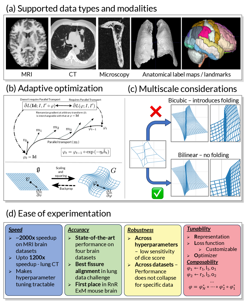
Figure 1: Overview of FireANTs and its features: (a) shows the modalities our method is tested on. We demonstrate results on in-vivo T1-weighted brain MRI, lung CT, and expansion microscopy volumes. FireANTs can optimize intensity images as well as binary masks (lung masks in CT) or entire anatomical label maps (brain MRI). (b) shows the technical contributions of FireANTs. We extend Adaptive Optimization to multi-scale Diffeomorphisms by first writing the Riemannian gradient update, and then avoiding parallel transport of the optimization state by leverging the interchangability of the Riemannian gradient at arbitrary transform $\varphi_{t}$ with the Riemannian gradient at $\varphi=\textbf{Id}$. For the Lie-algebra representation, the Gateaux derivative $\frac{\partial L}{\partial\varphi}$ is projected to $\frac{\partial L}{\partial v}$ using analytical backprop. Since the Lie algebra is a vector space, we use standard adaptive optimizers (see Section 4 for more details). (c) takes a closer look at multi-scale interpolation for diffeomorphisms represented as a warp field. Bicubic interpolation can introduce folding of the warp field at a finer resolution due to overshooting, but bilinear interpolation does not. Therefore, we use this for interpolating the warp field and the optimizer state. (d) shows the extensive experimental setup. Our method is orders of magnitude faster, has state-of-the-art performance on 3 challenges, is robust across hyperparameters and datasets, and is modular and easy to extend.

2 Results

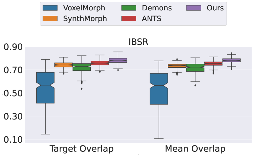
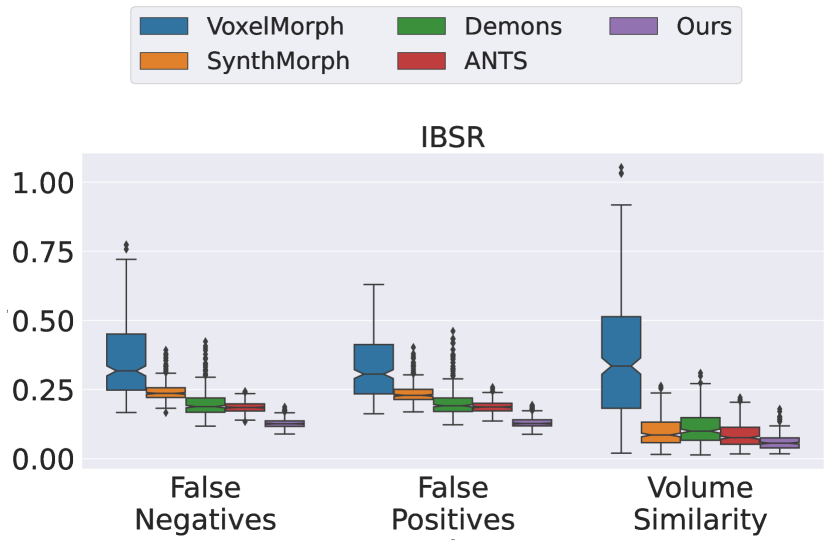
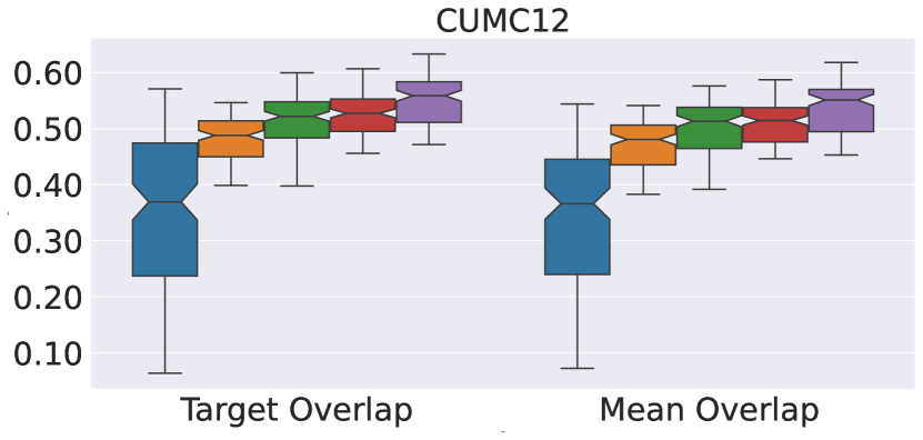
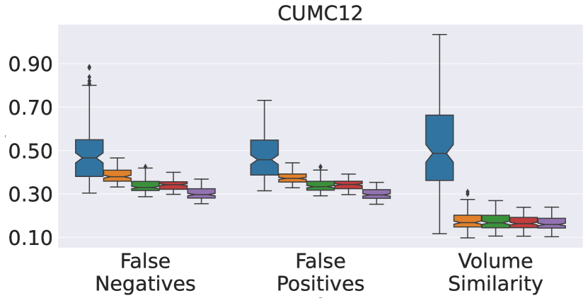
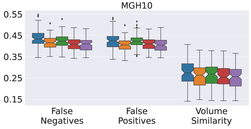
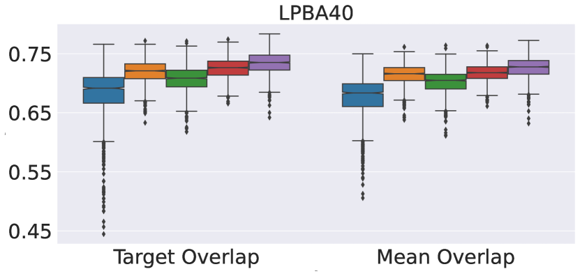
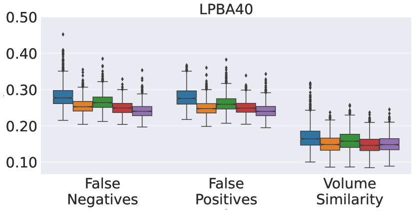
Figure 2: FireANTs demonstrates state-of-the-art performance on Klein et al.challenge ⁵ : Registration quality is validated by measuring the average volume overlap measurements of all anatomical label maps between the fixed and warped label maps (see Section 4.1 for description of all metrics used). Our method outperforms state-of-the-art registration algorithms, including ANTs which was the top performing method in the challenge, and deep learning algorithms like VoxelMorph and SynthMorph. For deep learning baselines, appropriate preprocessing (intensity normalization, alignment, and resampling to 1mm isotropic) is performed to ensure a fair comparison, whereas no such preprocessing is required for optimization methods, including FireANTs. Boxplots show that the gains in performance are consistent across all four datasets, with the median overlap scores outperforming the third quartile of all other methods for IBSR and CUMC12 datasets. Results of per region overlap metrics are in Fig. S.1. For the overlap aggregation mentioned in ⁵, results are shown in Fig. S.2.

We validate the proposed features of our method using a comprehensive evaluation setup. First, we show that our proposed Riemannanian Adaptive Optimization leads to consistently better registration performance compared to state-of-the-art optimization algorithms that utilize Gradient Descent. This is shown on two challenges ^{5, 10} which are established community standards for evaluating registration algorithms, and present various challenges such as different modalities, anatomical regions and variations, voxel resolutions, anisotropy, and acquisition settings. Next, we demonstrate FireANTs’ scalability in resolution by performing deformation registration on high-resolution microscopy images ⁶⁴ at native resolution, which are previously registered either at a significantly lower resolution or in chunks. We also show scalability in runtime by showing speedups of upto 3 orders of magnitude compared to existing SOTA algorithms. Finally, we show that FireANTs is robust to choice of registation hyperparameters, and its signifcant speedup allows for fast hyperparameter tuning, which is otherwise infeasible with existing algorithms.

2.1 Comparison on human brain MRI registration

Analysis of functional and physiological data in neuroscience require different brain images to lie in the same coordinate space to establish correspondence across different brain regions. As such, registration algorithms are at the forefront of such analysis. Klein et al. ⁵ present a comprehensive, unbiased, and thorough evaluation of different registration algorithms on four MRI brain datasets, with Advanced Normalization Tools (ANTs) ⁶⁰ being the top performing method overall. Four datasets are used in the challenge, with a total of 80 brains. The datasets have different voxel resolutions, scanners, preprocessing pipelines, and labeled anatomical regions. More details about the dataset and evaluation protocol are discussed in  Section 4.1. The challenge therefore evaluates robustness of registration algorithms across a wide variety of dataset attributes and anatomical alignment. We compare our method with two state-of-the-art optimization algorithms: ANTs and Symmetric Log Demons ⁶¹, and two deep learning algorithms: VoxelMorph ⁴⁶ and SynthMorph ⁵¹ using their provided pretrained models. In addition to the proposed metrics in ⁵, we also propose alternate versions of the same metrics, but averaged over all the brain regions (see Section 4.1). For all the four datasets, we first fit an affine transformation from the moving image to the fixed image, followed by a diffeomorphic transform. Results for the brain datasets are shown in  Fig. 2 and  Fig. S.1.

Our algorithm outperforms all baselines on all four datasets, with a monotonic improvement in all metrics evaluating the volume overlap of the fixed and warped label maps. The improvements are consistent in all datasets, with varying number and sizes of anatomical label maps. In the IBSR and CUMC12 datasets, the median target overlap of our method is better than the third-quantile of ANTs.  Fig. S.1 also highlights the improvement in label overlap per labeled brain region across all datasets. A small caveat with deep learning methods is that their performance is highly dependent on their domain gap between the training and test datasets. VoxelMorph is trained on the OASIS dataset, which has different image statistics compared to the four datasets, and consequently we see a performance drop. Moreover, VoxelMorph is sensitive to the anisotropy of the volumes, and all volumes have to be resampled to 1mm isotropic, and renormalized. A noticable performance drop is observed when the anisotropic volumes are fed into the network, which is undesirable as the trained model is essentially ‘locked’ to a single physical resolution - which limits the generalizability of the model to various modalities with different physical resolutions. For Demons, ANTs, and FireANTs (Ours), we do not perform any additional normalization or resampling. SynthMorph is more robust to the domain gap than VoxelMorph due to its training strategy with synthetic images, but still underperforms optimization baselines when their recommended hyperparameters are chosen.

2.2 Results on the EMPIRE10 lung CT challenge

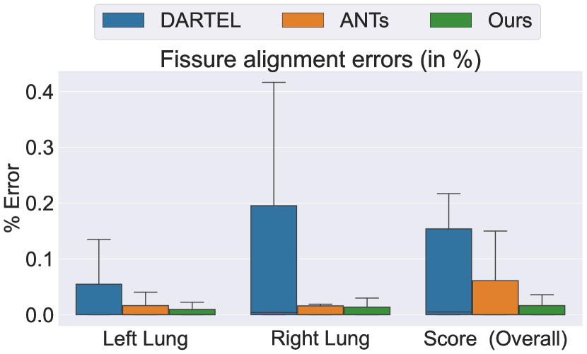
(a) Comparison of fissure alignment error

% Error	DARTEL	ANTs	Ours
Left Lung	3.9983	0.0069	0.0000
Lower Lung	2.7514	0.0177	0.0000
Right Lung	2.4930	0.0107	0.0000
Upper Lung	5.2037	0.0000	0.0000
Score (Overall)	3.0681	0.0088	0.0000

(b) Singularity Errors in %

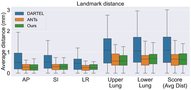
(c) Landmark distance across lung subregions

Method	Left Lung	Right Lung	Score
			(% Error Overall)
Ours	0.0185	0.0254	0.0227
MRF Correspondence Fields	0.0824	0.0211	0.0485
ANTs	0.0249	0.1016	0.0747
Dense Displacement Sampling	0.0578	0.0919	0.0826
ANTs + BSpline	0.0821	0.0848	0.0861
DISCO	0.1256	0.0499	0.0882
VIRNet	0.0834	0.0934	0.0890
Feature-constrained nonlinear registration	0.1210	0.0758	0.1032
Explicit Boundary Alignment	0.1063	0.1246	0.1209
MetaReg	0.1049	0.2224	0.1791

(d) Fissure alignment error on top 10 algorithms in the challenge, averaged on all scan pairs

Figure 3: FireANTs demonstrates state-of-the-art performance on EMPIRE10 lung registration challenge: (a): Lung fissure plates are an important anatomical landmark demarcating lobes within the lung. Fissure alignment errors (in %) denote the percentage of locations near the lung fissure plates that are on the wrong side of the fissure post-registration. Over all 30 scan pairs, our method performs 5$\times$ better than ANTs. (b): Singularity errors defined as percentage of voxels that have a non-diffeomorphic deformation. In the DARTEL baseline, singularities can be introduced for larger deformations due to numerical approximations of the integration. Even for the ANTs baseline, the solutions (deformations) returned are not entirely diffeomorphic. Our method shows much better fissure and landmark alignment ( Fig. 3(a,c),  Fig. S.4, Fig. S.5) with guaranteed diffeomorphic transforms. (c): Landmark distance in mm for selected landmarks. Across different lung subregions, our method shows results at least at par with ANTs, with slightly better average and median results across all regions. (d): Shows the top 10 algorithms for average fissure alignment error in % in the EMPIRE10 challenge. Error metrics are taken from the evaluation server. Other methods perform well on one lung (MRF for right, ANTs for left) but comparatively poorly on the other lung, compared to our method showing both accurate and robustness to both the left and right lung.    X = First,    X = Second,    X = Third best result.

Registration of thoracic CT data is one of the most common areas of research in the medical image registration community. The EMPIRE10 challenge  ¹⁰ is an established benchmark challenge and it provides a platform for in-depth evaluation and fair comparison of available registration algorithms for this application. We discuss more details about the challenge in  Section 4.1. ANTs is, again one of the top performing methods in this challenge. Unlike the brain datasets, ground truth labels for fissure and landmarks are not provided for validation. Therefore, we rely on the evaluation metrics computed in the evaluation server. We compare our method with two powerful baselines (i) ANTs, which optimizes the diffeomorphism directly, and (ii) the DARTEL ⁵³ formulation optimizing a stationary velocity field (SVF), where the diffeomorphism is obtained using an exponential map of the SVF. We first affinely align the binary lung masks of the moving and fixed images using Dice loss ⁶⁵. This is followed by a diffeomorphic registration using the intensity images.

We focus on three evaluation critera of the challenge - (1) fissure alignment errors (in %) denoting the fraction of fissure voxels that are misaligned after registration, (2) landmark distance (in mm), and (3) singularity errors - which is defined as the fraction of the image volume that is warped non-diffeomorphically. Results are summarized in  Fig. 3 which also demonstrates the effect of representation choice for modeling diffeomorphisms. For the same scan pairs and cost functions, the DARTEL baseline performs substantially poorly in terms of fissure alignment, landmark distance and singularities than that of ANTs by three orders of magnitude. Our method has about a 5$\times$ lower error than ANTs on the fissure alignment task, and performs better on 5 out of 6 subregions on the landmark distance alignment task. Moreover, although all methods return deformations that are theoretically diffeomorphic, the SVF representation introduces significant signularity errors (voxels where the deformation is not diffeomorphic) due to discretization errors in the Euler integration. The ANTs baseline also introduces some singularities in its proposed diffeomorphic transform. Our method, on the other hand computes numerically perfect diffeomorphic transforms.

(a) Snapshot of the RnR-ExM leaderboard

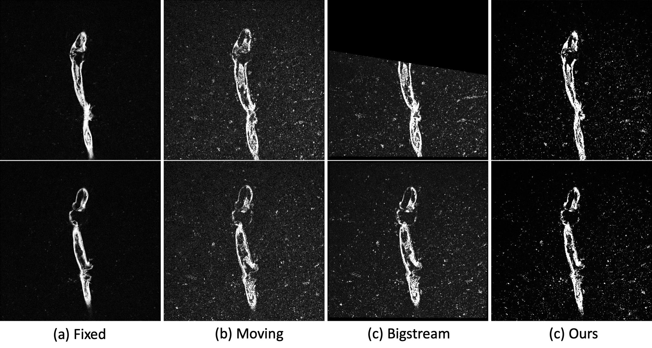
(b) Qualitative comparison of registration of Bigstream and FireANTs

Figure 4: Results on the RnR-ExM mouse dataset: (a): As of March 15, 2024, our method ranks first in the mouse brain registration task, which is the only task in the challenge requiring deformable registration. Our top two successful submissions secure the first and second position, with a 0.361 improvement in Dice score compared to the 3rd ranked submission, which is 0.261 better than the 5th ranked submission (bigstream). Note that among the top 10 submissions, our method has the lowest standard deviation (4.42$\times$ lower than the second best submission) showing the robustness of our model across different microscopy volumes. (b): A qualitative comparison of FireANTs with Bigstream  ⁶², the other top leading method in the challenge. The moving image volumes have substantially more noise than the fixed image volumes, making intensity-based registration difficult. The non-rigid deformation dynamics of the hydrogel are clearly visible, as the moving volume has a thicker boundary than the fixed volume. The bigstream baseline does not capture this dynamics very well - the registered volume looks closer to the moving than the fixed volume. Moreover, the affine registration in Bigstream knocks the boundary slices out of the volume, leading to drop in registration performance. On contrary, our method’s affine and deformable stages are more stable, leading to better registration and avoiding spurious out-of-bound artifacts at the boundary slices.

2.3 Evaluation on high-resolution mouse cortex registration

Expansion Microscopy (ExM) has been a fast-growing imaging technique for super-resolution fluorescence microscopy through tissue expansion ⁶⁶. ExM currently offers 3D nanoscale imaging in tissues with resolution comparable to that of super-resolution microscopy ⁶⁷, which enable morphohological studies of cells and tissues, molecular architecture of diverse multiprotein complexes ⁶⁸, super-resolution imaging of RNA structure and location ⁶⁹. Expansion Microscopy brings forth an unprecedented amount of imaging data with rich structures, but they remain largely unusable by existing registration algorithms due to its scale. Registration in ExM presents a number of challenges, such as repetitive small-scale texture, highly non-linear deformation of the hydrogel, noise in the acquired images, and image size. The Robust Non-rigid Registration Challenge for Expansion Microscopy (RnR-ExM) ⁶⁴ provides a challenging dataset for image registration algorithms. Out of the three species in the challenge, we choose the registration of mouse cortex images, due to its non-linear deformation of the hydrogel and loss of staining intensity. Each volume has a voxel size of 2048$\times$2048$\times$81 with a voxel spacing of 0.1625$\mu$m $\times$ 0.1625$\mu$m $\times$ 0.4$\mu$m for both the fixed and moving images. The volume is 40.5 times bigger than volumes in the brain datasets. To the best of our knowledge, existing solutions ⁶² only consider registering individual chunks of the volumes independently to reduce the time complexity of the registration at the cost of losing information between adjacent chunks of the image, or register highly downsampled versions of the image ⁵² (64$\times$ smaller in-plane resolution).

FireANTs is able to register the volume at native resolution. We perform an affine registration followed by a diffeomorphic registration step. The entire method takes about 2-3 minutes on a single A6000 GPU. As shown in  Fig. 4, our method secures the first place on the leaderboard, with a considerable improvement in the Dice score and a 4.42$\times$ reduction in the standard deviation of the Dice scores compared to the next best method.  Fig. 4 also shows qualitative comparison of our method compared to Bigstream ⁶², the winner of the RnR-ExM challenge. Bigstream only performs an affine registration, leading to inaccurate registration in one of three test volumes, leading to a lower average Dice score and higher variance. Moreover, the affine registration leads to boundary in-plane slices being knocked out of the volume, leading to poor registration. Our method therefore presents a powerful benchmark for accurate and robust deformable image registration.

2.4 Ease of experimentation due to efficient implementation

One of the major contributions of our work is to enable fast and scalable image registration while improving accuracy. In applications like atlas/template building, registration is used in an iterative manner (in the ‘inner loop’) of the optimization. Moreover, modalities such as expansion microscopy enable acquisition of high resolution 3D volumes. Another application that requires fast runtimes is hyperparameter tuning, since different datasets and modalities admit notably different hyperparameters for optimal registration. This calls for an increasing need for fast and scalable registration algorithms. To demonstrate the computational and runtime efficiency of our method, we demonstrate the runtime of our library on the brain and lung datasets. All the experiments for our method are run on a single A6000 GPU, with a batch size of 1 (to avoid amortizing the time over a bigger batch size). For the brain datasets, we run ANTs with the recommended configuration with AMD EPYC 7713 Processor (single thread) and 512GB RAM. For the EMPIRE10 lung dataset, we use the runtimes described in the writeup provided as part of the challenge. A runtime analysis of our method on the brain and EMPIRE10 datasets are shown in Fig. 5.

(a) Timing analysis on four brain MRI datasets.

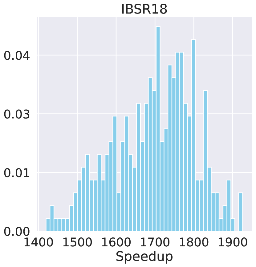
	ANTs	Ours	Speedup
Avg	10380.57	6.11	1701.01
Min	8645.76	5.87	1424.66
Max	11438.96	6.99	1930.78

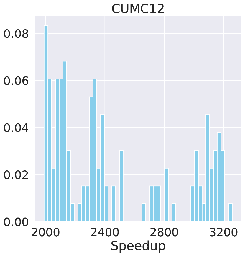
	ANTs	Ours	Speedup
Avg	15497.14	6.30	2475.39
Min	13298.00	5.79	2002.77
Max	18983.44	6.80	3270.91

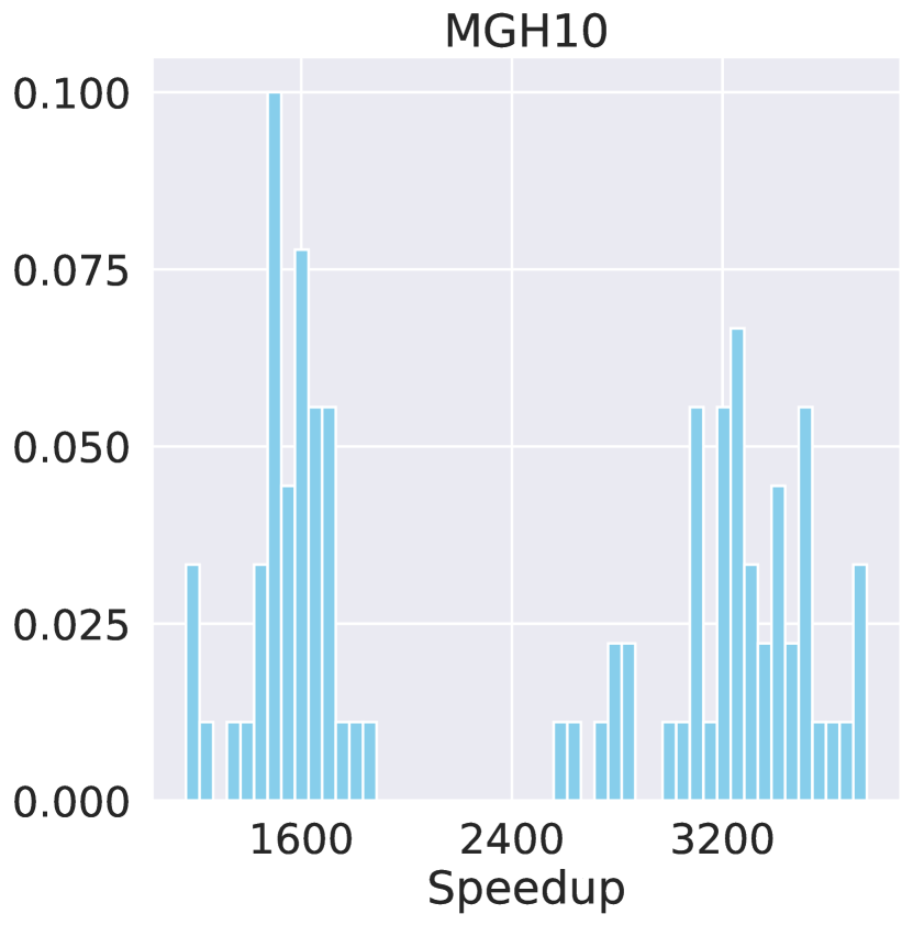
	ANTs	Ours	Speedup
Avg	10558.51	4.25	2486.57
Min	5796.64	3.66	1187.98
Max	15524.08	4.88	3773.99

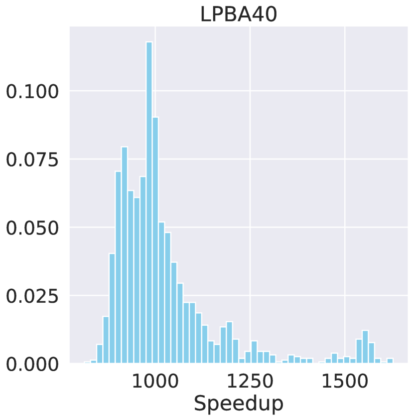
	ANTs	Ours	Speedup
Avg	7273.74	7.02	1036.03
Min	5692.80	6.36	821.20
Max	12068.08	7.66	1635.29

(b) Timing analysis on EMPIRE10 dataset

	ANTs	DARTEL	Ours	Speedup (ANTs)	Speedup (DARTEL)
Avg	6hr 14m	7hr 16m	0m 39s	562.67	663.77
Min	0h 55m	1h 8m	0m 9s	320.74	315.23
Max	12h 41m	10h 11m	1m 5s	1231.27	796.51

Figure 5: Timing analysis of our library: We compare the runtime of our implementation with the ANTs library. (a) shows distribution of speedup (runtime of ANTs divided by runtime of our method) and statistics of runtimes (in seconds) for the four brain MRI datasets. For all datasets, our implementation runs a minimum of two orders of magnitudes faster, making it suitable for hyperparameter search algorithms, and larger datasets. Table (b) shows the runtime of ANTs, DARTEL and our implementation on the EMPIRE10 challenge data. The first three colums show the actual runtime of the methods, followed by the speedup obtained by our method when compared to ANTs and DARTEL. Note that our method runs a minimum of 320 times faster than ANTs, saving a substantial amount of time, at no loss in registration quality.

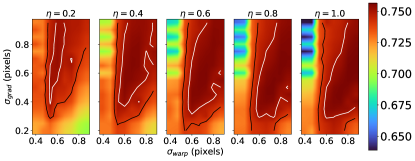
(a) Grid search on LPBA40 dataset

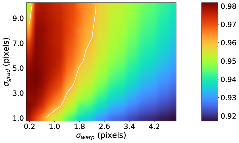
(b) Grid search on the EMPIRE10 dataset, with Dice score

Figure 6: Feasibility of hyperparameter searches on LPBA40 and EMPIRE10 datasets: The speed of FireANTs makes hyperparameter studies like these feasible, which ANTs would take years to complete. (a): We perform a hyperparameter grid search on three hyperparameters of interest - smoothing kernel for the warp field ($\sigma_{\text{warp}}$) in pixels, smoothing kernel for the gradient of warp field ($\sigma_{\text{grad}}$) in pixels and learning rate $\eta$. The metric to optimize in this case is the target overlap. For the LPBA40 dataset, we perform a hyperparameter sweep over 640 configurations in 40 hours with 8 A6000 GPUs. A corresponding hyperparameter sweep with 8 concurrent jobs with each job consuming 8 CPUs would take $\sim$3.6 years to complete. The white contour representing the level set for target overlap = 0.75, and the black contour representing the level set for target overlap of 0.74 show the robustness of our method to hyperparameters - performance is not brittle or sensitive to choice of hyperparameters. (b): Hyperparameter grid search on the EMPIRE10 dataset over $\sigma_{\text{warp}}$ and $\sigma_{\text{grad}}$ parameters (456 configurations), with a fixed learning rate of $\eta=0.25$. The metric to optimize is the Dice score of the provided binary lung mask. This sweep takes about 12.37 hours on 8 GPUs, whereas a corresponding sweep would take 296 days for ANTs and 345 days for DARTEL (more in Fig. 5). The white contour corresponds to the level set for Dice score = 0.96, showing both a huge spectrum of parameters that achieve high Dice scores, and low sensitivity of the method to choice of hyperparameters.

For the EMPIRE10 dataset, our method reduces the runtime from 1 to 12 hours for a single scan pair to under a minute. We compare our method with both ANTs and DARTEL implementations. Since the exponential map requires a few integration steps for each iteration, this variant is even slower than ANTs. Our method enjoys a minimum of more than 300$\times$ speedup over ANTs. On the brain datasets, our method achieves a consistent speedup of 3 orders of magnitude. This happens due to a better choice of hyperparameters compared to the baseline, faster convergence due to the adaptive optimization, and better memory and compute utilization by cuDNN implementations. These improvements in runtime occur while also providing at par, or superior results (Fig. 2, 3, Extended Data S.4, S.5).

2.4.1 Fast hyperparameter tuning using FireANTs

In optimization toolkits such as ANTs, several hyperparameters are key to high quality registration. Some of these hyperparameters are the window size for the similarity metric Cross-Correlation or bin size for Mutual Information. In our experience, the Gaussian smoothing kernel $\sigma_{\text{grad}}$ for the gradient of the warp field are two of the most important parameters for diffeomorphic registration. The optimal values of these hyperparameters vary by image modality, intensity profile, noise and resolution. Typically, these values are provided by some combination of expertise of domain experts and trial-and-error. However, non experts may not be able to adopt these parameters in different domains or novel acquisition settings. Recently, techniques such as hyperparameter tuning have become popular, especially in deep learning. In the case of registration, hyperparameter search can be performed by considering some form of label/landmark overlap measure between images in a validation set. We demonstrate the stability and runtime efficiency of our method using two experiments : (1) Owing to the fast runtimes of our implementation, we show that hyperparameter tuning is now feasible for different datasets. The optimal set of hyperparameters is dependent on the dataset and image statistics, as shown in the LPBA40 and EMPIRE10 datasets; (2) within a particular dataset, the sensitivity of our method around the optimal hyperparameters is very low, demonstrating the robustness and reliability of our method.

We choose the LPBA40 dataset among the 4 brain datasets due to its larger size (40$\times$39 = 1560 pairs). We choose three parameters to search over : the learning rate ($\eta$), and the gaussian smoothing parameters $\sigma_{\text{warp}},\sigma_{\text{grad}}$. We use the Ray library (https://docs.ray.io/) to perform a hyperparameter tuning using grid search. For the LPBA40 dataset, a grid search over three parameters (shown in  Fig. 6) takes about 40.4 hours with 8 parallel jobs. On the contrary, ANTs would require around 3.6 years to complete the same grid search, with 8 threads allocated to each job and 8 parallel jobs. This makes hyperparameter search for a unknown modality computationally feasible.  6(a) shows a dense red region suggesting the final target overlap is not sensitive to the choice of hyperparameters. Specifically, the maximum target overlap is 0.7565 and 58.4% of these configurations have an average target overlap of $\geq$ 0.74. This is demonstrated in  Fig. 6 (top) by the white contour line denoting the level set for target overlap = 0.75, and the black contour line denoting the level set for target overlap of 0.74. The target overlap is quite insensitive to the learning rate ($\geq 0.4$) showing that our algorithm achieves fast convergence with a smaller learning rate. On the EMPIRE10 dataset, we fix the learning rate and perform a similar hyperparamter search over two parameters, the Gaussian smoothing parameters $\sigma_{\text{warp}},\sigma_{\text{grad}}$. We use the average Dice score between the fixed and moving lung mask to choose the optimal hyperparameters. FireANTs can perform a full grid search over 456 configurations on the EMPIRE10 dataset in 12.37 hours with 8 A6000 GPUs, while it takes SyN 10.031 days to run over a single configuration, or equivalently around 296 days for the entire grid search. Normalizing for 8 concurrent jobs and 456 configurations, it would take ANTs about 296 days, and DARTEL about 345 days. This shows that our method and accompanying implementation can now make hyperparameter search for 3D image registration studies feasible.

3 Discussion

We present FireANTs, a powerful and general purpose multi-scale registration algorithm. Our method performs registration by generalizing the concept of first-order adaptive optimization schemes for optimizing parameters in the Euclidean space, to diffeomorphisms. This is highly non-trivial because diffeomorphisms are typically implemented as an image grid proportional to the size of the fixed image, and are optimized in a multi-scale manner to capture large deformations ^{32, 60, 53} leading to changing grid size over the course of optimization. Our method also avoids a computationally expensive parallel transport step for diffeomorphisms by solving a modified instance of registration at each time step. Our method achieves consistent improvements in performance over state-of-the-art optimization-based registration algorithms like ANTs, DARTEL, SynthMorph and Bigstream. This improvement is shown across six datasets with a spectrum of anatomies (in-vivo human brain, human and ovine lungs, mouse cortex), contrast, image volume sizes (ranging from 196 up to 2048 voxels per dimension), and modalities (MRI, CT, microscopy). A key advantage of our method is that we do not tradeoff any of accuracy, speed or robustness for the others, thus being a powerful registration algorithm.

Our method shows consistent improvements and robust performance on four public brain MRI datasets. Many classical image registration methods have been developed for neuroimaging studies ^{60, 53, 38, 70} and registration still remains a crucial component in brain mapping ^{71, 72}. FireANTs’ consistent improvement in performance can be attributed to the quasi-second-order update which normalizes the varying curvature of the per-pixel gradient, leading to faster convergence. This performance is consistent across metrics ( Fig. 2) and anatomical structures ( Fig. S.1). With acquisition of larger datasets ⁷³ and high-resolution imaging ⁷⁴, fast and accurate registration runtimes become imperative to enable large-scale studies. Our performance comes with a reduction of runtime of up to three orders of magnitude.

We also demonstrate competitive performance in the EMPIRE10 challenge, widely regarded as a comprehensive evaluation of registration algorithms ^{63, 75}. Unlike the brain imaging datasets, the EMPIRE10 dataset contains images with large deformations, anisotropic image spacings and sizes, and thin structures like airways and pulmonary fissures which are hard to align based on image intensity alone. These image volumes are typically much larger than what deep learning methods can currently handle at native resolution ^{75, 52, 46}. FireANTs performs much better registration in terms of landmark, fissure alignment and singularities, while being two orders of magnitude faster. This experiment also calls attention to a much overlooked detail - the performance gap due to choice of representation of diffeomorphisms (direct Riemannian optimization versus exponential map). We show that direct Riemannian optimization is preferable to exponential maps, both in FireANTs and in baselines (ANTs versus DARTEL). This is because computing the exponential map is expensive for diffeomorphisms, the number of iterations can be large for large deformations ⁵³. For example, in Fig. 5(a), the exponential map representation (DARTEL) takes substantially longer to run, compared to ANTS. Shooting methods modify the velocity field at each iteration and tend to be sensitive to hyper-parameter choices. For example, in Fig. 3 the results for shooting methods are substantially worse those for methods that optimize the transformation directly. We also observe this for the LPBA40 dataset in Fig. S.6, where over a wide range of hyperparameter choices, the shooting method consistently under-performed.

Our method is consistently 300–2000$\times$ faster, is robust to choice of hyperparameters, allowing users to utilize principled hyperparameter search algorithms for novel applications or modalities. This opens up many other avenues in registration, including modalities such as microscopy, ex-vivo imaging where advanced imaging techniques have led to ultra high resolution data acquisition protocols. Registration algorithms are crucial to subsequent downstream tasks in these studies, it is therefore imperative for registration algorithms to be accurate and scale with the data as well. Our method showcases this on the RnR-ExM mouse cortex dataset, where our method performs the best overall in a 2-3 minute runtime on a single GPU. Our method and accompanying implementation is a step towards this avenue, making advanced registration algorithms fast and accessible.

In summary, FireANTs is a powerful and general purpose multi-scale registration algorithm and sets a new state-of-the-art benchmark. We propose to leverge the accurate, robust and fast library to speed up registration workflows for modalities like microscopy and ex-vivo imaging (humans, mice, C. Elegans, etc.), where imaging resolutions are large and algorithms are bottlenecked by scalability.

4 Methods

Given $d$-dimensional images $I:\Omega\to\mathbb{R}^{d}$ and $I^{\prime}:\Omega\to\mathbb{R}^{d}$ where the domain $\Omega$ is a compact subset of $\mathbb{R}^{2}$ or $\mathbb{R}^{3}$, image registration is formulated as an optimization problem to find a transformation $\varphi$ that warps $I^{\prime}$ to $I$. The transformation can belong to a group, say $G$, whose elements $g\in G$ act on the image by transforming the domain as $(I\circ g)(x)=I(g(x))$ for all $x\in\Omega$. The registration problem solves for

$$\varphi^{*}=\operatorname*{\text{argmin}}_{\varphi\in G}L(\varphi)\doteq C(I,I^{\prime}\circ\varphi)+R(\varphi)$$ (1)

where $C$ is a cost function, e.g., that matches the pixel intensities of the warped image with those of the fixed image, or local normalized cross-correlation or mutual information across image patches. There are many types of regularizers $R$ used in practice, e.g., total variation, elastic regularization ³³, enforcing the transformation to be invertible ³⁴, or volume-preserving ⁷⁶ using constraints on the determinant of the Jacobian of $\varphi$, etc. If, in addition to the pixel intensities, one also has access to label maps or different anatomical regions marked with correspondences across the two images, the cost $C$ can be modified to ensure that $\varphi$ transforms these label maps or landmarks appropriately.

We perform registration over the group of diffeomorphisms $G=\text{Diff}(\Omega)$; a diffeomorphism is a smooth and invertible map with a corresponding differentiable inverse map ^{77, 78, 79}. It is useful to note that unlike rigid or affine transforms that have a fixed number of parameters, the number of parameters in a diffeomorphism scales with the size of the domain. When groups of transformations on continuous domains are endowed with a differentiable structure, they are called Lie groups. Lie groups equipped with a Riemannian metric are Riemannian manifolds.

To summarize, there are three key parts of registration methods: the objective, the group $G$, and the optimization algorithm. Our work focuses on developing new optimization algorithms.

Euclidean gradient descent using the Lie algebra in shooting methods

Each Lie group has a corresponding Lie algebra $\mathfrak{g}$ which is the tangent space at identity. This creates a one-to-one correspondence between elements of the group $g\in G$ and elements of its Lie algebra $v\in\mathfrak{g}$ given by the exponential map

$$\exp:\mathfrak{g}\to G;$$

effectively to reach $g=\exp(v)\text{Id}$ from identity $\text{Id}\in G$, the exponential map says that we have to move along $v$ for unit time. Exponential maps for many groups can be computed analytically, e.g., Rodrigues transformation for rotations, Jordan-Chevalley decomposition ⁸⁰, or the Cayley Hamilton theorem ⁸¹ for matrices. For diffeomorphisms, the Lie algebra is the space of all smooth velocity fields $v:\Omega\to\mathbb{R}^{d}$. There exist iterative methods to approximate the exponential map called the scaling-and-squaring approach ^{53, 46} which uses the identity

$$\varphi=\exp(v)=\lim_{N\to\infty}\left(\text{Id}+\frac{v}{N}\right)^{N}$$

to define a recursion by choosing $N$ to be a large power of 2, i.e. $N=2^{M}$ as

$$\varphi^{(1/2^{M})} =x+v(x)/2^{M}$$

$$\varphi^{(1/2^{k})} =\varphi^{(1/2^{(k+1)})}\circ\varphi^{(1/2^{(k+1)})}\quad\quad\forall k\in\{0,1\ldots,M-1\};$$

By virtue of the exponential map, we can solve the registration problem of finding $\varphi\in G$ by directly optimizing over the Lie algebra $v$. This is because the Lie algebra is a vector space and we can perform, for example, standard Euclidean gradient descent for registration ^{82, 83, 84}. Such methods are called stationary velocity field or shooting methods. At each iteration, one uses the exponential map to get the transformation $\varphi$ from the velocity field $v$, computes the gradient of the registration objective with respect to $\varphi$, pulls back this gradient into the tangent space where $v$ lies

$$\nabla_{v}L=\partialderivative{\varphi}{v}\nabla_{\varphi}L$$

and finally makes an update to $v$. Traditional methods like DARTEL ⁵³ implement this approach. This is also very commonly used by deep learning methods for registration ^{46, 8, 42} due to its simplicity. Geodesic shooting methods are more sophisticated implementations of this approach where the diffeomorphism $\varphi$ is the solution of a time-dependent velocity which follows the geodesic equation; the geodesic is completely determined by the initial velocity $v_{0}\in\mathfrak{g}$.

Riemannian gradient descent

Solving the registration problem directly on the space of diffeomorphisms avoids repeated computations to and fro via the exponential map. The downside however is that one now has to explicitly account for the curvature and tangent spaces of the manifold. The updates for Riemannian gradient descent ⁵⁹ at the $t^{\text{th}}$ iteration are

$$\varphi_{t+1} =\exp_{\varphi_{t}}\left(-\eta\ \text{Proj}_{\varphi_{t}}(\nabla_{\varphi}L)\right)$$ (2)

$$\nabla_{\varphi}L =\mathbf{g}^{-1}_{\varphi_{t}}\frac{\partial L}{\partial\varphi},$$

where one pulls back the Euclidean gradient $\frac{\partial L}{\partial\varphi}$ onto the manifold using the inverse metric tensor $\mathbf{g}$ (which makes the gradient invariant to the parameterization of the manifold of diffeomorphisms) before projecting it to the tangent space using $\text{Proj}_{\varphi_{t}}$. Since the tangent space is a local first-order approximation of the manifold’s surface, we can move along this descent direction by a step-size $\eta$ and compute the updated diffeomorphism $\varphi_{t+1}$, represented as the exponential map from $\varphi_{t}$ computed in the direction of $-\text{Proj}_{\varphi_{t}}(\nabla_{\varphi}L)$. In our work, we take advantage of a few key properties of diffeomorphisms. (a) If the step-size $\eta$ is small, the exponential map can be well approximated with a retraction map, which is quick to compute  ^{44, 45}. (b) The metric tensor is the Jacobian of the diffeomorphism $\varphi_{t}$ ^{79, 40} which can be approximated with finite differences. (c) The tangent space is the set of all $C^{\infty}$ velocity fields, which is the same as the ambient space of the diffeomorphisms and therefore we can omit the projection step. We also implement a stochastic variant of Riemannian gradient descent whereby we only update the diffeomorphism on a subset of the image domain; convergence properties of this algorithm can be studied ⁵⁷.

For high-dimensional groups like diffeomorphisms, optimizing the transformation directly on the manifold is preferable to optimizing on the Lie algebra. We noticed this empirically in a number of instances. In Fig. 3, the greedy SyN method (which performs Riemannian optimization) outperforms the Lie algebra variant (DARTEL) significantly, runs much faster on average (computation of the exponential map and its derivative adds additional time and memory overhead), and results in substantially fewer singularities in the velocity field. Similar observations may be made for EMPIRE10 dataset in the ANTs baseline. In  Fig. S.6 we observed the across a large variety of hyper-parameters (obtained via grid search), Riemannian gradient descent leads to better target overlap compared to the Lie algebra variant on the LPBA40 dataset.

Adaptive Riemannian optimization for diffeomorphisms

Adaptive optimization algorithms such as RMSProp ⁵⁴, Adagrad ⁵⁶ and Adam ⁵⁵ have become popular because they can handle poorly conditioned optimization problems in deep learning. Variants for optimization on low-dimensional Riemannian manifold exist ^{57, 85, 86, 58}. Diffeomorphisms are a high-dimensional group (e.g., the size of velocity field scales with that of the domain). Also, often the number of parameters (e.g., size of the image) in these methods is fixed which makes it difficult to run them on diverse datasets and modalities. We develop a multi-scale ^{60, 87, 45, 53} approach to optimization on Riemannian manifolds that can adapt the updates to the curvature of the manifold and that work for pairs of images of different sizes.

Adaptive optimization methods, in Euclidean space, typically maintain a moving average of past gradients (momentum) and an approximation of the Hessian (which allows approximate second-order updates). The Hessian is generally expensive to compute and store, and therefore only diagonal elements are sometimes computed; one may resort to further approximations (like Adam does) and maintain a running average of the element-wise squared gradients (we will call this the “curvature vector”). Both the momentum and the curvature vector can be thought of as vectors in the tangent space. For Euclidean manifolds, the tangent space is the same as the manifold and it is easy to compute the modified descent direction by transporting the momentum and the curvature vectors along a straight line; in Euclidean space such transport does not change the magnitude or direction of a vector. On curved manifolds, parallel transport generalizes the notion of transporting a vector $v$ from the paths connecting a point $\varphi$ to another $\varphi^{\prime}$. And unlike Euclidean space, parallel transport depends upon the path between the two points. It is expensive to compute parallel transport for groups such as diffeomorphisms. This makes it difficult and expensive to implement adaptive optimization methods.

We can work around the above issue using a result of Younes et al. ⁷⁹ on computing the differentials at any transformation $\varphi$ using the differential at identity Id. Let us first rewrite Eq. 2 in a slightly different notation. The Eulerian differential $\bar{\partial}L(\varphi)$ is a linear map (also called a linear form) from vector fields on $\Omega$ to real numbers, and denotes the change in $L$ when $\varphi$ is changed along a velocity field $v$

$$\left(\bar{\partial}L(\varphi)\mid v\right)=\partial_{\epsilon}L(\varphi+\epsilon(v\circ\varphi))|_{\epsilon=0}.$$

Much like standard gradient descent in Euclidean space, iterative updates to the diffeomorphism $\varphi$ using the Eulerian differential minimize the objective $L$. We have

$$\left(\bar{\partial}L(\varphi)\mid v\right)=\left(\frac{\delta L}{\delta\varphi}\mid v\circ\varphi\right),$$

for any velocity field $v$. This is a direct correspondence between the Eulerian differential that performs Riemannian gradient descent in Eq. 2 on the left-hand side and the conventional derivative that can be calculated analytically on the right-hand side. Exploiting this correspondence for optimization requires computing $v\circ\varphi$ each time. But Younes et al.show in Section 10.2 of their book ⁷⁹ that:

$$\left(\bar{\partial}L(\varphi;\ I,I^{\prime})\mid v\right)=\left(\bar{\partial}L(\text{Id};\ I,I^{\prime}\circ\varphi)\mid v\right).$$ (3)

This allows us to represent the Riemannian gradient at arbitrary $\varphi$ (left) in terms of the gradient at $\varphi=\text{Id}$ calculated for the deformed image $I^{\prime}\circ\varphi$ (right). In simpler words, we can pretend as if the optimization algorithm always works at identity Id at every iteration if we match to a warped image $I^{\prime}\circ\varphi_{t}$. When Riemannian gradient descent is implemented like this, gradients, momentum and curvature vector lie in the tangent space at identity for all iterations, and calculating the gradient descent update is therefore identical to that of the Euclidean case. Parallel transport is not required. The Riemannian metric tensor $\mathbf{g}_{\varphi_{t}}$ is also the outer product of the Jacobian of the diffeomorphism at identity; this is identity. We therefore do not need to pullback the gradient in Eq. 2 on the manifold. This is a very useful technique that eliminates a number of computationally expensive steps. We should emphasize that it is mathematically rigorous and does not result from any approximations. We illustrate this procedure in  Fig. S.3(a).

Interpolation strategies for multi-scale registration

Classical approaches to deformable image registration is performed in a multi-scale manner. Specifically, an image pyramid is constructed from the fixed and moving images by downsampling them at different scales, usually in increasing powers of two. Optimization is performed at the coarsest scale first, and the resulting transformation at each level is used to initialize the optimization at the next finer scale. Specifically, for the fixed image $I$ and the moving image $I^{\prime}$ and $K$ levels, let the downsampled versions be $\{I_{k}\}_{k=1}^{K}$ and $\{I^{\prime}_{k}\}_{k=1}^{K}$, where $k$ is the scale index from coarsest to finest. At the $k$-th scale, the transformation $\varphi_{k}$ is optimized as

$$\varphi_{k}^{*}=\operatorname*{\text{argmin}}_{\varphi_{k}\in G}L(I_{k},I^{\prime}_{k}\circ\varphi_{k})$$

where $\varphi_{k}$ is initialized as

$$\varphi_{k}=\begin{cases}\text{Id}&\text{if }k=1\\ \text{Upsample}(\varphi_{k-1})&\text{otherwise}\end{cases}$$

Unlike existing gradient descent based approaches, our Riemannian adaptive optimizer also contains state variables $m_{k}$ corresponding to the momentum and $\nu_{k}$ corresponding to the EMA of squared gradient, at the same scale as $\varphi_{k}$, which require upsampling as well.

Unlike upsampling images, upsampling warp fields and their corresponding optimizer state variables requires careful consideration of the interpolation strategy. Bicubic interpolation is a commonly used strategy for upsampling images to preserve smoothness and avoid aliasing. However, bicubic interpolation of the warp field can lead to overshooting, leading to introducing singularities in the upsampled displacement field when there existed none in the original displacement field. In contrast, bilinear or trilinear interpolation does not lead to overshooting, and therefore diffeomorphism of the upsampled displacement is guaranteed, if the original displacement is diffeomorphic.

We demonstrate this using a simple 2D warp field in  Fig. S.3(b). On the left, we consider a warp field created by nonlinear shear forces. This warp field does not contain any tears or folds - and is diffeomorphic. We upsample this warp field using bicubic interpolation (top) and bilinear interpolation (bottom). We also plot a heatmap of the negative of the determinant of the Jacobian of the upsampled warp, with a contour representing the zero level set. Qualitatively, bicubic interpolation introduces noticable folds in the warping field, leading to non-diffeomorphisms in the upsampled warp field. The heatmap shows a significant portion of the upsampled warp field has a negative determinant, indicating non-invertibility. On the other hand, bilinear interpolation looks blocky but preserves diffeomorphism everywhere, as also quantitatively verified by the absence of a zero level set in the heatmap.

Modular software implementation to enable effective experimentation

Registration is a key part of many data processing pipelines in the clinical literature. Our software implementation is designed to be extremely flexible, e.g., it implements a number of existing registration methods using our techniques, modular, e.g., the user can choose different group representations (rigid or affine transforms, diffeomorphisms), objective functions, optimization algorithms, loss functions, and regularizers. Users can also stack the same class of transformations, but with different cost functions. For example, they can fit an affine transform using label maps and Dice loss, and use the resultant affine matrix as initialization to fit another affine transform using the cross-correlation registration objective. This enables seamless tinkering and real-time investigation of the data. Deformations can also be composed in increasing order of complexity (rigid $\to$ affine $\to$ diffeomorphisms), thereby avoiding multiple resampling and subsequent resampling artifacts. We have developed a simple interface to implement custom cost functions, which may be required for different problem domains, with ease; these custom cost functions can be used for any of the registration algorithms out-of-the-box. Our implementation can handle images of different sizes, anisotropic spacing, without the need for resampling into a consistent physical spacing or voxel sizes. All algorithms also support multi-scale optimization (even with fractional scales) and convergence monitors for early-stopping.

Our software is implemented completely using default primitives in PyTorch. All code and example scripts is available at https://github.com/rohitrango/fireants.

4.1 Experiment Setup

Klein et al. brain mapping challenge  ⁵

Brain mapping requires a common coordinate reference frame to consistently and accurately communicate the spatial relationships within the data. Automatically determining anatomical correspondence is almost universally done by registering brains to one another or to a template. Klein et al.evaluate a suite of fully automated nonlinear deformation algorithms applied to human brain image registration. A natural way to evaluate whether two images are in a common coordinate frame is to evaluate the accuracy of overlap of gross morphological structures (gryi, sulci, subcortical regions for example). The evaluation considers a total of four T1-weighted brain datasets with different whole-brain labelling protocols, eight different evaluation measures and three independent analysis methods. The paper evaluates 14 nonlinear registration algorithms with different parameterizations and assupmtions about the deformation field, and different regularizations.

Brain image data and their corresponding labels for 80 normal subjects were acquired from four different datasets. The LPBA40 dataset contains 40 brain images and their labels to construct the LONI Probabilistic Brain Atlas (LPBA40). All volumes were skull-stripped, and aligned to the MNI305 atlas  ⁸⁸ using rigid-body transformation to correct for head tilt. For all these subjects, 56 structures were manually labelled and bias-corrected using the BrainSuite software. The IBSR18 dataset contains brain images acquired at different laboraties through the Internet Brain Segmentation Repository. The T1-weighted images were rotated to be in Talairach alignment and bias-corrected. Manual labelling is performed resulting in 84 labeled regions. For the CUMC12 dataset, 12 subjects were scanned at Columbia University Medical Center on a 1.5T GE scanner. Images were resliced, rotated, segmented and manually labeled, leading to 128 labeled regions. Finally, the MGH10 dataset contains 10 subjects who were scanned at the MGH/MIT/HMS Athinoula A. Martinos Center using a 3T Siemens scanner. The data is bias-corrected, affine-registered to the MNI152 template, and segmented. Finally the images were manually labeled, leading to 74 labeled regions. All datasets have a volume of $256\times 256\times\{128,124\}$ voxels with varying amounts of anisotropic voxel spacing, ranging from $0.84\times 0.84\times 1.5$mm to $1\times 1\times 1.33$mm.

ANTs was one of the top performing methods for this challenge, performing well robustly across all four datasets. The method considers measures of volume and surface overlap, volume similarity, and distance measures to evaluate the alignment of anatomical regions. Given a source label map ${S}_{r}$ and target label map ${T}_{r}$ and a cardinality operator $|.|$, we consider the following overlap measures. The first measure ‘target overlap’, defined as the overlap between the source and target divided by the target.

$$TO_{r}=\frac{|{S}_{r}\cap{T}_{r}|}{|{T}_{r}|}$$ (4)

Target overlap is a measure of sensitivity, and the original evaluation ⁵ considers the aggregate total overlap as follows

$$TO_{Klein}=\frac{\sum_{r}|{S}_{r}\cap{T}_{r}|}{\sum_{r}|{T}_{r}|}$$ (5)

However, we notice that this measure of overlap is biased towards larger anatomical structures, since both the numerator $\sum_{r}|{S}_{r}\cap{T}_{r}|$ and denominator $\sum_{r}|{T}_{r}|$ sums are dominated by regions with larger number of pixels. To normalize for this bias, we also consider a target overlap that is simply the average of region-wise target overlap.

$$TO=\frac{1}{N_{r}}\sum_{r}TO_{r}$$ (6)

We also consider a second measure, called mean overlap (MO), more popularly known as the Dice coefficient or Dice score. It is defined as the intersection over mean of the two volumes. Similar to target overlap, we consider two aggregates of the mean overlap over regions:

$$MO_{r} =2\frac{|{S}_{r}\cap{T}_{r}|}{|{S}_{r}|+|{T}_{r}|}$$ (7)

$$MO_{Klein} =2\frac{\sum_{r}|{S}_{r}\cap{T}_{r}|}{\sum_{r}(|{S}_{r}|+|{T}_{r}|)}$$ (8)

$$MO =\frac{1}{N_{r}}\sum_{r}MO_{r}$$ (9)

Klein et al.⁵ also propose a ‘Union Overlap’ metric which is a monotonic function of the Dice score. Therefore, we do not use this in our evaluation. To complement the above agreement measures, we also compute false negatives (FN), false positives (FP), and volume similarity (VS) coefficient for anatomical region $r$:

$$FN_{r}=\frac{|{T}_{r}\backslash{S}_{r}|}{|{T}_{r}|},\quad FP_{r}=\frac{|{S}_{r}\backslash{T}_{r}|}{|{S}_{r}|},\quad VS_{r}=2\frac{|{S}_{r}|-|{T}_{r}|}{|{S}_{r}|+|{T}_{r}|}$$ (10)

Similar to the overlap metrics, we compute the aggregates as in the original evaluation denoted by $FN_{Klein},FP_{Klein},VS_{Klein}$ and average over regions denoted simply by FN, FP, VS. This leads to a total of 10 aggregate metrics that we use to compare our method with 4 baselines - ANTs, Demons, VoxelMorph and SynthMorph.

EMPIRE10 challenge  ¹⁰

Alignment of thoracic CT images, especially the lung and its internal structures is a challenging task, owing to the highly deformable nature of the lungs. Pulmonary registration is clinically useful, for example registering temporally distinct breathhold scans make visual comparison of these scans easier and less error prone. Registering inspiration and expiration scans can also be used to model or understand the biomechanics of lung expansion. Registration of temporally spaced breathhold scans can help in tracking disease progression, or registration between inspiration and expiration scans can enable improved monitoring of airflow and pulmonary function. Murphy et al.propose the Evaluation of Methods for Pulmonary Image REgistration 2010 (EMPIRE10) challenge to provide a platform for a comprehensive evaluation and fair comparison of registration algorithms for the task of CT lung registration. The dataset consists of 30 scan pairs including inspiration-expiration scans, breathhold scans over time, scans from 4D data, ovine data, contrast-noncontrast, and artificially warped scan pairs. The ovine data was acquired where breathing was controlled, and metallic markers were surgically implanted to provide landmark annotations, followed by a hole-filling algorithm to disguise the markers so that registration algorithms cannot use this artificial information. Artificially warped scan pairs also provide ground truth correspondences for landmarks and lung boundaries. The challenge provides a broad range of data complexity, voxel sizes and image acquisition differences. In this challenge, only intrapatient registration is considered, and lungs and lung fissures were segmented using an automated method, and altered manually wherever necessary. The challenge only provides scan pairs and binary lung masks. All the other data (fissures and landmarks) are withheld for evaluation. All the scan pairs have varying spatial and physical resolutions, are acquired over a varying set of imaging configurations. This calls for a registration algorithm that is agnostic to any assumptions about anisotropy of image resolution, both physical and voxel. We use the evaluation provided by the challenge, and compare the fissure alignment, landmark alignment, and singularity of registration. More details about the evaluation can be found in  ¹⁰. We compare our method with ANTs which performs direct gradient descent updates and DARTEL which optimizes a stationary velocity field using the metrics reported in the evaluation server.

RnR ExM mouse dataset  ⁶⁴

Expansion microscopy (ExM) is a fast-growing imaging technique for super-resolution fluorescence microscopy. It is therefore critical to robustly register high-resolution 3D microscopy volumes from different sets of staining. The RnR-ExM challenge checks the ability to perform non linear deformable registration on images that have a very high voxel resolution. The challenge releases 24 pairs of 3D image volumes from three different species. Out of the three species (mouse brain, C. elegans, zebrafish), the mouse brain dataset is the only dataset with non-trivial non-linear deformations, and the other datasets mostly require a rigid registration. The mouse dataset has non-rigid deformation of the hydrogel and loss of staining intensity. Deformation of the hydrogel occurs because the sample sits for multiple days and at a low temperature between staining rounds. This calls for a cost function like cross-correlation which is sufficiently robust to the change in intensity as long as the structures are visible. The voxel size of each image volume is 2048x2048x81 and the voxel spacing is 0.1625$\mu$m x 0.1625$\mu$m x 0.4$\mu$m. The challenge reports the average Dice score for the test set and also reports individual dice scores.

Appendix A Extended Data

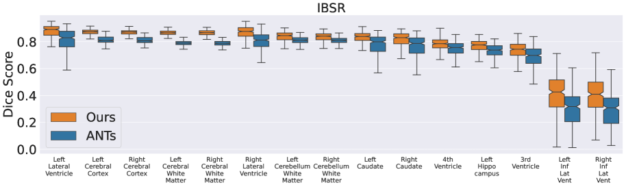
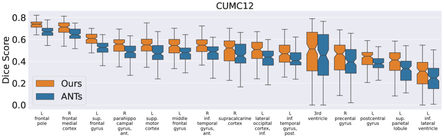
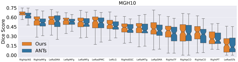
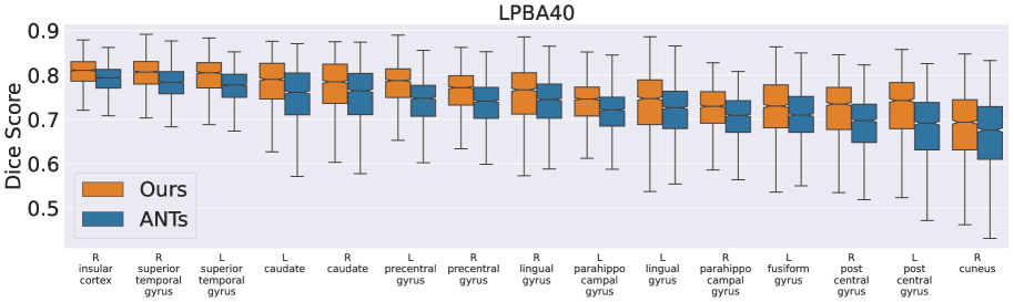
Figure S.1: Regionwise target overlap on the brain MRI datasets: We further evaluate regionwise overlap scores by sampling 15 regions from each dataset, and comparing their distribution using our method and ANTs. Our method has a much higher median score, and better interquartile ranges across regions, demonstrating both accuracy and robustness.

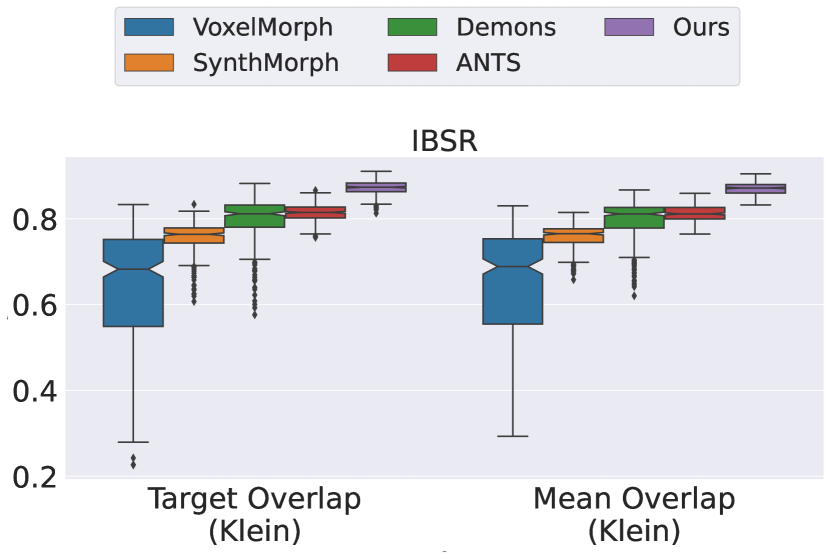
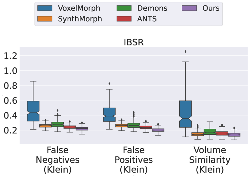
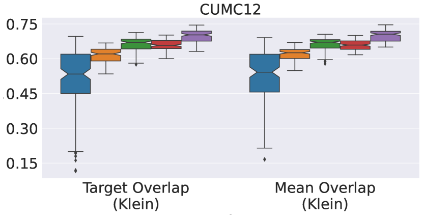
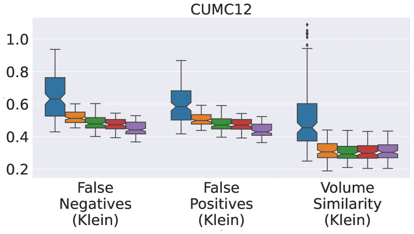
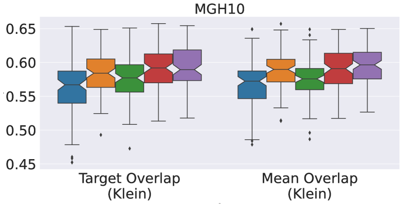
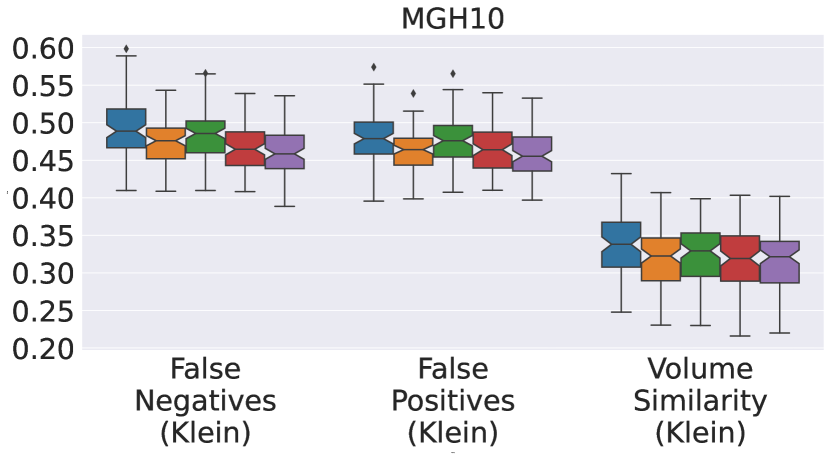
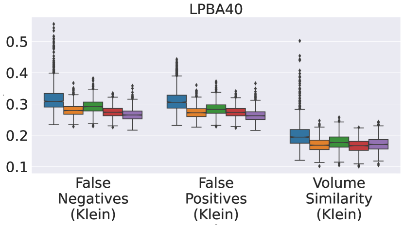
Figure S.2: Comparison of our method with ANTs on 4 MRI brain datasets: Registration quality is validated by measuring volume overlap of label maps between the fixed and warped label maps. (a): For anatomical region $r$, warped (binary) label map ${S}_{r}$ and fixed label map ${T}_{r}$, target and mean overlap are defined as $|{S}_{r}\cap{T}_{r}|/|{T}_{r}|$ and $2|{S}_{r}\cap{T}_{r}|/(|{S}_{r}|+|{T}_{r}|)$. We define the aggregate target overlap over all anatomical regions as $\sum_{r}(|{S}_{r}\cap{T}_{r}|/|{T}_{r}|)$ and Klein et al. ⁵ define it as $(\sum_{r}|{S}_{r}\cap{T}_{r}|)/(\sum_{r}|{T}_{r}|)$, likewise for other metrics. The latter aggregation is denoted with the suffix (Klein) in the figure. In all four datasets, the boxplots show a narrower interquartile range and substantially higher median than ANTs (higher is better), underscoring the stability and accuracy of our algorithm. (b): Other measures of anatomical label overlap used in ⁵ are false positives ($|{T}_{r}\backslash{S}_{r}|/|{T}_{r}|$), false negatives ($|{S}_{r}\backslash{T}_{r}|/|{S}_{r}|$), and volume similarity ($2(|{S}_{r}|-|{T}_{r}|)/(|{S}_{r}|+|{T}_{r}|)$) (lower is better). We observe similar trends as in (a), with a narrower interquartile range and substantially lower median values. Results of per region overlap metrics are in the  Fig. S.1.

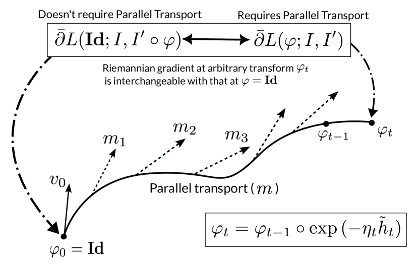
(a) Trick to avoid parallel transport in Riemannian Adaptive Optimization

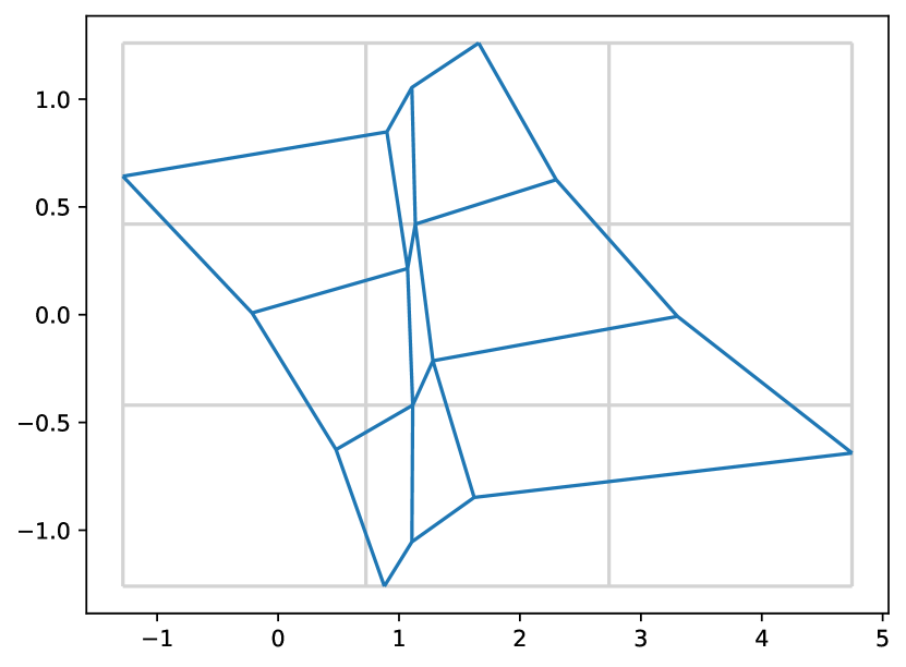
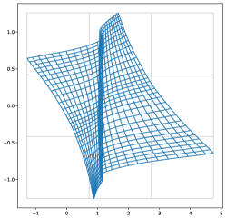
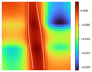
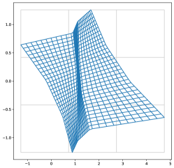
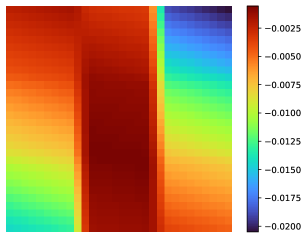
(b) Bicubic interpolation of diffeomorphic map does not preserve diffeomorphism

Figure S.3: Effect of downsampling on the warp and determinant of the Jacobian: We show the effect of downsampling on the warp and determinant of the Jacobian for a single image pair. The first column shows the initial warp, and the second and third columns show the warp and determinant of the Jacobian for the cubic and bilinear interpolations, respectively.

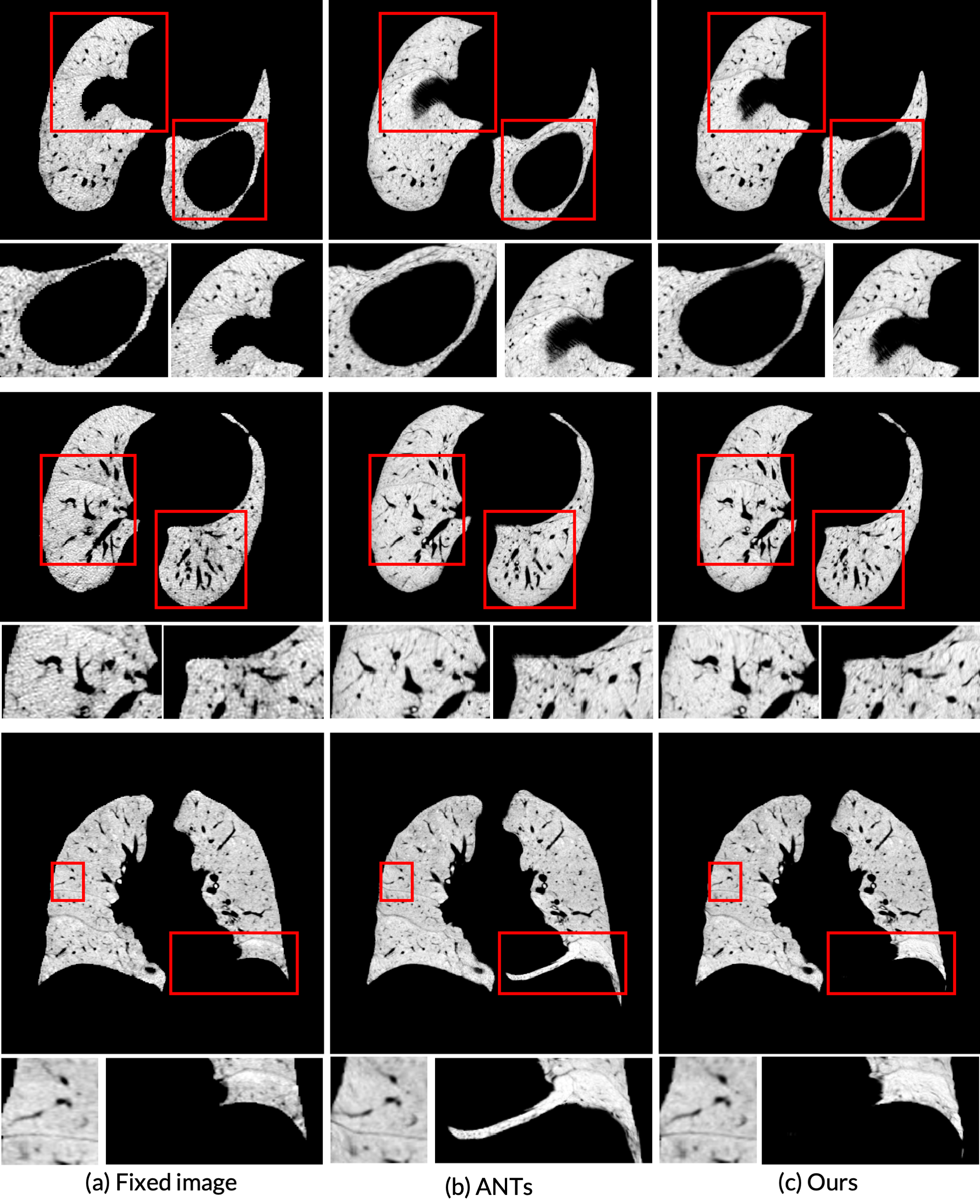
Figure S.4: Qualitative results on EMPIRE10 challenge: (a) shows the fixed image, (b) shows the registration performed by ANTs, and (c) our method, all with zoomed in regions. ANTs performs a coarse registration with ease, but still leaves out critical alignment of lung boundary and airways by not utilizing adaptive optimization. Our method performs perfectly diffeomorphic registration by construction, and does not lead to any registration errors, both in the lung boundaries or internal features.

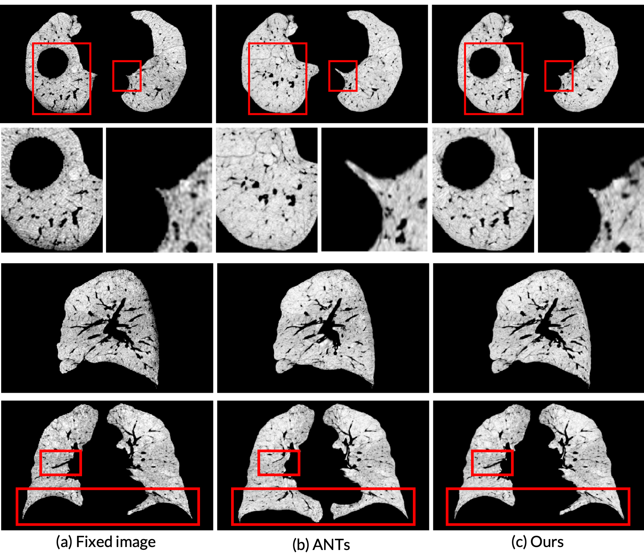
Figure S.5: More Qualitative results on EMPIRE10 challenge: (a) shows the fixed image, (b) shows the registration performed by ANTs, and (c) our method, all with zoomed in regions. ANTs performs a coarse registration with ease, but still leaves out critical alignment of lung boundary and airways by not utilizing adaptive optimization. Our method performs perfectly diffeomorphic registration by construction, and does not lead to any registration errors, both in the lung boundaries or internal features.

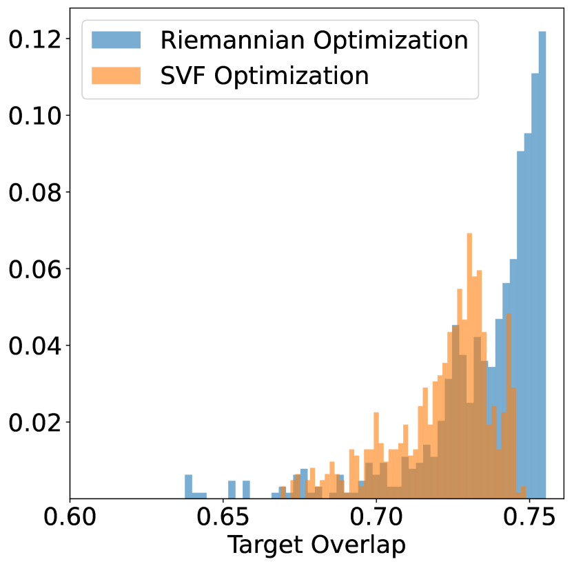
Figure S.6: Comparison of exponential versus direct optimization on LPBA40 dataset: We run the hyperparameter grid search on the LPBA40 dataset using direct Riemannian gradient updates with Adam optimizer (denoted as rgd), and optimizing the velocity field by computing the exponential map to represent the diffeomorphism (denoted as exp) across all the configurations shown in Fig. 6(a). The average target overlap for each configuration is then stored, and a histogram of target overlap values of the dataset is constructed. Note that the rgd variant has a significantly more number of configurations near the optimal value, and the average performance and the overall distribution of our optimization is better for the rgd variant than exp. Similar trends can be observed for the EMPIRE10 lung challenge in Fig. 3, where the exp representation underperforms for the same cost function, data, etc. Therefore, we recommend direct RGD optimization for diffeomorphisms.

References

- 1 G. Zhu, B. Jiang, L. Tong, Y. Xie, G. Zaharchuk, and M. Wintermark, “Applications of deep learning to neuro-imaging techniques,” Frontiers in neurology, vol. 10, p. 869, 2019.
- 2 E. M. Hillman, V. Voleti, W. Li, and H. Yu, “Light-sheet microscopy in neuroscience,” Annual review of neuroscience, vol. 42, pp. 295–313, 2019.
- 3 A. Routier, N. Burgos, M. Díaz, M. Bacci, S. Bottani, O. El-Rifai, S. Fontanella, P. Gori, J. Guillon, A. Guyot, et al., “Clinica: An open-source software platform for reproducible clinical neuroscience studies,” Frontiers in Neuroinformatics, vol. 15, p. 689675, 2021.
- 4 W.-L. Chen, J. Wagner, N. Heugel, J. Sugar, Y.-W. Lee, L. Conant, M. Malloy, J. Heffernan, B. Quirk, A. Zinos, et al., “Functional near-infrared spectroscopy and its clinical application in the field of neuroscience: advances and future directions,” Frontiers in neuroscience, vol. 14, p. 724, 2020.
- 5 A. Klein, J. Andersson, B. A. Ardekani, J. Ashburner, B. Avants, M.-C. Chiang, G. E. Christensen, D. L. Collins, J. Gee, P. Hellier, et al., “Evaluation of 14 nonlinear deformation algorithms applied to human brain mri registration,” Neuroimage, vol. 46, no. 3, pp. 786–802, 2009.
- 6 H. Qiu, C. Qin, A. Schuh, K. Hammernik, and D. Rueckert, “Learning diffeomorphic and modality-invariant registration using b-splines,” 2021.
- 7 W. Bai, H. Suzuki, J. Huang, C. Francis, S. Wang, G. Tarroni, F. Guitton, N. Aung, K. Fung, S. E. Petersen, et al., “A population-based phenome-wide association study of cardiac and aortic structure and function,” Nature medicine, vol. 26, no. 10, pp. 1654–1662, 2020.
- 8 J. Krebs, H. Delingette, B. Mailhé, N. Ayache, and T. Mansi, “Learning a probabilistic model for diffeomorphic registration,” IEEE transactions on medical imaging, vol. 38, no. 9, pp. 2165–2176, 2019.
- 9 Y. Fu, Y. Lei, T. Wang, K. Higgins, J. D. Bradley, W. J. Curran, T. Liu, and X. Yang, “Lungregnet: an unsupervised deformable image registration method for 4d-ct lung,” Medical physics, vol. 47, no. 4, pp. 1763–1774, 2020.
- 10 K. Murphy, B. Van Ginneken, J. M. Reinhardt, S. Kabus, K. Ding, X. Deng, K. Cao, K. Du, G. E. Christensen, V. Garcia, et al., “Evaluation of registration methods on thoracic ct: the empire10 challenge,” IEEE transactions on medical imaging, vol. 30, no. 11, pp. 1901–1920, 2011.
- 11 L. Nenoff, C. O. Ribeiro, M. Matter, L. Hafner, M. Josipovic, J. A. Langendijk, G. F. Persson, M. Walser, D. C. Weber, A. J. Lomax, et al., “Deformable image registration uncertainty for inter-fractional dose accumulation of lung cancer proton therapy,” Radiotherapy and Oncology, vol. 147, pp. 178–185, 2020.
- 12 I. Yoo, D. G. Hildebrand, W. F. Tobin, W.-C. A. Lee, and W.-K. Jeong, “ssemnet: Serial-section electron microscopy image registration using a spatial transformer network with learned features,” pp. 249–257, 2017.
- 13 A. Hand, T. Sun, D. Barber, D. Hose, and S. MacNeil, “Automated tracking of migrating cells in phase-contrast video microscopy sequences using image registration,” Journal of microscopy, vol. 234, no. 1, pp. 62–79, 2009.
- 14 M. Goubran, C. Leuze, B. Hsueh, M. Aswendt, L. Ye, Q. Tian, M. Y. Cheng, A. Crow, G. K. Steinberg, J. A. McNab, et al., “Multimodal image registration and connectivity analysis for integration of connectomic data from microscopy to mri,” Nature communications, vol. 10, no. 1, p. 5504, 2019.
- 15 Y. Rivenson, K. de Haan, W. D. Wallace, and A. Ozcan, “Emerging advances to transform histopathology using virtual staining,” BME frontiers, 2020.
- 16 J. Borovec, J. Kybic, I. Arganda-Carreras, D. V. Sorokin, G. Bueno, A. V. Khvostikov, S. Bakas, I. Eric, C. Chang, S. Heldmann, et al., “Anhir: automatic non-rigid histological image registration challenge,” IEEE transactions on medical imaging, vol. 39, no. 10, pp. 3042–3052, 2020.
- 17 G. Troglio, J. Le Moigne, J. A. Benediktsson, G. Moser, and S. B. Serpico, “Automatic extraction of ellipsoidal features for planetary image registration,” IEEE Geoscience and remote sensing letters, vol. 9, no. 1, pp. 95–99, 2011.
- 18 C. Chen, Y. Li, W. Liu, and J. Huang, “Sirf: Simultaneous satellite image registration and fusion in a unified framework,” IEEE Transactions on Image Processing, vol. 24, no. 11, pp. 4213–4224, 2015.
- 19 Y. Bentoutou, N. Taleb, K. Kpalma, and J. Ronsin, “An automatic image registration for applications in remote sensing,” IEEE transactions on geoscience and remote sensing, vol. 43, no. 9, pp. 2127–2137, 2005.
- 20 M. E. Linger and A. A. Goshtasby, “Aerial image registration for tracking,” IEEE Transactions on Geoscience and Remote Sensing, vol. 53, no. 4, pp. 2137–2145, 2014.
- 21 F. Pomerleau, F. Colas, R. Siegwart, et al., “A review of point cloud registration algorithms for mobile robotics,” Foundations and Trends® in Robotics, vol. 4, no. 1, pp. 1–104, 2015.
- 22 A. Collet, D. Berenson, S. S. Srinivasa, and D. Ferguson, “Object recognition and full pose registration from a single image for robotic manipulation,” pp. 48–55, 2009.
- 23 H. Balta, J. Velagic, H. Beglerovic, G. De Cubber, and B. Siciliano, “3d registration and integrated segmentation framework for heterogeneous unmanned robotic systems,” Remote Sensing, vol. 12, no. 10, p. 1608, 2020.
- 24 M. Beroiz, J. B. Cabral, and B. Sanchez, “Astroalign: A python module for astronomical image registration,” Astronomy and Computing, vol. 32, p. 100384, 2020.
- 25 Z. Li, Q. Peng, B. Bhanu, Q. Zhang, and H. He, “Super resolution for astronomical observations,” Astrophysics and Space Science, vol. 363, pp. 1–15, 2018.
- 26 D. Makovoz, T. Roby, I. Khan, and H. Booth, “Mopex: a software package for astronomical image processing and visualization,” vol. 6274, pp. 93–102, 2006.
- 27 D. Yang, H. Li, D. A. Low, J. O. Deasy, and I. El Naqa, “A fast inverse consistent deformable image registration method based on symmetric optical flow computation,” Physics in Medicine & Biology, vol. 53, no. 21, p. 6143, 2008.
- 28 M. Lefébure and L. D. Cohen, “Image registration, optical flow and local rigidity,” Journal of mathematical imaging and vision, vol. 14, pp. 131–147, 2001.
- 29 B. Glocker, N. Paragios, N. Komodakis, G. Tziritas, and N. Navab, “Optical flow estimation with uncertainties through dynamic mrfs,” in 2008 IEEE Conference on Computer Vision and Pattern Recognition, pp. 1–8, IEEE, 2008.
- 30 Q. Chen and V. Koltun, “Full flow: Optical flow estimation by global optimization over regular grids,” in Proceedings of the IEEE conference on computer vision and pattern recognition, pp. 4706–4714, 2016.
- 31 R. Bajcsy, R. Lieberson, and M. Reivich, “A computerized system for the elastic matching of deformed radiographic images to idealized atlas images.,” Journal of computer assisted tomography, vol. 7, no. 4, pp. 618–625, 1983.
- 32 J. C. Gee and R. K. Bajcsy, “Elastic matching: Continuum mechanical and probabilistic analysis,” Brain warping, vol. 2, pp. 183–197, 1998.
- 33 J. C. Gee, M. Reivich, and R. Bajcsy, “Elastically deforming a three-dimensional atlas to match anatomical brain images,” 1993.
- 34 G. E. Christensen and H. J. Johnson, “Consistent image registration,” IEEE transactions on medical imaging, vol. 20, no. 7, pp. 568–582, 2001.
- 35 G. E. Christensen, R. D. Rabbitt, and M. I. Miller, “Deformable templates using large deformation kinematics,” IEEE transactions on image processing, vol. 5, no. 10, pp. 1435–1447, 1996.
- 36 A. Trouvé, “Diffeomorphisms groups and pattern matching in image analysis,” International journal of computer vision, vol. 28, pp. 213–221, 1998.
- 37 G. E. Christensen, S. C. Joshi, and M. I. Miller, “Volumetric transformation of brain anatomy,” IEEE transactions on medical imaging, vol. 16, no. 6, pp. 864–877, 1997.
- 38 S. C. Joshi and M. I. Miller, “Landmark matching via large deformation diffeomorphisms,” IEEE transactions on image processing, vol. 9, no. 8, pp. 1357–1370, 2000.
- 39 E. D’agostino, F. Maes, D. Vandermeulen, and P. Suetens, “A viscous fluid model for multimodal non-rigid image registration using mutual information,” Medical image analysis, vol. 7, no. 4, pp. 565–575, 2003.
- 40 M. F. Beg, M. I. Miller, A. Trouvé, and L. Younes, “Computing large deformation metric mappings via geodesic flows of diffeomorphisms,” International journal of computer vision, vol. 61, pp. 139–157, 2005.
- 41 M. Niethammer, Y. Huang, and F.-X. Vialard, “Geodesic regression for image time-series,” pp. 655–662, 2011.
- 42 M. Niethammer, R. Kwitt, and F.-X. Vialard, “Metric learning for image registration,” June 2019.
- 43 R. Kwitt and M. Niethammer, “Fast predictive simple geodesic regression,” p. 267, 2017.
- 44 B. Avants and J. C. Gee, “Geodesic estimation for large deformation anatomical shape averaging and interpolation,” Neuroimage, vol. 23, pp. S139–S150, 2004.
- 45 B. B. Avants, C. L. Epstein, M. Grossman, and J. C. Gee, “Symmetric diffeomorphic image registration with cross-correlation: evaluating automated labeling of elderly and neurodegenerative brain,” Medical image analysis, vol. 12, no. 1, pp. 26–41, 2008.
- 46 G. Balakrishnan, A. Zhao, M. R. Sabuncu, J. Guttag, and A. V. Dalca, “Voxelmorph: a learning framework for deformable medical image registration,” IEEE transactions on medical imaging, vol. 38, no. 8, pp. 1788–1800, 2019.
- 47 T. C. Mok and A. C. Chung, “Large deformation diffeomorphic image registration with laplacian pyramid networks,” pp. 211–221, 2020.
- 48 J. Chen, E. C. Frey, Y. He, W. P. Segars, Y. Li, and Y. Du, “Transmorph: Transformer for unsupervised medical image registration,” Medical image analysis, vol. 82, p. 102615, 2022.
- 49 S. Zhao, Y. Dong, E. I. Chang, Y. Xu, et al., “Recursive cascaded networks for unsupervised medical image registration,” pp. 10600–10610, 2019.
- 50 T. C. Mok and A. C. Chung, “Conditional deformable image registration with convolutional neural network,” pp. 35–45, 2021.
- 51 M. Hoffmann, B. Billot, D. N. Greve, J. E. Iglesias, B. Fischl, and A. V. Dalca, “Synthmorph: learning contrast-invariant registration without acquired images,” IEEE transactions on medical imaging, vol. 41, no. 3, pp. 543–558, 2021.
- 52 X. Jia, J. Bartlett, T. Zhang, W. Lu, Z. Qiu, and J. Duan, “U-net vs transformer: Is u-net outdated in medical image registration?,” arXiv preprint arXiv:2208.04939, 2022.
- 53 J. Ashburner, “A fast diffeomorphic image registration algorithm,” Neuroimage, vol. 38, no. 1, pp. 95–113, 2007.
- 54 T. Tieleman, G. Hinton, et al., “Lecture 6.5-rmsprop: Divide the gradient by a running average of its recent magnitude,” COURSERA: Neural networks for machine learning, vol. 4, no. 2, pp. 26–31, 2012.
- 55 D. P. Kingma and J. Ba, “Adam: A method for stochastic optimization,” arXiv preprint arXiv:1412.6980, 2014.
- 56 J. Duchi, E. Hazan, and Y. Singer, “Adaptive subgradient methods for online learning and stochastic optimization.,” Journal of machine learning research, vol. 12, no. 7, 2011.
- 57 S. Bonnabel, “Stochastic gradient descent on riemannian manifolds,” IEEE Transactions on Automatic Control, vol. 58, no. 9, pp. 2217–2229, 2013.
- 58 M. Kochurov, R. Karimov, and S. Kozlukov, “Geoopt: Riemannian optimization in pytorch,” 2020.
- 59 N. Boumal, B. Mishra, P.-A. Absil, and R. Sepulchre, “Manopt, a Matlab toolbox for optimization on manifolds,” Journal of Machine Learning Research, vol. 15, no. 42, pp. 1455–1459, 2014.
- 60 B. B. Avants, N. Tustison, G. Song, et al., “Advanced normalization tools (ants),” Insight j, vol. 2, no. 365, pp. 1–35, 2009.
- 61 T. Vercauteren, X. Pennec, A. Perchant, N. Ayache, et al., “Diffeomorphic demons using itk’s finite difference solver hierarchy,” The Insight Journal, vol. 1, 2007.
- 62 G. M. Fleishman, “Bigstream.” https://github.com/GFleishman/bigstream, 2023. GitHub repository.
- 63 A. Hering, L. Hansen, T. C. Mok, A. C. Chung, H. Siebert, S. Häger, A. Lange, S. Kuckertz, S. Heldmann, W. Shao, et al., “Learn2reg: comprehensive multi-task medical image registration challenge, dataset and evaluation in the era of deep learning,” IEEE Transactions on Medical Imaging, vol. 42, no. 3, pp. 697–712, 2022.
- 64 “Rnr-exm grand challenge.”
- 65 L. R. Dice, “Measures of the amount of ecologic association between species,” Ecology, vol. 26, no. 3, pp. 297–302, 1945.
- 66 F. Chen, P. W. Tillberg, and E. S. Boyden, “Expansion microscopy,” Science, vol. 347, no. 6221, pp. 543–548, 2015.
- 67 A. T. Wassie, Y. Zhao, and E. S. Boyden, “Expansion microscopy: principles and uses in biological research,” Nature methods, vol. 16, no. 1, pp. 33–41, 2019.
- 68 D. Gambarotto, F. U. Zwettler, M. Le Guennec, M. Schmidt-Cernohorska, D. Fortun, S. Borgers, J. Heine, J.-G. Schloetel, M. Reuss, M. Unser, et al., “Imaging cellular ultrastructures using expansion microscopy (u-exm),” Nature methods, vol. 16, no. 1, pp. 71–74, 2019.
- 69 F. Chen, A. T. Wassie, A. J. Cote, A. Sinha, S. Alon, S. Asano, E. R. Daugharthy, J.-B. Chang, A. Marblestone, G. M. Church, et al., “Nanoscale imaging of rna with expansion microscopy,” Nature methods, vol. 13, no. 8, pp. 679–684, 2016.
- 70 U. Grenander and M. I. Miller, “Computational anatomy: An emerging discipline,” Quarterly of applied mathematics, vol. 56, no. 4, pp. 617–694, 1998.
- 71 A. W. Toga and P. M. Thompson, “The role of image registration in brain mapping,” Image and vision computing, vol. 19, no. 1-2, pp. 3–24, 2001.
- 72 A. Gholipour, N. Kehtarnavaz, R. Briggs, M. Devous, and K. Gopinath, “Brain functional localization: a survey of image registration techniques,” IEEE transactions on medical imaging, vol. 26, no. 4, pp. 427–451, 2007.
- 73 D. S. Marcus, T. H. Wang, J. Parker, J. G. Csernansky, J. C. Morris, and R. L. Buckner, “Open access series of imaging studies (oasis): cross-sectional mri data in young, middle aged, nondemented, and demented older adults,” Journal of cognitive neuroscience, vol. 19, no. 9, pp. 1498–1507, 2007.
- 74 Q. Wang, S.-L. Ding, Y. Li, J. Royall, D. Feng, P. Lesnar, N. Graddis, M. Naeemi, B. Facer, A. Ho, et al., “The allen mouse brain common coordinate framework: a 3d reference atlas,” Cell, vol. 181, no. 4, pp. 936–953, 2020.
- 75 T. Sentker, F. Madesta, and R. Werner, “Gdl-fire: Deep learning-based fast 4d ct image registration,” in International Conference on Medical Image Computing and Computer-Assisted Intervention, pp. 765–773, Springer, 2018.
- 76 E. Haber and J. Modersitzki, “Numerical methods for volume preserving image registration,” Inverse problems, vol. 20, no. 5, p. 1621, 2004.
- 77 A. Banyaga, The structure of classical diffeomorphism groups, vol. 400. Springer Science & Business Media, 2013.
- 78 J. Leslie, “On a differential structure for the group of diffeomorphisms,” Topology, vol. 6, no. 2, pp. 263–271, 1967.
- 79 L. Younes, Shapes and diffeomorphisms, vol. 171. Springer, 2010.
- 80 C. Chevalley, “Théorie des groupes de lie,” (No Title), 1951.
- 81 B. Mertzios and M. Christodoulou, “On the generalized cayley-hamilton theorem,” IEEE transactions on automatic control, vol. 31, no. 2, pp. 156–157, 1986.
- 82 C. Moler and C. Van Loan, “Nineteen dubious ways to compute the exponential of a matrix, twenty-five years later,” SIAM review, vol. 45, no. 1, pp. 3–49, 2003.
- 83 B. C. Hall and B. C. Hall, Lie groups, Lie algebras, and representations. Springer, 2013.
- 84 B. C. Hall, “An elementary introduction to groups and representations,” arXiv preprint math-ph/0005032, 2000.
- 85 H. Zhang, S. J Reddi, and S. Sra, “Riemannian svrg: Fast stochastic optimization on riemannian manifolds,” Advances in Neural Information Processing Systems, vol. 29, 2016.
- 86 G. Bécigneul and O.-E. Ganea, “Riemannian adaptive optimization methods,” arXiv preprint arXiv:1810.00760, 2018.
- 87 ANTsX, “Antsx: Advanced normalization tools (ants).” GitHub repository.
- 88 A. C. Evans, D. L. Collins, S. Mills, E. D. Brown, R. L. Kelly, and T. M. Peters, “3d statistical neuroanatomical models from 305 mri volumes,” pp. 1813–1817, 1993.