Open-Vocabulary Federated Learning with Multimodal Prototyping

Abstract

Existing federated learning (FL) studies usually assume the training label space and test label space are identical. However, in real-world applications, this assumption is too ideal to be true. A new user could come up with queries that involve data from unseen classes, and such open-vocabulary queries would directly defect such FL systems. Therefore, in this work, we explicitly focus on the under-explored open-vocabulary challenge in FL. That is, for a new user, the global server shall understand her/his query that involves arbitrary unknown classes. To address this problem, we leverage the pre-trained vision-language models (VLMs). In particular, we present a novel adaptation framework tailored for VLMs in the context of FL, named as Federated Multimodal Prototyping (Fed-MP). Fed-MP adaptively aggregates the local model weights based on light-weight client residuals, and makes predictions based on a novel multimodal prototyping mechanism. Fed-MP exploits the knowledge learned from the seen classes, and robustifies the adapted VLM to unseen categories. Our empirical evaluation on various datasets validates the effectiveness of Fed-MP.

capbtabboxtable[][]

Open-Vocabulary Federated Learning with Multimodal Prototyping

Huimin Zeng  Zhenrui Yue  Dong Wang Unversity of Illinois at Urbana-Champaign {huiminz3, zhenrui3, dwang24}@illinois.edu

1 Introduction

Federated learning (FL) emerges as a new machine learning (ML) paradigm that trains ML models from decentralized data sources McMahan et al. (2017). The decentralized nature of FL makes it a promising solution for privacy-sensitive applications across numerous domains (e.g., natural language processing Liu et al. (2021), multimodal learning Che et al. (2023), visual recognition Liu et al. (2020)). In FL, there exists a central server storing a global model, and a set of clients. The clients will collaboratively train the global model without sharing their private data. While numerous FL studies have been proposed, the elusive open-vocabulary challenge is largely under-explored.

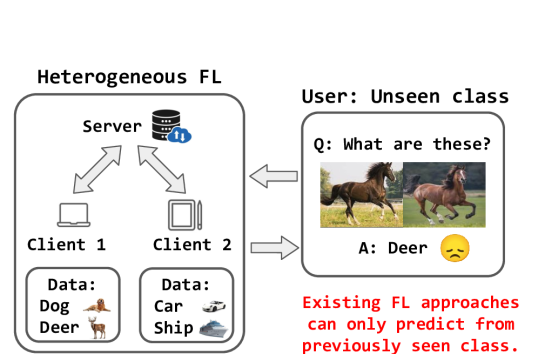
Figure 1: A non open-vocabulary FL model could only return a prediction from the seen classes for an open-vocabulary query.

Traditional FL studies (e.g., domain-generalized federated learning) usually assume that the label space of training data and test data is identical. Based on this assumption, the proposed FL methods are not open-vocabulary by design. However, in real-world applications, new users might send queries that involve novel classes, e.g., identifying an object in a photo. If the category of this object is never seen in the training data, then traditional FL systems simply fail and can only predict from previously seen classes as shown in Figure 1.

Indeed, in centralized ML, there exist methods to predict unseen classes Shu et al. (2018); He et al. (2022); Changpinyo et al. (2017). However, they usually require a huge amount of the training data and could not tackle new addition of unseen classes over time Kuchibhotla et al. (2022). More importantly, the unique challenge of data heterogeneity in FL makes centralized methods inapplicable to train FL models Jiang et al. (2022); Xu et al. (2022); Zhang et al. (2023). The data heterogeneity in FL is the heterogeneity in client data distributions. For instance, in Figure 1, there are only images of dog and deer in client 1, and client 2 only has images of car and ship. Such non-i.i.d. data across clients is heterogeneous data. Therefore, in this work, we explicitly focus on the open-vocabulary challenge in FL: how can we build an FL framework that is open-vocabulary?

On the other hand, exploiting the pre-trained vision-language models (VLMs) (e.g., CLIP) for FL has recently gained increased attention for their strong generalization ability Lu et al. (2023). With CLIP, the community could address data heterogeneity, personalization and generalization in FL Lu et al. (2023); Yang et al. (2023); Guo et al. (2023a). Technically, to adapt CLIP for specific FL applications, existing methods mainly adopt prompt learning. Prompt learning optimizes a set of learnable soft prompt vectors, and prepends them to input embeddings Lu et al. (2023); Yang et al. (2023); Guo et al. (2023a). As such, domain-specific knowledge is integrated into the features extracted by CLIP, leading to improved performance on downstream tasks. Unfortunately, these learned prompts usually suffer from generalizing well to novel unseen classes during test, and yet, no proper solution has been developed.

Therefore, in this work, we focus on addressing the elusive open-vocabulary challenge in FL. To the best of our knowledge, we are the first to propose a CLIP-based FL framework that is explicitly tailored for the open-vocabulary setting. To achieve open-vocabulary FL, we propose a federated finetuning framework tailored for VLMs: Federated Multimodal Prototyping or Fed-MP. Intuitively, Fed-MP has two design objectives: 1) low communication overhead between the server and clients in FL: given the large size of CLIP, Fed-MP must be light-weight and affordable in terms of model training in an FL application; 2) open-vocabulary: the global model shall understand the queries that involve arbitrary unseen classes.

To this end, Fed-MP consists of two modules. Firstly, Fed-MP adaptively aggregates the local model weights based on the similarity between new queries and perturbed client prompt representations. These prompt representations are perturbed by a set of learnable parameters, which is defined as client residuals. Client residuals protect clients’ class information by perturbing the text representations. In addition, with client residuals, locally learned visual concepts are integrated into the perturbed prompt representations as well. This similarity-based design is realistic and practical in terms of real-world applications: a user comes to use the FL system, and she/he sends a set of queries to the server. In return, the server should adaptively obtain an aggregated model that is aligned with the interest of the user. Secondly, we design a multimodal prototyping mechanism to make predictions for the open-vocabulary queries. The multimodal prototypes include text prototypes and visual prototypes. The text prototypes are the original encoded text prompts in the new queries. As for the visual prototypes, they are normalized visual features extracted by CLIP image encoder with pseudo labeling. During inference, Fed-MP predicts for a query image based on its weighted distance to text prototypes and visual prototypes. Both modules are designed to exploit the knowledge learned from the seen classes during training. Under Fed-MP, the adapted CLIP model generalizes well to test images from unseen classes, achieving open-vocabulary federated learning.

We summarize the contributions of our paper as follows:

1. To the best of our knowledge, Fed-MP is the first VLM-based FL framework that explicitly addresses the open-vocabulary challenge in FL applications.

2. Technically, to build Fed-MP, we present a novel adaptive aggregation protocol and a novel multimodal prototyping mechanism.

3. Extensive experimental results on 6 image classification datasets suggest that Fed-MP can effectively improve model performance on test data from unseen categories, outperforming the state-of-the-art baselines.

2 Related Work

2.1 Federated Learning with Domain Generalization

Domain generalization (DG) in FL aims to improve model’s generalization on the unknown test clients or the unknown global data with domain shifts. Due to privacy concerns (no data exchange) and data heterogeneity, existing centralized DG methods become inapplicable and infeasible in FL Jiang et al. (2022); Zhang et al. (2023); Xu et al. (2022); Sun et al. (2023). Therefore, a few studies start to investigate DG in FL. For instance, Jiang et al. (2022) propose to establish a harmonized feature space on the frequency domain and aggregate local models with flat optima, so that both local shift and global shift could be rectified. In comparison, for generalization, Zhang et al. (2023) introduce a variance reduction regularizer to encourage fairness of the generalization gap among the clients. Finally, in (Sun et al., 2023), feature distribution matching is proposed to learn domain-invariant client features, so that the model generalizes to unseen clients. However, the above methods all assume that the label space of training data and test data is identical: all tested categories have to be seen during training despite domain shifts. In other words, these methods are not open-vocabulary, and could not handle queries with unseen classes.

2.2 Federated Learning with Vision-Language Models

Recently, integrating vision-language models (e.g., CLIP) into FL has gained increased attention for their strong generalization ability. For instance, Guo et al. (2023a, b) focus on learning soft textual prompts to personalize CLIP on client data by extending Zhou et al. (2022) into the federated setting, whereas Li et al. (2023) leverage visual prompts to achieve the same goal. In addition to prompt learning, Lu et al. (2023); Chen et al. (2023); Qiu et al. (2023) fine-tune CLIP with light-weight neural networks (i.e., adapters) to adapt CLIP to FL applications. However, the above methods are not deliberately designed for open-vocabulary settings. Even though the method presented in Qiu et al. (2023) was tested with open-vocabulary queries, its performance purely counts on the unreliable generalization of the learned adapter. In comparison, in this work, we explicitly focus on addressing the open-vocabulary challenge in FL, and present the first FL framework that is tailored for open-vocabulary queries.

3 Preliminaries

3.1 Federated Learning

Assume there are $K$ clients in an FL application. For all clients, each data point is characterized by an input feature ${x}\sim\mathcal{X}$ and a label $y\sim\mathcal{Y}$. On client $k$, its local dataset $\mathcal{D}^{(k)}$ is denoted as $\mathcal{D}^{(k)}=\{({x}_{1}^{(k)},y_{1}^{(k)}),...|({x}_{i}^{(k)},y_{i}^{(k)})\sim p^{(k)}\}$, where $p^{(k)}$ represents the local data distribution on client $k$. For simplicity, if not specified, we use the notations without the client index $k$ to represent an arbitrary client.

To find the optimal global model $f_{\theta}^{*}$ in an FL application, McMahan et al. (2017) propose Federated Averaging (FedAvg). Under FedAvg, at each round, each local client firstly receives a copy of the global model $f_{\theta}$ from the central server and trains the model with its own data. This leads to different local models $(f^{(1)}_{\theta},f^{(2)}_{\theta},...,f^{(K)}_{\theta})$. Then, clients send the trained model weights to the central server. Finally, on the central server, the global model will be updated using a weighted-average of the received model weights based on the size of each local dataset.

Note that, the local data distributions on different clients could be non-i.i.d. and have exclusive label spaces. More importantly, in a real-world application, a new user of the FL system might send queries that involve objects from unseen categories. For instance, in Figure 1, the training classes are dog, deer, car, and ship, whereas the test query is an image of horse.

3.2 CLIP: Contrastive Language-Image Pre-training

CLIP is a language-grounded image classifier. It predicts which images are paired with which texts. Formally, we use $f_{I}$ to denote the CLIP image encoder, and $f_{T}$ for the CLIP text encoder. The inference process and training process of CLIP are:

• Inference: For a query image $x$ and $|\mathcal{Y}|$ classes, we firstly craft a set of candidate prompts that contain class information (e.g., {a photo of [class 1], a photo of [class 2]...}). Then, CLIP encodes $x$ into a visual representation $z$, and encodes the candidate prompts into text representations $\{t_{{candidate}_{1}},t_{{candidate}_{2}},...,t_{{candidate}_{{|\mathcal{Y}|}}}\}$. After computing cosine similarity between the $z$ and candidate prompt representations, CLIP selects the prompt with the highest cosine similarity as the final prediction:

  $$\begin{split}&\hat{y}=\arg\max_{c}\frac{\mathrm{exp}\big{(}\mathrm{cos}(z,t_{{candidate}_{c}})/\tau\big{)}}{\sum_{c^{\prime}}\mathrm{exp}\big{(}\mathrm{cos}(z,t_{candidate_{c^{\prime}}})/\tau\big{)}},\\ &\text{where}\;z=f_{I}(x),\\ &t_{{candidate}_{c}}=f_{T}(\texttt{a photo of [class c]}),\\ &c\in\{1,2,...,|\mathcal{Y}|\}.\end{split}$$ (1)

• Training: For a training set $\mathcal{D}$, we construct a ground truth prompt $t_{gt_{i}}$ for each image $x_{i}$. For $x_{i}$, its ground truth prompt contains textual description of its class label $y_{i}$. Then, the CLIP contrastive loss Radford et al. (2021) is computed over all visual representations $z_{i}$s and text representations $t_{{gt}_{i}}$s:

  $$\begin{split}\mathcal{L}_{CLIP}&=\frac{1}{|\mathcal{D}|}\sum_{i=1}^{|\mathcal{D}|}-\log\frac{e^{{z}_{i}\cdot t_{gt_{i}}}}{\sum_{j=1}^{|\mathcal{D}|}e^{{z}_{i}\cdot t_{gt_{j}}}}\\ &+\frac{1}{|\mathcal{D}|}\sum_{i=1}^{|\mathcal{D}|}-\log\frac{e^{{z}_{i}\cdot t_{gt_{i}}}}{\sum_{j=1}^{|\mathcal{D}|}e^{{z}_{j}\cdot t_{gt_{i}}}}.\end{split}$$ (2)

4 Algorithm

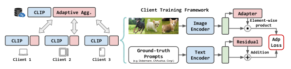
Figure 2: The training and aggregation process of Fed-MP. On clients, the adapters and residuals are trained using local data. In adaptive aggregation, only the adapter weights are aggregated.

4.1 Parameter-Efficient Adaptation

Given existing parameter-efficient finetuning (PEFT) methods, any of them could be used by Fed-MP to adapt the CLIP model in FL. In our implementation, we choose to add a small two-layer fully connected network for the visual modality as in Lu et al. (2023). Formally, we define the adapter as $f_{A}$. As shown in Figure 2, for an input image $x$, $f_{A}$ takes its visual representation as input, i.e., $f_{A}(z),z=f_{I}(x)$. $f_{A}$ returns a vector of normalized importance scores with the same dimensionality of $z$. Finally, the adapted visual representation $z^{\prime}$ is computed by multiplying $f_{A}(z)$ with $z$ element-wisely:

$$z^{\prime}=f_{A}(z)\odot z,\;\;\mathrm{where}\;z=f_{I}(x).$$ (3)

Note that during training, the weights of visual adapter are sent to the global server for aggregation instead of the entire CLIP model.

4.2 Client Residuals

In an open-vocabulary setting, a new user will send test queries that involve unseen data categories. Thus, to fully exploit the learned knowledge from client data, it is critical to consider the semantic closeness between the clients and the new user when performing model aggregation. Intuitively, the importance weights of local clients should be increased if they are semantically closer to the new user. For instance, client 1 only contains images and prompts of ’Doberman’, and client 2 only has images and prompts of ’Tabby cat’. Assume a test query contains an image of a dog, and the candidates prompts are ’a photo of German shepherd’ and ’a photo of Welsh Corgi’. In this example, the test class names ’German shepherd’ and ’Welsh Corgi’ are unseen during training. However, it is intuitive that client 1 is semantically closer to the test query than client 2. The reason is that the prompts of client 1 and the test prompts are all related to dog. Therefore, when aggregating the global model, the importance weight of client 1 should be higher than client 2.

However, existing studies mainly use FedAvg without considering such semantic closeness, and therefore, are not adaptive to open-vocabulary queries. Moreover, directly comparing client class names and the test classes causes privacy leakage: it requires the clients to share class information with the server. Therefore, inspired by Yu et al. (2023), we proposed to add a set of learnable perturbations to perturb the encoded text prompts for all clients. Such design protects class information on clients. More importantly, these perturbations will interact with images during training. As such, they provide aligned semantic information from both texts and images.

Formally, we define such perturbations as client residuals. The client residuals on a specific client are a set of learnable perturbations $\Delta=\{\delta_{1},\delta_{2},...,\delta_{|\mathcal{Y}|}\}$. Each $\delta_{c}\in\Delta$ corresponds to a specific class $c$, and has the same dimensionality of a prompt representation. When computing the prompt presentations with residuals, CLIP will element-wisely add them to the prompt representations of corresponding classes. For instance, for the ground truth prompt of sample $(x_{i},y_{i})$, its prompt representation with residual is computed as

$$\begin{split}&t^{{}^{\prime}}_{{gt}_{i}}=t_{{gt}_{i}}+\alpha\delta_{y_{i}},\end{split}$$ (4)

where $\delta_{y_{i}}$ is the perturbation for class $y_{i}$ (Figure 2), and $\alpha$ is a non-negative scaling factor.

With both trainable adapter and client residuals, the adaptation loss of CLIP on the training set $\mathcal{D}=\{(x_{i},y_{i})\}$ is computed as follows:

$$\begin{split}\mathcal{L}_{adp}(f_{A},\delta)&=\frac{1}{|\mathcal{D}|}\sum_{i=1}^{|\mathcal{D}|}-\log\frac{e^{{z}^{{}^{\prime}}_{i}\cdot t^{{}^{\prime}}_{gt_{i}}}}{\sum_{j=1}^{|\mathcal{D}|}e^{{z}^{{}^{\prime}}_{i}\cdot t^{{}^{\prime}}_{gt_{j}}}}\\ &+\frac{1}{|\mathcal{D}|}\sum_{i=1}^{|\mathcal{D}|}-\log\frac{e^{{z}^{{}^{\prime}}_{i}\cdot t^{{}^{\prime}}_{gt_{i}}}}{\sum_{j=1}^{|\mathcal{D}|}e^{{z}^{{}^{\prime}}_{j}\cdot t^{{}^{\prime}}_{gt_{i}}}}.\end{split}$$ (5)

In Equation  5, $z^{{}^{\prime}}$ represents the adapted visual representation. $t^{{}^{\prime}}_{gt}$ is the perturbed text presentation.

After training, the client residuals are added to the encoded candidate prompts, according to the class names. This process returns a set of perturbed representations of candidate prompts:

$$\mathcal{T}^{\prime}=\{t^{{}^{\prime}}_{{candidate}_{1}},t^{{}^{\prime}}_{{candidate}_{2}},...,t^{{}^{\prime}}_{{candidate}_{|\mathcal{Y}|}}\},$$ (6)

where $t^{{}^{\prime}}_{{candidate}_{c}}=t_{{candidate}_{c}}+\delta_{c}$. The client will send $\mathcal{T}^{\prime}$ to the central server along with the updated adapter. This process will not lead to privacy leakage, as the class names and the training data are not shared with the server.

4.3 Adaptive Model Aggregation with Client Residuals

After receiving $f^{(1)}_{A}$, $f^{(2)}_{A}$, …, $f^{(K)}_{A}$ and $\mathcal{T}^{\prime(1)}$, $\mathcal{T}^{\prime(2)}$, …, $\mathcal{T}^{\prime(K)}$, the central server will then aggregate the adapter weights based on the queries from the new user. The aggregation protocol is based on the similarity between the queries of the new user and the perturbed prompt representations of different clients, namely $\mathcal{T}^{\prime(1)}$, $\mathcal{T}^{\prime(2)}$, …, $\mathcal{T}^{\prime(K)}$.

In particular, assume the new user has a set of unlabeled test images $\mathcal{D}_{test}$ and a set of candidate prompts. Note that the test label space $\mathcal{Y}_{test}$ and the client label space $\mathcal{Y}^{(k)}$ is mutually exclusive: $\mathcal{Y}_{test}\cap\mathcal{Y}^{(k)}=\varnothing,k=1,...,K$.

The first step of adaptive aggregation is to encode the test candidate prompts using the CLIP text encoder. This returns a set of prompt representations that correspond the test classes:

$$\begin{split}&\mathcal{T}_{test}=\{t_{{test}_{1}},t_{{test}_{2}},...,t_{{test}_{|\mathcal{Y}_{test}|}}\},\\ &\mathrm{where}\;\;t_{test_{c}}=f_{T}(\texttt{a photo of [test class c]}).\end{split}$$ (7)

For instance, in Figure 1, test prompts could be "a photo of [horse]" and "a photo of [cat]", where both [horse] and [cat] are classes never seen during training.

Next, the server measures the semantic closeness between the new user and all clients. Specifically, it computes the expected similarity between $\mathcal{T}_{test}$ and $\mathcal{T}^{\prime(1)}$, $\mathcal{T}^{\prime(2)}$, …, $\mathcal{T}^{\prime(K)}$, respectively. For instance, we define the expected similarity between the new user and client $k$ as $\xi_{k}$. It is computed via:

$$\begin{split}&\xi_{k}=\mathbb{E}_{t_{test}\sim\mathcal{T}_{test},t^{{}^{\prime}}_{candidate}\sim\mathcal{T}^{{}^{\prime}(k)}}\big{[}\mathrm{cos}(t_{test},t^{\prime}_{candidate})\big{]}\\ &=\frac{1}{|\mathcal{Y}_{test}||\mathcal{Y}^{(k)}|}\sum_{l=1}^{|\mathcal{Y}_{test}|}\sum_{m=1}^{|\mathcal{Y}^{(k)}|}\mathrm{cos}(t_{test_{l}},t^{{}^{\prime}(k)}_{candidcate_{m}}).\end{split}$$ (8)

Note that Equation 8 computes the averaged cosine similarity between any two encoded prompts, one from the new user and one from client $k$. Moreover, Equation 8 does not cause privacy leakage as elaborated in Section 4.2.

After computing the expected similarity for all clients, the server aggregates the adapter weights:

$$\begin{split}&\theta^{*}_{A}=\frac{1}{\sum_{k}e^{\xi_{k}}}\sum_{k=1}^{K}e^{\xi_{k}}\cdot{\theta}^{(k)}_{A}.\end{split}$$ (9)

In Equation 9, $\theta^{*}_{A}$ is the aggregated adapter weights. $\theta^{(k)}_{A}$ represents the adapter weights uploaded by client $k$. Compared to FedAvg, Equation 9 takes the semantic closeness of the new user and the clients into account. The rationale behind this design is that semantically closer clients have learned more useful visual concepts related to the open-vocabulary queries, whereas other clients may only learned irrelevant concepts. As such, useful visual concepts should be highlighted and integrated to the adapted CLIP by up-weighting corresponding adpater weights.

4.4 Multimodal Prototyping

Recall that during inference, for a query image, CLIP will compare the cosine similarity between its visual representation and the representations of candidate prompts (Equation 1). In this context, these prompt representations are by default text prototypes for the test classes. This is because the predictions are produced by measuring the distance (cosine similarity) between the text prototypes and the representation of the input image. Thus, the representations of candidate prompts are defined as the textual prototypes $\{p_{1},p_{2},...,p_{|\mathcal{Y}_{test}|}\}$:

$$\{p_{1},p_{2},...,p_{|\mathcal{Y}_{test}|}\},\;\mathrm{where}\;p_{i}=t_{test_{i}}.$$ (10)

However, the global model has never seen textual prototypes of unseen classes. This leads to poor generalization.

Therefore, based on the aggregated global model, we further propose to develop a new set of visual prototypes. In particular, inspired by Iwasawa and Matsuo (2021), for each test class, we define a visual prototype set. Formally, for test class $c$, its visual prototype set is defined as $\mathcal{Q}_{c}$.

If the new user send an extensive amount of queries, the global server may need to process them in mini-batches. In this case, we introduce a time stamp $n$ to denote the temporal order of the test process. Meanwhile, the update process follows the same temporal order. At $n=0$, $Q$s are initialized as empty sets. Then, for a test sample $x$ at time step $n$, the visual prototypes are updated as follows:

$$\mathcal{Q}^{n+1}_{\hat{y}}=\begin{cases}\mathcal{Q}^{n}_{\hat{y}}\cap\{\frac{z^{\prime}}{||z^{\prime}||}\},&\text{if }\mathcal{H}(x)\leq\epsilon\\ \mathcal{Q}^{n}_{\hat{y}},&\text{otherwise}\end{cases}$$ (11)

where $z^{\prime}$ is the adapted representation of $x$. $\hat{y}$ is the pseudo prediction calculated by the adapted CLIP: $\hat{y}=\arg\max_{c}\frac{\mathrm{exp}\big{(}\mathrm{cos}(z^{\prime},t_{{test}_{c}})/\tau\big{)}}{\sum_{c^{\prime}}\mathrm{exp}\big{(}\mathrm{cos}(z^{\prime},t_{test{c^{\prime}}})/\tau\big{)}}$. $\mathcal{H}(x)$ is the entropy of the predictive probabilities, evaluating the quality of the prediction: $\mathcal{H}(x)=\sum_{c=1}^{|\mathcal{Y}_{test}|}-P(\hat{y}=c|x)\mathrm{log}P(\hat{y}=c|x)$ as in Iwasawa and Matsuo (2021). $\epsilon$ is confidence threshold.

According to Equation 11, only one prototype set (class $\hat{y}$) would be updated based on the pseudo prediction. Moreover, in our implementation, we implemented Equation 11 in an efficient way, so that there is no need to save all the visual representations (Appendix A).

Eventually, with the visual prototypes, Fed-MP computes the prediction for the next $x$ based on its distance towards the centroids of the multimodal prototypes. Specifically, under multimodal prototyping, CLIP makes the prediction for $x$ by selecting the closest multimodal prototypes:

$$\begin{split}&\hat{y}=\arg\max_{c}\big{[}\mathrm{cos}(z^{\prime},p_{c})+\mathrm{cos}(z^{\prime},\bar{q}_{c})\big{]},\end{split}$$ (12)

where $p_{c}$ is the textual prototype of [test class c] and $\bar{q}_{c}$ is the centroid of visual prototypes of [test class c]:

$$\bar{q}_{c}=\frac{1}{|Q_{c}|}\sum_{q\in Q_{c}}q.$$ (13)

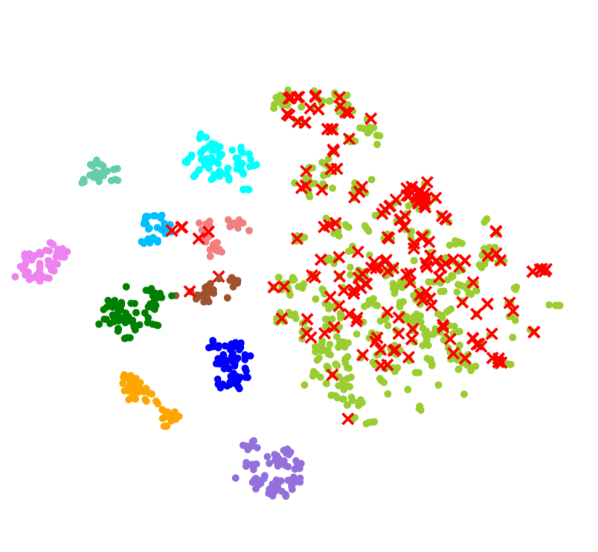
(a) w/o Prototyping

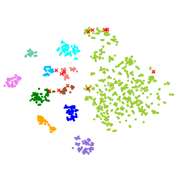
(b) with Prototyping

Figure 3: T-SNE visualization on test classes from Caltech101.

The rationale behind multimodal prototyping is: if a test sample obtains a high-quality prediction, then it could serve as a template for other test samples. Moreover, under Fed-MP, the adapted visual representations are semantic-aware, because the global model aggregation is based on the semantic closeness between the clients (training classes) and new user (test classes). Therefore, in addition to textual prototypes, the visual prototypes could also contribute to the model generalization on test data from unseen classes. For instance, in Figure 3 (a), there are many errors for the green class if only textual prototypes are used. In contrast, after performing multimodal prototyping, many wrong predictions are corrected (Figure 3 (b)). The overall framework is summarized in Appendix B.

5 Experiments

We evaluate the proposed Fed-MP mainly on open-vocabulary image classification, which is one of the prevailing applications for VLMs. In addition, we also provide an ablation study to understand the function of the modules within Fed-MP. Finally, we conduct robustness studies to evaluate the robustness of Fed-MP in regards to the number of training samples per class.

Dataset	Metrics	FedAvg (NN)	FedKA (NN)	PromptFL	FedTPG	FedCLIP	Fed-MP (ours)
Caltech101	$\mathcal{A}$ $\uparrow$	$0.5090_{\pm 0.0627}$	$0.5652_{\pm 0.0526}$	$\underline{0.9920_{\pm 0.0015}}$	$0.9909_{\pm 0.0037}$	$0.9185_{\pm 0.0285}$	$\textbf{0.9936}_{\pm 0.0010}$
	$\Phi_{P}$ $\uparrow$	$0.6172_{\pm 0.0064}$	$0.6542_{\pm 0.0472}$	$0.9799_{\pm 0.0044}$	$\underline{0.9806_{\pm 0.0043}}$	$0.8746_{\pm 0.0253}$	$\textbf{0.9848}_{\pm 0.0030}$
	$\Phi_{R}$ $\uparrow$	$0.6613_{\pm 0.0053}$	$0.6962_{\pm 0.0477}$	$\underline{0.9785_{\pm 0.0044}}$	$0.9721_{\pm 0.0148}$	$0.9740_{\pm 0.0050}$	$\textbf{0.9908}_{\pm 0.0014}$
	$\Phi_{F1}$ $\uparrow$	$0.6071_{\pm 0.0047}$	$0.6472_{\pm 0.0522}$	$\underline{0.9784_{\pm 0.0047}}$	$0.9741_{\pm 0.0122}$	$0.9106_{\pm 0.0213}$	$\textbf{0.9876}_{\pm 0.0020}$
UCF101	$\mathcal{A}$ $\uparrow$	$0.6491_{\pm 0.0869}$	$0.6465_{\pm 0.0312}$	$0.8582_{\pm 0.0093}$	$0.8473_{\pm 0.0424}$	$\underline{0.8855_{\pm 0.0178}}$	$\textbf{0.9127}_{\pm 0.0225}$
	$\Phi_{P}$ $\uparrow$	$0.6622_{\pm 0.0989}$	$0.6823_{\pm 0.0596}$	$0.8231_{\pm 0.0038}$	$0.8168_{\pm 0.0715}$	$\underline{0.8841_{\pm 0.0258}}$	$\textbf{0.9212}_{\pm 0.0238}$
	$\Phi_{R}$ $\uparrow$	$0.6491_{\pm 0.0869}$	$0.6564_{\pm 0.0312}$	$0.8502_{\pm 0.0093}$	$0.8473_{\pm 0.0424}$	$\underline{0.8855_{\pm 0.0178}}$	$\textbf{0.9127}_{\pm 0.0255}$
	$\Phi_{F1}$ $\uparrow$	$0.6318_{\pm 0.0921}$	$0.6404_{\pm 0.0385}$	$0.8318_{\pm 0.0093}$	$0.8185_{\pm 0.0576}$	$\underline{0.8760_{\pm 0.0229}}$	$\textbf{0.9086}_{\pm 0.0298}$
Food101	$\mathcal{A}$ $\uparrow$	$0.5521_{\pm 0.0055}$	$0.5474_{\pm 0.0046}$	$0.9240_{\pm 0.0203}$	$0.9257_{\pm 0.0359}$	$\underline{0.9719_{\pm 0.0008}}$	$\textbf{0.9828}_{\pm 0.0005}$
	$\Phi_{P}$ $\uparrow$	$0.5888_{\pm 0.0048}$	$0.5876_{\pm 0.0038}$	$0.9438_{\pm 0.0104}$	$0.9430_{\pm 0.0229}$	$\underline{0.9731_{\pm 0.0007}}$	$\textbf{0.9829}_{\pm 0.0005}$
	$\Phi_{R}$ $\uparrow$	$0.5521_{\pm 0.0055}$	$0.5474_{\pm 0.0046}$	$0.9240_{\pm 0.0203}$	$0.9257_{\pm 0.0359}$	$\underline{0.9719_{\pm 0.0008}}$	$\textbf{0.9828}_{\pm 0.0005}$
	$\Phi_{F1}$ $\uparrow$	$0.5655_{\pm 0.0054}$	$0.5624_{\pm 0.0044}$	$0.9162_{\pm 0.0260}$	$0.9124_{\pm 0.0463}$	$\underline{0.9721_{\pm 0.0008}}$	$\textbf{0.9828}_{\pm 0.0005}$
Flower102	$\mathcal{A}$ $\uparrow$	$0.6365_{\pm 0.0421}$	$0.7462_{\pm 0.0258}$	$0.8628_{\pm 0.0826}$	$\underline{0.9025_{\pm 0.0394}}$	$0.8829_{\pm 0.0215}$	$\textbf{0.9098}_{\pm 0.0251}$
	$\Phi_{P}$ $\uparrow$	$0.6649_{\pm 0.0419}$	$0.7992_{\pm 0.0350}$	$\underline{0.9026_{\pm 0.0348}}$	$0.9013_{\pm 0.0464}$	$0.8734_{\pm 0.0063}$	$\textbf{0.9175}_{\pm 0.0224}$
	$\Phi_{R}$ $\uparrow$	$0.6916_{\pm 0.0594}$	$0.8209_{\pm 0.0408}$	$\underline{0.9132_{\pm 0.0323}}$	$0.9051_{\pm 0.0420}$	$0.8977_{\pm 0.0143}$	$\textbf{0.9289}_{\pm 0.0205}$
	$\Phi_{F1}$ $\uparrow$	$0.6421_{\pm 0.0435}$	$0.7902_{\pm 0.0361}$	$0.8872_{\pm 0.0485}$	$0.8883_{\pm 0.0525}$	$\underline{0.8696_{\pm 0.0135}}$	$\textbf{0.9132}_{\pm 0.0253}$
FGVC	$\mathcal{A}$ $\uparrow$	$0.3369_{\pm 0.0182}$	$0.3476_{\pm 0.0216}$	$0.7682_{\pm 0.0193}$	$0.7661_{\pm 0.0065}$	$\underline{0.7841_{\pm 0.0089}}$	$\textbf{0.8082}_{\pm 0.0199}$
	$\Phi_{P}$ $\uparrow$	$0.3512_{\pm 0.0225}$	$0.3633_{\pm 0.0257}$	$0.7324_{\pm 0.0511}$	$0.7932_{\pm 0.0032}$	$\underline{0.8007_{\pm 0.0034}}$	$\textbf{0.8225}_{\pm 0.0119}$
	$\Phi_{R}$ $\uparrow$	$0.3499_{\pm 0.0128}$	$0.3646_{\pm 0.0239}$	$0.7387_{\pm 0.0256}$	$0.7404_{\pm 0.0089}$	$\underline{0.7657_{\pm 0.0131}}$	$\textbf{0.8014}_{\pm 0.0292}$
	$\Phi_{F1}$ $\uparrow$	$0.3338_{\pm 0.0185}$	$0.3480_{\pm 0.0228}$	$0.7063_{\pm 0.0224}$	$0.7328_{\pm 0.0093}$	$\underline{0.7408_{\pm 0.0134}}$	$\textbf{0.7842}_{\pm 0.0336}$
StanfordCars	$\mathcal{A}$ $\uparrow$	$0.2844_{\pm 0.0076}$	$0.2842_{\pm 0.0123}$	$\underline{0.9635_{\pm 0.0063}}$	$0.9519_{\pm 0.0164}$	$0.9590_{\pm 0.0025}$	$\textbf{0.9721}_{\pm 0.0032}$
	$\Phi_{P}$ $\uparrow$	$0.3190_{\pm 0.0056}$	$0.3125_{\pm 0.0048}$	$0.9624_{\pm 0.0078}$	$0.9596_{\pm 0.0125}$	$\underline{0.9640_{\pm 0.0021}}$	$\textbf{0.9751}_{\pm 0.0026}$
	$\Phi_{R}$ $\uparrow$	$0.2822_{\pm 0.0084}$	$0.2823_{\pm 0.0124}$	$\underline{0.9636_{\pm 0.0064}}$	$0.9506_{\pm 0.0168}$	$0.9598_{\pm 0.0024}$	$\textbf{0.9716}_{\pm 0.0033}$
	$\Phi_{F1}$ $\uparrow$	$0.2861_{\pm 0.0090}$	$0.2833_{\pm 0.0092}$	$\underline{0.9619_{\pm 0.0076}}$	$0.9505_{\pm 0.0172}$	$0.9586_{\pm 0.0025}$	$\textbf{0.9720}_{\pm 0.0032}$
Average	$\mathcal{A}$ $\uparrow$	$0.4947_{\pm 0.1394}$	$0.5245_{\pm 0.1621}$	$0.8948_{\pm 0.0746}$	$0.8974_{\pm 0.0734}$	$\underline{0.9003_{\pm 0.0618}}$	$\textbf{0.9299}_{\pm 0.0634}$
	$\Phi_{P}$ $\uparrow$	$0.5339_{\pm 0.1433}$	$0.5665_{\pm 0.1739}$	$0.8907_{\pm 0.0873}$	$\underline{0.8991_{\pm 0.0709}}$	$0.8950_{\pm 0.0588}$	$\textbf{0.9340}_{\pm 0.0571}$
	$\Phi_{P}$ $\uparrow$	$0.5310_{\pm 0.1591}$	$0.5613_{\pm 0.1877}$	$0.8947_{\pm 0.0809}$	$0.8902_{\pm 0.0776}$	$\underline{0.9091_{\pm 0.0730}}$	$\textbf{0.9314}_{\pm 0.0646}$
	$\Phi_{F1}$ $\uparrow$	$0.5111_{\pm 0.1449}$	$0.5452_{\pm 0.1767}$	$0.8803_{\pm 0.0915}$	$0.8794_{\pm 0.0820}$	$\underline{0.8880_{\pm 0.0761}}$	$\textbf{0.9247}_{\pm 0.0704}$

Table 1: Open-vocabulary classification performance with different schemes. We report Accuracy $\mathcal{A}$, Precision $\Phi_{P}$, Recall $\Phi_{R}$ and F1 score $\Phi_{F1}$. Fed-MP achieves the superior performance over all baseline methods.

5.1 Experimental Setup

Dataset

We use 6 different image classification datasets in our experiments. They cover a wide range of classification challenges, which includes Caltech101Fei-Fei et al. (2004) for generic objects classification; Food101Bossard et al. (2014), Flowers102Nilsback and Zisserman (2008), StanfordCarsKrause et al. (2013) and FGVCAircraftMaji et al. (2013) for fine-grained classification; UCF101 Soomro et al. (2012) for action recognition.

Baseline algorithms and models

We compare Fed-MP against to two groups of methods. The first group is federated learning with traditional neural networks: (1) FedAvg; (2)FedKA. FedKA is a state-of-the-art federated domain generalization method based on feature distribution matching. For both FedAvg and FedKA, we use a ResNet-18He et al. (2016) pre-trained on ImageNetDeng et al. (2009). The second group of baselines are methods that combine CLIP and FL: (1) PromptFL, a federated prompt tuning method; (2) TPG, a federated text-driven prompt generation method; (3) FedCLIP, a federated adapter-style finetuning method. For PromptFL, TPG, FedCLIP, as well as Fed-MP, CLIP with configuration of ViT-L/14@336px is selected as the backbone model. For all methods, the aggregated global model is used for the evaluation on all different datasets.

Federated learning setup

To simulate the open-vocabulary setting, we split the classes of each dataset into two groups, one as training classes and the other as test classes. The data from training classes are available for local model training, whereas the images from test classes are only available during test time. Moreover, we consider a non-i.i.d. heterogeneous FL setting as in Qiu et al. (2023). The training classes are disjointly distributed to different clients. That is, the classes of one client is mutually exclusive with the classes of any other clients. In a real-world application, it is usually hard for all clients to collect a huge amount of data. As such, we also consider a data-sparse setting, where all clients only have a few images per class for training as in Qiu et al. (2023). The data is distributed over 10 clients, and there are 10 training images per class for all datasets (2 for validation). All samples of test classes are used for validation (20%) and test (80%). In robustness study, we modified the amount of training images per class. We repeat experiments for 5 times and report the mean and standard deviation in all tables. Further implementation details are in Appendix A.

Dataset	Metrics	Fed-MP	w/o A. A.	w/o M. P.
Caltech101	$\mathcal{A}$ $\uparrow$	$0.9936_{\pm 0.0010}$	$0.9857_{\pm 0.0029}$	$0.9332_{\pm 0.0197}$
	$\Phi_{P}$ $\uparrow$	$0.9848_{\pm 0.0030}$	$0.9700_{\pm 0.0058}$	$0.8898_{\pm 0.0219}$
	$\Phi_{R}$ $\uparrow$	$0.9908_{\pm 0.0014}$	$0.9894_{\pm 0.0020}$	$0.9784_{\pm 0.0042}$
	$\Phi_{F1}$ $\uparrow$	$0.9876_{\pm 0.0020}$	$0.9790_{\pm 0.0038}$	$0.9238_{\pm 0.0174}$
UCF101	$\mathcal{A}$ $\uparrow$	$0.9127_{\pm 0.0225}$	$0.9073_{\pm 0.0352}$	$0.8818_{\pm 0.0100}$
	$\Phi_{P}$ $\uparrow$	$0.9212_{\pm 0.0238}$	$0.9105_{\pm 0.0374}$	$0.8911_{\pm 0.0126}$
	$\Phi_{R}$ $\uparrow$	$0.9127_{\pm 0.0255}$	$0.9073_{\pm 0.0352}$	$0.8818_{\pm 0.0100}$
	$\Phi_{F1}$ $\uparrow$	$0.9086_{\pm 0.0298}$	$0.9013_{\pm 0.0408}$	$0.8702_{\pm 0.0127}$
Food101	$\mathcal{A}$ $\uparrow$	$0.9828_{\pm 0.0005}$	$0.9827_{\pm 0.0006}$	$0.9718_{\pm 0.0005}$
	$\Phi_{P}$ $\uparrow$	$0.9829_{\pm 0.0005}$	$0.9828_{\pm 0.0006}$	$0.9731_{\pm 0.0005}$
	$\Phi_{R}$ $\uparrow$	$0.9828_{\pm 0.0005}$	$0.9827_{\pm 0.0006}$	$0.9718_{\pm 0.0005}$
	$\Phi_{F1}$ $\uparrow$	$0.9828_{\pm 0.0005}$	$0.9827_{\pm 0.0006}$	$0.9720_{\pm 0.0005}$
Flower102	$\mathcal{A}$ $\uparrow$	$0.9098_{\pm 0.0251}$	$0.9003_{\pm 0.0340}$	$0.8736_{\pm 0.0240}$
	$\Phi_{P}$ $\uparrow$	$0.9175_{\pm 0.0224}$	$0.8886_{\pm 0.0353}$	$0.8729_{\pm 0.0102}$
	$\Phi_{R}$ $\uparrow$	$0.9289_{\pm 0.0205}$	$0.9123_{\pm 0.0319}$	$0.8945_{\pm 0.0131}$
	$\Phi_{F1}$ $\uparrow$	$0.9132_{\pm 0.0253}$	$0.8875_{\pm 0.0391}$	$0.8684_{\pm 0.0131}$

Table 2: Ablation Study.

5.2 Open-vocabulary Generalization

We report the main results on open-vocabulary generalization for all baselines and datasets in Table 1. The best results are highlighted in bold and the second-best results are highlighted with underlines. We observe: (1) Traditional FL methods could not address the open-vocabulary challenge. For example, FedKA only achieves an averaged accuracy of 0.5245 over all datasets. (2) Fed-MP outperforms baselines on all datasets w.r.t. all metrics. For instance, on accuracy, Fed-MP outperforms the best baseline by 3% on average. (3) Across different datasets, Fed-MP consistently demonstrates superior performance, while the baseline methods are sensitive to different datasets. For instance, PromptFL could achieve comparable accuracy of 0.9920 as Fed-MP’s 0.9936 on Caltech101. However, on UCF101, PromptFL only achieves 0.8582 accuracy, which is significantly lower than Fed-MP with 0.9127. We attribute such sensitivity to the unreliable generalization ability of the baselines, as they are not deliberately designed for open-vocabulary settings. (4) Across different metrics, Fed-MP consistently outperforms baselines, whereas the baselines are sensitive to the evaluation metrics. For instance, on Flower102, PromptFL achieves a high precision of 0.9026, but a low accuracy of 0.8628. Similarly, on the same dataset, TPG achieves a high accuracy of 0.9025, but a low F1 score.

5.3 Ablation Study

Next, we conduct an ablation study to understand the functionality of adaptive aggregation (A. A.) and multimodal prototyping (M. P.) in Fed-MP. Due to space limit, we report the results on 4 datasets. The results are shown in Table 2. We observe that removing either module could cause a degradation of the model performance. For instance, without adaptive aggregation, the accuracy of Fed-MP on Caltech101 drops from 0.9936 to 0.9857. After removing multimodal prototyping, the accuracy on Caltech101 drops to 0.9332.

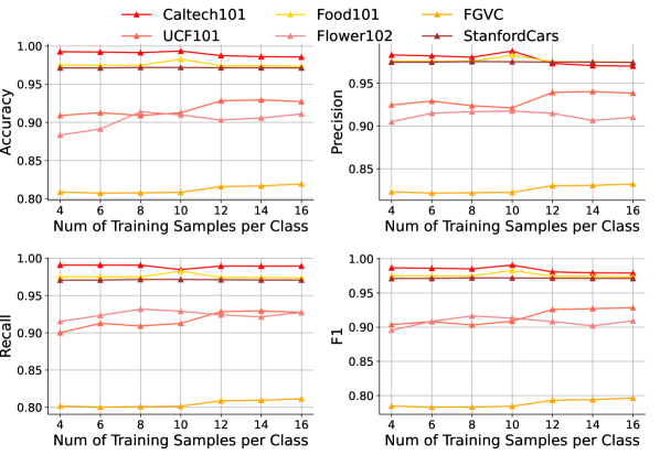
Figure 4: Robustness study w.r.t. number of training samples.

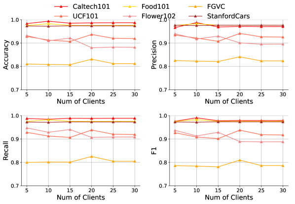
Figure 5: Scalability study w.r.t. number of clients.

Method	FedAvg (NN)	FedKA (NN)	PromptFL	FedTPG	FedCLIP	Fed-MP (ours)
time/img (s)	$0.0031$	$0.0031$	$0.0366$	$0.0367$	$0.0362$	$0.0369$
trainable params.	$100.00\%$	$100.00\%$	$0.0140\%$	$0.0549\%$	$0.2745\%$	$0.2783\%$

Table 3: Averaged processing time per image (in seconds) and ratio of trainable parameters (in percentage).

5.4 Robustness Study

In this section, we conduct a robustness study w.r.t. the number of training samples per class. This is a key factor affecting the finetuning quality. In particular, we change it from 2 to 16, and keep the number of clients as 10. The results are shown in Figure 4. We observe that Fed-MP is generally robust against the number of training samples. On Flower102 and FGVC, Fed-MP is relatively more sensitive to the number of training samples. This is because that different kinds of flowers and aircraft are more difficult to distinguish compared to food types and car makes.

5.5 Scalability Study

Then, we investigate the scalability of Fed-MP w.r.t. the number of clients, as the number of clients in an FL application is a key factor affecting data heterogeneity and training stability. Specifically, we use the same test classes in our 10-client setting as the test classes, but re-distribute the training classes to different number of clients (from 5 to 30). The results are shown in Figure 5. We observe that Fed-MP is scalable and achieves consistent high performance as the number of clients increases.

5.6 Efficiency Evaluation

Finally, we compare the averaged processing time per image (in seconds) and the ratio of trainable parameters (in percentage) among different methods. We show that Fed-MP is a light-weight and feasible solution for FL applications. From Table 3, we observe CLIP-based methods need more time to process image than NN-based methods. Moreover, by comparing the processing time per image across different methods, our Fed-MP is in general as fast as other CLIP-based baseline methods. In terms of memory saving, Fed-MP can be considered as a parameter-efficient method, because only less than 0.3% of the model parameters need to be trained, which is much fewer than FedTPG. However, we also acknowledge that Fed-MP needs to train more parameters than FedCLIP. This is expected, because Fed-MP uses the same adapter for the visual encoder as FedCLIP, but Fed-MP also trains the extra client residuals.

6 Conclusion

This work is the first to address the open-vocabulary challenge in FL applications. In particular, we present Fed-MP, a novel open-vocabulary FL framework that is tailored for finetuning VLMs for FL applications. Fed-MP provides an effective solution to make high-quality predictions for queries that involve novel unseen categories. Extensive experimental results on various datasets demonstrate the effectiveness of our method.

7 Limitations

One limitation of this work is that our method introduces extra hyperparameters. For different applications, one might need to finetune these hyperparameters, which brings extra computational cost. As for the actually trainable modules, there is only a small two-layer network and light-weight perturbations. Another limitation of this work is that our method does not take the inherent bias of the pre-trained VLM into account. However, it is known that the pre-trained foundation models usually have encoded the bias in the pre-training data (e.g., stereotypical data, racism and hate speech). Such bias could have negative ethical implications on downstream FL applications. Therefore, a future research direction is to develop a benign, fair, open-vocabulary FL framework.

Ethics Statement

Our work provides a data-efficient and privacy-aware solution to address the open-vocabulary problem in federated learning. Our method automatically generalizes to a new user and is capable of answering her/his queries that involve data from novel categories. In terms of real-world applications, with Fed-MP, the update frequency of the deployed FL model could be drastically reduced, and there is no need to collect huge amount of training data for novel classes. The above two advantages of Fed-MP reduce the risk of collecting private user data.

Appendix A: Implementation Details

Hyperparameters

For Fed-MP and all baseline methods that use CLIP, the learning rate is initialized as 1e-5. The learning rate for baseline methods that use ResNet-18 is 5e-4. The models are optimized via AdamW. The local training epoch is 2 and the global epoch is also 2. For all methods with key hyperparameters, we firstly performed grid search with the resolution of 0.1 until find the best performance. Based on that, we further reduce the search resolution to 0.01 until find best performance. In terms of the confidence threshold $\epsilon$, on Caltech101, UCF101, Flower102, we use $20\%$ of the maximum entropy given the distribution of the datasets on different clients. As for FGVC, Food101, we set $\epsilon$ equal to $3å0\%$ of maximum entropy. For StanfordCars, we used $10\%$. Our hardware is NVIDIA A40.

Baseline Implementation

We use ImageNet pre-trained ResNet-18 as the backbone model for FedAvg and FedKA. Upon implementation, we modify and re-train the classification head of the pre-trained ResNet-18 to fit it into our classification problem. Moreover, when performing aggregation and inference, these classification heads are not used, because they can not provide predictions for unseen classes. Therefore, we only aggregate the feature extraction modules of the finetuned ResNet-18 to obtain the global model. As for inference, we use the aggregated feature extractor to produce adapted representations. Using extracted representations, we further perform K-means clustering and linear sum assignment, to map the representations onto the unseen test classes. K-means and linear sum assignment is implemented using the SciPy library.

Evaluation Metrics

In Table 1, we use the scikit-learn library to compute the macro-averaged F1. Due to class imbalance, it is likely that F1 score is lower than precision and recall at the same time.

Implementation of Multimodal Prototyping

Finally, when implementing multimodal prototyping, we do not save all the visual prototypes for the sake of efficiency. Instead, we only dynamically update and save the centroid of each visual prototype set. For each class, this could be done with following steps:

• At time step $n$, the centroids of all prototypes are computed;

• Save the centroids and the number of prototypes used for each class;

• At the next time step $n+1$, if there is a new prototype added to the prototype set of a specific class $c$, then the sum of previous prototypes of will be reproduced by $\sum_{q\in Q_{c}}q=\bar{q}_{c}\cdot|Q_{c}|$;

• Update the new centroid of the visual prototype for class $c$: $\bar{q}_{c}=\frac{\sum_{Q_{c}}q+\frac{z^{\prime}}{||z^{\prime}||}}{|Q_{c}|+1}$.

Appendix A Appendix B: Overall Framework

1 Input CLIP image encoder $f_{I}$, CLIP text encoder $f_{T}$, adapter $f_{A}$, datasets of local clients $\mathcal{D}_{1},\mathcal{D}_{2},...,\mathcal{D}_{K}$;

2 Hyperparameters Learning rate; Initialize the visual adapter $f_{A}$ ;

3 Clients download $f_{I}$, $f_{T}$ and $f_{A}$ ;

4 for k=1,2,…,K do

5       Receive trainable models: $f^{(k)}_{A}=f_{A}$ ;

6       Initialize the client residual $\Delta^{(k)}$ ;

7       for local epochs do

8             Compute normal visual representations: $z=f_{I}(x)$ ;

9             Compute adapted visual representations: $z^{\prime}=z+f_{A}(z)$;

10             Compute normal text representations: $t=f_{T}(\texttt{A photo of [class c]})$ ;

11             Compute perturbed text representations: $t^{\prime}=t+\alpha\delta$;

12             Compute CLIP adaptation loss $\mathcal{L}_{adap}$ with Equation 5;

13             Update $f^{(k)}_{A}$ and $\Delta^{(k)}$ with gradient descent;

14       end for

15      Obtain perturbed text representations $\mathcal{T}^{{}^{\prime}(k)}$ by adding $\delta\in\Delta^{(k)}$ to $t$.

16 end for

17Output Send $f^{(k)}_{A}$ and $\mathcal{T}^{{}^{\prime}(k)}$ to the central server ;

Algorithm 1 Fed-MP (Training)

1 Input CLIP image encoder $f_{I}$, CLIP text encoder $f_{T}$, adapter weights $f^{(1)}_{A}$, $f^{(2)}_{A}$,…$f^{(K)}_{A}$, perturbed client text representations $\mathcal{T}^{{}^{\prime}(1)}$, $\mathcal{T}^{{}^{\prime}(2)}$,…,$\mathcal{T}^{{}^{\prime}(K)}$, test data $\mathcal{D}_{test}$, test prompts $\mathcal{T}_{test}$;

2 Hyperparameters Confidence threhold $\epsilon$; Compute the expected similarity between the test user and clients using Equation 8;

3 Obtain $f_{A}$ by aggregating the adapter weights using Equation 9;

4 Initialize the visual prototypes as empty sets ;

5 for $x$ $\in\mathcal{D}_{test}$ do

6       Compute the centroids for the visual prototypes with Equation 13;

7       Compute the prediction with Equation 12;

8       Update the corresponding visual prototype set using the original pseudo prediction and Equation 11;

9      

10 end for

11Output Predictions for $\mathcal{D}_{test}$ ;

Algorithm 2 Fed-MP (Inference)

References

- Bossard et al. (2014) Lukas Bossard, Matthieu Guillaumin, and Luc Van Gool. 2014. Food-101–mining discriminative components with random forests. In Computer Vision–ECCV 2014: 13th European Conference, Zurich, Switzerland, September 6-12, 2014, Proceedings, Part VI 13, pages 446–461. Springer.
- Changpinyo et al. (2017) Soravit Changpinyo, Wei-Lun Chao, and Fei Sha. 2017. Predicting visual exemplars of unseen classes for zero-shot learning. In Proceedings of the IEEE international conference on computer vision, pages 3476–3485.
- Che et al. (2023) Liwei Che, Jiaqi Wang, Yao Zhou, and Fenglong Ma. 2023. Multimodal federated learning: A survey. Sensors, 23(15):6986.
- Chen et al. (2023) Haokun Chen, Yao Zhang, Denis Krompass, Jindong Gu, and Volker Tresp. 2023. Feddat: An approach for foundation model finetuning in multi-modal heterogeneous federated learning. arXiv preprint arXiv:2308.12305.
- Deng et al. (2009) Jia Deng, Wei Dong, Richard Socher, Li-Jia Li, Kai Li, and Li Fei-Fei. 2009. Imagenet: A large-scale hierarchical image database. In 2009 IEEE conference on computer vision and pattern recognition, pages 248–255. Ieee.
- Fei-Fei et al. (2004) Li Fei-Fei, Rob Fergus, and Pietro Perona. 2004. Learning generative visual models from few training examples: An incremental bayesian approach tested on 101 object categories. In 2004 conference on computer vision and pattern recognition workshop, pages 178–178. IEEE.
- Guo et al. (2023a) Tao Guo, Song Guo, and Junxiao Wang. 2023a. pfedprompt: Learning personalized prompt for vision-language models in federated learning. In Proceedings of the ACM Web Conference 2023, pages 1364–1374.
- Guo et al. (2023b) Tao Guo, Song Guo, Junxiao Wang, Xueyang Tang, and Wenchao Xu. 2023b. Promptfl: Let federated participants cooperatively learn prompts instead of models-federated learning in age of foundation model. IEEE Transactions on Mobile Computing.
- He et al. (2016) Kaiming He, Xiangyu Zhang, Shaoqing Ren, and Jian Sun. 2016. Deep residual learning for image recognition. In Proceedings of the IEEE conference on computer vision and pattern recognition, pages 770–778.
- He et al. (2022) Rundong He, Zhongyi Han, Xiankai Lu, and Yilong Yin. 2022. Safe-student for safe deep semi-supervised learning with unseen-class unlabeled data. In Proceedings of the IEEE/CVF Conference on Computer Vision and Pattern Recognition, pages 14585–14594.
- Iwasawa and Matsuo (2021) Yusuke Iwasawa and Yutaka Matsuo. 2021. Test-time classifier adjustment module for model-agnostic domain generalization. Advances in Neural Information Processing Systems, 34:2427–2440.
- Jiang et al. (2022) Meirui Jiang, Zirui Wang, and Qi Dou. 2022. Harmofl: Harmonizing local and global drifts in federated learning on heterogeneous medical images. In Proceedings of the AAAI Conference on Artificial Intelligence, volume 36, pages 1087–1095.
- Krause et al. (2013) Jonathan Krause, Michael Stark, Jia Deng, and Li Fei-Fei. 2013. 3d object representations for fine-grained categorization. In Proceedings of the IEEE international conference on computer vision workshops, pages 554–561.
- Kuchibhotla et al. (2022) Hari Chandana Kuchibhotla, Sumitra S Malagi, Shivam Chandhok, and Vineeth N Balasubramanian. 2022. Unseen classes at a later time? no problem. In Proceedings of the IEEE/CVF Conference on Computer Vision and Pattern Recognition, pages 9245–9254.
- Li et al. (2023) Guanghao Li, Wansen Wu, Yan Sun, Li Shen, Baoyuan Wu, and Dacheng Tao. 2023. Visual prompt based personalized federated learning. arXiv preprint arXiv:2303.08678.
- Liu et al. (2021) Ming Liu, Stella Ho, Mengqi Wang, Longxiang Gao, Yuan Jin, and He Zhang. 2021. Federated learning meets natural language processing: A survey. arXiv preprint arXiv:2107.12603.
- Liu et al. (2020) Yang Liu, Anbu Huang, Yun Luo, He Huang, Youzhi Liu, Yuanyuan Chen, Lican Feng, Tianjian Chen, Han Yu, and Qiang Yang. 2020. Fedvision: An online visual object detection platform powered by federated learning. In Proceedings of the AAAI conference on artificial intelligence, volume 34, pages 13172–13179.
- Lu et al. (2023) Wang Lu, Xixu Hu, Jindong Wang, and Xing Xie. 2023. Fedclip: Fast generalization and personalization for clip in federated learning. arXiv preprint arXiv:2302.13485.
- Maji et al. (2013) Subhransu Maji, Esa Rahtu, Juho Kannala, Matthew Blaschko, and Andrea Vedaldi. 2013. Fine-grained visual classification of aircraft. arXiv preprint arXiv:1306.5151.
- McMahan et al. (2017) Brendan McMahan, Eider Moore, Daniel Ramage, Seth Hampson, and Blaise Aguera y Arcas. 2017. Communication-efficient learning of deep networks from decentralized data. In Artificial intelligence and statistics, pages 1273–1282. PMLR.
- Nilsback and Zisserman (2008) Maria-Elena Nilsback and Andrew Zisserman. 2008. Automated flower classification over a large number of classes. In 2008 Sixth Indian conference on computer vision, graphics & image processing, pages 722–729. IEEE.
- Qiu et al. (2023) Chen Qiu, Xingyu Li, Chaithanya Kumar Mummadi, Madan Ravi Ganesh, Zhenzhen Li, Lu Peng, and Wan-Yi Lin. 2023. Text-driven prompt generation for vision-language models in federated learning. arXiv preprint arXiv:2310.06123.
- Radford et al. (2021) Alec Radford, Jong Wook Kim, Chris Hallacy, Aditya Ramesh, Gabriel Goh, Sandhini Agarwal, Girish Sastry, Amanda Askell, Pamela Mishkin, Jack Clark, et al. 2021. Learning transferable visual models from natural language supervision. In International conference on machine learning, pages 8748–8763. PMLR.
- Shu et al. (2018) Lei Shu, Hu Xu, and Bing Liu. 2018. Unseen class discovery in open-world classification. arXiv preprint arXiv:1801.05609.
- Soomro et al. (2012) Khurram Soomro, Amir Roshan Zamir, and Mubarak Shah. 2012. Ucf101: A dataset of 101 human actions classes from videos in the wild. arXiv preprint arXiv:1212.0402.
- Sun et al. (2023) Yuwei Sun, Ng Chong, and Hideya Ochiai. 2023. Feature distribution matching for federated domain generalization. In Asian Conference on Machine Learning, pages 942–957. PMLR.
- Xu et al. (2022) An Xu, Wenqi Li, Pengfei Guo, Dong Yang, Holger R Roth, Ali Hatamizadeh, Can Zhao, Daguang Xu, Heng Huang, and Ziyue Xu. 2022. Closing the generalization gap of cross-silo federated medical image segmentation. In Proceedings of the IEEE/CVF Conference on Computer Vision and Pattern Recognition, pages 20866–20875.
- Yang et al. (2023) Fu-En Yang, Chien-Yi Wang, and Yu-Chiang Frank Wang. 2023. Efficient model personalization in federated learning via client-specific prompt generation. In Proceedings of the IEEE/CVF International Conference on Computer Vision, pages 19159–19168.
- Yu et al. (2023) Tao Yu, Zhihe Lu, Xin Jin, Zhibo Chen, and Xinchao Wang. 2023. Task residual for tuning vision-language models. In Proceedings of the IEEE/CVF Conference on Computer Vision and Pattern Recognition, pages 10899–10909.
- Zhang et al. (2023) Ruipeng Zhang, Qinwei Xu, Jiangchao Yao, Ya Zhang, Qi Tian, and Yanfeng Wang. 2023. Federated domain generalization with generalization adjustment. In Proceedings of the IEEE/CVF Conference on Computer Vision and Pattern Recognition, pages 3954–3963.
- Zhou et al. (2022) Kaiyang Zhou, Jingkang Yang, Chen Change Loy, and Ziwei Liu. 2022. Conditional prompt learning for vision-language models. In Proceedings of the IEEE/CVF conference on computer vision and pattern recognition, pages 16816–16825.