Adaptive hybrid high-order method for guaranteed lower eigenvalue bounds

Abstract.

The higher-order guaranteed lower eigenvalue bounds of the Laplacian in the recent work by Carstensen, Ern, and Puttkammer [Numer. Math. 149, 2021] require a parameter $C_{\mathrm{st},1}$ that is found not robust as the polynomial degree $p$ increases. This is related to the $H^{1}$ stability bound of the $L^{2}$ projection onto polynomials of degree at most $p$ and its growth $C_{\rm st,1}\propto(p+1)^{1/2}$ as $p\to\infty$. A similar estimate for the Galerkin projection holds with a $p$-robust constant $C_{\mathrm{st},2}$ and $C_{\mathrm{st},2}\leq 2$ for right-isosceles triangles. This paper utilizes the new inequality with the constant $C_{\mathrm{st},2}$ to design a modified hybrid high-order (HHO) eigensolver that directly computes guaranteed lower eigenvalue bounds under the idealized hypothesis of exact solve of the generalized algebraic eigenvalue problem and a mild explicit condition on the maximal mesh-size in the simplicial mesh. A key advance is a $p$-robust parameter selection.

The analysis of the new method with a different fine-tuned volume stabilization allows for a priori quasi-best approximation and improved $L^{2}$ error estimates as well as a stabilization-free reliable and efficient a posteriori error control. The associated adaptive mesh-refining algorithm performs superior in computer benchmarks with striking numerical evidence for optimal higher empirical convergence rates.

1. Introduction

This paper proposes and analyzes a new hybrid high-order (HHO) eigensolver for the direct computation of guaranteed lower eigenvalue bounds (GLB) for the Laplacian.

1.1. Three categories of GLB

The min-max principle enables guaranteed upper eigenvalue bounds but prevents a direct computation of a GLB by a conforming approximation in a Rayleigh quotient. So GLB shall be based on nonconforming finite element methods (FEM), on modified mass and/or stiffness matrices (with reduced integration or fine-tuned stabilization terms), or on further post-processing. The last decade has seen a few GLB we group in three categories (i)–(iii).

1. The a posteriori error analysis for symmetric second-order elliptic eigenvalue problems started with [54, 43, 35] under the (unverified) hypothesis of a sufficiently small mesh-size. With additional a priori information on spectral gaps, the latest a posteriori post-processings [15, 14, 13] provide GLB.

2. Classical nonconforming FEM [20, 22, 45] and mixed FEM [39] allow for the GLB $\lambda_{h}/(1+\delta\lambda_{h})\leq\lambda$ with the discrete eigenvalue $\lambda_{h}$ and a known parameter $\delta\propto h_{\max}^{2}$ in terms of the maximal mesh-size $h_{\max}$. On the positive side, the GLB provides unconditional information on the exact eigenvalue $\lambda$ from the computed discrete eigenvalue $\lambda_{h}$. On the negative side, the global parameter $h_{\max}$ can spoil a very accurate approximation $\lambda_{h}$ in this GLB and is of lowest-order only. A fine-tuned stabilization of the classical nonconforming FEM in [23], however, provides a first (but low-order) remedy of the third category.

3. Higher-order hybrid discontinuous Galerkin (HDG) or HHO discretizations [25, 19] can compute direct GLB $\lambda_{h}\leq\lambda$ under the sufficient condition (e.g., in [19] for the HHO method and the Laplacian)

   (1.1) $$\sigma_{1}^{2}\beta+\kappa^{2}h_{\max}^{2}\min\{\lambda,\lambda_{h}\}\leq\alpha$$

   with (universal or computed) constants $\sigma_{1},\kappa$ and known parameters $0<\alpha<1,0<\beta<\infty$ (selected in the discrete scheme). If the exact Dirichlet eigenvalue $\lambda$ of number $j\in\mathbb{N}_{0}$ of the Laplace operator and the corresponding discrete eigenvalue $\lambda_{h}$ satisfy (1.1), then $\lambda_{h}\leq\lambda$ is a GLB. The two-fold use of (1.1) is a priori or a posteriori. First, given an upper bound $\mu\geq\lambda>0$ of $\lambda$ (e.g., by some conforming approximation or post-processing), (1.1) provides an upper bound $h_{\max}^{2}\leq(\alpha-\sigma_{1}^{2}\beta)/(\kappa^{2}\mu)$ for the maximal initial mesh-size. This condition is sufficient for (1.1) and guarantees a priori that $\lambda_{h}\leq\lambda$. Second, (1.1) may be checked a posteriori for any computed value $\lambda_{h}$. Then $\sigma_{1}^{2}\beta+\kappa^{2}h_{\max}^{2}\lambda_{h}\leq\alpha$ implies (1.1) and so, $\lambda_{h}\leq\lambda$.

This paper presents a new HHO eigensolver of the third category.

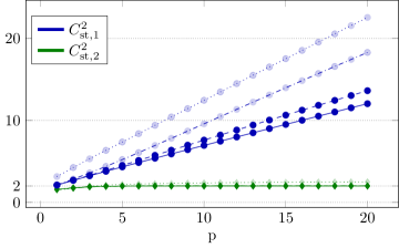
Figure 1. Approximations of $C_{\rm st,1}^{2}$ and $C_{\rm st,2}^{2}$ as a function of the polynomial degree $p$ on the equilateral triangle , the right-isosceles triangle , $\coloneqq\mathrm{conv}\{(0,0),(1.5,0),(0,1)\}$, and $\coloneqq\mathrm{\{}(0,0),(1,0),(-1/2,1)\}$.

1.2. Motivation and outline of Section 2

The constants $\sigma_{1}^{2}\coloneqq C_{\textrm{st,1}}^{2}-1$ and $\kappa\coloneqq C_{P}C_{\textrm{st,1}}$ in (1.1) depend on the Poincaré constant $C_{P}\leq 1/\pi$ and a stability constant $C_{\textrm{st,1}}$. The latter has to be contrasted with the constant $C_{\rm st,2}$, where $C_{\rm st,1}$ and $C_{\rm st,2}$ are the best possible constants in the stability estimates

(1.2) $$\|\nabla(1-\Pi_{p+1})f\|_{L^{2}(T)} \leq C_{\textrm{st,1}}\|(1-\Pi_{p})\nabla f\|_{L^{2}(T)}\quad\text{for all }f\in H^{1}(T),$$

(1.3) $$\|\nabla(1-G_{p+1})f\|_{L^{2}(T)} \leq C_{\textrm{st,2}}\|(1-\Pi_{p})\nabla f\|_{L^{2}(T)}\quad\text{for all }f\in H^{1}(T)$$

in a given simplex $T\subset\mathbb{R}^{n}$ with the (component-wise) $L^{2}$ projection $\Pi_{m}$ and the Galerkin projection $G_{m}$ onto polynomials of total degree at most $m\in\mathbb{N}_{0}$. The two constants $C_{\mathrm{st,1}}$ and $C_{\mathrm{st,2}}$ are independent of the diameter $h_{T}\coloneqq\mathrm{diam}(T)$ of $T$, but might depend on the shape of $T$ and the polynomial degree $p$. Figure 1 illustrates the behaviour of $C_{\rm st,1}$ and $C_{\rm st,2}$ for different triangular shapes and various polynomial degrees $p$. Section 2 investigates the $p$-robustness of $C_{\rm st,2}$ and reveals that $C_{\rm st,2}\leq C_{\rm st,1}\propto\sqrt{p+1}$ tends to infinity as $p\to\infty$, while we conjecture $C_{\rm st,2}\leq\sqrt{2}$ for triangles $T$ with maximum interior angle $\omega\leq\pi/2$. Notice that a large constant $C_{\mathrm{st,1}}$ leads to a large $\sigma_{1}$ in (1.1) and so, $\alpha<1$ enforces small $\beta$ and restricts the GLB to very fine meshes. The main motivation of this work arises from the convenient bound $C_{\rm st,2}\leq\sqrt{2}$: Can we design a discretization method of the third category (iii) based on $\sigma_{2}\coloneqq C_{P}C_{\textrm{st,2}}\leq\sqrt{2}/\pi$ in (1.1)?

1.3. A modified HHO method and outline of Section 3

This paper provides an affirmative answer with a new fine-tuned stabilization in a modified HHO scheme in Section 3 and a new criterion

(1.4) $$\sigma_{2}^{2}\max\{\beta,h_{\max}^{2}\min\{\lambda,\lambda_{h}\}\}\leq\alpha$$

sufficient for the GLB $\lambda_{h}\leq\lambda$. One advantage of (1.4) over (1.1) is the straight-forward and $p$-robust parameter selection $\beta\coloneqq\alpha/\sigma_{2}^{2}$. It turns out that $\sigma_{2}\leq\kappa$ and so (1.4) improves on (1.1) in the sense that $\sigma_{2}^{2}h_{\max}^{2}\lambda\leq\alpha$ holds on much coarser triangulations for higher polynomial degrees $p$.

Given a bounded polyhedral Lipschitz domain $\Omega\subset\mathbb{R}^{n}$, let $V\coloneqq H^{1}_{0}(\Omega)$ denote the Sobolev space endowed with the energy scalar product $a(u,v)\coloneqq(\nabla u,\nabla v)_{L^{2}(\Omega)}$ and the $L^{2}$ scalar product $b(u,v)\coloneqq(u,v)_{L^{2}(\Omega)}$ for all $u,v\in V$. This paper considers the model problem that seeks an eigenpair $(\lambda,u)\in\mathbb{R}_{+}\times(V\setminus\{0\})$ such that

(1.5) $$a(u,v)=\lambda b(u,v)\text{ for any }v\in V.$$

The HHO methodology has been introduced in [32, 31] and is related to HDG and nonconforming virtual element methods [27]. Given a regular triangulation $\mathcal{T}$ into simplices, the ansatz space $V_{h}=P_{p+1}(\mathcal{T})\times P_{p}(\mathcal{F}(\Omega))$ consists of piecewise polynomials of (total) degree at most $p+1$ attached to the simplices and piecewise polynomials of degree at most $p$ attached to the interior faces. Two reconstruction operators link the two components of $v_{h}\in V_{h}$: The potential reconstruction $\mathcal{R}v_{h}\in P_{p+1}(\mathcal{T})$ provides a discrete approximation to $v$ in the space of piecewise polynomials $P_{p+1}(\mathcal{T})$ of degree at most $p+1$. The gradient reconstruction $\mathcal{G}v_{h}\in\mathrm{RT}_{p}^{\mathrm{pw}}(\mathcal{T})$ approximates the gradient $\nabla v$ in the space of piecewise Raviart-Thomas functions $\mathrm{RT}_{p}^{\mathrm{pw}}(\mathcal{T})$ [1, 30]. Let $Sv_{h}\coloneqq v_{\mathcal{T}}-\mathcal{R}v_{h}\in P_{p+1}(\mathcal{T})$ for any $v_{h}=(v_{\mathcal{T}},v_{\mathcal{F}})\in V_{h}$ denote the additional cell-based stabilization. Given positive parameters $0<\alpha<1$ and $0<\beta<\infty$, the bilinear forms $a_{h}:V_{h}\times V_{h}\to\mathbb{R}$ and $b_{h}:V_{h}\times V_{h}\to\mathbb{R}$ read

(1.6) $$a_{h}(u_{h},v_{h}) \coloneqq(\mathcal{G}u_{h},\mathcal{G}v_{h})_{L^{2}(\Omega)}-\alpha((1-\Pi_{p})\mathcal{G}u_{h},(1-\Pi_{p})\mathcal{G}v_{h})_{L^{2}(\Omega)}$$

$$\qquad+\beta(h_{\mathcal{T}}^{-2}Su_{h},Sv_{h})_{L^{2}(\Omega)},$$

(1.7) $$b_{h}(u_{h},v_{h}) \coloneqq(u_{\mathcal{T}},v_{\mathcal{T}})_{L^{2}(\Omega)}\text{ for any }u_{h}=(u_{\mathcal{T}},u_{\mathcal{F}}),v_{h}=(v_{\mathcal{T}},v_{\mathcal{F}})\in V_{h}.$$

The discrete eigenvalue problem seeks $(\lambda_{h},u_{h})\in\mathbb{R}^{+}\times(V_{h}\setminus\{0\})$ with

(1.8) $$a_{h}(u_{h},v_{h})=\lambda_{h}b_{h}(u_{h},v_{h})\text{ for all }v_{h}\in V_{h}.$$

The definitions of $\mathcal{R}$, $\mathcal{G}$, and further details follow in Section 3 below.

1.4. GLB with $p$-robust parameters and outline of Section 4

The discrete bilinear form $a_{h}$ from [19] with parameter $C_{\rm st,1}\propto\sqrt{p+1}$ utilizes the different stabilization $\beta(\nabla_{\mathrm{pw}}Su_{h},\nabla_{\mathrm{pw}}Sv_{h})_{L^{2}(\Omega)}$ instead of $\beta(h_{\mathcal{T}}^{-2}Su_{h},Sv_{h})_{L^{2}(\Omega)}$ in (1.6). The two stabilizations are locally equivalent, but the innovative difference is that the parameter selection in the new scheme circumvents an inverse inequality, and rather builds it into the scheme. Section 4 verifies the sufficient condition (1.4) for exact GLB under the assumption of exact solve.

1.5. A priori error analysis of the new scheme and outline of Section 5

A quasi-best approximation for the source problem [38] allows for quasi-best approximation results in Theorem 5.1 for a simple eigenvalue $\lambda$, namely

$$|\lambda-\lambda_{h}|+a_{h}(\mathrm{I}u-u_{h},\mathrm{I}u-u_{h})+h_{\max}^{-2s}\|u-u_{\mathcal{T}}\|_{L^{2}(\Omega)}^{2}$$

(1.9) $$\leq C_{\ref{cnst:best-approximation}}\min_{v_{p+1}\in P_{p+1}(\mathcal{T})}\|\nabla_{\mathrm{pw}}(u-v_{p+1})\|_{L^{2}(\Omega)}^{2}$$

with a positive constant $C_{1}$ and the minimum $0<s\leq 1$ of the index of elliptic regularity and one; the HHO interpolation $\mathrm{I}:V\to V_{h}$ is recalled in Subsection 3.3 below. Compared to earlier results in [12, 19], (1.9) provides an additional positive power $s$ of $h_{\max}$ in the $L^{2}$ error. This is important as it eventually enables the absorption of higher-order terms in the a posteriori error analysis.

1.6. Stabilization-free a posteriori error analysis and outline of Section 6

Let $p_{h}\coloneqq\Pi_{p}\mathcal{G}u_{h}\in P_{p}(\mathcal{T};\mathbb{R}^{n})$ denote the $L^{2}$ projection of the gradient reconstruction $\mathcal{G}u_{h}\in\mathrm{RT}_{p}^{\mathrm{pw}}(\mathcal{T})$ onto the space of vector-valued piecewise polynomials $P_{p}(\mathcal{T};\mathbb{R}^{n})$. For any $T\in\mathcal{T}$ of volume $|T|$, define

(1.10) $$\eta^{2}(T)\coloneqq|T|^{2/n}\big{(}\|\mathrm{div}\,p_{h}+\lambda_{h}u_{\mathcal{T}}\|_{L^{2}(T)}^{2}+\|\mathrm{curl}\,p_{h}\|^{2}_{L^{2}(T)}\big{)}$$

$$\quad+|T|^{1/n}\Big{(}\sum_{F\in\mathcal{F}(T)\cap\mathcal{F}(\Omega)}\|[p_{h}\cdot\nu_{F}]_{F}\|_{L^{2}(F)}^{2}+\sum_{F\in\mathcal{F}(T)}\|[p_{h}\times\nu_{F}]_{F}\|_{L^{2}(F)}^{2}\Big{)}$$

with the normal jump $[p_{h}\cdot\nu_{F}]_{F}$ and the tangential jump $[p_{h}\times\nu_{F}]_{F}$ of $p_{h}$ across a side $F$ of $T$. Theorem 6.1 asserts reliability and efficiency of the error estimator $\eta^{2}\coloneqq\sum_{T\in\mathcal{T}}\eta^{2}(T)$ for sufficiently small mesh-sizes $h_{\max}$ in the sense that

(1.11) $$C_{\mathrm{eff}}^{-1}\eta\leq|\lambda-\lambda_{h}|+a_{h}(\mathrm{I}u-u_{h},\mathrm{I}u-u_{h})+\|\nabla u-p_{h}\|^{2}_{L^{2}(\Omega)}\leq C_{\mathrm{rel}}\eta.$$

1.7. Adaptive mesh-refining algorithm and outline of Section 7

Three 2D computer experiments in Section 7 provide striking numerical evidence that the criterion (1.4) indeed leads to confirmed lower eigenvalue bounds. The adaptive mesh-refining algorithm driven by the refinement indicator $\eta$ from (1.10) recovers the optimal convergence rates of the eigenvalue error $\lambda-\lambda_{h}$ in all numerical benchmarks with singular eigenfunctions. This is the first time that $p$-robust higher-order GLB of the third category are displayed.

1.8. General notation

Standard notation for Lebesgue and Sobolev function spaces applies throughout this paper. In particular, $(\bullet,\bullet)_{L^{2}(\omega)}$ denotes the $L^{2}$ scalar product and $H(\mathrm{div},\omega)$ is the space of Sobolev functions with weak divergence in $L^{2}(\omega)$ for a domain $\omega\subset\mathbb{R}^{n}$. Recall the abbreviation $V\coloneqq H^{1}_{0}(\Omega)$ for the space of Sobolev functions, endowed with the energy scalar product $a(u,v)\coloneqq(\nabla u,\nabla v)_{L^{2}(\Omega)}$ and the $L^{2}$ scalar product $b(u,v)\coloneqq(u,v)_{L^{2}(\Omega)}$ for all $u,v\in V$.

For a subset $M\subset\mathbb{R}^{n}$ of diameter $h_{M}$, let $P_{p}(M)$ denote the space of polynomials of maximal (total) degree $p$ regarded as functions defined in $M$. Given a simplex $T\subset\mathbb{R}^{n}$, the space of Raviart-Thomas finite element functions reads

$$\mathrm{RT}_{p}(T) \coloneqq P_{p}(T;\mathbb{R}^{n})+xP_{p}(T)\subset P_{p+1}(T;\mathbb{R}^{n}).$$

The Galerkin projection $G\coloneqq G_{p+1}:H^{1}(T)\to P_{p+1}(T)$ maps $f\in H^{1}(T)$ to the unique solution $Gf$ to $\Pi_{0}Gf=\Pi_{0}f$ and

(1.12) $$(\nabla Gf,\nabla p_{p+1})_{L^{2}(T)}=(\nabla f,\nabla p_{p+1})_{L^{2}(T)}\text{ for all }p_{p+1}\in P_{p+1}(T)$$

with the convention $H^{1}(T)\coloneqq H^{1}(\mathrm{int}(T))$ for the interior $\mathrm{int}(T)=T^{\circ}$ of $T$. The Poincaré constant $C_{P}$ bounds $\|(1-\Pi_{0})f\|_{L^{2}(T)}\leq C_{P}h_{T}\|\nabla f\|_{L^{2}(T)}$ for all $f\in H^{1}(T)$. In 2D, $C_{P}\leq 1/j_{11}=0.260980$ with the first positive root of the Bessel function $J_{1}$ [44] and $C_{P}\leq 1/\pi$ in any space dimension [49, 5]. The context-sensitive notation $|\bullet|$ may denote the absolute value of a scalar, the Euclidean norm of a vector, the length of a side, or the volume of a simplex. The notation $A\lesssim B$ abbreviates $A\leq CB$ for a generic constant $C$ independent of the mesh-size and $A\approx B$ abbreviates $A\lesssim B\lesssim A$. Throughout this paper, $C_{1},\dots,C_{\ref{cnst:a-posteriori-absorption-small-mesh-size}}$ denote positive constants independent of the mesh-size.

2. Stability estimates

This section discusses the behaviour of the constants $C_{\rm st,1},C_{\rm st,2}$ from (1.2)–(1.3) as $p\to\infty$ and the computation of $\sigma_{2}\coloneqq C_{P}C_{\rm st,2}$ with the Poincaré constant $C_{P}$ in (1.4) that arises from the stability estimates in Lemma 2.2 below.

2.1. Stability constants and estimates

The following theorem asserts that $C_{\rm st,2}$ is $p$-robust (and small in general, see Figure 1) whereas $C_{\rm st,1}\to\infty$ as $p\to\infty$.

Theorem 2.1.

For any simplex $T$, there exist positive constants $1\leq C_{\rm st,2}\leq C_{\rm st,1}$ independent of the diameter $h_{T}$ such that (1.2)–(1.3) hold. In $n=2,3$ space dimensions, $C_{\rm st,1}\approx\sqrt{p+1}$ and $C_{\rm st,2}\approx 1$ as $p\to\infty$.

Proof.

The existence of the constants $1\leq C_{\rm st,1}\leq C_{\rm st,2}$ follows from [25, Theorem 3.1]; cf. Appendix A for further details. The technical proof of the $p$-robustness of $C_{\mathrm{st,2}}$ involves a linear bounded operator $R^{\mathrm{curl}}:H^{-1}(T;\mathbb{R}^{3})\to L^{2}(T;\mathbb{R}^{3})$ from [42, 28, 46] and is carried out in Appendix B. The robustness holds for $n=2$ with a simpler and hence omitted proof. The remaining parts of this proof concern the growth of $C_{\rm st,1}$. Let $X\coloneqq H^{1}(T)/\mathbb{R}$ denote the Hilbert space with inner product $(\nabla\bullet,\nabla\bullet)_{L^{2}(T)}$ and note that $\mathrm{ker}(\nabla(1-\Pi_{p+1}))=\mathrm{ker}((1-\Pi_{p})\nabla)=P_{p+1}(T)$. Since $\|(1-\Pi_{p})\nabla\phi\|_{L^{2}(T)}\leq{\left|\kern-1.07639pt\left|\kern-1.07639pt\left|\phi\right|\kern-1.07639pt\right|\kern-1.07639pt\right|}$ for every $\phi\in X$, the definition of the operator norm of the oblique projection $1-\Pi_{p+1}\in L(X;X)$ provides

$$\|1-\Pi_{p+1}\|\coloneqq\sup_{\phi\in X\setminus\{0\}}\frac{{\left|\kern-1.07639pt\left|\kern-1.07639pt\left|(1-\Pi_{p+1})\phi\right|\kern-1.07639pt\right|\kern-1.07639pt\right|}}{{\left|\kern-1.07639pt\left|\kern-1.07639pt\left|\phi\right|\kern-1.07639pt\right|\kern-1.07639pt\right|}}\leq\sup_{\phi\in X\setminus P_{p+1}(T)}\frac{{\left|\kern-1.07639pt\left|\kern-1.07639pt\left|(1-\Pi_{p+1})\phi\right|\kern-1.07639pt\right|\kern-1.07639pt\right|}}{\|(1-\Pi_{p})\nabla\phi\|_{L^{2}(T)}}=C_{\rm st,1}.$$

Kato’s oblique projection lemma [52] for the Hilbert space $X$ leads to $\|\Pi_{p+1}\|=\|1-\Pi_{p+1}\|\,\leq\,C_{\rm st,1}$ and $(1-\Pi_{p+1})G=0$ in $X$ for the Galerkin projection $G$ shows

$${\left|\kern-1.07639pt\left|\kern-1.07639pt\left|(1-\Pi_{p+1})f\right|\kern-1.07639pt\right|\kern-1.07639pt\right|}={\left|\kern-1.07639pt\left|\kern-1.07639pt\left|(1-\Pi_{p+1})(1-G)f\right|\kern-1.07639pt\right|\kern-1.07639pt\right|}\leq\|\Pi_{p+1}\|\;{\left|\kern-1.07639pt\left|\kern-1.07639pt\left|(1-G)f\right|\kern-1.07639pt\right|\kern-1.07639pt\right|} \text{for any }f\in X.$$

Since ${\left|\kern-1.07639pt\left|\kern-1.07639pt\left|(1-G)f\right|\kern-1.07639pt\right|\kern-1.07639pt\right|}\leq C_{\rm st,2}\|(1-\Pi_{p})\nabla f\|_{L^{2}(T)}$ from (1.3), this proves $\|\Pi_{p+1}\|\leq C_{\rm st,1}\leq C_{\rm st,2}\|\Pi_{p+1}\|$. The growth $\|\Pi_{p+1}\|\approx\sqrt{p+1}$ is known for tensor-product domains and also holds for simplices in $n=2,3$ dimensions; see [55] and [47, Sec. 5] for $\|\Pi_{p+1}\|\lesssim\sqrt{p+1}$ and Appendix C for the proof of $\sqrt{p+1}\lesssim\|\Pi_{p+1}\|$. ∎

The Poincaré inequality with the Poincaré constant $C_{P}$ and (1.3) with $C_{\rm st,2}\approx 1$ lead to a $p$-robust stability estimate with $\sigma_{2}\coloneqq C_{P}C_{\rm st,2}$.

Lemma 2.2 ($p$-robust stability).

Any $f\in H^{1}(T)$, $T$ a simplex, and $p\in\mathbb{N}_{0}$ satisfy

(2.1) $$\|h_{T}^{-1}(1-G)f\|_{L^{2}(T)} \leq\sigma_{2}\|(1-\Pi_{p})\nabla f\|_{L^{2}(T)}.\qed$$

2.2. Numerical comparison and conjecture

The following theorem considers the computation of guaranteed upper bounds of $C_{\rm st,2}$ in $n=2,3$ space dimensions for a control of $\sigma_{2}$ in (2.1).

$p$	$C_{\mathrm{st,2}}^{2}$	$p$	$C_{\mathrm{st,2}}^{2}$
$1$	1.59707221	$6$	1.99368122
$2$	1.75	$7$	1.99787853
$3$	1.91060394	$8$	1.99911016
$4$	1.95679115	$9$	1.99969758
$5$	1.98559893	$10$	1.99987656

Table 1. The constant $C_{\mathrm{st,2}}=m_{p}$ on right-isosceles triangles.

Given $v\in H^{1}(T;\mathbb{R}^{n})$ and $w\in H^{1}(T;\mathbb{R}^{2n-3})$, let $\mathrm{curl}\,v\coloneqq\partial_{1}v_{2}-\partial_{2}v_{1}$ and $\mathrm{Curl}\,w\coloneqq(\partial_{2}w,-\partial_{1}w)^{t}$ for $n=2$ and $\mathrm{curl}\,v\coloneqq(\partial_{2}v_{3}-\partial_{3}v_{2},\partial_{3}v_{1}-\partial_{1}v_{3},\partial_{1}v_{2}-\partial_{2}v_{1})^{t}$ and $\mathrm{Curl}\,w\coloneqq\mathrm{curl}\,w$ for $n=3$. For any $g\in H^{-1}(T;\mathbb{R}^{2n-3})$ in the dual space of $H^{1}_{0}(T;\mathbb{R}^{2n-3})$ endowed with the operator norm ${\left|\kern-1.07639pt\left|\kern-1.07639pt\left|\bullet\right|\kern-1.07639pt\right|\kern-1.07639pt\right|}_{*}$, let $(-\Delta)^{-1}g\in H^{1}_{0}(T;\mathbb{R}^{2n-3})$ denote the weak solution to $-\Delta v=g$ in $T$ componentwise with ${\left|\kern-1.07639pt\left|\kern-1.07639pt\left|g\right|\kern-1.07639pt\right|\kern-1.07639pt\right|}_{*}={\left|\kern-1.07639pt\left|\kern-1.07639pt\left|(-\Delta)^{-1}g\right|\kern-1.07639pt\right|\kern-1.07639pt\right|}$.

The gradients $\nabla P_{p+1}(T)$ of polynomials $P_{p+1}(T)$ of degree at most $p+1$ form a subspace of $P_{p}(T;\mathbb{R}^{n})$ and give rise to the $L^{2}$ orthogonal decomposition $P_{p}(T;\mathbb{R}^{n})=Q_{p}\oplus\nabla P_{p+1}(T)$ with $Q_{p}\perp\nabla P_{p+1}(T)$ in $L^{2}(T;\mathbb{R}^{n})$. Let $\mathrm{P}:P_{p}(T;\mathbb{R}^{n})\to\nabla P_{p+1}(T)$ denote the $L^{2}$ orthogonal projection onto $\nabla P_{p+1}(T)\subset P_{p}(T;\mathbb{R}^{n})$. The bilinear forms $\mathfrak{a}:Q_{p}\times Q_{p}\to\mathbb{R}$ and $\mathfrak{b}:Q_{p}\times Q_{p}\to\mathbb{R}$ are defined, for any $q_{p},r_{p}\in Q_{p}$, by

(2.2) $$\mathfrak{a}(q_{p},r_{p})\coloneqq(q_{p},r_{p})_{L^{2}(T)}\quad\text{and}\quad\mathfrak{b}(q_{p},r_{p})\coloneqq((-\Delta)^{-1}\mathrm{curl}\,q_{p},\mathrm{curl}\,r_{p})_{L^{2}(T)}.$$

Theorem 2.3 (stability constant).

The maximal eigenvalue

(2.3) $$m_{p}^{2}\coloneqq\max_{\begin{subarray}{c}q_{p}\in P_{p}(T;\mathbb{R}^{n})\\ \mathrm{curl}\,q_{p}\neq 0\end{subarray}}\min_{v_{p+1}\in P_{p+1}(T)}\|q_{p}-\nabla v_{p+1}\|_{L^{2}(T)}^{2}/{\left|\kern-1.07639pt\left|\kern-1.07639pt\left|\mathrm{curl}\,q_{p}\right|\kern-1.07639pt\right|\kern-1.07639pt\right|}_{*}^{2}$$

of the eigenvalue problem

(2.4) $$\mathfrak{a}(q_{p},r_{p})=\lambda\mathfrak{b}(q_{p},r_{p})\quad\text{for all }r_{p}\in Q_{p}$$

leads to the upper bound $C_{\mathrm{st,2}}\leq\max\{1,m_{p}C_{n}\}$ for $C_{2}=1$ and $C_{3}=2/\sqrt{3}$.

Notice that (2.4) is a finite-dimensional eigenvalue problem and $(-\Delta)^{-1}q_{p}$ in $\mathfrak{b}(q_{p},r_{p})$ can be approximated by, e.g., a conforming FEM. Numerical experiments below even suggest that the bound $C_{\rm st,2}=m_{p}$ is exact in $n=2$ dimensions.

Proof.

If $p=0$, $\nabla P_{1}(T)=P_{0}(T;\mathbb{R}^{n})$ implies $\nabla Gf=\Pi_{0}\nabla f$ for all $f\in H^{1}(T)$, whence $C_{\mathrm{st,2}}=1$. The remaining parts of the proof therefore assume $p\geq 1$. Given $f\in H^{1}(T)$, assume without loss of generality that $\nabla f\perp\nabla P_{p+1}(T)$ in $L^{2}(T;\mathbb{R}^{n})$ (otherwise substitute $g\coloneqq f-Gf$ and observe that $\|(1-\Pi_{p})\nabla f\|_{L^{2}(T)}=\|(1-\Pi_{p})\nabla g\|_{L^{2}(T)}$). Throughout this proof, abbreviate $q_{p}\coloneqq\Pi_{p}\nabla f\in P_{p}(T;\mathbb{R}^{n})$. A Helmholtz decomposition leads to $q_{p}=\nabla a+\mathrm{Curl}\,b$ with $a\in H^{1}(T)$ and $b\in H^{1}_{0}(T;\mathbb{R}^{2n-3})$. For any $v\in H^{1}_{0}(T;\mathbb{R}^{2n-3})$, the $L^{2}$ orthogonality $\mathrm{Curl}\,v\perp\nabla a$ in $L^{2}(T;\mathbb{R}^{n})$, an integration by parts, and a Cauchy inequality prove

$$\int_{T}v\cdot\mathrm{curl}\,q_{p}\,\mathrm{d}x =\int_{T}q_{p}\cdot\mathrm{Curl}\,v\,\mathrm{d}x$$

(2.5) $$=\int_{T}\mathrm{Curl}\,b\cdot\mathrm{Curl}\,v\,\mathrm{d}x\leq\|\mathrm{Curl}\,b\|_{L^{2}(T)}\|\mathrm{Curl}\,v\|_{L^{2}(T)}.$$

In 2D, $\|\mathrm{Curl}\,v\|_{L^{2}(\Omega)}={\left|\kern-1.07639pt\left|\kern-1.07639pt\left|v\right|\kern-1.07639pt\right|\kern-1.07639pt\right|}$ and in 3D, $\|\mathrm{Curl}\,v\|_{L^{2}(\Omega)}\leq 2{\left|\kern-1.07639pt\left|\kern-1.07639pt\left|v\right|\kern-1.07639pt\right|\kern-1.07639pt\right|}/\sqrt{3}$. (The proof solely involves elementary algebra and is therefore omitted.) Hence, (2.5) implies

(2.6) $${\left|\kern-1.07639pt\left|\kern-1.07639pt\left|\mathrm{curl}\,q_{p}\right|\kern-1.07639pt\right|\kern-1.07639pt\right|}_{*}=\sup_{v\in H^{1}_{0}(T;\mathbb{R}^{2n-3})\setminus\{0\}}\int_{T}v\cdot\mathrm{curl}\,q_{p}\,\mathrm{d}x/{\left|\kern-1.07639pt\left|\kern-1.07639pt\left|v\right|\kern-1.07639pt\right|\kern-1.07639pt\right|}\leq C_{n}\|\mathrm{Curl}\,b\|_{L^{2}(T)}.$$

(Notice that ${\left|\kern-1.07639pt\left|\kern-1.07639pt\left|q_{p}\right|\kern-1.07639pt\right|\kern-1.07639pt\right|}_{*}=\|\mathrm{Curl}\,b\|_{L^{2}(T)}={\left|\kern-1.07639pt\left|\kern-1.07639pt\left|b\right|\kern-1.07639pt\right|\kern-1.07639pt\right|}$ in 2D). Since $\nabla P_{p+1}(T)\subset P_{p}(T;\mathbb{R}^{n})$, the best approximation of $q_{p}$ in $\nabla P_{p+1}(T)$ satisfies the $L^{2}$ orthogonality $q_{p}\perp\nabla P_{p+1}(T)$. This and the Pythagoras theorem provide

$$\min_{v_{p+1}\in P_{p+1}(T)}\|q_{p}-\nabla v_{p+1}\|_{L^{2}(T)}^{2}=\|q_{p}\|_{L^{2}(T)}^{2}={\left|\kern-1.07639pt\left|\kern-1.07639pt\left|a\right|\kern-1.07639pt\right|\kern-1.07639pt\right|}^{2}+\|\mathrm{Curl}\,b\|_{L^{2}(T)}^{2}.$$

On the other hand, the constant $m_{p}$ from (2.3) satisfies

$$\min_{v_{p+1}\in P_{p+1}(T)}\|q_{p}-\nabla v_{p+1}\|_{L^{2}(T)}^{2}\leq m_{p}^{2}{\left|\kern-1.07639pt\left|\kern-1.07639pt\left|\mathrm{curl}\,q_{p}\right|\kern-1.07639pt\right|\kern-1.07639pt\right|}_{*}^{2}.$$

Hence, (2.6) implies

(2.7) $${\left|\kern-1.07639pt\left|\kern-1.07639pt\left|a\right|\kern-1.07639pt\right|\kern-1.07639pt\right|}^{2}\leq(m_{p}^{2}C_{n}^{2}-1)\|\mathrm{Curl}\,b\|_{L^{2}(T)}^{2}.$$

The Pythagoras identity ${\left|\kern-1.07639pt\left|\kern-1.07639pt\left|f-a\right|\kern-1.07639pt\right|\kern-1.07639pt\right|}^{2}+\|\mathrm{Curl}\,b\|_{L^{2}(T)}^{2}=\|\nabla f-q_{k}\|_{L^{2}(T)}^{2}$, a triangle inequality, the estimate $2(\nabla a,\nabla(f-a))_{L^{2}(T)}\leq\delta{\left|\kern-1.07639pt\left|\kern-1.07639pt\left|a\right|\kern-1.07639pt\right|\kern-1.07639pt\right|}^{2}+{\left|\kern-1.07639pt\left|\kern-1.07639pt\left|f-a\right|\kern-1.07639pt\right|\kern-1.07639pt\right|}^{2}/\delta$, and (2.7) show, for all positive parameters $\delta>0$, that

$${\left|\kern-1.07639pt\left|\kern-1.07639pt\left|f-Gf\right|\kern-1.07639pt\right|\kern-1.07639pt\right|}^{2} ={\left|\kern-1.07639pt\left|\kern-1.07639pt\left|f\right|\kern-1.07639pt\right|\kern-1.07639pt\right|}^{2}\,={\left|\kern-1.07639pt\left|\kern-1.07639pt\left|f-a\right|\kern-1.07639pt\right|\kern-1.07639pt\right|}^{2}+2(\nabla a,\nabla(f-a))_{L^{2}(T)}+{\left|\kern-1.07639pt\left|\kern-1.07639pt\left|a\right|\kern-1.07639pt\right|\kern-1.07639pt\right|}^{2}$$

$$\leq(1+\delta){\left|\kern-1.07639pt\left|\kern-1.07639pt\left|f-a\right|\kern-1.07639pt\right|\kern-1.07639pt\right|}^{2}+(1+1/\delta){\left|\kern-1.07639pt\left|\kern-1.07639pt\left|a\right|\kern-1.07639pt\right|\kern-1.07639pt\right|}^{2}$$

$$\leq\max\{1+\delta,(1+1/\delta)(m_{p}^{2}C_{n}^{2}-1)\}({\left|\kern-1.07639pt\left|\kern-1.07639pt\left|f-a\right|\kern-1.07639pt\right|\kern-1.07639pt\right|}^{2}+\|\mathrm{Curl}\,b\|^{2})$$

(2.8) $$=\max\{1+\delta,(1+1/\delta)(m_{p}^{2}C_{n}^{2}-1)\}\|(1-\Pi_{p})\nabla f\|_{L^{2}(T)}^{2}.$$

If $m_{p}C_{n}>1$, then $\delta\coloneqq m_{p}^{2}C_{n}^{2}-1$ leads to $\max\{1+\delta,(1+1/\delta)(m_{p}^{2}C_{n}^{2}-1)\}=m_{p}^{2}C_{n}^{2}$. If $m_{p}C_{n}\leq 1$, then $\inf_{\delta>0}\max\{1+\delta,(1+1/\delta)(m_{p}^{2}C_{n}^{2}-1)\}=1$. This concludes the proof of $C_{\mathrm{st,2}}\leq\max\{1,m_{p}C_{n}\}$. Notice that ${\left|\kern-1.07639pt\left|\kern-1.07639pt\left|\mathrm{curl}\,q_{p}\right|\kern-1.07639pt\right|\kern-1.07639pt\right|}_{*}^{2}={\left|\kern-1.07639pt\left|\kern-1.07639pt\left|(-\Delta)^{-1}\mathrm{curl}\,q_{p}\right|\kern-1.07639pt\right|\kern-1.07639pt\right|}^{2}=b(q_{p},q_{p})$ and the orthogonal decomposition $P_{p}(T;\mathbb{R}^{n})=Q_{p}\oplus\nabla P_{p+1}(T)$ with $\mathrm{curl}\,\nabla P_{p+1}(T)\equiv 0$ reveal

(2.9) $$m_{p}^{2}=\max_{q_{p}\in Q_{p}\setminus\{0\}}\|q_{p}\|_{L^{2}(T)}^{2}/{\left|\kern-1.07639pt\left|\kern-1.07639pt\left|\mathrm{curl}\,q_{p}\right|\kern-1.07639pt\right|\kern-1.07639pt\right|}_{*}^{2}=\max_{q_{p}\in Q_{p}\setminus\{0\}}\mathfrak{a}(q_{p},q_{p})/\mathfrak{b}(q_{p},q_{p})$$

with the bilinear forms $\mathfrak{a}$ and $\mathfrak{b}$ from (2.2). The min-max principle [4, Sec. 8] and (2.9) show that $m_{p}^{2}$ is the maximal eigenvalue of (2.4). This concludes the proof. ∎

Example 2.4 (numerical example).

Table 1 displays the computed maximal eigenvalue $m_{p}^{2}\geq C_{\rm st,2}^{2}$ of the eigenvalue problem (2.4) for the right-isosceles triangle $T$. The right-hand side is approximated by the Courant FEM of polynomial degree $10$ on a uniform triangulation of $T$ with $50721$ degrees of freedom. The lower bounds

$$\sup_{f\in P_{N}(T)}\frac{{\left|\kern-1.07639pt\left|\kern-1.07639pt\left|(1-G)f\right|\kern-1.07639pt\right|\kern-1.07639pt\right|}}{\|(1-\Pi_{p})\nabla f\|_{L^{2}(T)}}\leq C_{\rm st,2}\quad\text{and}\quad\sup_{f\in P_{N}(T)}\frac{{\left|\kern-1.07639pt\left|\kern-1.07639pt\left|(1-\Pi_{p+1})f\right|\kern-1.07639pt\right|\kern-1.07639pt\right|}}{\|(1-\Pi_{p})\nabla f\|_{L^{2}(T)}}\leq C_{\rm st,1}$$

for $C_{\rm st,2}$ and $C_{\rm st,1}$ from (1.2) are computable Rayleigh quotients and displayed in Figure 1. Computer experiments provide numerical evidence for the convergence of the lower bounds of $C_{\rm st,2}$ to $m_{p}$ as $N\to\infty$ and, hence, for $C_{\rm st,2}=m_{p}$. The lower bound of $C_{\rm st,1}\propto\sqrt{p+1}$ displays the expected growth.

Undisplayed numerical experiments suggest that a small minimal interior angle does not affect the asymptotic bound of $C_{\rm st,2}$, but leads to increased growth of $C_{\rm st,1}$ as $p\to\infty$. We observed $C_{\rm st,2}=m_{p}$ and the convergence $C_{\rm st,2}^{2}\to 2$ as $p\to\infty$ for different isosceles and various right triangles, whereas an interior angle $\omega>\pi/2$ has a mild influence on the maximal value of $C_{\rm st,2}$ as shown for isosceles triangles in Figure 2.

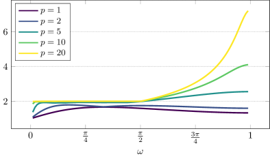
Figure 2. Dependence of $C_{\rm st,2}^{2}$ on the interior angle $\omega$ of the isosceles triangle $T=\mathrm{conv}\{(0,0),(1,0),(\cos(\omega),\sin(\omega))\}$

(Recall that the constants $C_{\rm st,1}$ and $C_{\rm st,2}$ are invariant under scaling.) This leads to our following conjecture in accordance with Figure 1 for any $p\in\mathbb{N}_{0}$.

Conjecture.

For triangles $T$ with maximal interior angle $\omega\leq\pi/2$, $C_{\rm st,2}\leq\sqrt{2}$.

3. The modified HHO method

This section introduces the HHO method and the discrete eigenvalue problem.

3.1. Triangulation

Let $\mathcal{T}$ be a regular triangulation of $\Omega$ into simplices in the sense of Ciarlet such that $\cup_{T\in\mathcal{T}}T=\overline{\Omega}$. Given a simplex $T\in\mathcal{T}$ of positive volume $|T|>0$, let $\mathcal{F}(T)$ denote the set of the $n+1$ hyperfaces of $T$, called sides of $T$. Define the set of all sides $\mathcal{F}=\cup_{T\in\mathcal{T}}\mathcal{F}(T)$ and the set of interior sides $\mathcal{F}(\Omega)=\mathcal{F}\setminus\{F\in\mathcal{F}:F\subset\partial\Omega\}$ in $\mathcal{T}$. For any interior side $F\in\mathcal{F}(\Omega)$, there exist exactly two simplices $T_{+},T_{-}\in\mathcal{T}$ such that $\partial T_{+}\cap\partial T_{-}=F$. The orientation of the outer normal unit $\nu_{F}=\nu_{T_{+}}|_{F}=-\nu_{T_{-}}|_{F}$ along $F$ is fixed and $\omega_{F}\coloneqq\mathrm{int}(T_{+}\cup T_{-})$ denotes the side patch of $F$. Let $[v]_{F}\coloneqq(v|_{T_{+}})|_{F}-(v|_{T_{-}})|_{F}\in L^{1}(F)$ denote the jump of $v\in L^{1}(\omega_{F})$ with $v\in W^{1,1}(T_{\pm})$ across $F$. For any boundary side $F\in\mathcal{F}(\partial\Omega)\coloneqq\mathcal{F}\setminus\mathcal{F}(\Omega)$, there exists a unique $T\in\mathcal{T}$ with $F\in\mathcal{F}(T)$. Then $\omega_{F}\coloneqq\mathrm{int}(T)$, $\nu_{F}\coloneqq\nu_{T}$ is the exterior unit vector of $F\in\mathcal{F}(T)$, and $[v]_{F}\coloneqq v|_{F}$. The triangulation $\mathcal{T}$ gives rise to the space $H^{1}(\mathcal{T})\coloneqq\{v\in L^{2}(\Omega):v|_{T}\in H^{1}(T)\}$ of piecewise Sobolev functions. The differential operators $\mathrm{div}_{\mathrm{pw}}$, $\nabla_{\mathrm{pw}}$, and $\Delta_{\mathrm{pw}}$ denote the piecewise applications of $\mathrm{div}$, $\nabla$, and $\Delta$ without explicit reference to the triangulation $\mathcal{T}$.

3.2. Discrete spaces

Let $P_{p}(\mathcal{T})$, $P_{p}(\mathcal{F})$, and $\mathrm{RT}^{\mathrm{pw}}_{p}(\mathcal{T})$ denote the space of piecewise functions with restrictions to $T\in\mathcal{T}$ or $F\in\mathcal{F}$ in $P_{p}(T)$, $P_{p}(F)$, and $\mathrm{RT}_{p}(T)$. The local mesh-sizes give rise to the piecewise constant function $h_{\mathcal{T}}\in P_{0}(\mathcal{T})$ with $h_{\mathcal{T}}|_{T}\equiv h_{T}=\mathrm{diam}(T)$ in $T\in\mathcal{T}$ and $h_{\max}\coloneqq\|h_{\mathcal{T}}\|_{L^{\infty}(\Omega)}$ abbreviates the maximal mesh-size of $\mathcal{T}$. The $L^{2}$ projections $\Pi_{p}:L^{1}(\Omega)\to P_{p}(\mathcal{T})$, $\Pi_{\mathcal{F}}^{p}:L^{1}(\cup\mathcal{F})\to P_{p}(\mathcal{F})$, and $\Pi_{\mathrm{RT}}:L^{1}(\Omega;\mathbb{R}^{n})\to\mathrm{RT}_{p}^{\mathrm{pw}}(\mathcal{T})$ onto $P_{p}(\mathcal{T})$, $P_{p}(\mathcal{F})$, and $\mathrm{RT}_{p}^{\mathrm{pw}}(\mathcal{T})$ are computed cell-wise. For vector-valued functions $\tau\in L^{1}(\Omega;\mathbb{R}^{n})$, the $L^{2}$ projection $\Pi_{p}$ onto $P_{p}(\mathcal{T};\mathbb{R}^{n})=P_{p}(\mathcal{T})^{n}$ applies componentwise. The Pythagoras theorem implies the stability of $L^{2}$ projections, for any $\tau\in L^{2}(\Omega;\mathbb{R}^{n})$ and $v\in L^{2}(\Omega)$,

(3.1) $$\|\Pi_{\mathrm{RT}}\tau\|_{L^{2}(\Omega)}^{2}\leq\|\tau\|_{L^{2}(\Omega)}\text{ and }\|\Pi_{p}v\|_{L^{2}(\Omega)}\leq\|v\|_{L^{2}(\Omega)}.$$

The Galerkin projection $Gf$ of $f\in H^{1}(\mathcal{T})$ is computed cell-wise by (1.12) with

(3.2) $$\|\nabla_{\mathrm{pw}}(1-G)f\|_{L^{2}(\Omega)}=\min_{p_{p+1}\in P_{p+1}(\mathcal{T})}\|\nabla_{\mathrm{pw}}(f-p_{p+1})\|_{L^{2}(\Omega)}.$$

The inclusion $\nabla_{\mathrm{pw}}P_{p+1}(\mathcal{T})\subset P_{p}(\mathcal{T};\mathbb{R}^{n})\subset\mathrm{RT}_{p}^{\mathrm{pw}}(\mathcal{T})$ leads, for any $f\in H^{1}(\mathcal{T})$, to

(3.3) $$\|(1-\Pi_{\mathrm{RT}})\nabla_{\mathrm{pw}}f\|_{L^{2}(\Omega)}\leq\|(1-\Pi_{p})\nabla_{\mathrm{pw}}f\|_{L^{2}(\Omega)}\leq\|\nabla_{\mathrm{pw}}(1-G)f\|_{L^{2}(\Omega)}.$$

3.3. HHO methodology

Let $V_{h}\coloneqq P_{p+1}(\mathcal{T})\times P_{p}(\mathcal{F}(\Omega))$ denote the ansatz space of the HHO method for $p\in\mathbb{N}_{0}$. The interior sides $\mathcal{F}(\Omega)$ give rise to the subspace $P_{p}(\mathcal{F}(\Omega))$ of all $(v_{F})_{F\in\mathcal{F}}\in P_{p}(\mathcal{F})$ with the convention $v_{F}\equiv 0$ on any boundary side $F\in\mathcal{F}(\partial\Omega)$ for homogenous boundary conditions. In other words, the notation $v_{h}\in V_{h}$ means $v_{h}=(v_{\mathcal{T}},v_{\mathcal{F}})=\big{(}(v_{T})_{T\in\mathcal{T}},(v_{F})_{F\in\mathcal{F}}\big{)}$ for some $v_{\mathcal{T}}\in P_{p+1}(\mathcal{T})$ and $v_{\mathcal{F}}\in P_{p}(\mathcal{F}(\Omega))$ with the identification $v_{T}=v_{\mathcal{T}}|_{T}\in P_{p+1}(T)$ and $v_{F}=v_{\mathcal{F}}|_{F}\in P_{p}(F)$. Given $v_{h}=(v_{\mathcal{T}},v_{\mathcal{F}})\in V_{h}$, the norm $\|v_{h}\|_{h}$ of $v_{h}$ in $V_{h}$ from [32, Eq. (28)] or [31, Eq. (41)] reads

(3.4) $$\|v_{h}\|_{h}^{2}\coloneqq\|\nabla_{\mathrm{pw}}v_{\mathcal{T}}\|^{2}_{L^{2}(T)}+\sum_{T\in\mathcal{T}}\sum_{F\in\mathcal{F}(T)}h_{F}^{-1}\|v_{F}-v_{T}\|^{2}_{L^{2}(F)}.$$

The interpolation $\mathrm{I}:V\to V_{h}$ maps $v\mapsto\mathrm{I}v\coloneqq(\Pi_{p+1}v,\Pi_{\mathcal{F}}^{p}v)\in V_{h}$.

Potential reconstruction. The potential reconstruction $\mathcal{R}v_{h}\in P_{p+1}(\mathcal{T})$ of $v_{h}=(v_{\mathcal{T}},v_{\mathcal{F}})\in V_{h}$ satisfies, for all discrete test functions $\varphi_{h}\in P_{p+1}(\mathcal{T})$, that

$$(\nabla_{\mathrm{pw}}\mathcal{R}v_{h},\nabla_{\mathrm{pw}}\varphi_{h})_{L^{2}(\Omega)}$$

(3.5) $$\qquad=-(v_{\mathcal{T}},\Delta_{\mathrm{pw}}\varphi_{h})_{L^{2}(\Omega)}+\sum_{F\in\mathcal{F}(\Omega)}\int_{F}v_{F}[\nabla_{\mathrm{pw}}\varphi_{h}\cdot\nu_{F}]_{F}\,\mathrm{d}s.$$

The bilinear form $(\nabla_{\mathrm{pw}}\bullet,\nabla_{\mathrm{pw}}\bullet)_{L^{2}(\Omega)}$ on the left-hand side of (3.5) defines a scalar product and the right-hand side of (3.5) is a linear functional in the quotient space $P_{p+1}(\mathcal{T})/P_{0}(\mathcal{T})$. The Riesz representation $\mathcal{R}v_{h}\in P_{p+1}(\mathcal{T})$ of this linear functional in $P_{p+1}(\mathcal{T})/P_{0}(\mathcal{T})$ is selected by

(3.6) $$\Pi_{0}\mathcal{R}v_{h}=\Pi_{0}v_{\mathcal{T}}.$$

The unique solution $\mathcal{R}v_{h}\in P_{p+1}(\mathcal{T})$ to (3.5)–(3.6) defines the potential reconstruction operator $\mathcal{R}:V_{h}\to P_{p+1}(\mathcal{T})$.

Gradient reconstruction. The gradient reconstruction $\mathcal{G}v_{h}\in\mathrm{RT}_{p}^{\mathrm{pw}}(\mathcal{T})$ of $v_{h}=(v_{\mathcal{T}},v_{\mathcal{F}})\in V_{h}$ satisfies, for all discrete test functions $\phi_{h}\in\mathrm{RT}_{p}^{\mathrm{pw}}(\mathcal{T})$, that

(3.7) $$(\mathcal{G}v_{h},\phi_{h})_{L^{2}(\Omega)}=-(v_{\mathcal{T}},\mathrm{div}_{\mathrm{pw}}\phi_{h})_{L^{2}(\Omega)}+\sum_{F\in\mathcal{F}(\Omega)}\int_{F}v_{F}[\phi_{h}\cdot\nu_{F}]_{F}\,\mathrm{d}s.$$

In other words, $\mathcal{G}v_{h}$ is the Riesz representation of the linear functional on the right-hand side of (3.7) in the Hilbert space $\mathrm{RT}_{p}^{\mathrm{pw}}(\mathcal{T})$ endowed with the $L^{2}$ scalar product. Since $\nabla_{\mathrm{pw}}P_{p+1}(\mathcal{T})\subset\mathrm{RT}_{p}^{\mathrm{pw}}(\mathcal{T})$, (3.7) implies the $L^{2}$ orthogonality $\mathcal{G}v_{h}-\mathcal{R}v_{h}\perp\nabla_{\mathrm{pw}}P_{p+1}(\mathcal{T})$. The following lemma recalls the commutativity of $\mathcal{G}$ and $\mathcal{R}$ [32, 31, 1, 33]. The Galerkin projection $G$ is defined in (1.12).

Lemma 3.1 (commutativity).

Any $v\in V$ satisfies $\mathcal{G}\mathrm{I}v=\Pi_{\mathrm{RT}}\nabla v$ and $\mathcal{R}\mathrm{I}v=Gv$.∎

3.4. Discrete eigenvalue problem

Given positive constants $0<\alpha<1$ and $0<\beta<\infty$, recall $a_{h}$ and $b_{h}$ from (1.6)–(1.7). Notice, for any $u_{h},v_{h}\in V_{h}$, that

(3.8) $$a_{h}(u_{h},v_{h})=((1-\alpha)\mathcal{G}u_{h}+\alpha\Pi_{p}\mathcal{G}u_{h},\mathcal{G}v_{h})_{L^{2}(\Omega)}+\beta(h_{\mathcal{T}}^{-2}Su_{h},Sv_{h})_{L^{2}(\Omega)}.$$

The discrete problem seeks a discrete eigenpair $(\lambda_{h},u_{h})\in\mathbb{R}_{+}\times V_{h}\setminus\{0\}$ such that

(3.9) $$a_{h}(u_{h},v_{h})=\lambda_{h}b_{h}(u_{h},v_{h})\text{ for all }v_{h}\in V_{h}.$$

Lemma 3.2 (discrete norm).

The bilinear form $a_{h}:V_{h}\times V_{h}\to\mathbb{R}$ is a scalar product in $V_{h}$. The induced norm $\|\bullet\|_{a,h}\coloneqq a_{h}(\bullet,\bullet)^{1/2}\approx\|\bullet\|_{h}$ is equivalent to the discrete norm $\|\bullet\|_{h}$ from (3.4).

Proof.

The equivalence $\|\bullet\|_{a,h}\approx\|v_{h}\|_{h}$ for all $v_{h}\in V_{h}$ is proven in [19, Lemma 3.5] for the stabilization $\beta(\nabla_{\mathrm{pw}}Su_{h},\nabla_{\mathrm{pw}}Sv_{h})_{L^{2}(\Omega)}$ instead of $\beta(h_{\mathcal{T}}^{-2}Su_{h},Sv_{h})_{L^{2}(\Omega)}$ in the definition (1.6) of $a_{h}$. Since the two stabilizations are locally equivalent, this leads to the assertion. ∎

The discrete eigenvalue problem (3.9) gives rise to the symmetric generalized algebraic eigenvalue problem

(3.10) $$\begin{pmatrix}A_{\mathcal{T}\mathcal{T}}&A_{\mathcal{T}\mathcal{F}}\\ A_{\mathcal{F}\mathcal{T}}&A_{\mathcal{F}\mathcal{F}}\end{pmatrix}\begin{pmatrix}x_{\mathcal{T}}\\ x_{\mathcal{F}}\end{pmatrix}=\lambda_{h}\begin{pmatrix}B_{\mathcal{T}\mathcal{T}}&0\\ 0&0\end{pmatrix}\begin{pmatrix}x_{\mathcal{T}}\\ x_{\mathcal{F}}\end{pmatrix}.$$

The application of the Schur complement as in [19, Section 3.3] leads to the algebraic eigenvalue problem $(A_{\mathcal{T}\mathcal{T}}-A_{\mathcal{T}\mathcal{F}}A_{\mathcal{F}\mathcal{F}}^{-1}A_{\mathcal{F}\mathcal{T}})x_{\mathcal{T}}=\lambda_{h}B_{\mathcal{T}\mathcal{T}}x_{\mathcal{T}}$. Hence, (3.10) provides $N\coloneqq\dim P_{p+1}(\mathcal{T})=|\mathcal{T}|\bigl{(}\begin{smallmatrix}p+1+n\\ n\end{smallmatrix}\bigr{)}$ positive discrete eigenvalues $0<\lambda_{h}(1)\leq\lambda_{h}(2)\leq\dots\leq\lambda_{h}(N)<\infty$; all other eigenvalues $\lambda_{h}(j)\coloneqq\infty$ for $j>N$ are infinity.

4. Lower eigenvalue bounds

This section establishes the sufficient conditions on the parameters $\alpha,\beta$ in (1.4) such that the HHO method from (3.9) provides direct GLB. Let $\lambda$ (resp. $\lambda_{h}$) denote the $j$-th continuous (resp. discrete) eigenvalue of (1.5) (resp. (3.9)) for fixed $j\in\mathbb{N}$. Recall $0<\alpha<1$, $0<\beta<\infty$, and the constant $\sigma_{2}$ from (2.1).

Theorem 4.1 (GLB).

If $\sigma_{2}^{2}\max\{\beta,h_{\max}^{2}\min\{\lambda_{h},\lambda\}\}\leq\alpha$, then $\lambda_{h}\leq\lambda$.

Remark 4.2 (GLB for $j>N$).

The number $j\in\mathbb{N}$ in the theorem can be larger than the dimension $N$. Then $\alpha<\sigma_{2}^{2}\lambda h_{\max}^{2}$ follows. In other words $\lambda(N+1)>\alpha\sigma_{2}^{-2}h_{\max}^{-2}$ is an a priori bound for the exact eigenvalue $\lambda(N+1)$ for free.

Proof of Theorem 4.1.

The proof applies the key arguments from [19, Theorem 4.1], but then reflects a different stabilization. This enables a different sufficient condition in the theorem with a more appropriate precise arrangement of the constants. (In fact, $G$ in (1.3)-(2.1) is replaced by $\Pi_{p+1}$ in [19], whence $C_{\mathrm{st,2}}$ in this paper is not larger than $C_{\mathrm{st},1}$ in [19] and $\kappa$ from [19] is bounded by $\sigma_{2}$ from (2.1).) Besides those differences, the first steps in the proof are very analogous and adopted for brevity.

Observe carefully that, in the beginning, $\sigma_{2}^{2}h_{\max}^{2}\min\{\lambda_{h},\lambda\}\leq\alpha$ does not immediately imply that $0<\lambda_{h}\leq\infty$ is finite.

Step 1: Reduction to $h_{\max}^{2}\sigma_{2}^{2}\lambda<1$. If $h_{\max}^{2}\sigma_{2}^{2}\lambda\geq 1$, then $h_{\max}^{2}\sigma_{2}^{2}\lambda_{h}\leq\alpha<1\leq h_{\max}^{2}\sigma_{2}^{2}\lambda$, whence $\lambda_{h}$ is finite and $\lambda_{h}\leq\lambda$. The remaining parts of this proof therefore assume $h_{\max}^{2}\sigma_{2}^{2}\lambda<1$.

Step 2: The first $j$ exact and pairwise orthonormal eigenfunctions $\phi_{1},\dots,\phi_{j}\in V$ of (1.5) satisfy that $\Pi_{p+1}\phi_{1},\dots,\Pi_{p+1}\phi_{j}\in P_{p+1}(\mathcal{T})$ are linear independent. The proof follows the lines of Step 2 in the proof of [19, Theorem 4.1] (with $\delta\coloneqq\sigma_{2}h_{\max}$).

Step 3: There exists $\phi\in\mathrm{span}\{\phi_{1},\dots,\phi_{j}\}$ with $\|\phi\|_{L^{2}(\Omega)}=1$, $\|\nabla\phi\|^{2}_{L^{2}(\Omega)}\leq\lambda$, and

(4.1) $$0<\lambda_{h}(1-\|(1-\Pi_{p+1})\phi\|_{L^{2}(\Omega)}^{2})\leq a_{h}(\mathrm{I}\phi,\mathrm{I}\phi).$$

The proof follows the lines of Step 3 in the proof of [19, Theorem 4.1] and considers the $\min$-$\max$ principle for the algebraic eigenvalue problem (3.10) with the $j$-dimensional subspace spanned by $\mathrm{I}\phi_{1},\dots,\mathrm{I}\phi_{j}\in V_{h}$. It is the linear independence of $\Pi_{p+1}\phi_{1},\dots,\Pi_{p+1}\phi_{j}\in P_{p+1}(\mathcal{T})$ that guarantees $j\leq N=\dim P_{p+1}(\mathcal{T})$ and that the algebraic eigenvalue problem (3.10) has at least $j$ finite eigenvalues; whence $\lambda_{h}=\lambda_{h}(j)<\infty$. The bound of $\lambda_{h}$ in the $\min$-$\max$ principle by some maximizer $v_{h}\coloneqq\mathrm{I}\phi$ of the Rayleigh quotient in $\mathrm{span}\{\mathrm{I}\phi_{1},\dots,\mathrm{I}\phi_{j}\}\subset V_{h}$ is rewritten as

$$\lambda_{h}b_{h}(\mathrm{I}\phi,\mathrm{I}\phi)\leq a_{h}(\mathrm{I}\phi,\mathrm{I}\phi)<\infty$$

for $\phi\in\mathrm{span}\{\phi_{1},\dots,\phi_{j}\}$ with $\|\phi\|_{L^{2}(\Omega)}=1$ and $\|\nabla\phi\|^{2}_{L^{2}(\Omega)}\leq\lambda$. It follows from Step 2 that $b_{h}(\mathrm{I}\phi,\mathrm{I}\phi)=\|\Pi_{p+1}\phi\|_{L^{2}(\Omega)}^{2}>0$ cannot vanish. This and the Pythagoras theorem $\|\Pi_{p+1}\phi\|_{L^{2}(\Omega)}^{2}=1-\|(1-\Pi_{p+1})\phi\|_{L^{2}(\Omega)}^{2}>0$ (recall $1=\|\phi\|^{2}_{L^{2}(\Omega)}$) conclude the proof of (4.1).

Step 4: First lower bound for $\lambda-\lambda_{h}$ under the assumption $\beta\sigma_{2}^{2}\leq\alpha$. The commutativity $\mathcal{G}\mathrm{I}\phi=\Pi_{\mathrm{RT}}\nabla\phi$ from Lemma 3.1.a and $(1-\alpha)\mathcal{G}u_{h}+\alpha\Pi_{p}\mathcal{G}u_{h}=(1-\alpha)(1-\Pi_{p})\mathcal{G}u_{h}+\Pi_{p}\mathcal{G}u_{h}$ for $u_{h}=\mathrm{I}\phi$ prove that $a_{h}(\mathrm{I}\phi,\mathrm{I}\phi)$ in (3.8) is equal to

(4.2) $$(1-\alpha)\|(1-\Pi_{p})\Pi_{\mathrm{RT}}\nabla\phi\|_{L^{2}(\Omega)}^{2}+\|\Pi_{p}\Pi_{\mathrm{RT}}\nabla\phi\|_{L^{2}(\Omega)}^{2}+\beta\|h_{\mathcal{T}}^{-1}S\mathrm{I}\phi\|_{L^{2}(\Omega)}^{2}.$$

The identity $\|(1-\Pi_{p})\Pi_{\mathrm{RT}}\nabla\phi\|_{L^{2}(\Omega)}=\|\Pi_{\mathrm{RT}}(1-\Pi_{p})\nabla\phi\|_{L^{2}(\Omega)}$ follows from the inclusion $P_{p}(\mathcal{T};\mathbb{R}^{n})\subset\mathrm{RT}_{p}^{\mathrm{pw}}(\mathcal{T})$ and $\Pi_{p}\Pi_{\mathrm{RT}}\nabla\phi=\Pi_{p}\nabla\phi=\Pi_{\mathrm{RT}}\Pi_{p}\phi$. This, (4.2), and $\|\Pi_{\mathrm{RT}}(1-\Pi_{p})\nabla\phi\|_{L^{2}(\Omega)}\leq\|(1-\Pi_{p})\nabla\phi\|_{L^{2}(\Omega)}$ from (3.1) lead to

(4.3) $$a_{h}(\mathrm{I}\phi,\mathrm{I}\phi)\leq\|\Pi_{p}\nabla\phi\|_{L^{2}(\Omega)}^{2}+(1-\alpha)\|(1-\Pi_{p})\nabla\phi\|_{L^{2}(\Omega)}^{2}+\beta\|h_{\mathcal{T}}^{-1}S\mathrm{I}\phi\|_{L^{2}(\Omega)}^{2}.$$

The Pythagoras theorem and $\|\nabla\phi\|_{L^{2}(\Omega)}^{2}\leq\lambda$ prove

(4.4) $$\|\Pi_{p}\nabla\phi\|_{L^{2}(\Omega)}^{2}\leq\lambda-\|(1-\Pi_{p})\nabla\phi\|^{2}_{L^{2}(\Omega)}.$$

Recall $S\mathrm{I}\phi=\Pi_{p+1}\phi-\mathcal{R}\mathrm{I}\phi=\Pi_{p+1}\phi-G\phi$ from Lemma 3.1.b. The piecewise mesh-size function $h_{\mathcal{T}}$ does not interfere with the projection $\Pi_{p+1}$ and so the Pythagoras theorem reads

(4.5) $$\|h_{\mathcal{T}}^{-1}S\mathrm{I}\phi\|_{L^{2}(\Omega)}^{2}=\|h_{\mathcal{T}}^{-1}(1-G)\phi\|_{L^{2}(\Omega)}^{2}-\|h_{\mathcal{T}}^{-1}(1-\Pi_{p+1})\phi\|_{L^{2}(\Omega)}^{2}.$$

The combination of (4.1) with (4.3)–(4.5) results in

$$-\lambda_{h}\|(1-\Pi_{p+1})\phi\|_{L^{2}(\Omega)}^{2}+\alpha\|(1-\Pi_{p})\nabla\phi\|_{L^{2}(\Omega)}^{2}$$

$$\qquad+\beta\|h_{\mathcal{T}}^{-1}(1-\Pi_{p+1})\phi\|_{L^{2}(\Omega)}^{2}-\beta\|h_{\mathcal{T}}^{-1}(1-G)\phi\|_{L^{2}(\Omega)}^{2}\leq\lambda-\lambda_{h}.$$

This, the stability estimate (2.1), and $h_{\max}^{-1}\leq h_{\mathcal{T}}^{-1}$ in $\Omega$ imply

$$(\beta/h_{\max}^{2}-\lambda_{h})\|(1-\Pi_{p+1})\phi\|_{L^{2}(\Omega)}^{2}$$

(4.6) $$\qquad\qquad+(\alpha-\beta\sigma_{2}^{2})\|(1-\Pi_{p})\nabla\phi\|_{L^{2}(\Omega)}^{2}\leq\lambda-\lambda_{h}.$$

Recall $\|(1-\Pi_{p+1})\phi\|_{L^{2}(\Omega)}^{2}\,\leq\|(1-G)\phi\|_{L^{2}(\Omega)}^{2}\leq\sigma_{2}^{2}h_{\max}^{2}\|(1-\Pi_{p})\nabla\phi\|_{L^{2}(\Omega)}^{2}$ from the best approximation property of $\Pi_{p+1}$ and (2.1) as well as $\alpha-\beta\sigma_{2}^{2}\geq 0$ from the assumptions. Consequently, the left-hand side of (4.6) is greater than or equal to $\|(1-\Pi_{p+1})\phi\|_{L^{2}(\Omega)}^{2}$ times

$$(\beta/h_{\max}^{2}-\lambda_{h}+(\alpha-\beta\sigma_{2}^{2})/(\sigma_{2}^{2}h_{\max}^{2}))=\alpha\sigma_{2}^{-2}h_{\max}^{-2}-\lambda_{h}.$$

In conclusion, $0\leq\|(1-\Pi_{p+1})\phi\|_{L^{2}(\Omega)}<1$ (from the end of Step 3) and

(4.7) $$(\alpha\sigma_{2}^{-2}h_{\max}^{-2}-\lambda_{h})\|(1-\Pi_{p+1})\phi\|_{L^{2}(\Omega)}^{2}\leq\lambda-\lambda_{h}.$$

Step 5: Finish of the proof. After the reduction to $h_{\max}^{2}\sigma_{2}^{2}\lambda<1$, the above Steps 2–4 of the proof have utilized $\beta\sigma_{2}^{2}\leq\alpha$, but they carefully avoided any assumption on $\lambda$ and $\lambda_{h}$, although it is supposed that $\sigma_{2}^{2}h_{\max}^{2}\min\{\lambda_{h},\lambda\}\leq\alpha$. In case that $\sigma_{2}^{2}h_{\max}^{2}\lambda_{h}\leq\alpha$, the assertion $0\leq\lambda-\lambda_{h}$ follows immediately from (4.7). In the remaining case $\sigma_{2}^{2}h_{\max}^{2}\lambda\leq\alpha$, the pre-factor in the left-hand side of (4.7) has the lower bound $\lambda-\lambda_{h}\leq\alpha\sigma_{2}^{-2}h_{\max}^{-2}-\lambda_{h}$. Therefore (4.7) implies

$$(\lambda-\lambda_{h})\|(1-\Pi_{p+1})\phi\|_{L^{2}(\Omega)}^{2}\leq\lambda-\lambda_{h}.$$

Recall that $0\leq\|(1-\Pi_{p+1})\phi\|_{L^{2}(\Omega)}<1$ from Step 4 to see that the last displayed estimate is impossible unless $0\leq\lambda-\lambda_{h}$. ∎

5. A priori error analysis

The Babuška-Osborn theory [4] for the spectral approximation of compact selfadjoint operators leads to a priori convergence rates for the approximation of $\lambda$ and of $u$ in the energy norm [12, 19]. This section establishes the quasi-best approximation estimate (1.9) for a simple eigenvalue $\lambda$, that eventually allows for the absorption of higher-order terms in the a posteriori error analysis of Section 6.

Throughout the remaining parts of this paper, suppose that $\beta\leq\alpha/\sigma_{2}^{2}$ with $\sigma_{2}$ from (2.1). Let $\lambda\coloneqq\lambda(j)$ be a simple eigenvalue of (1.5) with the corresponding eigenfunction $u\coloneqq u(j)\in V$. Let $(\lambda_{h},u_{h})\coloneqq(\lambda_{h}(j),u_{h}(j))$ denote the $j$-th discrete eigenpair of (3.9) with $u_{h}=(u_{\mathcal{T}},u_{\mathcal{F}})\in V_{h}$, $\|u\|_{L^{2}(\Omega)}=1=\|u_{\mathcal{T}}\|_{L^{2}(\Omega)}$, and $(u,u_{\mathcal{T}})_{L^{2}(\Omega)}\geq 0$. Recall that $0<s\leq 1$ denotes the minimum of the index of elliptic regularity and one.

Theorem 5.1 (a priori).

If $h_{\max}$ is sufficiently small, then (1.9) holds. The constant $C_{\ref{cnst:best-approximation}}$ exclusively depends on $p$, $n$, $\Omega$, and the shape regularity of $\mathcal{T}$.

The following lemmas precede the proof of Theorem 5.1. The first one recalls the enriching operator from [38] and adds the estimate (5.1). Recall the induced discrete norm $\|\bullet\|_{a,h}\coloneqq a_{h}(\bullet,\bullet)^{1/2}$ from Lemma 3.2.

Lemma 5.2 (enriching operator).

There exists a linear bounded operator $\mathrm{J}:V_{h}\to V$ that is a right-inverse of $\mathrm{I}$, i.e., $v_{h}=\mathrm{I}\mathrm{J}v_{h}=(\Pi_{p+1}\mathrm{J}v_{h},\Pi_{\mathcal{F}}^{p}\mathrm{J}v_{h})$ for all $v_{h}\in V_{h}$, and stable in the sense that $\|\nabla\mathrm{J}v_{h}\|_{L^{2}(\Omega)}\leq\|\mathrm{J}\|\|v_{h}\|_{a,h}$ with $\|\mathrm{J}\|\lesssim 1$. Any $v\in V$ satisfies

(5.1) $$\|\nabla(v-\mathrm{J}\mathrm{I}v)\|_{L^{2}(\Omega)}\leq C_{\ref{cnst:enrichment-operator}}\min_{v_{p+1}\in P_{p+1}(\mathcal{T})}\|\nabla_{\mathrm{pw}}(v-v_{p+1})\|_{L^{2}(\Omega)}.$$

The constants $\|\mathrm{J}\|$ and $C_{4}$ solely depend on $p$, $n$, and the shape regularity of $\mathcal{T}$.

Proof.

The construction of the enriching operator $\mathrm{J}:V_{h}\to V$ in spirit of [53] involves standard averaging and bubble-function techniques from [54] and is explained in [38, Section 4.3] for a related HHO method without the proof of (5.1). Notice that $\mathrm{J}$ from [38] (called stabilized bubble smoother $E_{\mathrm{H}}$ therein) only satisfies $\mathrm{J}v_{h}-v_{\mathcal{T}}\perp P_{p-1}(\mathcal{T})$ for any given $v_{h}=(v_{\mathcal{T}},v_{\mathcal{F}})\in V_{h}$. However, a straight-forward modification of [38, Eq. (4.16)] (in the notation of [38], $\mathcal{B}_{K}v_{\mathcal{M}}\in P_{p+1}(K)$ should be defined by equation (4.16) therein for all $q\in P_{p+1}(K)$) immediately provides a right-inverse $\mathrm{J}$ of $\mathrm{I}$. The arguments from [38, Propositions 4.5 and 4.7] apply and lead to the stability of $\mathrm{J}$ with respect to the equivalent discrete norm $\|\bullet\|_{h}\approx\|\bullet\|_{a,h}$ from Lemma 3.2.

It remains to prove (5.1) which is well-known for the Crouzeix-Raviart finite element method with an appropriate interpolation $\mathrm{I}$ and the conforming companion $\mathrm{J}$ from [21, Proposition 2.3] for $n=2$ and from [24, Section 5.8] for $n=3$. Given any $v_{h}\in V_{h}$, let $\mathcal{A}v_{h}\in S^{p+1}_{0}(\mathcal{T})\coloneqq P_{p+1}(\mathcal{T})\cap H^{1}_{0}(\Omega)$ denote the nodal average of $\mathcal{R}v_{h}$, cf. [38, Eq. (4.24)]. With [38, Eq. (4.18)] and with the above modification in [38, Eq. (4.16)], the bubble smoother $\mathcal{B}:L^{2}(\Omega)\times L^{2}(\bigcup\mathcal{F})\to H^{1}_{0}(\Omega)$ from [38, Proposition 4.6] satisfies, for $(v_{\mathcal{M}},v_{\Sigma})\in L^{2}(\Omega)\times L^{2}(\bigcup\mathcal{F})$, the stability estimate

(5.2) $$\|\nabla\mathcal{B}(v_{\mathcal{M}},v_{\Sigma})\|_{L^{2}(\Omega)}^{2}\lesssim\|h_{\mathcal{T}}^{-1}\Pi_{p+1}v_{\mathcal{M}}\|_{L^{2}(\Omega)}^{2}+\sum_{T\in\mathcal{T}}\sum_{F\in\mathcal{F}(T)}h_{F}^{-1}\|\Pi_{F}^{p}v_{\Sigma}\|_{L^{2}(F)}^{2}$$

with the $L^{2}$ projection $\Pi_{F}^{p}$ onto $P_{p}(F)$ for all faces $F\in\mathcal{F}$. A triangle inequality, the stability of $\Pi_{F}^{p}$ on a face $F$, and a discrete trace inequality show $\|\Pi_{F}^{p}(v_{F}-\mathcal{A}v_{h})\|_{L^{2}(F)}\leq\|\Pi_{F}^{p}(v_{F}-(\mathcal{R}v_{h})|_{T})\|_{L^{2}(F)}+h_{F}^{-1/2}\|\mathcal{R}v_{h}-\mathcal{A}v_{h}\|_{L^{2}(T)}$ for all $F\in\mathcal{F}(T)$ and $T\in\mathcal{T}$. This, a triangle inequality for $\mathrm{J}\coloneqq\mathcal{A}+\mathcal{B}(1-\mathcal{A})$, (5.2), and the second inequality on [38, p. 2180] result in

$$\|\nabla_{\mathrm{pw}}(\mathcal{R}v_{h}-\mathrm{J}v_{h})\|_{L^{2}(\Omega)}^{2}\lesssim\sum_{F\in\mathcal{F}}h_{F}^{-1}\|[\mathcal{R}v_{h}]_{F}\|_{L^{2}(\Omega)}^{2}$$

(5.3) $$\qquad+\|h_{\mathcal{T}}^{-1}(v_{\mathcal{T}}-\mathcal{R}v_{h})\|_{L^{2}(\Omega)}^{2}+\sum_{T\in\mathcal{T}}\sum_{F\in\mathcal{F}(T)}h_{F}^{-1}\|\Pi_{F}^{p}(v_{F}-(\mathcal{R}v_{h})|_{T})\|_{L^{2}(F)}^{2}.$$

Given $v\in V$, the stability of the $L^{2}$ projections $\Pi_{p+1}$ and $\Pi_{F}^{p}$ from (3.1) prove $\|\Pi_{p+1}(v-\mathcal{R}\mathrm{I}v)\|_{L^{2}(T)}\leq\|v-\mathcal{R}\mathrm{I}v\|_{L^{2}(T)}$ and $\|\Pi_{F}^{p}(v-\mathcal{R}(\mathrm{I}v)|_{T})\|_{L^{2}(F)}\leq\|v-(\mathcal{R}\mathrm{I}v)|_{T}\|_{L^{2}(F)}$ for all $T\in\mathcal{T}$ and $F\in\mathcal{F}(T)$. Given an interior side $F=T_{+}\cap T_{-}\in\mathcal{F}(\Omega)$ for $T_{\pm}\in\mathcal{T}$, the triangle inequality shows

$$\|[\mathcal{R}\mathrm{I}v]_{F}\|_{L^{2}(F)}=\|[\mathcal{R}\mathrm{I}v-v]_{F}\|_{L^{2}(F)}\leq\|(v-\mathcal{R}\mathrm{I}v)|_{T_{+}}\|_{L^{2}(F)}+\|(v-\mathcal{R}\mathrm{I}v)|_{T_{-}}\|_{L^{2}(F)}.$$

For boundary sides $F\in\mathcal{F}(\partial\Omega)$, it holds $\|[\mathcal{R}\mathrm{I}v]_{F}\|_{L^{2}(F)}=\|v-\mathcal{R}\mathrm{I}v\|_{L^{2}(F)}$. The choice $v_{h}\coloneqq\mathrm{I}v$ in (5.3), the aforementioned inequalities, the trace inequality, and the piecewise application of the Poincaré inequality imply $\|\nabla_{\mathrm{pw}}(\mathcal{R}\mathrm{I}v-\mathrm{J}\mathrm{I}v)\|_{L^{2}(\Omega)}\lesssim\|\nabla_{\mathrm{pw}}(v-\mathcal{R}\mathrm{I}v)\|_{L^{2}(\Omega)}$. This, the triangle inequality

$$\|\nabla(v-\mathrm{J}\mathrm{I}v)\|_{L^{2}(\Omega)}\leq\|\nabla_{\mathrm{pw}}(v-\mathcal{R}\mathrm{I}v)\|_{L^{2}(\Omega)}+\|\nabla_{\mathrm{pw}}(\mathcal{R}\mathrm{I}v-\mathrm{J}\mathrm{I}v)\|_{L^{2}(\Omega)},$$

and the $L^{2}$ orthogonality $\nabla_{\mathrm{pw}}(v-\mathcal{R}\mathrm{I}v)\perp\nabla_{\mathrm{pw}}P_{p+1}(\mathcal{T})$ conclude the proof of (5.1). ∎

The second lemma proves quasi-best approximation estimates for a source problem.

Lemma 5.3 (best-approximation).

Given $f\in L^{2}(\Omega)$, let $\widetilde{u}\in V$ solve $-\Delta\widetilde{u}=f$ in $\Omega$. The solution $\widetilde{u}_{h}=(\widetilde{u}_{\mathcal{T}},\widetilde{u}_{\mathcal{F}})\in V_{h}$ to

(5.4) $$a_{h}(\widetilde{u}_{h},v_{h})=(f,v_{\mathcal{T}})_{L^{2}(\Omega)}\quad\text{for all }v_{h}=(v_{\mathcal{T}},v_{\mathcal{F}})\in V_{h}$$

and the data oscillation $\mathrm{osc}(f,\mathcal{T})\coloneqq\|h_{\mathcal{T}}(1-\Pi_{p+1})f\|_{L^{2}(\Omega)}$ satisfy

(5.5) $$C_{\ref{cnst:best-approximation-source}}^{-1}\|\mathrm{I}\widetilde{u}-\widetilde{u}_{h}\|_{a,h}\leq\min_{v_{p+1}\in P_{p+1}(\mathcal{T})}\|\nabla_{\mathrm{pw}}(\widetilde{u}-v_{p+1})\|_{L^{2}(\Omega)}+\mathrm{osc}(f,\mathcal{T})$$

with the constant $C_{5}\coloneqq\max\{\|\mathrm{J}\|+(\alpha^{2}/(1-\alpha)+\beta C_{P}^{2})^{1/2},\|\mathrm{J}\|C_{P}\}$.

Proof.

Throughout this proof, abbreviate $\widetilde{e}_{h}\coloneqq\mathrm{I}\widetilde{u}-\widetilde{u}_{h}\in V_{h}$. Since $\Pi_{p+1}u-\widetilde{u}_{\mathcal{T}}=\Pi_{p+1}\mathrm{J}\widetilde{e}_{h}\in P_{p+1}(\mathcal{T})$ by Lemma 5.2, the discrete problem (5.4) shows

(5.6) $$a_{h}(\widetilde{u}_{h},\widetilde{e}_{h})=(f,\Pi_{p+1}\mathrm{J}\widetilde{e}_{h})_{L^{2}(\Omega)}.$$

The commutativity $\Pi_{\mathrm{RT}}\nabla v=\mathcal{G}\mathrm{I}v$ for $v\in V$ from Lemma 3.1 enters this proof in two ways. First, it verifies $\Pi_{p}\mathcal{G}\mathrm{I}\widetilde{u}=\Pi_{p}\nabla\widetilde{u}$ with $v\coloneqq\widetilde{u}$ so that (3.8) reads

(5.7) $$a_{h}(\mathrm{I}\widetilde{u},\widetilde{e}_{h}) =(\nabla\widetilde{u}-\alpha(1-\Pi_{p})\nabla\widetilde{u},\mathcal{G}\widetilde{e}_{h})_{L^{2}(\Omega)}+\beta(h_{\mathcal{T}}^{-2}S\mathrm{I}\widetilde{u},S\widetilde{e}_{h})_{L^{2}(\Omega)}.$$

Second, for $v\coloneqq\mathrm{J}\widetilde{e}_{h}$, the resulting $L^{2}$ orthogonality $\nabla\mathrm{J}\widetilde{e}_{h}-\mathcal{G}\widetilde{e}_{h}\perp\mathrm{RT}_{p}^{\mathrm{pw}}(\mathcal{T})$ to the piecewise Raviart-Thomas functions $\mathrm{RT}_{p}^{\mathrm{pw}}(\mathcal{T})$ provides

$$(\nabla\widetilde{u},\mathcal{G}\widetilde{e}_{h})_{L^{2}(\Omega)}=-((1-\Pi_{\mathrm{RT}})\nabla\widetilde{u},\nabla\mathrm{J}\widetilde{e}_{h})_{L^{2}(\Omega)}+(\nabla\widetilde{u},\nabla\mathrm{J}\widetilde{e}_{h})_{L^{2}(\Omega)}.$$

Since $\widetilde{u}\in V$ solves $-\Delta\widetilde{u}=f$ in $\Omega$, this and (5.6)–(5.7) verify

$$\|\widetilde{e}_{h}\|^{2}_{a,h} =(f,(1-\Pi_{p+1})\mathrm{J}\widetilde{e}_{h})_{L^{2}(\Omega)}-((1-\Pi_{\mathrm{RT}})\nabla\widetilde{u},\nabla\mathrm{J}\widetilde{e}_{h})_{L^{2}(\Omega)}$$

(5.8) $$\qquad-\alpha((1-\Pi_{p})\nabla\widetilde{u},\mathcal{G}\widetilde{e}_{h})_{L^{2}(\Omega)}+\beta(h_{\mathcal{T}}^{-2}S\mathrm{I}\widetilde{u},S\widetilde{e}_{h})_{L^{2}(\Omega)}.$$

The choice $\phi\coloneqq\widetilde{u}$ in (4.5) implies $\|h_{\mathcal{T}}^{-1}S\mathrm{I}\widetilde{u}\|_{L^{2}(\Omega)}\leq\|h_{\mathcal{T}}^{-1}(\widetilde{u}-G\widetilde{u})\|_{L^{2}(\Omega)}$ with the Galerkin projection $G$ from (1.12). Hence, the Poincaré inequality shows

(5.9) $$\|h_{\mathcal{T}}^{-1}S\mathrm{I}\widetilde{u}\|_{L^{2}(\Omega)}\leq C_{P}\|\nabla_{\mathrm{pw}}(\widetilde{u}-G\widetilde{u})\|_{L^{2}(\Omega)}.$$

A Cauchy and a piecewise application of the Poincaré inequality reveal

(5.10) $$(f,(1-\Pi_{p+1})\mathrm{J}\widetilde{e}_{h})_{L^{2}(\Omega)}\leq C_{P}\mathrm{osc}(f,\mathcal{T})\|\nabla\mathrm{J}\widetilde{e}_{h}\|_{L^{2}(\Omega)}.$$

The combination of (5.8)–(5.10) with a Cauchy inequality provides

$$\|\widetilde{e}_{h}\|_{a,h}^{2}\leq\big{(}C_{P}\mathrm{osc}(f,\mathcal{T})+\|(1-\Pi_{\mathrm{RT}})\nabla\widetilde{u}\|_{L^{2}(\Omega)}\big{)}\|\nabla\mathrm{J}\widetilde{e}_{h}\|_{L^{2}(\Omega)}$$

$$\quad+\alpha\|(1-\Pi_{p})\nabla\widetilde{u}\|_{L^{2}(\Omega)}\|\mathcal{G}\widetilde{e}_{h}\|_{L^{2}(\Omega)}+\beta C_{P}\|\nabla_{\mathrm{pw}}(\widetilde{u}-G\widetilde{u})\|_{L^{2}(\Omega)}\|h_{\mathcal{T}}^{-1}S\widetilde{e}_{h}\|_{L^{2}(\Omega)}.$$

This, (3.2)–(3.3), the stability $\|\nabla\mathrm{J}\widetilde{e}_{h}\|_{L^{2}(\Omega)}\leq\|\mathrm{J}\|\|\widetilde{e}_{h}\|_{a,h}$ from Lemma 5.2, a Cauchy inequality, and $(1-\alpha)\|\mathcal{G}\widetilde{e}_{h}\|_{L^{2}(\Omega)}^{2}+\beta\|h_{\mathcal{T}}^{-1}S\widetilde{e}_{h}\|_{L^{2}(\Omega)}^{2}\leq\|\widetilde{e}_{h}\|_{a,h}^{2}$ from (1.6) conclude the proof. ∎

The final lemma links (3.9) to (5.4). Recall the simple eigenpair $(\lambda,u)$ of (1.5) and the associated discrete eigenpair $(\lambda_{h},u_{h})$ of (3.9) with $u_{h}=(u_{\mathcal{T}},u_{\mathcal{F}})\in V_{h}$ and $(u,u_{\mathcal{T}})_{L^{2}(\Omega)}\geq 0$.

Lemma 5.4 (upper bound for $\|u-u_{\mathcal{T}}\|_{L^{2}(\Omega)}$).

If $h_{\max}$ is sufficiently small, then $\widetilde{u}_{h}=(\widetilde{u}_{\mathcal{T}},\widetilde{u}_{\mathcal{F}})\in V_{h}$ from Lemma 5.3 with $f\coloneqq\lambda u$ satisfies

$$\|u-u_{\mathcal{T}}\|_{L^{2}(\Omega)}\leq C_{\ref{cnst:spectral-gap}}\|u-\widetilde{u}_{\mathcal{T}}\|_{L^{2}(\Omega)}$$

with the constant $C_{6}\coloneqq\sqrt{2}(1+\max_{k\in\{1,\dots,N\}\setminus\{j\}}|\lambda/(\lambda_{h}(k)-\lambda)|)<\infty$.

Proof.

This follows as in [21, Lem. 2.4] with straight-forward modifications and is hence omitted. ∎

Proof of Theorem 5.1.

The proof of (1.9) is split into three steps.

Step 1 provides the $L^{2}$ error estimate

(5.11) $$\|u-u_{\mathcal{T}}\|_{L^{2}(\Omega)}\leq C_{\ref{cnst:best-approximation-step-1-final}}h_{\max}^{s}\min_{v_{p+1}\in P_{p+1}(\mathcal{T})}\|\nabla_{\mathrm{pw}}(u-v_{p+1})\|_{L^{2}(\Omega)}.$$

Recall $\widetilde{u}_{h}=(\widetilde{u}_{\mathcal{T}},\widetilde{u}_{\mathcal{F}})\in V_{h}$ from Lemma 5.3 with $f\coloneqq\lambda u$. Lemma 5.4, a triangle inequality, and (2.1) with $\|(1-\Pi_{p+1})u\|_{L^{2}(\Omega)}\leq\|(1-G)u\|_{L^{2}(\Omega)}$ lead to

(5.12) $$\|u-u_{\mathcal{T}}\|_{L^{2}(\Omega)}\leq C_{\ref{cnst:spectral-gap}}\sigma_{2}\|h_{\mathcal{T}}(1-\Pi_{p})\nabla u\|_{L^{2}(\Omega)}+C_{\ref{cnst:spectral-gap}}\|\Pi_{p+1}u-\widetilde{u}_{\mathcal{T}}\|_{L^{2}(\Omega)}.$$

Convergence rates for the error $\|\Pi_{p+1}u-\widetilde{u}_{\mathcal{T}}\|_{L^{2}(\Omega)}$ in HHO methods for a source problem are established in [32, 31, 38]. This proof follows [21, 38] and utilizes the operator $\mathrm{J}:V_{h}\to V$ from Lemma 5.2. Abbreviate $\widetilde{e}_{h}=(\widetilde{e}_{\mathcal{T}},\widetilde{e}_{\mathcal{F}})\coloneqq\mathrm{I}u-\widetilde{u}_{h}\in V_{h}$ and let $z\in V$ solve $-\Delta z=\widetilde{e}_{\mathcal{T}}$ in $\Omega$, i.e., $z\in V$ satisfies

(5.13) $$(\nabla z,\nabla v)_{L^{2}(\Omega)}=(\widetilde{e}_{\mathcal{T}},v)_{L^{2}(\Omega)}\quad\text{for all }v\in V.$$

Let $z_{C}\in S_{0}^{1}(\mathcal{T})\coloneqq P_{1}(\mathcal{T})\cap V$ denote the Scott-Zhang interpolation [50] of $z$ and observe that $(1-\Pi_{p})\nabla z_{C}\equiv 0$ vanishes. Lemma 3.1 implies $S\mathrm{I}z_{C}\equiv 0$ and therefore, the identity $a_{h}(\mathrm{I}z_{C},\widetilde{u}_{h})=(\nabla z_{C},\mathcal{G}\widetilde{u}_{h})$ follows from (3.8) with $\mathcal{G}\mathrm{I}z_{C}=\nabla z_{C}$. Lemma 3.1 and $\mathrm{I}\mathrm{J}=1$ verify $\Pi_{\mathrm{RT}}\nabla\mathrm{J}\mathrm{I}u=\mathcal{G}\mathrm{I}u=\Pi_{\mathrm{RT}}\nabla u$ and $\Pi_{\mathrm{RT}}\nabla\mathrm{J}\widetilde{u}_{h}=\mathcal{G}\widetilde{u}_{h}$. This, $\nabla z_{C}\in P_{0}(\mathcal{T};\mathbb{R}^{n})\subset\mathrm{RT}_{p}^{\mathrm{pw}}(\mathcal{T})$, and the symmetry of $a_{h}$ show

(5.14) $$(\nabla z_{C},\nabla\mathrm{J}\widetilde{e}_{h})_{L^{2}(\Omega)}=(\nabla z_{C},\nabla u-\mathcal{G}\widetilde{u}_{h})_{L^{2}(\Omega)}=a(u,z_{C})-a_{h}(\widetilde{u}_{h},\mathrm{I}z_{C})=0$$

with $a(u,z_{C})=\lambda(u,z_{C})_{L^{2}(\Omega)}=a_{h}(\widetilde{u}_{h},\mathrm{I}z_{C})$ from (1.5) and (5.4) in the last step. Hence, (5.13)–(5.14), a Cauchy inequality, and $\|\nabla\mathrm{J}\widetilde{e}_{h}\|_{L^{2}(\Omega)}\leq\|\mathrm{J}\|\|\widetilde{e}_{h}\|_{a,h}$ from Lemma 5.2 confirm

(5.15) $$(\widetilde{e}_{\mathcal{T}},\mathrm{J}\widetilde{e}_{h})_{L^{2}(\Omega)}=(\nabla(z-z_{C}),\nabla\mathrm{J}\widetilde{e}_{h})_{L^{2}(\Omega)}\leq\|\mathrm{J}\|\|\nabla(z-z_{C})\|_{L^{2}(\Omega)}\|\widetilde{e}_{h}\|_{a,h}.$$

The stability estimate (2.1) proves $\mathrm{osc}(\lambda u,\mathcal{T})\leq\lambda\sigma_{2}\|h_{\mathcal{T}}^{2}(1-\Pi_{p})\nabla u\|_{L^{2}(\Omega)}$. This, Lemma 5.3, and (3.3) provide

(5.16) $$\|\widetilde{e}_{h}\|_{a,h}\leq C_{\ref{cnst:best-approximation-source}}(1+\lambda\sigma_{2}h_{\max}^{2})\|\nabla_{\mathrm{pw}}(u-Gu)\|_{L^{2}(\Omega)}.$$

The elliptic regularity theory establishes $z\in V\cap H^{1+s}(\Omega)$ for $0<s\leq 1$ on the polyhedral Lipschitz domain $\Omega$ and the approximation property of the Scott-Zhang interpolation $z_{C}$ [50] provides the constants $C_{7},C_{8}$ depending exclusively on the domain $\Omega$ such that

$$C_{\ref{cnst:Scott-Zhang-approximation}}^{-1}h^{-s}_{\max}\|\nabla(z-z_{C})\|_{L^{2}(\Omega)}\leq\|z\|_{H^{1+s}(\Omega)}\leq C_{\ref{cnst:elliptic-regularity}}\|\widetilde{e}_{\mathcal{T}}\|_{L^{2}(\Omega)}.$$

Since $\Pi_{p+1}J\widetilde{e}_{h}=\widetilde{e}_{\mathcal{T}}=\Pi_{p+1}u-\widetilde{u}_{\mathcal{T}}$, the combination of (5.15)–(5.16) verifies

$$\|\Pi_{p+1}u-\widetilde{u}_{\mathcal{T}}\|_{L^{2}(\Omega)}^{2}=(\widetilde{e}_{\mathcal{T}},J\widetilde{e}_{h})_{L^{2}(\Omega)}\leq C_{\ref{cnst:best-approximation-step-1}}h_{\max}^{s}\|\nabla_{\mathrm{pw}}(u-Gu)\|_{L^{2}(\Omega)}\|\widetilde{e}_{\mathcal{T}}\|_{L^{2}(\Omega)}$$

with $C_{9}\coloneqq\|\mathrm{J}\|C_{\ref{cnst:best-approximation-source}}C_{\ref{cnst:Scott-Zhang-approximation}}C_{\ref{cnst:elliptic-regularity}}(1+\lambda\sigma_{2}h_{\max}^{2})$. This and (5.12) conclude the proof of (5.11) with $C_{10}\coloneqq C_{\ref{cnst:spectral-gap}}(\sigma_{2}h_{\rm max}^{1-s}+C_{\ref{cnst:best-approximation-step-1}})$ and Step 1.

Step 2 discusses the remaining term $|\lambda-\lambda_{h}|+\|\mathrm{I}u-u_{h}\|^{2}_{a,h}$ on the left-hand side of (1.9). Abbreviate $e_{h}\coloneqq\mathrm{I}u-u_{h}\in V_{h}$. Elementary algebra with the normalization $\|u\|_{L^{2}(\Omega)}=1=\|u_{\mathcal{T}}\|_{L^{2}(\Omega)}$ reveals $2\lambda=\lambda\|u-u_{\mathcal{T}}\|_{L^{2}(\Omega)}^{2}+2\lambda(u,u_{\mathcal{T}})_{L^{2}(\Omega)}$. This and $\|e_{h}\|_{a,h}^{2}-\lambda_{h}=\|\mathrm{I}u\|_{a,h}^{2}-2a_{h}(\mathrm{I}u,u_{h})$ result in

(5.17) $$\lambda-\lambda_{h}+\|e_{h}\|_{a,h}^{2}$$

$$\quad=\lambda\|u-u_{\mathcal{T}}\|^{2}_{L^{2}(\Omega)}+\|\mathrm{I}u\|_{a,h}^{2}-\lambda+2(\lambda(u,u_{\mathcal{T}})_{L^{2}(\Omega)}-a_{h}(\mathrm{I}u,u_{h})).$$

Step 2.1 bounds $\|\mathrm{I}u\|_{a,h}^{2}-\lambda$. The commutativity $\Pi_{\mathrm{RT}}\nabla u=\mathcal{G}\mathrm{I}u$ from Lemma 3.1 and (3.8) with $\Pi_{p}\Pi_{\mathrm{RT}}\nabla u=\Pi_{p}\nabla u$ show

$$\|\mathrm{I}u\|_{a,h}^{2}=(1-\alpha)(\Pi_{\mathrm{RT}}\nabla u,\nabla u)_{L^{2}(\Omega)}+\alpha(\Pi_{p}\nabla u,\nabla u)_{L^{2}(\Omega)}+\linebreak\beta\|h_{\mathcal{T}}^{-1}S\mathrm{I}u\|_{L^{2}(\Omega)}^{2}.$$

This and $\lambda=\|\nabla u\|_{L^{2}(\Omega)}^{2}$ prove

$$\|\mathrm{I}u\|_{a,h}^{2}-\lambda =\|\mathrm{I}u\|_{a,h}^{2}-\|\nabla u\|^{2}_{L^{2}(\Omega)}=-\alpha((1-\Pi_{p})\nabla u,\nabla u)_{L^{2}(\Omega)}$$

$$\quad-(1-\alpha)((1-\Pi_{\mathrm{RT}})\nabla u,\nabla u)_{L^{2}(\Omega)}+\beta\|h_{\mathcal{T}}^{-1}S\mathrm{I}u\|_{L^{2}(\Omega)}^{2}.$$

Thus, $0<\alpha<1$ and (5.9) with $\widetilde{u}$ replaced by $u$ imply

(5.18) $$\|\mathrm{I}u\|_{a,h}^{2}-\lambda\leq\beta\|h_{\mathcal{T}}^{-1}S\mathrm{I}u\|_{L^{2}(\Omega)}^{2}\leq\beta C_{P}^{2}\|\nabla_{\mathrm{pw}}(u-Gu)\|_{L^{2}(\Omega)}^{2}.$$

Step 2.2 controls $\lambda(u,u_{\mathcal{T}})_{L^{2}(\Omega)}-a_{h}(\mathrm{I}u,u_{h})$. The weak problem (1.5) and $\Pi_{p+1}\mathrm{J}u_{h}=u_{\mathcal{T}}$ reveal

(5.19) $$\lambda(u,u_{\mathcal{T}})_{L^{2}(\Omega)}=a(u,\mathrm{J}u_{h})-\lambda((1-\Pi_{p+1})u,\mathrm{J}u_{h})_{L^{2}(\Omega)}.$$

Lemma 3.1 provides $\Pi_{\mathrm{RT}}\nabla\mathrm{J}u_{h}=\mathcal{G}u_{h}$ and $\mathcal{G}\mathrm{I}u=\Pi_{\mathrm{RT}}\nabla u$. This and (3.8) lead to

$$a_{h}(\mathrm{I}u,u_{h})=((1-\alpha)\Pi_{\mathrm{RT}}\nabla u+\alpha\Pi_{p}\nabla u,\nabla\mathrm{J}u_{h})+\beta(h_{\mathcal{T}}^{-2}S\mathrm{I}u,Su_{h})_{L^{2}(\Omega)}.$$

This and (5.19) show

$$\lambda(u,u_{\mathcal{T}})_{L^{2}(\Omega)} -a_{h}(\mathrm{I}u,u_{h})=-\lambda((1-\Pi_{p+1})u,\mathrm{J}u_{h})_{L^{2}(\Omega)}-\beta(h_{\mathcal{T}}^{-2}S\mathrm{I}u,Su_{h})_{L^{2}(\Omega)}$$

$$+(1-\alpha)((1-\Pi_{\mathrm{RT}})\nabla u,\nabla\mathrm{J}u_{h})_{L^{2}(\Omega)}+\alpha((1-\Pi_{p})\nabla u,\nabla\mathrm{J}u_{h})_{L^{2}(\Omega)}.$$

Therefore, the Cauchy inequality and $P_{p}(\mathcal{T};\mathbb{R}^{n})\subset\mathrm{RT}_{p}^{\mathrm{pw}}(\mathcal{T};\mathbb{R}^{n})$ imply

$$\lambda(u, u_{\mathcal{T}})_{L^{2}(\Omega)}-a_{h}(\mathrm{I}u,u_{h})\leq\lambda\|(1-\Pi_{p+1})u\|_{L^{2}(\Omega)}\|(1-\Pi_{p+1})\mathrm{J}u_{h}\|_{L^{2}(\Omega)}$$

(5.20) $$+\|(1-\Pi_{p})\nabla u\|_{L^{2}(\Omega)}\|(1-\Pi_{p})\nabla\mathrm{J}u_{h}\|_{L^{2}(\Omega)}-\beta(h_{\mathcal{T}}^{-2}S\mathrm{I}u,Su_{h})_{L^{2}(\Omega)}.$$

In the following, we control the terms on the right-hand side of (5). The split $u_{h}=\mathrm{I}u-e_{h}$, $\|h_{\mathcal{T}}^{-1}S\mathrm{I}u\|_{L^{2}(\Omega)}\geq 0$, and a Cauchy inequality provide

$$-(h_{\mathcal{T}}^{-2}S\mathrm{I}u,Su_{h})_{L^{2}(\Omega)} \leq\|h_{\mathcal{T}}^{-1}S\mathrm{I}u\|_{L^{2}(\Omega)}\|h_{\mathcal{T}}^{-1}Se_{h}\|_{L^{2}(\Omega)}$$

(5.21) $$\leq C_{P}t/2\|\nabla_{\mathrm{pw}}(u-Gu)\|_{L^{2}(\Omega)}^{2}+C_{P}/(2t)\|h_{\mathcal{T}}^{-1}Se_{h}\|_{L^{2}(\Omega)}^{2}$$

from (5.9) with $\widetilde{u}$ replaced by $u$ and a Young inequality with arbitrary $t>0$ in the last step. Notice that $\Pi_{p}\nabla\mathrm{J}\mathrm{I}u=\mathcal{G}\mathrm{I}u=\Pi_{p}\nabla u$ by Lemma 3.1. Hence, a triangle inequality and $\|\nabla(u-\mathrm{J}\mathrm{I}u)\|_{L^{2}(\Omega)}\leq C_{\ref{cnst:enrichment-operator}}\|\nabla_{\mathrm{pw}}(u-Gu)\|_{L^{2}(\Omega)}$ from a combination of (5.1) with (3.2)–(3.3) verify

$$\|(1-\Pi_{p})\nabla\mathrm{J}\mathrm{I}u\|_{L^{2}(\Omega)} \leq\|(1-\Pi_{p})\nabla u\|_{L^{2}(\Omega)}+\|\nabla(u-\mathrm{J}\mathrm{I}u)\|_{L^{2}(\Omega)}$$

(5.22) $$\leq(1+C_{\ref{cnst:enrichment-operator}})\|\nabla_{\mathrm{pw}}(u-Gu)\|_{L^{2}(\Omega)}.$$

This, (2.1), a triangle inequality with the split $u_{h}=\mathrm{I}u-e_{h}$, and the stability $\|\nabla\mathrm{J}e_{h}\|_{L^{2}(\Omega)}\leq\|\mathrm{J}\|\|e_{h}\|_{a,h}$ from Lemma 5.2 provide

$$\sigma_{2}^{-1}h_{\rm max}^{-1} \|(1-\Pi_{p+1})\mathrm{J}u_{h}\|_{L^{2}(\Omega)}\leq\|(1-\Pi_{p})\nabla\mathrm{J}u_{h}\|_{L^{2}(\Omega)}$$

$$\leq\|(1-\Pi_{p})\nabla\mathrm{J}\mathrm{I}u\|_{L^{2}(\Omega)}+\|(1-\Pi_{p})\nabla\mathrm{J}e_{h}\|_{L^{2}(\Omega)}$$

(5.23) $$\leq(1+C_{\ref{cnst:enrichment-operator}})\|\nabla_{\mathrm{pw}}(u-Gu)\|_{L^{2}(\Omega)}+\|\mathrm{J}\|\|e_{h}\|_{a,h}.$$

The combination of (5)–(5) with (2.1) and a Young inequality with $t>0$ result in

$$\sigma_{2}^{-2}h_{\rm max}^{-2} \|(1-\Pi_{p+1})u\|_{L^{2}(\Omega)}\|(1-\Pi_{p+1})\mathrm{J}u_{h}\|_{L^{2}(\Omega)}$$

(5.24) $$\leq\|(1-\Pi_{p})\nabla u\|_{L^{2}(\Omega)}\|(1-\Pi_{p})\nabla\mathrm{J}u_{h}\|_{L^{2}(\Omega)}$$

$$\leq(1+C_{\ref{cnst:enrichment-operator}}+\|\mathrm{J}\|t/2)\|\nabla_{\mathrm{pw}}(u-Gu)\|_{L^{2}(\Omega)}^{2}+\|\mathrm{J}\|/(2t)\|e_{h}\|_{a,h}^{2}.$$

Then (5)–(5.21), (5)–(5.24) with the choice $t\coloneqq 2(1+\lambda\sigma_{2}^{2}h_{\rm max}^{2})\|\mathrm{J}\|+2C_{P}$, and $\beta\|h_{\mathcal{T}}^{-1}Se_{h}\|_{L^{2}(\Omega)}^{2}\leq\|e_{h}\|_{a,h}^{2}$ from (1.6) lead to

(5.25) $$\lambda(u,u_{\mathcal{T}})_{L^{2}(\Omega)}-a_{h}(\mathrm{I}u,u_{h})-\|e_{h}\|_{a,h}^{2}/4\leq C_{\ref{cnst:best-approximation-step-2-2}}\|\nabla_{\mathrm{pw}}(u-Gu)\|_{L^{2}(\Omega)}^{2}$$

with $C_{11}\coloneqq(1+\lambda\sigma_{2}^{2}h_{\rm max}^{2})(1+C_{\ref{cnst:enrichment-operator}}+\|\mathrm{J}\|t/2)+\beta C_{P}t/2$.

Step 3 finishes the proof. Theorem 4.1 guarantees $\lambda_{h}\leq\lambda$ for sufficiently small mesh-sizes $h_{\max}\leq(\alpha/(\lambda\sigma_{2}^{2}))^{1/2}$. This, the combination of (5.17)–(5.18) and (5.25) with the $L^{2}$ error estimate (5.11) from Step 1 results in

$$|\lambda-\lambda_{h}|+\|e_{h}\|_{a,h}^{2}/2\leq(\lambda C_{\ref{cnst:best-approximation-step-1-final}}^{{2}}h_{\rm max}^{2s}+\beta C_{P}^{2}+2C_{\ref{cnst:best-approximation-step-2-2}})\|\nabla_{\mathrm{pw}}(u-Gu)\|_{L^{2}(\Omega)}^{2}.$$

Thus, (5.11) and (3.2) conclude the proof of (1.9) with $C_{\ref{cnst:best-approximation}}\coloneqq 2(\lambda C_{\ref{cnst:best-approximation-step-1-final}}^{{2}}h_{\rm max}^{2s}+\beta C_{P}^{2}+2C_{\ref{cnst:best-approximation-step-2-2}})+C_{\ref{cnst:best-approximation-step-1-final}}^{2}$. ∎

Theorem 5.1 implies the following convergence rates and recovers [12, 19] for the eigenvalues and eigenfunctions error in the $H^{1}$ seminorm.

Corollary 5.5 (convergence).

If $u\in V\cap H^{1+t}(\Omega)$ for $s\leq t\leq p+1$, then

$$h_{\max}^{-s}\|u-u_{\mathcal{T}}\|_{L^{2}(\Omega)}+h_{\max}^{-t}\left(|\lambda-\lambda_{h}|+\|\mathrm{I}u-u_{h}\|_{a,h}^{2}\right)\lesssim h_{\max}^{t}\leavevmode\nobreak\ \text{as }h_{\max}\to 0.$$

Proof.

This follows immediately from Theorem 5.1, the stability (1.3), and standard approximation properties of piecewise polynomials [11, Lemma 4.3.8]. ∎

The techniques of this section also apply to the HHO method of [19] and lead to the optimal rate $s+t$ for the $L^{2}$ error towards a simple eigenvalue therein.

6. A posteriori error analysis

The two assumptions (A1)–(A2) below concern some $q\in H^{1}(\mathcal{T};\mathbb{R}^{n})$ and lead to a stabilization-free a posteriori error control of $\|\nabla u-q\|_{L^{2}(\Omega)}$ in two or three space dimensions. Let $\mathrm{RT}_{0}(\mathcal{T})\coloneqq\mathrm{RT}_{0}^{\mathrm{pw}}(\mathcal{T})\cap H(\mathrm{div})$ denote the lowest-order conforming Raviart-Thomas space, set $S^{m}_{0}(\mathcal{T})\coloneqq P_{m}(\mathcal{T})\cap H^{1}_{0}(\Omega)$ for $m\in\mathbb{N}$, and suppose

1. $(q,\nabla v_{C})_{L^{2}(\Omega)}=\lambda_{h}(u_{\mathcal{T}},v_{C})_{L^{2}(\Omega)}$ for all $v_{C}\in S_{0}^{1}(\mathcal{T})$,

2. $(q,q_{\mathrm{RT}})_{L^{2}(\Omega)}=0$ for all $q_{\mathrm{RT}}\in\mathrm{RT}_{0}(\mathcal{T})$ with $\mathrm{div}\,q_{\mathrm{RT}}=0$.

Theorem 6.1 (a posteriori).

Any $q\in H^{1}(\mathcal{T};\mathbb{R}^{n})$ with (A1)–(A2) and $\eta$ from (1.10) with $p_{h}$ replaced by $q$ satisfy

(6.1) $$C_{\ref{cnst:a-posteriori}}^{-1}\|\nabla u-q\|_{L^{2}(\Omega)}^{2}\leq\eta^{2}+\|\lambda u-\lambda_{h}u_{\mathcal{T}}\|^{2}_{L^{2}(\Omega)}.$$

The constant $C_{12}$ only depends on $p$, $n$, $\Omega$, and the shape regularity of $\mathcal{T}$.

Proof.

This is an extension of [8] to eigenvalue problems. For the convenience of the reader, the main arguments are briefly outlined below. Let $\psi\in V$ solve $-\Delta\psi=-\mathrm{div}\,q\in H^{-1}(\Omega)$ so that the Pythagoras theorem allows for the split

(6.2) $$\|\nabla u-q\|_{L^{2}(\Omega)}^{2}=\|\nabla(u-\psi)\|_{L^{2}(\Omega)}^{2}+\|\nabla\psi-q\|_{L^{2}(\Omega)}^{2}.$$

Upper bound for $\|\nabla(u-\psi)\|_{L^{2}(\Omega)}$. Abbreviate $\varrho\coloneqq u-\psi\in V$ and let $\varrho_{C}\in S^{1}_{0}(\mathcal{T})$ denote the Scott-Zhang interpolation of $\varrho$ [50]. Then (A1), $(\nabla\psi,\nabla\varrho)_{L^{2}(\Omega)}=(q,\nabla\varrho)_{L^{2}(\Omega)}$, and (1.5) lead to

$$\|\nabla\varrho\|^{2}_{L^{2}(\Omega)} =\lambda b(u,\varrho)-\lambda_{h}(u_{\mathcal{T}},\varrho_{C})_{L^{2}(\Omega)}-(q,\nabla(\varrho-\varrho_{C}))_{L^{2}(\Omega)}$$

(6.3) $$=(\lambda u-\lambda_{h}u_{\mathcal{T}},\varrho)_{L^{2}(\Omega)}+\lambda_{h}(u_{\mathcal{T}},\varrho-\varrho_{C})_{L^{2}(\Omega)}-(q,\nabla(\varrho-\varrho_{C}))_{L^{2}(\Omega)}.$$

The last two $L^{2}$ scalar products on the right-hand side of (6.3) arise in the explicit residual-based a posteriori error estimation of standard conforming FEM for the Poisson model problem, cf., e.g., [2, Section 2.2] or [37, Chapter 34], and are controlled by

$$\Big{(}\|h_{\mathcal{T}}(\mathrm{div}_{\mathrm{pw}}q+\lambda_{h}u_{\mathcal{T}})\|_{L^{2}(\Omega)}^{2}+\sum_{F\in\mathcal{F}(\Omega)}h_{F}\|[q\cdot\nu_{F}]_{F}\|_{L^{2}(F)}^{2}\Big{)}^{{1/2}}\|\nabla\varrho\|_{L^{2}(\Omega)}.$$

This, (6.3), a Cauchy inequality, and a Friedrichs inequality result in

(6.4) $$\|\nabla(u-\psi)\|_{L^{2}(\Omega)}^{2}\lesssim\eta^{2}+\|\lambda u-\lambda_{h}u_{\mathcal{T}}\|^{2}_{L^{2}(\Omega)}.$$

Upper bound for $\|\nabla\psi-q\|_{L^{2}(\Omega)}$. The function $\phi\coloneqq\nabla\psi-q\in L^{2}(\Omega;\mathbb{R}^{n})$ is divergence-free $\mathrm{div}\,\phi=0$ and orthogonal to the divergence-free Raviart-Thomas functions $q_{\mathrm{RT}}\in\mathrm{RT}_{0}(\mathcal{T})$ from (A2). The Helmholtz decomposition on a simply connected domain $\Omega$ immediately implies $\mathrm{Curl}\,\beta=\phi$ for some $\beta\in H^{1}(\Omega;\mathbb{R}^{2n-3})$, but in this paper, the domain $\Omega$ does not need to be simply connected. However, the extra condition (A2) ensures the existence of some orthogonal correction $\phi_{\mathrm{RT}}\in\mathrm{RT}_{0}(\mathcal{T})$ with $\mathrm{div}\,\phi_{\mathrm{RT}}=0$ such that the integrals $\int_{\Gamma_{j}}(\phi-\phi_{\mathrm{RT}})\cdot\nu\,\mathrm{d}s=0$ over the $J\in\mathbb{N}$ connectivity components $\Gamma_{j}$ for $j=1,...,J$ of $\partial\Omega$ vanish, cf. [8, Lemma 2] for further details. Thus classical theorems [40] imply the existence of $\beta\in H^{1}(\Omega;\mathbb{R}^{2n-3})$ such that $\mathrm{Curl}\,\beta=\phi-\phi_{\mathrm{RT}}$ and $\|\nabla\beta\|_{L^{2}(\Omega)}\lesssim\|\phi\|_{L^{2}(\Omega)}$. Since the Scott-Zhang interpolation $\beta_{C}\in S^{1}_{0}(\mathcal{T};\mathbb{R}^{2n-3})$ of $\beta$ satisfies $\mathrm{Curl}\,\beta_{C}\in\mathrm{RT}_{0}(\mathcal{T})$ and $\mathrm{div}\,\mathrm{Curl}\,\beta_{C}=0$, (A2) shows

$$\|\nabla\psi-q\|_{L^{2}(\Omega)}^{2}=(\phi,\mathrm{Curl}\,\beta+\phi_{\mathrm{RT}})_{L^{2}(\Omega)}=(\phi,\mathrm{Curl}(\beta-\beta_{C}))_{L^{2}(\Omega)}.$$

A piecewise integration by parts, the trace inequality, the approximation property of the Scott-Zhang interpolation [50], and the Cauchy inequality lead to

(6.5) $$\|\nabla\psi-q\|_{L^{2}(\Omega)}^{2}\lesssim\|h_{\mathcal{T}}\mathrm{curl}\,q\|_{L^{2}(\Omega)}^{2}+\sum_{F\in\mathcal{F}}h_{F}\|[q\times\nu_{F}]_{F}\|_{L^{2}(F)}^{2}.$$

The combination of (6.2) with (6.4)–(6.5) concludes the proof of (6.1). ∎

One key observation is that $q\coloneqq p_{h}\coloneqq\Pi_{p}\mathcal{G}u_{h}$ satisfies (A1)–(A2) as shown in the proof of Theorem 6.2 below. This leads to reliable a posteriori error control for $\|\nabla u-p_{h}\|_{L^{2}(\Omega)}$. Theorem 6.1 can also be applied to the HHO scheme of [12], where $q\coloneqq\nabla_{\mathrm{pw}}\mathcal{R}u_{h}$ satisfies (A1)–(A2) for $p\geq 1$. The lowest-order case $p=0$ therein can be treated separately as in [8].

Theorem 6.2 (reliability and efficiency).

For sufficiently small mesh-sizes $h_{\max}$, $p_{h}\coloneqq\Pi_{p}\mathcal{G}u_{h}\in P_{p}(\mathcal{T};\mathbb{R}^{n})$ and $\eta$ from (1.10) satisfy (1.11). The constants $C_{\mathrm{eff}}$ and $C_{\mathrm{rel}}$ exclusively depend on $p$, $n$, $\Omega$, and the shape regularity of $\mathcal{T}$.

Proof.

The first part of the proof verifies that $p_{h}=\Pi_{p}\mathcal{G}u_{h}$ satisfies (A1)–(A2).

Proof of (A1). Any $v_{C}\in S^{1}_{0}(\mathcal{T})$ satisfies $\nabla v_{C}=\mathcal{G}\mathrm{I}v_{C}\in P_{0}(\mathcal{T})$ and $v_{C}=\mathcal{R}\mathrm{I}v_{C}$. Thus $S\mathrm{I}v_{C}=0$ and so,

$$(p_{h},\nabla v_{C})_{L^{2}(\Omega)}=(\mathcal{G}u_{h},\nabla v_{C})_{L^{2}(\Omega)}=a_{h}(u_{h},\mathrm{I}v_{C})=\lambda_{h}(u_{\mathcal{T}},v_{C})_{L^{2}(\Omega)}.$$

Proof of (A2). Given $q_{\mathrm{RT}}\in\mathrm{RT}_{0}(\mathcal{T})\subset H(\mathrm{div},\Omega)$ with $\mathrm{div}\,q_{\mathrm{RT}}=0$, the normal jump $[q_{\mathrm{RT}}\cdot\nu_{F}]_{F}$ vanishes on any interior side $F\in\mathcal{F}(\Omega)$. Since divergence-free functions in $\mathrm{RT}_{0}(\mathcal{T})$ are piecewise constant, the definition of $\mathcal{G}$ from (3.7) shows $(p_{h},q_{\mathrm{RT}})_{L^{2}(\Omega)}=(\mathcal{G}u_{h},q_{\mathrm{RT}})_{L^{2}(\Omega)}=0$ and concludes the proof of (A2).

Proof of reliability. Since $q=p_{h}$ satisfies (A1)–(A2), Theorem 6.1 asserts

(6.6) $$C_{\ref{cnst:a-posteriori}}^{-1}\|\nabla u-p_{h}\|_{L^{2}(\Omega)}^{2}\leq\eta^{2}+\|\lambda u-\lambda_{h}u_{\mathcal{T}}\|^{2}_{L^{2}(\Omega)}.$$

The normalization $\|u\|_{L^{2}(\Omega)}=1=\|u_{\mathcal{T}}\|_{L^{2}(\Omega)}$, elementary algebra, and the combination of the a priori estimate (1.9) with (3.2) reveal

$$\|\lambda u-\lambda_{h}u_{\mathcal{T}}\|^{2}_{L^{2}(\Omega)} =(\lambda-\lambda_{h})^{2}+\lambda\lambda_{h}\|u-u_{\mathcal{T}}\|^{2}_{L^{2}(\Omega)}$$

(6.7) $$\leq C_{\ref{cnst:a-posteriori-absorption}}h_{\max}^{2s}\|\nabla_{\mathrm{pw}}(u-Gu)\|_{L^{2}(\Omega)}^{2}$$

with the elliptic regularity of $u\in V\cap H^{1+s}(\Omega)$ for the parameter $0<s\leq 1$ and $C_{13}\coloneqq\max\{|\lambda-\lambda_{h}|,\lambda\lambda_{h}\}C_{\ref{cnst:best-approximation}}$. The inequalities (1.3) and $p_{h}\in P_{p}(\mathcal{T};\mathbb{R}^{n})$ prove

(6.8) $$C_{\mathrm{st,2}}^{-1}\|\nabla_{\mathrm{pw}}(u-Gu)\|_{L^{2}(\Omega)}\leq\|(1-\Pi_{p})\nabla u\|_{L^{2}(\Omega)}\leq\|\nabla u-p_{h}\|_{L^{2}(\Omega)}.$$

For sufficiently small mesh-sizes $h_{\max}$, $C_{14}\coloneqq C_{\ref{cnst:a-posteriori}}C_{\ref{cnst:a-posteriori-absorption}}h_{\rm max}^{2s}C_{\rm st,2}^{2}<1$ and (6.6)–(6.8) lead to

(6.9) $$\|\nabla u-p_{h}\|_{L^{2}(\Omega)}^{2}\leq C_{\ref{cnst:a-posteriori}}(1-C_{\ref{cnst:a-posteriori-absorption-small-mesh-size}})^{-1}\eta^{2}.$$

Under the additional assumption $h_{\max}\leq(\alpha/(\lambda\sigma_{2}^{2}))^{1/2}$, the quasi-best approximation (1.9) and (6.8)–(6.9) conclude the proof of

(6.10) $$|\lambda-\lambda_{h}|+\|\mathrm{I}u-u_{h}\|_{a,h}^{2}+\|\nabla u-p_{h}\|_{L^{2}(\Omega)}^{2}\leq C_{\rm rel}\eta^{2}$$

with $C_{\rm rel}\coloneqq(1+C_{\ref{cnst:best-approximation}}C_{\rm st,2}^{2})C_{\ref{cnst:a-posteriori}}(1-C_{\ref{cnst:a-posteriori-absorption-small-mesh-size}})^{-1}$.

Proof of efficiency. The proof of $\eta^{2}\lesssim\|\nabla u-p_{h}\|_{L^{2}(\Omega)}^{2}$ utilizes bubble-function techniques from [54]. Similar arguments are employed in [29] for the Crouzeix-Raviart FEM and, e.g., in [2, 33, 8, 37] for the source problem. The efficiency $\sum_{F\in\mathcal{F}}h_{F}\|[p_{h}\times\nu_{F}]_{F}\|_{L^{2}(F)}^{2}\lesssim\|\nabla u-p_{h}\|^{2}_{L^{2}(\Omega)}$ follows from the arguments in the proof of [8, Lemma 7] for the Poisson model problem; hence further details are omitted. The focus is therefore on the proof of the efficiency of

$$\|h_{\mathcal{T}}\mathrm{curl}\,p_{h}\|_{L^{2}(\Omega)}^{2}+\|h_{\mathcal{T}}(\mathrm{div}\,p_{h}+\lambda_{h}u_{\mathcal{T}})\|^{2}_{L^{2}(\Omega)}+\sum_{F\in\mathcal{F}(\Omega)}h_{F}\|[p_{h}\cdot\nu_{F}]_{F}\|^{2}_{L^{2}(F)}.$$

Given $F\in\mathcal{F}(\Omega)$, let $b_{F}\in S^{n}(\mathcal{T})$ denote the face-bubble function with $0\leq b_{F}\leq 1$ in $\Omega$ and $\mathrm{supp}(b_{F})=\overline{\omega_{F}}$ [54, Section 3.1]. Define $\varrho\in S^{p+n}_{0}(\mathcal{T})$ such that $\varrho|_{F}=b_{F}[p_{h}\cdot\nu_{F}]_{F}\in P_{p+n}(F)$, $\mathrm{supp}(\varrho)=\overline{\omega_{F}}$, and $\varrho$ vanishes at all Lagrange points [11] in $\overline{\Omega}\setminus F$. Inverse estimates [54, Ineq. (3.2)] and an integration by parts prove, for any $F\in\mathcal{F}(\Omega)$, that

$$\|[p_{h}\cdot\nu_{F}]_{F}\|_{L^{2}(F)}^{2}\lesssim(\varrho,[p_{h}\cdot\nu_{F}]_{F})_{L^{2}(F)}=(\nabla\varrho,p_{h})_{L^{2}(\omega_{F})}+(\varrho,\mathrm{div}_{\mathrm{pw}}p_{h})_{L^{2}(\omega_{F})}.$$

This, $(\nabla u,\nabla\varrho)_{L^{2}(\omega_{F})}=\lambda(u,\varrho)_{L^{2}(\Omega)},$ and a Cauchy inequality imply

$$\|[p_{h}\cdot\nu_{F}]_{F}\|_{L^{2}(F)}^{2}\lesssim\|\nabla\varrho\|_{L^{2}(\omega_{F})}\|\nabla u-p_{h}\|_{L^{2}(\omega_{F})}$$

$$\qquad+\|\varrho\|_{L^{2}(\omega_{F})}\|\lambda u-\lambda_{h}u_{\mathcal{T}}\|_{L^{2}(\omega_{F})}+\|\varrho\|_{L^{2}(\omega_{F})}\|\mathrm{div}_{\mathrm{pw}}p_{h}+\lambda_{h}u_{\mathcal{T}}\|_{L^{2}(\omega_{F})}.$$

This, the inverse estimate $\|\nabla\varrho\|_{L^{2}(\omega_{F})}\lesssim h_{F}^{-1}\|\varrho\|_{L^{2}(\omega_{F})}$ [11, Lemma 4.5.3], and $\|\varrho\|_{L^{2}(\omega_{F})}^{2}\approx h_{F}\|\varrho\|_{L^{2}(F)}^{2}\leq h_{F}\|[p_{h}\cdot\nu_{F}]_{F}\|_{L^{2}(F)}^{2}$ [54, Ineq. (3.5)] show

(6.11) $$h_{F}\|[p_{h}\cdot\nu_{F}]_{F}\|^{2}_{L^{2}(F)}\lesssim\|\nabla u-p_{h}\|_{L^{2}(\omega_{F})}^{2}$$

$$\qquad+h_{F}^{2}\|\lambda u-\lambda_{h}u_{\mathcal{T}}\|_{L^{2}(\omega_{F})}^{2}+h_{F}^{2}\|\mathrm{div}_{\mathrm{pw}}p_{h}+\lambda_{h}u_{\mathcal{T}}\|_{L^{2}(\omega_{F})}^{2}.$$

Let $b_{T}\in P_{n+1}(T)\cap W^{1,\infty}_{0}(T)$ denote the volume-bubble function in $T\in\mathcal{T}$ with $0\leq b_{T}\leq 1$ and $b_{T}=0$ on $\partial T$ [54, Section 3.1]. Abbreviate $v_{p+1}\coloneqq\mathrm{div}\,p_{h}+\lambda_{h}u_{T}\in P_{p+1}(T)$ and define $\varphi\coloneqq b_{T}v_{p+1}\in S^{p+n+2}_{0}(T)\coloneqq P_{p+n+2}(T)\cap H^{1}_{0}(T)\subset V$. Inverse estimates [54, Ineq. (3.1)] and an integration by parts imply

(6.12) $$\|v_{p+1}\|_{L^{2}(T)}^{2}\lesssim(\varphi,v_{p+1})_{L^{2}(T)}=-(\nabla\varphi,p_{h})_{L^{2}(T)}+(\varphi,\lambda_{h}u_{T})_{L^{2}(T)}.$$

Since (the extension by zero of) $\varphi$ belongs to $V$, (1.5) provides $(\nabla\varphi,\nabla u)_{L^{2}(T)}=\lambda(u,\varphi)_{L^{2}(T)}$. This, (6.12), and a Cauchy inequality lead to

$$\|v_{p+1}\|_{L^{2}(T)}^{2}\lesssim\|\nabla\varphi\|_{L^{2}(T)}\|\nabla u-p_{h}\|_{L^{2}(T)}+\|\varphi\|_{L^{2}(T)}\|\lambda u-\lambda_{h}u_{T}\|_{L^{2}(T)}.$$

Hence $\|\varphi\|_{L^{2}(T)}=\|b_{T}v_{p+1}\|_{L^{2}(T)}\leq\|v_{p+1}\|_{L^{2}(T)}$ from $0\leq b_{T}\leq 1$ in $T$ and the inverse estimate $\|\nabla\varphi\|_{L^{2}(T)}\leq h_{T}^{-1}\|\varphi\|_{L^{2}(T)}$ [11, Lemma 4.5.3] reveal

(6.13) $$h_{T}^{2}\|\mathrm{div}\,p_{h}+\lambda_{h}u_{T}\|^{2}_{L^{2}(T)}\lesssim\|\nabla u-p_{h}\|_{L^{2}(T)}^{2}+h_{T}^{2}\|\lambda u-\lambda_{h}u_{T}\|_{L^{2}(T)}^{2}.$$

The local estimate $h_{T}\|\mathrm{curl}\,p_{h}\|_{L^{2}(T)}\lesssim\|\nabla u-p_{h}\|_{L^{2}(T)}$ follows from similar arguments as above and details are omitted. The combination of this with the local estimates (6.11) and (6.13) results in $\eta^{2}\lesssim\|\nabla u-p_{h}\|_{L^{2}(\Omega)}^{2}+\|h_{\mathcal{T}}(\lambda u-\lambda_{h}u_{\mathcal{T}})\|_{L^{2}(\Omega)}^{2}$. This and the control over $\|\lambda u-\lambda_{h}u_{\mathcal{T}}\|_{L^{2}(\Omega)}$ in (6.7)–(6.8) lead to the efficiency $\eta^{2}\lesssim\|\nabla u-p_{h}\|_{L^{2}(\Omega)}^{2}$. ∎

7. Numerical examples

The section presents three numerical benchmarks for the approximation of Dirichlet eigenvalues of the Laplacian on nonconvex domains $\Omega\subset\mathbb{R}^{2}$.

7.1. Parameter selection

For right-isosceles triangles, recall $C_{\mathrm{st,2}}\leq\sqrt{2}$ from Example 2.4 and $C_{P}=1/(\sqrt{2}\pi)$ from [44]. Throughout this section, let $\alpha=0.5$ and $\beta\coloneqq\alpha/\sigma_{2}^{2}=4.934802$ with $\sigma_{2}^{2}=C_{P}^{2}C_{\mathrm{st,2}}^{2}=1/\pi^{2}=0.101321$. The computable (a posteriori) condition $\sigma_{2}^{2}\max\{\beta,h_{\max}^{2}\lambda_{h}(j)\}\leq\alpha$ from Theorem 4.1 leads to $\mathrm{GLB}(j)\coloneqq\lambda_{h}(j)\leq\lambda(j)$. Since the parameters are chosen before-hand, the condition $h_{\max}^{2}\lambda_{h}\leq\alpha/\sigma_{2}^{2}=4.934802$ may not be satisfied on a coarse mesh with large $h_{\max}$ and $j$. In this case, $\mathrm{GLB}(j)\coloneqq 0$ (which is a guaranteed lower eigenvalue bound), so only GLB are displayed in this section.

7.2. Numerical realization

The algebraic eigenvalue problem (3.10) is realized with the iterative solver eigs from the MATLAB standard library in an extension of the data structures and short MATLAB programs in [3, 17]; the termination and round-off errors are expected to be very small and neglected for simplicity.

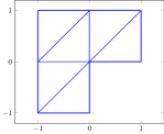
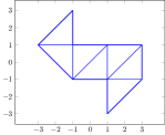
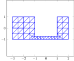
Figure 3. Initial triangulations of the L-shaped domain in Subsection 7.3, the isospectral drum in Subsection 7.4, and the dumbbell-slit domain in Subsection 7.5.

Figure 4. Polynomial degrees $p=0,\dots,4$ in the numerical benchmarks of Section 7.

The a posteriori estimate from Theorem 6.1 motivates the refinement indicator $\eta^{2}(T)$ from (1.10) with $\eta^{2}=\sum_{T\in\mathcal{T}}\eta^{2}(T)$. The standard adaptive algorithm [18, Algorithm 2.2] is modified in that, if $h_{\max}^{2}\lambda_{h}\leq\alpha/\sigma_{2}^{2}$ is not satisfied, the mesh is uniformly refined. It runs with the initial triangulations from Figure 3, the default bulk parameter $\theta=0.5$, and polynomial degrees $p$ displayed in Figure 4.

The uniform and adaptive mesh-refinements lead to convergence history plots of the eigenvalue error $\lambda(j)-\mathrm{GLB}(j)$ and the a posteriori estimate $\eta^{2}$ plotted against the number of degrees of freedom of $V_{h}$ (ndof) in log-log plots below; dashed (resp. solid) lines represent uniform (resp. adaptive) mesh-refinements.

7.3. L-shaped domain

The first example concerns the principle Dirichlet eigenvalue on the domain $\Omega\coloneqq(-1,1)^{2}\setminus([0,1)\times[0,-1))$ with a re-entering corner at $(0,0)$ and the reference value $\lambda(1)=9.6397238440219410$ from [9]. This leads to the suboptimal convergence rate $2/3$ for $\lambda(1)-\mathrm{GLB}(1)$ and $\eta^{2}$ (for all $p$) on uniform triangulations in Figure 5. The adaptive mesh-refining algorithm refines towards the origin as displayed in Figure 6 and recovers the optimal convergence rates $p+1$ for $\lambda(1)-\mathrm{GLB}(1)$ and $\eta^{2}$.

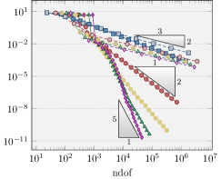
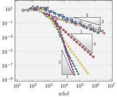
Figure 5. Convergence history plot of $\lambda(1)-\mathrm{GLB}(1)$ (left) and $\eta^{2}$ (right) for polynomial degrees $p$ from Figure 4 on uniform (dashed line) and adaptive (solid line) triangulations of the L-shaped domain in Subsection 7.3.

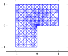
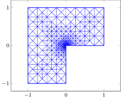
Figure 6. Adaptive triangulations of the L-shaped domain in Subsection 7.3 into 1034 triangles for $p=0$ (left) and into 1138 triangles for $p=3$ (right) for the approximation to $\lambda(1)$.

7.4. Isospectral domain

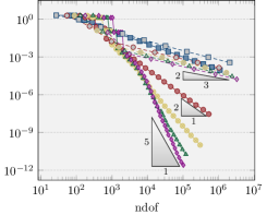
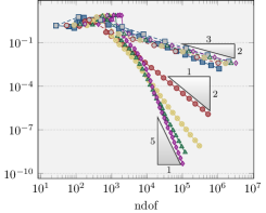
Figure 7. Convergence history plot of $\lambda(1)-\mathrm{GLB}(1)$ (left) and $\eta^{2}$ (right) for polynomial degrees $p$ from Figure 4 on uniform (dashed line) and adaptive (solid line) triangulations of the isospectral domain in Subsection 7.4.

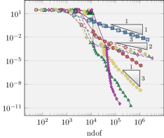
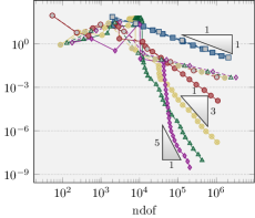
Figure 8. Convergence history plot of $\lambda(25)-\mathrm{GLB}(25)$ (left) and $\eta^{2}$ (right) for polynomial degrees $p$ from Figure 4 on uniform (dashed line) and adaptive (solid line) triangulations of the isospectral domain in Subsection 7.4.

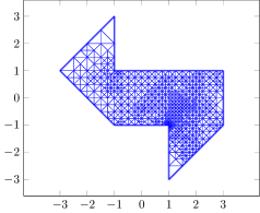
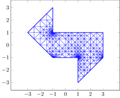
Figure 9. Adaptive triangulations of the isospectral domain in Subsection 7.4 into 1342 triangles for $p=0$ (left) and into 1311 triangles for $p=3$ (right) for the approximation to $\lambda(1)$.

The isospectral drums are pairs of non-isometric domains with identical spectrum of the Laplace operator. This subsection considers the domain $\Omega$ shown in Figure 3.b from [41]; the reference values $\lambda(1)=2.53794399980$ and $\lambda(25)=29.5697729132$ are from [9] and [34]. Figure 7 shows the suboptimal convergence rate $2/3$ for $\lambda(1)-\mathrm{GLB}(1)$ and $\eta^{2}$ for the approximation of the principle eigenvalue $\lambda(1)$ on uniformly refined triangulations. The adaptive mesh-refining algorithm refines towards four singular corners (for $p=3$) as depicted in Figure 9 and recovers the optimal convergence rates $p+1$ for $\lambda(1)-\mathrm{GLB}(1)$ and $\eta^{2}$. Figure 8 displays the empirical convergence rate $1$ for both $\lambda(25)-\mathrm{GLB}(25)$ and $\eta^{2}$ in case $p=0$, while it is the expected rate $2/3$ for $p\geq 1$ in the presence of a typical corner singularity in the eigenfunction. We conjecture that the singular contribution to the corresponding eigenfunction in this particular example has a very small coefficient and the reduced asymptotic convergence rate $2/3$ is therefore barely visible unless a very high accuracy is reached (e.g., absolute error in the eigenvalues much smaller than $5\times 10^{-4}$). The adaptive mesh-refining algorithm refines towards four re-entering corners and recovers the optimal convergence rates $p+1$ for $\lambda(25)-\mathrm{GLB}(25)$ and $\eta^{2}$. There are two reasons for the plateau observed in the convergence history plot of $\lambda(25)-\mathrm{GLB}(25)$ in Figure 8.a. First, a larger pre-asymptotic range is expected and observed for the approximation of larger eigenvalues. Second, the condition $h_{\max}^{2}\lambda_{h}\leq\alpha$ is not satisfied for the first triangulations, whence $\mathrm{GLB}$ is set to zero. An asymptotic behaviour is observed beyond 30,000 degrees of freedom for all displayed polynomial degrees $p=0,\dots,4$.

7.5. Dumbbell-slit domain

The final example approximates the principle Dirichlet eigenvalue $\lambda(1)$ on the domain $\Omega\coloneqq(-3,2)\times(-1,1)\setminus((-3,-2]\times\{0\}\cup[-1,1]\times[-3/4,1))$ displayed in Figure 3.c. This is a modification of the numerical example in [23, Section 4.2]. The reference value $\lambda(1)=8.367702430882$ stems from an adaptive computation with the polynomial degree $p=5$. The adaptive algorithm refines towards the reentrant corners at $(-1,-3/4)$ and $(-2,0)$ as displayed in Figure 10, while the triangles in the subdomain $(1,2)\times(-1,1)$ remain unchanged for $p\geq 1$. Hence, there may be no reduction of the maximal mesh-size $h_{\max}$. Figure 11 displays suboptimal convergence rate $0.5$ for the errors $\lambda(1)-\mathrm{GLB}(1)$ and $\eta^{2}$ for $p=0,\dots,4$. The adaptive mesh-refining recovers the optimal convergence rates $p+1$.

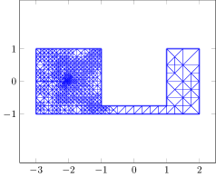
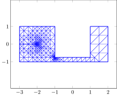
Figure 10. Adaptive triangulations of the dumbbell-slit domain in Subsection 7.5 into 1588 triangles for $p=0$ (left) and into 1505 triangles for $p=3$ (right) for the approximation to $\lambda(1)$.

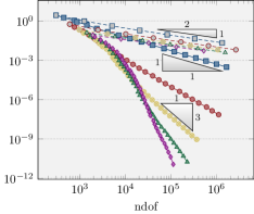
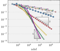
Figure 11. Convergence history plot of $\lambda(1)-\mathrm{GLB}(1)$ (left) and $\eta^{2}$ (right) for polynomial degrees $p$ from Figure 4 on uniform (dashed line) and adaptive (solid line) triangulations of the dumbbell-slit domain in Subsection 7.5.

7.6. Conclusions

The computer experiments provide empirical evidence for optimal convergence rates of the adaptive mesh-refining algorithm. The ad hoc choice $\alpha=1/2$ is robust in all computer experiments. For $\beta=\alpha/\sigma_{2}^{2}$, the computable condition $\sigma_{2}^{2}h_{\max}^{2}\lambda_{h}(j)\leq\alpha$ leads to confirmed lower eigenvalue bounds and holds on triangulations into right-isosceles triangles, whenever the maximal mesh-size $h_{\max}$ satisfies $\lambda_{h}h_{\max}^{2}\leq\alpha\pi^{2}$. In all displayed numerical benchmarks, $\lambda_{h}$ is a lower eigenvalue bound of $\lambda$ even for $\lambda_{h}h_{\max}^{2}>\alpha\pi^{2}$. The computed (but otherwise undisplayed) efficiency indices $7{\times}10^{-2}\leq I\coloneqq|\lambda-\lambda_{h}|\eta^{-2}\leq 4{\times}10^{-3}$ range in the numerical examples from $.07$ to $4{\times}10^{-3}$ for an asymptotic range $2{\times}10^{4}\leq\mathrm{ndof}\leq 10^{5}$; the quotient $I$ decreases for larger polynomial degree $p$. The overall numerical experience provides convincing evidence for the efficiency and reliability of the stabilization-free a posteriori error estimates of this paper. Higher polynomial degrees $p$ lead to significantly more accurate lower bounds and clearly outperform lowest-order discretizations.

Appendix: On $p$-robustness of constants
in refined $H^{1}$ stability estimates

This appendix provides details of the proof of Theorem 2.1 in the paper with focus on the constants $C_{\mathrm{st,1}},C_{\mathrm{st,2}}$ and their dependence on the polynomial degree $p\in\mathbb{N}_{0}$ in three space dimensions.

Overview

Let ${\left|\kern-1.07639pt\left|\kern-1.07639pt\left|\bullet\right|\kern-1.07639pt\right|\kern-1.07639pt\right|}\coloneqq\|\nabla\bullet\|_{L^{2}(T)}$ abbreviate the seminorm in the Sobolev space $H^{1}(T)\coloneqq H^{1}(\mathrm{int}(T))$ and let $\Pi_{p}$ denote the $L^{2}$ projection onto the space $P_{p}(T)$ of polynomials of total degree at most $p\in\mathbb{N}_{0}$ for a fixed tetrahedron $T\subset\mathbb{R}^{3}$. For any Sobolev function $f\in H^{1}(T)$, the Galerkin projection $Gf\in P_{p+1}(T)$ is the unique polynomial of degree at most $p+1$ with the prescribed integral mean $\Pi_{0}Gf=\Pi_{0}f$ and the orthogonality $\nabla(f-Gf)\perp\nabla P_{p+1}(T)$ in $L^{2}(T;\mathbb{R}^{3})$. The constants $C_{\mathrm{st,1}}$ and $C_{\mathrm{st,2}}$ are the best possible constants in the stability estimates

(1) $${\left|\kern-1.07639pt\left|\kern-1.07639pt\left|(1-\Pi_{p+1})f\right|\kern-1.07639pt\right|\kern-1.07639pt\right|} \leq C_{\textrm{st,1}}\|(1-\Pi_{p})\nabla f\|_{L^{2}(T)}\quad\text{for all }f\in H^{1}(T),$$

(2) $${\left|\kern-1.07639pt\left|\kern-1.07639pt\left|(1-G)f\right|\kern-1.07639pt\right|\kern-1.07639pt\right|} \leq C_{\textrm{st,2}}\|(1-\Pi_{p})\nabla f\|_{L^{2}(T)}\quad\text{for all }f\in H^{1}(T).$$

Theorem 2.1 asserts the following properties of $C_{\mathrm{st,1}}$ and $C_{\mathrm{st,2}}$.

1. There exist positive constants $1\leq C_{\mathrm{st,2}}\leq C_{\mathrm{st,1}}<\infty$ that satisfy (1)–(2). The constants $C_{\mathrm{st,1}}$ and $C_{\mathrm{st,2}}$ are independent of the diameter $h_{T}$ of $T$.

2. $C_{\mathrm{st,2}}$ is $p$ robust, i.e., $C_{\mathrm{st,2}}$ is uniformly bounded for all $p\in\mathbb{N}_{0}$.

3. $C_{\mathrm{st,1}}\approx\sqrt{p+1}$ is not $p$ robust.

The proof of $\|\Pi_{p+1}\|\leq C_{\rm st,1}\leq C_{\rm st,2}\|\Pi_{p+1}\|\lesssim\sqrt{p+1}$ is already explained in the paper and $\sqrt{p+1}\lesssim\|\Pi_{p+1}\|$ is established below in C.

A. Proof of existence

The two assumptions (H1)–(H2) from [25, Theorem 3.1] imply the existence of the constant $C_{\mathrm{st,1}}<\infty$ in [19, Theorem 2.3]. The $L^{2}$ orthogonality $\nabla(1-G)f\perp\nabla P_{p+1}(T)$ implies ${\left|\kern-1.07639pt\left|\kern-1.07639pt\left|(1-G)f\right|\kern-1.07639pt\right|\kern-1.07639pt\right|}\leq\|\nabla(1-\Pi_{p+1})f\|_{L^{2}(T)}$ for all $f\in H^{1}(T)$, whence $C_{\mathrm{st,1}}\leq C_{\mathrm{st,2}}<\infty$. The best approximation property of the $L^{2}$ projection $\Pi_{p}$ proves $\|(1-\Pi_{p})\nabla f\|_{L^{2}(T)}\leq{\left|\kern-1.07639pt\left|\kern-1.07639pt\left|(1-G)f\right|\kern-1.07639pt\right|\kern-1.07639pt\right|}$ and, therefore, $1\leq C_{\mathrm{st,1}}$. Notice that (A) holds in any space dimension.∎

B. Proof of $p$ robustness of $C_{\rm st,2}$

Let $\mathrm{N}_{p}(T)\coloneqq P_{p}(T;\mathbb{R}^{3})\oplus(P_{p}^{\mathrm{hom}}(T;\mathbb{R}^{3})\times x)=P_{p}(T;\mathbb{R}^{3})\oplus\{q\in P_{p+1}^{\mathrm{hom}}(T;\mathbb{R}^{3}):x\cdot q(x)=0\text{ for all }x\in T\}$ denote the first-kind Nédélec finite element space with the space $P_{p}^{\mathrm{hom}}(T;\mathbb{R}^{3})$ of homogenous polynomials of (total) degree $p$. Since $P_{p}(T;\mathbb{R}^{3})\subset\mathrm{N}_{p}(T)$, the $L^{2}$ projection $\Pi_{\mathrm{N}}$ onto $\mathrm{N}_{p}(T)$ satisfies $\|(1-\Pi_{\mathrm{N}})\nabla f\|_{L^{2}(T)}\leq\|(1-\Pi_{p})\nabla f\|_{L^{2}(T)}$ for all $f\in H^{1}(T)$. Hence, the existence of a constant $C(T)$ independent of $p$ and $\mathrm{diam}(T)$ such that

(3) $${\left|\kern-1.07639pt\left|\kern-1.07639pt\left|f-Gf\right|\kern-1.07639pt\right|\kern-1.07639pt\right|}\leq C(T)\|(1-\Pi_{\mathrm{N}})\nabla f\|_{L^{2}(T)}\quad\text{for all }f\in H^{1}(T)$$

implies (B). Given any $f\in H^{1}(T)$, abbreviate $q_{\mathrm{N}}\coloneqq\Pi_{\mathrm{N}}\nabla f\in\mathrm{N}_{p}(T)$ and observe $r_{\mathrm{RT}}\coloneqq\mathrm{curl}\,q_{\mathrm{N}}\in\mathrm{RT}_{p}(T)$ with $\mathrm{div}\,r_{\mathrm{RT}}=0$, e.g., from [36, Lemma 15.10], [10, Eq. (2.3.62)], or [48, Lemma 5.40]. It goes back to [28] to define a Bogovskiǐ-type integral operator as a pseudo-differential operator of order $-1$ of a Hörmander class $S^{-1}_{1,0}(\mathbb{R}^{n})$ that leads to right-inverses for differential operators. In particular, there exists a bounded linear operator $R^{\mathrm{curl}}:H^{-1}(T;\mathbb{R}^{3})\to L^{2}(T;\mathbb{R}^{3})$ such that $R_{\mathrm{N}}\coloneqq R^{\mathrm{curl}}r_{\mathrm{RT}}\in\mathrm{N}_{p}(T)$ satisfies $\mathrm{curl}\,R_{\mathrm{N}}=r_{\mathrm{RT}}$. Since $R_{\mathrm{N}}-q_{\mathrm{N}}\in\mathrm{N}_{p}(T)$ is curl-free by design, $R_{\mathrm{N}}-q_{\mathrm{N}}=\nabla\psi$ is the gradient of some function $\psi\in H^{1}(T)$ in the tetrahedron $T$. The structure of $\mathrm{N}_{p}(T)$ enforces $\psi\in P_{p+1}(T)$ (cf. [36, Lemma 15.10] and [48, Lemma 5.28] for the proof). Recall that $\nabla Gf$ is the best-approximation of $\nabla f$ in $\nabla P_{p+1}(T)$ and deduce (from $\nabla P_{p+1}(T)\subset P_{p}(T;\mathbb{R}^{3})\subset N_{p}(T)$) that it is also the best-approximation of $q_{\mathrm{N}}=\Pi_{\mathrm{N}}\nabla f$. Hence,

(4) $$\|\Pi_{\mathrm{N}}\nabla f-\nabla Gf\|_{L^{2}(T)}\leq\|q_{\mathrm{N}}\ +\nabla\psi\|_{L^{2}(T)}=\|R_{\mathrm{N}}\|_{L^{2}(T)}.$$

The operator norm $\|R^{\mathrm{curl}}\|$ of $R^{\mathrm{curl}}$ allows for $\|R_{\mathrm{N}}\|_{L^{2}(T)}\leq\|R^{\mathrm{curl}}\|{\left|\kern-1.07639pt\left|\kern-1.07639pt\left|r_{\mathrm{RT}}\right|\kern-1.07639pt\right|\kern-1.07639pt\right|}_{*}$ with the norm ${\left|\kern-1.07639pt\left|\kern-1.07639pt\left|\bullet\right|\kern-1.07639pt\right|\kern-1.07639pt\right|}_{*}$ in the dual space $H^{-1}(T;\mathbb{R}^{3})$ of $H^{1}_{0}(T;\mathbb{R}^{3})$ (endowed with the $H^{1}$ seminorm ${\left|\kern-1.07639pt\left|\kern-1.07639pt\left|\bullet\right|\kern-1.07639pt\right|\kern-1.07639pt\right|}$), i.e.,

$${\left|\kern-1.07639pt\left|\kern-1.07639pt\left|r_{\mathrm{RT}}\right|\kern-1.07639pt\right|\kern-1.07639pt\right|}_{*}=\sup_{v\in H^{1}_{0}(T;\mathbb{R}^{3})\setminus\{0\}}\int_{T}r_{\mathrm{RT}}\cdot v\,\mathrm{d}x/{\left|\kern-1.07639pt\left|\kern-1.07639pt\left|v\right|\kern-1.07639pt\right|\kern-1.07639pt\right|}.$$

Recall $r_{\mathrm{RT}}=\mathrm{curl}\,q_{\mathrm{N}}$. An integration by parts and $\mathrm{curl}\,\nabla f=0\in L^{2}(T)$ provide

$$\int_{T}r_{\mathrm{RT}}\cdot v\,\mathrm{d}x=\int_{T}\mathrm{curl}(q_{\mathrm{N}}-\nabla f)\cdot v\,\mathrm{d}x=\int_{T}(1-\Pi_{\mathrm{N}})\nabla f\cdot\mathrm{Curl}\,v\,\mathrm{d}x$$

for any $v\in H^{1}_{0}(T;\mathbb{R}^{3})$. This, a Cauchy inequality, and the estimate $\|\mathrm{Curl}\,v\|_{L^{2}(T)}\leq 2{\left|\kern-1.07639pt\left|\kern-1.07639pt\left|v\right|\kern-1.07639pt\right|\kern-1.07639pt\right|}/\sqrt{3}$ reveal ${\left|\kern-1.07639pt\left|\kern-1.07639pt\left|r_{\mathrm{RT}}\right|\kern-1.07639pt\right|\kern-1.07639pt\right|}_{*}\leq 2\|(1-\Pi_{\mathrm{N}})\nabla f\|_{L^{2}(T)}/\sqrt{3}$. Hence (4) implies

$$\|\Pi_{\mathrm{N}}\nabla f-\nabla Gf\|_{L^{2}(T)}\leq 2\|R^{\mathrm{curl}}\|\|(1-\Pi_{\mathrm{N}})\nabla f\|_{L^{2}(T)}/\sqrt{3}.$$

This and the Pythagoras theorem result in

$${\left|\kern-1.07639pt\left|\kern-1.07639pt\left|(1-G)f\right|\kern-1.07639pt\right|\kern-1.07639pt\right|}^{2} =\|(1-\Pi_{\mathrm{N}})\nabla f\|_{L^{2}(T)}^{2}+\|\Pi_{\mathrm{N}}\nabla f-\nabla Gf\|_{L^{2}(T)}^{2}$$

$$\leq(1+4\|R^{\mathrm{curl}}\|^{2}/3)\|(1-\Pi_{\mathrm{N}})\nabla f\|_{L^{2}(T)}^{2}.$$

This proves (3) with $C(T)\coloneqq\sqrt{1+4\|R^{\mathrm{curl}}\|^{2}/3}$ and, therefore, (B). More details on $\|R^{\mathrm{curl}}\|$ and further applications can be found in [28, Section 3], [42, Section 2], and [46, Lemma 6.4].

An alternative proof of (3) involves the main result of [26] and was kindly provided by A. Ern in private communications from 03/08/2022. For $v\coloneqq\nabla f\in H(\mathrm{curl},T)$ with $\mathrm{curl}\,v=0$, let $v_{h}^{*}$ (resp. $w_{h}^{*}$) denote the minimizer of $\|v-v_{h}\|_{L^{2}(\Omega)}$ among $v_{h}\in\mathcal{K}\coloneqq\{v_{h}\in N_{p}(T):\mathrm{curl}\,v=0\}$ (resp. $\|v-w_{h}\|_{L^{2}(\Omega)}$ among $w_{h}\in N_{p}(T)$). The $L^{2}$ orthogonality $w_{h}^{*}-v_{h}^{*}\perp\mathcal{K}$ from the Euler-Lagrange equations associated with these minimization problems implies that the difference $w_{h}^{*}-v_{h}^{*}$ minimizes the functional $\|z_{h}\|_{L^{2}(T)}$ among all $z_{h}\in w_{h}^{*}+\mathcal{K}$. Invoking the results of [28], it is known from [26, Theorem 2] that

$$\|w_{h}^{*}-v_{h}^{*}\|_{L^{2}(T)}=\inf_{\begin{subarray}{c}z_{h}\in\mathrm{N}_{p}(T)\\ \mathrm{curl}\,z_{h}=\mathrm{curl}\,w_{h}^{*}\end{subarray}}\|z_{h}\|_{L^{2}(T)}\leq\widetilde{C}(T)\inf_{\begin{subarray}{c}z\in H(\mathrm{curl},T)\\ \mathrm{curl}\,z=\mathrm{curl}\,w_{h}^{*}\end{subarray}}\|z\|_{L^{2}(T)}$$

with a $p$-robust constant $\widetilde{C}(T)>0$. Since $\mathrm{curl}(w_{h}^{*}-v)=\mathrm{curl}w_{h}^{*}$, we infer $\|w_{h}^{*}-v_{h}^{*}\|_{L^{2}(T)}\leq\widetilde{C}(T)\|v-w_{h}^{*}\|_{L^{2}(T)}$. This and a triangle inequality imply

$$\|v-v_{h}^{*}\|_{L^{2}(T)}\leq(1+\widetilde{C}(T))\|v-w_{h}^{*}\|_{L^{2}(T)}.$$

This is (3) with $C(T)\coloneqq 1+\widetilde{C}(T)$ because $w_{h}^{*}=\Pi_{\mathrm{N}}\nabla f$ by design and $v_{h}^{*}=\nabla Gf$ from $\mathcal{K}=\nabla P_{p+1}(T)$.∎

C. Lower growth $\sqrt{p+1}\lesssim\|\Pi_{p+1}\|$

While a compactness argument in [25, Theorem 3.1] leads to the existence of $C_{\mathrm{st,1}}$, the dependence of $C_{\mathrm{st,1}}$ on the polynomial degree $p$ remained obscured and only an upper bound for $p=0$ was given. The proof of Theorem 2.1 in the paper establishes

$$C_{\mathrm{st,1}}\approx\|\Pi_{p+1}\|\coloneqq\sup_{\phi\in H^{1}(T)\setminus\mathbb{R}}\frac{{\left|\kern-1.07639pt\left|\kern-1.07639pt\left|\Pi_{p+1}\phi\right|\kern-1.07639pt\right|\kern-1.07639pt\right|}}{{\left|\kern-1.07639pt\left|\kern-1.07639pt\left|\phi\right|\kern-1.07639pt\right|\kern-1.07639pt\right|}}.$$

An upper bound $\|\Pi_{p+1}\|\lesssim\sqrt{p+1}$ of the growth of the $H^{1}$ stability constant of the $L^{2}$ projection is known from [47, Sec. 5] and [55]. The remaining parts of this appendix therefore consider the reverse direction $\sqrt{p+1}\lesssim\|\Pi_{p+1}\|$ for a tetrahedron and depart with a motivating classical result in 1D. For simplicity, the following presentation applies an index shift and discusses $\|\Pi_{p}\|\approx\sqrt{p}$ for arbitrary $p\geq 1$.

Lower bound in 1D

In one space dimension, $\|\Pi_{p}\|\approx\sqrt{p}$ is established, e.g., in [16, Theorem 2.4] and [6, Remark 3.5]. Let $L_{k}$ for $k\in\mathbb{N}_{0}$ denote the Legendre polynomials in the reference interval $I\coloneqq(-1,1)$. Then $L_{k}$ satisfies, for all $k\in\mathbb{N}_{0}$,

(5) $$\widehat{L}_{k}(x) \coloneqq\int_{-1}^{x}L_{k}(t)\,\mathrm{d}t=\frac{L_{k+1}(x)-L_{k-1}(x)}{2k+1},$$

(6) $$\|L_{k}\|_{L^{2}(I)}^{2} =\frac{2}{2k+1}\leq\frac{1}{k},\quad\text{and}\quad\|\nabla L_{k}\|_{L^{2}(I)}^{2}=k(k+1)$$

with the convention $L_{-1}\equiv 0$ in $I$, cf., e.g., [7, Eqns (3.11), (3.12), (5.3)]. The pairwise $L^{2}$ orthogonality of $L_{k}$ and (5)–(6) lead to

$$\|\nabla\Pi_{p}\widehat{L}_{p}\|_{L^{2}(I)}^{2} =\frac{\|\nabla L_{p-1}\|_{L^{2}(I)}^{2}}{(2p+1)^{2}}=\frac{p(p-1)}{(2p+1)^{2}}\approx 1,$$

$$\|\nabla\widehat{L}_{p}\|_{L^{2}(I)}^{2} =\|L_{p}\|_{L^{2}(I)}^{2}=\frac{2}{2p+1}\approx p^{-1},$$

whence $\|\nabla\Pi_{p}\widehat{L}_{p}\|_{L^{2}(I)}\approx\sqrt{p}\|\nabla\widehat{L}_{p}\|_{L^{2}(I)}$ for all $p\geq 1$. This proves $\sqrt{p}\lesssim\|\Pi_{p}\|$ in 1D.

A similar result holds for the $L^{2}$ projection $\widetilde{\Pi}_{p}:L^{2}(D)\to Q_{p}(D)\cong P_{p}(I)^{n}$ onto the space of tensor-product polynomials on the $n$-cube $D\coloneqq I^{n}=(-1,+1)^{n}$ [16]. For simplicity and because the arguments carry over to triangles as well, the following proof considers simplices in $n=3$ dimensions only.

Proof of $\sqrt{p}\lesssim\|\Pi_{p}\|$ for $n=3$. Let $p\in\mathbb{N}$ be arbitrary and let $F:Q\to T$ denote the coordinate transformation

$$F(\eta_{1},\eta,\eta_{3})\coloneqq\left(\frac{(1+\eta_{1})(1-\eta_{2})(1-\eta_{3})}{4}-1,\frac{(1+\eta_{2})(1-\eta_{3})}{2}-1,\eta_{3}\right)$$

from the cube $Q\coloneqq(-1,1)^{3}$ onto the reference tetrahedron $T\coloneqq\mathrm{conv}\{(-1,-1,-1),\allowbreak(1,\allowbreak-1,\allowbreak-1),(-1,1,-1),(-1,-1,1)\}$ with the Jacobian $J_{F}$ and $\mathrm{det}J_{F}=(1-\eta_{2})(1-\eta_{3})^{2}/8$, see, e.g., [51] and [47, Section 3] for a derivation. An integration by substitution leads, for any $f\in L^{1}(Q)$, to

(7) $$\int_{T}f\circ F^{-1}\,\mathrm{d}x=\frac{1}{8}\int_{Q}(1-\eta_{2})(1-\eta_{3})^{2}f\,\mathrm{d}(\eta_{1},\eta_{2},\eta_{3}).$$

Define $\varphi(\eta_{2},\eta_{3})\coloneqq(1-\eta_{2})(1-\eta_{3})$, $U_{p}(\eta_{1},\eta_{2},\eta_{3})\coloneqq\varphi(\eta_{2},\eta_{3})^{p-1}\widehat{L}_{p}(\eta_{1})$, and $\widetilde{U}_{p}\coloneqq U_{p}\circ F^{-1}\in L^{2}(T)$ for $p\geq 1$. The chain rule $\nabla\widetilde{U}_{p}=J_{F}^{-\top}\nabla U_{p}\circ F^{-1}$ for the gradient and (5) provides $(\nabla\widetilde{U}_{p})\circ F=\varphi(\eta_{2},\eta_{3})^{p-2}M(\eta_{1},\eta_{2})G(\eta_{1})$ with

$$M(\eta_{1},\eta_{2})\coloneqq\begin{pmatrix}4&0&0\\ 2(1+\eta_{1})&2&0\\ 2(1+\eta_{1})&(1+\eta_{2})&(1-\eta_{2})\end{pmatrix} G(\eta_{1})\coloneqq\begin{pmatrix}L_{p}(\eta_{1})\\ (p-1)\widehat{L}_{p}(\eta_{1})\\ (p-1)\widehat{L}_{p}(\eta_{1})\end{pmatrix}.$$ and

A Cauchy inequality in $\mathbb{R}^{3}$ proves

$$|\nabla\widetilde{U}_{p}|^{2}\circ F =\varphi(\eta_{2},\eta_{3})^{2p-4}\sum^{3}_{j=1}\Big{(}\sum^{3}_{k=1}M_{jk}G_{k}\Big{)}^{2}\leq 3\varphi(\eta_{2},\eta_{3})^{2p-4}\sum^{3}_{k=1}\Big{(}\sum^{3}_{j=1}M_{jk}^{2}\Big{)}G_{k}^{2}.$$

This, the integration by substitution formula (7), $R_{p}\coloneqq\int_{-1}^{1}\int_{-1}^{1}(1-\eta_{2})^{2p-3}(1-\eta_{3})^{2p-2}\,\mathrm{d}(\eta_{2},\eta_{3})\in\mathbb{R}$, and $|\eta_{j}|\leq 1$ for $j=1,2,3$ and $(\eta_{1},\eta_{2},\eta_{3})\in Q$ show

$$\frac{1}{3}{\left|\kern-1.07639pt\left|\kern-1.07639pt\left|\widetilde{U}_{p}\right|\kern-1.07639pt\right|\kern-1.07639pt\right|}^{2}\leq \;\frac{1}{8}\int_{Q}(1-\eta_{2})(1-\eta_{3})^{2}c(\eta_{2},\eta_{3})^{2p-4}$$

$$\mkern-48.0mu\times\big{(}(16+8(1-\eta_{1})^{2})L_{p}(\eta_{1})^{2}+2(3+\eta_{2}^{2})(p-1)^{2}\widehat{L}_{p}(\eta_{1})^{2}\big{)}\,\mathrm{d}(\eta_{1},\eta_{2},\eta_{3})$$

$$\leq \;R_{p}\int_{-1}^{1}6L_{p}(\eta_{1})^{2}+(p-1)^{2}\widehat{L}_{p}(\eta_{1})^{2}\,\mathrm{d}\eta_{1}$$

(8) $$= \;R_{p}\big{(}6\|L_{p}\|_{L^{2}(I)}^{2}+\|(p-1)\widehat{L}_{p}\|_{L^{2}(I)}^{2}\big{)}.$$

The pairwise $L^{2}$ orthogonality of Legendre polynomials and (5)–(6) verify

$$p\|(p-1)\widehat{L}_{p}\|_{L^{2}(I)}^{2} =\frac{p(p-1)^{2}}{(2p+1)^{2}}\left(\|L_{p+1}\|_{L^{2}(I)}^{2}+\|L_{p-1}\|_{L^{2}(I)}^{2}\right)$$

$$=\frac{p(p-1)^{2}}{(2p+1)^{2}}\left(\frac{2}{2p+3}+\frac{2}{2p-1}\right)$$

$$=\frac{(p-1)^{2}p}{2(p-1/2)(p+1/2)(p+3/2)}\leq\frac{1}{2}$$

for $p\geq 1$. This, (6), and (8) provide the bound $2p{\left|\kern-1.07639pt\left|\kern-1.07639pt\left|\widetilde{U}_{p}\right|\kern-1.07639pt\right|\kern-1.07639pt\right|}^{2}\leq 39R_{p}$ for $p\geq 1$. It remains to control $\nabla\Pi_{p}\tilde{U}_{p}$ from below. Recall from [51] that the polynomials $\widetilde{\psi}_{j,k,\ell}\coloneqq\psi_{j,k,\ell}\circ F^{-1}\in P_{j+k+\ell}(T)$ for $j,k,\ell\in\mathbb{N}_{0}$ with

$$\psi_{j,k,\ell}(\eta_{1},\eta_{2},\eta_{3})\coloneqq L_{j}(\eta_{1})\left(1-\eta_{2}\right)^{j}P_{k}^{2j+1,0}(\eta_{2})\left(1-\eta_{3}\right)^{j+k}P_{\ell}^{2j+2k+2,0}(\eta_{3})$$

are $L^{2}(T)$ orthogonal and that $(\widetilde{\psi}_{j,k,\ell}\ |\ 0\leq j+k+\ell\leq p)$ forms a basis of $P_{p}(T)$. The pairwise orthogonality of the Legendre polynomials, (5), and (7) imply that

$$\left(\widetilde{U}_{p}+\frac{\widetilde{\psi}_{p-1,0,0}}{2p+1},\widetilde{\psi}_{j,k,\ell}\right)_{L^{2}(T)}=\left((1-\eta_{2})^{p}(1-\eta_{3})^{p+1}\frac{L_{p+1}(\eta_{1})}{2p+1},\psi_{j,k,\ell}\right)_{L^{2}(Q)}=0$$

vanishes for all $k,\ell\in\mathbb{N}$ and $j\leq p$. Consequently,

$$(2p+1)\Pi_{p}\widetilde{U}_{p}=-\widetilde{\psi}_{p-1,0,0}\in P_{p-1}(T).$$

This, the chain rule for partial derivatives, and (6)–(7) show

$$\left\|\frac{\partial}{\partial x}\Pi_{p}\widetilde{U}_{p}\right\|_{L^{2}(T)}^{2} =\frac{4^{2}R_{p}}{8(2p+1)^{2}}\int_{-1}^{1}\left(\frac{\mathrm{d}\phantom{A}}{\!\,\mathrm{d}\eta_{1}}L_{p-1}(\eta_{1})\right)^{2}\!\!\!\,\mathrm{d}\eta_{1}$$

(9) $$=\frac{2R_{p}}{(2p+1)^{2}}\|\nabla L_{p-1}\|_{L^{2}(I)}^{2}=\frac{2R_{p}}{(2p+1)^{2}}p(p-1).$$

The term $2p(p-1)(2p+1)^{-2}\geq 0$ is monotonically increasing in $p\geq 1$ and bounded from below by $4/25$ for $p\geq 2$. Thus, (9) and $2p{\left|\kern-1.07639pt\left|\kern-1.07639pt\left|\widetilde{U}_{p}\right|\kern-1.07639pt\right|\kern-1.07639pt\right|}^{2}\leq 39R_{p}$ provide

$$\frac{8}{975}p{\left|\kern-1.07639pt\left|\kern-1.07639pt\left|\widetilde{U}_{p}\right|\kern-1.07639pt\right|\kern-1.07639pt\right|}^{2}\leq\frac{4}{25}R_{p}\leq\left\|\frac{\partial}{\partial x}\Pi_{p}\widetilde{U}_{p}\right\|_{L^{2}(T)}^{2}\leq{\left|\kern-1.07639pt\left|\kern-1.07639pt\left|\Pi_{p}\widetilde{U}_{p}\right|\kern-1.07639pt\right|\kern-1.07639pt\right|}^{2}$$

for all $p\geq 2$, whence $\sqrt{p}\lesssim\|\Pi_{p}\|$ on the reference tetrahedron $T$. This and a scaling argument with an affine transformation concludes the proof for a general tetrahedron.∎

Acknowledgements

The authors gratefully thank Prof. Markus Melenk (Vienna University of Technology) for the discussion about the $H^{1}$ stability of the $L^{2}$ projection that eventually led to the proof of (C) and Prof. Alexandre Ern (CERMICS, ENPC) for his alternative proof of the $p$-robustness of $C_{\mathrm{st,2}}$ in (B).

References

- [1] M. Abbas, A. Ern and N. Pignet “Hybrid high-order methods for finite deformations of hyperelastic materials” In Comput. Mech. 62.4, 2018, pp. 909–928 DOI: 10.1007/s00466-018-1538-0
- [2] Mark Ainsworth and J. Tinsley Oden “A posteriori error estimation in finite element analysis” John Wiley & Sons, New York, 2000 DOI: 10.1002/9781118032824
- [3] Jochen Alberty, Carsten Carstensen and Stefan A. Funken “Remarks around 50 lines of Matlab: short finite element implementation” In Numer. Algorithms 20.2-3, 1999, pp. 117–137 DOI: 10.1023/A:1019155918070
- [4] I. Babuška and J. Osborn “Eigenvalue problems” In Handbook of numerical analysis, Vol. II North-Holland, Amsterdam, 1991, pp. 641–787
- [5] M. Bebendorf “A note on the Poincaré inequality for convex domains” In Z. Anal. Anwendungen 22.4, 2003, pp. 751–756 DOI: 10.4171/ZAA/1170
- [6] Christine Bernardi and Yvon Maday “Polynomial interpolation results in Sobolev spaces” In J. Comput. Appl. Math. 43.1-2, 1992, pp. 53–80 DOI: 10.1016/0377-0427(92)90259-Z
- [7] Christine Bernardi and Yvon Maday “Spectral methods” In Handbook of Numerical Analysis 5 Elsevier, 1997, pp. 209–485 DOI: 10.1016/S1570-8659(97)80003-8
- [8] Fleurianne Bertrand, Carsten Carstensen, Benedikt Gräßle and Ngoc Tien Tran “Stabilization-free HHO a posteriori error control” In Numer. Math. 154.3-4, 2023, pp. 369–408 DOI: 10.1007/s00211-023-01366-8
- [9] Timo Betcke and Lloyd N. Trefethen “Reviving the method of particular solutions” In SIAM Rev. 47.3, 2005, pp. 469–491 DOI: 10.1137/S0036144503437336
- [10] Daniele Boffi, Franco Brezzi and Michel Fortin “Mixed finite element methods and applications” Springer, Heidelberg, 2013 DOI: 10.1007/978-3-642-36519-5
- [11] Susanne C. Brenner and L. Ridgway Scott “The mathematical theory of finite element methods” Springer, New York, 2008 DOI: 10.1007/978-0-387-75934-0
- [12] Victor Calo, Matteo Cicuttin, Quanling Deng and Alexandre Ern “Spectral approximation of elliptic operators by the hybrid high-order method” In Math. Comp. 88.318, 2019, pp. 1559–1586 DOI: 10.1090/mcom/3405
- [13] Eric Cancès et al. “Guaranteed a posteriori bounds for eigenvalues and eigenvectors: multiplicities and clusters” In Math. Comp. 89.326, 2020, pp. 2563–2611 DOI: 10.1090/mcom/3549
- [14] Eric Cancès et al. “Guaranteed and robust a posteriori bounds for Laplace eigenvalues and eigenvectors: a unified framework” In Numer. Math. 140.4, 2018, pp. 1033–1079 DOI: 10.1007/s00211-018-0984-0
- [15] Eric Cancès et al. “Guaranteed and robust a posteriori bounds for Laplace eigenvalues and eigenvectors: conforming approximations” In SIAM J. Numer. Anal. 55.5, 2017, pp. 2228–2254 DOI: 10.1137/15M1038633
- [16] C. Canuto and A. Quarteroni “Approximation Results for Orthogonal Polynomials in Sobolev Spaces” In Math. Comp. 38.157, 1982, pp. 67–86 URL: http://www.jstor.org/stable/2007465
- [17] C. Carstensen and S. C. Brenner “Finite Element Methods” In Encyclopedia of Computational Mechanics Second Edition John WileySons, 2017, pp. 1–47
- [18] C. Carstensen, M. Feischl, M. Page and D. Praetorius “Axioms of adaptivity” In Comput. Math. Appl. 67.6, 2014, pp. 1195–1253 DOI: 10.1016/j.camwa.2013.12.003
- [19] Carsten Carstensen, Alexandre Ern and Sophie Puttkammer “Guaranteed lower bounds on eigenvalues of elliptic operators with a hybrid high-order method” In Numer. Math. 149.2, 2021, pp. 273–304 DOI: 10.1007/s00211-021-01228-1
- [20] Carsten Carstensen and Dietmar Gallistl “Guaranteed lower eigenvalue bounds for the biharmonic equation” In Numer. Math. 126.1, 2014, pp. 33–51 DOI: 10.1007/s00211-013-0559-z
- [21] Carsten Carstensen, Dietmar Gallistl and Mira Schedensack “Adaptive nonconforming Crouzeix-Raviart FEM for eigenvalue problems” In Math. Comp. 84.293, 2015, pp. 1061–1087 DOI: 10.1090/S0025-5718-2014-02894-9
- [22] Carsten Carstensen and Joscha Gedicke “Guaranteed lower bounds for eigenvalues” In Math. Comp. 83.290, 2014, pp. 2605–2629 DOI: 10.1090/S0025-5718-2014-02833-0
- [23] Carsten Carstensen and Sophie Puttkammer “Direct guaranteed lower eigenvalue bounds with optimal a priori convergence rates for the bi-Laplacian” In SIAM J. Numer. Anal. 61.2, 2023, pp. 812–836 DOI: 10.1137/21M139921X
- [24] Carsten Carstensen and Sophie Puttkammer “How to prove the discrete reliability for nonconforming finite element methods” In J. Comput. Math. 38.1, 2020, pp. 142–175 DOI: 10.4208/jcm.1908-m2018-0174
- [25] Carsten Carstensen, Qilong Zhai and Ran Zhang “A skeletal finite element method can compute lower eigenvalue bounds” In SIAM J. Numer. Anal. 58.1, 2020, pp. 109–124 DOI: 10.1137/18M1212276
- [26] Théophile Chaumont-Frelet, Alexandre Ern and Martin Vohralík “Polynomial-degree-robust -stability of discrete minimization in a tetrahedron” In C. R. Math. Acad. Sci. Paris 358.9-10, 2020, pp. 1101–1110 DOI: 10.5802/crmath.133
- [27] Bernardo Cockburn, Daniele A. Di Pietro and Alexandre Ern “Bridging the hybrid high-order and hybridizable dG methods” In ESAIM Math. Model. Numer. Anal. 50.3, 2016, pp. 635–650 DOI: 10.1051/m2an/2015051
- [28] Martin Costabel and Alan McIntosh “On Bogovskiĭ and regularized Poincaré integral operators for de Rham complexes on Lipschitz domains” In Math. Z. 265.2, 2010, pp. 297–320 DOI: 10.1007/s00209-009-0517-8
- [29] E. A. Dari, R. G. Durán and C. Padra “A posteriori error estimates for non-conforming approximation of eigenvalue problems” In Appl. Numer. Math. 62.5, 2012, pp. 580–591 DOI: 10.1016/j.apnum.2012.01.005
- [30] Daniele A. Di Pietro, Jérôme Droniou and Gianmarco Manzini “Discontinuous skeletal gradient discretisation methods on polytopal meshes” In J. Comput. Phys. 355, 2018, pp. 397–425 DOI: 10.1016/j.jcp.2017.11.018
- [31] Daniele A. Di Pietro and Alexandre Ern “A hybrid high-order locking-free method for linear elasticity on general meshes” In Comput. Methods Appl. Mech. Engrg. 283, 2015, pp. 1–21 DOI: 10.1016/j.cma.2014.09.009
- [32] Daniele A. Di Pietro, Alexandre Ern and Simon Lemaire “An arbitrary-order and compact-stencil discretization of diffusion on general meshes based on local reconstruction operators” In Comput. Methods Appl. Math. 14.4, 2014, pp. 461–472 DOI: 10.1515/cmam-2014-0018
- [33] Daniele Antonio Di Pietro and Roberta Tittarelli “An introduction to hybrid high-order methods” In Numerical methods for PDEs 15 Springer, Cham, 2018, pp. 75–128
- [34] Tobin A. Driscoll “Eigenmodes of isospectral drums” In SIAM Rev. 39.1, 1997, pp. 1–17 DOI: 10.1137/S0036144595285069
- [35] Ricardo G. Durán, Claudio Padra and Rodolfo Rodríguez “A posteriori error estimates for the finite element approximation of eigenvalue problems” In Math. Models Methods Appl. Sci. 13.8, 2003, pp. 1219–1229 DOI: 10.1142/S0218202503002878
- [36] Alexandre Ern and Jean-Luc Guermond “Finite elements I—Approximation and interpolation” Springer, 2021 DOI: 10.1007/978-3-030-56341-7
- [37] Alexandre Ern and Jean-Luc Guermond “Finite elements II—Galerkin approximation, elliptic and mixed PDEs” Springer, 2021 DOI: 10.1007/978-3-030-56923-5
- [38] Alexandre Ern and Pietro Zanotti “A quasi-optimal variant of the hybrid high-order method for elliptic partial differential equations with loads” In IMA J. Numer. Anal. 40.4, 2020, pp. 2163–2188 DOI: 10.1093/imanum/drz057
- [39] Dietmar Gallistl “Mixed methods and lower eigenvalue bounds” In Math. Comp. 92.342, 2023, pp. 1491–1509 DOI: 10.1090/mcom/3820
- [40] Vivette Girault and Pierre-Arnaud Raviart “Finite element methods for Navier-Stokes equations” Theory and algorithms Springer-Verlag, Berlin, 1986 DOI: 10.1007/978-3-642-61623-5
- [41] C. Gordon, D. Webb and S. Wolpert “Isospectral plane domains and surfaces via Riemannian orbifolds” In Invent. Math. 110.1, 1992, pp. 1–22 DOI: 10.1007/BF01231320
- [42] Ralf Hiptmair “Discrete Compactness for p-Version of Tetrahedral Edge Elements” In arXiv.org 0901.0761, 2009
- [43] Mats G. Larson “A posteriori and a priori error analysis for finite element approximations of self-adjoint elliptic eigenvalue problems” In SIAM J. Numer. Anal. 38.2, 2000, pp. 608–625 DOI: 10.1137/S0036142997320164
- [44] R. S. Laugesen and B. A. Siudeja “Minimizing Neumann fundamental tones of triangles: an optimal Poincaré inequality” In J. Differential Equations 249.1, 2010, pp. 118–135 DOI: 10.1016/j.jde.2010.02.020
- [45] Xuefeng Liu “A framework of verified eigenvalue bounds for self-adjoint differential operators” In Appl. Math. Comput. 267, 2015, pp. 341–355 DOI: 10.1016/j.amc.2015.03.048
- [46] J. M. Melenk and C. Rojik “On commuting -version projection-based interpolation on tetrahedra” In Math. Comp. 89.321, 2020, pp. 45–87 DOI: 10.1090/mcom/3454
- [47] Jens Markus Melenk and Tobias Wurzer “On the stability of the boundary trace of the polynomial L2-projection on triangles and tetrahedra (extended version)” In arxiv.org 1302.7189, 2013 DOI: 10.48550/ARXIV.1302.7189
- [48] Peter Monk “Finite element methods for Maxwell’s equations” Oxford University Press, New York, 2003 DOI: 10.1093/acprof:oso/9780198508885.001.0001
- [49] L. E. Payne and H. F. Weinberger “An optimal Poincaré inequality for convex domains” In Arch. Rational Mech. Anal. 5, 1960, pp. 286–292 (1960) DOI: 10.1007/BF00252910
- [50] L. Ridgway Scott and Shangyou Zhang “Finite element interpolation of nonsmooth functions satisfying boundary conditions” In Math. Comp. 54.190, 1990, pp. 483–493 DOI: 10.2307/2008497
- [51] Spencer J. Sherwin and George Em Karniadakis “A new triangular and tetrahedral basis for high-order (hp) finite element methods” In International Journal for Numerical Methods in Engineering 38.22, 1995, pp. 3775–3802 DOI: https://doi.org/10.1002/nme.1620382204
- [52] Daniel B. Szyld “The many proofs of an identity on the norm of oblique projections” In Numer Algor 42.3-4, 2006, pp. 309–323 DOI: 10.1007/s11075-006-9046-2
- [53] Andreas Veeser and Pietro Zanotti “Quasi-optimal nonconforming methods for symmetric elliptic problems. II—Overconsistency and classical nonconforming elements” In SIAM J. Numer. Anal. 57.1, 2019, pp. 266–292 DOI: 10.1137/17M1151651
- [54] R. Verfürth “A Review of A Posteriori Error Estimation and Adaptive Mesh-Refinement Techniques” John Wiley & Sons., Chichester, 1996
- [55] T Wurzer “Stability of the trace of the polynomial L2-projection on triangles” In Technical Report 36, Institute for Analysis and Scientific Computing, Vienna, 2010