Miura transformations and large-time behaviors of the Hirota-Satsuma equation

Abstract.

The good Boussinesq equation has several modified versions such as the modified Boussinesq equation, Mikhailov-Lenells equation and Hirota-Satsuma equation. This work builds the full relations among these equations by Miura transformation and invertible linear transformations and draws a pyramid diagram to demonstrate such relations. The direct and inverse spectral analysis shows that the solution of Riemann-Hilbert problem for Hirota-Satsuma equation has simple pole at origin, the solution of Riemann-Hilbert problem for the good Boussinesq equation has double pole at origin, while the solution of Riemann-Hilbert problem for the modified Boussinesq equation and Mikhailov-Lenells equation doesn’t have singularity at origin. Further, the large-time asymptotic behaviors of the Hirota-Satsuma equation with Schwartz class initial value is studied by Deift-Zhou nonlinear steepest descent analysis. In such initial condition, the asymptotic expressions of the Hirota-Satsuma equation and good Boussinesq equation away from the origin are proposed and it is displayed that the leading term of asymptotic formulas match well with direct numerical simulations.

1. Introduction

Starting from the Bäcklund transformation of the Boussinesq equation [1, 2, 3, 4], Hirota and Satsuma [5] initially proposed the Hirota-Satsuma equation

$$u_{tt}+\frac{1}{3}(u_{xxx}-\frac{2}{3}u^{2}u_{x}-2u_{x}\partial_{x}^{-1}u_{t})_{x}=0,$$ (1.1)

where $\partial_{x}^{-1}$ is the inverse operator of operator $\partial=\partial/\partial x$, which is defined as $(\partial_{x}^{-1}g)(x)=\int_{-\infty}^{x}g(y)dy$ with $\partial\partial_{x}^{-1}=\partial_{x}^{-1}\partial=1$. Introducing special constrain to $u_{t}$ in [6, 7], the Hirota-Satsuma equation (1.1) is equivalent to

$$u_{t}=-u_{xx}+\frac{2}{3}uu_{x}+2v_{x},$$ (1.2)

$$v_{t}=-\frac{2}{3}u_{xxx}+\frac{2}{3}uu_{xx}+\frac{2}{3}u_{x}v-\frac{2}{3}uv_{x}+v_{xx},$$

which is a completely integrable system with Lax pair

$$\begin{cases}\psi_{x}=\tilde{L}\psi,\\ \psi_{t}=\tilde{Z}\psi,\end{cases}$$ (1.3)

where

$$\tilde{L}=\begin{pmatrix}-\frac{1}{3}u&-1&0\\ -v&\frac{2}{3}u&-\lambda\\ -1&0&-\frac{1}{3}u\end{pmatrix},\quad\tilde{Z}=\frac{1}{3}\begin{pmatrix}v-u_{x}-\frac{1}{3}u^{2}&-u&3\lambda\\ 2u_{xx}-3v_{x}-uv+3\lambda&\frac{2}{3}u^{2}+v&-\lambda u\\ 2u&3&u_{x}-2v-\frac{1}{3}u^{2}\end{pmatrix},$$

in which $\lambda=k^{3}$ is the spectral parameter.

The Hirota-Satsuma equation (1.2) is also called the Hirota-Satsuma type modified Boussinesq equation connecting with the good Boussinesq equation [8, 9, 10, 11]

$$w_{tt}+\frac{1}{3}(w_{xx}+4w^{2})_{xx}=0,$$ (1.4)

also written as

$$w_{t}=h_{x},$$ (1.5)

$$h_{t}+\frac{1}{3}w_{xxx}+\frac{4}{3}(w^{2})_{x}=0,$$

by a Miura transformation that will be listed below. In fact, the authentic modified equation of the good Boussinesq equation (1.5) is the following modified Boussinesq equation [10]

$$p_{t}=2(pq)_{x}+q_{xx},$$ (1.6)

$$q_{t}=-\frac{1}{3}p_{xx}+\frac{2}{3}pp_{x}-2qq_{x},$$

which was firstly given by Fordy and Gibbons [12] and is equivalent to the Mikhailov-Lenells equation

$$\mathrm{i}z_{t}+\frac{\sqrt{3}}{3}z_{xx}+2\mathrm{i}rr_{x}=0,$$ (1.7)

$$\mathrm{i}r_{t}-\frac{\sqrt{3}}{3}r_{xx}+2\mathrm{i}zz_{x}=0,$$

which was firstly proposed by Mikhailov [13] and then by Lenells himself [14]. Actually, the modified Boussinesq equation (1.6) is related with Mikhailov-Lenells equation (1.7) by invertible linear transformations

$$\begin{cases}p=\frac{1}{2}(-\frac{3}{2}+\frac{\sqrt{3}\mathrm{i}}{2})z-\frac{1}{2}(\frac{3}{2}+\frac{\sqrt{3}\mathrm{i}}{2})r,\\ q=-\frac{1}{2}(\frac{1}{2}+\frac{\sqrt{3}\mathrm{i}}{2})z+\frac{1}{2}(-\frac{1}{2}+\frac{\sqrt{3}\mathrm{i}}{2})r,\end{cases}$$ (1.8)

and

$$\begin{cases}z=-\frac{1}{3}(\frac{3}{2}+\frac{\sqrt{3}\mathrm{i}}{2})p+(-\frac{1}{2}+\frac{\sqrt{3}\mathrm{i}}{2})q,\\ r=\frac{1}{3}(-\frac{3}{2}+\frac{\sqrt{3}\mathrm{i}}{2})p-(\frac{1}{2}+\frac{\sqrt{3}\mathrm{i}}{2})q.\end{cases}$$ (1.9)

That is to say, the modified Boussinesq equation (1.6) is equivalent to Mikhailov-Lenells equation (1.7). See Figure 1.

In the past years, much work [2, 3, 4, 8, 9, 10, 11] has been done to explore the initial-value problem of the good Boussinesq equation (1.5) because it is an important nonlinear equation describing rich physical phenomena in elastic beam [15] and nonlinear dielectric materials [16]. Especially, it is worth pointing out that Charlier and Lenells [11] opened a way to build the correspondence of Riemann-Hilbert problems for a nonlinear integrable equation and its modified version and then establish Miura-type transformation between them, which provides an approach to derive Miura transformations. Moreover, it has been demonstrated that the solution of Riemann-Hilbert problem for good Boussinesq equation (1.5) has double pole at origin $k=0$, which brings lots of trouble in nonlinear steepest descent analysis. However, recent work indicates that the solution of Riemann-Hilbert problem for the modified Boussinesq equation (1.6) [10] and Mikhailov-Lenells equation (1.7) [17] doesn’t have singularity at $k=0$. In this direction, it is meaningful to investigate the direct and inverse spectral problem of the Hirota-Satsuma equation (1.2) and it will be shown below that the solution of Riemann-Hilbert problem for equation (1.2) has simple pole at origin $k=0$. See Table 1 for details.

After the Hirota-Satsuma equation was proposed, people carried out series of studies to explore its integrability and exact solutions. Quispel, Nijhoff, Capel [18] and Clarkson [19] respectively investigated the similarity reductions of Hirota-Satsuma equation by introducing proper similarity variables. Geng [20] proposed the Lax pair of equation (1.2) and gave its exact solutions by Darboux transformation. Geng and his coauthors [6, 7] presented the Hirota-Satsuma hierarchy by nonlinearization approach of Lax pair and derived the algebraic-geometric solution of Hirota-Satsuma hierarchy by introducing a trigonal curve. As far as we know, the full relations among Hirota-Satsuma equation (1.2), good Boussinesq equation (1.5) and the modified equations (1.6)-(1.7) are not given, moreover, the large-time asymptotics of Hirota-Satsuma equation (1.2) with initial-value condition remains unsolved.

Figure 1. Relations among Hirota-Satsuma equation (1.2), good Boussinesq equation (1.5), modified Boussinesq equation (1.6) and Mikhailov-Lenells equation (1.7), which are abbreviated as H-S, G-B, M-B and M-L, respectively.

The present work aims to solve these problems by Riemann-Hilbert formulation and nonlinear steepest descent analysis proposed by Deift and Zhou [21] and then developed by many scholars [22]-[32]. To to specific, Section 2 first analyzes the inverse spectral problem via the Lax pair (1.3) to formulate the Riemann-Hilbert problem for function $\mathcal{M}(x,t,k)$ of Hirota-Satsuma equation (1.2), then Section 3 builds the relationship between $\mathcal{M}(x,t,k)$ and the solutions to Riemann-Hilbert problems of equations (1.5)-(1.7) to derive the Miura transformations among these equations (see Figure 1), and finally, after deforming the Riemann-Hilbert problem for function $\mathcal{M}(x,t,k)$, Section 4 formulates the large-time asymptotics of Hirota-Satsuma equation (1.2) in term of reflection coefficient.

In what follows, we list the main results of this paper. Summarizing Theorems 3.1-3.3, a graph of relations among Hirota-Satsuma equation (1.2), good Boussinesq equation (1.5) and the modified equations (1.6)-(1.7) is plotted in Figure 1, which demonstrates the pyramid relationship of Hirota-Satsuma equation (1.2) with equations (1.5)-(1.7) by Miura transformation and invertible linear transformations. It is observed that the top of pyramid is the good Boussinesq equation (1.5), the bottoms are the modified equations (1.6)-(1.7), while the center of pyramid is Hirota-Satsuma equation (1.2). It is observed that the good Boussinesq equation (1.5) can be derived from the Hirota-Satsuma equation (1.2), the modified Boussinesq equation (1.6) and Mikhailov-Lenells equation (1.7) [11] by the Miura transformations, respectively.

Introduce scattering matrices $s(k)$ and $s^{A}(k)$ in (2.21) and (2.37), respectively, then one can define reflection coefficients $\rho_{1}(k)$ and $\rho_{2}(k)$ in (2.43). For Schwartz class initial value $\{u_{0},v_{0}\}$ of the Hirota-Satsuma equation (1.2), assume the solitons under this initial condition are absent, that is the elements $s_{11}(k)$ and $s^{A}_{11}(k)$ are nonzero for $k\in\bar{D}_{4}\setminus\{0\}$ and $k\in\bar{D}_{1}\setminus\{0\}$, respectively. Then the large-time asymptotics for the Hirota-Satsuma equation (1.2) and good Boussinesq equation (1.5) with Schwartz class initial values can be formulated in the theorems as follow.

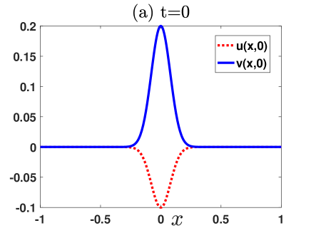
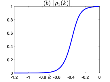
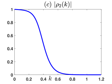
Figure 2. (a) The images of initial condition $u(x,0)$ and $v(x,0)$ in (1.13). (b) The absolute value of reflection coefficient $\rho_{1}(k)$ for $k<0$. (c) The absolute value of reflection coefficient $\rho_{2}(k)$ for $k>0$.

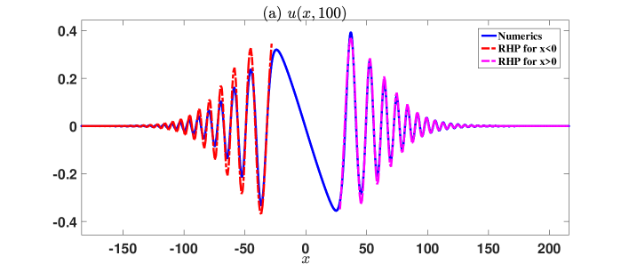
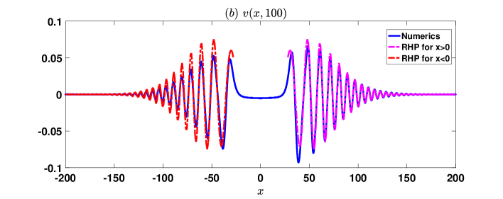
Figure 3. The comparisons of asymptotic expressions given in Theorem 1.1 and full numerical simulations of the Hirota-Satsuma equation (1.2) with initial condition (1.13) at time $t=100$.

Theorem 1.1.

Let $\{u(x,t),v(x,t)\}$ be Schwartz class solution of the Hirota-Satsuma equation (1.2) with initial value $u_{0}=u(x,0),v_{0}=v(x,0)\in\mathcal{S}(\mathbb{R})$ and assume the elements $s_{11}(k)\neq 0$ and $s^{A}_{11}(k)\neq 0$ for $k\in\bar{D}_{4}\setminus\{0\}$ and $k\in\bar{D}_{1}\setminus\{0\}$, respectively, and

$$\lim\limits_{k\to 0}ks_{11}(k)\neq 0,\quad\lim\limits_{k\to 0}ks_{11}^{A}(k)\neq 0,$$

such that the functions $\rho_{1}(k)$ and $\rho_{2}(k)$ in (2.43) satisfy $\rho_{1}(0)=\rho_{2}(0)=\omega$, $|\rho_{1}(k)|<1$ for $k<0$ and $|\rho_{2}(k)|<1$ for $k>0$, then the large-time solution of the Hirota-Satsuma equation (1.2) holds

1. For $\eta=x/t>0$, as $t\to\infty$, the asymptotic behaviors of $u(x,t)$ and $v(x,t)$ are

   $$u(x,t) =-\frac{3^{5/4}\sqrt{2\mu}}{\sqrt{t}}\cos\big{(}\mu\ln(6\sqrt{3}tk_{0}^{2})+\frac{1}{\pi}\int^{-\infty}_{k_{0}}\ln{\frac{|s-k_{0}|}{|s-\omega k_{0}|}}d\ln(1-|\rho_{1}|^{2})$$ (1.10)

   $$-\sqrt{3}tk_{0}^{2}+\frac{3\pi}{4}-\arg{p}-\arg{\Gamma(i\mu)}\big{)}+O(\ln{(t)}/t),$$

   $$v(x,t) =\frac{3^{5/4}\times\sqrt{2\mu}k_{0}}{\sqrt{t}}\sin\big{(}\mu\ln(6\sqrt{3}tk_{0}^{2})+\frac{1}{\pi}\int^{-\infty}_{k_{0}}\ln{\frac{|s-k_{0}|}{|s-\omega k_{0}|}}d\ln(1-|\rho_{1}|^{2})$$

   $$-\sqrt{3}tk_{0}^{2}+\frac{19\pi}{12}-\arg{p}-\arg{\Gamma(i\mu)}\big{)}+O(\ln{(t)}/t),$$

   where $\mu=-\frac{1}{2\pi}\ln(1-|\rho_{1}(k_{0})|^{2})$ and $p=\rho_{1}(k_{0})$ with $k_{0}=-x/(2t).$

1. For $\eta=x/t<0$, as $t\to\infty$, the asymptotic behaviors of $u(x,t)$ and $v(x,t)$ are

   $$u(x,t) =\frac{3^{5/4}\sqrt{2\tilde{\mu}}}{\sqrt{t}}\cos\big{(}\tilde{\mu}\ln(6\sqrt{3}tk_{0}^{2})+\frac{1}{\pi}\int^{\infty}_{k_{0}}\ln{\frac{|s-k_{0}|}{|s-\omega k_{0}|}}d\ln(1-|\rho_{2}|^{2})$$ (1.11)

   $$-\sqrt{3}tk_{0}^{2}+\frac{3\pi}{4}-\arg{\tilde{p}}-\arg{\Gamma(i\tilde{\mu})}\big{)}+O(\ln{(t)}/t),$$

   $$v(x,t) =\frac{3^{5/4}\times\sqrt{2\tilde{\mu}}k_{0}}{\sqrt{t}}\sin\big{(}\tilde{\mu}\ln(6\sqrt{3}tk_{0}^{2})+\frac{1}{\pi}\int^{\infty}_{k_{0}}\ln{\frac{|s-k_{0}|}{|s-\omega k_{0}|}}d\ln(1-|\rho_{2}|^{2})$$

   $$-\sqrt{3}tk_{0}^{2}+\frac{19\pi}{12}-\arg{\tilde{p}}-\arg{\Gamma(i\tilde{\mu})}\big{)}+O(\ln{(t)}/t).$$

   where $\tilde{\mu}=-\frac{1}{2\pi}\ln(1-|\rho_{2}(k_{0})|^{2})$ and $\tilde{p}=\rho_{1}(-k_{0})$.

Proof.

See Section 4.

∎

The large-time asymptotic behavior of the equation (1.4) with Schwartz class initial value has been studied in Charlier, Lenells and Wang [9]. However, thanks to the Miura transformation (3.10) below, a similar asymptotic result can be given in the theorem as follows.

Theorem 1.2.

Let $w(x,t)$ be a solution in the Schwartz class of the good Boussinesq equation (1.4) with initial value $w_{0}=w(x,0)\in\mathcal{S}(\mathbb{R})$. Assume the conditions stated in Theorem 1.1 are satisfied. Then the Miura transformation $w=-\frac{1}{6}u^{2}-\frac{1}{2}v$ and Theorem 1.1 yield the large-time solution of the good Boussinesq equation (1.4) for $\eta=x/t>0$ as follows

$$w(x,t) =-\frac{3^{5/4}\times\sqrt{\mu}k_{0}}{\sqrt{2t}}\sin\big{(}\mu\ln(6\sqrt{3}tk_{0}^{2})+\frac{1}{\pi}\int^{-\infty}_{k_{0}}\ln{\frac{|s-k_{0}|}{|s-\omega k_{0}|}}d\ln(1-|\rho_{1}|^{2})$$ (1.12)

$$-\sqrt{3}tk_{0}^{2}+\frac{19\pi}{12}-\arg{p}-\arg{\Gamma(i\mu)}\big{)}+O(\ln{(t)}/t),\quad t\to\infty,$$

where $\mu(\eta)=-\frac{1}{2\pi}\ln(1-|\rho_{1}(k_{0})|^{2})$ and $p=\rho_{1}(k_{0})$ with $k_{0}=-x/(2t).$

In order to check the validity of the long-time asymptotics of the Hirota-Satsuma equation (1.2) in Theorem 1.1, take the initial value of the form

$$u(x,0)=-0.1e^{-x^{2}/20},\quad v(x,0)=0.2e^{-x^{2}/20},$$ (1.13)

which are Gaussian wave packets shown in Figure 2(a). Under this initial condition, Figure 2(b)-(c) demonstrate the modulus of the functions $\rho_{1}(k)$ and $\rho_{2}(k)$, which are reflection coefficients. It is seen that $|\rho_{1}(0)|=1,\lim\limits_{k\to-\infty}\rho_{1}(k)=0,|\rho_{1}(k)|<1$ for $k<0$ and $|\rho_{2}(0)|=1,\lim\limits_{k\to+\infty}\rho_{2}(k)=0,|\rho_{2}(k)|<1$ for $k>0$. Figure 3 shows the comparison of asymptotic expressions given in Theorem 1.1 with numerical simulations with initial condition (1.13) at $t=100$, in which the dashed pink and red lines correspond to the asymptotic expressions in (1.10) and (1.11) while the blue solid lines represent the numerical results. Expectedly, the large-time asymptotic solutions can approximate the numerical solutions within certain error range.

2. Direct and inverse spectral problem

This section mainly builds the direct and inverse spectral theory of Lax pair (1.3) and proposes the Riemann-Hilbert problem associated with the solution $u$ and $v$ of the Hirota-Satsuma equation (1.2).

2.1. The modified Lax pair

For $k\in\mathbb{C}\setminus\{0\}$, define $\psi=P\phi$, where

$$P(k)=\begin{pmatrix}\omega k&\omega^{2}k&k\\ \omega^{2}k^{2}&\omega k^{2}&k^{2}\\ 1&1&1\end{pmatrix},\quad\omega=e^{\frac{2i\pi}{3}},$$ (2.1)

with $\det(P(k))=3(\omega^{2}-\omega)k^{3}$, then the Lax pair (1.3) is converted into

$$\begin{cases}\phi_{x}=L\phi,\\ \phi_{t}=Z\phi,\end{cases}$$ (2.2)

with

$$L=P^{-1}\tilde{L}P,\quad Z=P^{-1}\tilde{Z}P.$$

Rewrite $L$ and $Z$ as

$$L=\mathcal{L}+U,\quad Z=\mathcal{Z}+V,$$ (2.3)

with $\mathcal{L}=-kJ$ and $\mathcal{Z}=k^{2}J^{2}$, where $J$ is a diagonal matrix defined by

$$J=\begin{pmatrix}\omega&0&0\\ 0&\omega^{2}&0\\ 0&0&1\end{pmatrix},$$ (2.4)

and $U,V$ take the forms

$$U(x,t,k)=U^{(0)}(x,t)+\frac{1}{k}U^{(-1)}(x,t),$$ (2.5a)

$$V(x,t,k)=kV^{(1)}(x,t)+V^{(0)}(x,t)+\frac{1}{k}V^{(-1)}(x,t),$$ (2.5b)

where

$$U^{(0)} =\frac{u}{3}\begin{pmatrix}0&\omega^{2}&\omega\\ \omega&0&\omega^{2}\\ \omega^{2}&\omega&0\end{pmatrix},\quad U^{(-1)}=-\frac{v}{3}\begin{pmatrix}\omega^{2}&1&\omega\\ 1&\omega&\omega^{2}\\ \omega&\omega^{2}&1\end{pmatrix},$$

$$V^{(1)} =\frac{u}{3}\begin{pmatrix}0&\omega^{2}&1\\ \omega&0&1\\ \omega&\omega^{2}&0\end{pmatrix},\quad V^{(-1)}=\frac{2u_{xx}-uv-3v_{x}}{9}\begin{pmatrix}\omega^{2}&1&\omega\\ 1&\omega&\omega^{2}\\ \omega&\omega^{2}&1\end{pmatrix},$$

$$V^{(0)} =\frac{1}{9}\begin{pmatrix}0&\omega^{2}u^{2}+(1-\omega)u_{x}-3v&\omega u^{2}+(\omega+2)u_{x}-3v\\ \omega u^{2}-3v+(\omega+2)u_{x}&0&\omega^{2}u^{2}+(1-\omega)u_{x}-3v\\ \omega^{2}u^{2}-3v+(1-\omega)u_{x}&\omega u^{2}-3v+(\omega+2)u_{x}&0\end{pmatrix}.$$

Direct calculations show that $L$ and $Z$ satisfy the $\mathbb{Z}_{2}$ and $\mathbb{Z}_{3}$ symmetries below, respectively

$$L(k)=\mathcal{B}\overline{L(\bar{k})}\mathcal{B},\quad{\rm and}\quad Z(k)=\mathcal{B}\overline{Z(\bar{k})}\mathcal{B},\quad\mathcal{B}=\begin{pmatrix}0&1&0\\ 1&0&0\\ 0&0&1\end{pmatrix},$$ (2.6)

$$L(k)=\mathcal{A}L(\omega k)\mathcal{A}^{-1},\quad{\rm and}\quad Z(k)=\mathcal{A}Z(\omega k)\mathcal{A}^{-1},\quad\mathcal{A}=\begin{pmatrix}0&0&1\\ 1&0&0\\ 0&1&0\end{pmatrix}.$$ (2.7)

The decomposition (2.5) and the transformation $\phi=Ye^{\mathcal{L}x+\mathcal{Z}t}$ turn the Lax pair (2.2) into the modified Lax pair

$$\begin{cases}Y_{x}-[\mathcal{L},Y]=UY,\\ Y_{t}-[\mathcal{Z},Y]=VY.\end{cases}$$ (2.8)

2.2. The eigenfunctions $Y_{1}$ and $Y_{2}$

Fixing time $t$, we are particularly interested in the $x$-part of the modified Lax pair (2.8), i.e.,

$$Y_{x}-[\mathcal{L},Y]=UY.$$ (2.9)

For convenience, rewrite $\mathcal{L}=\text{diag\,}\{l_{1},l_{2},l_{3}\}$ with $l_{j}=-k\omega^{j}$ $(j=1,2,3)$ and $\mathcal{Z}=\text{diag\,}\{z_{1},z_{2},z_{3}\}$ with $z_{j}=k^{2}\omega^{2j}$ $(j=1,2,3)$. Then the complex $k$-plane is decomposed into six open sets $\{\Omega_{n}\}_{1}^{6}$ in Fig. 4, where we have set $S=\{k\in\mathbb{C}|\arg{k}\in(-\frac{\pi}{3},\frac{\pi}{3})\}$, which denotes the interior of $\bar{\Omega}_{6}\cup\bar{\Omega}_{1}$.

Figure 4. The jump contour $\Gamma=\cup_{i=1}^{6}\Gamma_{i}$ and six open sets $\Omega_{j},j=1,\dots,6$.

Define two three-order matrix-valued eigenfunctions $Y_{1}$ and $Y_{2}$ as the solutions to the Volterra integral equations

$$Y_{1}(x,k)=I-\int_{x}^{\infty}e^{\left(x-s\right)\widehat{\mathcal{L}(k)}}(U(s,k)Y_{1}\left(s,k\right))ds,$$ (2.10a)

$$Y_{2}(x,k)=I+\int_{-\infty}^{x}e^{\left(x-s\right)\widehat{\mathcal{L}(k)}}(U(s,k)Y_{2}\left(s,k\right))ds,$$ (2.10b)

where $e^{\left(x-s\right)\widehat{\mathcal{L}(k)}}(UY)=e^{\left(x-s\right)\mathcal{L}(k)}UYe^{-\left(x-s\right)\mathcal{L}(k)}$. Letting $\mathcal{S}\left(\mathbb{R}\right)$ be the Schwartz space, the properties of the eigenfunctions $Y_{1}$ and $Y_{2}$ are given in the next proposition.

Proposition 2.1.

Denote $\Xi=(\omega^{2}\bar{S},\omega\bar{S},\bar{S})$ and $\hat{\Xi}=(-\omega^{2}\bar{S},-\omega\bar{S},-\bar{S})$. If $u_{0},v_{0}\in\mathcal{S}\left(\mathbb{R}\right)$, the matrix-valued solutions $Y_{1}(x,k)$ and $Y_{2}(x,k)$ of (2.9) exhibit the following characteristics:

1. The function $Y_{1}(x,k)$ is well-defined for $x\in\mathbb{R}$ and for $k$ belonging to the region $\Xi$ excluding zero. Additionally, $Y_{1}(\cdot,k)$ is smooth for any $k$ within this region excluding zero.

1. The function $Y_{2}(x,k)$ is well-defined for $x\in\mathbb{R}$ and for $k$ belonging to the region $\hat{\Xi}$ excluding zero. Additionally, $Y_{2}(\cdot,k)$ is smooth for any $k$ within this region excluding zero.

1. For given $x\in\mathbb{R}$, $Y_{1}(x,\cdot)$ is analytic for any $k\in\Xi\setminus\{0\}$.

1. For given $x\in\mathbb{R}$, $Y_{2}(x,\cdot)$ is analytic for any $k\in\hat{\Xi}\setminus\{0\}$.

1. The partial derivative $\frac{\partial^{i}Y_{1}}{\partial k^{i}}(x,\cdot)$ can extend continuously to $k\in\Xi\setminus\{0\}$ for any $x\in\mathbb{R}$ and each integer $i\geq 1$.

1. The partial derivative $\frac{\partial^{i}Y_{2}}{\partial k^{i}}(x,\cdot)$ can extend continuously to $k\in\hat{\Xi}\setminus\{0\}$ for any $x\in\mathbb{R}$ and each integer $i\geq 1$.

1. For any integer $n\geq 1$, there exist two bounded, smooth, positive functions $g_{1}(x)$ and $g_{2}(x)$ defined on $x\in\mathbb{R}$, which decay rapidly as $x$ approaches $\infty$ and $-\infty$, respectively, such that

   $$\left|\frac{\partial^{i}}{\partial k^{i}}(Y_{1}(x,k)-I)\right|\leq g_{1}(x),\quad k\in\Xi\setminus\{0\},\quad i=0,1,2\cdots,n,$$ (2.11a)

   $$\left|\frac{\partial^{i}}{\partial k^{i}}(Y_{2}(x,k)-I)\right|\leq g_{2}(x),\quad k\in\hat{\Xi}\setminus\{0\},\quad i=0,1,2\cdots,n.$$ (2.11b)

1. For any $x\in\mathbb{R}$, the eigenfunctions $Y_{1}$ and $Y_{2}$ also satisfy the $\mathbb{Z}_{2}$ and $\mathbb{Z}_{3}$ symmetries

   $$Y_{1}(x,k)=\mathcal{A}Y_{1}(x,\omega k)\mathcal{A}^{-1}=\mathcal{B}\overline{Y_{1}(x,\bar{k})}\mathcal{B},\quad k\in\Xi\setminus\{0\},$$ (2.12a)

   $$Y_{2}(x,k)=\mathcal{A}Y_{2}(x,\omega k)\mathcal{A}^{-1}=\mathcal{B}\overline{Y_{2}(x,\bar{k})}\mathcal{B},\quad k\in\hat{\Xi}\setminus\{0\}.$$ (2.12b)

1. Suppose $u_{0},v_{0}$ are supported compactly. For every $x\in\mathbb{R}$ and $k\in\mathbb{C}\setminus\{0\}$, both $Y_{1}(x,k)$ and $Y_{2}(x,k)$ are analytic, and their determinants are equal to $1$: $\det{Y_{1}(x,k)}=\det{Y_{2}(x,k)}=1$.

2.3. Asymptotics of the eigenfunctions $Y_{1}$ and $Y_{2}$ as $k\to\infty$

The differential equation (2.9) allows the formal solutions

$$Y_{1}^{formal}(x,k)=I+\frac{Y_{1}^{(1)}(x)}{k}+\frac{Y_{1}^{(2)}(x)}{k^{2}}+\dots,$$

$$Y_{2}^{formal}(x,k)=I+\frac{Y_{2}^{(1)}(x)}{k}+\frac{Y_{2}^{(2)}(x)}{k^{2}}+\dots,$$

in which the coefficients satisfy

$$\lim_{x\to+\infty}Y_{1}^{(j)}(x)=\lim_{x\to-\infty}Y_{2}^{(j)}(x)=0,\quad j\geq 1.$$

For convenience, rewrite the matrix $U(x,k)$ as

$$U(x,k)=U_{0}(x)+\frac{U_{1}(x)}{k},$$

with

$$U_{0}(x)=U^{(0)}(x,0),\qquad U_{1}(x)=U^{(-1)}(x,0).$$

Inserting

$$Y_{1}=I+\frac{Y_{1}^{(1)}(x)}{k}+\frac{Y_{1}^{(2)}(x)}{k^{2}}+\cdots$$

into the equation (2.9) yields

$$\begin{cases}[J,Y_{1}^{(j+1)}]=-\partial_{x}(Y_{1}^{(j)})^{(o)}+(U_{0}Y_{1}^{(j)}+U_{1}Y_{1}^{(j-1)})^{(o)},\\ \partial_{x}(Y_{1}^{(j+1)})^{(d)}=(U_{0}Y_{1}^{(j+1)}+U_{1}Y_{1}^{(j)})^{(d)},\end{cases}$$

in which $Y^{(d)}$ denotes the diagonal parts of the matrix $Y$ and $Y^{(o)}$ denotes the off-diagonal parts. Some calculations give the first coefficient of $Y_{1}$ of the form

$$Y_{1}^{(1)}(x)=-\int_{\infty}^{x}\frac{u^{2}_{0}(x^{\prime})+3v_{0}(x^{\prime})}{9}\begin{pmatrix}\omega^{2}&0&0\\ 0&\omega&0\\ 0&0&1\end{pmatrix}dx^{\prime}-\frac{u_{0}}{9}\begin{pmatrix}0&-\omega(\omega+2)&\omega(\omega+2)\\ \omega+2&0&-(\omega+2)\\ -\omega^{2}(\omega+2)&\omega^{2}(\omega+2)&0\end{pmatrix}.$$

Proposition 2.2.

Let $u_{0},v_{0}\in\mathcal{S}(\mathbb{R})$, then when $k\to{\infty}$, $Y_{1}$ and $Y_{2}$ approximate to $Y_{1}^{formal}$ and $Y_{2}^{formal}$, respectively. Furthermore, assuming $p\geq 0$ is an integer, define two functions

$$Y_{1,p}(x,k): =I+\frac{Y_{1}^{(1)}(x)}{k}+\cdots+\frac{Y_{1}^{(p)}(x)}{k^{p}},$$ (2.13a)

$$Y_{2,p}(x,k): =I+\frac{Y_{2}^{(1)}(x)}{k}+\cdots+\frac{Y_{2}^{(p)}(x)}{k^{p}}.$$ (2.13b)

Then there exist two bounded, smooth, positive functions $g_{1}(x)$ and $g_{2}(x)$ defined for $x\in\mathbb{R}$, which decay rapidly as $x$ approaches $\infty$ and $-\infty$, respectively, such that

$$\left|\frac{\partial^{i}}{\partial k^{i}}\left(Y_{1}-Y_{1,p}\right)\right|\leq\frac{g_{1}(x)}{|k|^{p+1}},\quad k\in\Xi,\quad|k|\geq 2,$$ (2.14a)

$$\left|\frac{\partial^{i}}{\partial k^{i}}\left(Y_{2}-Y_{2,p}\right)\right|\leq\frac{g_{2}(x)}{|k|^{p+1}},\quad k\in\hat{\Xi},\quad|k|\geq 2,$$ (2.14b)

for any $x\in\mathbb{R}$ and $i=0,1,2,\cdots.$

2.4. Asymptotics of the eigenfunctions $Y_{1}$ and $Y_{2}$ as $k\to 0$

The eigenfunctions $Y_{1}$ and $Y_{2}$ have a first-order pole at $k=0$ because the function $U(x,t,k)$ in (2.5a) has a first-order pole, which is caused by the gauge transformation (2.1). In such case, the following proposition holds near the origin $k=0$.

Proposition 2.3.

Let $u_{0},v_{0}\in\mathcal{S}(\mathbb{R})$ and integer $p\geq 0$. There are third-order matrix-valued functions $C_{i}^{(l)}(x)$ for $i=1,2;l=-1,0,\dots,p$, which satisfy

1. For each $x\in\mathbb{R}$, there exist two smooth functions $g_{1}(x)>0$ and $g_{2}(x)>0$ which decay rapidly as $x\to{\infty}$ and $x\to{-\infty}$ respectively, such that

   $$\left|\frac{\partial^{j}}{\partial k^{j}}(Y_{1}-I-\sum_{l=-1}^{p}C_{1}^{(l)}(x)k^{l})\right|\leq g_{1}(x)|k|^{p+1-j},\quad k\in\Xi,\quad|k|\leq\frac{1}{2},$$ (2.15a)

   $$\left|\frac{\partial^{j}}{\partial k^{j}}(Y_{2}-I-\sum_{l=-1}^{p}C_{2}^{(l)}(x)k^{l})\right|\leq g_{2}(x)|k|^{p+1-j},\quad k\in\hat{\Xi},\quad|k|\leq\frac{1}{2},$$ (2.15b)

   where $j\geq 0$ is an integer.

1. The functions $C_{1}^{(l)}$ and $C_{2}^{(l)}$ are smooth and decay rapidly as $x\to{\infty}$ and $x\to{-\infty}$ respectively for $l=-1,0,1,2,\cdots$.

1. The leading coefficients are given by

   $$C_{i}^{(-1)}(x)= \alpha_{i}(x)\begin{pmatrix}\omega^{2}&1&\omega\\ 1&\omega&\omega^{2}\\ \omega&\omega^{2}&1\end{pmatrix},$$ (2.16)

   $$C_{i}^{(0)}(x)= \beta_{i}(x)\begin{pmatrix}1&\omega^{2}&\omega\\ \omega&1&\omega^{2}\\ \omega^{2}&\omega&1\end{pmatrix}+\gamma_{i}(x)\begin{pmatrix}1&\omega&\omega^{2}\\ \omega^{2}&1&\omega\\ \omega&\omega^{2}&1\end{pmatrix}+\delta_{i}(x)\begin{pmatrix}1&1&1\\ 1&1&1\\ 1&1&1\end{pmatrix}-I,$$ (2.17)

   where functions $\alpha_{i}(x),\beta_{i}(x),\gamma_{i}(x),\delta_{i}(x),i=1,2$ are real-valued. Moreover, they satisfy

   $$|\alpha_{i}(x)|\leq(1+|x|)g_{i}(x),$$

   $$|\beta_{i}(x)|+|\gamma_{i}(x)|\leq(1+|x|)^{2}g_{i}(x),$$

   $$|\delta_{i}(x)-\frac{1}{3}|\leq(1+|x|)^{2}g_{i}(x),$$

   for $x\in\mathbb{R}$ and $i=1,2$.

Proof.

Let us define $\tilde{Y}(x,k)=P(k)Y_{1}(x,k)$ that satisfies

$$\tilde{Y}(x,k)=P(k)-\int_{x}^{\infty}P(k)e^{\left(x-s\right)\widehat{\mathcal{L}}}\left(P(k)^{-1}\tilde{\mathrm{U}}\left(s\right)\tilde{Y}\left(s,k\right)\right)ds,$$ (2.18)

for $x\in\mathbb{R}$ and $k\in\Xi\backslash\{0\}$, where the matrix $\tilde{U}$ is of the form

$$\tilde{U}:=PUP^{-1}=\begin{pmatrix}-\frac{1}{3}u_{0}&0&0\\ -v_{0}&\frac{2}{3}u_{0}&0\\ 0&0&-\frac{1}{3}u_{0}\end{pmatrix}.$$ (2.19)

Firstly, we prove that the first two lines in $\tilde{Y}(x,0)$ are zero. Assume that $\mathcal{P}\left(x,s,k\right):=P(k)e^{\left(x-s\right)\mathcal{L}(k)}P(k)^{-1}$. By computing the behavior at the zero, we can get $k=0$ is a removable singularity of $\mathcal{P}$. In other word, $\mathcal{P}$ is analytic at $k=0$. Now the kernel of Volterra integral function $\tilde{Y}(x,k)$ loses the singularity at $k=0$. Thus following the same procedure in the Proposition 2.1, $\tilde{Y}(x,k)$ is analytic at $k=0$. Rewrite the Taylor expansion of $\tilde{Y}(x,k)$ at $k=0$ as

$$\tilde{Y}(x,k)=\tilde{Y}(x,0)+\partial_{k}\tilde{Y}(x,0)k+\frac{1}{2}\partial_{k}^{2}\tilde{Y}(x,0)k^{2}+\cdots,\quad k\to 0,\quad k\in\Xi,$$

in which the coefficients are smooth of $x$ in the real domain. As $x$ approaches $+\infty$, the derivatives $\partial_{k}^{j}\tilde{Y}(x,k)$ converge rapidly to $\partial_{k}^{j}P(k)$ for each $j\geq 0$ and $k\in\Xi$. Let us analyze the behavior of $\partial_{k}^{j}\tilde{Y}(x,0)~{}(j=0,1,2)$, as $x\rightarrow-\infty$. It can be calculated that

$$\mathcal{P}\left(x,s,0\right)=\begin{pmatrix}1&s-x&0\\ 0&1&0\\ s-x&\frac{(s-x)^{2}}{2}&1\end{pmatrix}.$$

By means of the equation (2.19), it follows

$$\mathcal{P}\left(x,s,0\right)\tilde{U}\left(s\right)=\begin{pmatrix}-\frac{u_{0}(s)}{3}-v_{0}(s)(s-x)&\frac{2u_{0}(s)}{3}(s-x)&0\\ -v_{0}(s)&\frac{2}{3}u_{0}(s)&0\\ -\frac{u_{0}(s)}{3}(s-x)-\frac{v_{0}(s)}{2}(s-x)^{2}&\frac{u_{0}(s)}{3}(x-s)^{2}&-\frac{u_{0}(s)}{3}\end{pmatrix},$$

and further

$$\mathcal{P}\left(x,s,0\right)\tilde{U}\left(s\right)P(0)=\begin{pmatrix}0&0&0\\ 0&0&0\\ -\frac{u_{0}(s)}{3}&-\frac{u_{0}(s)}{3}&-\frac{u_{0}(s)}{3}\end{pmatrix}.$$

Therefore, we have proved that the first two lines in $\tilde{Y}(x,0)$ are zero by analyzing the volterra equation (2.18) and found the behavior of $\tilde{Y}(x,0)$ as $x\to-\infty$, i.e.,

$$\tilde{Y}(x,0)=\begin{pmatrix}O(x)&O(x)&O(x)\\ O(1)&O(1)&O(1)\\ O(x^{2})&O(x^{2})&O(x^{2})\end{pmatrix},\qquad\text{as}\quad x\to-\infty.$$

Similarly, it is estimated that as $x\to-\infty$

$$\partial_{k}\tilde{Y}(x,0)=\begin{pmatrix}O(x^{2})&O(x^{2})&O(x^{2})\\ O(x)&O(x)&O(x)\\ O(x^{3})&O(x^{3})&O(x^{3})\end{pmatrix},\quad\partial^{2}_{k}\tilde{Y}(x,0)=\begin{pmatrix}O(x^{3})&O(x^{3})&O(x^{3})\\ O(x^{2})&O(x^{2})&O(x^{2})\\ O(x^{4})&O(x^{4})&O(x^{4})\end{pmatrix}.$$

Next, we prove that $Y_{1}(x,k)$ has only first-order pole at $k=0$. To do so, it is obvious that $P(k)^{-1}$ has the form

$$P(k)^{-1}=\frac{P^{(-2)}}{k^{2}}+\frac{P^{(-1)}}{k}+P^{(0)},$$

where

$$P^{(-2)}=\frac{1}{3}\begin{pmatrix}0&\omega&0\\ 0&\omega^{2}&0\\ 0&1&0\end{pmatrix},\quad P^{(-1)}=\frac{1}{3}\begin{pmatrix}\omega^{2}&0&0\\ \omega&0&0\\ 1&0&0\end{pmatrix},\quad P^{(0)}=\frac{1}{3}\begin{pmatrix}0&0&1\\ 0&0&1\\ 0&0&1\\ \end{pmatrix},$$

which indicates that $Y_{1}(x,k)=P^{-1}(k)\tilde{Y}(x,k)$ possesses at most one double pole located at $k=0$. So set

$$Y_{1}(x,k)=\frac{C_{1}^{(-2)}(x)}{k^{2}}+\frac{C_{1}^{(-1)}(x)}{k}+I+C_{1}^{(0)}(x)+C_{1}^{(1)}(x)k+\cdots,\quad k\in\Xi,$$

as $k\to 0$. Direct calculations show that

$$C_{1}^{(-2)}(x) =P^{(-2)}\tilde{Y}(x,0)=0,$$

$$C_{1}^{(-1)}(x) =P^{(-2)}\partial_{k}\tilde{Y}(x,0)+P^{(-1)}\tilde{Y}(x,0)=P^{(-2)}\partial_{k}\tilde{Y}(x,0),$$

$$C_{1}^{(0)}(x) =\frac{1}{2}P^{(-2)}\partial_{k}^{2}\tilde{Y}(x,0)+P^{(-1)}\partial_{k}\tilde{Y}(x,0)+P^{(0)}\tilde{Y}(x,0)-I.$$

Assume that

$$\partial_{k}\tilde{Y}(x,0)=\begin{pmatrix}a_{11}(x)&a_{12}(x)&a_{13}(x)\\ a_{21}(x)&a_{22}(x)&a_{23}(x)\\ a_{31}(x)&a_{32}(x)&a_{33}(x)\end{pmatrix},$$

where the functions $a_{ij}(x)~{}(i,j=1,2,3)$ are complex. Due to the special form of matrix $P^{(-2)}$, it follows

$$C_{1}^{(-1)}(x)=\frac{1}{3}\begin{pmatrix}\omega a_{21}&\omega a_{22}&\omega a_{23}\\ \omega^{2}a_{21}&\omega^{2}a_{22}&\omega^{2}a_{23}\\ a_{21}&a_{22}&a_{23}\end{pmatrix}.$$

The symmetries in (2.12) indicate that $a_{21}=\omega^{2}a_{22}=\omega a_{23}$ and $a_{23}=\bar{a}_{23}$. Thus we have completed the proof of (2.16) with $\alpha_{1}(x)=\frac{1}{3}a_{23}$. The proof of $C_{1}^{(0)}$ in (2.36) and the asymptotics for $Y_{2}$ can also be given similarly.

∎

2.5. The scaterring data $s(k)$

The functions $Y_{1}$ and $Y_{2}$ are linearly dependent as both of them are the solutions of the equation (2.9). Therefore, for $u_{0},v_{0}\in\mathcal{S}(\mathbb{R})$, one can set

$$Y_{1}(x,k)=Y_{2}(x,k)e^{x\widehat{\mathcal{L}(k)}}s(k),$$ (2.20)

for $x\in\mathbb{R}$ and $k\in\mathbb{C}\setminus\{0\}$. From the properties of the Volterra integral equations (2.10) at $x=-\infty$, it follows

$$s(k)=I-\int_{-\infty}^{\infty}e^{-x\widehat{\mathcal{L}(x)}}\left(UY_{1}\right)\left(x,k\right)dx.$$ (2.21)

Recalling the Proposition 2.1, the following proposition can be given at once.

Proposition 2.4.

Amussing $u_{0},v_{0}\in\mathcal{S}(\mathbb{R})$, the scaterring matrix $s(k)$ satisfies

1. The matrix $s(k)$ is well-defined and continuous on

   $$k\in\begin{pmatrix}\omega^{2}\bar{S}&\mathbb{R}^{-}&\omega\mathbb{R}^{-}\\ \mathbb{R}^{-}&\omega\bar{S}&\omega^{2}\mathbb{R}^{-}\\ \omega\mathbb{R}^{-}&\omega^{2}\mathbb{R}^{-}&\bar{S}\end{pmatrix}\backslash\{0\}.$$ (2.22)

   For example, the entry $s_{11}$ is well-defined and continuous for $k\in\omega^{2}\bar{S}\backslash\{0\}$.

1. The spectral function $s(k)$ admits the symmetries

   $$s(k)=\mathcal{A}s(\omega k)\mathcal{A}^{-1}=\mathcal{B}\overline{s(\bar{k})}\mathcal{B}.$$ (2.23)

1. The arbitrary-order derivative $\partial_{k}^{j}s(k)~{}(j>0)$ is continuous for $k$ in (2.22).

1. For $k$ in (2.22) and $k$ tends to infinity, $s(k)$ converges to the identity matrix. Moreover, for any integer $N\geq 1$ and $k$ in (2.22), we have

   $$\left|\partial_{k}^{j}\left(s(k)-I-\sum_{j=1}^{N}\frac{s_{j}}{k^{j}}\right)\right|=O\left(k^{-N-1}\right),\quad k\to\infty,\quad j=0,1,2,\cdots,N,$$ (2.24)

   where $\{s_{j}\}_{1}^{\infty}$ are diagonal matrices.

1. For $k$ in (2.22) and $k\to 0$, it is seen that

   $$s(k)=\frac{s^{(-1)}}{k}+s^{(0)}+s^{(1)}k+\ldots,$$ (2.25)

   where

   $$s^{(-1)}=\mathrm{s}^{(-1)}\left(\begin{array}[]{ccc}\omega^{2}&1&\omega\\ 1&\omega&\omega^{2}\\ \omega&\omega^{2}&1\end{array}\right),\quad\mathrm{s}^{(-1)}:=-\int_{\mathbb{R}}(\frac{2}{3}\alpha_{1}(x)u_{0}-v_{0}\gamma_{1}(x))dx.$$ (2.26)

1. If $u_{0}(x),v_{0}(x)$ are compactly supported, the function $s(k)$ is analytic for $k\in\mathbb{C}\backslash\{0\}$ and $\det{s}=1$.

Proof.

Property (1) can be obtained by direct calculation where it is ensured that the exponential factors are bounded. The properties (2) and (3) are obvious from the properties of $Y_{1}$ in Proposition 2.1. Recalling that $Y_{1}$ has good properties in Proposition 2.2, for $k$ in (2.22), we have

$$s(k)=I-\sum_{j=0}^{p}\frac{1}{k^{j}}\int_{\mathbb{R}}e^{-x\widehat{\mathcal{L}(k)}}\big{(}U(x,k)Y_{1}^{(p)}(x)\big{)}dx+O(k^{-p-1}),$$

as $k\to\infty$. Note that $U(\cdot,k)\in\mathcal{S}(\mathbb{R})$ and $Y_{1}^{(p)}(x)$ and their derivatives are bounded. Then the integration by parts applied to the off-diagonal elements of $s(k)$ shows that $\{s_{j}\}_{1}^{\infty}$ are diagonal matrices as $k\to\infty$. With $\tilde{U}$ and $\tilde{Y}$ defined in the proof of Proposition 2.3, rewrite $s(k)$ as

$$s(k) =I-\int_{-\infty}^{\infty}e^{-x\widehat{\mathcal{L}(k)}}\big{(}P(k)^{-1}\tilde{U}(x)\tilde{Y}(x,k)\big{)}dx$$

$$=I-\int_{-\infty}^{\infty}e^{-x\widehat{\mathcal{L}(k)}}\big{[}(\frac{P^{(-2)}}{k^{2}}+\frac{P^{(-1)}}{k}+P^{(0)})\tilde{U}\left(\tilde{Y}(x,0)+\partial_{k}\tilde{Y}(x,0)k+\cdots\right)\big{]}dx$$

$$=I-\frac{1}{k^{2}}\int_{-\infty}^{\infty}e^{-x\widehat{\mathcal{L}(k)}}P^{(-2)}\tilde{U}\tilde{Y}(x,0)dx$$

$$-\frac{1}{k}\int_{-\infty}^{\infty}e^{-x\widehat{\mathcal{L}(k)}}[P^{(-2)}\tilde{U}\partial_{k}\tilde{Y}(x,0)+P^{(-1)}\tilde{U}\tilde{Y}(x,0)]dx+\cdots$$

$$=I-\frac{1}{k}\int_{-\infty}^{\infty}e^{-x\widehat{\mathcal{L}(k)}}[P^{(-2)}\tilde{U}\partial_{k}\tilde{Y}(x,0)]dx+\cdots$$

$$=\frac{s^{(-1)}}{k}+s^{(0)}+s^{(1)}k+\cdots,$$

where we have used the fact that only the last line in the matrix $\tilde{Y}(x,0)$ is not zero, and the coefficient $s^{(-1)}$ is

$$s^{(-1)}=-\int_{-\infty}^{\infty}e^{-x\widehat{\mathcal{L}(k)}}[P^{(-2)}\tilde{U}\partial_{k}\tilde{Y}(x,0)]dx.$$ (2.27)

In fact, the coefficient $s^{(-1)}$ takes the following form

$$s^{(-1)}=-\int_{-\infty}^{\infty}P^{(-2)}\tilde{U}\partial_{k}\tilde{Y}(x,0)dx.$$ (2.28)

The diagonal elements in the right-hand side of (2.27) is the same as the right-hand side of (2.28). Next it needs to show that off-diagonal elements in (2.27) and (2.28) are also equal. For simplicity, only the $(12)$ entry of $s^{(-1)}$ in (2.27) and (2.28) is verified to the same (the other off-diagonal elements can be estimated similarly). As $l_{1}(k)-l_{2}(k)=-\sqrt{3}\mathrm{i}k$, it follows

$$\big{|}\int_{\mathbb{R}}(e^{-x(l_{1}-l_{2})}-1)f(x)dx\big{|}\leq\int_{\mathbb{R}}|\sqrt{3}\mathrm{i}kxf(x)|dx=O(k),\qquad k\to 0,$$

for any $f\in\mathcal{S}(\mathbb{R})$. In this sense, one can replace $e^{-x(l_{1}-l_{2})}$ with $1$. Then the calculation of (2.26) is direct.

Providing $u_{0}(x),v_{0}(x)$ are compactly supported, the integral in (2.21) is convergent for $k\in\mathbb{C}\setminus\{0\}$. Therefore, $s(k)$ is well-defined and analytic for $k\in\mathbb{C}\setminus\{0\}$. Furthermore, as $\det{Y_{1}}=\det{Y_{2}}=1$, we have $\det{s}=1$ from (2.20). ∎

2.6. The adjoint eigenfunctions $Y_{1}^{A}(x,k)$ and $Y_{2}^{A}(x,k)$

For a third order matrix $V$ which has a unit determinant, define its cofactor matrix $V^{A}=(V^{-1})^{T}$ in the following form

$$V^{A}=\begin{pmatrix}m_{11}(V)&-m_{12}(V)&m_{13}(V)\\ -m_{12}(V)&m_{22}(V)&-m_{23}(V)\\ m_{31}(V)&m_{32}(V)&m_{33}(V)\end{pmatrix},$$

where $m_{ij}(V)$ represents the $(ij)$th minor of the matrix $V$.

Supposing $u_{0},v_{0}\in\mathcal{S}(\mathbb{R})$ have compact support, the entries of matrices $Y_{1}(x,k),Y_{2}(x,k)$ and $s(k)$ will be defined for $k\in\mathbb{C}\setminus\{0\}$. From the identity $(Y_{1}^{A})_{x}=-Y_{1}^{A}(Y_{1}^{T})_{x}Y_{1}^{A}$ and (2.9), it’s not difficult to find that

$$(Y^{A})_{x}+[\mathcal{L},Y^{A}]=-U^{T}Y^{A}.$$ (2.29)

Since $Y_{1}^{A}\to I$ as $x\to+\infty$ and $Y_{2}^{A}\to I$ as $x\to-\infty$, it is observed that $Y_{1}^{A}$ and $Y_{2}^{A}$ satisfy

$$Y^{A}_{1}(x,k)=I+\int_{x}^{\infty}e^{-(x-s)\widehat{\mathcal{L}(k)}}(U^{T}Y_{1}^{A})(s,k)ds,$$ (2.30a)

$$Y^{A}_{2}(x,k)=I-\int^{x}_{-\infty}e^{-(x-s)\widehat{\mathcal{L}(k)}}(U^{T}Y_{1}^{A})(s,k)ds.$$ (2.30b)

The next proposition on $Y_{1}^{A}(x,k)$ and $Y_{2}^{A}(x,k)$ is similar to Proposition 2.1.

Proposition 2.5.

Assuming $u_{0},v_{0}\in\mathcal{S}\left(\mathbb{R}\right)$, the matrix-valued solutions $Y_{1}^{A}(x,k)$ and $Y_{2}^{A}(x,k)$ of (2.29) satisfy the characteristics as follow:

1. The function $Y_{1}^{A}(x,k)$ is well-defined for $x\in\mathbb{R}$ and for $k$ belonging to the region $\hat{\Xi}$ excluding zero. Additionally, $Y_{1}^{A}(\cdot,k)$ is smooth for any $k$ within this region excluding zero and satisfies (2.29).

1. The function $Y_{2}^{A}(x,k)$ is well-defined for $x\in\mathbb{R}$ and for $k$ belonging to the region $\Xi$ excluding zero. Additionally, $Y_{2}^{A}(\cdot,k)$ is smooth for any $k$ within this region excluding zero and satisfies (2.29).

1. For given $x\in\mathbb{R}$, $Y_{1}^{A}(x,\cdot)$ is continuous and analytic for any $k\in\hat{\Xi}\setminus\{0\}$.

1. For given $x\in\mathbb{R}$, $Y_{2}^{A}(x,\cdot)$ is continuous and analytic for any $k\in\Xi\setminus\{0\}$.

1. The partial derivative $\frac{\partial^{i}Y_{1}^{A}}{\partial k^{i}}(x,\cdot)$ can extend continuously to $k\in\hat{\Xi}\setminus\{0\}$ for any $x\in\mathbb{R}$ and each integer $i\geq 1$.

1. The partial derivative $\frac{\partial^{i}Y_{2}^{A}}{\partial k^{i}}(x,\cdot)$ can extend continuously to $k\in\Xi\setminus\{0\}$ for any $x\in\mathbb{R}$ and each integer $i\geq 1$.

1. For any integer $n\geq 1$, there exist two bounded, smooth, positive functions $g_{1}(x)$ and $g_{2}(x)$ defined on $x\in\mathbb{R}$, which decay rapidly as $x$ approaches ${\infty}$ and ${-\infty}$, respectively, such that

   $$\left|\frac{\partial^{i}}{\partial k^{i}}(Y_{1}^{A}(x,k)-I)\right|\leq g_{1}(x),\quad k\in\hat{\Xi}\setminus\{0\},\quad i=0,1,2\cdots,n,$$ (2.31a)

   $$\left|\frac{\partial^{i}}{\partial k^{i}}(Y_{2}^{A}(x,k)-I)\right|\leq g_{2}(x),\quad k\in\Xi\setminus\{0\},\quad i=0,1,2\cdots,n.$$ (2.31b)

1. For any $x\in\mathbb{R}$, $Y_{1}^{A}$ and $Y_{2}^{A}$ also satisfy the $\mathbb{Z}_{2}$ and $\mathbb{Z}_{3}$ symmetries

   $$Y_{1}^{A}(x,k)=\mathcal{A}Y_{1}^{A}(x,\omega k)\mathcal{A}^{-1}=\mathcal{B}\overline{Y_{1}^{A}(x,\bar{k})}\mathcal{B},\quad k\in\hat{\Xi}\setminus\{0\},$$ (2.32a)

   $$Y_{2}^{A}(x,k)=\mathcal{A}Y_{2}^{A}(x,\omega k)\mathcal{A}^{-1}=\mathcal{B}\overline{Y_{2}^{A}(x,\bar{k})}\mathcal{B},\quad k\in\Xi\setminus\{0\}.$$ (2.32b)

1. Suppose $u_{0},v_{0}$ are supported compactly. For every $x\in\mathbb{R}$ and $k\in\mathbb{C}\setminus\{0\}$, both $Y_{1}^{A}(x,k)$ and $Y_{2}^{A}(x,k)$ are analytic, and their determinants are equal to $1$ : $\det{Y_{1}^{A}(x,k)}=\det{Y_{2}^{A}(x,k)}=1$.

Proposition 2.6.

Assuming $u_{0},v_{0}\in\mathcal{S}(\mathbb{R})$ and $Y_{1,p}^{A}$ and $Y_{2,p}^{A}$ are the cofactor matrices of $Y_{1,p}$ and $Y_{2,p}$ in (2.13), $Y_{1}^{A}$ and $Y_{2}^{A}$ will converge to $Y_{1,p}^{A}$ and $Y_{2,p}^{A}$ for any positive integer $p$. Furthermore, there exist two bounded, smooth, positive functions $g_{1}(x)$ and $g_{2}(x)$ of $x\in\mathbb{R}$ which rapidly as $x$ approaches ${\infty}$ and ${-\infty}$, respectively, such that

$$\left|\frac{\partial^{i}}{\partial k^{i}}\left(Y_{1}^{A}-Y_{1,p}^{A}\right)\right|\leq\frac{g_{1}(x)}{|k|^{p+1}},\quad k\in\hat{\Xi},\quad|k|\geq 2,$$ (2.33a)

$$\left|\frac{\partial^{i}}{\partial k^{i}}\left(Y_{2}^{A}-Y_{2,p}^{A}\right)\right|\leq\frac{g_{2}(x)}{|k|^{p+1}},\quad k\in\Xi,\quad|k|\geq 2.$$ (2.33b)

Proposition 2.7.

Let $u_{0},v_{0}\in\mathcal{S}(\mathbb{R})$ and integer $p\geq 0$. There are third-order matrix-valued functions $D_{i}^{(l)}(x)~{}(i=1,2,l=-1,0,\dots,p)$, which satisfy

1. For each $x\in\mathbb{R}$, there exist smooth positive functions $g_{1}(x)$ and $g_{2}(x)$ which rapidly as $x$ approaches ${\infty}$ and ${-\infty}$, respectively, such that

   $$\left|\frac{\partial^{j}}{\partial k^{j}}(Y_{1}^{A}-I-\sum_{l=-1}^{p}D_{1}^{(l)}(x)k^{l})\right|\leq g_{1}(x)|k|^{p+1-j},\quad k\in\hat{\Xi},$$ (2.34a)

   $$\left|\frac{\partial^{j}}{\partial k^{j}}(Y_{2}^{A}-I-\sum_{l=-1}^{p}D_{2}^{(l)}(x)k^{l})\right|\leq g_{2}(x)|k|^{p+1-j},\quad k\in\Xi,$$ (2.34b)

   where $j\geq 0$ is an integer and $|k|\leq\frac{1}{2}$.

1. The functions $D_{1}^{(l)}$ and $D_{2}^{(l)}$ are smooth and decay rapidly as $|x|\to{\infty}$ for $l=-1,0,1,2,\cdots$.

1. The leading coefficients are given by

   $$D_{i}^{(-1)}(x)= \tilde{\alpha}_{i}\begin{pmatrix}\omega^{2}&1&\omega\\ 1&\omega&\omega^{2}\\ \omega&\omega^{2}&1\\ \end{pmatrix},$$ (2.35)

   $$D_{i}^{(0)}(x)= \tilde{\delta}_{i}\begin{pmatrix}1&1&1\\ 1&1&1\\ 1&1&1\\ \end{pmatrix}+\tilde{\gamma}_{i}\begin{pmatrix}1&\omega^{2}&\omega\\ \omega&1&\omega^{2}\\ \omega^{2}&\omega&1\\ \end{pmatrix}+\tilde{\beta}_{i}\begin{pmatrix}1&\omega&\omega^{2}\\ \omega^{2}&1&\omega\\ \omega&\omega^{2}&1\\ \end{pmatrix}-I,$$ (2.36)

   where functions $\tilde{\alpha}_{i}(x),\tilde{\beta}_{i}(x),\tilde{\gamma}_{i}(x),\tilde{\delta}_{i}(x)~{}(i=1,2)$ are real-valued. Moreover, they satisfy

   $$|\tilde{\alpha}_{i}(x)|\leq(1+|x|)g_{i}(x),$$

   $$|\tilde{\gamma}_{i}(x)|+|\tilde{\beta}_{i}(x)|\leq(1+|x|)^{2}g_{i}(x),$$

   $$|\tilde{\delta}_{i}(x)-\frac{1}{3}|\leq(1+|x|)^{2}g_{i}(x),$$

   for $x\in\mathbb{R}$ and $i=1,2$.

Proof.

Define $\tilde{Y}_{1}^{A}:=k^{2}P^{A}Y_{1}^{A}$ for $x\in\mathbb{R}$ and $k\in\hat{\Xi}$, which satisfies

$$\tilde{Y}_{1}^{A}(x,k)=k^{2}P^{A}(k)+\int_{x}^{\infty}P^{A}e^{-(x-s)\widehat{\mathcal{L}(k)}}(P(k)^{T}\tilde{U}(s)^{T}\tilde{Y}_{1}^{A}(s,k))ds.$$

The following proof bears similarity to that in Proposition 2.3.

∎

Since both $Y_{1}^{A}$ and $Y_{2}^{A}$ are the solutions of (2.29), there is a spectral function $s^{A}(k)$ such that

$$Y^{A}_{1}(x,k)=Y_{2}^{A}(x,k)e^{-x\widehat{\mathcal{L}(k)}}s^{A}(k),$$

for all $x\in\mathbb{R}$. Reminding (2.30) and letting $x\to-\infty$, it follows

$$s^{A}(k)=I+\int_{-\infty}^{\infty}e^{x\widehat{\mathcal{L}(k)}}\left(U^{T}Y_{1}^{A}\right)\left(x,k\right)dx.$$ (2.37)

Proposition 2.8.

Assuming $u_{0},v_{0}\in\mathcal{S}(\mathbb{R})$, the scattering matrix $s^{A}(k)$ satisfies

1. The matrix $s^{A}(k)$ is continuous on

   $$k\in\begin{pmatrix}-\omega^{2}\bar{S}&\mathbb{R}^{+}&\omega\mathbb{R}^{+}\\ \mathbb{R}^{+}&-\omega\bar{S}&\omega^{2}\mathbb{R}^{+}\\ \omega\mathbb{R}^{+}&\omega^{2}\mathbb{R}^{+}&-\bar{S}\end{pmatrix}\backslash\{0\}.$$ (2.38)

   It means that $s_{11}^{A}$ is continuous for $k\in-\omega^{2}\bar{S}\backslash\{0\}$, etc.

1. The spectral function $s^{A}(k)$ allows the symmetries

   $$s^{A}(k)=\mathcal{A}s^{A}(\omega k)\mathcal{A}^{-1}=\mathcal{B}\overline{s^{A}(\bar{k})}\mathcal{B}.$$ (2.39)

1. The arbitrary-order derivative $\partial_{k}^{j}s^{A}(k)~{}(j>0)$ is well-defined and continuous for $k$ in (2.38).

1. For $k$ in (2.38) and $k$ tends to infinity, $s^{A}(k)$ converges to the identity matrix. Moreover, for any integer $N\geq 1$ and $k$ in (2.38), we have

   $$\left|\partial_{k}^{j}\left(s^{A}(k)-I-\sum_{j=1}^{N}\frac{s^{A}_{j}}{k^{j}}\right)\right|=O\left(k^{-N-1}\right),\quad k\to\infty,\quad j=0,1,2,\cdots,N,$$ (2.40)

   where $\{s^{A}_{j}\}_{1}^{\infty}$ are diagonal matrices.

1. For $k$ in (2.38) and $k\to 0$, it is seen that

   $$s^{A}(k)=\frac{s^{A(-1)}}{k}+s^{A(0)}+s^{A(1)}k+\ldots,$$ (2.41)

   where

   $$s^{A(-1)}=\mathrm{s}^{A(-1)}\left(\begin{array}[]{ccc}\omega^{2}&1&\omega\\ 1&\omega&\omega^{2}\\ \omega&\omega^{2}&1\end{array}\right),\quad\mathrm{s}^{A(-1)}:=-\int_{\mathbb{R}}(v_{0}\tilde{\beta}_{1}(x)+\frac{1}{3}\tilde{\alpha}_{1}(x)u_{0})dx.$$ (2.42)

1. If $u_{0}(x),v_{0}(x)$ are compactly supported, the function $s^{A}(k)$ is analytic for $k\in\mathbb{C}\backslash\{0\}$ and $\det{s^{A}}=1$.

With the definitions of scattering matrices $s(k)$ and $s^{A}(k)$ in mind, it’s time to define the reflection coefficients $\rho_{1}(k)$ and $\rho_{2}(k)$, which are of the following forms

$$\begin{cases}\rho_{1}(k)=\frac{s_{12}(k)}{s_{11}(k)},\qquad&k\in(-\infty,0),\\ \rho_{2}(k)=\frac{s_{12}^{A}(k)}{s_{11}^{A}(k)},\qquad&k\in(0,\infty).\end{cases}$$ (2.43)

The properties of $\rho_{1}$ and $\rho_{2}$ are stated in the theorem below.

Theorem 2.9 (Properties of $\rho_{1}$ and $\rho_{2}$).

Assume $u_{0},v_{0}\in\mathcal{S}(\mathbb{R})$. Furthermore, suppose that $s_{11}(k)$ and $s_{11}^{A}(k)$ are nonzero respectively for $k\in\bar{\Omega}_{4}\setminus\{0\}$ and $k\in\bar{\Omega}_{1}\setminus\{0\}$ and

$$\lim\limits_{k\to 0}k\cdot s_{11}(k)\neq 0,\quad\lim\limits_{k\to 0}k\cdot s_{11}^{A}(k)\neq 0.$$

Therefore, the reflection coefficients $\rho_{1}$ and $\rho_{2}$ have the properties as follow:

1. $\rho_{1}$ and $\rho_{2}$ are smooth for $k\in(-\infty,0)$ and $k\in(0,\infty)$, respectively.

1. There exist power series expansions

   $$\rho_{1}(k)=\rho_{1}(0)+\rho_{1}^{\prime}(0)k+\frac{1}{2}\rho_{1}^{\prime\prime}(0)k^{2}+\cdots,\quad k\to 0,\quad k<0,$$ (2.44a)

   $$\rho_{2}(k)=\rho_{2}(0)+\rho_{2}^{\prime}(0)k+\frac{1}{2}\rho_{2}^{\prime\prime}(0)k^{2}+\cdots,\quad k\to 0,\quad k>0,$$ (2.44b)

   where

   $$\rho_{1}(0)=\rho_{2}(0)=\omega.$$

2.7. The Riemann-Hilbert problem

This subsection constructs the Riemann-Hilbert problem of the Hirota-Satsuma equation (1.2) based on inverse spectral theory. In the regions $\Omega_{n}~{}(n=1,2,\dots 6)$, denote $\mathcal{M}_{n}(x,k)$ as $\mathcal{M}(x,k)$. In fact, the eigenfunctions $\mathcal{M}_{n}(x,k)$ are three-order matrix-valued solutions of (2.9) defined by

$$\left(\mathcal{M}_{n}\right)_{ij}(x,k)=\delta_{ij}+\int_{\gamma_{ij}^{n}}\left(e^{\left(x-s\right)\widehat{\mathcal{L}(k)}}\left(U\mathcal{M}_{n}\right)\left(s,k\right)\right)_{ij}ds,\quad i,j=1,2,3,$$ (2.45)

where

$$\gamma_{ij}^{n}=\left\{\begin{array}[]{ll}(-\infty,x),&\operatorname{Re}l_{i}(k)<\operatorname{Re}l_{j}(k),\\ (+\infty,x),&\operatorname{Re}l_{i}(k)\geq\operatorname{Re}l_{j}(k),\end{array}\quad\text{ for }\quad k\in\Omega_{n}\right.,\quad n=1,\dots,6.$$

We define $\gamma_{ij}^{n}$ in this way in order to make sure that the integral in (2.45) is bounded for $k\in\Omega_{n}$ and $x^{\prime}\in\gamma_{ij}^{n}$. From the equality (2.45), one can extend $\mathcal{M}_{n}$ to the boundary of $\Omega_{n}$ continuously. Let us record the set of zeros of the Fredholm determinants related to (2.45) as $Z$. In the following proposition, it will be shown that $\mathcal{M}_{n}$ are well-defined for $k\in\bar{\Omega}_{n}\setminus\mathcal{Z}$, where $\mathcal{Z}=Z\cup\{0\}$.

Proposition 2.10.

Assuming the initial values $u_{0},v_{0}\in\mathcal{S}(\mathbb{R})$, the matrix-valued functions $\{\mathcal{M}_{n}\}_{1}^{6}$ of (2.9) defined in (2.45) satisfy:

1. For $x\in\mathbb{R}$ and $k\in\bar{\Omega}_{n}\setminus\mathcal{Z}$, $\mathcal{M}_{n}(x,k)$ is well-defined. Furthermore, $\mathcal{M}_{n}(\cdot,k)$ is smooth for any $k\in\bar{\Omega}_{n}\setminus\mathcal{Z}$ and solves the equation (2.45).

1. For every $x\in\mathbb{R}$, $\mathcal{M}_{n}(x,k)$ is analytic for $k\in\bar{\Omega}_{n}\setminus\mathcal{Z}$ and continuous for $k\in\Omega_{n}\setminus\mathcal{Z}$.

1. For any $\epsilon>0$ and $\text{dist}(k,\mathcal{Z})\geq\epsilon$, there exist a constant $C(\epsilon)$ such that

   $$|\mathcal{M}_{n}(x,k)|\leq C(\epsilon),$$

   for $x\in\mathbb{R}$ and $k\in\bar{\Omega}_{n}$.

1. The partial derivatives $\frac{\partial^{i}\mathcal{M}_{n}}{\partial k^{i}}(x,\cdot)~{}(i\geq 1)$ can be extended continuously to $\bar{\Omega}_{n}\setminus\mathcal{Z}$ for any $x\in\mathbb{R}$ and $i=1,2,\dots$.

1. For $x\in\mathbb{R}$ and $k\in\bar{\Omega}_{n}\setminus\mathcal{Z}$, there always exists $\det{\mathcal{M}_{n}(x,k)}=1$.

1. Recalling the definition of $\mathcal{M}(x,k)$ which equals $\mathcal{M}_{n}(x,k)$ for $k\in\Omega_{n}$, the matrix-valued function $\mathcal{M}(x,k)$ is sectionally analytic and satisfies

   $$\mathcal{A}\mathcal{M}(x,\omega k)\mathcal{A}^{-1}=\mathcal{M}(x,k)=\mathcal{B}\overline{\mathcal{M}(x,\bar{k})}\mathcal{B},\quad k\in\mathbb{C}\setminus\mathcal{Z}.$$ (2.46)

Lemma 2.11 (Asymptotics of $\mathcal{M}(x,k)$ as $k\to\infty$).

Assume $u_{0},v_{0}\in\mathcal{S}(\mathbb{R})$ and $u_{0},v_{0}\not\equiv 0$. Reminding the definition of $Y_{1,p}$ appearing in (2.13) for an integer $p\geq 1$, for $x\in\mathbb{R}$ and $k\in\mathbb{C}\setminus\Gamma$, there are two constants $\delta>0$ and $C>0$ such that

$$|\mathcal{M}(x,k)-Y_{1,p}(x,k)|\leq\frac{C}{|k|^{p+1}},\qquad|k|\geq\delta.$$

Assume $u_{0},v_{0}\in\mathcal{S}(\mathbb{R})$ are supported compactly. Since $Y_{1},Y_{2}$ and $\mathcal{M}_{n}$ are all the solutions of the equation (2.9), there are matrices $S_{n}(k),T_{n}(k)~{}(n=1,2,\dots,6)$ such that

$$\mathcal{M}_{n}(x,k) =Y_{2}(x,k)e^{x\widehat{\mathcal{L}(k)}}S_{n}(k)$$

$$=Y_{1}(x,k)e^{x\widehat{\mathcal{L}(k)}}T_{n}(k),\qquad x\in\mathbb{R},k\in\bar{\Omega}_{n}\setminus\mathcal{Z}.$$

Here $T_{n}(k)$ and $S_{n}(k)$ can be accurately expressed as follow:

$$\begin{cases}T_{n}(k)=\lim\limits_{x\to\infty}e^{-x\widehat{\mathcal{L}(k)}}M_{n}(x,k),\\ S_{n}(k)=\lim\limits_{x\to-\infty}e^{-x\widehat{\mathcal{L}(k)}}M_{n}(x,k),\\ s(k)=S_{n}(k)T_{n}(k)^{-1}.\end{cases}\quad k\in\bar{\Omega}_{n}\setminus\{0\},$$

Now we only provide the matrices $S_{1}$ and $S_{6}$

$$S_{1}(k)=\begin{pmatrix}\frac{1}{m_{11}(s)}&\frac{m_{21}(s)}{s_{33}}&s_{13}\\ 0&\frac{m_{11}(s)}{s_{33}}&s_{23}\\ 0&0&s_{33}\end{pmatrix},\quad S_{6}(k)=\begin{pmatrix}\frac{m_{22}(s)}{s_{33}}&0&s_{13}\\ \frac{m_{12}(s)}{s_{33}}&\frac{1}{m_{22}(s)}&s_{23}\\ 0&0&s_{33}\end{pmatrix}.$$

Lemma 2.12.

Assume $u_{0},v_{0}\in\mathcal{S}(\mathbb{R})$, then the matrices $\mathcal{M}_{1}$ and $\mathcal{M}_{1}^{A}$ can be expressed by the entries of $Y_{1},Y_{2},Y_{1}^{A},Y_{2}^{A},s$ and $s^{A}$ as follows:

$$\mathcal{M}_{1}=\begin{pmatrix}\frac{[Y_{2}]_{11}}{s_{11}^{A}}&\frac{[Y_{1}^{A}]_{31}[Y_{2}^{A}]_{23}-[Y_{1}^{A}]_{21}[Y_{2}^{A}]_{33}}{s_{33}}&[Y_{1}]_{13}\\ \frac{[Y_{2}]_{21}}{s_{11}^{A}}&\frac{[Y_{1}^{A}]_{11}[Y_{2}^{A}]_{33}-[Y_{1}^{A}]_{31}[Y_{2}^{A}]_{13}}{s_{33}}&[Y_{1}]_{23}\\ \frac{[Y_{2}]_{31}}{s_{11}^{A}}&\frac{[Y_{1}^{A}]_{21}[Y_{2}^{A}]_{13}-[Y_{1}^{A}]_{11}[Y_{2}^{A}]_{23}}{s_{33}}&[Y_{1}]_{33}\\ \end{pmatrix},\mathcal{M}_{1}^{A}=\begin{pmatrix}[Y_{1}^{A}]_{11}&\frac{[Y_{2}]_{31}[Y_{1}]_{23}-[Y_{2}]_{21}[Y_{1}]_{33}}{s_{11}^{A}}&\frac{[Y_{2}]_{13}}{s_{33}}\\ [Y_{1}^{A}]_{21}&\frac{[Y_{1}]_{11}[Y_{2}]_{33}-[Y_{2}]_{31}[Y_{1}]_{13}}{s_{11}^{A}}&\frac{[Y_{2}]_{23}}{s_{33}}\\ [Y_{1}^{A}]_{31}&\frac{[Y_{1}]_{21}[Y_{2}]_{13}-[Y_{2}]_{11}[Y_{1}]_{23}}{s_{11}^{A}}&\frac{[Y_{2}]_{33}}{s_{33}}\\ \end{pmatrix}$$ (2.47)

for $x\in\mathbb{R}$ and $k\in\Omega_{1}\setminus\mathcal{Z}$, where $[Y_{1}]_{11}$ denotes the $(11)$ entry of $Y_{1}$.

Thus the jump condition for $\mathcal{M}$ on the cut $\Gamma_{1}\setminus\{Z\}$ is formulated as

$$\mathcal{M}_{1}=\mathcal{M}_{6}\mathsf{V}_{1},\quad k\in\Gamma_{1}\setminus\{Z\},$$ (2.48)

where

$$\mathsf{V}_{1}(x,0,k)=e^{x\widehat{\mathcal{L}(k)}}[S_{6}(k)^{-1}S_{1}(k)]=e^{x\widehat{\mathcal{L}(k)}}\begin{pmatrix}1-|\rho_{2}(k)|^{2}&-\rho_{2}^{*}(k)&0\\ \rho_{2}(k)&1&0\\ 0&0&1\end{pmatrix}.$$

Recalling the time evolutions in (2.8) and the special forms of $\mathcal{L}$ and $\mathcal{Z}$, define

$$\Theta_{ij}(x,t,k)=(l_{i}-l_{j})x+(z_{i}-z_{j})t,$$ (2.49)

for $i,j=1,2,3.$

So one can get the jump condition of the function $\mathcal{M}(x,t,k)$ on the jump contour $\Gamma$ in Figure 4, which is stated in the proposition as follows.

Proposition 2.13.

Assuming $u_{0},v_{0}\in\mathcal{S}(\mathbb{R})$, the sectionally analytic matrix-valued function $\mathcal{M}(x,t,k)$ meets the jump condition

$$\mathcal{M}_{+}(x,t,k)=\mathcal{M}_{-}(x,t,k)\mathsf{V}(x,t,k),\quad k\in\Gamma\setminus\{0\},$$ (2.50)

where the jump matrices $\mathsf{V}(x,t,k)=\mathsf{V}_{j}(x,t,k)$ for $k\in\Gamma_{j}~{}(j=1,2,\cdots,6)$ are listed below

$$\mathsf{V}_{1}(x,t,k) =\begin{pmatrix}1-|\rho_{2}(k)|^{2}&-\rho_{2}^{*}(k)e^{-\Theta_{21}}&0\\ \rho_{2}(k)e^{\Theta_{21}}&1&0\\ 0&0&1\end{pmatrix}, \mathsf{V}_{2}(x,t,k)=\begin{pmatrix}1&0&0\\ 0&1&-\rho_{1}(\omega k)e^{-\Theta_{32}}\\ 0&\rho_{1}^{*}(\omega k)e^{\Theta_{32}}&1-\rho_{1}(\omega k)\rho_{1}^{*}(\omega k)\end{pmatrix},$$ (2.51)

$$\mathsf{V}_{3}(x,t,k) =\begin{pmatrix}1&0&\rho_{2}(\omega^{2}k)e^{-\Theta_{31}}\\ 0&1&0\\ -\rho_{2}^{*}(\omega^{2}k)e^{\Theta_{31}}&0&1-\rho_{2}(\omega^{2}k)\rho_{2}^{*}(\omega^{2}k)\end{pmatrix}, \mathsf{V}_{4}(x,t,k)=\begin{pmatrix}1&-\rho_{1}(k)e^{-\Theta_{21}}&0\\ \rho_{1}^{*}(k)e^{\Theta_{21}}&1-|\rho_{1}(k)|^{2}&0\\ 0&0&1\end{pmatrix},$$

$$\mathsf{V}_{5}(x,t,k) =\begin{pmatrix}1&0&0\\ 0&1-\rho_{2}(\omega k)\rho_{2}^{*}(\omega k)&-\rho_{2}^{*}(\omega k)e^{-\Theta_{32}}\\ 0&\rho_{2}(\omega k)e^{\Theta_{32}}&1\end{pmatrix}, \mathsf{V}_{6}(x,t,k)=\begin{pmatrix}1-\rho_{1}(\omega^{2}k)\rho_{1}^{*}(\omega^{2}k)&0&\rho_{1}^{*}(\omega^{2}k)e^{-\Theta_{31}}\\ 0&1&0\\ -\rho_{1}(\omega^{2}k)e^{\Theta_{31}}&0&1\end{pmatrix}.$$

Now, it’s ready to construct the Riemann-Hilbert problem corresponding to the initial value condition of the Hirota-Satsuma equation (1.2).

RH problem 1 (RH problem for the function $\mathcal{M}(x,t,k)$).

The matrix-valued function $\mathcal{M}(x,t,k)$ satisfies the properties below

1. $\mathcal{M}(x,t,k)$ is analytic for $k\in\mathbb{C}\setminus\Gamma$.

1. For $k\in\Gamma\setminus\{0\}$, $\mathcal{M}(x,t,k)$ meets the jump condition in Proposition 2.13.

1. If $k\not\in\Gamma$ and $k\to\infty$, the following expansion for function $\mathcal{M}(x,t,k)$ holds

   $$\mathcal{M}(x,t,k)=I+\frac{\mathcal{M}_{\infty}^{(1)}(x,t)}{k}+O(\frac{1}{k^{2}}),$$ (2.52)

   where $\mathcal{M}_{\infty}^{(1)}$ is independent of $k$ and satisfies

   $$[\mathcal{M}_{\infty}^{(1)}]_{12}+[\mathcal{M}_{\infty}^{(1)}]_{13}=0.$$ (2.53)

1. There are three-order matrices $\{\mathcal{M}_{1}^{(l)}(x,t)\}_{l=-1}^{\infty}$ independent of $k$ and satisfying

   $$\mathcal{M}(x,t,k)=\frac{\mathcal{M}_{1}^{(-1)}(x,t)}{k}+\mathcal{M}_{1}^{(0)}(x,t)+\mathcal{M}_{1}^{(1)}(x,t)k+O(k^{2}),$$ (2.54)

   as $k\to 0$ and $k\in\Omega_{1}$. Moreover, there is a real-valued function $\alpha_{\mathcal{M}}(x,t)$ such that

   $$\mathcal{M}_{1}^{(-1)}(x,t)=\alpha_{\mathcal{M}}(x,t)\begin{pmatrix}0&0&\omega\\ 0&0&\omega^{2}\\ 0&0&1\end{pmatrix}.$$ (2.55)

1. $\mathcal{M}(x,t,k)$ follows the $\mathbb{Z}_{2}$ and $\mathbb{Z}_{3}$ symmetries

   $$\mathcal{A}\mathcal{M}(x,t,\omega k)\mathcal{A}^{-1}=\mathcal{M}(x,t,k)=\mathcal{B}\overline{\mathcal{M}(x,t,\bar{k})}\mathcal{B},\qquad k\in\mathbb{C}\setminus\Gamma.$$ (2.56)

Assuming the matrix function $\mathcal{M}(x,t,k)$ satisfies the RH problem 1 and $\{u,v\}$ is a Schwartz class solution of the Hirota-Satsuma equation (1.2), then $\{u,v\}$ can be reconstructed via

$$\begin{cases}u(x,t)=3(1-\omega^{2})\lim\limits_{k\to\infty}\mathcal{M}_{13}(x,t,k),\\ v(x,t)=-3\frac{\partial}{\partial_{x}}\lim\limits_{k\to\infty}\big{(}\mathcal{M}_{33}(x,t,k)-1\big{)}-\frac{u^{2}(x,t)}{3}.\end{cases}$$ (2.57)

Because the function $\mathcal{M}(x,t,k)$ has first-order singularity at $k=0$, introduce two new functions $\mathcal{N}(x,t,k)=(\omega,\omega^{2},1)\mathcal{M}(x,t,k)$ and $\mathcal{Q}(x,t,k)=(1,1,1)\mathcal{M}(x,t,k)$ to remove this singularity. Then the Riemann-Hilbert problems for $\mathcal{N}(x,t,k)$ and $\mathcal{Q}(x,t,k)$ are listed as follow.

RH problem 2 (RH problems for $\mathcal{N}(x,t,k)$ and $\mathcal{Q}(x,t,k)$).

$\mathcal{N}(x,t,k)$ and $\mathcal{Q}(x,t,k)$ are two $1\times 3$-row-vector valued functions satisfying

1. $\mathcal{N}(x,t,k)$ and $\mathcal{Q}(x,t,k)$ are analytic for $k\in\mathbb{C}\setminus\Gamma$

1. For $k\in\Gamma\setminus\{0\}$, $\mathcal{N}(x,t,k)$ and $\mathcal{Q}(x,t,k)$ satisfy the jump conditions

   $$\mathcal{N}_{+}(x,t,k)=\mathcal{N}_{-}(x,t,k)\mathsf{V}(x,t,k),\quad\mathcal{Q}_{+}(x,t,k)=\mathcal{Q}_{-}(x,t,k)\mathsf{V}(x,t,k).$$ (2.58)

1. $\mathcal{N}(x,t,k)=(\omega,\omega^{2},1)+O(k^{-1})$ and $\mathcal{Q}(x,t,k)=(1,1,1)+O(k^{-1})$, as $k\to\infty$.

1. $\mathcal{N}(x,t,k)=O(1)$ and $\mathcal{Q}(x,t,k)=O(1)$, as $k\to 0$.

Now the RH problems for $\mathcal{N}(x,t,k)$ and $\mathcal{Q}(x,t,k)$ are regular at the origin $k=0$. Furthermore, the reconstruction formula in (2.57) can be rewritten via the equalities

$$\begin{cases}u(x,t)=3\lim\limits_{k\to\infty}k\big{[}\mathcal{N}_{3}(x,t,k)-\mathcal{Q}_{3}(x,t,k)\big{]},\\ v(x,t)=3\frac{\partial}{\partial x}\lim\limits_{k\to\infty}k\big{[}\mathcal{N}_{3}(x,t,k)-1\big{]}-\frac{u^{2}(x,t)}{3}.\end{cases}$$ (2.59)

3. Miura transformations

This section builds the Miura transformations among the Hirota-Satsuma equation (1.2), good Boussinesq equation (1.5) and the modified Boussinesq equation (1.6) based on the relationships of their RH problems. Firstly, the correspondence between the Hirota-Satsuma equation (1.2) and the good Boussinesq equation (1.5) is considered in detail, then the similar analysis will be conducted in the correspondence between the Hirota-Satsuma equation (1.2) and the modified Boussinesq equation (1.6).

3.1. Relations with the good Boussinesq equation (1.5)

Here, the RH problem for the good Boussinesq equation (1.5) is given directly by modifying the jump conditions in the former work [8, 9].

RH problem 3 (RH problem for the good Boussinesq equation).

The matrix-valued function ${M}(x,t,k)$ satisfies the characteristics below

1. ${M}(x,t,k)$ is analytic for $k\in\mathbb{C}\setminus\Gamma$.

1. For $k\in\Gamma\setminus\{0\}$, ${M}(x,t,k)$ meets the jump condition

   $$M_{+}(x,t,k)=M_{-}(x,t,k)\mathsf{V}(x,t,k),$$ (3.1)

   where $\mathsf{V}(x,t,k)=\mathsf{V}_{j}(x,t,k)~{}(j=1,2,\cdots,6)$ are defined in (2.51).

1. If $k\not\in\Gamma$ and $k\to\infty$, ${M}(x,t,k)$ behaves

   $${M}(x,t,k)=I+\frac{{M}_{\infty}^{(1)}(x,t)}{k}+O(\frac{1}{k^{2}}),$$ (3.2)

   where ${M}_{\infty}^{(1)}$ is independent of $k$ and satisfies

   $$[{M}_{\infty}^{(1)}]_{12}=[{M}_{\infty}^{(1)}]_{13}=0.$$ (3.3)

1. There are three-order matrices $\{{M}_{1}^{(l)}(x,t)\}_{l=-2}^{\infty}$ independent of $k$ and satisfying

   $${M}(x,t,k)=\frac{{M}_{1}^{(-2)}(x,t)}{k^{2}}+\frac{{M}_{1}^{(-1)}(x,t)}{k}+{M}_{1}^{(0)}(x,t)+{M}_{1}^{(1)}(x,t)k+O(k^{2}),$$ (3.4)

   as $k\to 0$ and $k\in\Omega_{1}$. Moreover, there is a real-valued function $\alpha_{M}(x,t)$ such that

   $${M}_{1}^{(-2)}(x,t)=\alpha_{M}(x,t)\begin{pmatrix}0&0&1\\ 0&0&1\\ 0&0&1\end{pmatrix}.$$ (3.5)

1. ${M}(x,t,k)$ follows the $\mathbb{Z}_{2}$ and $\mathbb{Z}_{3}$ symmetries

   $$\mathcal{A}{M}(x,t,\omega k)\mathcal{A}^{-1}={M}(x,t,k)=\mathcal{B}\overline{{M}(x,t,\bar{k})}\mathcal{B},\qquad k\in\mathbb{C}\setminus\Gamma.$$ (3.6)

Letting $w$ be a solution of the good Boussinesq equation (1.4) or (1.5) in Schwartz space, $w(x,t)$ can be reconstructed via the equality

$$w(x,t)=\frac{3}{2}\frac{\partial}{\partial x}\lim\limits_{k\to\infty}\left(M_{33}(x,t,k)-1\right).$$ (3.7)

The next theorem expounds the correspondences of RH problems and solutions between the Hirota-Satsuma equation (1.2) and the good Boussinesq equation (1.5).

Theorem 3.1.

Suppose the function ${M}(x,t,k)$ solves the RH problem 3 and $\mathcal{M}(x,t,k)$ solves the RH problem 1 for $x\in\mathbb{R}$ and $t\in[0,\infty)$, then the following correspondences hold:

1. There is a complex-valued matrix $A_{1}(x,t)$ that connects the RH problem 1 with the RH problem 3 in such way

   $$M(x,t,k)=(I+\frac{A_{1}(x,t)}{k})\mathcal{M}(x,t,k),$$ (3.8)

   where

   $$A_{1}(x,t)=\frac{u(x,t)}{9}\begin{pmatrix}0&-\omega(\omega+2)&\omega(\omega+2)\\ \omega+2&0&-(\omega+2)\\ -\omega^{2}(\omega+2)&\omega^{2}(\omega+2)&0\\ \end{pmatrix}.$$ (3.9)

1. The solution $w$ of the good Boussinesq equation (1.5) is related to the solution $\{u,v\}$ of the Hirota-Satsuma equation (1.2) via the Miura transformation

   $$\begin{cases}w=-\frac{1}{6}u^{2}-\frac{1}{2}v,\\ h=\frac{1}{3}u_{xx}-\frac{2}{27}u^{3}-\frac{1}{3}uv-\frac{1}{2}v_{x},\end{cases}$$ (3.10)

Proof.

Suppose the function $\mathcal{M}(x,t,k)$ satisfies the RH problem 1, then the function ${M}(x,t,k)$ defined in the equation (3.8) will be proved to satisfy the RH problem 3 in the subsequent analysis.

The analyticity and the jump condition of the function ${M}(x,t,k)$ follow from the analyticity and the jump condition of the function $\mathcal{M}(x,t,k)$ obviously. The facts below

$$A_{1}(x,t)=\omega^{2}\mathcal{A}A_{1}(x,t)\mathcal{A}^{-1},\quad A_{1}(x,t)=\mathcal{B}\overline{A_{1}(x,t)}\mathcal{B},$$ (3.11)

and the symmetries in (2.46) of the function $\mathcal{M}(x,t,k)$ imply the function ${M}(x,t,k)$ satisfies the symmetries in (3.6).

Take the asymptotic expression (2.52) of $\mathcal{M}(x,t,k)$ into the equation (3.8), then ${M}(x,t,k)$ obeys the asymptotics

$$M(x,t,k) =\left(I+\frac{A_{1}(x,t)}{k}\right)\left(I+\frac{\mathcal{M}_{\infty}^{(1)}(x,t)}{k}+O(\frac{1}{k^{2}})\right)$$ (3.12)

$$=I+\frac{A_{1}(x,t)+\mathcal{M}_{\infty}^{(1)}(x,t)}{k}+O(\frac{1}{k^{2}}),\qquad k\to\infty.$$

It’s easy to find that

$${M}_{\infty}^{(1)}(x,t)=A_{1}(x,t)+\mathcal{M}_{\infty}^{(1)}(x,t)$$ (3.13)

and ${M}_{\infty}^{(1)}(x,t)$ satisfies the condition (3.3).

As $k\to 0$ and $k\in\Omega_{1}$, the function $\mathcal{M}(x,t,k)$ permits the expansion (2.54) which leads to

$$M(x,t,k) =\left(I+\frac{A_{1}(x,t)}{k}\right)\left(\frac{\mathcal{M}_{1}^{(-1)}(x,t)}{k}+\mathcal{M}_{1}^{(0)}(x,t)+\mathcal{M}_{1}^{(1)}(x,t)k+O(k^{2})\right)$$ (3.14)

$$=\frac{A_{1}(x,t)\mathcal{M}_{1}^{(-1)}(x,t)}{k^{2}}+\frac{A_{1}(x,t)\mathcal{M}_{1}^{(0)}(x,t)+\mathcal{M}_{1}^{(-1)}(x,t)}{k}+\cdots,\quad k\to 0.$$

This implies that $\alpha_{M}=-\frac{u}{3}\alpha_{\mathcal{M}}$ in (3.5) and

$${M}_{1}^{(-2)}(x,t)=A_{1}(x,t)\mathcal{M}_{1}^{(-1)}(x,t).$$ (3.15)

The above analysis has proved that ${M}(x,t,k)$ defined in the equation (3.8) obeys the RH problem 3. Inserting the equality (3.13) into the reconstructed formula (3.7) and considering the equations (2.52) and (2.53), the Miura transformation (3.10) can be achieved without much effort. ∎

3.2. Relations with modified Boussinesq equation

Similarly, the correspondences of RH problems and solutions between the Hirota-Satsuma equation (1.2) and the modified Boussinesq equation (1.6) can also be formulated.

RH problem 4 (RH problem for the modified Boussinesq equation (1.6)).

The matrix-valued function $m(x,t,k)$ satisfies the properties below

1. $m(x,t,k)$ is analytic for $k\in\mathbb{C}\setminus\Gamma$.

1. For $k\in\Gamma$, $m(x,t,k)$ meets the jump condition

   $$m_{+}(x,t,k)=m_{-}(x,t,k)\mathsf{V}(x,t,k)$$ (3.16)

   where $\mathsf{V}(x,t,k)=\mathsf{V}_{j}(x,t,k)~{}(j=1,2,\cdots,6)$ are defined in (2.51).

1. If $k\not\in\Gamma$ and $k\to\infty$, $m(x,t,k)$ behaves

   $$m(x,t,k)=I+\frac{{m}_{\infty}^{(1)}(x,t)}{k}+O(\frac{1}{k^{2}}).$$ (3.17)

1. There are three-order matrces $\{m_{1}^{(l)}(x,t)\}_{l=0}^{\infty}$ independent of $k$ and satisfying

   $$m(x,t,k)=m_{1}^{(0)}(x,t)+m_{1}^{(1)}(x,t)k+O(k^{2}),$$ (3.18)

   as $k\to 0$ and $k\in\Omega_{1}$.

1. $m(x,t,k)$ follows the $\mathbb{Z}_{2}$ and $\mathbb{Z}_{3}$ symmetries

   $$\mathcal{A}m(x,t,\omega k)\mathcal{A}^{-1}=m(x,t,k)=\mathcal{B}\overline{m(x,t,\bar{k})}\mathcal{B},\qquad k\in\mathbb{C}\setminus\Gamma.$$ (3.19)

Theorem 3.2.

Suppose the function $\mathcal{M}(x,t,k)$ solves the RH problem 1 and ${m}(x,t,k)$ solves the RH problem 4 for $x\in\mathbb{R}$ and $t\in[0,\infty)$, then the following correspondences hold:

1. There is a complex-valued matrix $A_{2}(x,t)$ that connects the RH problem 1 with the RH problem 4 in such way

   $$\mathcal{M}(x,t,k)=(I+\frac{A_{2}(x,t)}{k})m(x,t,k),$$ (3.20)

   where

   $$A_{2}(x,t)=-\frac{2}{3}p(x,t)\begin{pmatrix}\omega^{2}&1&\omega\\ 1&\omega&\omega^{2}\\ \omega&\omega^{2}&1\\ \end{pmatrix}.$$ (3.21)

1. The solution $\{u,v\}$ of the Hirota-Satsuma equation (1.2) is related to the solution $\{p,q\}$ of the modified Boussinesq equation (1.6) via the Miura transformation

   $$\begin{cases}u=3(p-q),\\ v=-2p^{2}+6pq+2p_{x}.\end{cases}$$ (3.22)

3.3. Relations between the good Boussinesq equation and the modified Boussinesq equation

The next theorem which corresponds to the function ${M}(x,t,k)$ for RH problem 3 and function ${m}(x,t,k)$ for RH problem 4 is inferred from the Theorem 3.1 and Theorem 3.2 directly.

Theorem 3.3.

Suppose the function ${M}(x,t,k)$ solves the RH problem 3 and ${m}(x,t,k)$ solves the RH problem 4 for $x\in\mathbb{R}$ and $t\in[0,\infty)$, then the following correspondences hold:

1. There are complex-valued matrices $A_{3}(x,t)$ and $A_{4}(x,t)$ that connect the RH problem 3 with the RH problem 4 in such way

   $${M}(x,t,k)=(I+\frac{A_{3}(x,t)}{k}+\frac{A_{4}(x,t)}{k^{2}})m(x,t,k),$$ (3.23)

   where

   $$A_{3}(x,t) =-\frac{2}{3}p\begin{pmatrix}\omega^{2}&1&\omega\\ 1&\omega&\omega^{2}\\ \omega&\omega^{2}&1\\ \end{pmatrix}+\frac{p-q}{3}\begin{pmatrix}0&-\omega(\omega+2)&\omega(\omega+2)\\ \omega+2&0&-(\omega+2)\\ -\omega^{2}(\omega+2)&\omega^{2}(\omega+2)&0\\ \end{pmatrix},$$ (3.24)

   $$A_{4}(x,t) =\frac{2p(p-q)}{3}\begin{pmatrix}\omega&\omega^{2}&1\\ \omega&\omega^{2}&1\\ \omega&\omega^{2}&1\\ \end{pmatrix}.$$

1. The solution $w$ of the good Boussinesq equation (1.4) is related to the solution $\{p,q\}$ of the modified Boussinesq equation (1.6) via the Miura transformation

   $$\begin{cases}w=-p_{x}-\frac{1}{2}p^{2}-\frac{3}{2}q^{2},\\ h=-q_{xx}-3pq_{x}-qp_{x}-2qp^{2}+2q^{3}.\end{cases}$$ (3.25)

Recently, Charlier and Lenells [17] investigated the long-time asymptotics of the Mikhailov-Lenells equation (1.7) based on its RH problem governed by the matrix-valued function $n(x,t,k).$ Following the procedure of Charlier and Lenells [17], without much effort, one can build the relations between the good Boussinesq equation (1.4) and Mikhailov-Lenells equation (1.7) equation, i.e., the connection between the functions $M(x,t,k)$ and $n(x,t,k)$ and the Miura transformation

$$\begin{cases}w=\frac{3+\sqrt{3}\mathrm{i}}{4}r_{x}+\frac{3-\sqrt{3}\mathrm{i}}{4}z_{x}-\frac{3}{2}zr,\\ h=\frac{1-\sqrt{3}\mathrm{i}}{4}r_{xx}+\frac{1+\sqrt{3}\mathrm{i}}{4}z_{xx}+\frac{\sqrt{3}\mathrm{i}(z+r)-3r}{2}r_{x}-\frac{\sqrt{3}\mathrm{i}(z+r)+3z}{2}z_{x}+r^{3}+z^{3}.\end{cases}$$ (3.26)

Moreover, one can also built the connection between the functions $\mathcal{M}(x,t,k)$ and $n(x,t,k)$ and the Miura transformation between the modified Boussinesq equation (1.6) and Mikhailov-Lenells equation (1.7), that is

$$\begin{cases}u=-(\frac{3}{2}+\frac{3\sqrt{3}\mathrm{i}}{2})z+(-\frac{3}{2}+\frac{3\sqrt{3}\mathrm{i}}{2})r,\\ v=(\frac{3}{2}-\frac{3\sqrt{3}\mathrm{i}}{2})z^{2}+(\frac{3}{2}+\frac{3\sqrt{3}\mathrm{i}}{2})r^{2}-3zr-\sqrt{3}\mathrm{i}z_{x}+\sqrt{3}\mathrm{i}r_{x}.\end{cases}$$ (3.27)

Summarizing the results of inverse spectral theory in Section 2 and Miura transformation in Section 3, the main differences among Hirota-Satsuma equation (1.2), good Boussinesq equation (1.5), modified Boussinesq equation (1.6) and Mikhailov-Lenells equation (1.7) are listed in Table 1.

Table 1. The differences among H-S equation (1.2), G-B equation (1.5), M-B equation (1.6) and M-L equation (1.7).

Equations	Properties of eigenfunctions	Reflection coefficients at $k=0$	RH problems
H-S (1.2)	Simple pole at $k=0$	$\rho_{1}(0)=\rho_{2}(0)=\omega$	$\mathcal{M}(x,t,k)$
G-B (1.5)	Double pole at $k=0$	$\rho_{1}(0)=\omega,\rho_{2}(0)=1$	$M(x,t,k)$
M-B (1.6)	No singularity at $k=0$	$|\rho_{1}(0)|<1,|\rho_{2}(0)|<1$	$m(x,t,k)$
M-L (1.7)	No singularity at $k=0$	$|\rho_{1}(0)|<1,|\rho_{2}(0)|<1$	$n(x,t,k)$

4. Large-time asymptotics

This section explores the large-time asymptotics of the initial value problem of the Hirota-Satsuma equation (1.2) by deforming the RH problem 1 based on Deift-Zhou nonlinear steepest-descent strategy [21].

Recall the definition of $\Theta_{ij}$ in (2.49) and set

$$\theta_{ij}=\Theta_{ij}(x,t,k)/{t}=(l_{i}-l_{j})\eta+(z_{i}-z_{j}),\quad 1\leq j\leq i\leq 3,$$

where $\eta=\frac{x}{t}$. In what follows, we first assume $x>0$ and the case for $x<0$ can also be studied similarly. Taking $\frac{\partial\theta_{ij}}{\partial k}(\eta,k)=0$, three critical points are gotten

$$k_{21}=-\frac{\eta}{2},\quad k_{31}=-\frac{\omega\eta}{2},\quad k_{32}=-\frac{\omega^{2}\eta}{2}.$$

Set $k_{0}\equiv k_{21}<0$, then $k_{31}=\omega k_{0},k_{32}=\omega^{2}k_{0}$, which are displayed in Figure 5. Furthermore, the sign signature of $\mathrm{Re}(\theta_{21})$ is shown in Figure 6, where $\mathrm{Re}(\theta_{21})>0$ in pink shadowed region, while $\mathrm{Re}(\theta_{21})<0$ in white region.

Figure 5. Three critical points $k_{0},\omega k_{0},\omega^{2}k_{0}$ in the complex $k$-plane $\mathbb{C}$.

In what follows, the RH problem 1 for $\mathcal{M}$ is deformed into RH problem for $\mathcal{M}^{(1)}$ firstly. Then the RH problem for $\mathcal{M}^{(1)}$ is deformed into RH problems for $\mathcal{M}^{(2)}$ and $\mathcal{M}^{(3)}$, respectively. Finally, a solvable model RH problem is obtained. One can write the process into the following form.

RH problem 5 (RH problem for $\mathcal{M}^{(j)}$).

In the following deformations, we want to seek some three-order matrices $\mathcal{M}^{(j)}(x,t,k)~{}(j=1,2,3)$ satisfying the jump conditions

$$\mathcal{M}^{(j)}_{+}(x,t,k)=\mathcal{M}_{-}^{(j)}(x,t,k)\mathsf{V}^{(j)}(x,t,k),\qquad k\in\Gamma^{(j)}~{}{\rm and}~{}j=1,2,3.$$

Figure 6. The sign signature of $\mathrm{Re}(\theta_{21})$: $\mathrm{Re}(\theta_{21})>0$ (pink shadowed region) and $\mathrm{Re}(\theta_{21})<0$ (white region).

4.1. The first transformation: $\mathcal{M}\to\mathcal{M}^{(1)}$

The first transformation is aimed to eliminate the jumps across the sub-contours $\mathbb{R}^{-},\omega\mathbb{R}^{-}$ and $\omega^{2}\mathbb{R}^{-}$ of $\Gamma$ in Figure 4 aside from a small residue. Let us define

$$\hat{\rho}_{1}(k)=\frac{\rho_{1}(k)}{1-|\rho_{1}(k)|^{2}},\qquad k<0.$$

Further, introduce four open sets $D_{j}~{}(j=1,2,3,4)$ shown in Figure 7 such that

$$D_{1}\cup D_{3}=\{k|\mathrm{Re}(\theta_{21})>0\},\quad D_{2}\cup D_{4}=\{k|\mathrm{Re}(\theta_{21})<0\}.$$

Figure 7. Four open sets $D_{1},D_{2},D_{3},D_{4}$ in the complex $k$-plane $\mathbb{C}$.

Lemma 4.1.

Let $\mathcal{K}$ represent a compact subset of $(0,\infty)$ which is fixed. Factorize the scattering data $\rho_{1},\rho_{2}$ and $\hat{\rho}_{1}(k)$ as follow:

$$\rho_{1}(k) =\rho_{1,a}(x,t,k)+\rho_{1,r}(x,t,k),\quad k\in[k_{0},0],$$ (4.1)

$$\rho_{2}(k) =\rho_{2,a}(x,t,k)+\rho_{2,r}(x,t,k),\quad k\in[0,\infty),$$

$$\hat{\rho}_{1}(k) =\hat{\rho}_{1,a}(x,t,k)+\hat{\rho}_{1,r}(x,t,k),\quad k\in(-\infty,k_{0}),$$

where the functions $\rho_{1,a},\rho_{1,r},\rho_{2,a},\rho_{2,r},\hat{\rho}_{1,a}$ and $\hat{\rho}_{1,r}$ satisfy the following characteristics:

1. Assume $\eta\in\mathcal{K}$ and $t>0$. Then $\rho_{1,a}$ and $\rho_{2,a}$ are well-defined and continuous for $k\in\bar{D}_{4}$ and analytic for $k\in D_{4}$, and $\hat{\rho}_{1,a}$ is well-defined and continuous for $k\in\bar{D}_{3}$ and analytic for $k\in D_{3}$.

1. For $\eta\in\mathcal{K}$ and $t>0$, $\rho_{1,a},\rho_{2,a}$ and $\hat{\rho}_{1,a}$ have the properties below:
   

   $$|\rho_{2,a}|\leq\frac{C|k-\omega k_{0}|}{1+k^{2}}e^{\frac{t}{4}|\mathrm{Re}\theta_{21}(\eta,k)|}, k\in\bar{D}_{4},$$ (4.2a)

   $$|\partial_{x}^{j}(\rho_{2,a}(x,t,k)-\rho_{2}(0))|\leq C|k|e^{\frac{t}{4}|\mathrm{Re}\theta_{21}(\eta,k)|}, k\in\bar{D}_{4},$$ (4.2b)

   $$|\partial_{x}^{j}(\rho_{1,a}(x,t,k)-\rho_{1}(0))|\leq C|k|e^{\frac{t}{4}|\mathrm{Re}\theta_{21}(\eta,k)|}, k\in\bar{D}_{4},$$ (4.2c)

   $$|\partial_{x}^{j}(\rho_{1,a}(x,t,k)-\rho_{1}(k_{0}))|\leq C|k-k_{0}|e^{\frac{t}{4}|\mathrm{Re}\theta_{21}(\eta,k)|}, k\in\bar{D}_{4},$$ (4.2d)

   $$|\partial_{x}^{j}(\hat{\rho}_{1,a}(x,t,k)-\hat{\rho}_{1}(k_{0}))|\leq C|k-k_{0}|e^{\frac{t}{4}|\mathrm{Re}\theta_{21}(\eta,k)|}, k\in\bar{D}_{3},$$ (4.2e)

   $$|\partial_{x}^{j}(\hat{\rho}_{1,a}(x,t,k))|\leq\frac{C}{1+|k|}e^{\frac{t}{4}|\mathrm{Re}\theta_{21}(\eta,k)|}, k\in\bar{D}_{3},$$ (4.2f)

   where $j=0,1$ and $C$ is a constant independent of $\eta,t$ and $k$.

Since $\rho_{2}=\rho_{2,a}+\rho_{2,r}$, there are decompositions

$$\mathsf{V}_{1}=\mathsf{V}_{1,a}^{U}\mathsf{V}_{1,r}\mathsf{V}_{1,a}^{L},\quad\mathsf{V}_{3}=\mathsf{V}_{3,a}^{L}\mathsf{V}_{3,r}\mathsf{V}_{3,a}^{U},\quad\mathsf{V}_{5}=\mathsf{V}_{5,a}^{U}\mathsf{V}_{5,r}\mathsf{V}_{5,a}^{L},$$

where

$$\mathsf{V}_{1,a}^{U} =\begin{pmatrix}1&-\rho_{2,a}^{*}(k)e^{-t\theta_{21}}&0\\ 0&1&0\\ 0&0&1\end{pmatrix},\qquad\mathsf{V}_{1,a}^{L}=\begin{pmatrix}1&0&0\\ \rho_{2,a}(k)e^{t\theta_{21}}&1&0\\ 0&0&1\end{pmatrix},$$

$$\mathsf{V}_{3,a}^{L} =\begin{pmatrix}1&0&0\\ 0&1&0\\ -\rho_{2,a}^{*}(\omega^{2}k)e^{t\theta_{31}}&0&1\end{pmatrix},\qquad\mathsf{V}_{3,a}^{U}=\begin{pmatrix}1&0&\rho_{2,a}(\omega^{2}k)e^{-t\theta_{31}}\\ 0&1&0\\ 0&0&1\end{pmatrix},$$

$$\mathsf{V}_{5,a}^{U} =\begin{pmatrix}1&0&0\\ 0&1&-\rho_{2,a}^{*}(\omega k)e^{-t\theta_{32}}\\ 0&0&1\end{pmatrix},\qquad\mathsf{V}_{5,a}^{L}=\begin{pmatrix}1&0&0\\ 0&1&0\\ 0&\rho_{2,a}(\omega k)e^{t\theta_{32}}&1\end{pmatrix},$$

and

$$\mathsf{V}_{1,r} =\begin{pmatrix}1-\rho_{2,r}(k)\rho_{2,r}^{*}(k)&-\rho_{2,r}(k)^{*}e^{-t\theta_{21}}&0\\ \rho_{2,r}(k)e^{t\theta_{21}}&1&0\\ 0&0&1\end{pmatrix},$$

$$\mathsf{V}_{3,r} =\begin{pmatrix}1&0&\rho_{2,r}(\omega^{2}k)e^{-t\theta_{31}}\\ 0&1&0\\ -\rho_{2,r}^{*}(\omega^{2}k)e^{t\theta_{31}}&0&1-\rho_{2,r}(\omega^{2}k)\rho_{2,r}^{*}(\omega^{2}k)\end{pmatrix},$$

$$\mathsf{V}_{5,r} =\begin{pmatrix}1&0&0\\ 0&1-\rho_{2,r}(\omega k)\rho_{2,r}^{*}(\omega k)&-\rho_{2,r}^{*}(\omega k)e^{-t\theta_{32}}\\ 0&\rho_{2,r}(\omega k)e^{t\theta_{32}}&1\end{pmatrix}.$$

Then define a sectionally analytic function $\mathcal{M}^{(1)}$ by the transformation

$$\mathcal{M}^{(1)}(x,t,k)=\mathcal{M}(x,t,k)H(x,t,k),$$ (4.3)

where

$$H(x,t,k)=\begin{cases}(\mathsf{V}_{1,a}^{L})^{-1},\qquad&k\in\Omega_{1},\\ \mathsf{V}_{3,a}^{L}&k\in\Omega_{2},\\ (\mathsf{V}_{3,a}^{U})^{-1},\qquad&k\in\Omega_{3},\\ \mathsf{V}_{5,a}^{U}&k\in\Omega_{4},\\ (\mathsf{V}_{5,a}^{L})^{-1},\qquad&k\in\Omega_{5},\\ \mathsf{V}_{1,a}^{U}&k\in\Omega_{6}.\\ \end{cases}$$

Lemma 4.2.

For $k\in\mathbb{C}\setminus\Gamma$, $t>0$ and $\eta\in\mathcal{K}$, the functions $H(x,t,k)$ and $H(x,t,k)^{-1}$ are uniformly bounded . Additionally, $H(x,t,k)=I+O(k^{-1})$ as $k\to\infty$.

Lemma 4.2 indicates that $\mathcal{M}^{(1)}(x,t,k)$ meets RH problem 5 with $j=1$, where $\Gamma^{(1)}=\Gamma$ and the jump matrix $\mathsf{V}^{(1)}(x,t,k)$ is provided by

$$\mathsf{V}^{(1)}=\begin{cases}\mathsf{V}_{1,r},\qquad&k\in\Gamma_{1},\\ \mathsf{V}_{1,a}^{L}\mathsf{V}_{2}\mathsf{V}_{3,a}^{L},&k\in\Gamma_{2},\\ \mathsf{V}_{3,r},\qquad&k\in\Gamma_{3},\\ \mathsf{V}_{3,a}^{U}\mathsf{V}_{4}\mathsf{V}_{5,a}^{U},&k\in\Gamma_{4},\\ \mathsf{V}_{5,r},\qquad&k\in\Gamma_{5},\\ \mathsf{V}_{5,a}^{L}\mathsf{V}_{6}\mathsf{V}_{1,a}^{U},&k\in\Gamma_{6}.\\ \end{cases}$$

4.2. The second transformation

Let $\Gamma^{(2)}=\cup_{j=1}^{9}\Gamma_{j}^{(2)}$ represent the new contour shown in Figure 8. Then seek an analytic function $\mathcal{D}_{4}(\eta,k)$ satisfying

$$\mathcal{D}_{4+}(\eta,k)=\mathcal{D}_{4-}(\eta,k)(1-|\rho_{1}(k)|^{2}),\quad\eta\in\mathcal{K},\quad k\in\Gamma_{4}^{(2)},$$

and

$$\mathcal{D}_{4}(\eta,k)=1+O(k^{-1}),\quad k\to-\infty.$$

It is inferred from the Plemelj formulas that

$$\mathcal{D}_{4}(\eta,k)=\exp\left\{\frac{1}{2\pi{\rm i}}\int_{\Gamma_{4}^{(2)}}\frac{\ln(1-|\rho_{1}(s)|^{2})}{s-k}ds\right\},\qquad k\in\mathbb{C}\setminus\Gamma_{4}^{(2)}.$$ (4.4)

Denote $\ln_{\pi}(k)$ as the logarithm of $k$ with branch cut along $\arg k=\pi$, i.e., $\ln_{\pi}(k)=\ln|k|+{\rm i}\arg_{\pi}k$ where $\arg_{\pi}k\in(-\pi,\pi)$. The properties of the function $\mathcal{D}_{4}(\eta,k)$ are listed in the following lemma.

Figure 8. The jump contour $\Gamma^{(2)}$ for RH problem $\mathcal{M}^{(2)}(x,t,k)$.

Lemma 4.3.

The function $\mathcal{D}_{4}(\eta,k)$ has properties as follow:

1. $\mathcal{D}_{4}(\eta,k)$ can be expressed as

   $$\mathcal{D}_{4}(\eta,k)=e^{-{\rm i}\mu\ln_{\pi}(k-k_{0})}e^{-\kappa_{4}(\eta,k)},$$ (4.5)

   where

   $$\mu(\eta)=-\frac{1}{2\pi}\ln(1-|\rho_{1}(k_{0})|^{2}),\qquad\eta\in\mathcal{K},$$

   and

   $$\kappa_{4}(\eta,k)=\frac{1}{2\pi{\rm i}}\int^{-\infty}_{k_{0}}\ln_{\pi}(k-s)d\ln(1-|\rho_{1}(s)|^{2}).$$

1. The function $\mathcal{D}_{4}(\eta,k)$ allows the symmetry

   $$\mathcal{D}_{4}(\eta,k)=\overline{\mathcal{D}_{4}(\eta,\bar{k})}^{-1},\qquad\eta\in\mathcal{K},\quad k\in\mathbb{C}\setminus\Gamma_{4}^{(2)}.$$

1. $\mathcal{D}_{4}(\eta,k)$ and $\mathcal{D}_{4}(\eta,k)^{-1}$ are analytic on $k\in\mathbb{C}\setminus\Gamma_{4}^{(2)}$ and

   $$\sup_{\eta\in\mathcal{K}}\sup_{k\in\mathbb{C}\setminus\Gamma_{4}^{(2)}}|\mathcal{D}_{4}(\eta,k)^{\pm 1}|<\infty.$$

1. There is a positive constant $C$ such that

   $$|\kappa_{4}(\eta,k)-\kappa_{4}(\eta,k_{0})|\leq C|k-k_{0}|(1+|\ln|k-k_{0}||),$$

   $$|\partial_{x}(\kappa_{4}(\eta,k)-\kappa_{4}(\eta,k_{0}))|\leq\frac{C}{t}(1+|\ln|k-k_{0}||),$$

   as $k$ approaches $k_{0}$ along a path that is nontangential to $(-\infty,k_{0})$. Moreover, there are

   $$|\partial_{x}\kappa_{4}(\eta,k_{0})|=\frac{1}{t}\bigg{|}\partial_{u}\kappa_{4}(u,v)|_{(u,v)=(\eta,k_{0})}+\frac{1}{2}\partial_{v}\kappa_{4}(u,v)|_{(u,v)=(\eta,k_{0})}\bigg{|}\leq\frac{C}{t},$$

   and

   $$\partial_{x}(\mathcal{D}_{4}(\eta,k)^{\pm 1})=\frac{\pm i\mu}{2t(k-k_{0})}\mathcal{D}_{4}(\eta,k)^{\pm 1}.$$

In the same way, define $\mathcal{D}_{6}$ and $\mathcal{D}_{2}$ by

$$\mathcal{D}_{6}(\eta,k) =\mathcal{D}_{4}(\eta,\omega^{2}k),\qquad k\in\mathbb{C}\setminus\Gamma_{6}^{(2)},$$

$$\mathcal{D}_{2}(\eta,k) =\mathcal{D}_{4}(\eta,\omega k),\qquad k\in\mathbb{C}\setminus\Gamma_{2}^{(2)},$$

which satisfy

$$\mathcal{D}_{6+}(\eta,k) =\mathcal{D}_{6-}(\eta,k)(1-|\rho_{1}(\omega^{2}k)|^{2}),\quad k\in\Gamma_{6}^{(2)},$$

$$\mathcal{D}_{2+}(\eta,k) =\mathcal{D}_{2-}(\eta,k)(1-|\rho_{1}(\omega k)|^{2}),\quad k\in\Gamma_{2}^{(2)}.$$

In the second transformation, take

$$\mathcal{M}^{(2)}(x,t,k)=\mathcal{M}^{(1)}(x,t,k)\mathcal{D}(\eta,k),$$ (4.6)

where

$$\mathcal{D}(\eta,k)=\begin{pmatrix}\frac{\mathcal{D}_{4}(\eta,k)}{\mathcal{D}_{6}(\eta,k)}&0&0\\ 0&\frac{\mathcal{D}_{2}(\eta,k)}{\mathcal{D}_{4}(\eta,k)}&0\\ 0&0&\frac{\mathcal{D}_{6}(\eta,k)}{\mathcal{D}_{2}(\eta,k)}\end{pmatrix}.$$

It’s infered from Lemma 4.3 that $\mathcal{D}(\eta,k)$ and $\mathcal{D}^{-1}(\eta,k)$ are uniformly bounded for $\eta\in\mathcal{K}$ and $k\in\mathbb{C}\setminus(\Gamma^{(2)}\cup\Gamma_{4}^{(2)}\cup\Gamma_{6}^{(2)})$ and

$$\mathcal{D}(\eta,k)=I+O(k^{-1})\qquad{\rm as}\quad k\to\infty.$$

After simple computation, the transformation (4.6) indicates that the jump matrix for $\mathcal{M}^{(2)}(x,t,k)$ is $\mathsf{V}^{(2)}=\mathcal{D}_{-}^{-1}\mathsf{V}^{(1)}\mathcal{D}_{+}$, i.e.,

$$\mathsf{V}_{1}^{(2)} =\begin{pmatrix}1-\rho_{2,r}(k)\rho_{2,r}^{*}(k)&-\frac{\mathcal{D}_{6}\mathcal{D}_{2}}{\mathcal{D}_{4}^{2}}\rho_{2,r}^{*}(k)e^{-t\theta_{21}}&0\\ \frac{\mathcal{D}_{4}^{2}}{\mathcal{D}_{6}\mathcal{D}_{2}}\rho_{2,r}(k)e^{t\theta_{21}}&1&0\\ 0&0&1\end{pmatrix},$$

$$\mathsf{V}_{2}^{(2)} =\begin{pmatrix}1&0&0\\ \frac{\mathcal{D}_{4}^{2}}{\mathcal{D}_{2-}\mathcal{D}_{6}}\beta(\omega k)e^{-t\theta_{21}}&1-\rho_{1}(\omega k)\rho_{1}^{*}(\omega k)&-\frac{\mathcal{D}_{4}\mathcal{D}_{6}}{\mathcal{D}_{2-}^{2}}\frac{\rho_{1}(\omega k)e^{-t\theta_{32}}}{1-\rho_{1}(\omega k)\rho_{1}^{*}(\omega k)}\\ -\frac{\mathcal{D}_{4}\mathcal{D}_{2+}}{\mathcal{D}_{6}^{2}}\rho_{2,a}^{*}(\omega^{2}k)e^{t\theta_{31}}&\frac{\mathcal{D}_{2+}^{2}}{\mathcal{D}_{4}\mathcal{D}_{6}}\frac{\rho_{1}^{*}(\omega k)e^{t\theta_{32}}}{1-\rho_{1}(\omega k)\rho_{1}^{*}(\omega k)}&1\end{pmatrix},$$

$$\mathsf{V}_{3}^{(2)} =\begin{pmatrix}1&0&\frac{\mathcal{D}_{6}^{2}}{\mathcal{D}_{2}\mathcal{D}_{4}}\rho_{2,r}(\omega^{2}k)e^{-t\theta_{31}}\\ 0&1&0\\ -\frac{\mathcal{D}_{2}\mathcal{D}_{4}}{\mathcal{D}_{6}^{2}}\rho_{2,r}^{*}(\omega^{2}k)e^{t\theta_{31}}&0&1-\rho_{2,r}(\omega^{2}k)\rho_{2,r}^{*}(\omega^{2}k)\end{pmatrix},$$

$$\mathsf{V}_{4}^{(2)} =\begin{pmatrix}1-\rho_{1}(k)\rho_{1}^{*}(k)&-\frac{\mathcal{D}_{2}\mathcal{D}_{6}}{\mathcal{D}_{4-}^{2}}\frac{\rho_{1}(k)e^{-t\theta_{21}}}{1-\rho_{1}(k)\rho_{1}^{*}(k)}&\frac{\mathcal{D}_{6}^{2}}{\mathcal{D}_{4-}\mathcal{D}_{2}}\beta(k)e^{-t\theta_{31}}\\ \frac{\mathcal{D}_{4+}^{2}}{\mathcal{D}_{6}\mathcal{D}_{2}}\frac{\rho_{1}^{*}(k)e^{t\theta_{21}}}{1-\rho_{1}(k)\rho_{1}^{*}(k)}&1&-\frac{\mathcal{D}_{4+}\mathcal{D}_{6}}{\mathcal{D}_{2}^{2}}\rho_{2,a}^{*}(\omega k)e^{-t\theta_{32}}\\ 0&0&1\end{pmatrix},$$

$$\mathsf{V}_{5}^{(2)} =\begin{pmatrix}1&0&0\\ 0&1-\rho_{2,r}(\omega k)\rho_{2,r}^{*}(\omega k)&-\frac{\mathcal{D}_{4}\mathcal{D}_{6}}{\mathcal{D}_{2}^{2}}\rho_{2,r}^{*}(\omega k)e^{-t\theta_{32}}\\ 0&\frac{\mathcal{D}_{2}^{2}}{\mathcal{D}_{4}\mathcal{D}_{6}}\rho_{2,r}(\omega k)e^{t\theta_{32}}&1\end{pmatrix},$$

$$\mathsf{V}_{6}^{(2)} =\begin{pmatrix}1&-\frac{\mathcal{D}_{2}\mathcal{D}_{6+}}{\mathcal{D}_{4}^{2}}\rho_{2,a}^{*}(k)e^{-t\theta_{21}}&\frac{\mathcal{D}_{6+}^{2}}{\mathcal{D}_{2}\mathcal{D}_{4}}\frac{\rho_{1}^{*}(\omega^{2}k)e^{-t\theta_{31}}}{1-\rho_{1}(\omega^{2}k)\rho_{1}^{*}(\omega^{2}k)}\\ 0&1&0\\ -\frac{\mathcal{D}_{2}\mathcal{D}_{4}}{\mathcal{D}_{6-}^{2}}\frac{\rho_{1}(\omega^{2}k)e^{t\theta_{31}}}{1-\rho_{1}(\omega^{2}k)\rho_{1}^{*}(\omega^{2}k)}&\frac{\mathcal{D}_{2}^{2}}{\mathcal{D}_{4}\mathcal{D}_{6-}}\beta(\omega^{2}k)e^{t\theta_{32}}&1-\rho_{1}(\omega^{2}k)\rho_{1}^{*}(\omega^{2}k)\end{pmatrix},$$

$$\mathsf{V}_{7}^{(2)} =\begin{pmatrix}1&0&0\\ \frac{\mathcal{D}_{4}^{2}}{\mathcal{D}_{2}\mathcal{D}_{6}}\beta(\omega k)e^{t\theta_{21}}&1&-\frac{\mathcal{D}_{4}\mathcal{D}_{6}}{\mathcal{D}_{2}^{2}}\rho_{1}(\omega k)e^{-t\theta_{32}}\\ \frac{\mathcal{D}_{4}\mathcal{D}_{2}}{\mathcal{D}_{6}^{2}}\alpha(\omega k)e^{t\theta_{31}}&\frac{\mathcal{D}_{2}^{2}}{\mathcal{D}_{4}\mathcal{D}_{6}}\rho_{1}^{*}(\omega k)e^{t\theta_{32}}&1-\rho_{1}(\omega k)\rho_{1}^{*}(\omega k)\end{pmatrix},$$

$$\mathsf{V}_{8}^{(2)} =\begin{pmatrix}1&-\frac{\mathcal{D}_{6}\mathcal{D}_{2}}{\mathcal{D}_{4}^{2}}\rho_{1}(k)e^{-t\theta_{21}}&\frac{\mathcal{D}_{6}^{2}}{\mathcal{D}_{2}\mathcal{D}_{4}}\beta(k)e^{-t\theta_{31}}\\ \frac{\mathcal{D}_{4}^{2}}{\mathcal{D}_{2}\mathcal{D}_{6}}\rho_{1}^{*}(k)e^{\theta_{21}}&1-\rho_{1}(k)\rho_{1}^{*}(k)&\frac{\mathcal{D}_{4}\mathcal{D}_{6}}{\mathcal{D}_{2}^{2}}\alpha(k)e^{-t\theta_{32}}\\ 0&0&1\end{pmatrix},$$

$$\mathsf{V}_{9}^{(2)} =\begin{pmatrix}1-\rho_{1}(\omega^{2}k)\rho_{1}^{*}(\omega^{2}k)&\frac{\mathcal{D}_{6}\mathcal{D}_{2}}{\mathcal{D}_{4}^{2}}\alpha(\omega^{2}k)e^{-t\theta_{21}}&\frac{\mathcal{D}_{6}^{2}}{\mathcal{D}_{2}\mathcal{D}_{4}}\rho_{1}^{*}(\omega^{2}k)e^{-t\theta_{31}}\\ 0&1&0\\ -\frac{\mathcal{D}_{4}\mathcal{D}_{2}}{\mathcal{D}_{6}^{2}}\rho_{1}(\omega^{2}k)e^{t\theta_{31}}&\frac{\mathcal{D}_{2}^{2}}{\mathcal{D}_{4}\mathcal{D}_{6}}\beta(\omega^{2}k)e^{t\theta_{32}}&1\end{pmatrix},$$

where

$$\alpha(k) =\rho_{2,a}^{*}(\omega k)(\rho_{1}(k)\rho_{1}^{*}(k)-1),\qquad k\in\mathbb{R}^{-},$$

$$\beta(k) =\rho_{2,a}(\omega^{2}k)+\rho_{2,a}^{*}(\omega k)\rho_{1}(k),\quad k\in\mathbb{R}^{-}.$$

4.3. The third transformation

Following the procedure of Deift-Zhou nonlinear steepest-descent strategy [21], open lenses of the contour $\Gamma^{(2)}$ in Figure 8 by introducing an appropriate transformation.

Note that the $(11)$-entry of $\mathsf{V}_{4}^{(2)}$ can be rewritten as

$$(\mathsf{V}_{4}^{(2)})_{11}=1-|\rho_{1}(k)|^{2}=1-\frac{\mathcal{D}_{4+}}{\mathcal{D}_{4-}}\hat{\rho_{1}}(k)\frac{\mathcal{D}_{4+}}{\mathcal{D}_{4-}}\hat{\rho_{1}^{*}}(k),$$

then for $k\in\Gamma_{4}^{(2)}$, the jump matrix $\mathsf{V}_{4}^{(2)}$ can be factorized as

$$\mathsf{V}_{4}^{(2)}=\mathsf{V}_{4}^{(2)U}\mathsf{V}_{4,r}^{(2)}\mathsf{V}_{4}^{(2)L},$$

where

$$\mathsf{V}_{4}^{(2)U} =\begin{pmatrix}1&-\frac{\mathcal{D}_{2}\mathcal{D}_{6}}{\mathcal{D}_{4-}^{2}}\hat{\rho}_{1,a}(k)e^{-t\theta_{21}}&\frac{\mathcal{D}_{6}^{2}}{\mathcal{D}_{4-}\mathcal{D}_{2}}\rho_{2,a}(\omega^{2}k)e^{-t\theta_{31}}\\ 0&1&0\\ 0&0&1\end{pmatrix},$$

$$\mathsf{V}_{4,r}^{(2)} =\begin{pmatrix}1-\frac{\mathcal{D}_{4+}^{2}}{\mathcal{D}_{4-}^{2}}\hat{\rho}_{1,r}(k)\hat{\rho}_{1,r}^{*}(k)&-\frac{\mathcal{D}_{2}\mathcal{D}_{6}}{\mathcal{D}_{4-}^{2}}\hat{\rho}_{1,r}(k)e^{-t\theta_{21}}&0\\ \frac{\mathcal{D}_{4+}^{2}}{\mathcal{D}_{6}\mathcal{D}_{2}}\hat{\rho}_{1,r}^{*}(k)e^{t\theta_{21}}&1&0\\ 0&0&1\end{pmatrix},$$

$$\mathsf{V}_{4}^{(2)L} =\begin{pmatrix}1&0&0\\ \frac{\mathcal{D}_{4+}^{2}}{\mathcal{D}_{2}\mathcal{D}_{6}}\hat{\rho}_{1,a}^{*}(k)e^{t\theta_{21}}&1&-\frac{\mathcal{D}_{6}\mathcal{D}_{4+}}{\mathcal{D}_{2}^{2}}\rho_{2,a}^{*}(\omega k)e^{-t\theta_{32}}\\ 0&0&1\end{pmatrix}.$$

For $k\in\Gamma_{8}^{(2)}$, $\mathsf{V}_{8}^{(2)}$ can be factorized in a similar way as

$$\mathsf{V}_{8}^{(2)}=\mathsf{V}_{8}^{(2)L}\mathsf{V}_{8,r}^{(2)}\mathsf{V}_{8}^{(2)U},$$

where

$$\mathsf{V}_{8}^{(2)L}=\begin{pmatrix}1&0&0\\ \frac{\mathcal{D}_{4}^{2}}{\mathcal{D}_{2}\mathcal{D}_{6}}\rho_{1,a}^{*}(k)e^{t\theta_{21}}&1&-\frac{\mathcal{D}_{4}\mathcal{D}_{6}}{\mathcal{D}_{2}^{2}}(\rho_{2,a}(\omega k)+\rho_{1}^{*}(k)\rho_{2,a}(\omega^{2}k))e^{-t\theta_{32}}\\ 0&0&1\end{pmatrix},$$

$$\mathsf{V}_{8,r}^{(2)}=\begin{pmatrix}1&-\frac{\mathcal{D}_{6}\mathcal{D}_{2}}{\mathcal{D}_{4}^{2}}\rho_{1,r}(k)e^{-t\theta_{21}}&\frac{\mathcal{D}_{6}^{2}}{\mathcal{D}_{2}\mathcal{D}_{4}}\beta_{r}(k)e^{-t\theta_{31}}\\ \frac{\mathcal{D}_{4}^{2}}{\mathcal{D}_{2}\mathcal{D}_{6}}\rho_{1,r}^{*}(k)e^{t\theta_{21}}&1-|\rho_{1,r}(k)|^{2}&\frac{\mathcal{D}_{4}\mathcal{D}_{6}}{\mathcal{D}_{2}^{2}}\rho_{1,r}^{*}(k)(\rho_{1,r}\rho_{2,a}^{*}(\omega k)-\rho_{2,a}(\omega^{2}k))e^{-t\theta_{32}}\\ 0&0&1\end{pmatrix},$$

$$\mathsf{V}_{8}^{(2)U}=\begin{pmatrix}1&-\frac{\mathcal{D}_{6}\mathcal{D}_{2}}{\mathcal{D}_{4}^{2}}\rho_{1,a}(k)e^{-t\theta_{21}}&\frac{\mathcal{D}_{6}^{2}}{\mathcal{D}_{2}\mathcal{D}_{4}}\beta_{a}(k)e^{-t\theta_{31}}\\ 0&1&0\\ 0&0&1\end{pmatrix},$$

and

$$\beta_{r}(k):=\rho_{1,r}\rho_{2,a}^{*}(\omega k),\qquad\beta_{a}(k):=\rho_{2,a}(\omega^{2}k)+\rho_{1,a}(k)\rho_{2,a}^{*}(\omega k).$$

Let $A_{j}~{}(j=1,2,3,4)$ denote the region shown in Figure 9 that is the jump contour $\Gamma^{(3)}$ for RH problem $\mathcal{M}^{(3)}(x,t,k)$. Introduce the transformation

$$\mathcal{M}^{(3)}(x,t,k)=\mathcal{M}^{(2)}(x,t,k)G(x,t,k),$$ (4.7)

where

$$G(x,t,k)=\begin{cases}\mathsf{V}_{8}^{(2)L},\quad&k\in A_{1},\\ \mathsf{V}_{4}^{(2)U},\quad&k\in A_{2},\\ (\mathsf{V}_{4}^{(2)L})^{-1},&k\in A_{3},\\ (\mathsf{V}_{8}^{(2)U})^{-1},&k\in A_{4},\\ I,&{\rm elsewhere}\quad in\quad\Omega_{3}\cup\Omega_{4}.\end{cases}$$

Figure 9. The jump contour $\Gamma^{(3)}$ for RH problem $\mathcal{M}^{(3)}(x,t,k)$.

Lemma 4.4.

For $k\in\mathbb{C}\setminus\Gamma^{(3)}$, $t>0$ and $\eta\in\mathcal{K}$, $G(x,t,k)$ is uniformly bounded. Moreover, $G(x,t,k)=I+O(k^{-1})$ as $k\to\infty$.

From Lemma 4.4, it is inferred that the function $\mathcal{M}^{(3)}(x,t,k)$ solves RH problem 5 with $j=3$, where for $k\in\Omega_{3}\cup\bar{\Omega}_{4}$ the jump matrix $\mathsf{V}^{(3)}$ is listed as follows

$$\mathsf{V}_{1}^{(3)} =(\mathsf{V}_{8}^{(2)L})^{-1}=\begin{pmatrix}1&0&0\\ -\frac{\mathcal{D}_{4}^{2}}{\mathcal{D}_{2}\mathcal{D}_{6}}\rho_{1,a}^{*}(k)e^{t\theta_{21}}&1&\frac{\mathcal{D}_{4}\mathcal{D}_{6}}{\mathcal{D}_{2}^{2}}(\rho_{2,a}(\omega k)+\rho_{1}^{*}(k)\rho_{2,a}(\omega^{2}k))e^{-t\theta_{32}}\\ 0&0&1\end{pmatrix},$$

$$\mathsf{V}_{2}^{(3)} =\mathsf{V}_{4}^{(2)U}=\begin{pmatrix}1&-\frac{\mathcal{D}_{2}\mathcal{D}_{6}}{\mathcal{D}_{4}^{2}}\hat{\rho}_{1,a}(k)e^{-t\theta_{21}}&\frac{\mathcal{D}_{6}^{2}}{\mathcal{D}_{4}\mathcal{D}_{2}}\rho_{2,a}(\omega^{2}k)e^{-t\theta_{31}}\\ 0&1&0\\ 0&0&1\end{pmatrix},$$

$$\mathsf{V}_{3}^{(3)} =\mathsf{V}_{4}^{(2)L}=\begin{pmatrix}1&0&0\\ \frac{\mathcal{D}_{4}^{2}}{\mathcal{D}_{2}\mathcal{D}_{6}}\hat{\rho}_{1,a}^{*}(k)e^{t\theta_{21}}&1&-\frac{\mathcal{D}_{6}\mathcal{D}_{4}}{\mathcal{D}_{2}^{2}}\rho_{2,a}^{*}(\omega k)e^{-t\theta_{32}}\\ 0&0&1\end{pmatrix},$$

$$\mathsf{V}_{4}^{(3)}=(\mathsf{V}_{8}^{(2)U})^{-1}=\begin{pmatrix}1&\frac{\mathcal{D}_{6}\mathcal{D}_{2}}{\mathcal{D}_{4}^{2}}\rho_{1,a}(k)e^{-t\theta_{21}}&-\frac{\mathcal{D}_{6}^{2}}{\mathcal{D}_{2}\mathcal{D}_{4}}\beta_{a}(k)e^{-t\theta_{31}}\\ 0&1&0\\ 0&0&1\end{pmatrix},$$

$$\mathsf{V}_{5}^{(3)}=\mathsf{V}_{5}^{(2)}=\begin{pmatrix}1&0&0\\ 0&1-\rho_{2,r}(\omega k)\rho_{2,r}^{*}(\omega k)&-\frac{\mathcal{D}_{4}\mathcal{D}_{6}}{\mathcal{D}_{2}^{2}}\rho_{2,r}^{*}(\omega k)e^{-t\theta_{32}}\\ 0&\frac{\mathcal{D}_{2}^{2}}{\mathcal{D}_{4}\mathcal{D}_{6}}\rho_{2,r}(\omega k)e^{t\theta_{32}}&1\end{pmatrix},$$

$$\mathsf{V}_{6}^{(3)}=\mathsf{V}_{8}^{(2)U}\mathsf{V}_{5}^{(2)}\mathcal{A}^{-1}\mathsf{V}_{8}^{(2)L}\mathcal{A}=\begin{pmatrix}1&-\frac{\mathcal{D}_{2}\mathcal{D}_{6}}{\mathcal{D}_{4}^{2}}g(k)e^{-t\theta_{21}}&\frac{\mathcal{D}_{6}^{2}}{\mathcal{D}_{2}\mathcal{D}_{4}}f(k)e^{-t\theta_{31}}\\ 0&1-\rho_{2,r}(\omega k)\rho_{2,r}^{*}(\omega k)&-\frac{\mathcal{D}_{4}\mathcal{D}_{6}}{\mathcal{D}_{2}^{2}}\rho_{2,r}^{*}(\omega k)e^{-t\theta_{32}}\\ 0&\frac{\mathcal{D}_{2}^{2}}{\mathcal{D}_{4}\mathcal{D}_{6}}\rho_{2,r}(\omega k)e^{t\theta_{32}}&1\end{pmatrix},$$

$$\mathsf{V}_{7}^{(3)} =\mathsf{V}_{8,r}^{(2)}=\begin{pmatrix}1&-\frac{\mathcal{D}_{6}\mathcal{D}_{2}}{\mathcal{D}_{4}^{2}}\rho_{1,r}(k)e^{-t\theta_{21}}&\frac{\mathcal{D}_{6}^{2}}{\mathcal{D}_{2}\mathcal{D}_{4}}\beta_{r}(k)e^{-t\theta_{31}}\\ \frac{\mathcal{D}_{4}^{2}}{\mathcal{D}_{2}\mathcal{D}_{6}}\rho_{1,r}^{*}(k)e^{t\theta_{21}}&1-\rho_{2,r}(k)\rho_{2,r}^{*}(k)&\frac{\mathcal{D}_{4}\mathcal{D}_{6}}{\mathcal{D}_{2}^{2}}\rho_{1,r}^{*}(k)(\rho_{1,r}\hat{\rho}_{2,a}^{*}(\omega k)-\rho_{2,a}(\omega^{2}k))e^{-t\theta_{32}}\\ 0&0&1\end{pmatrix},$$

$$\mathsf{V}_{8}^{(3)} =\mathsf{V}_{4,r}^{(2)}=\begin{pmatrix}1-\frac{\mathcal{D}_{4+}^{2}}{\mathcal{D}_{4-}^{2}}\hat{\rho}_{1,r}(k)\hat{\rho}_{1,r}^{*}(k)&-\frac{\mathcal{D}_{2}\mathcal{D}_{6}}{\mathcal{D}_{4-}^{2}}\hat{\rho}_{1,r}(k)e^{-t\theta_{21}}&0\\ \frac{\mathcal{D}_{4+}^{2}}{\mathcal{D}_{6}\mathcal{D}_{2}}\hat{\rho}_{1,r}^{*}(k)e^{t\theta_{21}}&1&0\\ 0&0&1\end{pmatrix},$$

where

$$f(k) =\rho_{2,a}(\omega^{2}k)+\rho_{1,a}(k)\rho_{2}^{*}(\omega k)+\rho_{1,a}^{*}(\omega^{2}k),$$

$$g(k) =\rho_{2,r}(\omega k)(\rho_{2,a}(\omega^{2}k)+\rho_{1,a}(k)\rho_{2,a}^{*}(\omega k))-\rho_{1,a}(1-\rho_{2,r}(\omega k)\rho_{2,r}^{*}(\omega k))$$

$$\quad-\rho_{2,a}^{*}(k)-\rho_{1,a}^{*}(\omega^{2}k)\rho_{2,a}(\omega k).$$

The properties of $f(k)$ and $g(k)$ are proposed in the following lemma.

Lemma 4.5.

There is a positive constant $C$ such that

$$|\partial_{x}^{l}f(k)|\leq C|k|e^{\frac{t}{4}|{\rm Re}{\theta_{21}}(\eta,k)|},\qquad|\partial_{x}^{l}g(k)|\leq C|k|e^{\frac{t}{4}|{\rm Re}{\theta_{21}}(\eta,k)|},$$ (4.8)

for $k\in\Gamma^{(3)}$ and $l=0,1$.

Lemma 4.6.

For $k\in\Gamma^{(3)}$ and $\eta\in\mathcal{K}$, except the critical points $\{k_{0},\omega k_{0},\omega^{2}k_{0}\}$, the jump matrix $\mathsf{V}^{(3)}$ uniformly converges to $I$. Furthermore, the matrices $\mathsf{V}^{(3)}_{j}~{}(j=5,6,7,8)$ possess the following estimations

$$||(1+|\cdot|)\partial_{x}^{i}(\mathsf{V}^{(3)}-I)||_{(L^{1}\cap L^{\infty})(\Gamma_{5}^{(3)})}\leq Ct^{-3/2},$$ (4.9a)

$$||(1+|\cdot|)\partial_{x}^{i}(\mathsf{V}^{(3)}-I)||_{L^{1}(\Gamma_{6}^{(3)})}\leq Ct^{-3/2},$$ (4.9b)

$$||(1+|\cdot|)\partial_{x}^{i}(\mathsf{V}^{(3)}-I)||_{L^{\infty}(\Gamma_{6}^{(3)})}\leq Ct^{-1},$$ (4.9c)

$$||(1+|\cdot|)\partial_{x}^{i}(\mathsf{V}^{(3)}-I)||_{(L^{1}\cap L^{\infty})(\Gamma_{7}^{(3)}\cap\Gamma_{8}^{(3)})}\leq Ct^{-3/2},$$ (4.9d)

uniformly for $\eta\in\mathcal{K}$ and $i=0,1$.

4.4. Local parametrix at the critical point $k_{0}$

Based on analysis above, a RH problem for $\mathcal{M}^{(3)}(x,t,k)$ is achieved, where the jump matrix $\mathsf{V}^{(3)}$ decays to $I$ as $t$ tends to infty everywhere except the region close to three points $\{k_{0},\omega k_{0},\omega^{2}k_{0}\}$. Therefore, as $t$ tends to infty, we only need to consider the neighborhoods of these critical points. So replace the RH problem for $\mathcal{M}^{(3)}(x,t,k)$ with a RH problem for $\mathcal{M}^{k_{0}}(x,t,k)$ that approximates $\mathcal{M}^{(3)}$ near $k_{0}$ as $t\to\infty$ and can be solved exactly.

Figure 10. The contour $\mathbb{L}=L_{1}\cup L_{2}\cup L_{3}\cup L_{4}$.

Take $\epsilon=\epsilon(\eta)=k_{0}/2$ and denote $B_{\epsilon}(k_{0})$ as an open disk with center $k_{0}$ and radius $\epsilon$. Set $\mathbb{B}=B_{\epsilon}(k_{0})\cup\omega B_{\epsilon}(k_{0})\cup\omega^{2}B_{\epsilon}(k_{0})$ and let $L=L_{1}\cup L_{2}\cup L_{3}\cup L_{4}$ be the contour defined in Figure 10. Further, set $\mathbf{L}=k_{0}+L$, $\mathbf{L}^{\epsilon}=\mathbf{L}\cap B_{\epsilon}(k_{0})$ and $\mathbf{L}^{\epsilon}_{j}=(k_{0}+L_{j})\cap B_{\epsilon}(k_{0})$ for $j=1,2,3,4$.

Firstly, let us introduce a new variable $z=z(\eta,k)$ by

$$z=3^{1/4}\sqrt{2t}(k-k_{0}).$$ (4.10)

Then the function $\theta_{21}$ can be rewritten as

$$\theta_{21}(\eta,k)=\theta_{21}(\eta,k_{0})+\sqrt{3}i(k-k_{0})^{2},$$

where $\theta_{21}(\eta,k_{0})=-\sqrt{3}ik_{0}^{2}$. It’s easy to find

$$t(\theta_{21}(\eta,k)-\theta_{21}(\eta,k_{0}))=\frac{\mathrm{i}}{2}z^{2}.$$

For $\eta\in\mathcal{K}$ and $k\in B_{\epsilon}(k_{0})\setminus(-\infty,k_{0}]$, it follows from (4.5) and (4.10) that

$$\frac{\mathcal{D}_{2}\mathcal{D}_{6}}{\mathcal{D}_{4}^{2}}=e^{2\mathrm{i}\mu\ln_{\pi}(z)}(2\sqrt{3}t)^{-\mathrm{i}\mu}e^{2\kappa_{4}(\eta,k)}\mathcal{D}_{2}\mathcal{D}_{6}=e^{2\mathrm{i}\mu\ln_{\pi}(z)}d_{0}(\eta,t)d_{1}(\eta,k),$$

where

$$d_{0}(\eta,t) =(2\sqrt{3}t)^{-\mathrm{i}\mu}e^{2\kappa_{4}(\eta,k_{0})}\mathcal{D}_{2}(\eta,k_{0})\mathcal{D}_{6}(\eta,k_{0}),$$

$$d_{1}(\eta,k) =e^{2\kappa_{4}(\eta,k)-2\kappa_{4}(\eta,k_{0})}\frac{\mathcal{D}_{2}(\eta,k)\mathcal{D}_{6}(\eta,k)}{\mathcal{D}_{2}(\eta,k_{0})\mathcal{D}_{6}(\eta,k_{0})}.$$

Introduce the transformation for $\mathcal{M}^{(3)}(x,t,k)$ with $k$ near $k_{0}$ by

$$\widehat{\mathcal{M}}(x,t,k)=\mathcal{M}^{(3)}(x,t,k)T(\eta,t),\qquad k\in B_{\epsilon}(k_{0}),$$

where

$$T(\eta,k)=\begin{pmatrix}d_{0}^{1/2}(\eta,t)e^{-\frac{t}{2}\theta_{21}(\eta,k_{0})}&0&0\\ 0&d_{0}^{-1/2}(\eta,t)e^{\frac{t}{2}\theta_{21}(\eta,k_{0})}&0\\ 0&0&1\end{pmatrix}.$$

Then the jump matrix $\widehat{\mathsf{V}}(x,t,k)$ for the function $\widehat{\mathcal{M}}(x,t,k)$ across the contour $\mathbf{L}^{\epsilon}$ is given by

$$\widehat{\mathsf{V}}_{1} =\begin{pmatrix}1&0&0\\ -e^{-2i\nu\ln_{\pi}(z)}d_{1}^{-1}\rho_{1,a}^{*}(k)e^{\frac{iz^{2}}{2}}&1&\frac{\mathcal{D}_{4}\mathcal{D}_{6}}{\mathcal{D}_{2}^{2}}d_{0}^{1/2}(\rho_{2,a}(\omega k)+\rho_{1}^{*}(k)\rho_{2,a}(\omega^{2}k))e^{-\frac{t}{2}\theta_{21}(\eta,k_{0})}e^{-t\theta_{32}}\\ 0&0&1\end{pmatrix},$$

$$\widehat{\mathsf{V}}_{2} =\begin{pmatrix}1&-e^{2i\mu\ln_{\pi}(z)}d_{1}\hat{\rho}_{1,a}(k)e^{-\frac{iz^{2}}{2}}&\frac{\mathcal{D}_{6}^{2}}{\mathcal{D}_{4}\mathcal{D}_{2}}d_{0}^{-1/2}\rho_{2,a}(\omega^{2}k)e^{\frac{t}{2}\theta_{21}(\eta,k_{0})}e^{-t\theta_{31}}\\ 0&1&0\\ 0&0&1\end{pmatrix},$$

$$\widehat{\mathsf{V}}_{3} =\begin{pmatrix}1&0&0\\ e^{-2i\mu\ln_{\pi}(z)}d_{1}^{-1}\hat{\rho}_{1,a}^{*}(k)e^{\frac{iz^{2}}{2}}&1&-\frac{\mathcal{D}_{6}\mathcal{D}_{4}}{\mathcal{D}_{2}^{2}}d_{0}^{1/2}\rho_{2,a}^{*}(\omega k)e^{-\frac{t}{2}\theta_{21}(\eta,k_{0})}e^{-t\theta_{32}}\\ 0&0&1\end{pmatrix},$$

$$\widehat{\mathsf{V}}_{4} =\begin{pmatrix}1&e^{2i\mu\ln_{\pi}(z)}d_{1}\rho_{1,a}(k)e^{-\frac{iz^{2}}{2}}&-\frac{\mathcal{D}_{6}^{2}}{\mathcal{D}_{2}\mathcal{D}_{4}}d_{0}^{-1/2}\beta_{a}(k)e^{\frac{t}{2}\theta_{21}(\eta,k_{0})}e^{-t\theta_{31}}\\ 0&1&0\\ 0&0&1\end{pmatrix},$$

where $\widehat{\mathsf{V}}_{j}$ represents the restriction of $\widehat{\mathsf{V}}$ to $\mathbf{L}^{\epsilon}_{j}$ for $j=1,2,3,4$.

Set $p(\eta)=\rho_{1}(k_{0})$. Fixing the parameter $z$, we have $\rho_{1,a}(k)\to p$, $\hat{\rho}_{1,a}^{*}\to\frac{\bar{p}}{1-|p|^{2}}$ and $d_{1}\to 1$ as $t\to\infty$. Further, define $\mu:~{}\mathbb{D}\to(0,\infty)$ by $\mu(p)=-\frac{1}{2\pi}\ln(1-|p|^{2})$, where $\mathbb{D}$ denotes an open unit disk on $\mathbb{C}$. Then the jump matrix $\widehat{\mathsf{V}}(x,t,k)$ for the function $\widehat{\mathcal{M}}(x,t,k)$ across $\mathbf{L}^{\epsilon}$ decays to $\mathsf{V}^{L}(p,z)$, which is expressed by

$$\mathsf{V}^{L}_{1} =\begin{pmatrix}1&0&0\\ -\bar{p}z^{-2i\mu(p)}e^{\frac{iz^{2}}{2}}&1&0\\ 0&0&1\end{pmatrix},\quad\mathsf{V}^{L}_{2}=\begin{pmatrix}1&-\frac{p}{1-|p|^{2}}z^{2i\mu(p)}e^{-\frac{iz^{2}}{2}}&0\\ 0&1&0\\ 0&0&1\end{pmatrix},$$ (4.11)

$$\mathsf{V}^{L}_{3} =\begin{pmatrix}1&0&0\\ \frac{\bar{p}}{1-|p|^{2}}z^{-2i\mu(p)}e^{\frac{iz^{2}}{2}}&1&0\\ 0&0&1\end{pmatrix},\quad\mathsf{V}^{L}_{4}=\begin{pmatrix}1&pz^{2i\mu(p)}e^{-\frac{iz^{2}}{2}}&0\\ 0&1&0\\ 0&0&1\end{pmatrix},$$

with $z^{2i\mu(p)}=e^{2i\mu(p){\ln_{\pi}(z)}}$ for choosing the branch cut running along ${\mathbb{R}}_{-}$, as $t\to\infty$.

In what follow, a RH problem for $\mathcal{M}^{L}(p,z)$ is constructed, which can be exactly solved using the parabolic cylinder functions.

RH problem 6 (RH problem for $\mathcal{M}^{L}(p,z)$).

The $3\times 3$ matrix-valued function $\mathcal{M}^{L}(p,z)$ satisfies the following properties:

1. $\mathcal{M}^{L}(p,\cdot)$ is analytic for $z\in{\mathbb{C}}\setminus\mathbf{L}$.

1. $\mathcal{M}^{L}(p,z)$ is continuous to $\mathbf{L}\setminus\{0\}$ and meets the jump condition below:

   $$\mathcal{M}^{L}_{+}(p,z)=\mathcal{M}^{L}_{-}(p,z)\mathsf{V}^{L}_{j}(p,z),\quad z\in\mathbf{L}\setminus\{0\},$$

   where the jump functions $\mathsf{V}_{j}^{L}(p,z)~{}(j=1,2,3,4)$ are defined in (4.11).

1. $\mathcal{M}^{L}(p,z)\to I$ as $z\to\infty$.

1. $\mathcal{M}^{L}(p,z)\to O(1)$ as $z\to 0$.

The following theorem studies the RH problem 6 in a standard way.

Theorem 4.7.

There is a unique solution $\mathcal{M}^{L}(p,z)$ of the RH problem 6 for each $p\in\mathbb{D}$. Moreover, the solution $\mathcal{M}^{L}(p,z)$ satisfies

$$\mathcal{M}^{L}(p,z)=I+\frac{\mathcal{M}_{1}^{L}(p)}{z}+O(\frac{1}{z^{2}}),\qquad z\to\infty,\quad p\in\mathbb{D},$$

and the matrix $\mathcal{M}_{1}^{L}(p)$ is defined below

$$\mathcal{M}_{1}^{L}(p)=\begin{pmatrix}0&\alpha_{12}&0\\ \alpha_{21}&0&0\\ 0&0&0\end{pmatrix},\qquad p\in\mathbb{D},$$

where the functions $\alpha_{12}$ and $\alpha_{21}$ are given by

$$\alpha_{12}=\frac{\sqrt{2\pi}e^{-\frac{\pi i}{4}}e^{-\frac{\pi\mu}{2}}}{\bar{p}\Gamma(-i\mu)},\quad\alpha_{21}=\frac{\sqrt{2\pi}e^{\frac{\pi i}{4}}e^{\frac{-\pi\mu}{2}}}{p\Gamma(i\mu)}.$$

Proof.

Denote

$$z^{i\mu\tilde{\sigma_{3}}}=\begin{pmatrix}z^{i\mu}&0&0\\ 0&z^{-i\mu}&0\\ 0&0&1\end{pmatrix},\quad e^{\frac{iz^{2}}{4}\tilde{\sigma_{3}}}=\begin{pmatrix}e^{\frac{iz^{2}}{4}}&0&0\\ 0&e^{-\frac{iz^{2}}{4}}&0\\ 0&0&1\end{pmatrix},$$

and introduce the transformation

$$P(p,z)=\mathcal{M}^{L}(p,z)\mathcal{H}(p,z),$$

where the matrix $\mathcal{H}(p,z)$ is sectionally analytic function of the form

$$\mathcal{H}(p,z)=\begin{cases}\begin{pmatrix}1&0&0\\ -\bar{p}z^{-2i\mu(p)}e^{\frac{iz^{2}}{2}}&1&0\\ 0&0&1\end{pmatrix}z^{i\mu\tilde{\sigma}_{3}},&z\in\Omega_{1},\\ z^{i\mu\tilde{\sigma}_{3}},&z\in\Omega_{2},\\ \begin{pmatrix}1&\frac{p}{1-|p|^{2}}z^{2i\mu(p)}e^{-\frac{iz^{2}}{2}}&0\\ 0&1&0\\ 0&0&1\end{pmatrix}z^{i\nu\tilde{\sigma}_{3}},&z\in\Omega_{3},\\ \begin{pmatrix}1&0&0\\ \frac{\bar{p}}{1-|p|^{2}}z^{-2i\mu(p)}e^{\frac{iz^{2}}{2}}&1&0\\ 0&0&1\end{pmatrix}z^{i\mu\tilde{\sigma}_{3}},&z\in\Omega_{4},\\ z^{i\mu\tilde{\sigma}_{3}},&z\in\Omega_{5},\\ \begin{pmatrix}1&-pz^{2i\mu(p)}e^{-\frac{iz^{2}}{2}}&0\\ 0&1&0\\ 0&0&1\end{pmatrix}z^{i\mu\tilde{\sigma}_{3}},&z\in\Omega_{6}.\\ \end{cases}$$

Figure 11. The new jump contour $X=X_{1}\cup X_{2}\cup\cdots\cup X_{6}$ for the function $P(p,z)$.

Direct computations indicate that

$$P_{+}(p,z)=P_{-}(p,z)v^{X}_{j}(p,z),\quad j=1,2,3,4,$$

where the jump matrices $v^{X}_{j}(p,z)=(\mathcal{H}_{-}(p,z))^{-1}\mathsf{V}^{L}_{j}(z,p)\mathcal{H}_{+}(p,z)~{}(j=1,2,3,4)$ are

$$v^{X}_{j}(p,z)=\begin{cases}I,\quad&z\in X_{1}\cup X_{2}\cup X_{3}\cup X_{4},\\ e^{-\frac{iz^{2}}{4}\operatorname{ad}\tilde{\sigma}_{3}}\left(\begin{array}[]{ccc}1&-p&0\\ \bar{p}&1-|p|^{2}&0\\ 0&0&1\end{array}\right),\quad&z\in X_{5},\\ e^{-\frac{iz^{2}}{4}\operatorname{ad}\tilde{\sigma}_{3}}\left(\begin{array}[]{ccc}1&-p&0\\ \bar{p}&1-|p|^{2}&0\\ 0&0&1\end{array}\right),\quad&z\in X_{6},\end{cases}$$

where the new contour $X=X_{1}\cup X_{2}\cup\cdots\cup X_{6}$ for the function $P(p,z)$ is shown in Figure 4. In fact, the function $P(p,z)$ only has jump on ${\mathbb{R}}$. In particular, the RH problem for $P(p,z)$ can be written as

$$\begin{cases}P_{+}(p,z)=P_{-}(p,z)e^{-\frac{iz^{2}}{4}\operatorname{ad}\tilde{\sigma}_{3}}V(p),&z\in{\mathbb{R}},\\ P\to z^{i\nu\tilde{\sigma}_{3}},&\text{as}\quad z\to\infty.\end{cases}$$

where

$$V=\left(\begin{array}[]{ccc}1&-p&0\\ \bar{p}&1-|p|^{2}&0\\ 0&0&1\end{array}\right).$$

Since $\mathcal{H}=\left(I+O\left(\frac{1}{z}\right)\right)z^{i\mu\tilde{\sigma}_{3}}$, by the procedure in [21], it follows

$$\Psi(p,z)=P(p,z)e^{-\frac{iz^{2}\tilde{\sigma}_{3}}{4}}=\hat{\Psi}(p,z)z^{i\mu\tilde{\sigma}_{3}}e^{-\frac{iz^{2}\tilde{\sigma}_{3}}{4}},$$

with the asymptotics

$$P(p,z)=\left(I+\frac{\mathcal{M}_{1}^{L}(p)}{z}+O\left(\frac{1}{z^{2}}\right)\right)z^{i\mu\tilde{\sigma}_{3}},$$ (4.12)

$$\hat{\Psi}(p,z)=I+\frac{\mathcal{M}_{1}^{L}(p)}{z}+O\left(\frac{1}{z^{2}}\right),$$

as $z\to\infty$. After some calculations, we have

$$\Psi_{+}(z)=\Psi_{-}(z)V(p),\qquad z\in{\mathbb{R}},$$

and

$$\left(\partial_{z}\Psi+\frac{iz\tilde{\sigma}_{3}}{2}\Psi\right)_{+}=\left(\partial_{z}\Psi+\frac{iz\tilde{\sigma}_{3}}{2}\Psi\right)_{-}V(p).$$

It is claimed that $\left(\partial_{z}\Psi+\frac{iz\tilde{\sigma}_{3}}{2}\Psi\right)\Psi^{-1}$ has no jump along the ${\mathbb{R}}$. Therefore, it is an entire function on the ${\mathbb{C}}$. Then one has

$$\left(\partial_{z}\Psi+\frac{iz\tilde{\sigma}_{3}}{2}\Psi\right)\Psi^{-1} =(\partial_{z}\hat{\Psi})\hat{\Psi}^{-1}+\hat{\Psi}(i\nu\tilde{\sigma}_{3}z^{-1})\hat{\Psi}^{-1}+\hat{\Psi}\left(-\frac{iz}{2}\tilde{\sigma}_{3}\right)\hat{\Psi}^{-1}+\left(\frac{iz}{2}\tilde{\sigma}_{3}\hat{\Psi}\right)\hat{\Psi}^{-1}$$

$$=\frac{iz}{2}\left[\tilde{\sigma}_{3},\hat{\Psi}\right]\hat{\Psi}^{-1}+O\left(\frac{1}{z}\right)$$

$$=\frac{i}{2}\left[\tilde{\sigma}_{3},\mathcal{M}_{1}^{L}\right]+O\left(\frac{1}{z}\right).$$

Let

$$\frac{i}{2}\left[\tilde{\sigma}_{3},\mathcal{M}_{1}^{L}\right]:=\begin{pmatrix}0&\tilde{\alpha}_{12}&0\\ \tilde{\alpha}_{21}&0&0\\ 0&0&0\end{pmatrix}$$

where $\alpha_{12}=-i\tilde{\alpha}_{12}$ and $\alpha_{21}=i\tilde{\alpha}_{21}$. Then by Liouville’s argument, it yields

$$\partial_{z}\Psi+\frac{iz\tilde{\sigma}_{3}}{2}\Psi=\frac{i}{2}\left[\tilde{\sigma}_{3},\mathcal{M}_{1}^{L}\right]\Psi,$$

which can be rewritten as

$$\frac{\partial\Psi_{11}}{\partial z}+\frac{1}{2}iz\Psi_{11}=\tilde{\alpha}_{12}\Psi_{21},\\ \ \frac{\partial\Psi_{21}}{\partial z}-\frac{1}{2}iz\Psi_{21}=\tilde{\alpha}_{21}\Psi_{11}.$$

Then we have

$$\frac{\partial^{2}\Psi_{11}}{\partial z^{2}}+\left(\frac{1}{2}i+\frac{1}{4}z^{2}-\tilde{\alpha}_{12}\tilde{\alpha}_{21}\right)\Psi_{11}=0,$$

and similarly

$$\frac{\partial^{2}\Psi_{22}}{\partial z^{2}}+\left(-\frac{1}{2}i+\frac{1}{4}z^{2}-\tilde{\alpha}_{12}\tilde{\alpha}_{21}\right)\Psi_{22}=0.$$

In what follow, let us focus on the upper half plane ${\rm Im}{z}>0$ and denote $z=e^{\frac{3}{4}\pi\mathrm{i}}\xi$, then it follows $\Psi_{11}^{+}(z)=\Psi_{11}^{+}\left(e^{\frac{3}{4}\pi i}\xi\right)=g(\xi)$ with $-\frac{3\pi}{4}<\arg{(\xi)}<\frac{\pi}{4},\frac{\pi}{4}<\arg{(-\xi)}<\frac{5\pi}{4}$. So the Weber equation for variable $g(\xi)$ yields

$$\frac{d^{2}g(\xi)}{d\xi^{2}}+\left(\frac{1}{2}-\frac{1}{4}\xi^{2}+a\right)g(\xi)=0,$$ (4.13)

where $a=i\tilde{\alpha}_{12}\tilde{\alpha}_{21}$. Standard analysis follows the exact solution of the Weber equation

$$g(\xi)=c_{1}D_{a}(\xi)+c_{2}D_{a}(-\xi),$$

where $D_{a}(\xi)$ behaves

$$D_{a}(\xi)=\left\{\begin{array}[]{l}\xi^{a}e^{-\frac{1}{4}\xi^{2}}\left(1+O\left(\frac{1}{\xi^{2}}\right)\right),\quad|\arg\xi|<\frac{3}{4}\pi,\\ \xi^{a}e^{-\frac{1}{4}\xi^{2}}\left(1+O\left(\frac{1}{\xi^{2}}\right)\right)-\frac{\sqrt{2\pi}}{\Gamma(-a)}e^{a\pi\mathrm{i}}\xi^{-a-1}e^{\frac{1}{4}\xi^{2}}\left(1+O\left(\frac{1}{\xi^{2}}\right)\right),\quad\frac{\pi}{4}<\arg\xi<\frac{5\pi}{4},\\ \xi^{a}e^{-\frac{1}{4}\xi^{2}}\left(1+O\left(\frac{1}{\xi^{2}}\right)\right)-\frac{\sqrt{2\pi}}{\Gamma(-a)}e^{-a\pi\mathrm{i}}\xi^{-a-1}e^{\frac{1}{4}\xi^{2}}\left(1+O\left(\frac{1}{\xi^{2}}\right)\right),\quad-\frac{5\pi}{4}<\arg\xi<-\frac{\pi}{4},\end{array}\right.$$

in which $D_{a}(\xi)$ denotes the parabolic cylinder function. The behavior of $P(p,z)$ in (4.12) as $z\to\infty$ implies that $g(\xi)\to z^{i\mu}e^{-\frac{iz^{2}}{4}}$, which indicates that

$$a=\mathrm{i}\mu,\quad c_{1}=(e^{\frac{3\pi\mathrm{i}}{4}})^{\mathrm{i}\mu}=e^{-\frac{3\pi\mu}{4}},\quad c_{2}=0$$

In other word, one has

$$\Psi_{11}^{+}(z)=e^{-\frac{3}{4}\pi\mu}D_{a}\left(e^{-\frac{3}{4}\pi\mathrm{i}}z\right),\quad a=\mathrm{i}\mu.$$

For the $\mathrm{Im}z<0$, by the same procedure, taking $z=e^{-\frac{1}{4}\pi\mathrm{i}}\xi$, it follows $\Psi_{11}^{-}(z)=\Psi_{11}^{-}\left(e^{-\frac{1}{4}\pi\mathrm{i}}\xi\right)=g(\xi)$ with $-\frac{3\pi}{4}<\arg{(\xi)}<\frac{\pi}{4}$, then we get

$$\Psi_{11}^{-}(z)=e^{\frac{1}{4}\pi\mu}D_{a}\left(e^{\frac{1}{4}\pi\mathrm{i}}z\right),\quad a=\mathrm{i}\mu,\quad c_{2}=0,\quad c_{1}=(e^{-\frac{\pi\mathrm{i}}{4}})^{\mathrm{i}\mu}=e^{\frac{\pi\mu}{4}}.$$

In conclusion, it is seen that

$$\Psi_{11}(p,z)=\begin{cases}e^{\frac{-3\pi\mu}{4}}D_{\mathrm{i}\mu}\left(e^{-\frac{3\pi\mathrm{i}}{4}}z\right),&\mathrm{Im}z>0,\\ e^{\frac{\pi\mu}{4}}D_{\mathrm{i}\mu}\left(e^{\frac{\pi\mathrm{i}}{4}}z\right),&\mathrm{Im}z<0,\end{cases}$$

which follows that

$$\Psi_{21}^{+}(z)=e^{-\frac{3}{4}\pi\mu}\left(\tilde{\alpha}_{12}\right)^{-1}\left[\partial_{z}D_{a}\left(e^{-\frac{3\pi\mathrm{i}}{4}}z\right)+\frac{\mathrm{i}z}{2}D_{a}\left(e^{-\frac{3\pi\mathrm{i}}{4}}z\right)\right],$$

$$\Psi_{21}^{-}(z)=e^{\frac{1}{4}\pi\mu}\left(\tilde{\alpha}_{12}\right)^{-1}\left[\partial_{z}D_{a}\left(e^{-\frac{\pi\mathrm{i}}{4}}z\right)+\frac{\mathrm{i}z}{2}D_{a}\left(e^{-\frac{\pi\mathrm{i}}{4}}z\right)\right].$$

Since $\left(\Psi_{-}\right)^{-1}\Psi_{+}=V(p)$ and $\det{\Psi}=1$, we further derive that

$$\bar{q}=\Psi^{-}_{11}\Psi^{+}_{21}-\Psi^{-}_{21}\Psi^{+}_{11}=\frac{e^{-\frac{\pi\mu}{2}}}{\tilde{\alpha}_{12}}W\left(D_{\mathrm{i}\mu}(e^{\frac{\pi i}{4}}z),D_{\mathrm{i}\mu}(e^{-\frac{3\pi i}{4}}z)\right)=\frac{\sqrt{2\pi}e^{\frac{\pi i}{4}}e^{-\frac{\pi\mu}{2}}}{\tilde{\alpha}_{12}\Gamma(-\mathrm{i}\mu)},$$

which shows that

$$\alpha_{12}=-\mathrm{i}\tilde{\alpha}_{12}=-i\frac{\sqrt{2\pi}e^{\frac{\pi i}{4}}e^{-\frac{\pi\mu}{2}}}{\bar{p}\Gamma(-i\nu)}=\frac{\sqrt{2\pi}e^{-\frac{\pi\mathrm{i}}{4}}e^{-\frac{\pi\mu}{2}}}{\bar{p}\Gamma(-\mathrm{i}\mu)}.$$

On the other hand, for the equation

$$\frac{\partial^{2}\Psi_{22}}{\partial z^{2}}+\left(-\frac{1}{2}\mathrm{i}+\frac{1}{4}z^{2}-\tilde{\alpha}_{12}\tilde{\alpha}_{21}\right)\Psi_{22}=0,$$

when $\operatorname{Im}z>0$, taking $z=e^{\frac{1}{4}\pi i}\xi$ and $\Psi_{22}^{+}(z)=\Psi_{22}^{+}\left(e^{\frac{1}{4}\pi i}\xi\right)=g(\xi)$ for $-\frac{\pi}{4}<\arg{\xi}<\frac{3\pi}{4}$, the other Weber equation is obtained below

$$\frac{d^{2}g(\xi)}{d\xi^{2}}+\left(\frac{1}{2}-\frac{1}{4}\xi^{2}+a\right)g(\xi)=0,$$

where $a=-\mathrm{i}\tilde{\alpha}_{12}\tilde{\alpha}_{21}$ and $g(\xi)\to z^{-\mathrm{i}\mu}e^{\frac{\mathrm{i}z^{2}}{4}}$ as $z\to\infty$. Then it is obvious that the parameters are

$$a=-\mathrm{i}\mu,\quad c_{1}=(e^{\frac{\pi\mathrm{i}}{4}})^{-\mathrm{i}\mu}=e^{\frac{\pi\mu}{4}},\quad c_{2}=0.$$

When $\operatorname{Im}z<0$, taking $z=e^{-\frac{3}{4}\pi\mathrm{i}}\xi$ and $\Psi_{22}^{-}(z)=\Psi_{22}^{-}\left(e^{-\frac{3}{4}\pi\mathrm{i}}\xi\right)=g(\xi)$, it follows

$$a=-\mathrm{i}\mu,\quad c_{1}=(e^{-\frac{3\pi\mathrm{i}}{4}})^{-\mathrm{i}\mu}=e^{-\frac{3\pi\mu}{4}},\quad c_{2}=0.$$

Finally, it is obtained that

$$\Psi_{22}(p,z)=\begin{cases}e^{\frac{\pi\mu}{4}}D_{-\mathrm{i}\mu}\left(e^{-\frac{\pi\mathrm{i}}{4}}z\right),&\mathrm{Im}z>0,\\ e^{-\frac{3\mu}{4}}D_{-\mathrm{i}\mu}\left(e^{\frac{3\pi\mathrm{i}}{4}}z\right),&\mathrm{Im}z<0,\end{cases}$$

which indicates that

$$\frac{\partial\Psi_{22}}{\partial z}-\frac{1}{2}\mathrm{i}z\Psi_{22}=\tilde{\alpha}_{21}\Psi_{12},\quad\quad\frac{\partial\Psi_{12}}{\partial z}+\frac{1}{2}\mathrm{i}z\Psi_{12}=\tilde{\alpha}_{12}\Psi_{22},$$

and

$$\Psi_{12}^{+}(z)=e^{\frac{1}{4}\pi\mu}\left(\tilde{\alpha}_{21}\right)^{-1}\left[\partial_{z}D_{-a}\left(e^{-\frac{\pi\mathrm{i}}{4}}z\right)-\frac{\mathrm{i}z}{2}D_{-a}\left(e^{-\frac{\pi\mathrm{i}}{4}}z\right)\right],$$

$$\Psi_{12}^{-}(z)=e^{-\frac{3}{4}\pi\mu}\left(\tilde{\alpha}_{21}\right)^{-1}\left[\partial_{z}D_{-a}\left(e^{\frac{3\pi\mathrm{i}}{4}}k\right)-\frac{\mathrm{i}z}{2}D_{-a}\left(e^{\frac{3\pi\mathrm{i}}{4}}z\right)\right].$$

Since $\left(\Psi_{-}\right)^{-1}\Psi_{+}=V(p)$ and $\det{\Psi}=1$, it is seen that

$$-q=\Psi^{-}_{22}\Psi^{+}_{12}-\Psi^{-}_{12}\Psi^{+}_{22}=\frac{e^{-\frac{\pi\mu}{2}}}{\tilde{\alpha}_{21}}W\left(D_{-\mathrm{i}\mu}(e^{\frac{3\pi\mathrm{i}}{4}}z),D_{-\mathrm{i}\mu}(e^{-\frac{\pi\mathrm{i}}{4}}z)\right)=\frac{\sqrt{2\pi}e^{\frac{3\pi\mathrm{i}}{4}}e^{-\frac{\pi\mu}{2}}}{\tilde{\alpha}_{21}\Gamma(\mathrm{i}\mu)},$$

which denotes that

$$\alpha_{21}=\mathrm{i}\tilde{\alpha}_{21}=-\mathrm{i}\frac{\sqrt{2\pi}e^{\frac{3\pi\mathrm{i}}{4}}e^{-\frac{\pi\mu}{2}}}{p\Gamma(\mathrm{i}\mu)}=\frac{\sqrt{2\pi}e^{\frac{\pi\mathrm{i}}{4}}e^{-\frac{\pi\mu}{2}}}{p\Gamma(\mathrm{i}\mu)}.$$

∎

Remark 4.8.

In the proof of Theorem 4.7, we have chosen $e^{-\frac{3}{4}\pi\mathrm{i}}$ and $e^{-\frac{\pi\mathrm{i}}{4}}$ since the branch cut from $-\pi$ to $\pi$.

The analysis above suggests that the jump condition for the function $\mathcal{M}^{(3)}(x,t,k)$ tends to that for the function $\widehat{\mathcal{M}}(x,t,k)T^{-1}(\eta,t)$ for $k$ near the critical point $k_{0}$ as $t\to\infty$. Therefore, introduce the transformation

$$\mathcal{M}^{k_{0}}(x,t,k)=T(\eta,t)\mathcal{M}^{L}(p(\eta),z(\eta,k))T(\eta,t)^{-1},\quad k\in B_{\epsilon}(k_{0}),$$ (4.14)

in which the function $T(\eta,t)$ has the estimation below.

Lemma 4.9.

There is a positive constant $C$ such that

$$\sup_{\eta\in\mathcal{K}}\sup_{t\geq 2}|\partial_{x}^{i}T(\eta,t)^{\pm 1}|<C,\qquad i=0,1.$$

Furthermore, $d_{0}(\eta,t)$ and $d_{1}(\eta,k)$ in matrix $T(\eta,t)$ satisfy

$$|d_{0}(\eta,t)|=e^{2\pi\mu},\qquad\eta\in\mathcal{K},\quad t\geq 2,$$

$$|\partial_{x}d_{0}(\eta,t)|\leq C\frac{\ln{t}}{t},\qquad\eta\in\mathcal{K},\quad t\geq 2,$$

and

$$|d_{1}(\eta,k)-1|\leq C|k-k_{0}|(1+|\ln{|k-k_{0}|}|), \eta\in\mathcal{K},k\in\mathbf{L}^{\epsilon},$$

$$|\partial_{x}d_{1}(\eta,k)|\leq C\frac{|\ln{|k-k_{0}|}|}{t}, \eta\in\mathcal{K},k\in\mathbf{L}^{\epsilon}.$$

Lemma 4.10.

The function $\mathcal{M}^{k_{0}}(x,t,k)$ defined in (4.14) is analytic and bounded for $k\in B_{\epsilon}(k_{0})\setminus\mathbf{L}^{\epsilon}$ and every $(x,t)$. For $k\in\mathbf{L}^{\epsilon}$, $\mathcal{M}^{k_{0}}(x,t,k)$ follows the jump condition $\mathcal{M}^{k_{0}}_{+}(x,t,k)=\mathcal{M}^{k_{0}}_{-}(x,t,k)\mathsf{V}^{k_{0}}(x,t,k)$, where the jump matrix $\mathsf{V}^{k_{0}}$ meets the estimations

$$\begin{cases}||\partial_{x}^{i}(\mathsf{V}^{(3)}-\mathsf{V}^{k_{0}})||_{L^{1}(\mathbf{L}^{\epsilon})}\leq Ct^{-1}\ln{t},\\ ||\partial_{x}^{i}(\mathsf{V}^{(3)}-\mathsf{V}^{k_{0}})||_{L^{\infty}(\mathbf{L}^{\epsilon})}\leq Ct^{-\frac{1}{2}}\ln{t},\end{cases}\qquad\eta\in\mathcal{K},\quad t\geq 2,\quad i=0,1.$$ (4.15)

Moreover, for large $t$, one has

$$||\partial_{x}^{i}(\mathcal{M}^{k_{0}}(x,t,\cdot)^{-1}-I)||_{L^{\infty}(\partial B_{\epsilon}(k_{0}))}=O(t^{-1/2}),\qquad i=0,1,$$ (4.16)

$$\frac{1}{2\pi{\rm i}}\int_{\partial B_{\epsilon}(k_{0})}(\mathcal{M}^{k_{0}}(x,t,k)^{-1}-I)dk=-\frac{T(\eta,t)\mathcal{M}_{1}^{L}(p(\eta))T(\eta,t)^{-1}}{3^{1/4}\sqrt{2t}}+O(t^{-1}),$$ (4.17)

uniformly for $\eta\in\mathcal{K}$.

Figure 12. The contour $\widetilde{\Gamma}$ of RH problem for $\widetilde{\mathcal{M}}$.

4.5. The small-norm RH problem

Reminding the symmetry

$$\mathcal{M}^{k_{0}}(x,t,k)=\mathcal{A}\mathcal{M}^{k_{0}}(x,t,\omega k)\mathcal{A}^{-1},$$

extend the region of definition for the function $\mathcal{M}^{k_{0}}$ from disk $B_{\epsilon}(k_{0})$ to $\mathbb{B}$ by defining

$$\widetilde{\mathcal{M}}=\begin{cases}\mathcal{M}^{(3)}(\mathcal{M}^{k_{0}})^{-1},&k\in\mathbb{B}\\ \mathcal{M}^{(3)},&{\rm elsewhere}.\end{cases}$$

Let $\widetilde{\Gamma}=\Gamma^{(3)}\cup\partial\mathbb{B}$ as shown in Figure 12 and the corresponding jump matrix is given by

$$\widetilde{\mathsf{V}}=\begin{cases}\mathsf{V}^{(3)},&k\in\widetilde{\Gamma}\setminus\bar{\mathbb{B}},\\ (\mathcal{M}^{k_{0}})^{-1},&k\in\partial\mathbb{B},\\ \mathcal{M}_{-}^{k_{0}}\mathsf{V}^{(3)}(\mathcal{M}_{+}^{k_{0}})^{-1},&k\in\widetilde{\Gamma}\cap\mathbb{B}.\end{cases}$$

RH problem 7 (RH problem for $\widetilde{\mathcal{M}}$).

The function $\widetilde{\mathcal{M}}(x,t,k)$ is a three-order matrix which satisfies $\widetilde{\mathcal{M}}\in I+E^{3}(\mathbb{C}\setminus\widehat{\Gamma})$ and $\widetilde{\mathcal{M}}_{+}(x,t,k)=\widetilde{\mathcal{M}}_{-}(x,t,k)\widetilde{\mathsf{V}}(x,t,k)$ for a.e. $k\in\widetilde{\Gamma}$.

Let $\widetilde{\mathbf{L}}^{\epsilon}=\mathbf{L}^{\epsilon}\cup\omega\mathbf{L}^{\epsilon}\cup\omega^{2}\mathbf{L}^{\epsilon}$. Define the counter

$$\Gamma^{\prime}=\widetilde{\Gamma}\setminus(\Gamma\cup\widetilde{\mathbf{L}}^{\epsilon}\cup\partial\mathbb{B}).$$

Lemma 4.11.

Set $\widetilde{\mathsf{W}}=\widetilde{\mathsf{V}}-I$, then for $t\geq 2$ and $\eta\in\mathcal{K}$, the estimates below hold:

$$||(1+|\cdot|)\partial_{x}^{i}\widetilde{\mathsf{W}}||_{(L^{1}\cap L^{\infty})(\Gamma)}\leq\frac{C}{k_{0}t},$$

$$||(1+|\cdot|)\partial_{x}^{i}\widetilde{\mathsf{W}}||_{(L^{1}\cap L^{\infty})(\Gamma^{\prime})}\leq Ce^{-ct},$$

$$||\partial_{x}^{i}\widetilde{\mathsf{W}}||_{(L^{1}\cap L^{\infty})(\partial\mathbb{B})}\leq Ct^{-1/2},$$

$$||\partial_{x}^{i}\widetilde{\mathsf{W}}||_{L^{1}(\widetilde{\mathbf{L}}^{\epsilon})}\leq Ct^{-1}\ln{t},$$

$$||\partial_{x}^{i}\widetilde{\mathsf{W}}||_{L^{\infty}(\widetilde{\mathbf{L}}^{\epsilon})}\leq Ct^{-1/2}\ln{t},$$

for $i=0,1$.

Supposing $f$ is a complex-valued function defined on $\widetilde{\Gamma}$, the Cauchy operator $\widehat{\mathcal{C}}f$ is defined by

$$(\widehat{\mathcal{C}}f)(z)=\frac{1}{2\pi{\rm i}}\int_{\widetilde{\Gamma}}\frac{f(s)ds}{s-z},\qquad z\in\mathbb{C}\setminus\widetilde{\Gamma}.$$

Further, define $\tilde{\nu}$ by

$$\tilde{\nu}=I+(I-\widehat{\mathcal{C}}_{\widetilde{\mathsf{W}}})^{-1}\widehat{\mathcal{C}}_{\widetilde{\mathsf{W}}}I\in I+\dot{L}^{3}(\widetilde{\Gamma}).$$

for $k\in\widetilde{\Gamma}$, $t\geq T$ and $\eta=\frac{x}{t}\in\mathcal{K}$.

Lemma 4.12.

For $t\geq T$ and $\eta\in\mathcal{K}$, there is unique solution $\widetilde{\mathcal{M}}\in I+\dot{E}^{3}(\mathbb{C}\setminus\widetilde{\Gamma})$ of RH problem 7, which is given by

$$\widetilde{\mathcal{M}}(x,t,k)=I+\widehat{\mathcal{C}}(\tilde{\nu}\widetilde{\mathsf{W}})=I+\frac{1}{2\pi\mathrm{i}}\int_{\widetilde{\Gamma}}\tilde{\nu}(x,t,s)\widetilde{\mathsf{W}}(x,t,s)\frac{ds}{s-k}.$$

Lemma 4.13.

Assuming $1<p<\infty$, there is an estimate for $\tilde{\nu}$ in the form

$$||\partial_{x}^{i}(\tilde{\nu}-I)||_{L^{p}(\widetilde{\Gamma})}\leq Ct^{-\frac{1}{2}}(\ln{t})^{\frac{p-1}{p}},\quad i=0,1,\quad\eta\in\mathcal{K},$$

for any sufficiently large $t$.

As $k\to\infty$, there exists the nontangential limit:

$$K(x,t):=\lim\limits_{k\to\infty}^{\angle}k(\widetilde{\mathcal{M}}-I)=-\frac{1}{2\pi\mathrm{i}}\int_{\widetilde{\Gamma}}\tilde{\nu}(x,t,k)\widetilde{\mathsf{W}}(x,t,k)dk,$$

which has the following asymptotic behavior for large $t$.

Lemma 4.14.

As $t\to\infty$, the function $K(x,t)$ behaves as

$$K(x,t)=-\frac{1}{2\pi\mathrm{i}}\int_{\partial\mathbb{B}}\widetilde{\mathsf{W}}(x,t,k)dk+O(t^{-1}\ln{t}).$$ (4.19)

Proof.

Decompose $K(x,t)$ into

$$K(x,t)=-\frac{1}{2\pi\mathrm{i}}\int_{\partial\mathbb{B}}\widetilde{\mathsf{W}}(x,t,k)dk+K_{1}(x,t)+K_{2}(x,t),$$

where

$$K_{1}(x,t)=-\frac{1}{2\pi\mathrm{i}}\int_{\widetilde{\Gamma}\setminus\partial\mathbb{B}}\widetilde{\mathsf{W}}(x,t,k)dk,\quad K_{2}(x,t)=-\frac{1}{2\pi\mathrm{i}}\int_{\widetilde{\Gamma}}(\tilde{\nu}(x,t,k)-I)\widetilde{\mathsf{W}}(x,t,k)dk.$$

Recalling Lemmas 4.11 and 4.13, the asymptotic behavior for $K(x,t)$ in (4.19) is obvious. ∎

Define function $F(\eta,t)$ as

$$F(\eta,t)=-\frac{1}{2\pi\mathrm{i}}\int_{\partial B_{\epsilon}(k_{0})}\widetilde{\mathsf{W}}(x,t,k)dk=-\frac{1}{2\pi\mathrm{i}}\int_{\partial B_{\epsilon}(k_{0})}((\mathcal{M}^{k_{0}})^{-1}-I)dk,$$

then the equation (4.17) implies

$$F(\eta,t)=\frac{T(\eta,t)\mathcal{M}_{1}^{L}(p(\eta))T(\eta,t)^{-1}}{3^{1/4}\sqrt{2t}}+O(t^{-1}\ln{t}),$$

as $t\to\infty$. Moreover, the symmetry of $\widetilde{\mathsf{V}}$ indicates that the function $\widetilde{\mathcal{M}}(x,t,k)$ satisfies the symmetry

$$\widetilde{\mathcal{M}}(x,t,k)=\mathcal{A}\widetilde{\mathcal{M}}(x,t,\omega k)\mathcal{A}^{-1},\qquad k\in\mathbb{C}\setminus\widetilde{\Gamma},$$

so do the functions $\tilde{\nu}$ and $\widetilde{\mathsf{W}}$. Taking all these symmetries into the equation (4.19), it is seen that

$$\begin{aligned} -\frac{1}{2\pi\mathrm{i}}\int_{\partial\mathbb{B}}\widetilde{\mathsf{W}}(x,t,k)dk&=-\frac{1}{2\pi\mathrm{i}}(\int_{\partial\mathcal{B}_{\epsilon}(k_{0})}+\int_{\omega\partial\mathcal{B}_{\epsilon}(k_{0})}+\int_{\omega^{2}\partial\mathcal{B}_{\epsilon}(k_{0})})\widetilde{\mathsf{W}}(x,t,k)dk\\ &=F(\eta,t)+\omega\mathcal{A}^{-1}F(\eta,t)\mathcal{A}+\omega^{2}\mathcal{A}^{-2}F(\eta,t)\mathcal{A}^{2}.\end{aligned}.$$

Finally, we can infer from the equation (4.19) that

$$\partial_{x}^{i}\lim_{k\to\infty}k(\widetilde{\mathcal{M}}(x,t,k)-I)=\partial_{x}^{i}(\frac{\sum_{j=0}^{2}\omega^{j}\mathcal{A}^{-j}T(\eta,t)\mathcal{M}_{1}^{L}(p(\eta))T(\eta,t)^{-1}\mathcal{A}^{j}}{3^{1/4}\sqrt{2t}})+O(\frac{\ln{t}}{t}),$$ (4.20)

uniformly for $\eta\in\mathcal{K}$ and $i=0,1$ as $t\to\infty$.

4.6. Asympototics of $u(x,t)$ and $v(x,t)$ for Hirota-Satsuma equation (1.2)

Taking the transformations (4.3),(4.6) and (4.7) into consideration, the function $\mathcal{M}(x,t,k)$ for RH problem 1 can be rewritten as

$$\mathcal{M}=\widetilde{\mathcal{M}}G^{-1}\mathcal{D}^{-1}H^{-1}$$ (4.21)

for any $k\in\mathbb{C}\setminus\bar{\mathbb{B}}$. Now we are prepared to prove Theorem 1.1.

Proof.

According to the equation (4.21), the reconstruction formula (2.59) in Section 2 can be rewritten as

$$\begin{cases}u(x,t)&=3\lim\limits_{k\to\infty}^{\angle}k\big{[}\widetilde{\mathcal{N}}_{3}(x,t,k)-\widetilde{\mathcal{Q}}_{3}(x,t,k)\big{]}+O(\frac{\ln{t}}{t}),\\ v(x,t)&=3\frac{\partial}{\partial x}\lim\limits_{k\to\infty}^{\angle}k\big{[}\widetilde{\mathcal{N}}_{3}(x,t,k)-1\big{]}+O(\frac{\ln{t}}{t}),\end{cases}$$ (4.22)

where $\widetilde{\mathcal{N}}=(\omega,\omega^{2},1)\widetilde{\mathcal{M}}$ and $\widetilde{\mathcal{Q}}=(1,1,1)\widetilde{\mathcal{M}}$.

With the equation (4.20) and equality $\overline{\Gamma(\mathrm{i}\mu)}=\Gamma(-\mathrm{i}\mu)$ in mind, the reconstruction formula (4.22) for $\eta>0$ becomes

$$u(x,t) =3\lim\limits_{k\to\infty}^{\angle}k\big{[}\widetilde{\mathcal{N}}_{3}(x,t,k)-\widetilde{\mathcal{Q}}_{3}(x,t,k)\big{]}+O(\ln{(t)}/t)$$

$$=3\big{(}(\omega,\omega^{2},1)\frac{\sum_{j=0}^{2}\omega^{j}\mathcal{A}^{-j}T(\eta,t)\mathcal{M}_{1}^{L}(p(\eta))T(\eta,t)^{-1}\mathcal{A}^{j}}{3^{1/4}\sqrt{2t}}$$

$$\quad-(1,1,1)\frac{\sum_{j=0}^{2}\omega^{j}\mathcal{A}^{-j}Y(\eta,t)\mathcal{M}_{1}^{L}(p(\eta))Y(\eta,t)^{-1}\mathcal{A}^{j}}{3^{1/4}\sqrt{2t}}\big{)}_{3}+O(\ln{(t)}/t)$$

$$=3\frac{(\omega^{2}-\omega)\alpha_{21}d_{0}^{-1}e^{t\Phi_{21}(\eta,k_{0})}+(\omega-\omega^{2})\alpha_{12}d_{0}e^{-t\theta_{21}(\eta,k_{0})}}{3^{1/4}\sqrt{2t}}+O(\ln{(t)}/t)$$

$$=\frac{3^{3/4}\times 2}{\sqrt{2t}}\mathrm{Re}[{(\omega^{2}-\omega)\alpha_{21}d_{0}^{-1}e^{t\theta_{21}(\eta,k_{0})}}]+O(\ln{(t)}/t)$$

$$=-\frac{3^{5/4}\times 2}{\sqrt{2t}}\mathrm{Re}[{e^{\frac{\pi i}{2}}\alpha_{21}d_{0}^{-1}e^{t\theta_{21}(\eta,k_{0})}}]+O(\ln{(t)}/t),$$

and

$$v(x,t) =3\frac{\partial}{\partial x}\lim\limits_{k\to\infty}^{\angle}k\big{[}\widetilde{\mathcal{N}}_{3}(x,t,k)-1\big{]}+O(\ln{(t)}/t)$$

$$=3\frac{\partial}{\partial x}\big{(}(\omega,\omega^{2},1)\frac{\sum_{j=0}^{2}\omega^{j}\mathcal{A}^{-j}T(\eta,t)\mathcal{M}_{1}^{L}(p(\eta))T(\eta,t)^{-1}\mathcal{A}^{j}}{3^{1/4}\sqrt{2t}}\big{)}_{3}+O(\ln{(t)}/t)$$

$$=3\frac{\partial}{\partial x}\frac{\omega^{2}d_{0}^{-1}e^{t\theta_{21}(\eta,k_{0})}\alpha_{21}+\omega d_{0}e^{-t\theta_{21}(\eta,k_{0})}\alpha_{12}}{3^{1/4}\sqrt{2t}}+O(\ln{(t)}/t)$$

$$=\frac{3^{3/4}\times 2}{\sqrt{2t}}\frac{\partial}{\partial x}\big{[}\mathrm{Re}(\omega^{2}d_{0}^{-1}e^{t\theta_{21}(\eta,k_{0})}\alpha_{21})\big{]}+O(\ln{(t)}/t),$$

as $t\to\infty$. Utilizing the facts

$$|\Gamma(\mathrm{i}\mu)|=\frac{\sqrt{2\pi}}{\sqrt{\mu}\sqrt{e^{\pi\mu}-e^{-\pi\mu}}}=\frac{\sqrt{2\pi}}{\sqrt{\mu}e^{\frac{\pi\mu}{2}}|p|},$$

and

$$\mathcal{D}_{2}^{-1}(\eta,k_{0})\mathcal{D}_{6}^{-1}(\eta,k_{0})=\exp{\big{[}\mathrm{i}\mu\log{(3k_{0}^{2})}+\frac{1}{\pi\mathrm{i}}\int_{k_{0}}^{-\infty}\log{|\omega k_{0}-s|d\ln{(1-|\rho_{1}(s)|^{2})}}}\big{]},$$

the asymptotic solution (1.10) in Theorem 1.1 is derived.

Obviously, the Hirota-Satsuma equation (1.2) has symmetry $x\to-x,t\to t,u\to-u,v\to v$. Denote $f(x,t)=-u(-x,t),g(x,t)=v(-x,t)$, then the initial condition becomes $f_{0}(x)=-u_{0}(-x),g_{0}(x)=v_{0}(-x)$. So direct calculations imply that the symmetry relations below satisfy

$$Y_{1}(-x,-k;f_{0},g_{0})=Y_{2}(x,k;u_{0},v_{0}),\qquad Y_{1}^{A}(-x,-k;f_{0},g_{0})=Y_{2}^{A}(x,k;u_{0},v_{0}),$$

which results in

$$s(-k;f_{0},g_{0})=(s^{A}(k;u_{0},v_{0}))^{T},\qquad s^{A}(-k;f_{0},g_{0})=(s(k;u_{0},v_{0}))^{T}.$$ (4.23)

The symmetries of $s(k)$ and $s^{A}(k)$ in Section 2 and the equalities in equation (4.23) indicate that

$$|\rho_{2}(k)|=|\rho_{1}(-k)|,\quad k\in(0,\infty).$$

Combining all the symmetries above along with the large-time asymptotics of the Hirota-Satsuma equation (1.2) for $\eta>0$ in (1.10), the asymptotics (1.11) of the Hirota-Satsuma equation (1.2) for $\eta<0$ is obtained quickly.

∎

4.7. Remark: asympototics of $w(x,t)$ for the good Boussinesq equation (1.4)

Recalling the Miura transformation (3.10) between the Hirota-Satsuma equation (1.2) and the good Boussinesq equation (1.4), one can write down the asymptotic solution of equation (1.4) for large $t$. To do so, for $\eta>0$, combining the asymptotic expression (1.10) of the Hirota-Satsuma equation (1.2) with Miura transformation $w=-\frac{1}{6}u^{2}-\frac{1}{2}v$, yields the large-time asymptotics of the good Boussinesq equation (1.4) for $\eta=x/t>0$ below

$$w(x,t) =-\frac{3^{5/4}\times\sqrt{\mu}k_{0}}{\sqrt{2t}}\sin\big{(}\mu\ln(6\sqrt{3}tk_{0}^{2})+\frac{1}{\pi}\int^{-\infty}_{k_{0}}\ln{\frac{|s-k_{0}|}{|s-\omega k_{0}|}}d\ln(1-|\rho_{1}|^{2})$$

$$-\sqrt{3}tk_{0}^{2}+\frac{19\pi}{12}-\arg{p}-\arg{\Gamma(i\mu)}\big{)}+O(\ln{(t)}/t).$$

This completes the proof of Theorem 1.2. The similar asymptotic expression has been derived by Charlier, Lenells and Wang [9].

Moreover, it is remarked that the large-time asymptotic solution of the modified Boussinesq equation (1.6) in [10] and the Miura transformation (3.22) can also result in the large-time asymptotic solution of the Hirota-Satsuma equation (1.2) in Theorem 1.1.

Acknowledgements

This work was supported by National Natural Science Foundation of China through grant No. 12371247.

Conflict of Interest

The authors have no conflicts to disclose.

Data Availability

Data sharing is not applicable to this article as no new data were created or analyzed in this study.

References

• [1] J. V. Boussinesq, Théorie des ondes et des remous qui se propagent le long dun canal rectangulaire horizontal, en communiquant au liquide contene dans ce canal des vitesses sensiblement pareilles de la surface au fond, J. Math. Pures Appl. 17 (1872) 55-108.
• [2] V. E. Zakharov, On stochastization of one-dimensional chains of nonlinear oscillators, Zh. Eksp. Teor. Fiz. 65 (1973) 219-225.
• [3] P. Deift, C. Tomei, E. Trubowitz, Inverse scattering and the Boussinesq equation, Comm. Pure Appl. Math., 35(5) (1982) 567-628.
• [4] D. J. Kaup, On the Inverse Scattering Problem for Cubic Eigenvalue Problems of the Class $\psi_{xxx}+6Q\psi_{x}+6R\psi=\lambda\psi$, Stud. Appl. Math. 62 (1980) 189-216.
• [5] R. Hirota, J. Satsuma, Nonlinear evolution equations generated from the Bäcklund transformation for the Boussinesq equation, Prog. Theor. Phys. 57 (1977) 797-807.
• [6] H. H. Dai, X. G. Geng, Finite-dimensional integrable systems through the decomposition of a modified Boussinesq equation, Phys. Lett. A 317 (2003) 389-400.
• [7] G. L. He, X. G. Geng, L. H. Wu, The trigonal curve and the integration of the Hirota-Satsuma hierarchy, Math. Meth. Appl. Sci. 40 (2017) 6581-6601.
• [8] C. Charlier, J. Lenells, The “good” Boussinesq equation: a Riemann-Hilbert approach, Indiana Univ. Math. J. 71(4) (2022) 1505-1562.
• [9] C. Charlier, J. Lenells, D. S. Wang, The “good” Boussinesq equation: long-time asymptotics, Analysis and PDE, 16(6) (2023) 1351-1388.
• [10] D. S. Wang, X. Zhu, Long-time asymptotics of the good Boussinesq equation with $q_{xx}$ term and its modified version, J. Math. Phys. 63 (2022) 123501.
• [11] C. Charlier, J. Lenells, Miura transformation for the “good” Boussinesq equation, Stud. Appl. Math. 152 (2024) 73-110.
• [12] A. P. Fordy, J. Gibbons, Factorization of operators. II, J. Math. Phys. 22 (1981) 1170-1175.
• [13] A. V. Mikhailov, The reduction problem and the inverse scattering method, Physica D 3 (1981) 73-117.
• [14] J. Lenells, Initial-boundary value problems for integrable evolution equations with $3\times 3$ Lax pairs, Physica D 241 (2012) 857-875.
• [15] G. E. Falkovich, M. D. Spector, S. K. Turitsyn, Destruction of stationary solutions and collapse in the nonlinear string equation, Phys. Lett. A 99 (1983) 271-274.
• [16] S. K. Turitsyn. Nonstable solitons and sharp criteria for wave collapse, Phys. Rev. E 47 (1993) R13-R16.
• [17] C. Charlier, J. Lenells, Long-time asymptotics for an integrable evolution equation with a $3\times 3$ Lax pair, Physica D 426 (2021) 132987.
• [18] G. R. W. Quispel, F. W. Nijhoff, H. W. Capel, Linearization of the Boussinesq equation and the modified Boussinesq equation, Phys. Lett. A. 91 (1982) 143-145.
• [19] P. A. Clarkson, New similarity solutions for the modified Boussinesq equation, J Phys A: Math Gen. 22 (1989) 2355-2367.
• [20] X. G. Geng, Lax pair and Darboux transformation solutions of the modified Boussinesq equation, Acta Math. Appl. Sinica 11 (1988) 324-328.
• [21] P. Deift, X. Zhou, A steepest descent method for oscillatory Riemann-Hilbert problems. Asymptotics for the MKdV equation, Ann. of Math. (2) 137 (1993) 295-368.
• [22] M. Bertola, A. Tovbis, Universality for the focusing nonlinear Schrödinger equation at the gradient catastrophe point: Rational breathers and poles of the tritronquée solution to Painlevé I, Comm. Pure Appl. Math. 66 (2013) 678-752.
• [23] J. Xu, E. Fan, Long-time asymptotics for the Fokas-Lenells equation with decaying initial value problem: without solitons, J. Differential Equ. 259 (2015) 1098-1148.
• [24] D. S. Wang, B. L. Guo, X. L. Wang, Long-time asymptotics of the focusing Kundu-Eckhaus equation with nonzero boundary conditions, J. Differential Equ. 266 (2019) 5209-5253.
• [25] W. X. Ma, Long-time asymptotics of a three-component coupled nonlinear Schrödinger system, J. Geometry Phys. 153 (2020) 103669.
• [26] M. Girotti, T. Grava, R. Jenkins, K. T.-R. McLaughlin, Rigorous asymptotics of a KdV soliton gas, Comm. Math. Phys. 384 (2021) 733-784.
• [27] T. Grava, A. Minakov, On the long time asymptotic behaviour of the modified Korteweg-de Vries equation with step-like initial data, SIAM J. Math. Anal. 52 (2020) 5892-5993.
• [28] G. Biondini, S. Li, D. Mantzavinos, Long-time asymptotics for the focusing nonlinear Schrödinger equation with nonzero boundary conditions in the presence of a discrete spectrum, Comm. Math. Phys. 382 (2021) 1495-1577.
• [29] N. Liu, B. Guo, Painlevé-type asymptotics of an extended modified KdV equation in transition regions, J. Differential Equ. 280 (2021) 203-235.
• [30] D. Bilman, R. Buckingham, D. S. Wang, Far-field asymptotics for multiple-pole solitons inthelarge-order limit, J. Differential Equ. 297 (2021) 320-369.
• [31] Z. Q. Li, S. F. Tian, J. J. Yang, E. Fan, Soliton resolution for the complex short pulse equation with weighted Sobolev initial data in space-time solitonic regions, J. Differential Equ. 329 (2022) 31-88.
• [32] M. Girotti, T. Grava, R. Jenkins, K. T. R. McLaughlin, A. Minakov, Soliton versus the gas: Fredholm determinants, analysis, and the rapid oscillations behind the kinetic equation, Comm. Pure Appl. Math. 76(11) (2023) 3233-3299.