Protocols and Trade-Offs of Quantum State Purification

Abstract

Quantum state purification plays a pivotal role in quantum communication and quantum computation, aiming to recover the purified state from multiple copies of an unknown noisy state. This work introduces a general state purification framework designed to achieve the highest fidelity with a specified probability and characterize the associated trade-offs. In particular, for i.i.d. quantum states under depolarizing noise, we propose an explicit purification protocol capable of achieving maximal fidelity with a target probability. Furthermore, we present quantum circuits for implementing the optimal purification protocols via the block encoding technique and propose recursive protocols for stream purification. Finally, we demonstrate the advantages of our protocols in terms of efficiency and flexibility in purifying noisy quantum states under various quantum noise models of interest, showcasing the effectiveness and versatility of our approach.

1 Introduction

The pursuit of quantum technologies with superior performance is central to the advancement of quantum information processing. However, the intrinsic susceptibility of quantum devices to environmental disturbances significantly hinders their operational integrity, thereby constraining the demonstration of quantum advantages [AAB⁺19, Pre18] in various domains, including quantum communication and computation. To address this challenge, a suite of strategies has been devised for the preservation of quantum states against quantum noises. Quantum error correction [Sho95, Ste96] is one such technique that addresses this issue by leveraging an expanded Hilbert space to encode quantum information. On a parallel front, quantum state purification [BBP⁺96, CEM99, KW01] emerges as a vital technique, particularly within the context of quantum information processing and near-term quantum computing.

Quantum state purification aims to generate a quantum state with enhanced purity from multiple copies of an unknown noisy state. Theoretical studies have extensively explored purification protocols, particularly in the context of noise arising from the depolarizing channel [CEM99, KW01], which is a common type of noise encountered in quantum systems. One of the most celebrated purification protocols is the Cirac-Ekert-Macchiavello (CEM) protocol  [CEM99]. This protocol has been shown to achieve the optimal fidelity between the output state and the ideal pure state, meaning that the fidelity obtained after applying the CEM protocol cannot be further improved by any other purification protocols. Inspired by the theoretical success of the CEM protocol, several experimental works have been proposed to demonstrate its practical implementation in various experimental settings [RDMC⁺04, HSFL14]. Specifically, the work [RDMC⁺04] first implemented the CEM protocol in a linear-optical system for the case of two input states, i.e., two depolarized states are consumed in this protocol. Another work [HSFL14] demonstrated the CEM protocol in the nuclear magnetic resonance system.

Despite the development of quantum state purification techniques, a number of works have been dedicated to the task of generating highly entangled states from a large number of weakly entangled ones. This process, known as entanglement distillation [BBP⁺96, DEJ⁺96, PGU⁺03, KRH⁺17, DW05, DB07, FWTD19], plays a pivotal role in the realm of distributed quantum information processing and is of particular significance in the context of quantum networks [DBCZ99, Kim08]. Alongside the practical aspects of entanglement distillation, researchers have also delved into the fundamental limitations and possibilities of purifying quantum resources from noisy quantum states. These studies have been carried out within the framework of various quantum resource theories [FL20, RT21, HH18, WWS20, FWL⁺18, WW19, CG19].

General purification protocols, such as the celebrated Cirac-Ekert-Macchiavello (CEM) protocol, typically involve measurement and post-processing based on the measurement outcome. However, in a probabilistic setting, post-processing is not always necessary. In this context, the purified state is obtained if the purification process is successful; otherwise, the output state is discarded, and the process is repeated. Such state purification is also referred to probabilistic purification. Ref. [Fiu04] presented an optimal probabilistic purification protocol and derived the corresponding optimal fidelity, which can be represented as the eigenvalue of a specific matrix based on Choi operators [Cho75, Jam72].

However, solving the optimal fidelity [Fiu04] becomes increasingly challenging as the dimension of the quantum system or the number of noisy states grows. Also, the optimal probability as well as the explicit relationship between fidelity and probability remain unclear, while little is known about the realization of such kind of method using quantum circuits. A recent work by Childs et al. [CFL⁺23] further proposed a streaming purification protocol based on the swap test [BCWDW01]. It treated the swap test procedure as a gadget and employed it recursively to produce a purer qudit. While this approach offers a novel perspective on purification, it poses challenges in terms of quantum memory or circuit depth requirements. As the recursive depth increases, maintaining some purified states with long coherence times becomes increasingly difficult, limiting the scalability of the protocol. Furthermore, there is a growing need for more flexible purification protocols that can accommodate inputs of different scales, rather than being restricted to just two input noisy states, as in the swap test procedure. This flexibility is particularly relevant in certain scenarios where the number of available noisy states may vary, or where the purification process needs to adapt to dynamic changes in the quantum system.

In this paper, we address the limitations of existing purification protocols by leveraging semidefinite programs and block encoding techniques. We first investigate probabilistic purification protocols that achieve the highest possible average fidelity with a certain probability and trade-offs between them. In particular, for depolarizing noises, we establish the purification protocol with optimal fidelity and probability, and demonstrate its implementation using quantum circuits via block encoding. Our approach generalizes the swap test-based purification method, achieving the desired fidelity with reduced recursive depth. We further develop an algorithm to estimate the sample complexity of the optimal protocol, determining the required number of unknown noisy state copies to achieve a specific fidelity. Finally, we demonstrate the advantages of our purification protocols in different regimes with practical noises. The results advance our understanding of probabilistic purification and provide practical tools for its implementation in quantum systems.

Structure of the paper. In Section 2, we present the essential preliminaries and notations that will be utilized throughout this work. In Section 3, we investigate the optimal purification protocols in detail, including SDPs for general cases, optimal protocols for depolarizing noises, and quantum circuits for the optimal protocols. In Section 4, we demonstrate meaningful examples of our proposed purification protocols and compare them with existing methods.

2 Preliminaries and Notations

We consider a finite-dimensional Hilbert space ${\cal H}_{A}$ and denote $A$ as the quantum system. We denote the dimension of ${\cal H}_{A}$ and ${\cal H}_{A^{\prime}}$ as $d_{A},d_{A^{\prime}}$, respectively. Throughout the paper, we consider ${\cal H}_{A}\cong{\cal H}_{A^{\prime}}$ and $d_{A}=d_{A^{\prime}}=d$. Let $\{|j\rangle\}_{j=0,\cdots,d-1}$ be a standard computational basis. Denote ${\cal L}({\cal H}_{A})$ as the set of linear operators that map from ${\cal H}_{A}$ to itself. A linear operator in ${\cal L}({\cal H}_{A})$ is called a density operator if it is positive semidefinite with trace one, and denotes ${\cal D}({\cal H}_{A})$ as the set of all density operators on ${\cal H}_{A}$. A quantum channel ${\cal N}_{A\to A^{\prime}}$ is a linear map from ${\cal L}({\cal H}_{A})$ to ${\cal L}({\cal H}_{A^{\prime}})$ that is completely positive and trace-preserving (CPTP). Its associated Choi-Jamiołkowski operator is expressed as $J^{{\cal N}}_{AA^{\prime}}\mathrel{\mathop{\mathchar 58\relax}}=\sum_{i,j=0}^{d_{A}-1}|i\rangle\!\langle j|\otimes{\cal N}_{A\to A^{\prime}}(|i\rangle\!\langle j|)$. We denote ${\cal S}_{n}$ as symmetric group of degree $n$, $\mathbf{P}_{n}(c)$ as the permutation operator where $c\in{\cal S}_{n}$, and $\Pi_{n}\mathrel{\mathop{\mathchar 58\relax}}=\frac{1}{n!}\sum_{c\in{\cal S}_{n}}\mathbf{P}_{n}(c)$ denotes the projector on the symmetric subspace of ${\cal H}_{A}^{\otimes n}$. For example, if $n=2$ and $d=2$, we have the symmetric group ${\cal S}_{2}\mathrel{\mathop{\mathchar 58\relax}}=\{(1),(1,2)\}$, $\mathbf{P}_{2}((1,2))$ and $\mathbf{P}_{2}((1))$ are the swap operator and identity operator, respectively.

In the table below, we summarize the notations used throughout the paper:

Symbol	Definition
$A,A^{\prime},\cdots$	Different quantum systems
$A^{n},\cdots$	$n$ qubits or qudits quantum systems
${\cal H}_{A},{{\cal H}_{A^{\prime}}},\cdots$	Hilbert space of quantum system $A,A^{\prime},\cdots$
${\cal H}_{A}^{\otimes n},\cdots$	Hilbert space of quantum system $A^{n},\cdots$
$d_{A},d_{A^{\prime},\cdots}$	Dimension of the Hilbert spaces ${\cal H}_{A},{\cal H}_{A^{\prime}},\cdots$
${\cal L}({\cal H}_{A})$	Set of linear operators acting on ${\cal H}_{A}$
${\cal D}({\cal H}_{A})$	Set of density matrices on ${\cal H}_{A}$
$\rho,\sigma$	Quantum states in ${\cal D}({\cal H}_{A})$
$\Lambda$	The eigenvalue matrix of the input noisy state, i.e., $\operatorname{Diag}(\lambda_{0}\,\cdots,\lambda_{d-1})$
$\mathbf{P}_{n}(c)$	Permutation operator of the symmetric group ${\cal S}_{n}$
${\cal S}_{n}$	Symmetric group of degree $n$
$\Pi_{n}$	Projector on the symmetric subspace of ${\cal H}^{\otimes n}_{A}$
${\cal N}_{A\rightarrow A^{\prime}}$	Quantum channel sending linear operators in ${\cal L}({\cal H}_{A})$ to ${\cal L}({\cal H}_{A^{\prime}})$
$id$	Identity map on the space ${\cal D}({\cal H}_{A})$
$I$	Identity operator on a suitable space
$\log_{d}$	Logarithm in base $d$

Table 1: Overview of notations.

3 Optimal probabilistic purification protocol

In this section, we investigate probabilistic purification protocols and their implementation using quantum circuits. Using multiple copies of the unknown noisy state, we aim to recreate a qudit state with high fidelity to the ideal state for a certain probability.

The main idea is to design a completely positive trace non-increasing (CPTN) map ${\cal E}_{A^{n}\to A^{\prime}A}$ capable of generating an unnormalized quantum state proportional to the tensor product $|0\rangle\!\langle 0|\otimes\sigma$ with a certain probability, given an input noisy state $\rho^{\otimes n}\in{\cal D}({\cal H}_{A}^{\otimes n})$. Here, $|0\rangle\!\langle 0|\in{\cal D}({\cal H}_{A^{\prime}})$ represents the indicated state on the auxiliary system $A^{\prime}$, and $\sigma\in{\cal D}({\cal H}_{A})$ denotes the purified state on system $A$, which closely approximates the ideal pure state. The success of the purification process hinges on obtaining a measurement outcome of zero when applied to system $A^{\prime}$. The specific framework of purification protocols is illustrated in Fig. 1. Furthermore, our focus in this work is on the average performance of purification protocols, specifically exploring the average fidelity and probability across all noisy states affected by the same noise channel.

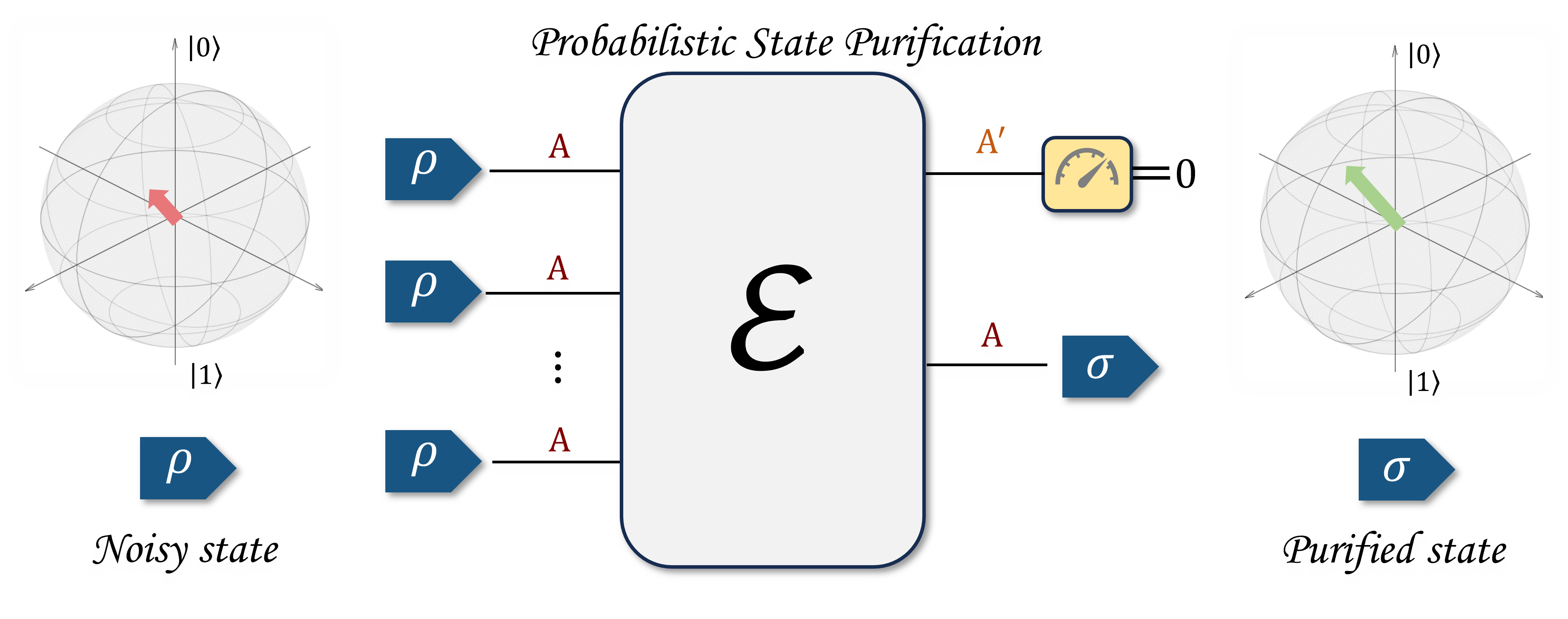
Fig 1: Framework of the purification protocol designed to purify an unknown noisy state $\rho$ into a purer state $\sigma$ by utilizing $n$ copies of the state. The process involves applying a measurement to the system $A^{\prime}$. When the measurement outcome is zero, the protocol successfully yields the purified state $\sigma$; otherwise, we discard it and repeat this purification process.

Notice that probabilistic purification protocols are characterized by two key measures: the average fidelity between the output state of purification protocols and the ideal pure state, and the associated purification probability. Consequently, our investigation focuses on protocols that can achieve the highest average fidelity for a given probability, as well as those that can attain the highest average probability for a given fidelity. To formalize this, we introduce the following definitions.

Definition 1 (Maximal average fidelity for given probability)

Let ${\cal N}$ be the noise channel applied to system $A$ and $n$ be the number of copies of the noisy state. For any given probability $p\in(0,1)$, the maximal average fidelity over all possible protocols is defined as

$$F_{{\cal N}}(n,p)\mathrel{\mathop{\mathchar 58\relax}}=\max\left\{\frac{\int\operatorname{Tr}[\sigma_{\psi}\psi]\,d\psi}{\int\operatorname{Tr}[\sigma_{\psi}]\,d\psi}\Big{\arrowvert}\int\operatorname{Tr}[\sigma_{\psi}]\,d\psi=p,\,{\cal E}_{A^{n}\to A^{\prime}A}\in\rm{CPTN}\right\},$$ (1)

where $\sigma_{\psi}\mathrel{\mathop{\mathchar 58\relax}}=\operatorname{Tr}_{A^{\prime}}[(|0\rangle\!\langle 0|_{A^{\prime}}\otimes I_{A}){\cal E}_{A^{n}\to A^{\prime}A}({\cal N}(\psi)^{\otimes n})(|0\rangle\!\langle 0|_{A^{\prime}}\otimes I_{A})]$, and the integral is taken with respect to the Haar measure over all unit vectors in the Hilbert space ${\cal H}_{A}$.

Similarly, the optimal purification probability is given by the following definition:

Definition 2 (Maximal average probability for given fidelity)

Let ${\cal N}$ be the noise channel applied to system $A$ and $n$ be the number of copies of the noisy state. For any given fidelity $f\in(0,1)$, the maximal average probability over all possible protocols is defined as

$$P_{{\cal N}}(n,f)\mathrel{\mathop{\mathchar 58\relax}}=\max\left\{\int\operatorname{Tr}[\sigma_{\psi}]\,d\psi\Big{\arrowvert}\frac{\int\operatorname{Tr}[\sigma_{\psi}\psi]\,d\psi}{\int\operatorname{Tr}[\sigma_{\psi}]\,d\psi}=f,\,{\cal E}_{A^{n}\to A^{\prime}A}\in\rm{CPTN}\right\},$$ (2)

where $\sigma_{\psi}\mathrel{\mathop{\mathchar 58\relax}}=\operatorname{Tr}_{A^{\prime}}[(|0\rangle\!\langle 0|_{A^{\prime}}\otimes I_{A}){\cal E}_{A^{n}\to A^{\prime}A}({\cal N}(\psi)^{\otimes n})(|0\rangle\!\langle 0|_{A^{\prime}}\otimes I_{A})]$, and the integral is taken with respect to the Haar measure over all unit vectors in the Hilbert space ${\cal H}_{A}$.

We designate a CPTN map as the optimal probabilistic purification protocol for a given purification probability $p$ if it can attain the maximum average fidelity $F_{{\cal N}}(n,p)$. Similarly, if it can achieve the highest average probability $P_{{\cal N}}(n,f)$, we label it as the optimal probabilistic purification protocol for a given purification fidelity $f$. These two measures provide a framework for a detailed exploration of probabilistic purification protocols and trade-offs between purification fidelity and probability.

3.1 Semidefinite programs for purification protocols

In this section, we investigate probabilistic purification protocols using the semidefinite programs (SDP) technology, which can be efficiently solved by the interior point method [BV04] with a runtime polynomial in system dimension $d$. Specifically, we formalize two SDPs to calculate the maximal average fidelity and the probability, respectively. First, we demonstrate the former through the following result:

Proof.

We are going to demonstrate the objective function and the corresponding constraints of the primal SDP, respectively. By definition, we investigate the objective function of the primal SDP as follows:

$$\int\operatorname{Tr}[\sigma_{\psi}\psi]d\psi =\int\operatorname{Tr}[\operatorname{Tr}_{A^{\prime}}[(|0\rangle\!\langle 0|_{A^{\prime}}\otimes I_{A}){\cal E}_{A^{n}\to A^{\prime}A}({\cal N}(\psi)^{\otimes n})(|0\rangle\!\langle 0|_{A^{\prime}}\otimes I_{A})]\psi]d\psi$$ (4)

$$=\int\operatorname{Tr}[\operatorname{Tr}_{A^{n}}[T(J^{\cal E}_{A^{n}A^{\prime}A})({\cal N}(\psi)^{\otimes n}\otimes I_{A^{\prime}A})]|0\rangle\!\langle 0|_{A^{\prime}}\otimes\psi]\,d\psi$$

$$=\int\operatorname{Tr}[T(J^{\cal E}_{A^{n}A^{\prime}A})({\cal N}(\psi)^{\otimes n}\otimes I_{A^{\prime}A})\otimes|0\rangle\!\langle 0|_{A^{\prime}}\otimes\psi]\,d\psi$$

$$=\operatorname{Tr}[J^{{\cal E}}_{{A^{n}A^{\prime}A}}Q^{T}],$$

where $Q\mathrel{\mathop{\mathchar 58\relax}}=\int{\cal N}(\psi)^{\otimes n}\otimes|0\rangle\!\langle 0|_{A^{\prime}}\otimes\psi\,d\psi$ and $T$ denotes partial transpose on system $A^{n}$. Using Schur lemma [Har13, KW20], that is the property, $\Pi_{n}=\tbinom{n+d-1}{n}\int\psi^{\otimes n}\,d\psi$, one can find that $Q={\cal N}^{\otimes n}\circ id(\Pi_{n+1}/D(n+1,d))\otimes|0\rangle\!\langle 0|_{A^{\prime}}$. Similarly, one can conclude that $R\mathrel{\mathop{\mathchar 58\relax}}=\int{\cal N}(\psi)^{\otimes n}\otimes|0\rangle\!\langle 0|_{A^{\prime}}\otimes I_{A}\,d\psi={\cal N}^{\otimes n}(\Pi_{n}/D(n,d))\otimes|0\rangle\!\langle 0|_{A^{\prime}}\otimes I_{A}$. Furthermore, the constraints derive from the fact that ${\cal E}_{A^{n}\to A^{\prime}A}$ is a CPTN map. Therefore, we complete this proof.     $\sqcap$$\sqcup$

We retain the derivation about dual SDP in Appendix A. The primal and dual SDPs proposed in Proposition 1 allow us to characterize the optimal probabilistic purification protocol for a given purification probability. Similarly, we present a similar SDP to calculate the maximal average probability for a fixed purification fidelity.

$$\small\begin{aligned} &\underline{\textbf{Primal Program}}\\ P_{{\cal N}}(n,f)=\max\;&\operatorname{Tr}[J^{{\cal E}}_{{A^{n}A^{\prime}A}}R^{T}]\\ {\rm s.t.}\;&\operatorname{Tr}[J^{{\cal E}}_{{A^{n}A^{\prime}A}}Q^{T}]=\operatorname{Tr}[J^{{\cal E}}_{{A^{n}A^{\prime}A}}R^{T}]f,\\ &J^{{\cal E}}_{A^{n}A^{\prime}A}\geq 0,\,\operatorname{Tr}_{A^{\prime}A}[J_{A^{n}A^{\prime}A}^{{\cal E}}]\leq I_{A^{n}}\end{aligned}\quad\small\begin{aligned} &\underline{\textbf{Dual Program}}\\ \min\;&-\operatorname{Tr}[Y_{A^{n}}]\\ {\rm s.t.}\;&(1-xf)R^{T}+Q^{T}x+\\ &\quad\quad\quad Y_{A^{n}}\otimes I_{A^{\prime}A}\leq 0,\end{aligned}$$ (5)

A derivation can be seen in Appendix A. There is a similar SDP proposed in [Fiu04] which can obtain the maximal average probability for a given maximal average fidelity. However, in this work we have extended this result, that is, the SDP in Eq. (5) allows us to calculate the maximal average probability for any given purification fidelity. This means that one can observe the trend of probability as purification fidelity changes. In summary, the SDPs in Eq. (3) and Eq. (5) facilitate our exploration of the trade-off between the average fidelity and probability.

It is worth emphasizing that the versatility of our SDPs enables them to operate effectively across a wide range of noise channels. Moreover, when focusing on a particular noise channel, their performance becomes even more remarkable. In the subsequent section, we delve into the specifics.

3.2 Purification for depolarizing noise

In this section, we focus on the depolarizing noise, which can describe average noise for large-scale circuits involving many qudits and gates [UNP⁺21]. It is crucial for quantum computation and quantum communication to overcome this noise. Utilizing the SDPs in Eq. (3) and Eq. (5) we investigate the explicit purification protocol, the average fidelity, and the corresponding probability.

Firstly, we are going to show that there exists a purification protocol that can obtain average fidelity $f_{n}$ with probability $p_{n}$, which is the maximal average probability over all protocols that can achieve the fidelity $f_{n}$. Then, we will demonstrate that $f_{n}$ is the maximal fidelity for all given probabilities. In specific, we have the following result:

Proof.

First, we are going to show $f_{n}\leq F_{Depo}(n,p_{n})$ using the primal SDP in Eq. (3). Specifically, it is straightforward to see that the following Choi operator is a feasible solution:

$$J^{{\cal E}}_{A^{n}A^{\prime}A}\mathrel{\mathop{\mathchar 58\relax}}=|0\rangle\!\langle 0|_{A^{\prime}}\otimes\operatorname{Tr}_{n-1}[J^{{\cal M}_{n}}_{A^{n}A^{n}}],$$ (7)

where $J^{{\cal M}_{n}}_{A^{n}A^{n}}$ denotes the Choi operator of ${\cal M}_{n}(\cdot)$, ${\cal M}_{n}(\cdot)\mathrel{\mathop{\mathchar 58\relax}}=\Pi_{n}(\cdot)\Pi^{\dagger}_{n}$ and $\Pi_{n}$ is the projector on the symmetric subspace of ${\cal H}^{\otimes n}_{A}$, and $\operatorname{Tr}_{n-1}[\cdot]$ denotes the partial trace on the last $n-1$ subsystems. Then, we demonstrate that one can obtain the objective value $f_{n}$ using this solution, as follows:

$$\operatorname{Tr}[J^{{\cal E}}_{A^{n}A^{\prime}A}Q^{T}] =\operatorname{Tr}[T(J^{{\cal E}}_{A^{n}A^{\prime}A}){\cal N}^{\otimes n}\circ id(\Pi_{n+1}/D(n+1,d))\otimes|0\rangle\!\langle 0|_{A^{\prime}}]$$ (8)

$$=\int\operatorname{Tr}[T(J^{{\cal E}}_{A^{n}A^{\prime}A}){\cal N}(\psi)^{\otimes n}\otimes|0\rangle\!\langle 0|_{A^{\prime}}\otimes\psi]\,d\psi$$

$$=\int\operatorname{Tr}[\psi\operatorname{Tr}_{A^{n}A^{\prime}}[T(J^{{\cal E}}_{A^{n}A^{\prime}A}){\cal N}(\psi)^{\otimes n}\otimes|0\rangle\!\langle 0|_{A^{\prime}}\otimes I_{A}]]\,d\psi$$

$$=\int\operatorname{Tr}[\psi\operatorname{Tr}_{n-1}[\Pi_{n}{\cal N}(\psi)^{\otimes n}\Pi_{n}^{\dagger}]]\,d\psi$$

$$=\langle 0|\operatorname{Tr}_{n-1}[\Pi_{n}\Lambda^{\otimes n}\Pi_{n}^{\dagger}]|0\rangle$$

where the fifth equation follows from the fact that $\langle 0|\operatorname{Tr}_{n-1}[\Pi_{n}\Lambda^{\otimes n}\Pi_{n}^{\dagger}]|0\rangle=\langle\psi|\operatorname{Tr}_{n-1}[\Pi_{n}{\cal N}(\psi)^{\otimes n}\Pi_{n}^{\dagger}]|\psi\rangle$ for any pure state $\psi$. Furthermore, we have $\operatorname{Tr}[J^{{\cal E}}_{A^{n}A^{\prime}A}R^{T}]=\operatorname{Tr}[\Pi_{n}\Lambda^{\otimes n}]$ in the same way. According to Lemma S2, we further obtain the recursive forms of probability and fidelity, which means $F_{Depo}(n,p)\geq f_{n}$.

Second, we demonstrate that $\{-f_{n},\mathbf{0}\}$ is a feasible solution of the dual SDP in Eq. (3). Specifically, we observe the constraint as follows:

$$f_{n}R^{T}-Q^{T} =\int T({\cal N}(\psi)^{\otimes n})\otimes|0\rangle\!\langle 0|_{A^{\prime}}\otimes(f_{n}I_{A}-\psi)\,d\psi$$ (9)

$$=\int(U^{\ast\otimes n}\otimes I_{A^{\prime}}\otimes U)\Lambda^{\otimes n}\otimes|0\rangle\!\langle 0|_{A^{\prime}}\otimes(f_{n}I_{A}-\Lambda)(U^{T\otimes n}\otimes I_{A^{\prime}}\otimes U^{\dagger})\,dU\geq 0,$$

where the second equation holds because the depolarizing channel ${\cal N}$ commutes with unitary operations, and the inequality is derived from the fact that $f_{n}I_{A}-\Lambda\geq 0$. These imply $F_{Depo}(n,p_{n})\leq f_{n}$. Combining the primal part and the dual part, we conclusively establish that $F_{Depo}(n,p_{n})=f_{n}$.

Similarly, one can find that the $J^{{\cal E}}_{A^{n}A^{\prime}A}$ and $\{+\infty,-\Pi_{n}p_{n}/D(n,d)\}$ are the feasible solutions of the primal and dual SDP in Eq. (5) for calculating $P_{Depo}(n,f_{n})$, respectively, where $D(n,d)\mathrel{\mathop{\mathchar 58\relax}}=\tbinom{n+d-1}{n}$. Notably, for a sufficiently large $x$, the following inequality is satisfied:

$$(1-xf_{n})R^{T}+Q^{T}x+Y_{A^{n}}\otimes I_{A^{\prime}A}\leq 0,$$ (10)

which is equivalent to $f_{n}R^{T}-Q^{T}\geq 0$. Similarly, combining the primal part and the dual part, we have $P_{Depo}(n,f_{n})=p_{n}$. Thus, we complete the proof.     $\sqcap$$\sqcup$

A natural issue is whether there exists a purification probability $p$ such that the optimal purification protocol can obtain higher fidelity, i.e., $F_{Depo}(n,p)\geq f_{n}$. We answer this question using the following conclusion:

Proof.

First, we are going to show the purification fidelity $F_{Depo}(n,p)$ is a decreasing function with respect to the purification probability $p\in(0,1)$, i.e., $F_{Depo}(n,p)\geq F_{Depo}(n,q)$ for $p\leq q\in(0,1)$. Specifically, let $J_{q}$ be the optimal solution of the primal SDP in Eq. (3) for fixing purification probability $q$, that is, $F_{Depo}(n,q)=\operatorname{Tr}[J_{q}Q]/q$. Then, the Choi operator $J_{p}\mathrel{\mathop{\mathchar 58\relax}}=\frac{p}{q}J_{q}$ is a feasible solution of the primal SDP in Eq. (3) for fixing purification probability $p$, which means

$$F_{Depo}(n,p)\geq\operatorname{Tr}[J_{p}Q]/p=\operatorname{Tr}[J_{q}Q]/q=F_{Depo}(n,q).$$ (12)

Second, we demonstrate that even if the purification probability is reduced, it will not increase the purification fidelity, that is, $F_{Depo}(n,p)=f_{n}$ for all $p\leq p_{n}$. In specific, one can check that the Choi operator $J_{p}\mathrel{\mathop{\mathchar 58\relax}}=\frac{p}{p_{n}}J^{{\cal E}}_{A^{n}A^{\prime}A}$ is the optimal solution of the primal SDP in Eq. (3) with respects to probability $p$, where the definition of $J^{{\cal E}}_{A^{n}A^{\prime}A}$ is proposed in the proof of Theorem 2. Therefore, we obtain that $f_{n}$ is the maximal purification fidelity for all given probabilities.     $\sqcap$$\sqcup$

Remark 1 (Optimal purification protocol) Theorem 2 and Proposition 3 demonstrate that the optimal probabilistic purification protocol both for given fidelity and probability is given by

$${\cal E}^{\ast}_{A^{n}\to A^{\prime}A}\mathrel{\mathop{\mathchar 58\relax}}={\cal R}_{0}\circ\operatorname{Tr}_{n-1}\circ{\cal M}_{n},$$ (13)

where ${\cal R}_{0}(\cdot)\mathrel{\mathop{\mathchar 58\relax}}=|0\rangle\!\langle 0|_{A^{\prime}}\otimes(\cdot)$ denotes the replacement channel, $\operatorname{Tr}_{n-1}[\cdot]$ denotes the partial trace on the last $n-1$ subsystems $A^{n-1}$, ${\cal M}_{n}(\cdot)\mathrel{\mathop{\mathchar 58\relax}}=\Pi_{n}(\cdot)\Pi^{\dagger}_{n}$ and $\Pi_{n}$ is the projector on the symmetric subspace of ${\cal H}^{\otimes n}_{A}$. For depolarizing noise, the protocol can obtain the maximal average fidelity $f_{n}$ with probability $p_{n}$ which is also maximal for all protocols that can achieve this maximal fidelity $f_{n}$, which is shown in Fig. 2.

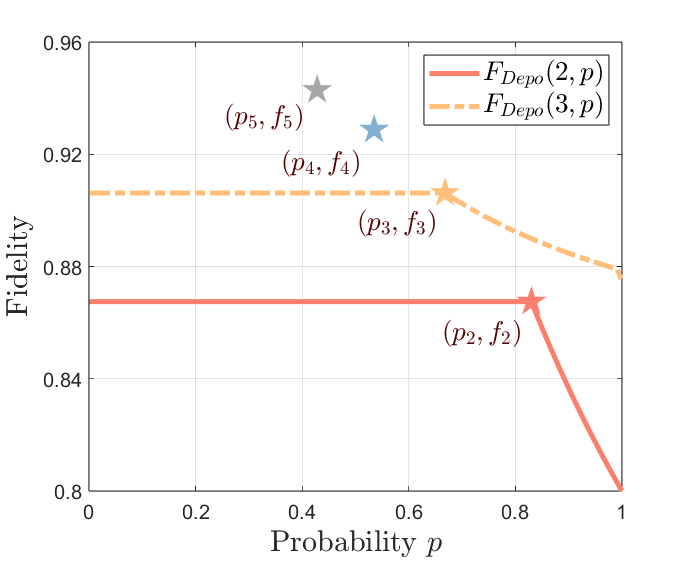
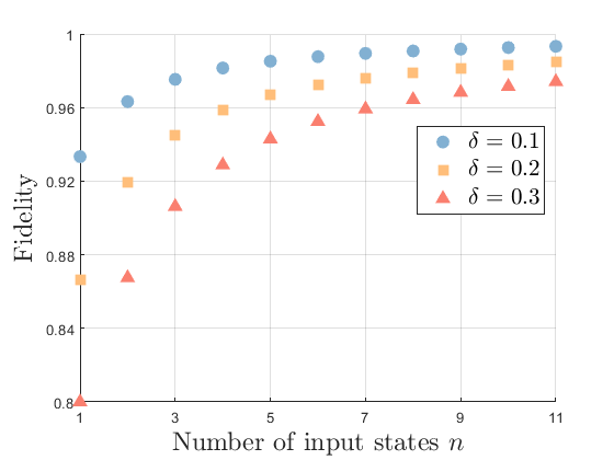
Fig 2: Average purification fidelity $F_{\text{Depo}}(n,p)$ with different number of input depolarized states $n$ and average success probability $p$. (a) describes the relationship between the optimal protocol ${\cal E}^{\ast}_{A^{n}\to A^{\prime}A}$ proposed in Remark 3.2 and the protocols obtained from the SDP in Eq.(3) when the error parameter $\delta$ is $0.3$ and the dimension $d=3$. The star-markers obtained by the optimal protocol ${\cal E}^{\ast}_{A^{n}\to A^{\prime}A}$ follow from the probability $p_{n}\mathrel{\mathop{\mathchar 58\relax}}=\frac{1}{n}\sum_{j=1}^{n}p_{n-j}\operatorname{Tr}\left[\Lambda^{j}\right]$ and fidelity $f_{n}\mathrel{\mathop{\mathchar 58\relax}}=\frac{1}{n}\sum_{j=1}^{n}p_{n-j}\lambda_{0}^{j}/p_{n}$, respectively. (b) describes the trend of the maximal average fidelity $f_{n}$ with $n$ for different noise parameters $\delta$.

It is worth noting that the authors made a similar observation in  [Fiu04]. However, we demonstrate it differently and propose more explicit forms encompassing the purification protocol, fidelity, and probability. In specific, from Fig. 2, one can observe that the probabilistic purification protocols involve a trade-off between fidelity and probability, and there is an inflection point where the average fidelity is highest and the fidelity will decrease after this point, which we call the golden point for probabilistic purification. Remarkably, for depolarizing noise, there exists an explicit protocol that can achieve this golden point. Furthermore, one can calculate the maximal fidelity $f_{n}$ and the corresponding probability $p_{n}$ directly depending on their recursive forms instead of solving SDPs, which means we can analyze the trade-off between fidelity and probability in cases where $n$ is large. In addition, Fig. 2 depicts the trend that the maximal average fidelity $f_{n}$ will converge to one as the number of input state $n$ increases for different error parameters.

3.3 Purification circuits based on block encoding

In this section, we investigate the circuit implementation of the optimal probabilistic purification protocol for depolarizing noise ${\cal E}^{\ast}_{A^{n}\to A^{\prime}A}$ using the block encoding technique [LC19, GSLW19, CLVBY22]. Observe that for any input depolarizing noisy state $\rho^{\otimes n}$, we have ${\cal E}^{\ast}_{A^{n}\to A^{\prime}A}(\rho^{\otimes n})=|0\rangle\!\langle 0|\otimes\operatorname{Tr}_{n-1}[\Pi_{n}\rho^{\otimes n}\Pi_{n}]=\operatorname{Tr}_{n-1}[(|0\rangle\!\langle 0|\otimes\Pi_{n})(|0\rangle\!\langle 0|\otimes\rho^{\otimes n})(|0\rangle\!\langle 0|\otimes\Pi_{n})]$. It means that the implementation task is equivalent to block encode the symmetric projector $\Pi_{n}$, i.e., constructing a quantum circuit $U$, such that

$$\begin{aligned} U=\left[\begin{array}[]{cc}\Pi_{n}&\cdot\\ \cdot&\cdot\end{array}\right]\end{aligned},$$ (14)

where $\Pi_{n}$ is the projector on the symmetric subspace of ${\cal H}^{\otimes n}_{A}$. Notice that by definition, the projector $\Pi_{n}$ is a linear combination of unitaries, i.e., $\Pi_{n}=\sum_{c\in{\cal S}_{n}}\frac{1}{n!}\mathbf{P}_{n}(c)$, where $\mathbf{P}_{n}(c)$ is the permutation operator of the symmetric group ${\cal S}_{n}$ of degree $n$. Thus, one can block encode this projector $\Pi_{n}$ by the linear combinations of unitaries (LCU) algorithm [CW12, LKWI23]. It consists of the preparation circuit and selection circuit. The former can produce a superposition state determined by coefficients of unitaries, while the latter functions to choose the corresponding unitary based on control qudits. Specifically, we present the following result to demonstrate how to implement the optimal probabilistic purification protocol ${\cal E}^{\ast}_{A^{n}\to A^{\prime}A}$ using a quantum circuit.

Proposition 4 implies that for a given $d$-dimensional depolarized state $\rho^{\otimes n}$ one can reconstruct a state $\sigma$ with high purity by employing a specific quantum circuit. For the sake of simplicity, we illustrate the circuit implementation method in this case when considering $n=3$ and $d=2$. The specific circuit is shown in Fig. 3. In addition, one can find that if $n=2$, the purification circuit can be reduced to the swap test gadget proposed in [CFL⁺23].

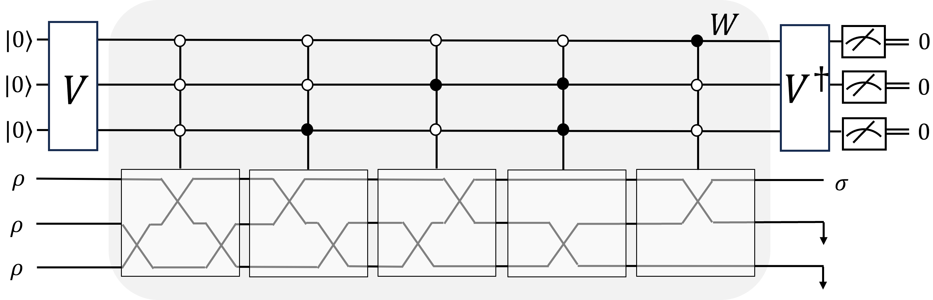
Fig 3: The purification circuit for three input noisy qubit states. The preparation circuit $V$ satisfies $V|0\rangle=\sum_{j=0}^{5}\frac{1}{\sqrt{6}}|j\rangle$, and the selection circuit $W$ consists of five different controlled-$\mathbf{P}_{3}(c)$ gates, where $c\in\{(1,2),(1,3),(2,3),(1,2,3),(1,3,2)\}$.

Noticing that the purification circuit proposed in Proposition 4 involves $\lceil\log_{d}(n!-1)\rceil$ controlled qudits, which hinders its application in practice. Therefore, we further investigate reducing the use of controlled qudits by employing rotation gates rather than the selection circuit and using the properties of permutation operators of the symmetric group. Specifically, for the circuit shown in Fig. 3, we present a simplified form as follows:

Proof.

Observing that for any quantum state $\rho\in{\cal D}({\cal H}_{A})$ we have ${\cal E}^{\ast}_{A^{3}\to A^{\prime}A}(\rho^{\otimes 3})=\operatorname{Tr}_{2}[(|0\rangle\!\langle 0|\otimes\Pi_{3})(|0\rangle\!\langle 0|\otimes\rho^{\otimes 3})(|0\rangle\!\langle 0|\otimes\Pi^{\dagger}_{3})]$, which means we only need to construct a quantum circuit which is block-encoded by the projector $\Pi_{3}$. Specifically, we are going to show $(\langle 0|\otimes I_{3})U_{3\to 1}(|0\rangle\otimes I_{3})=\Pi_{3}$. Notice that

$$(\langle 0|\otimes I_{3})U_{3\to 1}(|0\rangle\otimes I_{3}) =\langle 0|R_{y}(\gamma)|0\rangle\langle 0|R_{y}(\beta)|0\rangle\langle 0|R_{y}(\alpha)|0\rangle I_{3}$$ (17)

$$\quad+\langle 0|R_{y}(\gamma)|0\rangle\langle 0|R_{y}(\beta)|1\rangle\langle 1|R_{y}(\alpha)|0\rangle\mathbf{P}_{3}((1,2,3))$$

$$\quad+\langle 0|R_{y}(\gamma)|1\rangle\langle 1|R_{y}(\beta)|0\rangle\langle 0|R_{y}(\alpha)|0\rangle\mathbf{P}_{3}((1,3,2))$$

$$\quad+\langle 0|R_{y}(\gamma)|1\rangle\langle 1|R_{y}(\beta)|1\rangle\langle 1|R_{y}(\alpha)|0\rangle\mathbf{P}_{3}((1,3,2))\mathbf{P}_{3}((1,2,3)),$$

and permutation operators of the symmetry group ${\cal S}_{3}$ satisfy $\mathbf{P}_{3}((1,2))+\mathbf{P}_{3}((1,3))+\mathbf{P}_{3}((2,3))=\mathbf{P}_{3}((1))+\mathbf{P}_{3}((1,2,3))+\mathbf{P}_{3}((1,3,2))$, which implies that the projector on the symmetric subspace ${\cal H}^{\otimes 3}_{A}$ can be rewritten as $\Pi_{3}=\frac{1}{3}\left[\mathbf{P}_{3}((1))+\mathbf{P}_{3}((1,2,3))+\mathbf{P}_{3}((1,3,2))\right]$, and $\mathbf{P}_{3}((1,2,3))\mathbf{P}_{3}((1,3,2))=\mathbf{P}_{3}((1))$. It is straightforward to check that one can set $\alpha=\gamma=-\arctan(\sqrt{2})$ and $\beta=\arccos(-1/3)$ such that Eq. (17) equals to $\Pi_{3}$, which completes this proof. The specific circuit is shown in Fig. 4.     $\sqcap$$\sqcup$

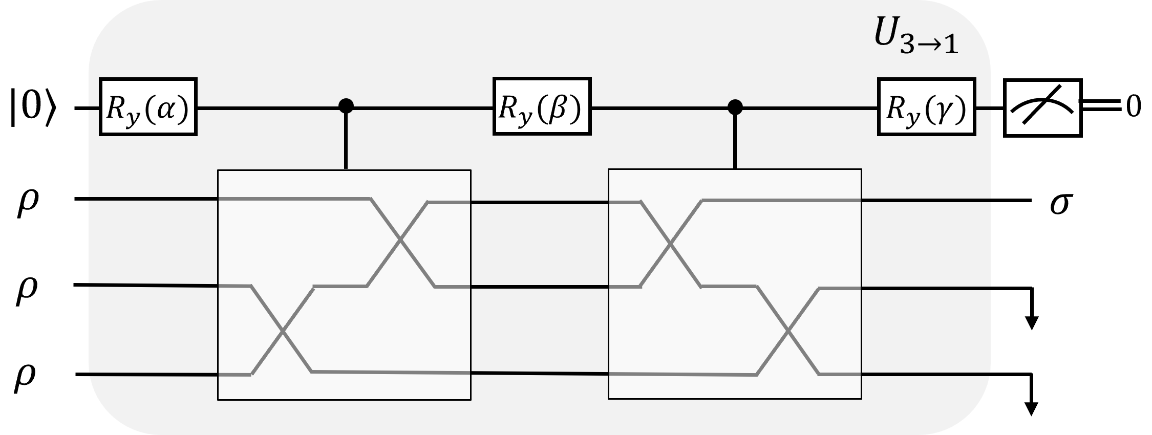
Fig 4: The simplified purification circuit for given three input noisy qubit states. We set the rotation parameters $\alpha=\gamma=-\arctan(\sqrt{2})$ and $\beta=\arccos(-1/3)$, and apply measurement on the auxiliary system $A^{\prime}$. Then, we obtain the purified state $\sigma$ if the measurement outcome is zero.

The purification circuit depicted in Fig. 4 is relatively simple to implement. With any input noisy state $\rho^{\otimes 3}$, this protocol allows us to generate an output state $\sigma$ that exhibits high fidelity with the ideal pure state $|\psi\rangle$. Specifically, the output state $\sigma$ can rewritten as the following form:

$$\sigma=\frac{\frac{1}{3}\rho+\frac{2}{3}\rho^{3}}{\frac{1}{3}+\frac{2}{3}\operatorname{Tr}[\rho^{3}]}=(1-\delta^{\prime})|\psi\rangle\!\langle\psi|+\delta^{\prime}\frac{I}{2},\quad\delta^{\prime}\mathrel{\mathop{\mathchar 58\relax}}=\frac{2\delta+\delta^{3}}{6p(\delta)},$$ (18)

where $p(\delta)\mathrel{\mathop{\mathchar 58\relax}}=1-\delta+\frac{1}{2}\delta^{2}$ represents the probability of obtaining the measurement outcome zero, i.e., the purification probability. This purification circuit can be treated as a gadget and can be utilized to construct a recursive purification protocol. Further analysis of stream purification can be done via the technique in Ref. [CFL⁺23].

4 Extensions and Examples

In this section, we benchmark the performance of the probabilistic purification protocols obtained by SDPs. In specific, in Sec. 4.1, we present the estimation of sample complexity of the optimal protocol ${\cal E}^{\ast}_{A^{n}\to A^{\prime}A}$ for the depolarizing noise. In addition, we propose a general recursive purification protocol and depict the relationship between the maximal average fidelity and recursive depth. We also show the efficiency of SDP in searching purification protocols for other noises, including Pauli noise [EWP⁺19], dephasing noise [AMM20], and amplitude damping noise [NC01] in Sec. 4.3.

4.1 Sample complexity estimation

As the optimal purification protocol ${\cal E}^{\ast}_{A^{n}\to A^{\prime}A}$ is probabilistic, we are interested in the expected number of depolarized states consumed in this protocol, also known as the sample complexity. To estimate the sample complexity, we introduce a classical algorithm based on the recursive forms of maximal fidelity $f_{n}$ and probability $p_{n}$ proposed in Theorem 2. The algorithm is designed to handle an input error parameter $\delta$, system dimension $d$, the desired output fidelity $f_{goal}$, and return the number of input states $n$ during this protocol and the expected number of noisy states $\frac{n}{p_{n}}$. By utilizing Alg. 1, one can determine the expected numbers of noisy states consumed in the probabilistic protocol ${\cal E}^{\ast}_{A^{n}\to A^{\prime}A}$ for any target fidelity $f_{goal}\in(0,1)$ and system dimension $d\geq 2$. The scaling of the sample complexity is presented in Table 2.

1

input : Goal fidelity $f_{goal}$, error parameter $\delta$ for depolarizing noise and dimension $d$ of Hilbert spaces ${\cal H}_{A}$

2

output : The number of input noisy states and the expected number of noisy states consumed during this protocol

3 $n\leftarrow 0$, $p_{0}\leftarrow 1$ and $\Lambda\mathrel{\mathop{\mathchar 58\relax}}=\operatorname{Diag}(\lambda_{0}\,\cdots,\lambda_{d-1})$

4$\lambda_{0}\leftarrow 1-\frac{d-1}{d}\delta$, $\lambda_{j\neq 0}\leftarrow\frac{\delta}{d}$

5 repeat

6      Number of input noisy states $n\leftarrow n+1$

7       $n_{th}$ success probability $p_{n}\leftarrow\frac{1}{n}\sum_{j=1}^{n}p_{n-j}\operatorname{Tr}\left[\Lambda^{j}\right]$

8       $n_{th}$ output fidelity $f_{n}\leftarrow\frac{1}{n}\sum_{j=1}^{n}p_{n-j}\lambda_{0}^{j}/p_{n}$

9until $f_{n}\geq f_{goal}$;

return $n$, $\frac{n}{p_{n}}$

Algorithm 1 Estimation of Sample Complexity

$f_{goal}$	$0.9285$	$0.9682$	$0.9801$	$0.9842$	$0.9880$	$0.9894$	$0.9900$
${n}$	$3$	$8$	$14$	$18$	$23$	$26$	$28$
$\frac{n}{p_{n}}$	$8$	$5.2\times 10^{1}$	$3.27\times 10^{2}$	$1.01\times 10^{3}$	$3.89\times 10^{3}$	$8.55\times 10^{3}$	$1.43\times 10^{4}$

Table 2: Estimation of sample complexity. $f_{goal}$ denotes the target fidelity, $n$ is the number of the input noisy state, and $\frac{n}{p_{n}}$ is the expected numbers of depolarized states $\rho$ with error parameter $\delta=0.3$ and dimension $d=3$.

4.2 Recursive purification

Moreover, it is natural to consider this protocol as a foundational element for constructing a recursive purification procedure aimed at enhancing fidelity as the recursive depth increases. Specifically, we propose a general recursive purification method as follows:

1

input : The number of the noise qudit $\rho$ consumed per recursion $n$, and the recursive depth $m$

output : Purified state $\sigma_{n,m}$

2

3if m=0 then

4       return $\sigma_{n,0}\leftarrow\rho$

5      

6else

7       $\sigma_{n,m-1}\leftarrow$GR-PURIFY$(n,m-1)$

8       repeat

9            Apply the purification circuit mentioned in Proposition 4 to $\sigma_{n,m-1}$ and denote the measurement outcome by $a$.

10      until a = 0;

11      return Purified state $\sigma_{n,m}$

12 end if

Algorithm 2 General Recursive Purification, named GR-PURIFY$(n,m)$

It is important to note that in [CFL⁺23], the authors introduced a recursive purification protocol based on the swap test procedure, which corresponds to the case of $n=2$ in our protocol. However, a significant challenge for quantum memory arises as some purified states must be maintained with long coherence in this recursive protocol as the depth increases. As depicted in Fig. 5, it is evident that the general recursive purification protocol proposed in Alg. 2 requires a lower recursive depth to achieve the same target fidelity compared to the recursive purification procedure based on the swap test.

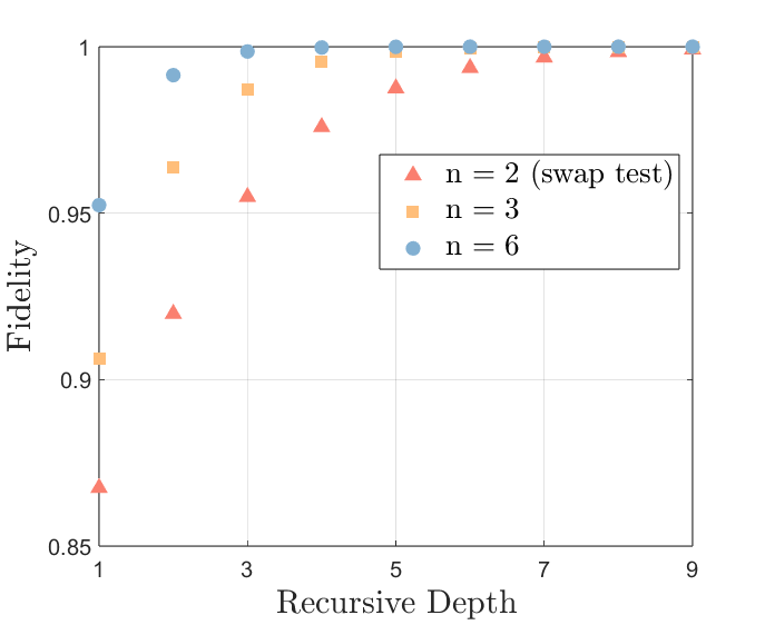
Fig 5: Trend of fidelity between output state $\sigma_{n,m}$ presented in Alg. 2 and the corresponding ideal state as recursive depth increases. The error parameter of depolarizing noise $\delta=0.3$ and the dimension of noisy states $d=3$.

4.3 Purification for different noises

In this section, we focus on the comparison between the protocols obtained by SDPs and the protocol based on the swap test for different types of noise in Fig. 6.

Without loss of generality, we consider the cases in which two and three copies of the noisy state are consumed in the purification protocols, i.e., the case of $n=2$ and $n=3$, respectively. Specifically, we denote $I$, $X$, $Y$ and $Z$ as Pauli operators on qubit systems, and $\delta$ as the error parameter for different noise channels, including the Pauli noise with Kraus operators $K_{0}\mathrel{\mathop{\mathchar 58\relax}}=\sqrt{1-0.75\delta}I$, $K_{1}\mathrel{\mathop{\mathchar 58\relax}}=\sqrt{0.1\delta}X$, $K_{2}\mathrel{\mathop{\mathchar 58\relax}}=\sqrt{0.2\delta}Y$, and $K_{3}\mathrel{\mathop{\mathchar 58\relax}}=\sqrt{0.45\delta}Z$ and the amplitude damping noise with Kraus operators $K_{0}\mathrel{\mathop{\mathchar 58\relax}}=|0\rangle\!\langle 0|+\sqrt{1-\delta}|1\rangle\!\langle 1|$ and $K_{1}\mathrel{\mathop{\mathchar 58\relax}}=\sqrt{\delta}|0\rangle\!\langle 1|$. Notice that for the case of $n=3$, the recursive purification protocols based on the swap test procedure can be run by setting the recursive depth equal to two [CFL⁺23].

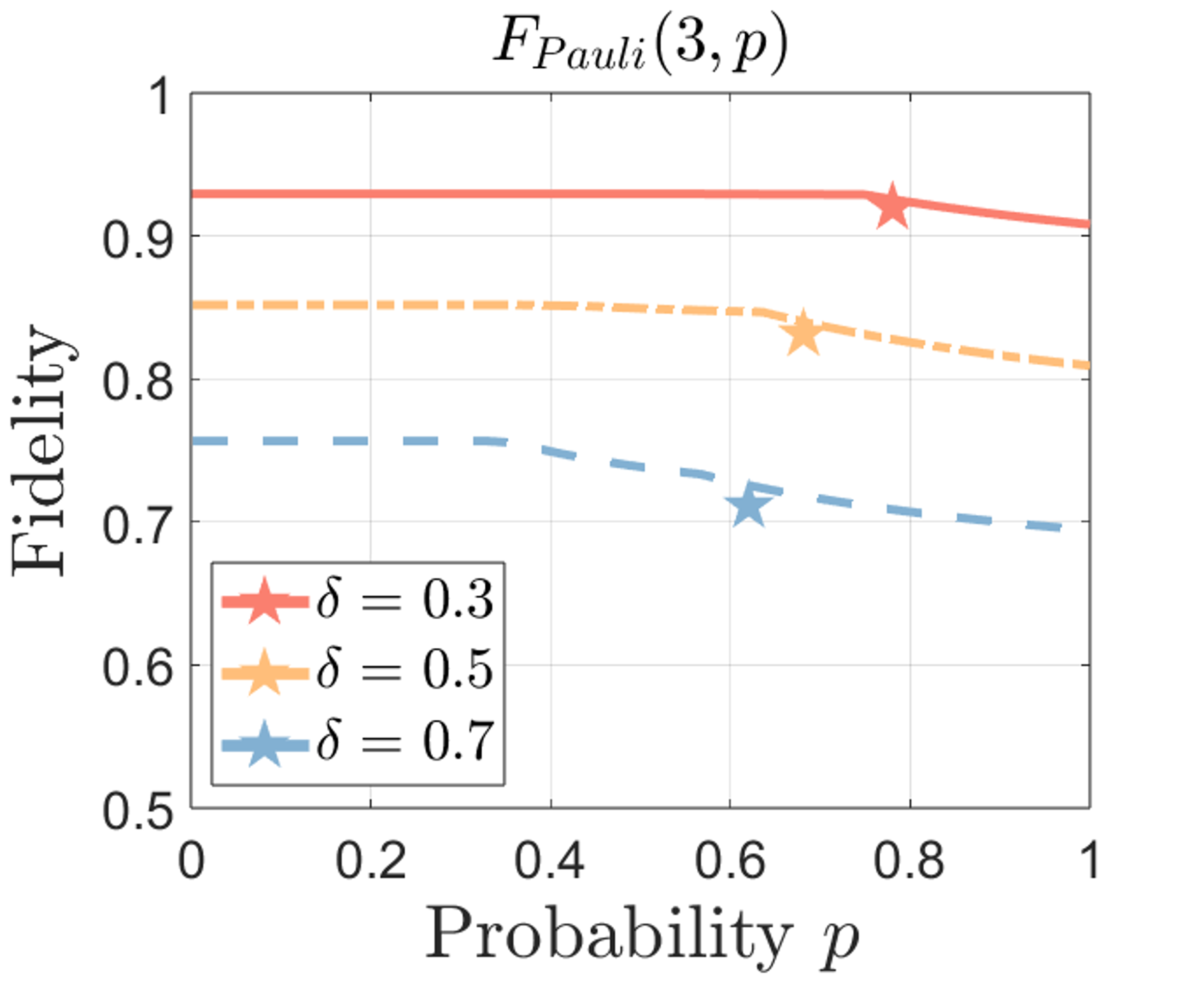
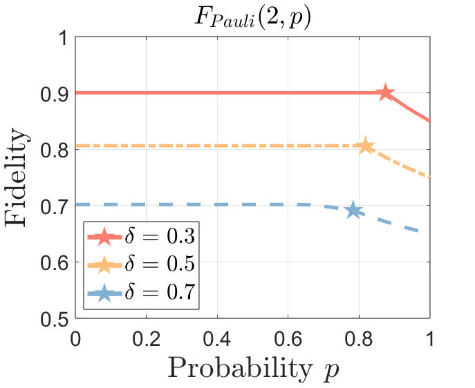
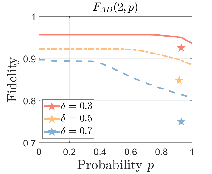
Fig 6: Comparison of purification protocols obtained by SDP and the protocol based on the swap test for different noise channels. The lines describe the relationship between the success probability $p$ and the corresponding fidelity obtained by SDP in Eq. (3). The star-markers describe the results obtained by the protocol based on the swap test. For the Pauli noise, (a) and (b) describe these comparisons with $n=2$ and $n=3$, respectively. (c) describes the comparison for the amplitude damping noise.

In Fig. 6 and Fig. 6, one can see that the results obtained by the swap test method approach the point of the maximal fidelity and high probability obtained by the SDP in Eq. (3) for the case of Pauli noise, especially the error parameters $\delta$ with the small value. The reason is that the depolarizing noise is a special case of the Pauli noise. Note that the patterns of lines and points in the graphs consistently exhibit analogous characteristics as the number of copies $n$ increases. Conversely, the amplitude damping noise is completely different. We find a large gap between the fidelity based on different purification protocols in Fig. 6, which means that compared with the swap test method, the purification protocol obtained by the SDP method carries a significant improvement.

Observing that all star-markers do not stand at the point of the maximal fidelity and high probability in Fiq. 6, especially for the amplitude damping noise. This implies that SDP in Eq. (3) could be useful to explore the optimal probabilistic purification protocols for general noise channels.

5 Conclusions

In this paper, we focus on the state purification task. The implementable protocols via quantum circuits and the involved trade-offs have been investigated. We have presented a general framework for probabilistic state purification. Our approach involves formulating semidefinite programs to compute both the purification fidelity and the corresponding probability. Remarkably, for the case of depolarizing noise, we have proposed an explicit purification protocol that can achieve the golden point $(p_{n},f_{n})$ for purifying $n$-copy noisy states, i.e., the fidelity $f_{n}$ is maximal and the probability $p_{n}$ is also the highest for all protocols that can reach the fidelity $f_{n}$. Meanwhile, we establish the explicit forms of $f_{n}$ and $p_{n}$ to characterize the trade-off between fidelity and probability, especially with the number of input state $n$ increases. More importantly, this protocol has a circuit implementation grounded in block encoding technology, which is also a more flexible and general extension of the Swap Test-based method. Furthermore, we have introduced a recursive purification protocol and analyzed the sample complexities, which demonstrates the flexibility and efficiency compared with the previous stream protocol [CFL⁺23]. We have shown that our recursive protocol involves lower recursive depth than the protocol based on the swap test procedure for given target fidelity, which alleviates the pressure of quantum memory. We have further demonstrated the advantage of our methods in quantum state purification for general noise channels beyond the specific depolarizing noise.

For future work, it will be meaningful to explore how to simplify the purification circuit to reduce the number of controlled qudits, thereby enhancing practical applicability. Another interesting direction is to analyze the optimal probabilistic purification protocol for various noise channels through the SDP characterizations and explore the properties of different noises. It will also be interesting to further extend or apply the techniques of this work to quantum error mitigation (e.g., virtual state purification [Koc21, HMO⁺21, LZFC24]) and to the many purification tasks in quantum resource theories [CG19].

Appendix for
Protocols and Trade-Offs of Quantum State Purification

Appendix A Dual SDP for purification protocols

For a given purification success probability $p$ and number of input state copies $n$, The primal SDP for calculating the optimal purification fidelity $F_{{\cal N}}(n,p)$ is written as follows:

$$F_{{\cal N}}(n,p)=\max \operatorname{Tr}[J^{{\cal E}}_{{A^{n}A^{\prime}A}}Q^{T}]/p$$ (19)

$${\rm s.t.} \operatorname{Tr}[J^{{\cal E}}_{{A^{n}A^{\prime}A}}R^{T}]=p,$$

$$J^{{\cal E}}_{A^{n}A^{\prime}A}\geq 0,\,\operatorname{Tr}_{A^{\prime}A}[J_{A^{n}A^{\prime}A}]\leq I_{A^{n}},$$

where $T$ denotes partial transpose on system $A^{n}$ and

$$Q\mathrel{\mathop{\mathchar 58\relax}}=\int{\cal N}(\psi)^{\otimes n}\otimes|0\rangle\!\langle 0|_{A^{\prime}}\otimes\psi\,d\psi,\quad R\mathrel{\mathop{\mathchar 58\relax}}=\int{\cal N}(\psi)^{\otimes n}\otimes|0\rangle\!\langle 0|_{A^{\prime}}\otimes I_{A}\,d\psi.$$ (20)

Now, we derive its dual SDP. Based on the primal SDP, the Lagrange function can be written as

$$\mathcal{L}(x,Y_{A^{n}},J)\mathrel{\mathop{\mathchar 58\relax}} =\frac{1}{p}\operatorname{Tr}[JQ^{T}]+\langle x,\operatorname{Tr}[JR^{T}]-p\rangle+\langle Y_{A^{n}},\operatorname{Tr}_{A^{\prime}A}[J]-I_{A^{n}}\rangle$$ (21)

$$=-px-\operatorname{Tr}[Y_{A^{n}}]+\langle J,\frac{1}{p}Q^{T}+R^{T}x+Y_{A^{n}}\otimes I_{A^{\prime}A}\rangle,$$ (22)

where $x$, $Y_{A^{n}}$ are Lagrange multipliers. Then, the Lagrange dual function can be written as

$$\mathcal{G}(x, Y_{A^{n}})\mathrel{\mathop{\mathchar 58\relax}}=\sup_{J\geq 0}\mathcal{L}(x,Y_{A^{n}},J).$$ (23)

Since $J^{{\cal N}}\geq 0$, it holds that

$$\frac{1}{p}Q^{T}+R^{T}x+Y_{A^{n}}\otimes I_{A^{\prime}A}\leq 0$$ (24)

otherwise, the inner norm is unbounded. Redefine $x$ as $x/p$ and $Y_{A^{n}}$ as $Y_{A^{n}}/p$. Then, we obtain the following dual SDP.

$$\min -x-\operatorname{Tr}[Y_{A^{n}}]/p$$ (25)

$${\rm s.t.} Q^{T}+R^{T}x+Y_{A^{n}}\otimes I_{A^{\prime}A}\leq 0,$$

It is worth noting that the strong duality is held by Slater’s condition.

Similarly, the primal SDP for calculating the optimal purification success probability $P_{{\cal N}}(n,f)$ is written as follows:

$$P_{{\cal N}}(n,f)=\max \operatorname{Tr}[J^{{\cal E}}_{{A^{n}A^{\prime}A}}R^{T}]$$ (26)

$${\rm s.t.} \operatorname{Tr}[J^{{\cal E}}_{{A^{n}A^{\prime}A}}Q^{T}]=\operatorname{Tr}[J^{{\cal E}}_{{A^{n}A^{\prime}A}}R^{T}]f,$$

$$J^{{\cal E}}_{A^{n}A^{\prime}A}\geq 0,\,\operatorname{Tr}_{A^{\prime}A}[J_{A^{n}A^{\prime}A}]\leq I_{A^{n}}.$$

Now, we derive its dual SDP. Based on the primal SDP, the Lagrange function can be written as

$$\mathcal{L}(x,Y_{A^{n}},J)\mathrel{\mathop{\mathchar 58\relax}} =\operatorname{Tr}[JR^{T}]+\langle x,\operatorname{Tr}[JQ^{T}]-\operatorname{Tr}[JR^{T}]f\rangle+\langle Y_{A^{n}},\operatorname{Tr}_{A^{\prime}A}[J]-I_{A^{n}}\rangle$$ (27)

$$=-\operatorname{Tr}[Y_{A^{n}}]+\langle J,(1-xf)R^{T}+Q^{T}x+Y_{A^{n}}\otimes I_{A^{\prime}A}\rangle,$$ (28)

where $x$, $Y_{A^{n}}$ are Lagrange multipliers. Then, the Lagrange dual function can be written as

$$\mathcal{G}(x, Y_{A^{n}})\mathrel{\mathop{\mathchar 58\relax}}=\sup_{J\geq 0}\mathcal{L}(x,Y_{A^{n}},J).$$ (29)

Since $J^{{\cal N}}\geq 0$, it holds that

$$(1-xf)R^{T}+Q^{T}x+Y_{A^{n}}\otimes I_{A^{\prime}A}\leq 0$$ (30)

otherwise, the inner norm is unbounded. Redefine $x$ as $x/p$ and $Y_{A^{n}}$ as $Y_{A^{n}}/p$. Then, we obtain the following dual SDP.

$$\min -\operatorname{Tr}[Y_{A^{n}}]$$ (31)

$${\rm s.t.} (1-xf)R^{T}+Q^{T}x+Y_{A^{n}}\otimes I_{A^{\prime}A}\leq 0,$$

It is worth noting that the strong duality is held by Slater’s condition.

Appendix B Recursive expression for fidelity and probability

Lemma S1

Denote quantum state $\rho^{\otimes n}\in{\cal H}^{\otimes n}_{A}$ and $\Pi_{n}$ as the projector on the symmetric subspace of ${\cal H}^{\otimes n}_{A}$. Then, we have

$$\operatorname{Tr}\left[\Pi_{n}\rho^{\otimes n}\right]=\frac{1}{n}\sum_{j=1}^{n}\operatorname{Tr}\left[\mathbf{P}_{n}^{\{j\}}\otimes\Pi_{n}^{\{j\}^{c}}\rho^{\otimes n}\right],$$ (32)

where $\mathbf{P}_{n}^{\{j\}}$ is an arbitrary cycle permutation operator of length $j$ acting on the $\{1,\cdots,j\}$ systems, $\Pi_{n}^{\{j\}^{c}}$ is defined the projector on the symmetric subspace acting on $\{j+1,\cdots,n\}$ systems, and we define $\{j\}\mathrel{\mathop{\mathchar 58\relax}}=\{1,\cdots,j\}$ and $\{j\}^{c}\mathrel{\mathop{\mathchar 58\relax}}=\{1,\cdots,n\}-\{1,\cdots,j\}=\{j+1,\cdots,n\}$, a set of $n-j$ systems.

Proof.

First, denote $K({\cal S}_{n})$ as the number of conjugacy classes in the symmetric group ${\cal S}_{n}$. The $i^{th}$ conjugacy class of ${\cal S}_{n}$ can be denoted by $(l_{i})\mathrel{\mathop{\mathchar 58\relax}}=(1^{{{v_{1}}}},2^{{{v_{2}}}},\cdots,n^{{{v_{n}}}})$, which must satisfies ${{v_{1}}},{{v_{2}}},\cdots,{{v_{n}}}\in\mathbb{N^{*}}$, and $\sum_{j=1}^{n}j\cdot{{v_{j}}}=n$. The number of elements in the certain conjugacy class $(l_{i})$ of ${\cal S}_{n}$ is given by $C^{(l_{i})}\mathrel{\mathop{\mathchar 58\relax}}=\frac{n!}{1^{{v_{1}}}2^{{v_{2}}}\cdots n^{{v_{n}}}{{v_{1}}}!{{v_{2}}}!\cdots{{v_{n}}}!}$. One can find that the expression $\operatorname{Tr}\left[\Pi_{n}\rho^{\otimes n}\right]$ may be written as follows:

$$\operatorname{Tr}\left[\Pi_{n}\rho^{\otimes n}\right] =\frac{1}{n!}\sum_{i=1}^{K({\cal S}_{n})}\sum_{i^{\prime}=1}^{C^{(l_{i})}}\operatorname{Tr}\left[\mathbf{P}_{n}{(c^{(l_{i})}_{i^{\prime}})}\rho^{\otimes n}\right]$$ (33)

$$=\frac{1}{n!}\sum_{i=1}^{K({\cal S}_{n})}C^{(l_{i})}\operatorname{Tr}\left[\mathbf{P}_{n}{(c^{(l_{i})})}\rho^{\otimes n}\right]$$

$$=\operatorname{Tr}\left[\widetilde{\Pi}_{n}\rho^{\otimes n}\right],$$

where $\widetilde{\Pi}_{n}$ denotes the projector composed of the same permutation operator in the $(l_{i})$ conjugacy class, and $c^{(l_{i})}_{i^{\prime}}$ and $c^{(l_{i})}$ refer to the ${i^{\prime}}^{th}$ element and an arbitrary element in the conjugacy class $(l_{i})$, respectively. These correspond to $\mathbf{P}_{n}{(c^{(l_{i})}_{i^{\prime}})}$ and $\mathbf{P}_{n}{(c^{(l_{i})})}$ which are permutation operators. Considering $n=3$, we illustrate this transformation Eq. (33) as follows:

$$\operatorname{Tr}\left[\Pi_{3}\rho^{\otimes 3}\right] =\frac{1}{3!}\operatorname{Tr}\left[\left(\mathbf{P}_{3}((1))+\mathbf{P}_{3}((1,2))+\mathbf{P}_{3}((1,3))+\mathbf{P}_{3}((2,3))+\mathbf{P}_{3}((1,2,3))+\mathbf{P}_{3}((1,3,2))\right)\rho^{\otimes 3}\right]$$ (34)

$$=\frac{1}{3!}\operatorname{Tr}\left[\left(\mathbf{P}_{3}((1))+3\mathbf{P}_{3}((1,2))+2\mathbf{P}_{3}((1,2,3))\right)\rho^{\otimes 3}\right]$$

$$=\operatorname{Tr}\left[\widetilde{\Pi}_{3}\rho^{\otimes 3}\right].$$

Second, we rewrite the expression $\operatorname{Tr}\left[\widetilde{\Pi}_{n}\rho^{\otimes n}\right]$ based on the P$\acute{\rm o}$lya’s theory of counting [Ple10] as follows:

$$\operatorname{Tr}\left[\widetilde{\Pi}_{n}\rho^{\otimes n}\right]=\frac{1}{n}\sum_{i=1}^{n}\operatorname{Tr}\left[\mathbf{P}_{n}^{\{n-i\}^{c}}\rho^{\otimes i}\right]\operatorname{Tr}\left[\Pi_{n}^{\{n-i\}}\rho^{\otimes n-i}\right],$$ (35)

where $\mathbf{P}_{n}^{\{n-i\}^{c}}$ is an arbitrary cycle permutation of length $i$ on the $\{n-i+1,\cdots,n\}$ systems, and $\Pi_{n}^{\{n-i\}}$ is the projector on the symmetric subspace on $\{1,\cdots,n-i\}$ systems.

We may write this term $\operatorname{Tr}\left[\mathbf{P}_{n}^{\{n-i\}^{c}}\rho^{\otimes i}\right]=\operatorname{Tr}\left[\mathbf{P}_{n}^{\{j\}}\rho^{\otimes j}\right]$ for each cycle of length $i=j$, where $\mathbf{P}_{n}^{\{j\}}$ is an arbitrary cycle permutation of length $j$ on the $\{1,\cdots,j\}$ systems. The others in Eq. (35) is rewritten as follows:

$$\operatorname{Tr}\left[\Pi_{n}^{\{n-i\}}\rho^{\otimes n-i}\right]=\frac{1}{(n-i)!}\sum_{c\in{\cal S}_{n}^{\{n-i\}}}\operatorname{Tr}\left[\mathbf{P}_{n}(c)\rho^{\otimes n-i}\right],$$ (36)

where ${\cal S}_{n}^{\{n-i\}}$ is the symmetric group acting on the $\{1,\cdots,n-i\}$ systems. For each term in the polynomial function $\sum_{c\in{\cal S}_{n-i}}\operatorname{Tr}\left[\mathbf{P}_{n}(c)\rho^{\otimes n-i}\right]$, we have $\operatorname{Tr}\left[\mathbf{P}_{n}^{\{n-i\}}\rho^{\otimes n-i}\right]=\operatorname{Tr}\left[\mathbf{P}_{n}^{\{j\}^{c}}\rho^{\otimes n-j}\right]$, where $\mathbf{P}_{n}^{\{n-i\}}$ and $\mathbf{P}_{n}^{\{j\}^{c}}$ are the same permutation operator and they acting on the $\{1,\cdots,n-i\}$ and $\{j+1,\cdots,n\}$ systems, respectively, when $i=j$. Hence, we may write $\operatorname{Tr}\left[\Pi_{n}^{\{n-i\}}\rho^{\otimes n-i}\right]=\operatorname{Tr}\left[\Pi_{n}^{\{j\}^{c}}\rho^{\otimes n-j}\right]$ when $i=j$ and complete the proof.     $\sqcap$$\sqcup$

Lemma S2

Let $\delta$ be the noise parameter of the depolarizing channel, $\Lambda\mathrel{\mathop{\mathchar 58\relax}}=\operatorname{Diag}(\lambda_{0}\,\cdots,\lambda_{d-1})$ be the eigenvalue matrix of the input noisy state, and $n$ be the number of copies of the noisy state with dimension $d$. Then, the probability $p_{n}$ and fidelity $f_{n}$ for the optimal purification protocol ${\cal E}^{\ast}_{A^{n}\to A^{\prime}A}\mathrel{\mathop{\mathchar 58\relax}}={\cal R}_{0}\circ\operatorname{Tr}_{n-1}\circ{\cal M}_{n}$ can be written as the following recursive forms:

$$p_{n}=\frac{1}{n}\sum_{j=1}^{n}p_{n-j}\operatorname{Tr}\left[\Lambda^{j}\right],\quad f_{n}=\frac{\sum_{j=1}^{n}p_{n-j}\lambda_{0}^{j}}{np_{n}},$$ (37)

where $p_{0}=1$, $\lambda_{0}=1-\frac{d-1}{d}\delta$, $\lambda_{j}=\frac{\delta}{d}$, for $j=1,\cdots,d-1$, ${\cal R}_{0}(\cdot)\mathrel{\mathop{\mathchar 58\relax}}=|0\rangle\!\langle 0|_{A^{\prime}}\otimes(\cdot)$ denotes the replacement channel, $\operatorname{Tr}_{n-1}[\cdot]$ denotes the partial trace on the last $n-1$ subsystems $A^{n-1}$, ${\cal M}_{n}(\cdot)\mathrel{\mathop{\mathchar 58\relax}}=\Pi_{n}(\cdot)\Pi^{\dagger}_{n}$ and $\Pi_{n}$ is the projector on the symmetric subspace of ${\cal H}^{\otimes n}_{A}$.

Proof.

First, we will demonstrate the recursive expression of probability. Recall that the probability expression $p_{n}\mathrel{\mathop{\mathchar 58\relax}}=\operatorname{Tr}\left[\Pi_{n}\Lambda^{\otimes n}\right]$, where the projector $\Pi_{n}=\sum_{c\in{\cal S}_{n}}\frac{1}{n!}\mathbf{P}_{n}(c)$ is a linear combination of unitaries. Due to Lemma S1, the expression $p_{n}$ can be rewritten as follows:

$$p_{n} =\operatorname{Tr}\left[\sum_{c\in{\cal S}_{n}}\frac{1}{n!}\mathbf{P}_{n}(c)\Lambda^{\otimes n}\right]$$ (38)

$$=\frac{1}{n}\sum_{j=1}^{n}\operatorname{Tr}\left[\mathbf{P}_{n}^{\{j\}}\otimes\Pi_{n}^{\{j\}^{c}}\Lambda^{\otimes n}\right]$$

$$=\frac{1}{n}\sum_{j=1}^{n}\operatorname{Tr}\left[\mathbf{P}_{n}^{\{j\}}\Lambda^{\otimes j}\right]\operatorname{Tr}\left[\Pi_{n}^{\{j\}^{c}}\Lambda^{\otimes n-j}\right].$$

Based on the probability expression definition $p_{n}\mathrel{\mathop{\mathchar 58\relax}}=\operatorname{Tr}\left[\Pi_{n}\Lambda^{\otimes n}\right]$, we can express the term $\operatorname{Tr}\left[\Pi_{n}^{\{j\}^{c}}\Lambda^{\otimes n-j}\right]$ as $p_{n-j}$, and the other term $\operatorname{Tr}\left[\mathbf{P}_{n}^{\{j\}}\Lambda^{\otimes j}\right]$ equals $\operatorname{Tr}\left[\Lambda^{j}\right]$. Therefore, the recursive probability expression can be represented as $p_{n}=\sum_{j=1}^{n}p_{n-j}\operatorname{Tr}\left[\Lambda^{j}\right]$.

Second, we further derive the recursive form of fidelity as follows:

$$f_{n}\mathrel{\mathop{\mathchar 58\relax}} =\frac{\langle 0|\operatorname{Tr}_{n-1}[\Pi_{n}\Lambda^{\otimes n}\Pi_{n}]|0\rangle}{p_{n}}$$ (39)

$$=\frac{1}{p_{n}}\operatorname{Tr}\left[\langle 0|\otimes I^{\otimes n-1}\Pi_{n}\Lambda^{\otimes n}\Pi_{n}|0\rangle\otimes I^{\otimes n-1}\right]$$

$$=\frac{1}{p_{n}}\operatorname{Tr}\left[\Pi_{n}\cdot|0\rangle\!\langle 0|\otimes I^{\otimes n-1}\Lambda^{\otimes n}|0\rangle\!\langle 0|\otimes I^{\otimes n-1}\cdot\Pi_{n}\right]$$

$$=\frac{1}{p_{n}}\operatorname{Tr}\left[\Pi_{n}\cdot\left(\lambda_{0}|0\rangle\!\langle 0|\otimes\Lambda^{\otimes n-1}\right)\right],$$

where $\lambda_{0}$ is the first eigenvalue of any noisy state. The third equation follows from the fact that $\operatorname{Tr}\left[|0\rangle\!\langle 0|\otimes I^{\otimes n-1}\cdot\Pi_{n}\Lambda^{\otimes n}\Pi_{n}\cdot|0\rangle\!\langle 0|\otimes I^{\otimes n-1}\right]=\operatorname{Tr}\left[\Pi_{n}\cdot|0\rangle\!\langle 0|\otimes I^{\otimes n-1}\Lambda^{\otimes n}|0\rangle\!\langle 0|\otimes I^{\otimes n-1}\cdot\Pi_{n}\right]$ for any $\Lambda$. Depending on Eq. (32), the equation can be rewritten by:

$$f_{n} =\frac{1}{np_{n}}\sum_{j=1}^{n}\operatorname{Tr}\left[\mathbf{P}_{n}^{\{j\}}\cdot\left(\lambda_{0}|0\rangle\!\langle 0|\otimes\Lambda^{\otimes j-1}\right)\right]\cdot\operatorname{Tr}\left[\Pi_{n}^{\{j\}^{c}}\Lambda^{\otimes n-j}\right].$$ (40)

We may obtain the expression $\operatorname{Tr}\left[\Pi_{n}^{\{j\}^{c}}\Lambda^{\otimes n-j}\right]$ as $p_{n-j}$, and the equation $\operatorname{Tr}\left[\mathbf{P}_{n}^{\{j\}}\cdot\left(\lambda_{0}|0\rangle\!\langle 0|\otimes\Lambda^{\otimes j-1}\right)\right]=\lambda_{0}\operatorname{Tr}\left[|0\rangle\!\langle 0|\cdot\Lambda^{j-1}\right]$. Due to $\Lambda$ being the eigenvalue matrix of the input noisy state, the equation can be rewritten by $\lambda_{0}\operatorname{Tr}\left[|0\rangle\!\langle 0|\cdot\Lambda^{j-1}\right]=\lambda_{0}^{j}\operatorname{Tr}\left[(|0\rangle\!\langle 0|\right]=\lambda_{0}^{j}$. Therefore, we may write the fidelity expression $f_{n}=\frac{\sum_{j=1}^{n}p_{n-j}\lambda_{0}^{j}}{np_{n}}$ and complete the proof.     $\sqcap$$\sqcup$

References

• [AAB+19] Frank Arute, Kunal Arya, Ryan Babbush, Dave Bacon, Joseph C Bardin, Rami Barends, Rupak Biswas, Sergio Boixo, Fernando GSL Brandao, David A Buell, et al. Quantum supremacy using a programmable superconducting processor. Nature, 574(7779):505–510, 2019.
• [AMM20] Amir Arqand, Laleh Memarzadeh, and Stefano Mancini. Quantum capacity of a bosonic dephasing channel. Physical Review A, 102(4):042413, 2020.
• [BBP+96] Charles H Bennett, Gilles Brassard, Sandu Popescu, Benjamin Schumacher, John A Smolin, and William K Wootters. Purification of noisy entanglement and faithful teleportation via noisy channels. Physical review letters, 76(5):722, 1996.
• [BCWDW01] Harry Buhrman, Richard Cleve, John Watrous, and Ronald De Wolf. Quantum fingerprinting. Physical Review Letters, 87(16):167902, 2001.
• [BV04] Stephen P Boyd and Lieven Vandenberghe. Convex optimization. Cambridge university press, 2004.
• [CEM99] J Ignacio Cirac, AK Ekert, and Chiara Macchiavello. Optimal purification of single qubits. Physical review letters, 82(21):4344, 1999.
• [CFL+23] Andrew M Childs, Honghao Fu, Debbie Leung, Zhi Li, Maris Ozols, and Vedang Vyas. Streaming quantum state purification. arXiv preprint arXiv:2309.16387, 2023.
• [CG19] Eric Chitambar and Gilad Gour. Quantum resource theories. Reviews of Modern Physics, 91(2):025001, apr 2019.
• [Cho75] Man-Duen Choi. Completely positive linear maps on complex matrices. Linear Algebra and its Applications, 10(3):285–290, jun 1975.
• [CLVBY22] Daan Camps, Lin Lin, Roel Van Beeumen, and Chao Yang. Explicit quantum circuits for block encodings of certain sparse matrices. arXiv preprint arXiv:2203.10236, 2022.
• [CW12] Andrew M Childs and Nathan Wiebe. Hamiltonian simulation using linear combinations of unitary operations. arXiv preprint arXiv:1202.5822, 2012.
• [DB07] W. Dür and H. J. Briegel. Entanglement purification and quantum error correction. Reports on Progress in Physics, 70(8):1381–1424, aug 2007.
• [DBCZ99] Wolfgang Dür, H-J Briegel, J Ignacio Cirac, and Peter Zoller. Quantum repeaters based on entanglement purification. Physical Review A, 59(1):169, 1999.
• [DEJ+96] David Deutsch, Artur Ekert, Richard Jozsa, Chiara Macchiavello, Sandu Popescu, and Anna Sanpera. Quantum privacy amplification and the security of quantum cryptography over noisy channels. Physical review letters, 77(13):2818, 1996.
• [DW05] Igor Devetak and Andreas Winter. Distillation of secret key and entanglement from quantum states. Proceedings of the Royal Society A: Mathematical, Physical and Engineering Sciences, 461(2053):207–235, jan 2005.
• [EWP+19] Alexander Erhard, Joel J Wallman, Lukas Postler, Michael Meth, Roman Stricker, Esteban A Martinez, Philipp Schindler, Thomas Monz, Joseph Emerson, and Rainer Blatt. Characterizing large-scale quantum computers via cycle benchmarking. Nature communications, 10(1):5347, 2019.
• [Fiu04] Jarom\́mathbf{i}r Fiurášek. Optimal probabilistic cloning and purification of quantum states. Physical Review A, 70(3):032308, 2004.
• [FL20] Kun Fang and Zi-Wen Liu. No-Go Theorems for Quantum Resource Purification. Physical Review Letters, 125(6):060405, aug 2020.
• [FWL+18] Kun Fang, Xin Wang, Ludovico Lami, Bartosz Regula, and Gerardo Adesso. Probabilistic Distillation of Quantum Coherence. Physical Review Letters, 121(7):070404, aug 2018.
• [FWTD19] Kun Fang, Xin Wang, Marco Tomamichel, and Runyao Duan. Non-Asymptotic Entanglement Distillation. IEEE Transactions on Information Theory, 65(10):6454–6465, oct 2019.
• [GSLW19] András Gilyén, Yuan Su, Guang Hao Low, and Nathan Wiebe. Quantum singular value transformation and beyond: exponential improvements for quantum matrix arithmetics. In Proceedings of the 51st Annual ACM SIGACT Symposium on Theory of Computing, pages 193–204, 2019.
• [Har13] Aram W Harrow. The church of the symmetric subspace. arXiv preprint arXiv:1308.6595, 2013.
• [HH18] Matthew B. Hastings and Jeongwan Haah. Distillation with Sublogarithmic Overhead. Physical Review Letters, 120(5):050504, jan 2018.
• [HMO+21] William J. Huggins, Sam McArdle, Thomas E. O’Brien, Joonho Lee, Nicholas C. Rubin, Sergio Boixo, K. Birgitta Whaley, Ryan Babbush, and Jarrod R. McClean. Virtual Distillation for Quantum Error Mitigation. Physical Review X, 11(4):041036, nov 2021.
• [HSFL14] Shi-Yao Hou, Yu-Bo Sheng, Guan-Ru Feng, and Gui-Lu Long. Experimental optimal single qubit purification in an nmr quantum information processor. Scientific reports, 4(1):6857, 2014.
• [Jam72] Andrzej Jamiołkowski. Linear transformations which preserve trace and positive semidefiniteness of operators. Reports on Mathematical Physics, 3(4):275–278, dec 1972.
• [Kim08] H Jeff Kimble. The quantum internet. Nature, 453(7198):1023–1030, 2008.
• [Koc21] Bálint Koczor. Exponential Error Suppression for Near-Term Quantum Devices. Physical Review X, 11(3):031057, sep 2021.
• [KRH+17] Norbert Kalb, Andreas A Reiserer, Peter C Humphreys, Jacob JW Bakermans, Sten J Kamerling, Naomi H Nickerson, Simon C Benjamin, Daniel J Twitchen, Matthew Markham, and Ronald Hanson. Entanglement distillation between solid-state quantum network nodes. Science, 356(6341):928–932, 2017.
• [KW01] Michael Keyl and Reinhard F Werner. The rate of optimal purification procedures. In Annales Henri Poincare, volume 2, pages 1–26. Springer, 2001.
• [KW20] Sumeet Khatri and Mark M Wilde. Principles of quantum communication theory: A modern approach. arXiv preprint arXiv:2011.04672, 2020.
• [LC19] Guang Hao Low and Isaac L Chuang. Hamiltonian simulation by qubitization. Quantum, 3:163, 2019.
• [LKWI23] Ignacio Loaiza, Alireza Marefat Khah, Nathan Wiebe, and Artur F Izmaylov. Reducing molecular electronic hamiltonian simulation cost for linear combination of unitaries approaches. Quantum Science and Technology, 8(3):035019, 2023.
• [LZFC24] Zhenhuan Liu, Xingjian Zhang, Yue-Yang Fei, and Zhenyu Cai. Virtual Channel Purification. arXiv preprint arXiv:2402.07866, 2024.
• [NC01] Michael A Nielsen and Isaac L Chuang. Quantum computation and quantum information. Phys. Today, 54(2):60, 2001.
• [PGU+03] Jian-Wei Pan, Sara Gasparoni, Rupert Ursin, Gregor Weihs, and Anton Zeilinger. Experimental entanglement purification of arbitrary unknown states. Nature, 423(6938):417–422, 2003.
• [Ple10] Bill Pletsch. A recursion of the pólya polynomial for the symmetric group. Mathematics and Computers in Simulation, 80(6):1212–1220, 2010.
• [Pre18] John Preskill. Quantum computing in the nisq era and beyond. Quantum, 2:79, 2018.
• [RDMC+04] Marco Ricci, Francesco De Martini, NJ Cerf, R Filip, J Fiurášek, and Chiara Macchiavello. Experimental purification of single qubits. Physical review letters, 93(17):170501, 2004.
• [RT21] Bartosz Regula and Ryuji Takagi. Fundamental limitations on distillation of quantum channel resources. Nature Communications, 12(1):4411, jul 2021.
• [Sho95] Peter W Shor. Scheme for reducing decoherence in quantum computer memory. Physical review A, 52(4):R2493, 1995.
• [Ste96] Andrew M Steane. Error correcting codes in quantum theory. Physical Review Letters, 77(5):793, 1996.
• [UNP+21] Miroslav Urbanek, Benjamin Nachman, Vincent R Pascuzzi, Andre He, Christian W Bauer, and Wibe A de Jong. Mitigating depolarizing noise on quantum computers with noise-estimation circuits. Physical review letters, 127(27):270502, 2021.
• [WW19] Xin Wang and Mark M. Wilde. Resource theory of asymmetric distinguishability for quantum channels. Physical Review Research, 1(3):033169, dec 2019.
• [WWS20] Xin Wang, Mark M Wilde, and Yuan Su. Efficiently Computable Bounds for Magic State Distillation. Physical Review Letters, 124(9):090505, mar 2020.