Exact moments for trapped active particles: inertial impact on steady-state properties and re-entrance

Abstract

In this study, we investigate the behavior of inertial active Brownian particles in a $d$-dimensional harmonic trap in the presence of translational diffusion. While the solution of the Fokker-Planck equation is generally challenging, it can be utilized to compute the exact time evolution of all time-dependent dynamical moments using a Laplace transform approach. We present the explicit form for several moments of position and velocity in $d$-dimensions. An interplay of time scales assures that the effective diffusivity and steady-state kinetic temperature depend on both inertia and trap strength, unlike passive systems. We present detailed ‘phase diagrams’ using kurtosis of velocity and position showing possibilities of re-entrance.

1 Introduction:

Active matter comprises microscopic entities exhibiting autonomous motion, propelled by harnessing either ambient or internal energy at the smallest scale, thereby maintaining a state of non-equilibrium and violating the equilibrium fluctuation-dissipation relation [1, 2, 3, 4]. In nature, these self-propelling entities manifest across various scales, spanning from motor proteins, cells, and tissues to insects, birds, and animals [5, 6, 7, 8, 9, 10, 11, 12]. Active entities performing orientationally persistent random motion are termed active Brownian particles (ABPs). Other related models, such as run-and-tumble particles (RTPs) and the active Ornstein-Uhlenbeck process (AOUP), exhibit similar dynamical properties up to second-order moments [13, 14, 15, 16]. These models are extensively investigated under the assumption of overdamped dynamics, as seen in active Janus colloids with an extremely short inertial relaxation time of around $\sim 100$ ns compared to their relevant persistence time $\sim 1-10$ s [17]. However, larger active entities like insects, birds, animals, and macroscopic artificial active matter such as vibrated rods, granular particles, active spinners, hexbugs, and vibrobots possess significant mass. They may exhibit much slower inertial relaxation [18, 19, 20, 21, 22, 23, 24, 25, 26]. As demonstrated, inertia plays a pivotal role in shaping emergent dynamics and can even impact steady-state properties within such systems. Recent research indicates the mitigation of motility-induced phase separation [27, 28, 29, 30] and instability in active nematics [31] with the introduction of inertia.

Moreover, consideration of confinement is often crucial for active matter, given that numerous biological processes occur within confined spaces, such as chromosomes within cell nuclei or cytoplasm within cells. Active particles exhibit intriguing properties when confined, such as aggregation at the confinement boundary, which differs from their passive counterparts [32, 33, 34, 35, 36, 37, 38, 39, 40, 41, 42, 43, 44, 45, 46, 47, 48, 49, 50]. Nevertheless, despite the tremendous progress in active matter research, the precise influence of inertia and confinement on the characteristics of active particles remains to be completely understood.

In this study, we analyze the motion of inertial ABPs (iABPs) confined within a harmonic trap. Through a Laplace transform of the governing Fokker-Planck equation, we demonstrate the precise time evolution of all moments of any desired dynamical variable in arbitrary $d$ dimensions—a primary accomplishment of this work. This method, initially devised for investigating worm-like chains in 1952 [51], has been recently adapted to study ABP dynamics [52, 16, 53, 54, 55]. We provide the exact expressions for the time evolution of various position and velocity moments, validating them against direct numerical simulations. Both position and velocity moments converge to a steady state in the long time limit. Remarkably, key asymptotic physical quantities like steady-state kinetic temperature and an estimate of effective diffusion coefficient underscore the critical influence of both inertia and trap strength. Such properties have no equilibrium counterpart. Our calculations in trap suggest a possible inertia-dependence of diffusivity in a system of interacting iABPs, as has been observed in recent numerical simulations [56].

In sharp contrast to equilibrium, the velocity and position distribution of iABPs in harmonic trap shows strong non-Gaussian departures that we capture exactly by deriving excess kurtosis in velocity and position. Remarkably, unlike passive particles, all the steady-state velocity and position moments of iABPs depend on inertia. We obtain ‘phase diagrams’ showing departures from Gaussianity with the change in the three control parameters: active speed, trapping strength, and inertia. Note that, here, by transition, we denote dynamic crossovers between active and passive behaviors, as this single-particle system does not have any real phase transition.

The velocity kurtosis shows positive and negative departures associated with distributions of velocity being heavy-tailed-unimodal or having an inverted wine bottle or Mexican hat shape, respectively. With activity, the velocity distribution becomes more and more non-Gaussian, where heavy-tailed distributions are preferred by lower inertia and higher trap strength. Larger inertia and shallower traps support the inverted Mexican hat-shape distributions. A clear re-entrance with increasing inertia is observed over a wide range of trap strengths.

A qualitatively different ‘phase diagram’ is obtained in position, using its excess kurtosis. It shows two ‘phases’, one with negative values associated with an inverted Mexican hat-shaped distribution corresponding to particles climbing the trapping potential and the other with vanishing values corresponding to an equilibrium-like Gaussian distribution of particle positions peaked at the center. This phase diagram shows re-entrance with increasing trap strength and a monotonic vanishing of excess kurtosis with increasing inertia.

The rest of the paper is organized as follows: Section 2 presents the model using Langevin dynamics and the Fokker-Planck equation-based method to compute all the dynamical moments in arbitrary dimensions. Section 3 delves into the calculations of the first moments. Section 4 presents the calculations of second moments and discusses quantities like kinetic temperature and diffusivity. Section 5 presents the calculation of fourth moments and discusses ‘phase diagrams’ using kurtosis in velocity and displacement. Finally, Section 6 presents an outlook summarizing our findings and discussing possible experiments to verify our predictions.

2 Model and Calculation of Moments

The underdamped dynamics of ABPs in the presence of a harmonic trap of strength $k$ in $d$ dimension is described by its position ${\mathbf{r}}^{\prime}=(r^{\prime}_{1},r^{\prime}_{2},...,r^{\prime}_{d})$, velocity ${\mathbf{v}}^{\prime}=(v^{\prime}_{1},v^{\prime}_{2},...,v^{\prime}_{d})$ and active velocity $v_{a}$ in the heading direction $\hat{\bm{u}}=(u_{1},u_{2},...,u_{d})$ evolving with time $t^{\prime}$. Apart from an active speed $v_{a}$, the translational and rotational diffusivity $D$ and $D_{r}$ control the motion of ABPs. We use the unit of time $\tau_{r}=1/D_{r}$ and length $l=\sqrt{D/D_{r}}$ to express all other quantities. The speed and velocity, e.g., are expressed in units of $\bar{v}=\sqrt{DD_{r}}$. Using dimensionless time $t=t^{\prime}/\tau_{r}$, position ${\mathbf{r}}={\mathbf{r}}^{\prime}/l$, and velocity ${\mathbf{v}}={\mathbf{v}}^{\prime}/\bar{v}$, we express the Langevin equation in $d$ dimensions in the following Ito form [57, 58, 59]

$${\rm d}r_{i} =v_{i}\,{\rm d}t$$ (1)

$$M{\rm d}v_{i} =-(v_{i}-{\rm Pe}\,u_{i}+\beta r_{i})\,{\rm d}t+\sqrt{2}\,{\rm d}B_{i}(t)$$ (2)

$${\rm d}u_{i} =(\delta_{ij}-u_{i}u_{j})\sqrt{2}\,{\rm d}B_{j}(t)-(d-1)u_{i}\,{\rm d}t.$$ (3)

In the above we used the following dimensionless parameters: trap strength $\beta=\mu k/D_{r}$, inertial relaxation time $M=\tau\,D_{r}$ where $\tau=\mu\,m$ with mass $m$ and mobility $\mu$, and Péclet number ${\rm Pe}=v_{a}/\sqrt{DD_{r}}$. The Gaussian white noise in translation and rotation obey $\langle{\rm d}B_{i}\rangle=0$ and $\langle{\rm d}B_{i}{\rm d}B_{j}\rangle=\delta_{ij}{\rm dt}$. The first term on the right-hand side in equation (3) projects the Gaussian noise on the $(d-1)$-dimensional hypersurface, and the second term ensures $\hat{\bm{u}}^{2}=1$ at all times. Alternatively, one can express this equation in the Stratonovich form $du_{i}=(\delta_{ij}-u_{i}u_{j})\circ\sqrt{2}\,{\rm d}B_{j}(t)$. The Langevin equation can be integrated numerically using the Euler-Maruyama scheme.

Noting that the position ${\mathbf{r}}$ evolves deterministically via a velocity ${\mathbf{v}}$, and the velocity, in turn, evolves via active and passive drift and diffusion, while the heading direction $\hat{\bm{u}}$ undergoes orientational diffusion on a $(d-1)$-dimensional hypersurface, we can write the corresponding Fokker-Planck equation for the probability distribution $P({\mathbf{r}},{\mathbf{v}},\hat{\bm{u}},t)$

$$\partial_{t}P=-\nabla\cdot({\mathbf{v}}P)-(1/M)\nabla_{v}\cdot(({\rm Pe}\,\hat{\bm{u}}-{\mathbf{v}}-\beta\,{\mathbf{r}})P)+(1/M^{2})\nabla_{v}^{2}P+\nabla_{u}^{2}P$$ (4)

where $\nabla$ and $\nabla_{v}$ are the gradient operators defined in arbitrary $d$-dimensions corresponding to position and velocity variables respectively and, $\nabla_{u}^{2}$ is a spherical Laplacian defined over ($d-1$) dimensional hypersurface. This operator can be expressed in the $d$-dimensional Cartesian coordinates y as, $\nabla_{u}^{2}=y^{2}\sum_{i=1}^{d}\partial_{y_{i}}^{2}-[y^{2}\partial_{y}^{2}+(d-1)y\partial_{y}]$.

Under Laplace transform of time, $\tilde{P}({\mathbf{r}},{\mathbf{v}},\hat{\bm{u}},s)=\int_{0}^{\infty}dt\,e^{-st}\,P({\mathbf{r}},{\mathbf{v}},\hat{\bm{u}},t)$, the Fokker-Planck equation takes the following form,

$$-P({\mathbf{r}},{\mathbf{v}},\hat{\bm{u}},0)+s\tilde{P}({\mathbf{r}},{\mathbf{v}},\hat{\bm{u}},s) =-\nabla\cdot({\mathbf{v}}\tilde{P})-(1/M)\nabla_{v}\cdot(({\rm Pe}\,\hat{\bm{u}}-{\mathbf{v}}-\beta\,{\mathbf{r}})\tilde{P})$$ (5)

$$+(1/M^{2})\nabla_{v}^{2}\tilde{P}+\nabla_{u}^{2}\tilde{P}\,,$$

where $P({\mathbf{r}},{\mathbf{v}},\hat{\bm{u}},0)$ sets the initial condition. Defining the mean of any arbitrary observable $\psi$ as $\langle\psi\rangle_{s}=\int d{\mathbf{r}}d{\mathbf{v}}d\hat{\bm{u}}\,\psi({\mathbf{r}},{\mathbf{v}},\hat{\bm{u}})\,\tilde{P}({\mathbf{r}},{\mathbf{v}},\hat{\bm{u}},s)$ and using the above equation, we get

$$-\langle\psi\rangle_{0}+s\langle\psi\rangle_{s} =\langle{\mathbf{v}}\cdot\nabla\psi\rangle_{s}-(1/M)\langle{\mathbf{v}}\cdot\nabla_{v}\psi\rangle_{s}+({\rm Pe}/M)\langle\hat{\bm{u}}\cdot\nabla_{v}\psi\rangle_{s}-(\beta/M)\langle{\mathbf{r}}\cdot\nabla_{v}\psi\rangle_{s}$$ (6)

$$+(1/M^{2})\langle\nabla_{v}^{2}\psi\rangle_{s}+\langle\nabla_{u}^{2}\psi\rangle_{s},$$

where $\langle\psi\rangle_{0}=\int d{\mathbf{r}}d{\mathbf{v}}d\hat{\bm{u}}\,\psi({\mathbf{r}},{\mathbf{v}},\hat{\bm{u}})\,P({\mathbf{r}},{\mathbf{v}},\hat{\bm{u}},0)$ and the initial condition $P({\mathbf{r}},{\mathbf{v}},\hat{\bm{u}},0)=\delta({\mathbf{r}}-{\mathbf{r}}_{0})\delta({\mathbf{v}}-{\mathbf{v}}_{0})\delta(\hat{\bm{u}}-\hat{\bm{u}}_{0})$. Equation (6) can be used to get the exact expression for the time evolution of any arbitrary observable by taking an inverse Laplace transform. In the following sections, we present several examples of such calculations. We denote the steady-state values $\lim_{t\rightarrow\infty}\langle\psi\rangle(t)=\lim_{s\rightarrow 0}s\langle\psi\rangle_{s}\equiv\langle\psi\rangle_{\rm st}$.

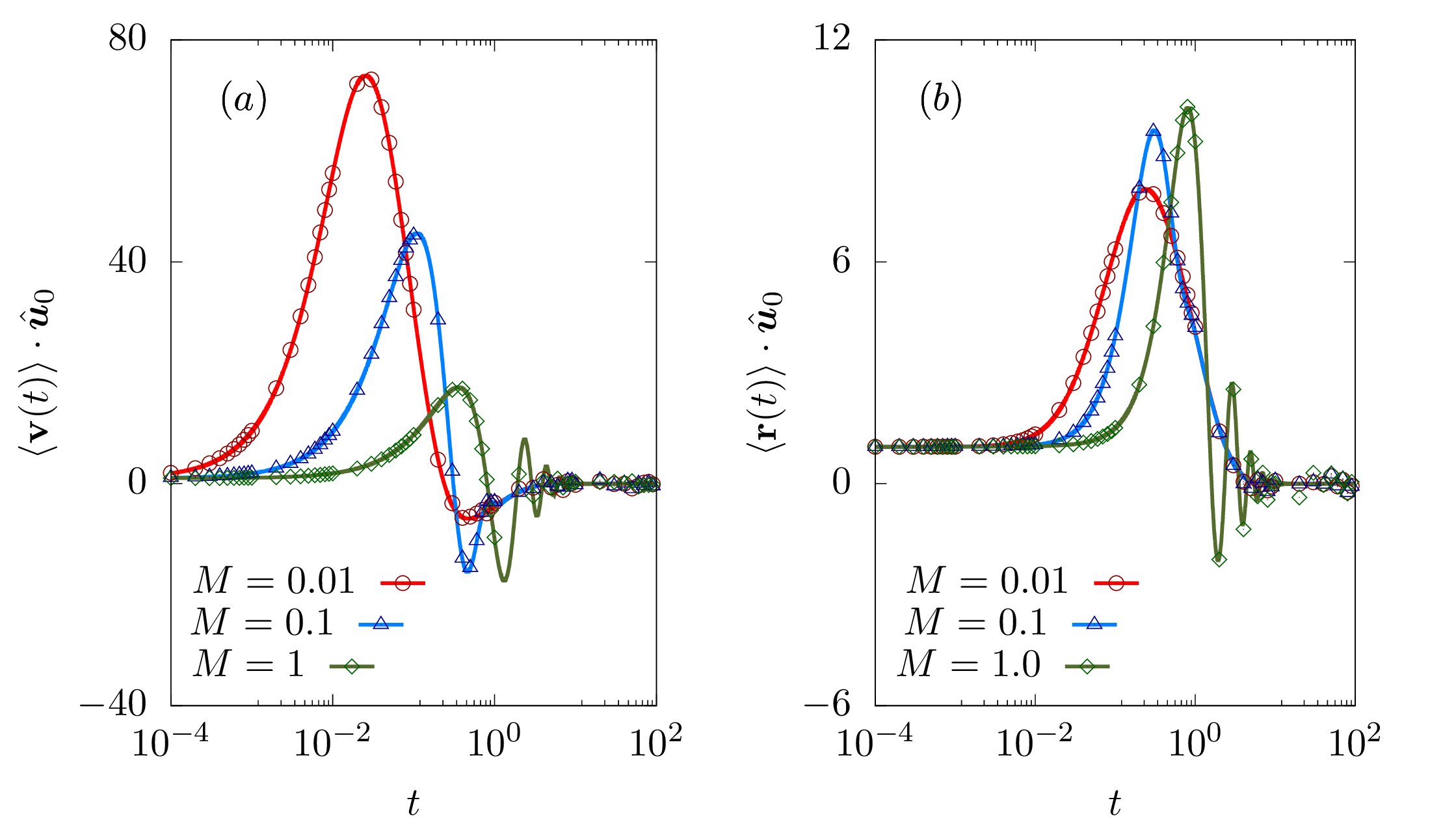
Figure 1: Time evolution of first moments $\langle{\mathbf{v}}(t)\rangle$ ($a$) and $\langle{\mathbf{r}}(t)\rangle$ ($b$) projected along initial orientation $\hat{\bm{u}}_{0}$ in $d=2$ dimensions. The solid lines are obtained from equations (3.1) and (3.1), respectively. The points denote simulation results. The plots correspond to ${\rm Pe}=100$, $\beta=10$, and initial conditions ${\mathbf{r}}_{0}=(1,0)$, ${\mathbf{v}}_{0}=(1,0)$, and $\hat{\bm{u}}_{0}=(1,0)$.

3 First moments

We begin by utilizing equation (6) to obtain the time evolution of several first-order moments, such as the mean velocity, position, and heading direction. In the presence of a harmonic trap, the dynamics of velocity and position both evolve to reach a steady state.

3.1 Mean velocity, position and heading direction

Utilizing $\psi={\mathbf{v}}$ in equation (6), we get the mean velocity in the Laplace space $\langle{\mathbf{v}}\rangle_{s}=[{\mathbf{v}}_{0}+({\rm Pe}/M)\langle\hat{\bm{u}}\rangle_{s}-(\beta/M)\langle{\mathbf{r}}\rangle_{s}]/(s+1/M)$ in the terms of $\langle{\mathbf{r}}\rangle_{s}$ and $\langle\hat{\bm{u}}\rangle_{s}$. Again, using $\psi={\mathbf{r}}$ and $\psi=\hat{\bm{u}}$, equation (6) gives $\langle{\mathbf{r}}\rangle_{s}=[\langle{\mathbf{v}}\rangle_{s}+{\mathbf{r}}_{0}]/s$ and $\langle\hat{\bm{u}}\rangle_{s}=\hat{\bm{u}}_{0}/(s+d-1)$, respectively. The solution of these coupled equations leads to

$$\langle{\mathbf{v}}\rangle_{s}=\frac{(sM{\mathbf{v}}_{0}-\beta\,{\mathbf{r}}_{0})}{Ms^{2}+s+\beta}+\frac{s{\rm Pe}\,\hat{\bm{u}}_{0}}{(s+d-1)(Ms^{2}+s+\beta)},$$ (7)

$$\langle{\mathbf{r}}\rangle_{s}=\frac{M{\mathbf{v}}_{0}+(1+sM){\mathbf{r}}_{0}}{Ms^{2}+s+\beta}+\frac{{\rm Pe}\,\hat{\bm{u}}_{0}}{(s+d-1)(Ms^{2}+s+\beta)}.$$ (8)

The inverse Laplace transform of equation (7) and $\langle\hat{\bm{u}}\rangle_{s}$ gives the full-time evolution which can be expressed as

$$\langle{\mathbf{v}}\rangle(t)=-\frac{(d-1){\rm Pe}\,\hat{\bm{u}}_{0}}{{\cal C}_{1}}e^{-(d-1)t}+\frac{1}{2}\left({\mathbf{v}}_{0}+\frac{{(d-1)\rm Pe}\,\hat{\bm{u}}_{0}}{{\cal C}_{1}}\right)\left[e^{-\alpha_{+}t/2}+e^{-\alpha_{-}t/2}\right]$$

$$+\frac{1}{2i\omega{\cal C}_{1}}\left\{(d-1)[{\rm Pe}\,\hat{\bm{u}}_{0}+((d-1)M-1){\mathbf{v}}_{0}]+\beta[2(d-1)((d-1)M-1){\mathbf{r}}_{0}\right.$$

$$\left.-2{\rm Pe}\,\hat{\bm{u}}_{0}+{\mathbf{v}}_{0}]+2\beta^{2}{\mathbf{r}}_{0}\right\}\left[e^{-\alpha_{+}t/2}-e^{-\alpha_{-}t/2}\right],$$ (9)

where

$$\omega=\sqrt{4\beta M-1},$$

$$\alpha_{\pm}=\frac{1}{M}[1\pm i\omega],$$

$${\cal C}_{1}=(d-1)^{2}M-(d-1)+\beta,$$ (10)

and $\langle\hat{\bm{u}}\rangle(t)=\hat{\bm{u}}_{0}e^{-(d-1)t}$. The mean velocity vanishes in the steady-state $\langle{\mathbf{v}}\rangle_{\rm st}=0$. Before vanishing, it shows an oscillatory decay with frequency $\omega/M$ if $\beta M>1/4$, the imaginary part of $\alpha_{\pm}$. The case of $4\beta M=1$ corresponds to critical damping in oscillations. In the limit of vanishing trap strength, equation (3.1) reduces to the known expression for free iABPs [55].

Likewise, the inverse Laplace transform of equation (8) gives the full-time evolution of mean position as

$$\langle{\mathbf{r}}\rangle(t)=\frac{{\rm Pe}\,\hat{\bm{u}}_{0}}{{\cal C}_{1}}e^{-(d-1)t}+\frac{1}{2i\omega}\left({\mathbf{r}}_{0}+2M{\mathbf{v}}_{0}+\frac{[2M(d-1)-1]{\rm Pe}\,\hat{\bm{u}}_{0}}{{\cal C}_{1}}\right)\left[e^{-\alpha_{-}t/2}\right.$$

$$\left.-e^{-\alpha_{+}t/2}\right]+\frac{1}{2}\left({\mathbf{r}}_{0}-\frac{{\rm Pe}\,\hat{\bm{u}}_{0}}{{\cal C}_{1}}\right)\left[e^{-\alpha_{-}t/2}+e^{-\alpha_{+}t/2}\right].$$ (11)

In the steady state, the mean position also vanishes $\langle{\mathbf{r}}\rangle_{\rm st}=0$ and shows an oscillatory evolution towards the steady state with frequency $\omega/M$ if $\beta M>1/4$, as for mean velocity. In the limit of vanishing inertia, equation (3.1) restores the previously known result of overdamped trapped ABPs [52], and in the vanishing trap strength, it restores the result of free iABPs [55].

In figure 1, we show projections of mean velocity and position along the initial orientation evolving towards the steady state. Two distinct kinds of evolutions are observed. For $4\beta M>1$, $\alpha_{\pm}$ has an imaginary part, which sets oscillation with $\omega/M$ frequency and a real part which governs the decay in time with a time constant $2M$ for both $\langle{\mathbf{r}}\rangle(t)$ and $\langle{\mathbf{v}}\rangle(t)$, as shown for $M=0.1,1$ in figure 1 in two dimensions (2d). However, at $4\beta M<1$, $\alpha_{\pm}$ is real, and the solution of $\langle{\mathbf{r}}\rangle(t)$ and $\langle{\mathbf{v}}\rangle(t)$ decays to zero asymptotically in a non-monotonic manner that lacks oscillation. This is shown for $M=0.01$ in figure 1. The moments $\langle{\mathbf{r}}(t)\rangle\cdot\hat{\bm{u}}_{0}$ and $\langle{\mathbf{v}}(t)\rangle\cdot\hat{\bm{u}}_{0}$ starts from $\hat{\bm{u}}_{0}\cdot{\mathbf{r}}_{0}$ and $\hat{\bm{u}}_{0}\cdot{\mathbf{v}}_{0}$, respectively at the short time. From equations (7) and (8), it is easy to see that, in the presence of the trap, the steady-state values vanish, $\langle{\mathbf{v}}\rangle_{\rm st}=\lim_{s\to 0+}s\langle{\mathbf{v}}\rangle_{s}=0$ and $\langle{\mathbf{r}}\rangle_{\rm st}=\lim_{s\to 0+}s\langle{\mathbf{r}}\rangle_{s}=0$.

4 Second Moments: Mean-Squared Displacement and Kinetic Temperature

In this section, we explore the time evolution of second moments, including the projection of position and velocity towards instantaneous heading direction, mean squared displacement (MSD), and mean squared velocity (MSV). Note that the projections involve cross-correlation of position and velocity with orientation.

4.1 Position and velocity component in heading direction

The simplest second moments are inner products of velocity and displacement variables with instantaneous orientation, in other words, their components along the heading direction. We use $\psi=v_{\parallel}=\hat{\bm{u}}\cdot{\mathbf{v}}$ in equation (6) to get $[s+1/M+(d-1)]\langle v_{\parallel}\rangle_{s}=\hat{\bm{u}}_{0}\cdot{\mathbf{v}}_{0}+{\rm Pe}/(sM)-(\beta/M)\langle\hat{\bm{u}}\cdot{\mathbf{r}}\rangle_{s},$ in terms of $\langle\hat{\bm{u}}\cdot{\mathbf{r}}\rangle_{s}$. Again using $\psi=r_{\parallel}=\hat{\bm{u}}\cdot{\mathbf{r}}$ in equation (6), we get $[s+(d-1)]\langle r_{\parallel}\rangle_{s}=\hat{\bm{u}}_{0}\cdot{\mathbf{r}}_{0}+\langle v_{\parallel}\rangle_{s}$. The solution of these coupled equations gives $\langle v_{\parallel}\rangle_{s}$ and $\langle r_{\parallel}\rangle_{s}$ as

$$\langle v_{\parallel}\rangle_{s}=\frac{[s+(d-1)]({\rm Pe}+sM\hat{\bm{u}}_{0}\cdot{\mathbf{v}}_{0})-s\beta\hat{\bm{u}}_{0}\cdot{\mathbf{r}}_{0}}{s[\beta+(s+d-1)\{M(s+d-1)+1\}]},$$ (12)

$$\langle r_{\parallel}\rangle_{s}=\frac{{\rm Pe}+s\left[\{M(s+d-1)+1\}\hat{\bm{u}}_{0}\cdot{\mathbf{r}}_{0}+M\hat{\bm{u}}_{0}\cdot{\mathbf{v}}_{0}\right]}{s[\beta+(s+d-1)\{M(s+d-1)+1\}]}.$$ (13)

The inverse Laplace transform of the above equations give

$$\langle v_{\parallel}\rangle(t)=\frac{(d-1){\rm Pe}}{{\cal C}_{2}}+\frac{1}{2i\omega}\left[\frac{(d-1+2\beta){\rm Pe}}{{\cal C}_{2}}-2\beta\hat{\bm{u}}_{0}\cdot{\mathbf{r}}_{0}-\hat{\bm{u}}_{0}\cdot{\mathbf{v}}_{0}\right]\left(e^{-\{\alpha_{-}+2(d-1)\}t/2}\right.$$

$$\left.-e^{-\{\alpha_{+}+2(d-1)\}t/2}\right)-\frac{1}{2}\left[\frac{(d-1){\rm Pe}}{{\cal C}_{2}}-\hat{\bm{u}}_{0}\cdot{\mathbf{v}}_{0}\right]\left(e^{-\{\alpha_{-}+2(d-1)\}t/2}+e^{-\{\alpha_{+}+2(d-1)\}t/2}\right),$$ (14)

and

$$\langle r_{\parallel}\rangle(t)=\frac{{\rm Pe}}{{\cal C}_{2}}+\frac{1}{2i\omega}\left[\frac{(1+2M(d-1)){\rm Pe}}{{\cal C}_{2}}-\hat{\bm{u}}_{0}\cdot{\mathbf{r}}_{0}-2M\hat{\bm{u}}_{0}\cdot{\mathbf{v}}_{0}\right]\left(e^{-\{\alpha_{+}+2(d-1)\}t/2}\right.$$

$$\left.-e^{-\{\alpha_{-}+2(d-1)\}t/2}\right)-\frac{1}{2}\left[\frac{{\rm Pe}}{{\cal C}_{2}}-\hat{\bm{u}}_{0}\cdot{\mathbf{r}}_{0}\right]\left(e^{-\{\alpha_{-}+2(d-1)\}t/2}+e^{-\{\alpha_{+}+2(d-1)\}t/2}\right),$$ (15)

with

$${\cal C}_{2}=(d-1)^{2}M+(d-1)+\beta.$$ (16)

In the asymptotic limit, the two projections $\langle v_{\parallel}\rangle$ and $\langle r_{\parallel}\rangle$ approach the steady state values ${\rm Pe}/[(d-1)M+1+\beta/(d-1)]$ and ${\rm Pe}/[(d-1)^{2}M+d-1+\beta]$ respectively. In the vanishing trap strength limit, $\langle v_{\parallel}\rangle_{\rm st}$ takes the previously known form of free iABPs [55]. In the other limit of $\beta\to\infty$, both projections $\langle r_{\parallel}\rangle_{\rm st}$ and $\langle v_{\parallel}\rangle_{\rm st}$ vanishes.

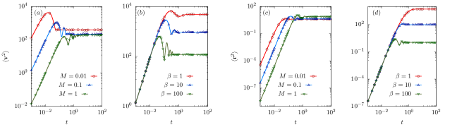
Figure 2: Time evolution of second moments $\langle{\mathbf{v}}^{2}\rangle(t)$ and $\langle{\mathbf{r}}^{2}\rangle(t)$ in $d$ = 2. We show the evolution of $\langle{\mathbf{v}}^{2}\rangle$ and $\langle{\mathbf{r}}^{2}\rangle$ for different $M$ values at $\beta=50$ ($a$), ($c$) and for different $\beta$ values at $M=0.1$ ($b$), ($d$). The plots use ${\rm Pe}=100$, ${\mathbf{r}}_{0}=(0,0)$, ${\mathbf{v}}_{0}=(0,0)$ and $\hat{\bm{u}}_{0}=(1,0)$. The lines correspond to equation (4.2) in ($a$), ($b$) and equation (4.3) in ($c$), ($d$). The points denote simulation results.

4.2 Mean Squared Velocity

We set $\psi={\mathbf{v}}^{2}$ in equation (6) to find the second moment of velocity. We use the following relations: ${\mathbf{v}}\cdot\nabla\psi=0$, $\langle{\mathbf{v}}\cdot\nabla_{v}\psi\rangle_{s}=2\,\langle{\mathbf{v}}^{2}\rangle_{s}$, $\langle\hat{\bm{u}}\cdot\nabla_{v}\psi\rangle_{s}=2\,\langle v_{\parallel}\rangle_{s}$, $\langle{\mathbf{r}}\cdot\nabla_{v}\psi\rangle_{s}=2\,\langle{\mathbf{v}}\cdot{\mathbf{r}}\rangle_{s}$, $\langle\nabla_{v}^{2}\psi\rangle_{s}=2d\langle 1\rangle_{s}=2d/s$   and $\nabla_{u}^{2}\psi=0$, to get

$$(s+2/M)\langle{\mathbf{v}}^{2}\rangle_{s}={\mathbf{v}}_{0}^{2}+(2\,{\rm Pe}/M)\langle v_{\parallel}\rangle_{s}-(2\beta/M)\langle{\mathbf{v}}\cdot{\mathbf{r}}\rangle_{s}+2d/(sM^{2}),$$ (17)

where $\langle v_{\parallel}\rangle_{s}$ is already known from equation (12). We further calculate $\langle{\mathbf{v}}\cdot{\mathbf{r}}\rangle_{s}$, by inserting $\psi={\mathbf{v}}\cdot{\mathbf{r}}$ in equation (6) to get

$$(s+1/M)\langle{\mathbf{v}}\cdot{\mathbf{r}}\rangle_{s}={\mathbf{v}}_{0}\cdot{\mathbf{r}}_{0}+\langle{\mathbf{v}}^{2}\rangle_{s}+({\rm Pe}/M)\langle r_{\parallel}\rangle_{s}-(\beta/M)\langle{\mathbf{r}}^{2}\rangle_{s},$$ (18)

where $\langle r_{\parallel}\rangle_{s}$ is given by equation (13). Completing the calculation further requires the second moment of position $\langle{\mathbf{r}}^{2}\rangle_{s}$. Using $\psi={\mathbf{r}}^{2}$ in equation  (6) we get

$$s\langle{\mathbf{r}}^{2}\rangle_{s}={\mathbf{r}}_{0}^{2}+2\langle{\mathbf{v}}\cdot{\mathbf{r}}\rangle_{s}.$$ (19)

Equations (17) to (19) give the required moments in the Laplace space. For the choice of initial condition ${\mathbf{v}}_{0}=\bf{0}$ and ${\mathbf{r}}_{0}=\bf{0}$, the expression simplifies significantly and gives the MSV

$$\langle{\mathbf{v}}^{2}\rangle_{s}=\frac{2}{{\cal B}_{0}}\left(s(s+d-1)(sM+1)[d(d+1)M+M{\rm Pe}^{2}+dM(s-1)]+2d\beta^{2}\right.$$

$$\left.+\beta\left[2(d-1)\{d((d-1)M+1)+M{\rm Pe}^{2}\}+sd\{3+4M(d-1)\}+sM{\rm Pe}^{2}+3dMs^{2}\right]\right),$$

and cross-correlation

$$\langle{\mathbf{v}}\cdot{\mathbf{r}}\rangle_{s}=\frac{sM}{{\cal B}_{0}}\left({\rm Pe}^{2}[(3s-2)M+2]+2d[s+\beta-1+M((s-1)^{2}+{\rm Pe}^{2})]\right.$$

$$\left.+d^{2}[4M(s-1)+2]+2d^{3}M\right),$$ (21)

where ${\cal B}_{0}=sM(sM+1)\{s(sM+2)+4\beta\}\{(s+d-1)[(s+d-1)M+1]+\beta\}$. It is easy to check that the steady state cross-correlation $\langle{\mathbf{v}}\cdot{\mathbf{r}}\rangle_{st}=\lim_{s\to 0+}s\langle{\mathbf{v}}\cdot{\mathbf{r}}\rangle_{s}=0$.

The inverse Laplace transform of equation (4.2) gives the full-time evolution of MSV,

$$\langle{\mathbf{v}}^{2}\rangle(t)=\frac{d}{M}+\frac{(d-1){\rm Pe}^{2}}{{\cal C}_{2}}+\frac{2\beta}{\omega^{2}}\left(-2d+\frac{[1-2(d-1)M]{\rm Pe}^{2}}{{\cal C}_{1}}\right)e^{-t/M}$$

$$-\frac{(d-1){\rm Pe}^{2}}{i\omega{\cal C}_{1}{\cal C}_{2}}\left([2\beta+(d-1)M\alpha_{-}]e^{-\{\alpha_{-}+2(d-1)\}t/2}-[2\beta+(d-1)M\alpha_{+}]e^{-\{\alpha_{+}+2(d-1)\}t/2}\right)$$

$$+\frac{1}{2\omega^{2}{\cal C}_{1}}\left(d\alpha_{-}\left[{\cal C}_{1}+M{\rm Pe}^{2}\right]-{\rm Pe}^{2}\{M\alpha_{-}+2\beta\}\right)e^{-\alpha_{-}t}$$

$$+\frac{1}{2\omega^{2}{\cal C}_{1}}\left(d\alpha_{+}\left[{\cal C}_{1}+M{\rm Pe}^{2}\right]-{\rm Pe}^{2}\{M\alpha_{+}+2\beta\}\right)e^{-\alpha_{+}t}.$$ (22)

As shown in the figure 2($a$,$b$), the plot of the above equation agrees with the numerical simulation results of MSV in 2d. The evolution in harmonic trap shows oscillations before saturating to steady state values determined by ${\rm Pe}$, $M$, and $\beta$. In the limit of vanishing trap strength, MSV takes the form of free iABPs [55]. The short-time evolution can be further analyzed using an expansion of $\langle{\mathbf{v}}^{2}\rangle(t)$ around $t=0$

$$\langle{\mathbf{v}}^{2}\rangle(t)=\frac{2d}{M^{2}}t+\frac{(M{\rm Pe}^{2}-2d)}{M^{3}}t^{2}-\frac{[2d(\beta M-2)+M\,{\rm Pe}^{2}\{3+(d-1)M\}]}{3M^{4}}t^{3}+{\cal O}(t^{4})$$

It takes time, determined by inertia and trap strength, before the influence of activity, and subsequently, the harmonic trap shows up in the evolution of ${\mathbf{v}}^{2}(t)$. MSV shows a diffusive scaling similar to free iABPs in the shortest time [55]. The expansion shows a diffusive $\langle{\mathbf{v}}^{2}\rangle\sim t$ to ballistic $\langle{\mathbf{v}}^{2}\rangle\sim t^{2}$ crossover at $t_{I}=2dM/(M{\rm Pe}^{2}-2d)$, which depends on $M$ but is independent of $\beta$. At high ${\rm Pe}$, it shows non-monotonicity at a later time and decreases as $\langle{\mathbf{v}}^{2}\rangle\sim\,-t^{3}$ beyond $t_{II}=(3M({\rm Pe}^{2}M-2d))/[2d(\beta M-2)+M\,{\rm Pe}^{2}\{3+(d-1)M\}]$ (figure 2($a$) ). This crossover time depends on the trap strength $\beta$, which also causes subsequent oscillations before reaching a steady state. The asymptotic steady-state value of MSV is given by

$$\langle{\mathbf{v}}^{2}\rangle_{\rm st}=\frac{d}{M}+\frac{(d-1){\rm Pe}^{2}}{(d-1)^{2}M+(d-1)+\beta},$$ (24)

which decreases with both $M$ and $\beta$. In the limit of $\beta\rightarrow 0$, $\langle{\mathbf{v}}^{2}\rangle_{\rm st}$ reduces to the previously known form of free iABPs [55].

In figure 3(a) and (b), parameter dependence of steady-state MSV, $\langle{\mathbf{v}}^{2}\rangle_{\rm st}$, are shown. They start from maximum value $d/M+{\rm Pe}^{2}/[(d-1)M+1]$ at small $M$ and $\beta$ to decrease with increasing inertia and trap stiffness. Since $\langle{\mathbf{v}}\rangle_{\rm st}=0$, the steady-state velocity fluctuation is also given by the MSV, $\langle\delta{\mathbf{v}}^{2}\rangle_{\rm st}=\langle{\mathbf{v}}^{2}\rangle_{\rm st}$.

4.3 Mean Squared Displacement

Using equations (17) to (19) we obtain the MSD in Laplace space. With the initial condition ${\mathbf{v}}_{0}=\bf{0}$ and ${\mathbf{r}}_{0}=\bf{0}$, the expression for MSD simplifies to

$$\langle{\mathbf{r}}^{2}\rangle_{s}=\frac{M}{{\cal B}_{0}}\left(4d\{s-1+\beta+M[(s-1)^{2}+{\rm Pe}^{2}]\}+d^{2}[8M(s-1)+4]+4d^{3}M\right.$$

$$\left.+2{\rm Pe}^{2}[M(3s-2)+2]\right)$$ (25)

where ${\cal B}_{0}$ has the same $s$-dependent form as used before to describe $\langle{\mathbf{v}}^{2}\rangle_{s}$. The inverse Laplace transform of this relation reads

$$\langle{\mathbf{r}}^{2}\rangle(t)=\frac{d}{\beta}+\frac{{\rm Pe}^{2}(1+(d-1)M)}{\beta{\cal C}_{2}}+\frac{2M}{\omega^{2}}\left(-2d+\frac{(1-2M(d-1)){\rm Pe}^{2}}{{\cal C}_{1}}\right)e^{-t/M}$$

$$-\frac{\left[\alpha_{+}+2(d-1)\,\right]M{\rm Pe}^{2}}{i\omega{\cal C}_{1}{\cal C}_{2}}e^{-\{\alpha_{-}+2(d-1)\}t/2}+\frac{\left[\alpha_{-}+2(d-1)\,\right]M{\rm Pe}^{2}}{i\omega{\cal C}_{1}{\cal C}_{2}}e^{-\{\alpha_{+}+2(d-1)\}t/2}$$

$$+\frac{1}{2i\beta\omega^{3}{\cal C}_{1}}\left(i\omega dM\alpha_{-}\left[{\cal C}_{1}+M{\rm Pe}^{2}\right]+{\rm Pe}^{2}\left[M\alpha_{-}(1+M-2\beta M)-2\beta M(1+2M)\right]\right)e^{-\alpha_{+}t}$$

$$+\frac{1}{2i\beta\omega^{3}{\cal C}_{1}}\left(i\omega dM\alpha_{+}\left[{\cal C}_{1}+M{\rm Pe}^{2}\right]-{\rm Pe}^{2}\left[M\alpha_{+}(1+M-2\beta M)-2\beta M(1+2M)\right]\right)e^{-\alpha_{-}t}.$$

The above equation captures the evolution of MSD as seen in numerical simulation in $2$d, shown in figure 2($c$,$d$). The expression of MSD reduces to that of the overdamped case in the limit of vanishing inertia [52] while it restores the result of free iABPs in the limit of vanishing trap strength [55]. To analyze the crossovers at a short time, we expand $\langle{\mathbf{r}}^{2}\rangle$ around $t=0$

$$\langle{\mathbf{r}}^{2}\rangle(t)=\frac{2d}{3M^{2}}t^{3}+\frac{(M{\rm Pe}^{2}-2d)}{4M^{3}}t^{4}-\frac{\{d(4\beta M-7)+M\,{\rm Pe}^{2}[5+2(d-1)M]\}}{30M^{4}}t^{5}+{\cal O}(t^{6}).$$

MSD shows $\sim t^{3}$ scaling at the shortest time scale similar to free iABPs [55]. The influence of activity shows up in the form of a $\langle{\mathbf{r}}^{2}\rangle\sim t^{3}$ to $\langle{\mathbf{r}}^{2}\rangle\sim t^{4}$ crossover at time $t_{I}=8dM/[3(M{\rm Pe}^{2}-2d)]$. A subsequent crossover towards saturation of MSD appears approximately at $t_{II}\approx 15M(2d-{\rm Pe}^{2}M)/(2\{d(4\beta M-7)+M\,{\rm Pe}^{2}[5+2(d-1)M]\})$, due to the trap and as a result depends on the trap strength $\beta$. In the asymptotic limit, MSD reaches the steady state value

$$\langle{\mathbf{r}}^{2}\rangle_{\rm st}=\frac{d}{\beta}+\frac{{\rm Pe}^{2}(1+(d-1)M)}{\beta[(d-1)^{2}M+(d-1)+\beta]}\,,$$ (28)

which depends on both $M$ and $\beta$. In the limit of vanishing $M$, the above expression for $\langle{\mathbf{r}}^{2}\rangle_{\rm st}$ reduces to the previously known form of MSD in overdamped trapped ABPs [52]. The MSD increases with $M$ to saturate to $\lim_{M\to\infty}[\langle{\mathbf{r}}^{2}\rangle_{\rm st}]=(d/\beta+{\rm Pe}^{2}/\beta(d-1))$. In figure 3(a) and (b), such dependence of steady-state MSD, $\langle{\mathbf{r}}^{2}\rangle_{\rm st}$, are shown. With $M$, it increases to saturate to $(d/\beta+{\rm Pe}^{2}/\beta(d-1))$. However, with $\beta$, it monotonically decreases from the $1/\beta$ divergence at $\beta\to 0$ to vanishing as $1/\beta^{2}$ in the large $\beta$ limit.

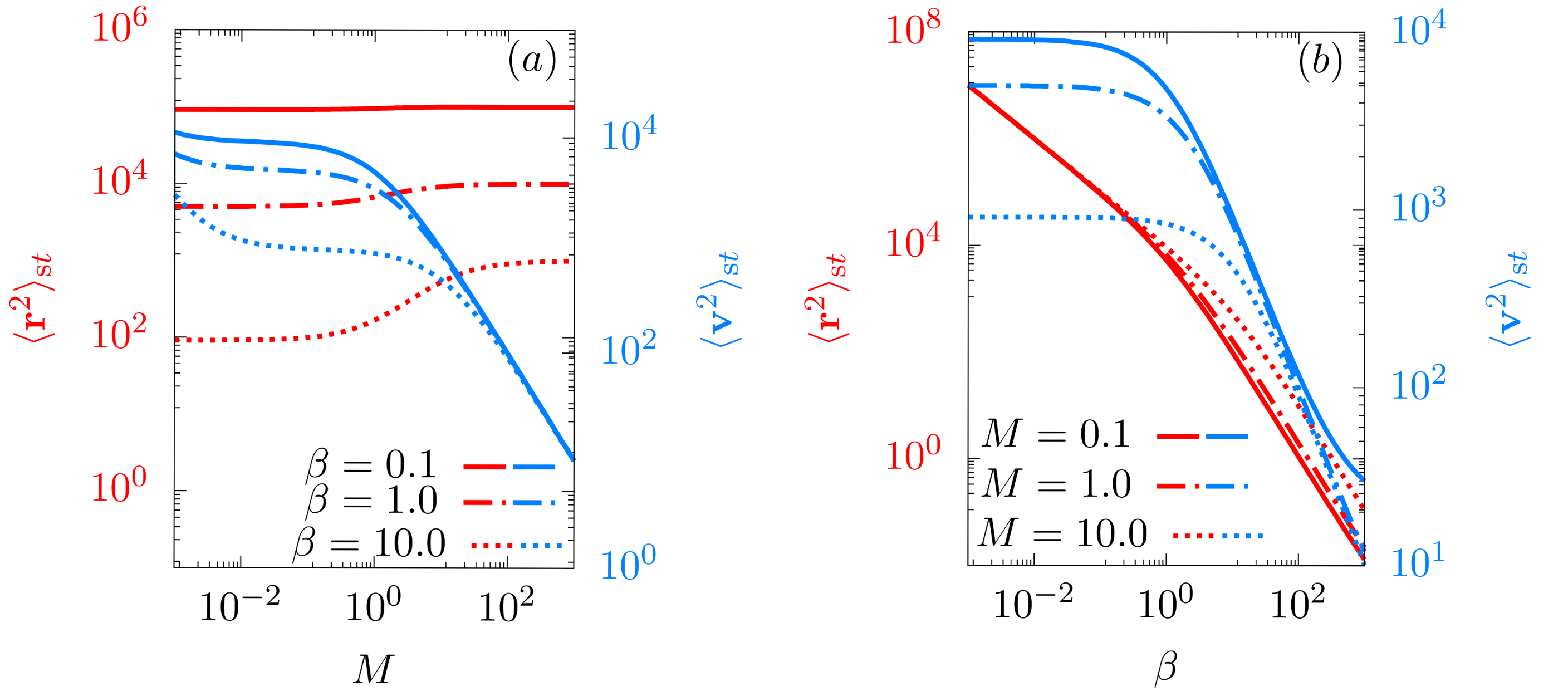
Figure 3: The steady-state of second moments $\langle{\mathbf{v}}^{2}\rangle_{\rm st}$ (blue), $\langle{\mathbf{r}}^{2}\rangle_{\rm st}$ (red) as a function of $M$ ($a$) and $\beta$ ($b$) in $2$d. The lines are plots of equations (24) and (28) at ${\rm Pe}=100$.

4.4 Estimates of kinetic temperature, diffusivity, and violation of equilibrium fluctuation-dissipation relation

The steady-state expressions for MSV and MSD, derived above, can be used to obtain asymptotic estimates of kinetic temperature and diffusivity of iABP in traps. The fluctuation in velocity leads to the following estimate for kinetic temperature,

$$k_{\rm B}T_{\rm kin}=\frac{M\langle{\mathbf{v}}^{2}\rangle_{\rm st}}{d}=1+\frac{M(d-1){\rm Pe}^{2}}{d[(d-1)^{2}M+(d-1)+\beta]}.$$ (29)

In contrast to trapped Brownian motion in equilibrium, this estimate depends explicitly on inertia $M$ and trap strength $\beta$.

In the vanishing $\beta$ limit, the expression agrees with the earlier estimate for free iABPs [55]. In the overdamped limit $M\rightarrow 0$, the dimensionless $k_{B}T_{\rm kin}=1$, set by translational diffusivity. At small $M$, $k_{B}T_{\rm kin}$ increases linearly with $M$ to saturate to $1+{\rm Pe}^{2}/[d(d-1)]$, independent of $\beta$. However, at a given $M$, the dimensionless $k_{B}T_{\rm kin}$ decreases with $\beta$ to saturate to unity.

The fluctuation in position at equilibrium gives $\langle{\mathbf{r}}^{2}\rangle_{eq}=d\,D/\beta D_{r}$ with equilibrium fluctuation-dissipation relation (FDR) $D=\mu k_{B}T$. In the absence of such FDR, the out-of-equilibrium steady-state fluctuation can not be associated with such a unique definition of temperature. However, extending this notion, one can obtain the following estimate for the effective diffusivity

$$D_{\rm eff}:=\frac{\beta\langle{\mathbf{r}}^{2}\rangle_{\rm st}}{d}=1+\frac{{\rm Pe}^{2}}{d[(d-1)+\frac{\beta}{1+(d-1)M}]},$$ (30)

in the dimensionless form, replacing $D_{\rm eff}/D$ by $D_{\rm eff}$ and using unity for $l^{-2}=D_{r}/D$ as $l$ sets the unit of length in the first expression presented above. It is important to note that $D_{\rm eff}$ depends on both $M$ and $\beta$, where the $M$ dependence enters through the potential strength $\beta$. Remarkably, numerical simulations of interacting iABPs display inertia-dependent diffusivity [56], a behavior qualitatively similar to the above relation.

In the free particle limit of $\beta\to 0$, the active part of diffusivity reduces to ${\rm Pe}^{2}/d(d-1)$, a result established before for free iABP [55] and indistinguishable from overdamped ABPs. Moreover, in the vanishing $M$ limit, $D_{\rm eff}=1+{\rm Pe}^{2}/[d(\beta+d-1)]$. With increasing $M$, $D_{\rm eff}$ increases to saturate to the free iABP diffusivity $1+{\rm Pe}^{2}/[d(d-1)]$.

The departure from equilibrium FDR in the dimensionless form can be expressed as

$${\cal I}:=D_{\rm eff}-k_{\rm B}T_{\rm kin}=\frac{{\rm Pe}^{2}}{d[(d-1)^{2}M+(d-1)+\beta]},$$ (31)

where in the first relation, we replaced $\mu k_{\rm B}T_{\rm kin}/D$ by the dimensionless form of kinetic temperature $k_{\rm B}T_{\rm kin}$. The violation of equilibrium FDR is the maximum for vanishing $M$ and $\beta$. It decreases with increasing $M$ and $\beta$ to vanish as $M^{-1}$ and $\beta^{-1}$. In the vanishing $\beta$ limit, the above expression reduces to the known form for free iABPs [55].

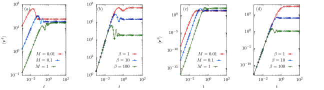
Figure 4: Time evolution of fourth moments $\langle{\mathbf{v}}^{4}\rangle(t)$ and $\langle{\mathbf{r}}^{4}\rangle(t)$ in $d$ = 2. The evolution of $\langle{\mathbf{v}}^{4}\rangle$ and $\langle{\mathbf{r}}^{4}\rangle$ for different $M$ values at $\beta=50$ ($a$), ($c$) and for different $\beta$ values at $M=0.1$ ($b$), ($d$). The plots use ${\rm Pe}=100$, ${\mathbf{r}}_{0}=(0,0)$, ${\mathbf{v}}_{0}=(0,0)$ and $\hat{\bm{u}}_{0}=(1,0)$. The lines correspond to analytic estimates, and points denote simulation results.

5 Fourth Moments

In this section, we discuss the time evolution of fourth moments of dynamics, such as velocity and displacement, and the dependence of their steady-state values on control parameters. A stochastic process can be distinguished from the Gaussian process using kurtosis, which involves the fourth moment of the corresponding random variable. We present such analyses for velocity and displacement with the help of excess kurtosis.

5.1 Fourth Moment of Velocity and Displacement

The calculation for fourth moments in Laplace space, $\langle{\mathbf{r}}^{4}\rangle_{s}$ and $\langle{\mathbf{v}}^{4}\rangle_{s}$, follows the same steps shown before for other moments and utilizes equation (6). Despite being lengthy, these calculations are straightforward. We show the essential steps for the calculations in Laplace space in A. The inverse Laplace transform gives the full-time evolution. Instead of showing these long expressions for time-dependence, we plot them for $\langle{\mathbf{r}}^{4}\rangle(t)$ and $\langle{\mathbf{v}}^{4}\rangle(t)$ and compare them with numerical simulation results in $2$d in figure 4. The results are shown for a range of $M$ and $\beta$ values at ${\rm Pe}=100$. The simulation results show excellent agreement with analytic estimates. Apart from plotting the expressions, we present series expansions of them around $t=0$ to analyze their short-time behavior and also present the explicit steady-state expressions. The series expansion of $\langle{\mathbf{v}}^{4}\rangle(t)$ around $t=0$ in 2d (see B for $d=3$ dimensions) using initial values ${\mathbf{r}}_{0}=\bf{0}$ and ${\mathbf{v}}_{0}=\bf{0}$ is given by

$$\langle{\mathbf{v}}^{4}\rangle(t) =\frac{32}{M^{4}}t^{2}+\frac{16(M{\rm Pe}^{2}-4)}{M^{5}}t^{3}$$ (32)

$$+\frac{[224+M\{-64\beta-16(6+M){\rm Pe}^{2}+3M{\rm Pe}^{4}\}]}{3M^{6}}t^{4}+{\cal O}{(t^{5})}.$$

The expansion shows an initial $t^{2}$ dependence for a short time, which crosses over to $t^{3}$ behavior at $t_{I}=2M/(M{\rm Pe}^{2}-4)$ which depends on $M$ but independent of $\beta$, a behavior similar to free iABPs [55]. The impact of trapping is felt only at a later time $t_{II}=48M(M{\rm Pe}^{2}-4)/[224+M\{-64\beta-16(6+M){\rm Pe}^{2}+3M{\rm Pe}^{4}\}]$ leading to a departure from the $t^{3}$ behavior.

The steady-state value of the fourth velocity moment in 2d (see B for $d=3$ dimension) is given by

$$\langle{\mathbf{v}}^{4}\rangle_{\rm st}=\frac{8}{M^{2}}+\frac{8}{M(1+\beta+M)}{\rm Pe}^{2}+\frac{{\cal A}_{1}}{{\cal B}_{1}}{\rm Pe}^{4}$$ (33)

where ${\cal A}_{1}=\{\beta\left[162+M\{1209+M(2575+2M(993+4M(71+16M)))\}\right]+\beta^{2}M[297$ $+2M(567+882M+592M^{2})]+6(1+M)(2+M)(1+4M)(3+4M)+36\beta^{3}M^{2}(3+8M)\}$ and ${\cal B}_{1}=[(1+\beta+M)(3+9\beta+M)(1+4M)(2+\beta+4M)(3+4\beta M)(2+M(3+\beta+M))]$. Figure 5 shows $M$ and $\beta$ dependence of $\langle{\mathbf{v}}^{4}\rangle_{\rm st}$ at ${\rm Pe}=100$, displaying overall decreases of the moment with both the parameters.

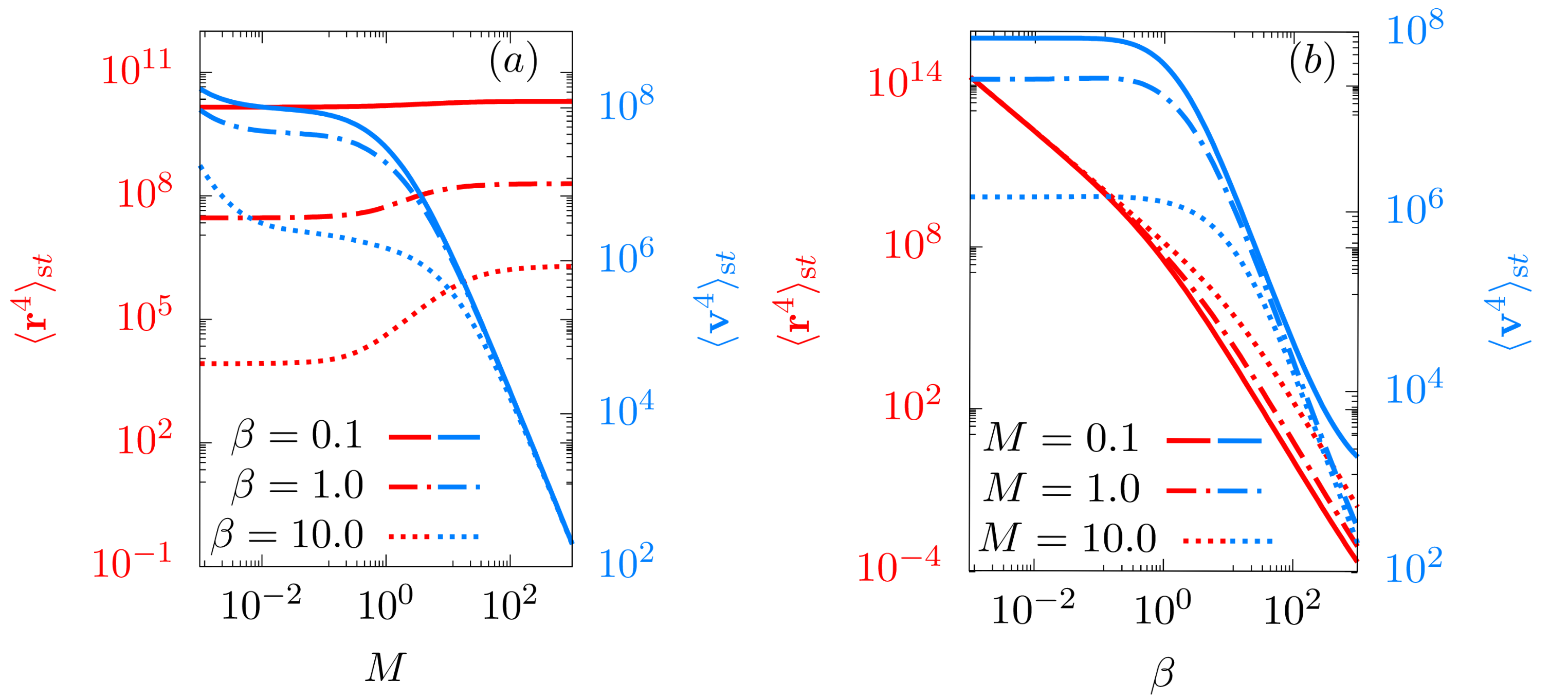
Figure 5: The steady-state of fourth moments $\langle{\mathbf{v}}^{4}\rangle_{\rm st}$, $\langle{\mathbf{r}}^{4}\rangle_{\rm st}$ as a function of $M$ ($a$) and $\beta$ ($b$) in $2$d. The lines denote plots of equations (33) and (35) at fixed ${\rm Pe}=100$.

Similarly as before, we present a series expansion of $\langle{\mathbf{r}}^{4}\rangle(t)$ around $t=0$ in 2d (see B for $d=3$ dimension) with initial values ${\mathbf{r}}_{0}=\bf{0}$ and ${\mathbf{v}}_{0}=\bf{0}$. This takes the form

$$\langle{\mathbf{r}}^{4}\rangle(t)=\frac{32}{9M^{4}}t^{6}+\frac{4(M{\rm Pe}^{2}-4)}{3M^{5}}t^{7}$$

$$+\frac{[3232+M\{-1024\beta-16(85+16M){\rm Pe}^{2}+45M{\rm Pe}^{4}\}]}{720M^{6}}t^{8}+{\cal O}(t^{9}).$$ (34)

The expansion shows $t^{6}$ scaling at the shortest time, a behavior similar to free iABPs [55]. Subsequently, it shows a crossover to $\sim t^{7}$ behavior at $t_{I}=8M/[3(M{\rm Pe}^{2}-4)]$ which is independent of $\beta$ but depends on inertia $M$. This behavior is similar to free iABPs. Only at a later time does the impact of trapping show up, as a departure from $\sim t^{7}$ sets in at time $t_{II}=960M(M{\rm Pe}^{2}-4)/[3232+M\{-1024\beta-16(85+16M){\rm Pe}^{2}+45M{\rm Pe}^{4}\}]$, which depends on trap strength.

At steady state, the fourth moment of displacement in 2d (see B for $d=3$ dimension) takes the following form

$$\langle{\mathbf{r}}^{4}\rangle_{\rm st}=\frac{8}{\beta^{2}}+\frac{8(1+M)}{\beta^{2}(1+\beta+M)}{\rm Pe}^{2}+\frac{{\cal A}_{2}}{\beta^{2}{\cal B}_{1}}{\rm Pe}^{4},$$ (35)

where ${\cal A}_{2}=\{12(1+M)^{2}(2+M)(3+M)(1+2M)(1+4M)+36\beta^{3}M^{2}[1+M(2+M)(3+8M)]+\beta^{2}M[99+M(750+M(2149+2M(1995+2066M+592M^{2})))]+\beta(1+M)(1+4M)[54+M(267+M(524+M(397+2M(83+16M))))]\}$ and ${\cal B}_{1}$ has the same form as shown after equation (33). Figure 5 shows $M$ and $\beta$ dependence of $\langle{\mathbf{r}}^{4}\rangle_{\rm st}$ at ${\rm Pe}=100$. With increasing $M$, the moment increases to eventually saturate to $2(2+{\rm Pe}^{2})^{2}/\beta^{2}$ in $2$d. In contrast, it decreases with $\beta$.

5.2 Steady-state Kurtosis and phase diagrams

The fourth-order moment of a $d$-dimensional Gaussian process $\bm{\phi}$ with $\langle\bm{\phi}\rangle=\bm{0}$ is given by $\mu_{4}=(1+2/d)\langle\bm{\phi}^{2}\rangle^{2}$. It can be used to define an excess kurtosis of a general stochastic process $\bm{\phi}$ as

$${\cal K}_{\phi}=\frac{\langle\bm{\phi}^{4}\rangle}{\mu_{4}}-1,$$ (36)

which vanishes for a Gaussian process and shows non-zero departures for non-Gaussian processes. We use this definition and steady-state results from the previous subsection to get the kurtosis for velocity and displacement at the steady state.

5.2.1 Kurtosis in velocity:

Using $\bm{\phi}={\mathbf{v}}$ in the equation (36) and $\langle{\mathbf{v}}^{4}\rangle_{\rm st}$ from equation (33), we get the following form for kurtosis of velocity at steady state in 2d (see B for results in $d=3$ dimensions)

$${\cal K}_{v}=\frac{-M^{2}{\rm Pe}^{4}}{{\cal B}_{2}[2+2\beta+M(2+{\rm Pe}^{2})]^{2}}\left[\,\left\{6(1+M)(2+M)(1+4M)(2+7M)\right\}\right.$$

$$\left.+\beta\{54+M(345+M(778+M(725+2M(167+84M))))\}+\beta^{2}\{-54+2M(-225\right.$$

$$\left.+M(-45+982M+742M^{2}))\}-\beta^{3}M(99+66M+256M^{2})-36\beta^{4}M^{2}\right],$$ (37)

where ${\cal B}_{2}=2(3+9\beta+M)(1+4M)(2+\beta+4M)(3+4\beta M)(2+M(3+\beta+M))$. It is straightforward to check that the limit $\beta\to 0$ of ${\cal K}_{v}$ gives the known result for free iABPs [55].

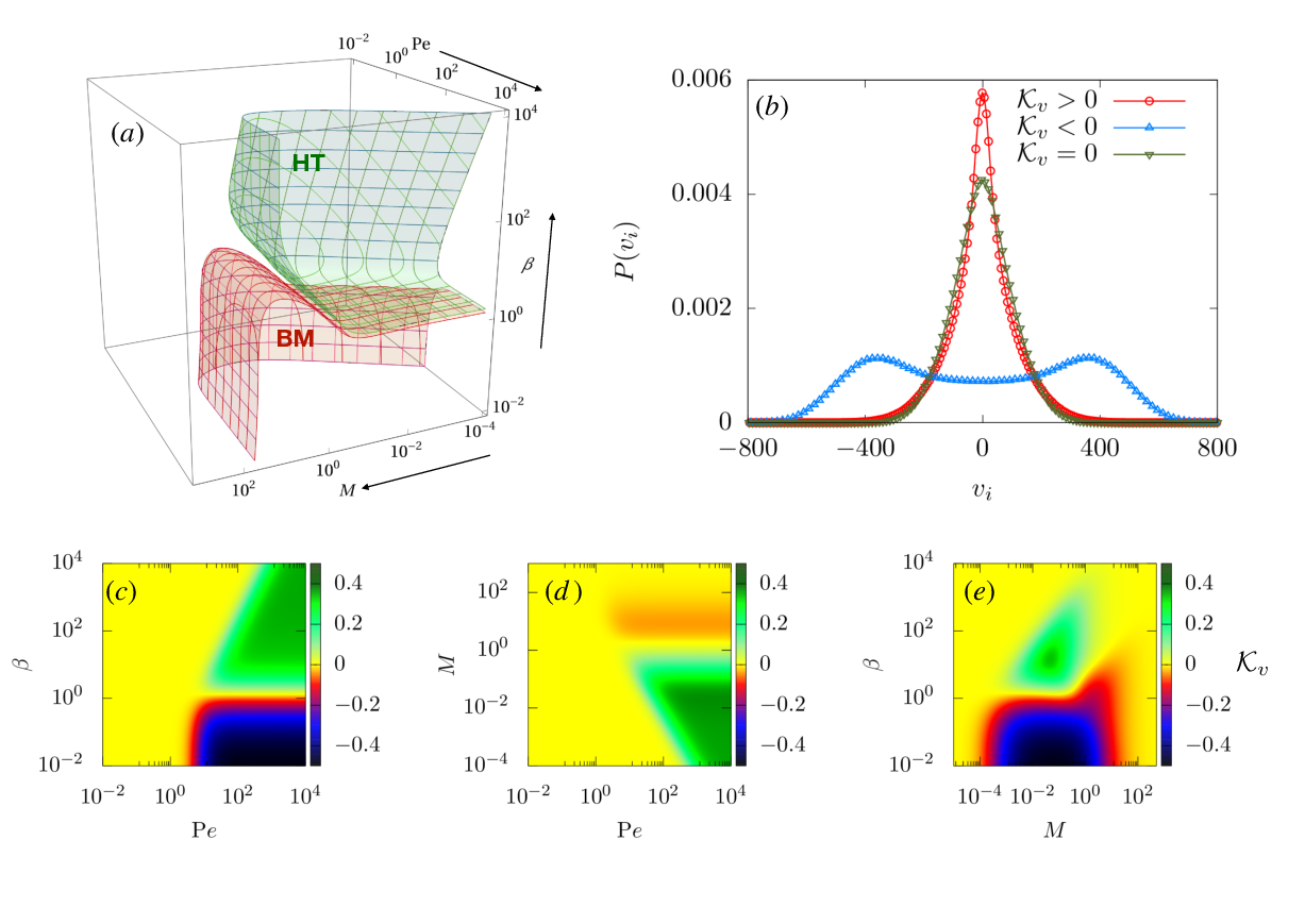
Figure 6: ‘Phase diagram’ and distribution in velocity for 2d iABP: ($a$) ‘Phase diagram’ as a function of $M,{\rm Pe}$, and $\beta$. Regions of bimodal (BM) and heavy-tailed-unimodal (HT) distributions of velocity components are identified using fixed kurtosis surfaces ${\cal K}_{v}=-0.03$ (red) and ${\cal K}_{v}=0.01$ (green). ($b$) Marginal distributions of velocity components $P(v_{i})$ with $v_{i}=v_{x}$ or $v_{y}$ obtained from numerical simulations. The parameter value for ${\cal K}_{v}>0$ are $M=0.01$, $\beta=10$, ${\rm Pe}=500$; for ${\cal K}_{v}<0$ are $M=0.01$, $\beta=0.1$, ${\rm Pe}=500$; and for ${\cal K}_{v}=0$ are $M=1$, $\beta=10$, ${\rm Pe}=500$. The ‘phase diagrams’ are further illustrated using heat-maps of ${\cal K}_{v}$ in $\beta-{\rm Pe}$ plane at $M=0.1$ ($c$), in $M-{\rm Pe}$ plane at $\beta=10$ ($d$), and in $\beta-M$ plane at ${\rm Pe}=100$ ($e$). Plots of kurtosis use equation (37).

At small $\beta$, ${\cal K}_{v}$ starts from ${\cal K}_{v}=-\{M^{2}{\rm Pe}^{4}(3+7M)\}/[2(3+M)(1+2M)(2+M(2+{\rm Pe}^{2}))^{2}]$ in 2d, a value same as for free iABPs. It varies non-monotonically at intermediate $\beta$ to vanish at large trap strength as ${\cal K}_{v}\approx\beta^{-2}\,(M^{2}{\rm Pe}^{4})/(8+32M)$ in 2d. ${\cal K}_{v}$ shows a non-monotonic behavior with $M$ as well and vanishes in the two limits of small and large inertia. In the limit of $M\to 0$, it vanishes as ${\cal K}_{v}\approx M^{2}\,\{[-2+3(-1+\beta)\beta]{\rm Pe}^{4}\}/[8(1+\beta)^{2}(2+\beta)(1+3\beta)]$ and in the other limit of $M\to\infty$, it vanishes as ${\cal K}_{v}\approx-M^{-1}\times 21{\rm Pe}^{4}/[16(2+{\rm Pe}^{2})^{2}]$ in 2d. With activity ${\rm Pe}$, ${\cal K}_{v}$ vanishes as $\sim{\rm Pe}^{4}$ in the small activity limit ${\rm Pe}\to 0$. With increasing ${\rm Pe}$ it shows non-equilibrium departures to saturate to either positive or negative values at high enough ${\rm Pe}$.

This velocity kurtosis is used to obtain a “phase diagram” in the three-dimensional parameter space of activity ${\rm Pe}$, trap stiffness $\beta$ and inertia $M$ (see figure 6($a$) ). We plot equi-kurtosis planes of positive and negative values, ${\cal K}_{v}=0.01$ (green plane) and ${\cal K}_{v}=-0.03$ (red plane) to identify different kinds of non-Gaussian departures. The region above the positive kurtosis plane ${\cal K}_{v}=0.01$ is denoted HT in the figure to indicate parameter regimes in which heavy-tailed marginal distributions of velocity components are observed, as shown in figure 6($b$). Similarly, the region below the ${\cal K}_{v}=-0.03$ plane is denoted BM to indicate the bimodal marginal distributions of velocity components for the corresponding parameter values, as shown in figure 6($b$). This BM distribution corresponds to an inverted wine bottle or Mexican hat shape for the velocity vector distribution in 2d. To further clarify the phase behavior, we plot two-dimensional projections of the phase diagram using heat-maps of kurtosis values in the ${\rm Pe}-\beta$, ${\rm Pe}-M$, and $M-\beta$ planes in figures 6($c$)-($e$), respectively. The yellow regions in the figures denote nearly Gaussian distributions of vanishing kurtosis, while the dark blue and green regions stand for negative and positive kurtosis, respectively. A thin region of vanishing kurtosis persists even for large ${\rm Pe}$, balanced by $\beta$ and $M$. At small $\beta$, the kurtosis ${\cal K}_{v}\leq 0$, as shown in figure 6($c$) and (e). These figures also show that for sufficiently large $\beta$, ${\cal K}_{v}$ can become positive. For a given $\beta$ and ${\rm Pe}$, it is possible to encounter re-entrant transition from Gaussian to a specific kind of non-Gaussian with positive or negative kurtosis to Gaussian with increasing $M$, as can be seen from figure 6($e$).

5.2.2 Kurtosis in displacement:

Again, we use equation (36) with $\bm{\phi}={\mathbf{r}}$ and $\langle{\mathbf{r}}^{4}\rangle_{\rm st}$ from equation (35) to get the kurtosis of displacement at steady state in 2d (see B for results in $d=3$ dimensions)

$${\cal K}_{r}=\frac{-\beta{\rm Pe}^{4}}{{\cal B}_{2}\left[2\beta+(1+M)(2+{\rm Pe}^{2})\right]^{2}}\left[\left\{21(1+M)^{3}(2+M)(3+M)(1+2M)(1+4M)\right\}\right.$$

$$\left.+\beta\left\{2(1+M)(27+M(291+M(1315+M(3061+14M(218+53M)))))\right\}+\beta^{2}\left\{M(99\right.\right.$$

$$\left.\left.+M(786+M(2053+2M(783-128M))))\right\}-36\beta^{3}M^{2}\left\{-1+(M-6)M\right\}\right],$$ (38)

where, ${\cal B}_{2}$ has the same expression as the one given after equation (37). It is easy to check that the expression for displacement kurtosis reduces to the known results for overdamped ABPs in a harmonic trap [52] in the limit of $M\to 0$.

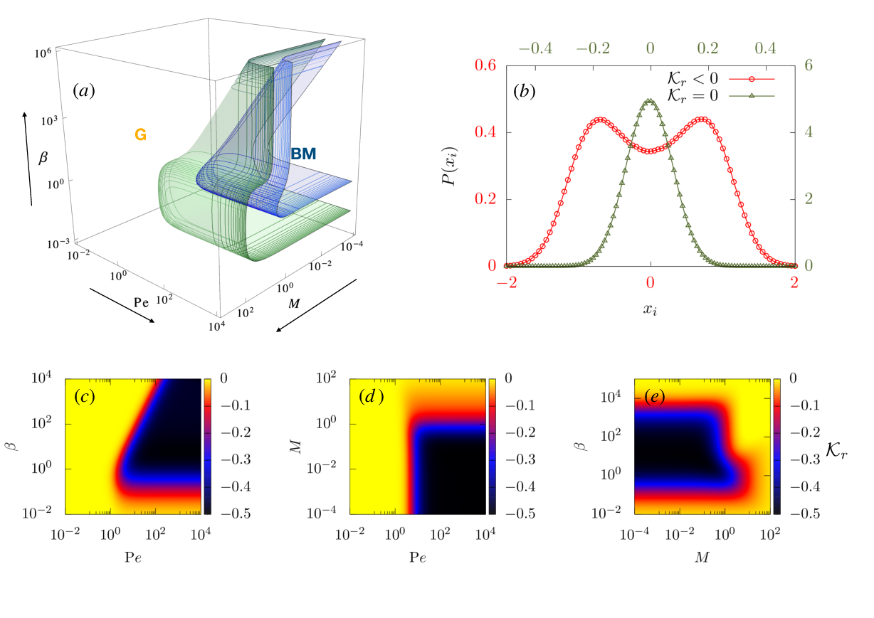
Figure 7: ‘Phase diagram’ and distribution in displacement for 2d iABP: ($a$) ‘Phase diagram’ as a function of $M,{\rm Pe}$, and $\beta$. Regions of Gaussian (G) and bimodal (BM) distributions of displacement components are identified using fixed kurtosis surfaces for ${\cal K}_{r}=-0.02$ (in green) and ${\cal K}_{r}=-0.3$ (in blue). ($b$) The simulated probability distribution of displacements $x_{i}=x$ or $y$ obtained from numerical simulations. The points are the simulation results, and the lines are guides to the eye. The bimodal distribution at ${\cal K}_{r}<0$ corresponds to $M=0.1$, $\beta=10$, ${\rm Pe}=10$ and the Gaussian distribution at ${\cal K}_{r}=0$ corresponds to $M=0.1$, $\beta=200$, ${\rm Pe}=10$. ($c$) – ($e$) shows heat-maps of kurtosis ${\cal K}_{r}$ across three planar sections of ($a$), in $\beta-{\rm Pe}$ plane with $M=0.1$ ($c$), in $M-{\rm Pe}$ plane with $\beta=10$ ($d$), and in $\beta-M$ plane with ${\rm Pe}=100$ ($e$). Plots of kurtosis ${\cal K}_{r}$ uses equation (38).

For vanishing $M$, kurtosis of displacement saturates to ${\cal K}_{r}=-\{\beta{\rm Pe}^{4}(7+3\beta)\}/[2(2+\beta)(1+3\beta)(2+2\beta+{\rm Pe}^{2})^{2}]$ in 2d, a negative value that describes overdamped ABPs in a harmonic trap [52]. It increases monotonically with $M$ to vanish as ${\cal K}_{r}\approx-M^{-1}\times 21{\rm Pe}^{4}/[16(2+{\rm Pe}^{2})^{2}]$ in the limit $M\to\infty$. With activity, ${\cal K}_{r}$ vanishes as ${\cal K}_{r}\sim-{\rm Pe}^{4}$ as ${\rm Pe}$ vaishes. It becomes negative with increasing activity to saturate to $M$ and $\beta$ dependent values. With trap strength, ${\cal K}_{r}$ vanishes in the two limits of small and large $\beta$. In the limit $\beta\to 0$, it vanishes linearly as ${\cal K}_{r}\approx-\beta\times 7{\rm Pe}^{4}/[4(2+{\rm Pe}^{2})^{2}]$. On the other hand, in the limit $\beta\to\infty$, it vanishes as $\beta^{-2}\times[(-1+M(M-6)){\rm Pe}^{4}]/[(8+32M)]$.

The displacement kurtosis is used to obtain a “phase diagram” in the three-dimensional parameter space of activity ${\rm Pe}$, trap stiffness $\beta$ and inertia $M$ (see figure 7($a$) ). Here, we plot equi-kurtosis planes of two different negative values, ${\cal K}_{r}=-0.02$ (green plane) and ${\cal K}_{r}=-0.3$ (blue plane) to identify different degrees of non-Gaussian departures. Note that unlike ${\cal K}_{v}$, ${\cal K}_{r}$ is never positive. The region to the left of the negative kurtosis plane ${\cal K}_{r}=-0.02$ is denoted G in the figure to indicate parameter regimes in which Gaussian distributions of displacement of vanishing kurtosis are observed, as shown in figure 7($b$). Similarly, the region to the right of the ${\cal K}_{r}=-0.3$ plane is denoted BM to indicate the bimodal marginal distributions of displacement components for the corresponding parameter values, as shown in figure 7($b$). To further clarify the phase behavior, we plot three two-dimensional projections of the phase diagram using heat-maps of kurtosis values in the ${\rm Pe}-\beta$, ${\rm Pe}-M$, and $M-\beta$ planes in figures 7($c$)-($e$), respectively. The yellow regions in the figures denote nearly Gaussian distributions of vanishing kurtosis, while the dark blue regions stand for negative kurtosis. At a given $M$, a re-entrant transition from Gaussian to BM to Gaussian can be obtained by increasing $\beta$, as can be seen in figures 7($c$) and ($e$). While ${\rm Pe}$ drives the displacement to non-equilibrium BM distributions, large $M$ moves it back towards equilibrium-like Gaussian distributions.

The position phase diagrams also suggest a method for particle segregation in active matter using a trap. The differential accumulation of iABPs with small activity near the trap center and that with high activity at the boundary can be utilized to segregate these two kinds of particles. More interesting is the inertia dependence. In the presence of intermediate trap strength, particles with large $M$ accumulate near the trap center, and those with small $M$ near the trap boundary, allowing for a method of segregating massive and lighter iABPs.

6 Outlook

In conclusion, we presented an exact method to calculate all the time-dependent dynamical moments of $d$-dimensional iABPs in a harmonic trap. We derived the time evolution of several dynamical moments, including the second and fourth moments of velocity and displacement, to observe excellent agreement with numerical simulations. Remarkably, the steady-state kinetic temperature and an estimate of effective diffusivity depend on inertia and trap stiffness, with inertial dependence of the diffusivity entering through the potential. This suggests a possible inertia-dependence of diffusivity in a system of interacting iABPs, as has been observed in recent numerical simulations [56].

While the non-equilibrium activity drives the steady-state distributions of velocity and displacement away from the equilibrium Gaussian, large inertia and trap strength suppress non-Gaussian fluctuations to bring back equilibrium-like features. These behaviors are quantified using the exact expressions for excess kurtosis in velocity and displacement. We presented detailed ‘phase diagrams’ using them for three control parameters: inertia, trap strength, and activity. The position phase diagram suggests a method using harmonic traps to segregate particles based on their activity and inertia.

The excess velocity kurtosis showed both negative and positive departures associated with distributions of velocity components being bimodal and heavy-tailed-unimodal, respectively. Further, the velocity kurtosis displays non-monotonic variation with $M$, indicating the possibility of a ‘re-entrant transition’ from Gaussian to non-Gaussian to Gaussian. Our exact expression for kurtosis of displacement revealed a qualitatively different ‘phase diagram’. It showed two ‘phases’, one with a negative value associated with the ‘active’ bimodal distribution corresponding to particle accumulation near the boundary and the other with a vanishing value for the ‘passive’ Gaussian phase corresponding to predominant particle accumulation near trap center. A non-monotonicity and re-entrant ‘transition’ is observed for displacement kurtosis as well, with increasing $\beta$ but not with $M$.

Experiment	$m(g)$	$v_{0}(cm/s)$	$\gamma\equiv\frac{1}{\mu}(g/s)$	$k(g/s^{2})$	$D(cm^{2}/s)$	$D_{r}(s^{-1})$
vibrobot [18]	$0.33-4.07$	$5.7-9.3$	$\sim 1.65-26.3$	$-$	$0.36-2.2$	$0.59-2.7$
hexbugs [60]	$7.5$	$10$	$\sim 10.9-54.8$	$\sim 80.2$	$-$	$\sim 0.006-0.06$
hexbugs [61]	$7.2$	$13$	$\sim 720$	$90$	$-$	$0.3$

Table 1: Estimate of experimentally achieved parameter range.

The analytical predictions in our study are amenable to direct experimental verifications. For example, we consider recent experiments on vibrobots [18] and hexbugs [60] to extract relevant parameter values and compare them with the dimensionless parameter regimes used in this paper. Some of these experiments used the parabolic dish to generate an effective harmonic trapping [60, 61], where the trap-strength $k$ is determined by the geometry of the dish and gravity, using $kr^{2}/2=mgh$ where $m$ is the mass of the active particle, $g$ is the gravitational acceleration, and $h$ is the maximum height of the dish of radius $r$. We list the parameter values estimated from Ref. [18, 61, 60] in Table-1. Wherever a required measure is not available explicitly, we use the values supplied in other related experiments; e.g., for effective translational diffusivity, we use $D\sim 1\,{\rm cm}^{2}/{\rm s}$ for both vibrobots and hexbugs (see Table-2). This is a value within the range measured in Ref. [18]. Using this approach, we report the estimated dimensionless parameters in Table-2. The numbers realized, $M\sim 0.001-20$, ${\rm Pe}\sim 1-130$, and $\beta\sim 0.1-250$, span a broad enough range to cover approximately all the different velocity and displacement phases we predicted. Further, the parameter values used in figures 1, 2, 4 lie within the range estimated in this table. Similar experiments can be used to test our predictions for transitions between active and passive behaviors.

Experiment	$M$	${\rm Pe}$	$\beta$
vibrobot [18]	$\sim 1.77-18.5$	$\sim 4.01-12.5$	$-$
hexbugs [60]	$\sim 0.0008-0.04$	$\sim 40.8-129$	$\sim 24.34-243.4$
hexbugs [61]	$\sim 0.003$	$\sim 23$	$\sim 0.42$

Table 2: Estimate of dimensionless parameter values obtained from experiments. For hexbugs of similar sizes as vibrobots, we use $D=1\,\rm{cm}^{2}/\rm{s}$, picked from the range of measured vibrobot diffusivities [18].

Appendix A Fourth moment of velocity and position

The calculation of $\langle{\mathbf{v}}^{4}\rangle_{s}$ and $\langle{\mathbf{r}}^{4}\rangle_{s}$ utilises equation (6) and follows the following steps:

$$(i)\,s\langle{\mathbf{r}}^{4}\rangle_{s}={\mathbf{r}}_{0}^{4}+4\langle({\mathbf{v}}\cdot{\mathbf{r}}){\mathbf{r}}^{2}\rangle_{s},$$ (39)

$$(ii)\,(s+1/M)\langle({\mathbf{v}}\cdot{\mathbf{r}}){\mathbf{r}}^{2}\rangle_{s}=({\mathbf{v}}_{0}\cdot{\mathbf{r}}_{0}){\mathbf{r}}_{0}^{2}+\langle{\mathbf{v}}^{2}{\mathbf{r}}^{2}\rangle_{s}+2\langle({\mathbf{v}}\cdot{\mathbf{r}})^{2}\rangle_{s}+{\rm Pe}\langle(\hat{\bm{u}}\cdot{\mathbf{r}}){\mathbf{r}}^{2}\rangle_{s}/M$$

$$-\beta\langle{\mathbf{r}}^{4}\rangle_{s}/M,$$ (40)

$$(iii)\,(s+2/M)\langle{\mathbf{v}}^{2}{\mathbf{r}}^{2}\rangle_{s}={\mathbf{v}}_{0}^{2}{\mathbf{r}}_{0}^{2}+2\langle({\mathbf{v}}\cdot{\mathbf{r}}){\mathbf{v}}^{2}\rangle_{s}+2{\rm Pe}\langle(\hat{\bm{u}}\cdot{\mathbf{v}}){\mathbf{r}}^{2}\rangle_{s}/M-2\beta\langle({\mathbf{v}}\cdot{\mathbf{r}}){\mathbf{r}}^{2}\rangle_{s}/M$$

$$+2d\langle{\mathbf{r}}^{2}\rangle_{s}/M^{2},$$ (41)

$$(iv)\,(s+3/M)\langle({\mathbf{v}}\cdot{\mathbf{r}}){\mathbf{v}}^{2}\rangle_{s}=({\mathbf{v}}_{0}\cdot{\mathbf{r}}_{0}){\mathbf{v}}_{0}^{2}+\langle{\mathbf{v}}^{4}\rangle_{s}+{\rm Pe}\langle(\hat{\bm{u}}\cdot{\mathbf{r}}){\mathbf{v}}^{2}\rangle_{s}/M+2{\rm Pe}\langle(\hat{\bm{u}}\cdot{\mathbf{v}})({\mathbf{v}}\cdot{\mathbf{r}})\rangle_{s}/M$$

$$-\beta\langle{\mathbf{v}}^{2}{\mathbf{r}}^{2}\rangle_{s}/M-2\beta\langle({\mathbf{v}}\cdot{\mathbf{r}})^{2}\rangle_{s}/M+2(d+2)\langle{\mathbf{v}}\cdot{\mathbf{r}}\rangle_{s}/M^{2},$$ (42)

$$(v)\,[s+2/M+(d-1)]\langle(\hat{\bm{u}}\cdot{\mathbf{v}})({\mathbf{v}}\cdot{\mathbf{r}})\rangle_{s}=(\hat{\bm{u}}_{0}\cdot{\mathbf{v}}_{0})({\mathbf{v}}_{0}\cdot{\mathbf{r}}_{0})+\langle(\hat{\bm{u}}\cdot{\mathbf{v}}){\mathbf{v}}^{2}\rangle_{s}+{\rm Pe}\langle{\mathbf{v}}\cdot{\mathbf{r}}\rangle_{s}/M$$

$$+{\rm Pe}\langle(\hat{\bm{u}}\cdot{\mathbf{v}})(\hat{\bm{u}}\cdot{\mathbf{r}})\rangle_{s}/M-\beta\langle(\hat{\bm{u}}\cdot{\mathbf{r}})({\mathbf{v}}\cdot{\mathbf{r}})\rangle_{s}/M-\beta\langle(\hat{\bm{u}}\cdot{\mathbf{v}}){\mathbf{r}}^{2}\rangle_{s}/M+2\langle\hat{\bm{u}}\cdot{\mathbf{r}}\rangle_{s}/M^{2},$$ (43)

$$(vi)\,[s+3/M+(d-1)]\langle(\hat{\bm{u}}\cdot{\mathbf{v}}){\mathbf{v}}^{2}\rangle_{s}=(\hat{\bm{u}}_{0}\cdot{\mathbf{v}}_{0}){\mathbf{v}}_{0}^{2}+{\rm Pe}\langle{\mathbf{v}}^{2}\rangle_{s}/M+2{\rm Pe}\langle(\hat{\bm{u}}\cdot{\mathbf{v}})^{2}\rangle_{s}/M$$

$$-\beta\langle(\hat{\bm{u}}\cdot{\mathbf{r}}){\mathbf{v}}^{2}\rangle_{s}/M-2\beta\langle(\hat{\bm{u}}\cdot{\mathbf{v}})({\mathbf{v}}\cdot{\mathbf{r}})\rangle_{s}/M+2(d+2)\langle(\hat{\bm{u}}\cdot{\mathbf{v}})\rangle_{s}/M^{2},$$ (44)

$$(vii)\,[s+2/M+2d]\langle(\hat{\bm{u}}\cdot{\mathbf{v}})^{2}\rangle_{s}=(\hat{\bm{u}}_{0}\cdot{\mathbf{v}}_{0})^{2}+2{\rm Pe}\langle(\hat{\bm{u}}\cdot{\mathbf{v}})\rangle_{s}/M-2\beta\langle(\hat{\bm{u}}\cdot{\mathbf{v}})(\hat{\bm{u}}\cdot{\mathbf{r}})\rangle_{s}/M$$

$$+2/(sM^{2})+2\langle{\mathbf{v}}^{2}\rangle_{s},$$ (45)

$$(viii)\,[s+2/M+(d-1)]\langle(\hat{\bm{u}}\cdot{\mathbf{r}}){\mathbf{v}}^{2}\rangle_{s}=(\hat{\bm{u}}_{0}\cdot{\mathbf{r}}_{0}){\mathbf{v}}_{0}^{2}+\langle(\hat{\bm{u}}\cdot{\mathbf{v}}){\mathbf{v}}^{2}\rangle_{s}+2{\rm Pe}\langle(\hat{\bm{u}}\cdot{\mathbf{v}})(\hat{\bm{u}}\cdot{\mathbf{r}})\rangle_{s}/M$$

$$-2\beta\langle(\hat{\bm{u}}\cdot{\mathbf{r}})({\mathbf{v}}\cdot{\mathbf{r}})\rangle_{s}/M+2d\langle(\hat{\bm{u}}\cdot{\mathbf{r}})\rangle_{s}/M^{2},$$ (46)

$$(ix)\,[s+1/M+2d]\langle(\hat{\bm{u}}\cdot{\mathbf{v}})(\hat{\bm{u}}\cdot{\mathbf{r}})\rangle_{s}=(\hat{\bm{u}}_{0}\cdot{\mathbf{v}}_{0})(\hat{\bm{u}}_{0}\cdot{\mathbf{r}}_{0})+\langle(\hat{\bm{u}}\cdot{\mathbf{v}})^{2}\rangle_{s}+{\rm Pe}\langle(\hat{\bm{u}}\cdot{\mathbf{r}})\rangle_{s}/M$$

$$-\beta\langle(\hat{\bm{u}}\cdot{\mathbf{r}})^{2}\rangle_{s}/M+2\langle({\mathbf{v}}\cdot{\mathbf{r}})\rangle_{s},$$ (47)

$$(x)\,[s+1/M+(d-1)]\langle(\hat{\bm{u}}\cdot{\mathbf{v}}){\mathbf{r}}^{2}\rangle_{s}=(\hat{\bm{u}}_{0}\cdot{\mathbf{v}}_{0}){\mathbf{r}}_{0}^{2}+2\langle(\hat{\bm{u}}\cdot{\mathbf{v}})({\mathbf{v}}\cdot{\mathbf{r}})\rangle_{s}+{\rm Pe}\langle{\mathbf{r}}^{2}\rangle_{s}/M$$

$$-\beta\langle(\hat{\bm{u}}\cdot{\mathbf{r}}){\mathbf{r}}^{2}\rangle_{s}/M,$$ (48)

$$(xi)\,(s+2/M)\langle({\mathbf{v}}\cdot{\mathbf{r}})^{2}\rangle_{s}=({\mathbf{v}}_{0}\cdot{\mathbf{r}}_{0})^{2}+2\langle({\mathbf{v}}\cdot{\mathbf{r}}){\mathbf{v}}^{2}\rangle_{s}+2{\rm Pe}\langle(\hat{\bm{u}}\cdot{\mathbf{r}})({\mathbf{v}}\cdot{\mathbf{r}})\rangle_{s}/M$$

$$-2\beta\langle({\mathbf{v}}\cdot{\mathbf{r}}){\mathbf{r}}^{2}\rangle_{s}/M+2\langle{\mathbf{r}}^{2}\rangle_{s}/M^{2},$$ (49)

$$(xii)\,[s+(d-1)]\langle(\hat{\bm{u}}\cdot{\mathbf{r}}){\mathbf{r}}^{2}\rangle_{s}=(\hat{\bm{u}}_{0}\cdot{\mathbf{r}}_{0}){\mathbf{r}}_{0}^{2}+\langle(\hat{\bm{u}}\cdot{\mathbf{v}}){\mathbf{r}}^{2}\rangle_{s}+2\langle(\hat{\bm{u}}\cdot{\mathbf{r}})({\mathbf{v}}\cdot{\mathbf{r}})\rangle_{s},$$ (50)

$$(xiii)\,(s+4/M)\langle{\mathbf{v}}^{4}\rangle_{s}={\mathbf{v}}_{0}^{4}+4{\rm Pe}\langle(\hat{\bm{u}}\cdot{\mathbf{v}}){\mathbf{v}}^{2}\rangle_{s}/M-4\beta\langle({\mathbf{v}}\cdot{\mathbf{r}}){\mathbf{v}}^{2}\rangle_{s}/M$$

$$+4(d+2)\langle{\mathbf{v}}^{2}\rangle_{s}/M,$$ (51)

$$(xiv)\,[s+1/M+(d-1)]\langle(\hat{\bm{u}}\cdot{\mathbf{r}})({\mathbf{v}}\cdot{\mathbf{r}})\rangle_{s}=(\hat{\bm{u}}_{0}\cdot{\mathbf{r}}_{0})({\mathbf{v}}_{0}\cdot{\mathbf{r}}_{0})+\langle(\hat{\bm{u}}\cdot{\mathbf{v}})({\mathbf{v}}\cdot{\mathbf{r}})\rangle_{s}+$$

$$\langle(\hat{\bm{u}}\cdot{\mathbf{r}}){\mathbf{v}}^{2}\rangle_{s}+{\rm Pe}\langle(\hat{\bm{u}}\cdot{\mathbf{r}})^{2}\rangle_{s}/M-\beta\langle(\hat{\bm{u}}\cdot{\mathbf{r}}){\mathbf{r}}^{2}\rangle_{s}/M,$$ (52)

$$(xv)\,(s+2d)\langle(\hat{\bm{u}}\cdot{\mathbf{r}})^{2}\rangle_{s}=(\hat{\bm{u}}_{0}\cdot{\mathbf{r}}_{0})^{2}+2\langle(\hat{\bm{u}}\cdot{\mathbf{v}})(\hat{\bm{u}}\cdot{\mathbf{r}})\rangle_{s}+2\langle{\mathbf{r}}^{2}\rangle_{s}.$$ (53)

where $\langle\hat{\bm{u}}\cdot{\mathbf{r}}\rangle_{s}=\langle r_{\parallel}\rangle_{s}$, $\langle{\mathbf{v}}\cdot{\mathbf{r}}\rangle_{s}$, $\langle\hat{\bm{u}}\cdot{\mathbf{v}}\rangle_{s}=\langle v_{\parallel}\rangle_{s}$, $\langle{\mathbf{r}}^{2}\rangle_{s}$, and $\langle{\mathbf{v}}^{2}\rangle_{s}$ were already calculate in equations (13), (18), (12), (19), and (17) respectively. Solving these coupled equations, one can get the fourth-order moments in the Laplace space such as $\langle{\mathbf{r}}^{4}\rangle_{s}$ and $\langle{\mathbf{v}}^{4}\rangle_{s}$ and the inverse Laplace transform can be used to get the full-time evolution.

Appendix B Kurtosis and fourth moments in $d=3$ dimensions

Solving equations (39) $-$ (53) for $\langle{\mathbf{r}}^{4}\rangle_{s}$ and $\langle{\mathbf{v}}^{4}\rangle_{s}$ and taking the inverse Laplace transform, we get the full-time evolution in arbitrary dimension. We expand these expressions around $t=0$ for initial values ${\mathbf{r}}_{0}=\bf{0}$ and ${\mathbf{v}}_{0}=\bf{0}$ in $d=3$ dimensions to get

$$\langle{\mathbf{v}}^{4}\rangle(t)=\frac{60}{M^{4}}t^{2}+\frac{20(M{\rm Pe}^{2}-6)}{M^{5}}t^{3}$$

$$+\frac{[420+M\{-120\beta-40(M+3){\rm Pe}^{2}+3M{\rm Pe}^{4}\}]}{3M^{6}}t^{4}+{\cal O}(t^{5}),$$ (54)

$$\langle{\mathbf{r}}^{4}\rangle(t)=\frac{20}{3M^{4}}t^{6}+\frac{5(M{\rm Pe}^{2}-6)}{3M^{5}}t^{7}$$

$$+\frac{[1212+M\{-384\beta-4(32M+85){\rm Pe}^{2}+9M{\rm Pe}^{4}\}]}{144M^{6}}t^{8}+{\cal O}(t^{9}).$$ (55)

The comparison of equations (B) and (B) with the equations (32) and (5.1) respectively suggests that the nature of crossover in the dynamic is independent of dimensions. However, the crossover time itself depends on the dimensions.

In the asymptotic limit of a long time, we get the steady-state results in $d=3$ dimensions as

$$\langle{\mathbf{v}}^{4}\rangle_{\rm st}=\frac{15}{M^{2}}+\frac{20}{M(2+\beta+4M)}{\rm Pe}^{2}+\frac{4\,{\cal A}_{3}}{{\cal B}_{3}}{\rm Pe}^{4},$$ (56)

where ${\cal A}_{3}=\{18(1+M)(1+2M)(3+5M)(1+6M)+3\beta[36+M(423+M(1495+2M(1021+12M(49+20M))))]+\beta^{2}M[198+M(1371+50M(67+68M))]+72\beta^{3}M^{2}(1+5M)\}$ and ${\cal B}_{3}=\{(2+\beta+4M)(6+9\beta+4M)(1+6M)(3+\beta+9M)(3+4\beta M)(2+M(6+\beta+4M))\}$.

Further,

$$\langle{\mathbf{r}}^{4}\rangle_{\rm st}=\frac{15}{\beta^{2}}+\frac{10(2M+1)}{\beta^{2}(2+\beta+4M)}{\rm Pe}^{2}+\frac{{\cal A}_{4}}{\beta^{2}{\cal B}_{3}}{\rm Pe}^{4},$$ (57)

where ${\cal A}_{4}=\{30(1+M)(1+2M)^{2}(3+2M)(1+3M)(1+6M)+\beta[(1+2M)(1+6M)(54+M(435+M(1325+2M(885+4M(167+60M)))))]+\beta^{2}M[99+2M(633+10M(311+M(881+10M(135+68M))))]+36\beta^{3}M^{2}[1+2M(5+4M(6+5M))]\}$. The limiting behavior of $\langle{\mathbf{v}}^{4}\rangle_{\rm st}$ and $\langle{\mathbf{r}}^{4}\rangle_{\rm st}$ with $M$ and $\beta$ in $d=3$ dimensions shows the same qualitative feature as in 2d.

Following the definition of kurtosis from equation (36) and the steady state results from this section for $d=3$ dimensions, we write the kurtosis of velocity and displacement in $d=3$ dimensions as

$${\cal K}_{v}=\frac{-4M^{2}{\rm Pe}^{4}}{{\cal B}_{4}}\left[\left\{72(1+M)(1+2M)(1+6M)(3+11M)\right\}+\beta\left\{12(15+M(151+4M(139\right.\right.$$

$$\left.\left.+M(230+M(215+198M)))))\right\}+\beta^{2}\left\{-54+2M(-375+2M(307+4110M+5324M^{2}))\right\}\right.$$

$$\left.+\beta^{3}M(-99+M(165-214M))-36M^{2}\beta^{4}\right],$$ (58)

where ${\cal B}_{4}=5(6+9\beta+4M)(1+6M)(3+\beta+9M)(3+4\beta M)(2+M(6+\beta+4M))(6+3\beta+2M(6+{\rm Pe}^{2}))^{2}$,

and

$${\cal K}_{r}=\frac{-2\beta{\rm Pe}^{4}}{{\cal B}_{5}}\left[\left\{66(1+M)(1+2M)^{3}(3+2M)(1+3M)(1+6M)\right\}+\beta\left\{(1+2M)(54\right.\right.$$

$$\left.\left.+M(957+M(7187+2M(13865+88M(266+121M)))))\right\}+\beta^{2}\left\{M(99+2M(669\right.\right.$$

$$\left.\left.+M(3107+M(4313-214M))))\right\}-36M^{2}\beta^{3}\left\{-1+2M(M-5)\right\}\right],$$ (59)

where ${\cal B}_{5}=5(6+9\beta+4M)(1+6M)(3+\beta+9M)(3+4\beta M)(2+M(6+\beta+4M))[3\beta+(1+2M)(6+{\rm Pe}^{2})]^{2}$.

The kurtosis of velocity and position shows the same qualitative features in 3 dimensions as in for 2d; however, the boundary separating the different ‘phases’ gets shifted.

References

References

- [1] Clemens Bechinger, Roberto Di Leonardo, Hartmut Löwen, Charles Reichhardt, Giorgio Volpe, and Giovanni Volpe. Active Particles in Complex and Crowded Environments. Rev. Mod. Phys., 88(4):045006, nov 2016.
- [2] M. C. Marchetti, J. F. Joanny, S. Ramaswamy, T. B. Liverpool, J. Prost, Madan Rao, and R. Aditi Simha. Hydrodynamics of soft active matter. Rev. Mod. Phys., 85(3):1143–1189, jul 2013.
- [3] P Romanczuk, M Bär, W Ebeling, B. Lindner, and L. Schimansky-Geier. Active Brownian particles. Eur. Phys. J. Spec. Top., 202(1):1–162, mar 2012.
- [4] Sriram Ramaswamy. Active fluids. Nat. Rev. Phys., 1(11):640–642, oct 2019.
- [5] R. D. Astumian and P. Hänggi. Brownian Motors. Physics Today, 55(11):33–40, November 2002.
- [6] Peter Reimann. Brownian motors: Noisy transport far from equilibrium. Physics Report, 361(2-4):57–265, apr 2002.
- [7] Howard C. Berg and Douglas A. Brown. Chemotaxis in Escherichia coli analysed by three-dimensional tracking. Nature, 239(5374):500–504, 1972.
- [8] Hiro Sato Niwa. Self-organizing dynamic model of fish schooling. Journal of Theoretical Biology, 171(2):123–136, nov 1994.
- [9] Francesco Ginelli, Fernando Peruani, Marie-Helène Pillot, Hugues Chaté, Guy Theraulaz, and Richard Bon. Intermittent collective dynamics emerge from conflicting imperatives in sheep herds. Proc. Natl. Acad. Sci., 112(41):12729–12734, oct 2015.
- [10] Harvey L. Devereux, Colin R. Twomey, Matthew S. Turner, and Shashi Thutupalli. Whirligig beetles as corralled active Brownian particles. J. R. Soc. Interface, 18(177), 2021.
- [11] Haripriya Mukundarajan, Thibaut C. Bardon, Dong Hyun Kim, and Manu Prakash. Surface tension dominates insect flight on fluid interfaces. J. Exp. Biol., 219(5):752–766, 2016.
- [12] Jean Rabault, Richard A. Fauli, and Andreas Carlson. Curving to Fly: Synthetic Adaptation Unveils Optimal Flight Performance of Whirling Fruits. Phys. Rev. Lett., 122(2):24501, 2019.
- [13] M E Cates and J Tailleur. When are active Brownian particles and run-and-tumble particles equivalent? Consequences for motility-induced phase separation. Europhys. Lett., (2):20010.
- [14] É. Fodor, C. Nardini, M. E. Cates, J. Tailleur, P. Visco, and F. van Wijland. How far from equilibrium is active matter? Phys. Rev. Lett., 117:038103, Jul 2016.
- [15] Shibananda Das, Gerhard Gompper, and Roland G. Winkler. Confined active Brownian particles: theoretical description of propulsion-induced accumulation. New J. Phys., 20(1):015001, jan 2018.
- [16] Amir Shee, Abhishek Dhar, and Debasish Chaudhuri. Active brownian particles: mapping to equilibrium polymers and exact computation of moments. Soft Matter, 16:4776–4787, 2020.
- [17] Christina Kurzthaler, Clémence Devailly, Jochen Arlt, Thomas Franosch, Wilson C. K. Poon, Vincent A. Martinez, and Aidan T. Brown. Probing the spatiotemporal dynamics of catalytic Janus particles with single-particle tracking and differential dynamic microscopy. Phys. Rev. Lett., 121:078001, Aug 2018.
- [18] Christian Scholz, Soudeh Jahanshahi, Anton Ldov, and Hartmut Löwen. Inertial delay of self-propelled particles. Nature Communications, 9(1), December 2018.
- [19] Vijay Narayan, Sriram Ramaswamy, Narayanan Menon, The Caspt, and The Caspt. Long-Lived Giant Number Fluctuations. Science (80-. )., 317(July):105–108, 2007.
- [20] Arshad Kudrolli, Geoffroy Lumay, Dmitri Volfson, and Lev S. Tsimring. Swarming and Swirling in Self-Propelled Polar Granular Rods. Phys. Rev. Lett., 100(5):058001, feb 2008.
- [21] Julien Deseigne, Olivier Dauchot, and Hugues Chaté. Collective Motion of Vibrated Polar Disks. Phys. Rev. Lett., 105(9):098001, aug 2010.
- [22] Nitin Kumar, Harsh Soni, Sriram Ramaswamy, and A. K. Sood. Flocking at a distance in active granular matter. Nat. Commun., 5(1):4688, dec 2014.
- [23] Lorenzo Caprini, Rahul Kumar Gupta, and Hartmut Löwen. Role of rotational inertia for collective phenomena in active matter. Phys. Chem. Chem. Phys., 24(40):24910–24916, 2022.
- [24] Somayeh Farhadi, Sergio Machaca, Justin Aird, Bryan O. Torres Maldonado, Stanley Davis, Paulo E. Arratia, and Douglas J. Durian. Dynamics and thermodynamics of air-driven active spinners. Soft Matter, 14(27):5588–5594, 2018.
- [25] Benjamin C. Van Zuiden, Jayson Paulose, William T.M. Irvine, Denis Bartolo, and Vincenzo Vitelli. Spatiotemporal order and emergent edge currents in active spinner materials. Proc. Natl. Acad. Sci. U. S. A., 113(46):12919–12924, 2016.
- [26] Lee Walsh, Caleb G. Wagner, Sarah Schlossberg, Christopher Olson, Aparna Baskaran, and Narayanan Menon. Noise and diffusion of a vibrated self-propelled granular particle. Soft Matter, 13:8964–8968, 2017.
- [27] Yaouen Fily and MC Marchetti. Athermal Phase Separation of Self-Propelled Particles with No Alignment. Phys. Rev. Lett., 108(June):235702, 2012.
- [28] Gabriel S. Redner, Michael F. Hagan, and Aparna Baskaran. Structure and Dynamics of a Phase-Separating Active Colloidal Fluid. Phys. Rev. Lett., 110(5):055701, jan 2013.
- [29] Claudio B. Caporusso, Pasquale Digregorio, Demian Levis, Leticia F. Cugliandolo, and Giuseppe Gonnella. Motility-Induced Microphase and Macrophase Separation in a Two-Dimensional Active Brownian Particle System. Phys. Rev. Lett., 125(17):178004, 2020.
- [30] Ahmad K. Omar, Katherine Klymko, Trevor GrandPre, Phillip L. Geissler, and John F. Brady. Tuning nonequilibrium phase transitions with inertia. The Journal of Chemical Physics, 158(7):074904, 02 2023.
- [31] Rayan Chatterjee, Navdeep Rana, R Aditi Simha, Prasad Perlekar, and Sriram Ramaswamy. Inertia drives a flocking phase transition in viscous active fluids. Physical Review X, 11(3):031063, 2021.
- [32] Michele Caraglio and Thomas Franosch. Analytic solution of an active brownian particle in a harmonic well. Phys. Rev. Lett., 129:158001, Oct 2022.
- [33] Urvashi Nakul and Manoj Gopalakrishnan. Stationary states of an active brownian particle in a harmonic trap. Phys. Rev. E, 108:024121, Aug 2023.
- [34] Kanaya Malakar, Arghya Das, Anupam Kundu, K. Vijay Kumar, and Abhishek Dhar. Steady state of an active brownian particle in a two-dimensional harmonic trap. Phys. Rev. E, 101:022610, Feb 2020.
- [35] Dan Wexler, Nir Gov, Kim Ø. Rasmussen, and Golan Bel. Dynamics and escape of active particles in a harmonic trap. Phys. Rev. Res., 2:013003, Jan 2020.
- [36] Marc Hennes, Katrin Wolff, and Holger Stark. Self-induced polar order of active brownian particles in a harmonic trap. Phys. Rev. Lett., 112:238104, Jun 2014.
- [37] Eric Woillez, Yariv Kafri, and Nir S. Gov. Active trap model. Phys. Rev. Lett., 124:118002, Mar 2020.
- [38] Urna Basu, Satya N Majumdar, Alberto Rosso, Sanjib Sabhapandit, and Grégory Schehr. Exact stationary state of a run-and-tumble particle with three internal states in a harmonic trap. Journal of Physics A: Mathematical and Theoretical, 53(9):09LT01, feb 2020.
- [39] Naftali R. Smith and Oded Farago. Nonequilibrium steady state for harmonically confined active particles. Phys. Rev. E, 106:054118, Nov 2022.
- [40] I. Buttinoni, L. Caprini, L. Alvarez, F. J. Schwarzendahl, and H. Löwen. Active colloids in harmonic optical potentials(a). Europhysics Letters, 140(2):27001, nov 2022.
- [41] Ion Santra, Urna Basu, and Sanjib Sabhapandit. Direction reversing active brownian particle in a harmonic potential. Soft Matter, 17:10108–10119, 2021.
- [42] Koushik Goswami. Heat fluctuation of a harmonically trapped particle in an active bath. Phys. Rev. E, 99:012112, Jan 2019.
- [43] Sho C. Takatori, Raf De Dier, Jan Vermant, and John F. Brady. Acoustic trapping of active matter. Nature Communications, 7(1):10694, 2016.
- [44] Luis L. Gutierrez-Martinez and Mario Sandoval. Inertial effects on trapped active matter. The Journal of Chemical Physics, 153(4):044906, 07 2020.
- [45] M. Muhsin and M. Sahoo. Inertial active ornstein-uhlenbeck particle in the presence of a magnetic field. Phys. Rev. E, 106:014605, Jul 2022.
- [46] G H Philipp Nguyen, René Wittmann, and Hartmut Löwen. Active ornstein–uhlenbeck model for self-propelled particles with inertia. Journal of Physics: Condensed Matter, 34(3):035101, nov 2021.
- [47] Lorenzo Caprini and Umberto Marini Bettolo Marconi. Inertial self-propelled particles. The Journal of Chemical Physics, 154(2):024902, 01 2021.
- [48] Angelica Arredondo, Catania Calavitta, Mauricio Gomez, Jose Mendez-Villanueva, Wylie W. Ahmed, and Nicholas D. Brubaker. Inertia suppresses signatures of activity of active brownian particles in a harmonic potential, 2023.
- [49] Derek Frydel. Active oscillator: Recurrence relation approach. Physics of Fluids, 36(1):011910, 01 2024.
- [50] Pamela Muñoz Obreque, Oscar Garrido, Diego Romero, Hartmut Löwen, and Francisca Guzmán-Lastra. Dynamics of magnetic self-propelled particles in a harmonic trap, 2024.
- [51] J. J. Hermans and R. Ullman. The statistics of stiff chains, with applications to light scattering. Physica, 18(11):951–971, November 1952.
- [52] Debasish Chaudhuri and Abhishek Dhar. Active brownian particle in harmonic trap: exact computation of moments, and re-entrant transition. Journal of Statistical Mechanics: Theory and Experiment, 2021(1):013207, jan 2021.
- [53] Amir Shee and Debasish Chaudhuri. Self-propulsion with speed and orientation fluctuation: Exact computation of moments and dynamical bistabilities in displacement. Phys. Rev. E, 105:054148, May 2022.
- [54] Amir Shee and Debasish Chaudhuri. Active brownian motion with speed fluctuations in arbitrary dimensions: exact calculation of moments and dynamical crossovers. Journal of Statistical Mechanics: Theory and Experiment, 2022(1):013201, jan 2022.
- [55] Manish Patel and Debasish Chaudhuri. Exact moments and re-entrant transitions in the inertial dynamics of active brownian particles. New Journal of Physics, 25(12):123048, dec 2023.
- [56] Shubhendu Shekhar Khali, Fernando Peruani, and Debasish Chaudhuri. When an active bath behaves as an equilibrium one. Phys. Rev. E, 109:024120, Feb 2024.
- [57] Kiyosi Itô. International Symposium on Mathematical Problems in Theoretical Physics, chapter Stochastic Calculus, pages 218–223. Springer-Verlag, Berlin-Heidelberg-New York, 1975.
- [58] M. van den Berg and J. T. Lewis. Brownian Motion on a Hypersurface. Bull. London Math. Soc., 17(2):144–150, mar 1985.
- [59] Aleksandar Mijatović, Veno Mramor, and Gerónimo Uribe Bravo. A note on the exact simulation of spherical Brownian motion. Stat. Probab. Lett., 165:108836, oct 2020.
- [60] Olivier Dauchot and Vincent Démery. Dynamics of a self-propelled particle in a harmonic trap. Phys. Rev. Lett., 122:068002, Feb 2019.
- [61] Cecilio Tapia-Ignacio, Luis L Gutierrez-Martinez, and Mario Sandoval. Trapped active toy robots: theory and experiment. Journal of Statistical Mechanics: Theory and Experiment, 2021(5):053404, may 2021.