HairFastGAN: Realistic and Robust Hair Transfer with a Fast Encoder-Based Approach

Abstract

Our paper addresses the complex task of transferring a hairstyle from a reference image to an input photo for virtual hair try-on. This task is challenging due to the need to adapt to various photo poses, the sensitivity of hairstyles, and the lack of objective metrics. The current state of the art hairstyle transfer methods use an optimization process for different parts of the approach, making them inexcusably slow. At the same time, faster encoder-based models are of very low quality because they either operate in StyleGAN’s W+ space or use other low-dimensional image generators. Additionally, both approaches have a problem with hairstyle transfer when the source pose is very different from the target pose, because they either don’t consider the pose at all or deal with it inefficiently. In our paper, we present the HairFast model, which uniquely solves these problems and achieves high resolution, near real-time performance, and superior reconstruction compared to optimization problem-based methods. Our solution includes a new architecture operating in the FS latent space of StyleGAN, an enhanced inpainting approach, and improved encoders for better alignment, color transfer, and a new encoder for post-processing. The effectiveness of our approach is demonstrated on realism metrics after random hairstyle transfer and reconstruction when the original hairstyle is transferred. In the most difficult scenario of transferring both shape and color of a hairstyle from different images, our method performs in less than a second on the Nvidia V100. Our code is available at https://github.com/AIRI-Institute/HairFastGAN.

1 Introduction

Advances in the generation of face images using GANs [5, 12, 13, 14, 9, 30, 18, 11, 19, 25, 27] have made it possible to apply them to semantic face editing [10, 20, 33, 34]. One of the most challenging and interesting topic in this area is hairstyle transfer [26]. The essence of this task is to transfer hair attributes such as color, shape, and structure from the reference photo to the input image while preserving identity and background. The understanding of mutual interaction of these attributes is the key to a quality solution of the problem. This task has many applications among both professionals and amateurs during work with face editing programs, virtual reality and computer games.

Existing approaches that solve this problem can be divided into two types: optimization-based [24, 40, 16, 15, 41, 32, 3], by obtaining image representations in some latent space of the image generator and directly optimizing it for the corresponding loss functions to transfer the hairstyle, and encoder-based [31, 13, 26, 7], where the whole process is done with a single direct pass through the neural network. The optimization-based methods have good quality but take too long, while the encoder-based methods are fast but still suffer from poor quality and low resolution. Moreover, both approaches still have a problem if the photos have a large pose difference.

We present a new HairFast method that works in high resolution, is comparable in quality to state-of-the-art optimization methods, and is suitable for interactive applications in terms of speed, since we use only encoders in the inference process. We also propose a new approach to solve the problem when there is a strong difference in photo poses, which works much better visually and metrics-wise. Our framework consists of four modules: embedding, alignment, blending and post-processing, which solve the problem sequentially. Each module solves its own subtask by training specialized encoders.

We have conducted an extensive series of experiments, including attribute changes both individually (color, shape) and in combination (color and shape), on the CelebA-HQ dataset [12] in various scenarios. Based on standard realism metrics such as FID [8], $\text{FID}_{\text{CLIP}}$ [17] and runtime, the proposed method shows comparable or even better results than state-of-the-art optimization-based methods while having inference time comparable to the fastest HairCLIP [31] method.

2 Related Works

GANs.

Generative Adversarial Networks (GANs) have significantly advanced research in image generation, and recent models such as ProgressiveGAN [12], StyleGAN [13], and StyleGAN2 [14] produce highly detailed and realistic images, especially in the area of human faces. Despite the progress made in face generation, high-quality, fully controlled hair editing remains a challenge due to the many side effects.

Latent Space Embedding.

Inversion techniques [1, 28, 39, 42, 22, 29] for StyleGAN generate latent representations that balance editability and reconstruction fidelity. Methods that prioritize editability map real images into a more flexible latent subspace, such as $W$ or $W+$ [1], which can reduce the accuracy of the reconstruction - a popular example is E4E [29]. Reconstruction-focused methods, on the other hand, aim for an exact restoration of the original image. For example Barbershop merges the structural feature space ($F$) with the global style space ($S$) to form a composite space ($FS$). Such decomposition enhances the representational capacity of the space. Utilizing both the $W+$ and $FS$ latent spaces, we have created a comprehensive hair editing framework that allows for a wide range of potential realistic adjustments.

Optimization-based methods.

Among the classical optimization methods, we can highlight Barbershop [40], which uses multi-stage optimization. Barbershop decomposes the hair transfer task into the following subtasks: embedding, which obtains the $FS$ latent code, alignment for hair shape transfer, and blending of the original $S$ tensors, which makes the appearance and color of the hair similar to the reference image. Although the method maintains identity well under similar imaging conditions, face integrity degrades significantly under large pose differences. Under difficult conditions, StyleYourHair [16] provides greater realism. This is achieved by using local style matching and pose alignment losses, which allow the face to be effectively rotated before hair transfer. However, this approach still does not work perfectly and the new method StyleGANSalon [15] solves this problem by using EG3D [2], more realistically rotating the images in its space and in addition the method uses PTI [23], which improved the reconstruction quality. Other approaches to hair editing include: HairNet [41], which is an extension of Barbershop that has learned to handle complex poses and uses PTI to improve quality but has lost the ability to independently transfer hair color, HairCLIPv2 [32] which can interact with images, masks, sketches and texts, HairNeRF [3] which uses StyleNeRF [6] instead of StyleGAN to provide distortion-free hair transfer in case of complex poses.

Encoder based methods.

Encoder-based methods replace optimization processes with training a neural network, speeding up runtime a lot. Such early methods include MichiGAN [26] and more advanced HairFIT [4] which attempted to solve the pose difference problem using a flow-based module. Among the best models, we can highlight CtrlHair [7] that uses SEAN [43] as a feature encoder and generator. The method uses encoders to transfer color and texture, and a Shape Adaptor to properly adapt the desired hair shape by creating a segmentation mask used in the SEAN generator. However, the method still suffers from complex cases with different facial poses and the authors solve this by inefficient postprocessing of the mask due to which the method is slow. Also the method works only at low resolution due to the use of SEAN generator. HairCLIP [31], which is an order of magnitude faster than CtrlHair, uses another popular feature extractor, CLIP [21]. It tries to predict from the CLIP embedding of the reference image the direction in $W+$ space that corresponds to the hairstyle transfer. The price of simplicity of HairCLIP architecture is poor preservation of facial identity and hair texture. So, existing encoder-based methods show significantly worse performance than optimization-based approaches especially in difficult cases with different head poses and lightning conditions. We propose the first encoder-based framework that achieves comparable quality with methods that use optimizations.

3 Method

3.1 Overview

Formally we will solve the following problem, we have a source image $I_{\text{source}}$ to which we want to transfer the style and shape of $I_{\text{shape}}$, and an image with the desired hair color $I_{\text{color}}$.

The Fig. 2 shows the architecture of our HairFast method. Our procedure for transfer a hairstyle is very similar to the Barbershop method [40], which is our base model, but in our method we replaced all optimization processes with trained encoders. We choose Barbershop for improvement because of its good partitioning into subtasks and good quality. There are several steps in the transfer process, which will be detailed in the following subsections.

First of all, our method at the Embedding module gets a representation of the original images in several StyleGAN spaces, one of them is $W+$ for good editing and interpolation and the second one is in $FS$ space for highly detailed reconstruction. In this module we additionally precalculate face segmentation masks for usage in next modules.

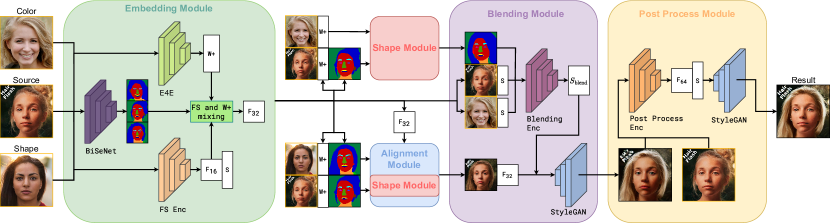
Figure 2: Overview of HairFast: first, the images go through an Embedding module where we obtain various latent representations and segmentation masks. Next, we transfer the desired hairstyle shape using Alignment module and the desired hair color using Blending module. The last step we do Post-Processing to bring back the lost details of the original image where they are needed.

In the next Alignment module we transfer the hairstyle shape from $I_{\text{shape}}$ to $I_{\text{source}}$, changing only the tensor $F$. To do this, we solve two subproblems: generating the desired hairstyle shape at the level of segmentation masks using the Shape Module, and generating $F$ tensor for inpaint after changing the shape. Once we have all the necessary $F$ tensors, we aggregate them taking into account the segmentation masks, selecting the desired parts, thus obtaining a new F tensor that corresponds to the image with the desired hair shape.

The next Blending module is designed to transfer the hair color from the $I_{\text{color}}$. To do this, we edit the $S$ space of the source image using our trained encoder, which also takes as input the $S$ tensor of the reference and additional CLIP [21] embeddings of the source images.

The image generated after the Blending module can already be considered as the final image, but in our work we also introduce a new Post-Processing module. The purpose of this module is to restore the necessary details of the original image that were lost during the Embedding module. This allows us to preserve the identity of the face and increase the realism of the method.

3.2 Embedding

The first step to edit a hairstyle is to get a projection in StyleGAN space. Methods like Barbershop and StyleYourHair explicitly run an optimization process to reconstruct each image in $FS$ space. We will in turn use a pre-trained FS encoder [35] designed specifically to immediately output $FS$ representations of input images, it is one of the highest quality encoders currently available with great image reconstruction.

The problem with $FS$ space is that it has poor editability. The native integration of the FS encoder into Barbershop results in an optimization task for color transfer that simply cannot edit $S$ space in a way that transfers hair color. To solve this problem, we additionally use E4E [29] – it is a very simple encoder with relatively poor image reconstruction quality, but has high editability. For this, we also reconstruct all images with E4E and mix the $F$ tensor corresponding to the hair with the $F$ tensor obtained with the FS encoder.

Formally, if $I$ is input image, then $F_{16}^{\text{FSE}},\ S=\text{FS}_{\text{Enc}}(I),\ w^{\text{E4E}}=\text{E4E}(I)$, where $F_{16}^{\text{FSE}}\in\mathbb{R}^{16\times 16\times 512},S\in\mathbb{R}^{12\times 512}$ – the $FS$ representation obtained from FS encoder and $w^{\text{E4E}}\in\mathbb{R}^{18\times 512}$ – the encoding from E4E.

Since we want to edit images in $F$ space of 32x32 resolution while FS encoder produces only 16x16, we need to run a few more StyleGAN blocks, while for E4E we run all 6 first blocks:

$$F_{32}^{\text{FSE}}=G_{4:6}(F_{16}^{\text{FSE}},S),\quad\quad F_{32}^{\text{E4E}}=G_{6}(w^{\text{E4E}}),$$ (1)

where $G_{6}$ – the output of the first 6 StyleGAN blocks and $G_{4:6}$ – the generator starts at block 4.

To find the hair region in the $F$ tensor, we use BiSeNet  [37] to segment a face and obtain a hair mask from it:

$$M=\text{BiSeNet}(I), H=\text{Downsample}_{32}(M=\text{hair}).$$ (2)

Then final reconstruction for images:

$$F_{32}^{\text{mix}}=\overline{H}\cdot F_{32}^{\text{FSE}}+(1-\alpha)\cdot H\cdot F_{32}^{\text{FSE}}+\alpha\cdot H\cdot F_{32}^{\text{E4E}}.$$ (3)

Here $\overline{H}$ is an inversion of the mask $H$ and $\alpha$ is the hyperparameter for mixing. In our work it is equal to 0.95. This means that we only take 5% of the hair from FS encoder, but according to our experiments, even this small mixing with the hair $F$ tensor of FS encoder hair greatly increases the quality. The visualization of the mixing procedure shown in Fig. 3.

This $F_{32}^{\text{mix}}$ tensor allows us to get an excellent quality of face and background reconstruction and still edit the hairstyle.

The output of this module are segmentation and hair masks: $M$, $H$, and embeddings $w^{\text{E4E}}$, $S$, and $F_{32}^{\text{mix}}$ for each image $I_{\text{source}}$, $I_{\text{shape}}$, and $I_{\text{color}}$.

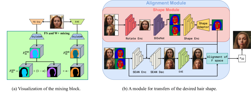
Figure 3: Detailed diagram of the units. (a) Mixing block from Embedding module mixes FS and W+ space representations to allow color editing (b) An alignment module diagram that takes the images themselves, their segmentation masks, $W+$ and $F$ representations to transfer the desired hairstyle shape.

3.3 Alignment

In this step, our goal is to transfer the desired hair shape from $I_{\text{shape}}$ to $I_{\text{source}}$. For this purpose, we edit only the $F$ space. To achieve this, we solve 2 subtasks: generation of a target mask with the desired hair shape and generation of $F$ tensor with the inpainted parts of the image.

The task of generating a target mask without optimization problems was very successfully solved by the authors of the CtrlHair [7] method using Shape Encoder, which encodes the segmentation masks of two images as separate embeddings of hair and face, and Shape Adaptor reconstructs the segmentation mask of the desired face with the desired hair shape, additionally performing inpaint. According to our experiments, this combination of Shape Encoder and Shape Adaptor performs better than the original Barbershop optimization problem, but nevertheless, this approach still has problems.

First of all, the Shape Adaptor and Shape Encoder itself has been trained to transfer the hair shape as it is in the current pose and so for the case where the source and shape photos have too different poses, the method performs very poorly, causing the final photo to show severe hair shifts. The authors of CtrlHair have partially solved this problem with a slow and ineffective post-processing of the mask.

To fix this problem, we train an additional Rotate Encoder that is trained to rotate the shape image to the same pose as the source image. This is accomplished by changing the $w^{\text{E4E}}$ representation, after which the new image is segmented and given to the input of the Shape Encoder and Shape Adaptor as the desired hair shape. Since we don’t need detailed hair to generate the mask, we use the E4E representation of the image. The Encoder itself has been trained with very good interpolation and can rotate the image to the most complex pose while maintaining the original shape of the hair. At the same time, Encoder does not mess up the hairstyles if the image poses already match.

$$w_{\text{rotate}}=\text{Rotate}_{\text{Enc}}(w_{\text{source}}^{\text{E4E}},\ w_{\text{shape}}^{\text{E4E}}), M_{\text{rotate}}=\text{BiSeNet}(G(w_{\text{rotate}})).$$ (4)

For training Rotate Encoder, we used keypoint optimization with a pre-trained STAR [38] model as well as cycle-consistency reconstruction loss. See the Appendix 8.1 for more information about the Rotate Encoder.

This approach allows for a high quality transfer of most hairstyles even with the most complex pose differences, correcting artifacts that occur even in the StyleYourHair method, as will be shown in the experiments section. A diagram of the Shape Module architecture is shown in Fig. 3. More formally, the generation of the final $M_{\text{align}}=\text{Shape}_{\text{Adaptor}}(\text{hair}_{\text{emb}},\ \text{face}_{\text{emb}})$, where

$$\text{hair}_{\text{emb}}=\text{Shape}^{\text{hair}}_{\text{Enc}}(M_{\text{rotate}}), \text{face}_{\text{emb}}=\text{Shape}^{\text{face}}_{\text{Enc}}(M_{\text{source}}),$$ (5)

According to the Eq. 2, we get $H_{\text{align}}$ from $M_{\text{align}}$.

These masks $H_{\text{align}}$ and $M_{\text{align}}$ from the Shape Module will be needed for the next alignment tasks – inpaint generation and shape transfer.

For the inpaint task, we use the pre-trained SEAN model, which produces style vectors for each segmentation class using the input image and its segmentation mask, and its decoder reconstructs the image using the style vectors and any new segmentation mask. Thus, using this model, we can obtain a 256x256 resolution image with the desired hair shape for both source and shape photos.

$$\text{style}_{\text{codes}}=\text{SEAN}_{\text{Enc}}(I,\ M), I^{\text{inpaint}}=\text{SEAN}_{\text{Dec}}(\text{style}_{\text{codes}},\ M_{\text{align}}).$$ (6)

To get the $F$ tensor representation of these images we use E4E. According to our experiments, the SEAN model in some cases produces strong artifacts in weakly represented segmentation classes such as ears, and due to artifacts on the target segmentation mask, it can also produce images with similar artifacts, such as when the hair is not connected to the head. E4E due to its good generalization is a good regularizer that automatically handles all such kind of artifact.

$$F_{32}^{\text{inpaint}}=G_{6}(\text{E4E}(I^{\text{inpaint}})).$$ (7)

In the current step we have two initial $F_{32}^{\text{mix}}$ tensors of images and two $F_{32}^{\text{inpaint}}$ tensors after the inpaint part. The last step Alignment of F space combines all four F tensors into one new $F_{32}^{\text{align}}$, which can be used to generate an image with a given hairstyle. To do this, we assemble the tensor by selecting its corresponding parts using segmentation masks. A diagram of the Alignment module is shown in Fig. 3.

$$F_{32}^{\text{align}} =H_{\text{align}}\cdot H_{\text{shape}}\cdot F^{\text{mix}}_{\text{shape}}+H_{\text{align}}\cdot\overline{H_{\text{shape}}}\cdot F_{\text{shape}}^{\text{inpaint}}+$$ (8)

$$+\overline{H_{\text{align}}}\cdot\overline{H_{\text{source}}}\cdot F^{\text{mix}}_{\text{source}}+\overline{H_{\text{align}}}\cdot H_{\text{source}}\cdot F_{\text{source}}^{\text{inpaint}}.$$

Here, $H_{\text{shape}}$ and $H_{\text{source}}$ are obtained from $I_{\text{shape}}$ and $I_{\text{source}}$ from Embedding module according to Eq. 2.

3.4 Blending

In the next step, we solve the problem of changing the $S$ space so as to change the hair color to the desired color. Barbershop’s previous approach was to find by optimization a convex combination of source and color $S$ vectors to generate the desired image, which is too strong constraint for this problem, causing the images to be edited insufficiently. Moreover, Barbershop used very outdated loss functions for optimization, which also caused additional artifacts to appear in the edited images.

To fix this, we adopt a similar encoder architecture called HairCLIP [31], whose goal is to predict the change in style of the source vector from two input $S$ vectors. This architecture consists of 1D modulation layers similar to those used in StyleGAN. Such layers are excellent for style changing and have good stability. Furthermore, we additionally feed the model with CLIP embeddings of the source image without hair $\text{emb}_{\text{face}}=\text{CLIP}_{\text{enc}}(I_{\text{source}}\cdot\overline{H_{\text{align}}}\cdot\overline{H_{\text{source}}})$ and CLIP embeddings of the hair only from the color image $\text{emb}_{\text{hair}}=\text{CLIP}_{\text{enc}}(I_{\text{color}}\cdot H_{\text{color}})$, where $H_{\text{align}}$ hair mask obtained from a Shape Module run to transfer a hair shape from $I_{\text{color}}$ to $I_{\text{source}}$. This helps to convey additional information about the original images that might have been lost in the embedding module, according to our experiments it also improved the result significantly. And $I_{\text{blend}}$ is the final image before post-processing:

$$S_{\text{blend}}=\text{Blend}_{\text{Enc}}(S_{\text{source}},\ S_{\text{color}},\ \text{emb}_{\text{face}},\ \text{emb}_{\text{hair}}),$$ (9)

$$I_{\text{blend}}=\text{StyleGAN}(F_{32}^{\text{align}},\ S_{\text{blend}}),$$ (10)

A diagram of the method is shown in Fig. 4.

$$\mathcal{L}_{\text{clip}}(I_{\text{1}},I_{\text{2}},M_{\text{1}},M_{\text{2}})=1-\mathrm{CosSim}_{\mathrm{CLIP}}(I_{\text{1}}\cdot M_{\text{1}},I_{\text{2}}\cdot M_{\text{2}}),$$ (11)

To train the model, we use the $\mathcal{L}_{\text{clip}}$ one of which optimizes the cosine distance between the CLIP embeddings of the final and source images on both the reconstruction and transfer of the desired color. See the Appendix 8.2 for training and encoder details.

3.5 Post-Process

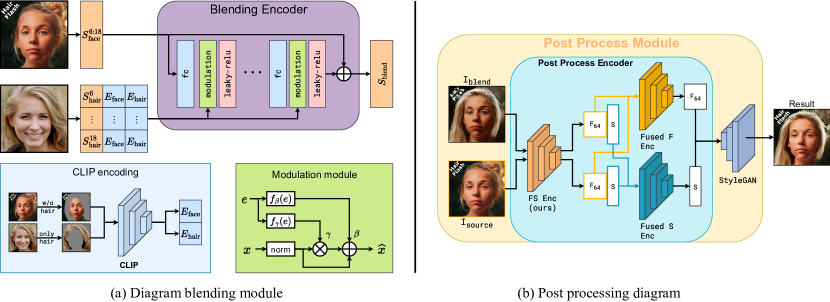
Figure 4: Detailed diagram of the units. (a) A blending module diagram that takes as input $S$ image representations as well as segmentation masks. The purpose of this block is to encode the details of the original image and change the $S$ space to transfer the desired hair color and preserve the identity. (b) A post-processing diagram that takes as input the source image and post Blending Module image. At this module, the goal is to get a new representation in StyleGAN space to get a realistic image, with the original details of the source image that were lost in the embedding module.

Experiments with baseline models showed that the FID of the CtrlHair method is the best among all other methods, although on visual comparison the method performed significantly worse than other sota approaches. Although we were able to correct this problem with a better metric, which will be discussed in the next section, the FID still considers CtrlHair to be the best performing method because of its post-processing. Their method uses Poisson blending of the original image with the final resulting image. This approach was strongly encouraged by FID metrics, but nevertheless, visually, in many cases, this blending of images is visible to the naked eye.

In turn, our method, even though it has a higher quality Blending step, still has a problem on complex cases where the face hue may change. Particularly because of this we cannot simply use Poisson blending, as the difference in shades emphasizes the overlay more and is heavily penalized by higher quality metrics.

For this reason, we are developing our own Post-Processing module, which is essentially a larger and more powerful reconstruction encoder, but for a more complex task – reconstruction of the original face and background, reconstruction of hair after Blending Module and inpaint of non-matching parts. This Post-Process encoder generates an F tensor 4 times higher resolution than the FS encoder we used in the Embedding Module. This allows for unrivaled reconstruction quality. Unlike traditional encoders that sacrifice reconstruction quality for good editing, we are able to use such a large resolution F tensor due to the fact that we do not have to edit the image after this module.

Post-Processing itself consists of a trained FS encoder at resolution 64 for the usual reconstruction task, we use it to encode the original image $I_{\text{source}}$ and the $I_{\text{blend}}$ image after our method:

$$F_{64}^{\text{blend}},\ S^{\text{blend}} =FS_{\text{Enc (ours)}}(I_{\text{blend}}),$$ (12)

$$F_{64}^{\text{source}},\ S^{\text{source}} =FS_{\text{Enc (ours)}}(I_{\text{source}}).$$ (13)

The resulting tensors F are fused using IResNet blocks. In turn, S space is fused using two similar Blending models, but without additional CLIP features. The output of this composite encoder is a 64x64 $F_{\text{final}}=\text{Fused}_{\text{F Enc}}(F_{64}^{\text{blend}},\ F_{64}^{\text{source}})$ tensor and an $S_{\text{final}}=\text{latent}_{\text{avg}}+\text{Fused}_{\text{S Enc}}(S^{\text{blend}},\ S^{\text{source}})$ vector, which are input to StyleGAN to generate the final image $I_{\text{final}}$:

$$I_{\text{final}}=\text{StyleGAN}(F_{64}^{\text{final}},\ S_{\text{final}}).$$ (14)

For model training, we use loss functions for hair reconstruction and original parts of the image, and for inpaint we use guidelines from the more robust StyleGAN space and adversarial loss. For reconstruction, these include multi-scale perceptual loss [35], DSC++ [36], ArcFace and regularizations. See the Appendix 8.3 for training and encoders details.

A diagram of the post-processing procedure is shown in the Fig. 4. This produces the final HairFast model, which is shown in the Fig. 2.

4 Experiments

Table 1: All metrics were measured on the same pre-selected triples of images (face, shape and color) from the CelebaHQ [12] dataset. Then, applying the method, FID was measured on the original dataset and the modified dataset. $\text{FID}_{\text{CLIP}}$ [17] was counted similarly to FID using the torchmetrics library, but a CLIP encoder was used instead of Inception V3. Running time was measured as the median time among a bunch of method runs, without taking into account models initialization and loading/saving images to disk.

Model	FID↓				$\text{FID}_{\text{CLIP}}$↓				Time (s)↓
	full	both	color	shape	full	both	color	shape	A100	V100
HairCLIP [31]	34.95	40.68	40.08	42.92	12.20	13.32	10.94	13.44	$0.28$	$0.36$
HairCLIPv2 [32]	$\underline{14.28}$	$\underline{23.37}$	20.21	$\underline{23.90}$	10.98	12.14	6.55	10.06	112	221
CtrlHair [7]	$15.10$	24.81	$19.65$	25.60	9.52	10.42	$\underline{3.62}$	9.59	6.57	7.87
StyleYourHair [16]	-	25.90	-	-	-	10.91	-	-	84	239
Barbershop [40]	15.94	24.52	20.54	24.08	$\underline{7.07}$	$\underline{8.12}$	3.89	$\underline{6.76}$	213	645
HairFast (ours)	$13.12$	$22.71$	$\underline{20.17}$	$23.36$	$5.12$	$6.06$	$3.00$	$5.34$	$\underline{0.41}$	$\underline{0.78}$

Realism after editing. The task of hairstyle transfer is very challenging, largely due to the lack of objective metrics. One possible metric to reflect the quality of hairstyle transfer is to measure the realism of the image using FID. To measure this metric, we consider 4 main cases: transferring hairstyle and color from different images (full), transferring only a new hairstyle shape (shape), transferring only a new color (color), and transferring both color and shape from the same image (both). To measure the metrics, we use the CelebA-HQ [12] dataset, from which we capture 1000 to 3000 experiments for each case, on which we run all methods. We used methods such as HairCLIP [31], HairCLIPv2 [32], CtrlHair [7], StyleYourHair [16] and Barbershop [40] for comparison, and for their inference we used the official code implementation. Additionally, we measure the median running time among all runs of these experiments, excluding the time to save the results to disk and initialize the neural networks.

In these experiments, we do not compare with HairNet [41], HairNeRF [3] and StyleGANSalon [15] due to the lack of their code and the inability to run the methods on our images. Instead, we compare with StyleGANSalon on images they published from their inference along with LOHO [24] in Appendix 10, and we also make a visual comparison with HairNet and HairNeRF on images from their article in Appendix 11.

For a more correct comparison, we replaced about  2% of Barbershop images that failed to generate due to an incorrect loss function that arised in the blending step when there was no hair according to BiSeNet. Instead, we used random working Barbershop images, and did so in order to preserve the sample size, which affects FID orders of magnitude.

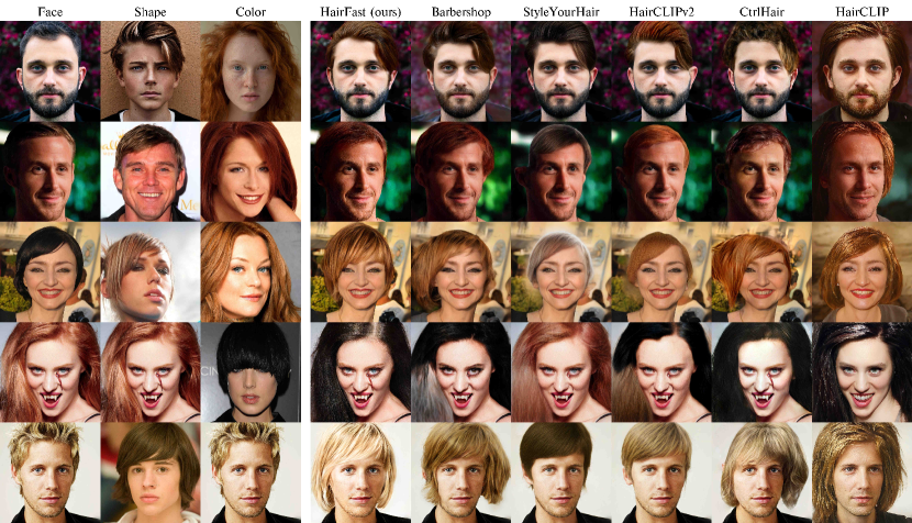
Figure 5: Visual comparison of methods on different cases for transferring hair and color together, or separately. StyleYourHair transfers color only from the Shape image. According to the results of visual comparison, our model better preserves the identity of the source image. At the same time, our method on most cases better transfers the desired hair color and texture, and works better with complex pose differences. For a more detailed comparison, see Appendix 13.

As we can see in the Tab. 1 table, a method like CtrlHair outperforms optimization-based methods like Barbershop and StyleYourHair by FID metrics. However, visual analysis reveals that the method performs much worse and artifacts are visible, which appear as a consequence of strong Poisson Blending of the final image with the original image. The authors in [17] studied the problem that makes images with strong artifacts appear more realistic by FID metric. They were able to solve this problem by using the $\text{FID}_{\text{CLIP}}$ metric, which simply uses higher quality embeddings from the CLIP model. We also compute this metric in our experiments. Note that the metric uses the CLIP-ViT-B-32 checkpoint while we use CLIP-VIT-B-16 for blending training, so there is no leakage in our measurements.

Analyzing the results, our method performs better on all cases according to the $\text{FID}_{\text{CLIP}}$ metric. But we lose to CtrlHair when transferring only hair color by FID metric because in this case CtrlHair blends almost the whole image except hair, which is strongly encouraged by the metric. Looking at runtime, we outperform Barbershop on V100 by a factor of 800 and even CtrlHair by more than 10 times. This is because CtrlHair has an expensive post-processing implementation for alignment and Poisson blending. The only method that is faster is HairCLIP, but its performance in our problem setup is quite poor.

Table 2: Pose Metrics. For this metrics, we consider color and shape transfer from the target image to the source image. For all pairs of images we calculate MAE of key facial points and split the pairs into three equal folds, which correspond to weak, medium and high pose-difference on which the corresponding metrics were measured. There were 1000 image pairs taken from CelebA-HQ. Reconstruction Metrics. For this each method is started on the task of transferring the color and shape of the hairstyle from itself to itself, thus at the end we measure the metrics with the original image. There were 3000 images taken from CelebA-HQ.

Model	Pose metrics				Reconstruction metrics
	FID↓		$\text{FID}_{\text{CLIP}}$↓
	medium	hard	medium	hard	LPIPS↓	PSNR↑	FID↓	$\text{FID}_{\text{CLIP}}$↓
HairCLIP [31]	55.77	54.35	15.53	15.73	0.36	14.08	35.49	10.48
HairCLIPv2 [32]	44.62	$\underline{45.28}$	14.56	18.66	0.16	19.71	10.09	4.08
CtrlHair [7]	46.45	50.12	12.96	16.42	0.15	19.96	$8.03$	$\underline{1.25}$
StyleYourHair [16]	46.32	47.19	13.70	15.93	0.14	$\underline{21.74}$	10.69	2.73
Barbershop [40]	$\underline{44.08}$	46.13	$\underline{11.27}$	$\underline{13.30}$	$\underline{0.11}$	21.18	13.73	2.61
HairFast (ours)	$43.25$	$44.85$	$8.90$	$10.33$	$0.08$	$23.45$	$\underline{9.72}$	$0.97$

Pose difference. Table Tab. 2 shows the results of the metrics on a subsample of our main experiment (both), but split into different cases of pose difference. For this purpose, we counted the RMSE of key points of the source image with the shape image and split all cases of hairstyle transfer into 3 equal folds: easy, medium and hard. The last two cases are presented in the table.

Reconstruction. Another quality metric can be the reconstruction metric, where each method tries to transfer the shape and color of the hairstyle from itself, in this case we have a ground truth image with which we can measure the metrics. Besides FID and $\text{FID}_{\text{CLIP}}$, which we measure with the original images and not the whole dataset, we consider the metrics LPIPS and PSNR. 3000 random images from CelebA-HQ were taken for reconstruction.

Analyzing the results Tab. 2, we see that we lose only to CtrlHair method on FID. This confirms the effectiveness of our Post-Processing, which recovers lost image details during encoding, outperforming even optimization-based methods.

Overall comparison. The Tab. 3 shows a comparison of the characteristics of the methods. Hair realism was determined according to realism metrics on reconstruction tasks and visual comparison. HairCLIPv2 has medium realism because of poor reconstruction, which due to the peculiarities of the architecture does not allow to transfer the desired texture accurately enough, in turn, CtrlHair despite the excellent metrics in visual comparison shows not similar to the desired results due to the limitations of the generator. The other methods, except HairCLIP, transfer the hairstyle realistically.

Table 3: A comparison of the characteristics of the main hair transfer methods.

	Barbershop  [40]	StyleYourHair  [16]	HairNet  [41]	HairNeRF  [3]	StyleSalon  [15]	CtrlHair  [7]	HairCLIP  [31]	HairCLIPv2  [32]	Ours
Quality
Hair realism	High	High	High	High	High	Medium	Low	Medium	High
Face-background preservation	Medium	Medium	Medium	High	High	High	Low	Medium	High
Functionality
Pose alignment	✗	✓	✓	✓	✓	✗	✗	✓	✓
Separate shape/ color transfer	✓	✗	✗	✗	✗	✓	✓	✓	✓
Efficiency
W/o optimization	✗	✗	✗	✗	✗	✓	✓	✗	✓
Runtime	>10m	>3m	>3m	>3m	>10m	>5s	<1s	>3m	<1s
Reproducibility
Code access	✓	✓	✗	✗	✗	✓	✓	✓	✓

When it comes to preserving face and background details, the latent space of methods in which image inversions take place is mainly responsible for this. Methods such as Barbershop, StyleYourHair, HairNet and HairCLIPv2 use FS resolution space 32, which does not allow them to preserve much details. In turn, the HairNeRF and StyleGANSalon methods use PTI, which allows them to preserve more details of the original image, and the CtrlHair method uses Poisson Blending, which also allows direct transfer of all original details. Our method uses FS resolution space 64, which when compared visually and reconstruction metrics shows even better quality than methods with PTI. HairCLIP, in contrast, uses the weakest W+ space.

The runtime of each method that has a code we tested independently on the Nvidia V100. StyleGANSalon’s time estimate came from their article, where they claim to run longer than Barbershop, while methods like HairNet and HairNeRF use PTI which makes them take at least a few minutes per image.

Looking at the rest of the features, unlike some other methods we are able to transfer hair color and shape independently, we are also able to handle large pose differences and our entire architecture consists of encoders, which allows us to work very fast. Moreover our method has code for inference, all pre-trained weights and scripts for training for full reproducibility.

Ablation study. As ablation, we remove some parts of our method and replace them with Barbershop optimization processes if necessary. On these configurations we measure the realism metrics after the hairstyle transfer, the results of which can be seen in the table Tab. 4 and images Fig. 7.

Configuration	FID↓	$\text{FID}_{\text{CLIP}}$↓	Time (s)↓
A Baseline	16.23	6.92	0.67
B w/o Blending Encoder	26.88	11.45	39
C w/o F mix.	16.57	6.72	$\underline{0.67}$
D config B w/o F mix.	27.74	11.51	39
E w/o Rotate Encoder	16.87	7.52	${\bf 0.62}$
F w/o Shape Adaptor	18.72	6.37	37
G w/o SEEN inpaint	${\bf 12.79}$	${\bf 4.58}$	92
H + Post-Process (ours)	$\underline{13.12}$	$\underline{5.12}$	0.78

Table 4: Ablation results. Baseline is HairFast, but without Post-Processing. In each configuration we remove only the specified part from HairFast and replace them with optimizations from Barbershop if necessary.

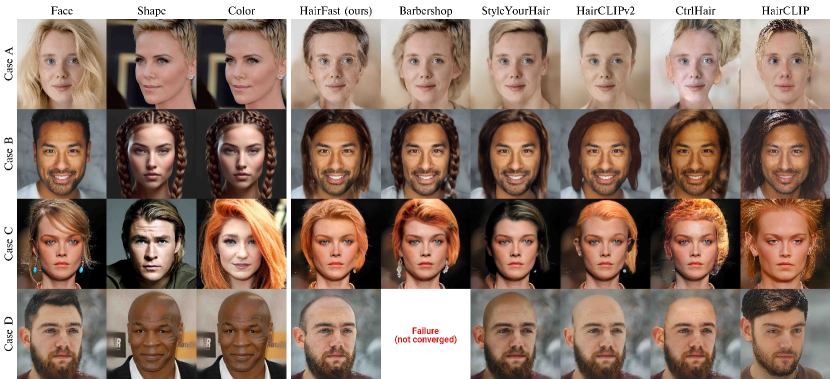
Figure 6: Failed cases. Case A poor color transfer and unrealistic inpaint. Case B unsuccessful transfer of complex texture. Case C earrings did not transfer. Case D unwanted hair in bald hairstyle transfer.

By ablation, we proved the high quality of Blending Encoder, the necessity of mixing F spaces in the embedding module, the effectiveness of Rotate Encoder, Shape Adaptor, SEEN, and the effectiveness of Post-Process module. For more detailed ablation conclusions, see Appendix 7.

Failure cases. The Fig. 6 shows examples of cases where our method does not work correctly. In particular, inpaint may not work very well for cases where long hair is replaced by short hair, in part by creating an unrealistic skin texture, or by creating shadows from past hair as in Figure 6A. In some cases, color reproduction with blending encoder does not work perfectly, in particular, the problem may occur when there is a large difference in illumination, an example of failed color reproduction is shown in Figure 6A. Also, our approach does not allow to transfer hairstyles with complex textures, such as ponytails, ribbons, braids as in the figure 6B. In addition, the model may have a problem retaining the original attributes that are exposed in the Alignment step, in which case the Post-Process may not be able to restore them (Figure 6C). Furthermore, our method may fail to remove some of the hair when transferring a bald hairstyle (Figure 6D). While these problems are important, they are inherent in all baseline models and we will address them in our future work.

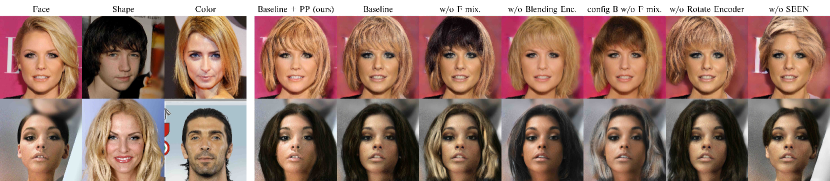
Figure 7: Ablation Study for different configurations of our model. Our model is used as the Baseline, but without Post-Processing. Each column represents a change in the Baseline of the model.

5 Conclusion and Limitations

In this article, we introduced the new HairFast method for hair transfer. Unlike other approaches, we were able to achieve high quality and high resolution comparable to other optimization-based methods, but still working in near real time. We also developed a new technique for handling photos with large pose differences, which shows better results than previous methods. We were able to achieve all this through a new architecture and quality post-processing based on encoders operating in StyleGAN’s latent space.

But our method, like many others, is limited by the small number of ways to transfer hairstyles, but our architecture allows to fix this in future work. For example, our Blending Module architecture allows similarly to HairCLIP to do hair color editing with text, and using Shape Adaptor allows similarly to CtrlHair to edit hair shape with sliders.

We prove the effectiveness of our approach by comparing it with other methods in the Sec. 4, and refer to additional experiments in the Appendix 10, 11, 12 and 13 for further details.

6 Acknowledgments

This research was supported in part through computational resources of HPC facilities at HSE University.

Appendix

In this appendix, we provide additional explanations, experiments, and results:

• Section 7: Detailed analysis of ablation results and additional metrics.

• Section 8: Model architectures, learning process and hyperparameters.

• Section 9: Additional speed measurements in different operating modes and implementation details.

• Section 10: Comparison to StyleGAN-Salon [15] and LOHO [24] on the realism metric.

• Section 11: Comparison with HairNet [41] and HairNeRF [3] visually and in terms of features.

• Section 12: Our attempts to find a color transfer metric.

• Section 13: Examples of how our method works and comparisons with others, including StyleGAN-Salon.

7 Ablation detail

7.1 Blending Encoder and F space mixing

To prove the effectiveness of our Blending Encoder and the necessity of mixing F spaces, we perform 4 experiments: configurations A – D in Tab. 4, in which we measure metrics on 1000 random triples from the CelebA-HQ dataset.

We first compare Baseline (config A) with configurations without mixing F spaces (config C), examining the results of the metrics we see that using full F space does not give a statistically significant gain in realism. But more importantly, if we examine the visual comparison Fig. 7, we see that F space without mixing does not allow us to edit the hair color with our Blending Encoder.

Similarly, we experiment with config B, in which we replace the Blending Encoder using the Barbershop optimization process, and config D, in which we additionally remove the mixing of F spaces. From the metrics results, we can see that using such an optimization process significantly degrades the realism metrics, which proves the effectiveness of our approach. Moreover, on the visual comparison we see that config B can still edit the hair and get the desired hair color, but for config D we see the same problem where even the optimization process cannot get the desired hair color, which confirms the need to use F space mixing.

7.2 Rotate Encoder

Next experiment config E, we remove the Rotate Encoder from our model, essentially leaving the generation of the targeting mask as in the CtrlHair method. In terms of metrics, removing the Rotate Encoder results in reduced realism in both FID and $\text{FID}_{\text{CLIP}}$. Moreover, when visually comparing ablations Fig. 7 we see 2 problems in this approach, which were described in detail in the Barbershop article: in case of a strong pose difference either vertically or horizontally, the hair mask adapts directly, which leads to severe distortions in the final image, but Rotate Encoder allows us to eliminate them effectively.

To verify that Rotate Encoder does not mess up the desired hair shape we additionally perform a 1000 image reconstruction experiment where we transfer the hair shape and color from the image itself to itself. For this, we compute the IOU metric on the hair mask of the original and the resulting Baseline configuration image and the config E image without Rotate Encoder. As a result, the use of Rotate Encoder led to a relative decrease in IOU by 2.7%, compared to the model without the encoder. This is a very small difference compared to the improvements seen even with small pose differences, including in Fig. 7.

7.3 Other Alignment encoders

We also run a series of experiments in which we remove one of our encoders each and replace it with a similar optimization problem from Barbershop, configuration F-G.

Analyzing the metrics of experiments E and F, we see a serious gap in all metrics, not to mention the running time due to the optimization processes.

If we consider the config G, the metrics get much better, but by visually evaluating the results in Fig. 7, we see that this optimization process strongly regularizes the desired hair shape and transfers quite differently than expected. In addition, this optimization process is very long.

This also confirms the effectiveness of our alignment step for both the task of target mask generation and inpaint not only in terms of performance but also quality.

7.4 Post Process

The last experiment config H we consider is our own HairFast model, which is Baseline (config A) with added Post-Processing. In addition to significant gains in metrics, we can also observe its effectiveness on visual comparison. Such Post-Processing effectively fixes Blending Encoder problems, for example, in cases where it cannot preserve the original face hue due to the need to change the hair color as happened in the last example Fig. 7. It also effectively reverts identity and fine details such as piercings, makeup and others.

8 Model Training

8.1 Rotate Encoder

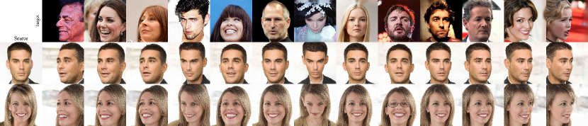
Figure 8: Demonstration of how Rotate Encoder works to rotate an image to generate the correct segmentation mask for complex pose difference images.

To train the Rotate Encoder, we collected 10’000 random images from FFHQ to learn how to rotate in W+ space from the E4E encoder to obtain an image with the desired pose. During the rotation, we must be able to preserve the shape of the hair.

The Rotate Encoder itself takes as input the first 6 vectors corresponding to the first StyleGAN blocks in W+ space of the source image and 6 vectors of the target image with the desired pose. And on the output it returns new 6 vectors, which should generate the image with the desired pose. We do not modify the remaining 18 - 6 vectors, which also helps us to preserve the identity in some details. An example of how Rotate Encoder works is shown in the image Fig. 8.

Formally, this can be described as follows:

$$w_{\text{rotate}}^{1:6}=\text{Rotate}_{\text{Enc}}(w_{\text{source}}^{\text{1:6}},w_{\text{target}}^{\text{1:6}}),$$ (15)

$$w_{\text{restore}}^{1:6}=\text{Rotate}_{\text{Enc}}(w_{\text{rotate}}^{\text{1:6}},w_{\text{source}}^{\text{1:6}}),$$ (16)

here we additionally have $w_{\text{restore}}$, which tries to turn back the modified representation. And since we do not change the last vector representations, the following is true: $w_{\text{rotate}}^{7:18}=w_{\text{restore}}^{7:18}=w_{\text{source}}^{\text{7:18}}$. And also $w_{\text{rotate}},w_{\text{restore}}\in\mathbb{R}^{18\times 512}$

During training, we randomly generate source image and target image pairs and train according to the following loss functions:

$$H_{\text{target}}=E(I_{\text{target}}),$$ (17)

$$\mathcal{L}_{\text{pose}}=||H_{\text{target}}-E(G(w_{\text{rotate}}))||_{2}^{2}.$$ (18)

In this case, $E$ – a pre-trained model for extracting 2D face key-points, we used the STAR [38] model for this purpose. For optimization, we used the first 76 key-points which corresponded to the face contour, eyebrows, eyes and nose. Thus $H_{\text{target}}\in\mathbb{R}^{76\times 2}$. In this way, due to $\mathcal{L}_{\text{pose}}$ loss, we train the model to rotate the image to the required pose for hair alignment.

The following loss functions are used to keep the original shape of the hair:

$$\mathcal{L}_{\text{recon}}=||w_{\text{source}}^{\text{E4E}}-w_{\text{restore}}||_{2}^{2},$$ (19)

$$\mathcal{L}_{\text{id}}=\text{ArcFace}(I_{\text{source}},G(w_{\text{rotate}})).$$ (20)

Here the main loss function for attribute conservation is $\mathcal{L}_{\text{recon}}$, it is what motivates the model to learn transformations that do not change the attributes of the image other than its pose. In this case, when we have rotated the image and requires to rotate it to the original pose, we know the ground truth and in this loss function we just take L2 between it. The loss function $\mathcal{L}_{\text{id}}$ is only a guide and also helps to preserve attributes a bit when rotating.

Total final loss function:

$$\mathcal{L}=\frac{\lambda_{\text{pose}}\cdot\mathcal{L}_{\text{pose}}}{\text{EMA}_{t}(\mathcal{L}_{\text{pose}})}+\frac{\lambda_{\text{recon}}\cdot\mathcal{L}_{\text{recon}}}{\text{EMA}_{t}(\mathcal{L}_{\text{recon}})}+\frac{\lambda_{\text{id}}\cdot\mathcal{L}_{\text{id}}}{\text{EMA}_{t}(\mathcal{L}_{\text{id}})}$$ (21)

The main challenge in training this model is to find the correct coefficients for the given loss functions. The model learns to adopt the correct pose very quickly and because of this, ArcFace soon begins to dominate, and with heavy overtraining, artifacts begin to form because of it. To avoid this, we first normalize the loss functions by their exponential moving average (EMA), which we compute with a factor of $t=0.02$. This allows us to maintain the correct prioritization of the loss functions throughout training.

The final model was trained with $\lambda_{\text{pose}}=6,\lambda_{\text{recon}}=2,\lambda_{\text{id}}=1$. The optimizer was Adam with learning rate $1\times 10^{-4}$ and weight decay $1\times 10^{-6}$. Batch size 16.

The architecture of the model is similar to the one used in Blending Encoder Fig. 4. We predict the change of $w_{\text{source}}^{\text{1:6}}\in\mathbb{R}^{6\times 512}$, and input $w_{\text{target}}^{\text{1:6}}\in\mathbb{R}^{6\times 512}$ to the modulation layer. In total, there are 5 blocks in the model form $\mathrm{Linear}(512,512)\to\mathrm{Modulation}\to\mathrm{LeakyReLU}(0.01)$. The block diagram of the Modulation block can be seen on the Fig. 4. The $f_{\beta}$ and $g_{\gamma}$ are $\mathrm{Linear}(512,512)\to\mathrm{LayerNorm}(512)\to\mathrm{LeakyReLU}(0.01)\to\mathrm{Linear}(512,512)$.

8.2 Blending Encoder

To train the Blending Encoder, we collect about 5800 image pairs from the FFHQ dataset. For this purpose, we run our model on 3000 triples from FFHQ and save FS spaces of source, shape and color images after Embedding Module, and then run Alignment Module to transfer hair shape from shape image to source image and additionally run one more time to transfer hair shape from color image to source. The resulting F spaces are also saved. This allows us to create 6000 pairs for color transfer, which we additionally filter and discard images without hair, from which we can not take the desired color.

Thus each object in the training sample consists of $I_{\text{source}}$, $S_{\text{source}}$ and $F_{\text{source}}^{\text{align}}$ of the original image with the hair shape from the color image, and $I_{\text{color}}$, $S_{\text{color}}$ of the color image. Our goal is to modify $S_{\text{source}}$ to get the same hair color as $I_{\text{color}}$ with the given $F_{\text{source}}^{\text{align}}$ tensor.

The first thing we do for model training is to prepare the masks:

$$H_{\text{color}}=(\text{BiSeNet}(I_{\text{color}})=\text{hair}),$$ (22)

$$H_{\text{source}}=(\text{BiSeNet}(I_{\text{source}})=\text{hair}),$$ (23)

$$H_{\text{align}}=(\text{BiSeNet}(\text{G}(F_{\text{source}}^{\text{align}},S_{\text{source}}))=\text{hair}),$$ (24)

$$M_{\text{target}}=\overline{H_{\text{source}}}\cdot\overline{H_{\text{align}}}.$$ (25)

Now we can apply our model:

$$\text{emb}_{\text{face}}=\text{CLIP}_{\text{enc}}(I_{\text{source}}\cdot M_{\text{target}}),$$ (26)

$$\text{emb}_{\text{hair}}=\text{CLIP}_{\text{enc}}(I_{\text{color}}\cdot H_{\text{color}}),$$ (27)

$$S_{\text{blend}}=\text{Blend}_{\text{Enc}}(S_{\text{source}},\ S_{\text{color}},\ \text{emb}_{\text{face}},\ \text{emb}_{\text{hair}}),$$ (28)

$$I_{\text{blend}}=\text{StyleGAN}(F_{\text{source}}^{\text{align}},\ S_{\text{blend}}),$$ (29)

And now we can apply the following loss function, which worked better than LPIPS or other combinations:

$$\mathcal{L}_{\text{clip}}(I_{\text{1}},I_{\text{2}},M_{\text{1}},M_{\text{2}})=1-\mathrm{CosSim}_{\mathrm{CLIP}}(I_{\text{1}}\cdot M_{\text{1}},I_{\text{2}}\cdot M_{\text{2}}),$$ (30)

here $\mathrm{CosSim}_{\mathrm{CLIP}}$ is the cosine distance between the embedding images from the CLIP model. The images are before that multiplied by the corresponding masks M.

We get the following loss function from here, which we optimize during training for our model.

$$\mathcal{L}_{\text{color}} =\mathcal{L}_{\text{clip}}(I_{\text{blend}},I_{\text{color}},H_{\text{align}},H_{\text{color}}),$$ (31)

$$\mathcal{L}_{\text{face}} =\mathcal{L}_{\text{clip}}(I_{\text{blend}},I_{\text{source}},M_{\text{target}},M_{\text{target}}),$$ (32)

$$\mathcal{L} =\lambda_{\text{color}}\cdot\mathcal{L}_{\text{color}}+\lambda_{\text{face}}\cdot\mathcal{L}_{\text{face}}.$$ (33)

The final model was trained with $\lambda_{\text{color}}=1$ and $\lambda_{\text{face}}=1$. The optimizer was Adam with learning rate $1\times 10^{-4}$ and weight decay $1\times 10^{-6}$. Batch size 16.

The architecture of the Blending Encoder is shown in the Fig. 4. The $f_{\beta}$ and $g_{\gamma}$ are $\mathrm{Linear}(1536,1024)\to\mathrm{LayerNorm}(1024)\to\mathrm{LeakyReLU}(0.01)\to\mathrm{Linear}(1024,512)$, for a total of 5 blocks in the model.

8.3 Post Processing

To train Post-Processing, we collect 10’000 triples from FFHQ on which we run our method without Post-Processing. The image $I_{\text{blend}}$ after Blending Encoder and the original face image $I_{\text{source}}$ are the object of the training sample.

The training of this stage consisted of three parts: FS encoder training, fusers training, and the whole model finetuning.

8.3.1 Feature Style Encoder

For FS encoder training, we first obtain a reconstruction of the real image:

$$F_{64}^{\text{source}},\ S^{\text{source}}=FS_{\text{Enc (ours)}}(I_{\text{source}}),$$ (34)

$$F_{\text{style}}^{\text{source}}=\text{G}_{8}(S^{\text{source}}),$$ (35)

$$F_{64}^{\text{recon}}=\alpha\cdot F_{64}^{\text{source}}+(1-\alpha)\cdot F_{\text{style}}^{\text{source}},$$ (36)

$$I_{\text{style}}=\text{StyleGAN}(F_{\text{style}}^{\text{source}},\ S^{\text{source}}),$$ (37)

$$I_{\text{recon}}=\text{StyleGAN}(F_{64}^{\text{recon}},\ S^{\text{source}}).$$ (38)

Besides the reconstruction image from FS space here we also get the F tensor from S space and the image generated by S. Also here $\alpha$ is a parameter which is 0 at the beginning and gradually increases to 1 during the learning process. And after that we use the following loss functions:

$$\mathcal{L}_{\text{id}}(I_{\text{1}},I_{\text{2}})=\text{ArcFace}(I_{\text{1}},I_{\text{2}}),$$ (39)

$$\mathcal{L}_{\text{m\_LPIPS}}(I_{\text{1}},I_{\text{2}})=\text{m\_LPIPS}(I_{\text{1}},I_{\text{2}}),$$ (40)

$$\mathcal{L}_{\text{recon. feat}}(F_{\text{1}},F_{\text{2}})=||F_{\text{1}}-F_{\text{2}}||_{2}^{2},$$ (41)

here $\mathcal{L}_{\text{m\_LPIPS}}$ is a multi-scale perceptual loss [35] presented by the authors of FS encoder, which in addition with $\mathcal{L}_{\text{id}}$ reconstructs the original image. In turn, it will $\mathcal{L}_{\text{recon. feat}}$ help in the initial stages to obtain an F tensor similar to the F tensor created from S space, so here we throw gradients only through one F tensor, not pull them together.

Thus the final loss function for training our FS encoder:

$$\mathcal{L} =\lambda_{\text{id}}\cdot(\mathcal{L}_{\text{id}}(I_{\text{source}},I_{\text{style}})+\mathcal{L}_{\text{id}}(I_{\text{source}},I_{\text{recon}}))\ +$$ (42)

$$+\lambda_{\text{m\_LPIPS}}\cdot(\mathcal{L}_{\text{m\_LPIPS}}(I_{\text{source}},I_{\text{style}})\ +$$

$$+\mathcal{L}_{\text{m\_LPIPS}}(I_{\text{source}},I_{\text{recon}}))\ +$$

$$+\lambda_{\text{recon. feat}}\cdot\mathcal{L}_{\text{recon. feat}}(F_{\text{style}}^{\text{source}},F_{64}^{\text{source}})\ +$$

$$+\lambda_{\text{ADV}}\cdot\mathcal{L}_{\text{ADV}}(I_{\text{recon}}),$$

here we also use adversarial loss function, as a discriminator we take the pre-trained one from StyleGAN and train it in the process using the classical loss function and R1 regularization.

The following parameters were used for training: $\lambda_{\text{id}}=0.1,\lambda_{\text{m\_LPIPS}}=0.8,\lambda_{\text{recon. feat}}=0.01$ and $\lambda_{\text{ADV}}=0.2$. Adam was used for encoder optimization with learning rate $2\times 10^{-4}$ and weight decay 0, and for discriminator learning rate $1\times 10^{-4}$, betas=(0.9, 0.999) and weight decay 0. The model was trained with a batch size 16.

8.3.2 Fusing Encoders

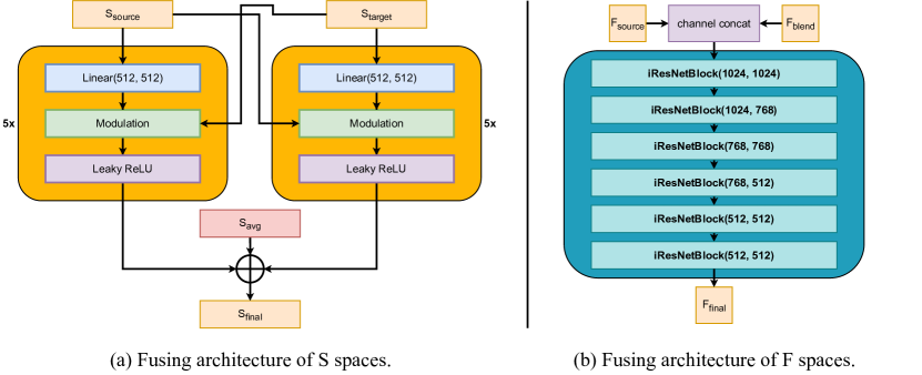
Figure 9: Diagram of fusing encoders in post processing. (a) The modulation architecture is shown in the Fig. 4. $f_{\beta}$ and $g_{\gamma}$ in modulation are $\mathrm{Linear}(512,512)\to\mathrm{LayerNorm}(512)\to\mathrm{LeakyReLU}(0.01)\to\mathrm{Linear}(512,512)$. $S_{\text{avg}}$ is the average latent vector. (b) The architecture consists of the usual IResNet blocks.

Once we have trained the FS encoder we can proceed to train models for fusing spaces. First of all we need to get FS representations from images:

$$F_{64}^{\text{blend}},\ S^{\text{blend}} =FS_{\text{Enc (ours)}}(I_{\text{blend}}),$$ (43)

$$F_{64}^{\text{source}},\ S^{\text{source}} =FS_{\text{Enc (ours)}}(I_{\text{source}}).$$ (44)

Now we can apply our models to fusing:

$$F_{\text{final}}=\text{Fused}_{\text{F Enc}}(F_{64}^{\text{blend}},\ F_{64}^{\text{source}}),$$ (45)

$$S_{\text{final}}=\text{latent}_{\text{avg}}+\text{Fused}_{\text{S Enc}}(S^{\text{blend}},\ S^{\text{source}}),$$ (46)

$$F_{\text{style}}=\text{G}_{8}(S^{\text{final}}),$$ (47)

$$I_{\text{style}}=\text{StyleGAN}(F_{\text{style}},\ S_{\text{final}}),$$ (48)

$$I_{\text{final}}=\text{StyleGAN}(F_{64}^{\text{final}},\ S_{\text{final}}).$$ (49)

Similar loss functions are used to train the encoders, but in addition we use DSC++ [36] to make the segmentation mask match the original one. We also add a loss function for inpaint. First of all, we will need new masks:

$$H_{\text{source}}=(\text{BiSeNet}(I_{\text{source}})=\text{hair}),$$ (50)

$$H_{\text{blend}}=(\text{BiSeNet}(I_{\text{blend}})=\text{hair}),$$ (51)

$$M_{\text{target}}=\overline{H_{\text{source}}}\cdot\overline{H_{\text{blend}}},$$ (52)

$$M_{\text{inpaint}}=\overline{M_{\text{target}}}\cdot\overline{H_{\text{blend}}}.$$ (53)

The inpaint is quite sensitive to the boundaries of the mask on which it is applied, so we use a special soft dilation that runs this mask through a convolution with a kernel consisting of ones in the shape of a circle of radius 25. After that we raise the result to degree 1/4, which allows us to get more concentrated values. We also create a hard mask for the $I_{\text{style}}$ guide as we don’t want to look at the hair of this image:

$$M_{\text{smooth}}=\mathrm{Dilation}(M_{\text{inpaint}}),$$ (54)

$$M_{\text{hard}}=M_{\text{smooth}}\cdot\overline{H_{\text{blend}}}.$$ (55)

The discriminator is the main contributor to inpaint, but to help ease the load on it we guide it with $\mathcal{L}_{\text{m\_LPIPS}}$ over the inpaint area using two images: $I_{\text{blend}}$ and $I_{\text{style}}$. The first one is used to guide and preserve better details, while the second image has a more correct shading.

The final loss function is as follows:

$$\mathcal{L} =\lambda_{\text{id}}\cdot(\mathcal{L}_{\text{id}}(I_{\text{source}}\cdot M_{\text{target}},I_{\text{style}}\cdot M_{\text{target}})+\$$ (56)

$$+\mathcal{L}_{\text{id}}(I_{\text{source}}\cdot M_{\text{target}},I_{\text{final}}\cdot M_{\text{target}}))\ +$$

$$+\lambda_{\text{m\_LPIPS}}\cdot(\mathcal{L}_{\text{m\_LPIPS}}(I_{\text{source}}\cdot M_{\text{target}},I_{\text{style}}\cdot M_{\text{target}})\ +$$

$$+\mathcal{L}_{\text{m\_LPIPS}}(I_{\text{source}}\cdot M_{\text{target}},I_{\text{final}}\cdot M_{\text{target}}))\ +$$

$$+\lambda_{\text{m\_LPIPS}}\cdot(\mathcal{L}_{\text{m\_LPIPS}}(I_{\text{target}}\cdot H_{\text{blend}},I_{\text{style}}\cdot H_{\text{blend}})\ +$$

$$+\mathcal{L}_{\text{m\_LPIPS}}(I_{\text{target}}\cdot H_{\text{blend}},I_{\text{final}}\cdot H_{\text{blend}}))\ +$$

$$+\lambda_{\text{recon. feat}}\cdot\mathcal{L}_{\text{recon. feat}}(F_{\text{style}},F_{\text{final}})\ +$$

$$+\lambda_{\text{DSC++}}\cdot\mathcal{L}_{\text{DSC++}}(\text{BiSeNet}(I_{\text{blend}}),\text{BiSeNet}(I_{\text{final}}))\ +$$

$$+\lambda_{\text{inpaint}}\cdot(\mathcal{L}_{\text{m\_LPIPS}}(I_{\text{style}}\cdot M_{\text{hard}},I_{\text{final}}\cdot M_{\text{hard}})\ +$$

$$+\mathcal{L}_{\text{m\_LPIPS}}(I_{\text{blend}}\cdot M_{\text{smooth}},I_{\text{final}}\cdot M_{\text{smooth}}))\ +$$

$$+\lambda_{\text{ADV}}\cdot\mathcal{L}_{\text{ADV}}(I_{\text{final}}).$$

The following parameters were used for training: $\lambda_{\text{id}}=0.1,\lambda_{\text{m\_LPIPS}}=0.4,\lambda_{\text{recon. feat}}=0.01,\lambda_{\text{DSC++}}=0.1,\lambda_{\text{inpaint}}=0.2$ and $\lambda_{\text{ADV}}=0.2$. Adam was used for encoders optimization with learning rate $2\times 10^{-4}$ and weight decay 0, and for discriminator learning rate $3\times 10^{-4}$, betas=(0.9, 0.999) and weight decay 0. The model was trained with a batch size 16.

After we have trained the fusers, we unfreeze the FS encoder and retrain the whole model with the same parameters, but with half the learning rate.

The fusing architecture of S and F spaces is presented in Fig. 9.

9 Operating modes

Each module of the method has its own strict function, but not all modes of operation require all modules.

9.1 Transferring the desired color

Thus, for the task of changing only the hair color, we do not need to run the Alignment module, since we do not need to change the hair shape.

In this mode, our method performs in 0.52 and 0.27 seconds on V100 and A100, respectively, while HairCLIP performs in 0.31 and 0.25 seconds. This enables us to achieve nearly identical speed as the fastest hair transfer methods, but still have twice the quality according to the realism metrics.

9.2 Transfer of the desired shape

Similarly, for the task of transferring only the hair shape, we do not need to run the Shape Module for the Blending Encoder, since the hair shape of the color matches the original hair shape that can be obtained from BiSeNet in the Embedding Module. However, the Blending Module must still be run for this mode, even though we want to keep the original hair color. This is necessary due to the fact that when we transfer the hair shape, the hair color from the shape image may leak into the F space, similar to what is seen in the experiments without mixing F spaces in the ablation Fig. 7. In addition, Blending Encoder recovers lost details during the embedding stage, which also improves the quality.

In this mode, our method performs in 0.71 and 0.40 seconds on V100 and A100, respectively. While in both shape and color transfer mode, the run times were 0.78 and 0.52 seconds.

9.3 Transferring hairstyle and color from one image.

This mode as well as the previous one formally works with only 2 images, which reduces the load on the encoders and also we do not need to re-run the Shape Module for Blending Encoder.

Like the previous one, it performs in 0.71 and 0.40 seconds on V100 and A100, respectively.

10 Realism after editing by StyleGAN-salon

Table 5: The task of transferring hair color and shape from the target image to the original image. Selected 450 pairs from the FFHQ dataset by the authors of StyleGAN-Salon. Images of method results are provided by the authors of StyleGAN-Salon, we compute the images for CtrlHair and our method. The table shows the realism metrics as well as the RMSE of key points of the generated face and the original face, also as this metric is shown by the authors of StyleGAN-Salon.

Model	Based	FID↓	$\text{FID}_{\text{CLIP}}$↓	RMSE↓
CtrlHair [7]	Enc.	52.14	15.27	5.48
LOHO [24]	Opt.	50.24	15.12	8.16
HairCLIPv2 [32]	Opt.	$\underline{48.95}$	14.59	5.66
StyleYourHair [16]	Opt.	52.10	12.68	7.14
Barbershop [40]	Opt.	50.76	10.37	7.31
StyleGAN-Salon [15]	Opt.	50.32	$\underline{9.91}$	$\underline{4.65}$
HairFast (ours)	Enc.	$47.15$	$8.45$	$4.52$

The authors of the StyleGAN-Salon [15] method have not yet published their code, which makes them hard to compare, but they do provide a small dataset with an inference of many basic models, including LOHO [24], one of the first optimization-based methods, as well as their own method. The StyleGAN-Salon method itself uses optimization-based methods and also PTI, which should make it very long. In the article itself, the authors talk about 21 minutes on a single input pair, but the measurements were done on a different hardware.

Unlike our past metrics, these were measured on the FFHQ dataset on which we trained our models. The authors are measured on 450 image pairs, which together did not occur in any training from our models.

Analyzing the results Tab. 5 we see that we outperform all methods on all presented metrics, including the new metric RMSE measured between key points of the original face and the generated face. This metric confirms the effectiveness of our Alignment approach, while other methods may corrupt the shape of the original face. Also, these results confirm the effectiveness of our post-processing, which outperforms even PTI in terms of realism.

Also see a visual comparison of our model with StyleGAN-Salon in Fig. 14.

11 Comparison with HairNet and HairNeRF

The authors of HairNet [41] and HairNeRF [3] have not published their code at this time, nor do they provide any datasets on which to compare with them. So instead we compare with them based on features that can be seen partially in the Tab. 3 and also visually in the images from their paper.

11.1 Comparison with HairNet

Figure 10: Visual comparison of our method with HairNet [41].

By analyzing HairNet we can highlight some key points compared to our work: (1) HairNet uses optimization based inversion and PTI for pre-processing, which implies that it must run hundreds of times slower than our method. (2) HairNet has worse FID than Barbershop and visually worse than StyleGAN Salon. Consequently, we should expect better performance. (3) HairNet works only in low FS space, so the method retains much less details than our approach. (4) Unlike our approach, HairNet is incapable of transferring hair color independent of hair shape.

Visual analysis with images reported in HairNet paper is shown in Figure 10. HairNet compared to our method tend to be poor at preserving the details of the original image and may change the identity, also the method may be worse at transferring hair texture and color.

Summarizing the above, we can say that HairNet is inferior to ours in many characteristics.

11.2 Comparison with HairNeRF

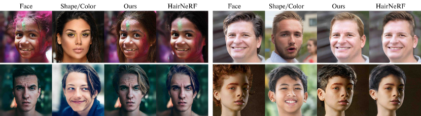
Figure 11: Visual comparison of our method with HairNeRF [3].

Unlike most other approaches HairNeRF [3] works on StyleNeRF [6] rather than StyleGAN, which makes it more difficult to compare features without their code. But in their work they use optimizations including image inversion with PTI, alignment and blending, which means they have to work hundreds of times longer than our approach. In addition, HairNeRF cannot independently transfer hair color or hair shape.

A visual comparison Fig. 11 shows the effectiveness of StyleNeRF for image alignment compared to other baseline models, but still comparable to our approach. Although HairNeRF uses PTI, our method still preserves more details of the original image and preserves the identity better.

12 Color transfer metric

In our work, we also try to find a metric for the quality of hair color transfer, other methods have not provided anything similar before. Our attempts to find a metric were aimed at using different hair loss functions or estimation models that were applied on the results when transferring random color and desired color. But no one model found a statistical difference between these results, which did not allow us to make a conclusion about the quality of the color transfer.

But we were able to get one of the estimates that showed statistical significance between random and set experiments. To do this, we convert the color image and the final image into HSV format, from which we take the pixels corresponding to the eroded hair mask for each image. After that, for each pixel coordinate corresponding to hue, saturation and value we construct a discrete distribution of values over 500 bins. Finally, we compute the similarity of the resulting discrete distributions using Jensen-Shannon divergence. The average results for 1000 random experiments from CelebA-HQ are summarized in Table Tab. 6.

Table 6: A color transfer metric that measures the Jensen-Shannon divergence between the histogram of the hue, saturation and value channel distributions of the hair of resulting image and the target hair image in HSV format. For this metric, we consider the color and shape transfer from the target image to the source image. 1000 image pairs from CelebA-HQ are taken.

Model	H mean↓	S mean↓	V mean↓
HairCLIP [31]	$0.346$	0.275	0.265
HairCLIPv2 [32]	0.418	0.291	0.278
CtrlHair [7]	$\underline{0.349}$	$0.249$	$0.236$
StyleYourHair [16]	0.429	0.310	0.290
Barbershop [40]	0.405	0.266	$\underline{0.249}$
HairFast (ours)	0.357	$\underline{0.262}$	0.269

Unfortunately, this metric doesn’t take into account too many factors, such as things like lighting in the images, but it still allows us to draw some conclusions.

So our method shows very good results for hue and saturation channels, which indicates quite accurate color reproduction. This correlates with the visual Fig. 12 and Fig. 13 comparison.

13 Visual comparison

The Fig. 12 and Fig. 13 shows the results of a visual comparison with the Barbershop [40], StyleYourHair [16], HairCLIPv2 [32], CtrlHair [7] and HairCLIP [31] methods. StyleYourHair cannot transfer the desired color from a different image, so it tried to transfer the color from the shape image. Also, for visual comparison, we disabled StyleYourHair’s horizontal flip feature, which was enabled when we calculated our metrics in the main part. This feature allows StyleYourHair to check if the reflected image will have a smaller pose difference than the original image and transfer the hairstyle from it. We disabled it in this compare to see how their approach to image rotation works compared to ours, and because most hairstyles are asymmetrical and often want to be transferred as they are in the example.

Analyzing the Fig. 12 and Fig. 13 results, in addition to the speed gain, we would like to mention the excellent quality, which in most cases outperforms other methods. For example, our method successfully captures the desired hue in all submitted images, while other methods fail. In addition, our method is much better at preserving the identity of the face, its details and its surroundings. And with all this, our method handles well the difficult cases related to pose differences, while even StyleYourHair, which is focused on this task, does worse.

We also do a visual comparison with StyleGAN-Salon in the image Fig. 14. Although their method produces PTI for each example to preserve more details of the original image, our large encoder approach performs much better and preserves much more details. This in particular allows us to better preserve the identity of the face and attributes such as glasses. This is also confirmed by the Tab. 5 metrics. In addition, StyleGAN-Salon’s 3D image rotation approach with hair shape sometimes creates artifacts on the hair, and also sometimes changes long hair to short hair because of this.

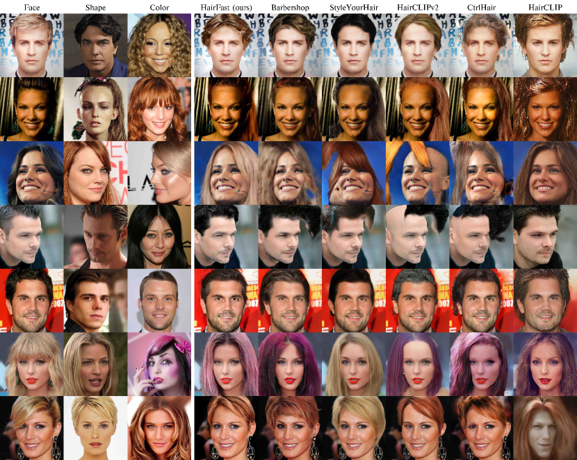
Figure 12: The first part of a visual comparison of the performance of the methods. All methods transfer hair shape and color from given images, except StyleYourHair, which due to its limitations transfers both shape and color only from Shape images.

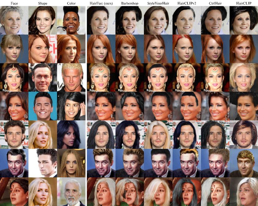
Figure 13: The second part of a visual comparison of the performance of the methods. All methods transfer hair shape and color from given images, except StyleYourHair, which due to its limitations transfers both shape and color only from Shape images.

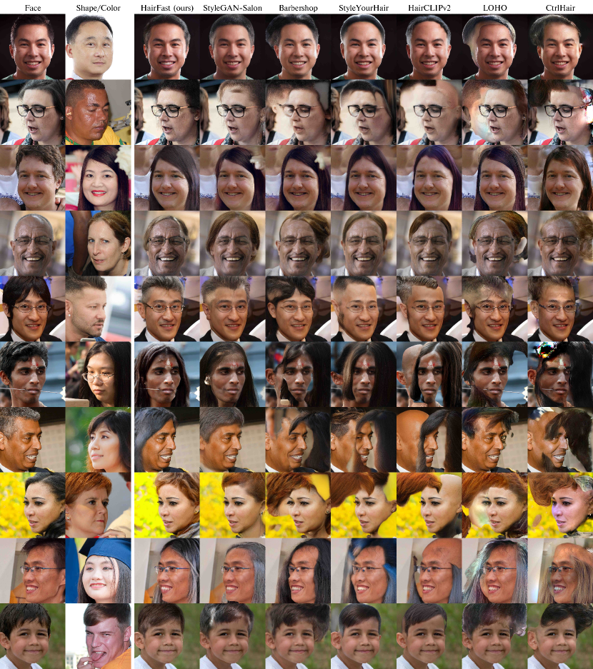
Figure 14: Visual comparison with pictures presented by the authors of StyleGAN Salon, where we are additionally compared to their model as well as LOHO.

References

- [1] Abdal, R., Qin, Y., Wonka, P.: Image2stylegan: How to embed images into the stylegan latent space? In: Proceedings of the IEEE/CVF international conference on computer vision. pp. 4432–4441 (2019)
- [2] Chan, E.R., Lin, C.Z., Chan, M.A., Nagano, K., Pan, B., De Mello, S., Gallo, O., Guibas, L.J., Tremblay, J., Khamis, S., et al.: Efficient geometry-aware 3d generative adversarial networks. In: Proceedings of the IEEE/CVF Conference on Computer Vision and Pattern Recognition. pp. 16123–16133 (2022)
- [3] Chang, S., Kim, G., Kim, H.: Hairnerf: Geometry-aware image synthesis for hairstyle transfer. In: Proceedings of the IEEE/CVF International Conference on Computer Vision. pp. 2448–2458 (2023)
- [4] Chung, C., Kim, T., Nam, H., Choi, S., Gu, G., Park, S., Choo, J.: Hairfit: pose-invariant hairstyle transfer via flow-based hair alignment and semantic-region-aware inpainting. arXiv preprint arXiv:2206.08585 (2022)
- [5] Goodfellow, I., Pouget-Abadie, J., Mirza, M., Xu, B., Warde-Farley, D., Ozair, S., Courville, A., Bengio, Y.: Generative adversarial nets. Advances in neural information processing systems 27 (2014)
- [6] Gu, J., Liu, L., Wang, P., Theobalt, C.: Stylenerf: A style-based 3d-aware generator for high-resolution image synthesis (2021)
- [7] Guo, X., Kan, M., Chen, T., Shan, S.: Gan with multivariate disentangling for controllable hair editing. In: European Conference on Computer Vision. pp. 655–670. Springer (2022)
- [8] Heusel, M., Ramsauer, H., Unterthiner, T., Nessler, B., Hochreiter, S.: Gans trained by a two time-scale update rule converge to a local nash equilibrium. Advances in neural information processing systems 30 (2017)
- [9] Isola, P., Zhu, J.Y., Zhou, T., Efros, A.A.: Image-to-image translation with conditional adversarial networks. In: Proceedings of the IEEE conference on computer vision and pattern recognition. pp. 1125–1134 (2017)
- [10] Jiang, W., Liu, S., Gao, C., Cao, J., He, R., Feng, J., Yan, S.: Psgan: Pose and expression robust spatial-aware gan for customizable makeup transfer. In: Proceedings of the IEEE/CVF Conference on Computer Vision and Pattern Recognition. pp. 5194–5202 (2020)
- [11] Jo, Y., Park, J.: Sc-fegan: Face editing generative adversarial network with user’s sketch and color. In: Proceedings of the IEEE/CVF international conference on computer vision. pp. 1745–1753 (2019)
- [12] Karras, T., Aila, T., Laine, S., Lehtinen, J.: Progressive growing of gans for improved quality, stability, and variation. arXiv preprint arXiv:1710.10196 (2017)
- [13] Karras, T., Laine, S., Aila, T.: A style-based generator architecture for generative adversarial networks. In: Proceedings of the IEEE/CVF conference on computer vision and pattern recognition. pp. 4401–4410 (2019)
- [14] Karras, T., Laine, S., Aittala, M., Hellsten, J., Lehtinen, J., Aila, T.: Analyzing and improving the image quality of stylegan. In: Proceedings of the IEEE/CVF conference on computer vision and pattern recognition. pp. 8110–8119 (2020)
- [15] Khwanmuang, S., Phongthawee, P., Sangkloy, P., Suwajanakorn, S.: Stylegan salon: Multi-view latent optimization for pose-invariant hairstyle transfer. In: Proceedings of the IEEE/CVF Conference on Computer Vision and Pattern Recognition. pp. 8609–8618 (2023)
- [16] Kim, T., Chung, C., Kim, Y., Park, S., Kim, K., Choo, J.: Style your hair: Latent optimization for pose-invariant hairstyle transfer via local-style-aware hair alignment. In: European Conference on Computer Vision. pp. 188–203. Springer (2022)
- [17] Kynkäänniemi, T., Karras, T., Aittala, M., Aila, T., Lehtinen, J.: The role of imagenet classes in fréchet inception distance. In: Proc. ICLR (2023)
- [18] Lee, C.H., Liu, Z., Wu, L., Luo, P.: Maskgan: Towards diverse and interactive facial image manipulation. In: Proceedings of the IEEE/CVF Conference on Computer Vision and Pattern Recognition. pp. 5549–5558 (2020)
- [19] Park, T., Liu, M.Y., Wang, T.C., Zhu, J.Y.: Semantic image synthesis with spatially-adaptive normalization. In: Proceedings of the IEEE/CVF conference on computer vision and pattern recognition. pp. 2337–2346 (2019)
- [20] Portenier, T., Hu, Q., Szabo, A., Bigdeli, S.A., Favaro, P., Zwicker, M.: Faceshop: Deep sketch-based face image editing. arXiv preprint arXiv:1804.08972 (2018)
- [21] Radford, A., Kim, J.W., Hallacy, C., Ramesh, A., Goh, G., Agarwal, S., Sastry, G., Askell, A., Mishkin, P., Clark, J., et al.: Learning transferable visual models from natural language supervision. In: International conference on machine learning. pp. 8748–8763. PMLR (2021)
- [22] Richardson, E., Alaluf, Y., Patashnik, O., Nitzan, Y., Azar, Y., Shapiro, S., Cohen-Or, D.: Encoding in style: a stylegan encoder for image-to-image translation. In: Proceedings of the IEEE/CVF conference on computer vision and pattern recognition. pp. 2287–2296 (2021)
- [23] Roich, D., Mokady, R., Bermano, A.H., Cohen-Or, D.: Pivotal tuning for latent-based editing of real images. ACM Transactions on graphics (TOG) 42(1), 1–13 (2022)
- [24] Saha, R., Duke, B., Shkurti, F., Taylor, G.W., Aarabi, P.: Loho: Latent optimization of hairstyles via orthogonalization. In: Proceedings of the IEEE/CVF Conference on Computer Vision and Pattern Recognition. pp. 1984–1993 (2021)
- [25] Tan, Z., Chai, M., Chen, D., Liao, J., Chu, Q., Liu, B., Hua, G., Yu, N.: Diverse semantic image synthesis via probability distribution modeling. In: Proceedings of the IEEE/CVF Conference on Computer Vision and Pattern Recognition. pp. 7962–7971 (2021)
- [26] Tan, Z., Chai, M., Chen, D., Liao, J., Chu, Q., Yuan, L., Tulyakov, S., Yu, N.: Michigan: multi-input-conditioned hair image generation for portrait editing. arXiv preprint arXiv:2010.16417 (2020)
- [27] Tan, Z., Chen, D., Chu, Q., Chai, M., Liao, J., He, M., Yuan, L., Hua, G., Yu, N.: Efficient semantic image synthesis via class-adaptive normalization. IEEE Transactions on Pattern Analysis and Machine Intelligence 44(9), 4852–4866 (2021)
- [28] Tewari, A., Elgharib, M., Bernard, F., Seidel, H.P., Pérez, P., Zollhöfer, M., Theobalt, C.: Pie: Portrait image embedding for semantic control. ACM Transactions on Graphics (TOG) 39(6), 1–14 (2020)
- [29] Tov, O., Alaluf, Y., Nitzan, Y., Patashnik, O., Cohen-Or, D.: Designing an encoder for stylegan image manipulation. ACM Transactions on Graphics (TOG) 40(4), 1–14 (2021)
- [30] Wang, T.C., Liu, M.Y., Zhu, J.Y., Tao, A., Kautz, J., Catanzaro, B.: High-resolution image synthesis and semantic manipulation with conditional gans. In: Proceedings of the IEEE conference on computer vision and pattern recognition. pp. 8798–8807 (2018)
- [31] Wei, T., Chen, D., Zhou, W., Liao, J., Tan, Z., Yuan, L., Zhang, W., Yu, N.: Hairclip: Design your hair by text and reference image. In: Proceedings of the IEEE/CVF Conference on Computer Vision and Pattern Recognition. pp. 18072–18081 (2022)
- [32] Wei, T., Chen, D., Zhou, W., Liao, J., Zhang, W., Hua, G., Yu, N.: Hairclipv2: Unifying hair editing via proxy feature blending (2023)
- [33] Xiao, C., Yu, D., Han, X., Zheng, Y., Fu, H.: Sketchhairsalon: Deep sketch-based hair image synthesis. arXiv preprint arXiv:2109.07874 (2021)
- [34] Yang, S., Wang, Z., Liu, J., Guo, Z.: Deep plastic surgery: Robust and controllable image editing with human-drawn sketches. In: Computer Vision–ECCV 2020: 16th European Conference, Glasgow, UK, August 23–28, 2020, Proceedings, Part XV 16. pp. 601–617. Springer (2020)
- [35] Yao, X., Newson, A., Gousseau, Y., Hellier, P.: A style-based gan encoder for high fidelity reconstruction of images and videos. European conference on computer vision (2022)
- [36] Yeung, M., Rundo, L., Nan, Y., Sala, E., Schönlieb, C.B., Yang, G.: Calibrating the dice loss to handle neural network overconfidence for biomedical image segmentation. Journal of Digital Imaging 36(2), 739–752 (2023)
- [37] Yu, C., Wang, J., Peng, C., Gao, C., Yu, G., Sang, N.: Bisenet: Bilateral segmentation network for real-time semantic segmentation. In: European Conference on Computer Vision. pp. 334–349. Springer (2018)
- [38] Zhou, Z., Li, H., Liu, H., Wang, N., Yu, G., Ji, R.: Star loss: Reducing semantic ambiguity in facial landmark detection. In: Proceedings of the IEEE/CVF Conference on Computer Vision and Pattern Recognition (CVPR). pp. 15475–15484 (June 2023)
- [39] Zhu, J., Shen, Y., Zhao, D., Zhou, B.: In-domain gan inversion for real image editing. In: European conference on computer vision. pp. 592–608. Springer (2020)
- [40] Zhu, P., Abdal, R., Femiani, J., Wonka, P.: Barbershop: Gan-based image compositing using segmentation masks. arXiv preprint arXiv:2106.01505 (2021)
- [41] Zhu, P., Abdal, R., Femiani, J., Wonka, P.: Hairnet: Hairstyle transfer with pose changes. In: European Conference on Computer Vision. pp. 651–667. Springer (2022)
- [42] Zhu, P., Abdal, R., Qin, Y., Femiani, J., Wonka, P.: Improved stylegan embedding: Where are the good latents? arXiv preprint arXiv:2012.09036 (2020)
- [43] Zhu, P., Abdal, R., Qin, Y., Wonka, P.: Sean: Image synthesis with semantic region-adaptive normalization. In: Proceedings of the IEEE/CVF Conference on Computer Vision and Pattern Recognition. pp. 5104–5113 (2020)