Mitigating Transient Bullwhip Effects Under Imperfect Demand Forecasts

Abstract

Motivated by how forecast errors exacerbate order fluctuations in supply chains, we use tools from robust control theory to characterize and compute the worst-case order fluctuation experienced by an individual supply chain vendor under bounded forecast errors and demand fluctuations. Building on existing discrete time, linear time-invariant (LTI) models of supply chains, we separately model forecast error and demand fluctuations as inputs to the inventory dynamics. We then define a transient Bullwhip measure to evaluate the vendor’s worst-case order fluctuation and show that for bounded forecast errors and demand fluctuations, this measure is equivalent to the disturbance to control peak gain. To compute the controller that minimizes the worst-case peak gain, we formulate an optimization problem with bilinear matrix inequalities and show that solving this problem is equivalent to minimizing a quasi-convex function on a bounded domain. In contrast to the existing Bullwhip measure in literature, the transient Bullwhip measure has an explicit dependency on the forecast error and does not need the forecast to be a deterministic function of the demand history. This explicit dependency enables us to separately quantify the transient Bullwhip measure’s sensitivity to forecast error and demand fluctuations. We empirically verify our model for vendors with non-zero perishable rates and order backlogging rates.

I Introduction

As modern supply chains become more interconnected both geographically and between different commodities, an individual disruption’s impact on the global supply chain has compounded [1]. Individual supply chain components are connected to a greater number of disruptions worldwide, such that individual disruptions have greater capacity to cause global supply chain failures [2, 3].

In supply chain management, the amplification of demand fluctuations to upstream suppliers is termed the Bullwhip effect [4]. Both behavioral and mathematical analyses of this phenomenon have pointed to demand forecast errors as the Bullwhip effect’s major instigator [5, 6]. Unfortunately, as predictors of the future, demand forecasts will unavoidably have errors. These errors induce 1) conservative ordering [7], when upstream suppliers over-react to demand forecasts by overstocking supplies; 2) virtual inflation [8], when consumers suspect potential supply shortages and overwhelm the supply chain; and 3) information withholding [9], when competing supply chain components prevent accurate demand signals from reaching their suppliers to retain greater market power in the supply chain. All three of these phenomena worsen the Bullwhip effect.

Despite their potential to instigate the Bullwhip effect, forecasts are irreplaceable in supply chain management. Due to the time it takes to fulfill orders and to physically transport goods, inventory managers must always place their orders based on the forecasted future demand. Thus, the Bullwhip effect cannot be tamed without explicitly accounting for forecast errors. On the other hand, while robust control theory specifically deals with stabilizing disturbance-prone dynamical systems, most of the existing supply chain analysis under the robust control framework assumes that the forecast is a unique function of the historical demand. Thus, many of the results do not generalize to alternative forecasting techniques and conflate the impact of forecasting errors with the impact of demand fluctuations. Presently, we address the following question: is it possible to model the forecast-driven inventory dynamics as a state-based linear system, and apply robust control techniques to mitigate its transient demand amplification?

We specifically focus on the transient demand amplification as opposed to the asymptotic total demand amplification that is used as the standard proxy for the Bullwhip effect in supply chain literature [10, 11]. Historically, most supply and demand trends stabilize in the long term, but the transient fluctuations will still lead to supply chain loss. For example, chicken wings were at first overstocked and then under-supplied at the beginning and middle of the COVID-19 pandemic, respectively [12]. While the chicken wing supply chain has restabilized, these fluctuations led to significant and irreversible food wastage.

Contributions. Building on an existing state-space, discrete-time LTI model [11] of a single commodity vendor with non-zero order backlog rates, we incorporate imperfect demand forecast both as a disturbance-driven variable and a feedforward term to augment the state-based feedback control. From this model, we define the transient Bullwhip measure as the worst-case peak gain from forecast errors and demand fluctuations to order fluctuations. We show that the bilinear matrix inequality that bounds the peak gain of a given forecast-driven feedback controller can be reduced to a linear matrix inequality. Furthermore, we show that the transient Bullwhip measure depends nonlinearly on the worst-case magnitudes of the forecasting errors and the demand fluctuations, and empirically compare the impact of different backlog and commodity perishing rates on the transient Bullwhip measure.

Although we formulate and compute the transient Bullwhip measure for a single vendor, our results can extend to the multi-vendor setting. Mitigating the Bullwhip effect in the multi-vendor setting is more challenging due to the Bullwhip effect’s dependence on the supply chain’s interaction and communication structure [13, 10].

The paper is organized as follows: in Section II, we define our forecast-driven inventory control problem and the corresponding LTI under both perfect forecast and stationary demand as well as imperfect forecast and fluctuating demand. In Section III, we define the transient Bullwhip measure using the $\ell_{\infty}$ gain, relate it to a minimization problem over bilinear matrix inequalities, and reduce it to a quasi-convex function of a single variable. In Section V-A, we apply our results to single commodity vendors with different perishing and backlogging rates to gain new insights into how to minimize the transient Bullwhip effect.

II Supply chain Inventory Model

We consider the discrete-time dynamics of a single-product supply chain vendor that orders and resupplies at fixed time intervals and is subjected to a supply-agnostic market demand [11, 10]. The inventory control problem is defined by the following variables.

1. Order/resupply time interval $\Delta t\in{\mathbb{R}}_{+}$: the fixed time interval at which the vendor makes and receives orders.

2. Inventory $i(k)\in{\mathbb{R}}_{+}$: the inventory available at time step $k$.

3. Pipeline $p(k)\in{\mathbb{R}}_{+}$: the total amount of unfulfilled orders at time step $k$.

4. Demand $d(k)\in{\mathbb{R}}_{+}$: the demand realized at time step $k$.

5. Forecast $f(k)\in{\mathbb{R}}_{+}$: the forecast made at time $k$ for the demand at time step $k+2$.

6. Previous forecast $\hat{f}(k)\in{\mathbb{R}}_{+}$: the forecast made at time step $k-1$ for the demand at time step $k+1$.

7. Order $o(k)\in{\mathbb{R}}_{+}$: the order placed at time step $k$.

8. Perish rate $\beta\in[0,1]$: the percentage of the stocked inventory that expires between each order/resupply time interval.

9. Backlog rate $\alpha\in[0,1]$: the percentage of unfulfilled order at every resupply time interval $\Delta t$.

Inventory dynamics. We assume that all state and control variables are non-negative. During each time period $[t_{k},t_{k+1}]$ where $t_{k+1}=t_{k}+\Delta t$, the vendor sells $d(k)$ amount of inventory, receives $(1-\alpha)p(k-1)$ amount of supplied inventory from its pipeline, and retains $(1-\beta)i(k-1)$ amount of existing inventory that did not perish. We assume that the vendor is supplied from its pipeline $p(k)$ in a memory-less manner: at every time step $k$, $(1-\alpha)p(k-1)$ amount of supply leaves the pipeline and arrives at the vendor’s inventory, $\alpha p(k-1)$ of the pipeline remains to be fulfilled, and $o(k-1)$ amount of new order is added to the pipeline $p(k)$. We assume that the inventory perishes in a similar memory-less fashion. We do not account for the length of time for which an unfulfilled order has stayed in the pipeline nor the shelf time of individual inventory items.

Forecast-driven affine control. We assume that the vendor can access a forecast oracle $f(k)$ that predicts the demand at time $k+2$. Given the current forecast $f(k)$, the previous time step’s forecast $\hat{f}(k)$, the inventory level $i(k)$, and the pipeline level $p(k)$, the vendor adopts an affine control law $g$ to determine the current order $o(k)$,

$$o(k)=g\big{(}f(k),\hat{f}(k),i(k),p(k)\big{)},$$ (1)

where $g$ is affine in all of its input variables. When $f(k)$ is treated as an exogenous signal, (1) is a form of disturbance-state combined-feedback control [14]. When $f(k)$ is computed from a model of the demand dynamics, (1) is a form of combined feedback-feedforward control [15]. In most LTI descriptions of supply chains, the forecast is modeled as a deterministic function of historical demand [16, 7].

Consider the historical average demand given by

$$d^{\infty}=\lim_{T\rightarrow\infty}\frac{1}{T}\sum_{k=0}^{T}d(k).$$ (2)

We consider the class of commodities for which the historical average demand $d^{\infty}$ exists. Furthermore, we assume that the transient demand $d(k)$ is bounded in distance to $d^{\infty}$.

Assumption 1 (Bounded demand deviation).

There exists $\epsilon_{d}>0$, such that the demand $d(k)$ satisfies $|d(k)-d^{\infty}|\leq\epsilon_{d}$ for all $k\in\mathbb{N}$.

Bounded forecast error model. In supply chains, demand forecast typically utilize temporal aggregation methods such as ARIMA, ARMAX [17, 18] and machine learning [19]. We consider the set of forecasting methods that has bounded error, analogous to the bounded confidence intervals in statistical estimates.

Assumption 2 (Bounded forecast error).

There exists $\epsilon_{f}>0$, such that the forecast $f(k)$ satisfies $|d(k+2)-f(k)|\leq\epsilon_{f}$, for all realized demand $d(k)$, $k\in\mathbb{N}$.

Assumptions 1 and 2 together imply that the forecast $f(k)$’s deviation from the historical average $d^{\infty}$ is also bounded. Combining both assumptions, the worst-case deviation between $|f(k)-d^{\infty}|$ is given by

$$|f(k)-d^{\infty}|\leq|f(k)-d(k+2)|+|d(k+2)-d^{\infty}|\leq\epsilon_{d}+\epsilon_{f}.$$

We assume for now that the affine ordering scheme $g$ (1) results in positive orders $o(k)$ under the demands and forecasts considered, and show next in this section how to ensure this.

II-A Steady-state behavior under perfect forecast and stationary demand

When the forecast perfectly predicts the demand, $f(k)=d(k+2)$ for all $k\in\mathbb{N}$, and when the demand is stationary, $d(k)=d^{\infty}$ for all $k\in\mathbb{N}$. Let us take the ordering scheme $g$ (1) to be linear in the current inventory, current pipeline, and historical demand,

$$o(k)=-\gamma_{I}i(k)-\gamma_{P}p(k)+\gamma_{D}f(k),$$ (3)

When the ordering scheme is given by (3), the closed-loop inventory dynamics are given by the following linear time invariant system.

$$\begin{bmatrix}i(k+1)\\ p(k+1)\end{bmatrix}=\begin{bmatrix}1-\beta&1-\alpha\\ -\gamma_{I}&\alpha-\gamma_{P}\end{bmatrix}\begin{bmatrix}i(k)\\ p(k)\end{bmatrix}+\begin{bmatrix}-1\\ \gamma_{D}\end{bmatrix}d^{\infty}.$$ (4)

We first derive conditions on $\gamma_{I},\gamma_{P},$ and $\gamma_{D}$ such that the closed-loop dynamics (4) is stable.

Lemma 1 (Steady-state stability).

The inventory dynamics (4) is stable if and only if $|\lambda_{+}|<1$ and $|\lambda_{-}|<1$, where $\lambda_{\pm}$ are given by

$$\lambda_{\pm}=\frac{1}{2}\Big{(}(a+b)\pm\sqrt{(a-b)^{2}-4\gamma_{I}(1-\alpha)}\Big{)},$$ (5)

where $a=\gamma_{p}-\alpha$ and $b=\beta-1$.

The proof follows by solving for the eigenvalues of the state matrix in (4) using the quadratic formula. Specifically, the parameters $\gamma_{p}=1+\alpha-\beta$, $\gamma_{I}=\frac{(1-\beta)^{2}}{1-\alpha}$ put both eigenvalues at $0$, therefore giving the fastest rate of convergence. The range of parameter values that ensures (4)’s stability matches the range that is empirically verified in [11].

Consider the linear control parameters $(\gamma_{I}^{\infty},\gamma_{P}^{\infty},\gamma_{D}^{\infty})$ that satisfy Lemma 1 under perfect forecast and stationary demand. They result in the equilibrium state $[i^{\infty},p^{\infty}]\in{\mathbb{R}}^{2}$ that satisfies

$$~{}\begin{bmatrix}i^{\infty}\\ p^{\infty}\end{bmatrix}=\begin{bmatrix}1-\beta&1-\alpha\\ -\gamma^{\infty}_{I}&\alpha-\gamma^{\infty}_{P}\end{bmatrix}\begin{bmatrix}i^{\infty}\\ p^{\infty}\end{bmatrix}+\begin{bmatrix}-1\\ \gamma^{\infty}_{D}\end{bmatrix}d^{\infty}.$$ (6)

In order for system (4) to be a valid description of the supply chain system, the physical quantities $i^{\infty},p^{\infty},$ and $o^{\infty}=-\gamma_{I}^{\infty}i^{\infty}-\gamma_{P}^{\infty}p^{\infty}$ need to be strictly positive. We make the following assumption on $(\gamma^{\infty}_{I},\gamma^{\infty}_{P},\gamma^{\infty}_{D})$.

Assumption 3.

The linear control parameters $(\gamma^{\infty}_{I},\gamma^{\infty}_{P},\gamma^{\infty}_{D})$ produce stable closed-loop dynamics (4) and generate strictly positive steady-state inventory, pipeline (6), and order values (3), i.e.,

$$\begin{bmatrix}i^{\infty}\\ p^{\infty}\end{bmatrix}=\begin{bmatrix}\beta&\alpha-1\\ \gamma^{\infty}_{I}&1-\alpha+\gamma^{\infty}_{P}\end{bmatrix}^{-1}\begin{bmatrix}-1\\ \gamma^{\infty}_{D}\end{bmatrix}d^{\infty}>0,\\ o^{\infty}=-\gamma_{I}^{\infty}i^{\infty}-\gamma_{P}^{\infty}p^{\infty}+\gamma_{D}^{\infty}d^{\infty}>0.$$ (7)

Example 1 (Non-perishable goods).

When the commodity is non-perishable ($\beta=0$) and the historical demand is strictly positive ($d^{\infty}>0$), the solution to (6) is given by

$$i^{\infty} =(\gamma_{D}^{\infty}-1-\gamma_{P}^{\infty})\frac{d^{\infty}}{\gamma_{I}^{\infty}}$$ (8)

$$p^{\infty} =\frac{d^{\infty}}{1-\alpha}$$

$$o^{\infty} =-\gamma_{I}^{\infty}i^{\infty}-\gamma_{P}^{\infty}p^{\infty}+\gamma_{D}^{\infty}d^{\infty}.$$

The pipeline value $p^{\infty}$ is independent of the linear control parameters and is strictly positive if the backlog rate $\alpha<1$. We can solve for $o^{\infty}$ using the expressions for $i^{\infty}$ and $p^{\infty}$ to derive that

$$\gamma_{P}^{\infty}<\frac{1-\alpha}{\alpha}.$$

Assuming that $\gamma_{I}^{\infty}>0$, we use the expression for $\gamma_{P}^{\infty}$ to solve for $i^{\infty}$ and derive that

$$\gamma_{D}^{\infty}>\frac{1}{\alpha}.$$

In addition, if $\alpha=0$ (no backlog), $o^{\infty}=i^{\infty}=p^{\infty}=d^{\infty}$, and the control parameters satisfy $\gamma_{I}^{\infty}+\gamma_{P}^{\infty}=\gamma_{D}^{\infty}-1$.

As shown in Example 1, when $\gamma^{\infty}_{D}>0$, the set of $(\gamma_{I}^{\infty},\gamma_{P}^{\infty})$ that produces a positive steady-state order value $o^{\infty}$ and simultaneously ensures system stability grows. If $\gamma^{\infty}_{D}=0$, all simultaneously positive values of $\gamma^{\infty}_{I}$ and $\gamma^{\infty}_{P}$ would result in a negative inventory level $i^{\infty}$.

II-B Imperfect forecast and noisy demand

Returning to a setting in which the forecast $f(k)$ has a forecast error of up to $\epsilon_{f}$ (Assumption 2) for a demand $d(k)$ whose maximum deviation from the historical average is $\epsilon_{d}$ (Assumption 1), we offset our inventory dynamics (4) to the steady-state values driven by the historical average demand $d^{\infty}$. Given linear control parameters $\gamma_{P}^{\infty},\gamma_{I}^{\infty},\gamma_{D}^{\infty}$ that satisfy Assumption 3, historical average demand $d^{\infty}\in{\mathbb{R}}_{+}$, and corresponding steady-state values $i^{\infty},p^{\infty},o^{\infty}\in{\mathbb{R}}_{+}$, we define the shifted state and control variables as

$$\begin{bmatrix}x_{1}(k)\\ x_{2}(k)\end{bmatrix}=\begin{bmatrix}i(k)\\ p(k)\end{bmatrix}-\begin{bmatrix}i^{\infty}\\ p^{\infty}\end{bmatrix},u(k)=o(k)-o^{\infty}$$ (9)

The shifted dynamics then satisfy

$$x_{1}(k) =(1-\beta)x_{1}(k)+(1-\alpha)x_{2}(k)-(d(k)-d^{\infty}),$$ (10)

$$x_{2}(k) =\alpha x_{2}(k)+u(k),$$

$$x_{3}(k) =f(k-1)-d^{\infty},$$

where a third state variable $x_{3}$ is introduced to allow a time delay between the forecast $f(k)$ and the realized demand $d(k+2)$. Under Assumption 2, $d(k)=f(k-2)+\epsilon_{1}(k)$ for some $|\epsilon_{1}(k)|\leq\epsilon_{f}$. Let

$$w_{1}(k)=d(k)-f(k-2),w_{2}(k)=f(k)-d^{\infty},$$

then the resulting supply chain dynamics is equivalent to the following LTI system:

$$x(k+1)=Ax(k)+Bu(k)+B_{w}\begin{bmatrix}w_{1}(k)\\ w_{2}(k)\end{bmatrix},\\ A=\begin{bmatrix}1-\beta&1-\alpha&-1\\ 0&\alpha&0\\ 0&0&0\end{bmatrix},\ B=\begin{bmatrix}0\\ 1\\ 0\end{bmatrix},\ B_{w}=\begin{bmatrix}-1&0\\ 0&0\\ 0&1\end{bmatrix},$$ (11)

where we utilize the following forecast-driven affine control

$$u(k)=o(k)-o^{\infty}=F_{x}x(k)+F_{w}w(k),\,$$ (12)

for $F_{x}\in{\mathbb{R}}^{1\times 3},\ F_{w}=\begin{bmatrix}0&g_{w}\end{bmatrix}\in{\mathbb{R}}^{1\times 2},g_{w}\in{\mathbb{R}}$, and $o^{\infty}=-\gamma_{I}^{\infty}i^{\infty}-\gamma_{P}^{\infty}p^{\infty}+\gamma_{D}^{\infty}d^{\infty}$. We note that the affine control $u(k)$ (12) is not equivalent to the linear control (3) with offsets to the state variables. Instead, $o(k)$ under $u(k)$ (12) is affine in the fluctuations in the inventory, pipeline, and forecast values with fixed steady-state offset $o^{\infty}$, given by

$$o(k)=o^{\infty}+F_{x}x(k)+F_{w}w(k),$$

such that the control matrices $F_{x}$ and $F_{w}$ are unrelated to $(\gamma_{I},\gamma_{P},\gamma_{D})$.

Under Assumptions 2 and 1, the disturbance term $w(k)$ belongs instantaneously for any $k$ to the set $\mathcal{W}$, given by

$$\mathcal{W}=\left\{\begin{bmatrix}w_{1}(k)\\ w_{2}(k)\end{bmatrix}\in{\mathbb{R}}^{2}\ \vline\ |w_{1}(k)|\leq\epsilon_{f},|w_{2}(k)|\leq\epsilon_{f}+\epsilon_{d}\right\}.$$ (13)

The disturbance term $w_{2}(k)$ correspond to the forecast fluctuation from the historical demand average. We assume that this term is known at time step $k$. The true demand $d(k+2)$ will not be realized until time step $k+2$, at which point we use $w_{1}(k+2)$ to reflect the forecast error.

In order to ensure that the supply chain dynamics (11) are feasible and do not result in negative inventory and pipeline levels under the disturbance set $\mathcal{W}$, we make the following assumption about the relationship between $\epsilon_{d}$, $\epsilon_{f}$ and the equilibrium inventory levels.

Assumption 4 (Sufficiently small demand variations).

For a chosen set of control parameters $(\gamma^{\infty}_{p},\gamma^{\infty}_{I},\gamma^{\infty}_{d})$ and a given historical demand $d^{\infty}>0$ , the disturbance set $\mathcal{W}$ (13)’s bounds $\epsilon_{d},\epsilon_{f}$ satisfy

$$d^{\infty},i^{\infty},p^{\infty},o^{\infty}>>\epsilon_{d}+\epsilon_{f},$$

where $i^{\infty},p^{\infty},o^{\infty}$ are the steady-state values that result from the control parameters $(\gamma^{\infty}_{p},\gamma^{\infty}_{I},\gamma^{\infty}_{d})$ (6).

III Transient Bullwhip as peak-to-peak gain

In [10, Def.2], the Bullwhip effect is characterized by the worst-case ratio of total order fluctuation to total demand fluctuation over the infinite time horizon. Adapted for our single vendor dynamics (11) and bounded demand assumption (Assumption 1), the vendor is said to experience the Bullwhip effect if

$$W_{E}:=\sup_{|w_{1}(k)|\leq\epsilon_{d}}\frac{\sum_{k=0}^{\infty}(o(k)-o^{\infty})^{2}}{\sum_{k=0}^{\infty}(d(k)-d^{\infty})^{2}}>1.$$ (14)

Intuitively, $W_{E}$ (14) minimizes the energy transfer from the demand fluctuations $d(k)-d^{\infty}$ to the order fluctuations $o(k)-o^{\infty}$ in their $\ell_{2}$ norm. As a metric for the Bullwhip effect, $W_{E}$ fails to explicitly account for forecast inaccuracy and does not capture transient order fluctuations. First, we note that $W_{E}$ does not explicitly consider any forecasting error. This makes sense when a specific forecasting method is used, so that $f(k)$ is a deterministic function of the historical demand $\{d(k-i)\}_{i\in\mathbb{N}}$ [16]. However, it results in $W_{E}$ conflating the impact of forecast inaccuracy with the impact of demand fluctuations, and the results do not generalize to alternative forecasting methods. Secondly, $W_{E}$ fails to account for transient order fluctuations, as we demonstrate in Example 2 below.

Example 2.

We consider two different order time series that result from different feedback controllers, $o_{1}(k)$ and $o_{2}(k)$ under the same demand fluctuations $d(k)$, the same steady-state demand level $d^{\infty}\in{\mathbb{R}}$, and the same steady-state order level $o^{\infty}=d^{\infty}$ as shown in Figure 1.

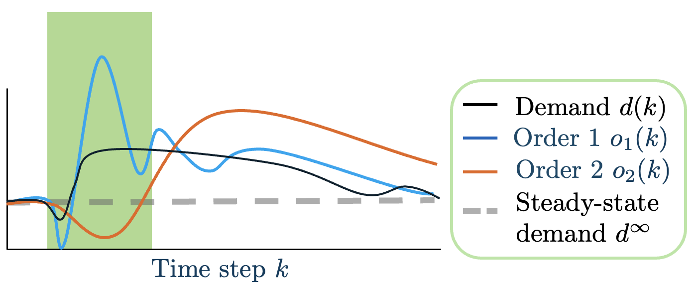
Figure 1: Comparing the transient behavior of two order schemes, $o_{1}(k)$ and $o_{2}(k)$, under the same demand fluctuations $d(k)-d^{\infty}$.

Evaluating $W_{E}$ (14) for the order series $o_{1}$ and $o_{2}$, we observe that the first order series $o_{1}(k)$ returns to the steady-state value much faster than the second order series $o_{2}(k)$, therefore $W_{E}(o_{1})<W_{E}(o_{2})$. However, $\max_{k}|o_{1}(k)-o^{\infty}|>\max_{k}|o_{2}(k)-o^{\infty}|$, and during the time period highlighted in green, $|o_{1}(k)-o^{\infty}|$ fluctuates significantly more than $|o_{2}(k)-o^{\infty}|$. We conclude that $o_{2}(k)$ creates higher transient virtual demand than $o_{1}(k)$ despite scoring lower on the metric $W_{E}$ (14).

As shown in Example 2, controllers that minimize the energy-based metric $W_{E}$ (14) can create higher transient order fluctuations despite scoring lower. This can be problematic for supply chain logistics, where a vendor’s ability to handle transient supply and demand fluctuations is bound by hard constraints arising from warehouse sizing and transportation availability. Furthermore, transient order fluctuations can cause excess stock and perceived shortages which, even if they are transient, can cascade into chain-wide disruptions such as those observed during the pandemic [12, 1]. To deal with these transient but potentially damaging order fluctuations, we propose an alternative metric that evaluates the transient energy transfer from demand fluctuations and forecast error to order fluctuations.

Definition 1 (Transient Bullwhip Measure).

The inventory dynamics (11) under the forecast-driven affine controller (12) and demand and forecast fluctuations $\mathcal{W}$ (13) have a transient Bullwhip measure given by

$$W_{T}=\underset{w(k)\in\mathcal{W},k\in\mathbb{N}}{\sup}|o(k)-o^{\infty}|.$$ (15)

The transient Bullwhip measure is the $\ell_{\infty}$ gain of $u(k)$ from (11) [20]. In contrast to the energy-based metric $\mathcal{W}_{E}$ (14), $\mathcal{W}_{T}$ (15) bounds the worst-case transient behavior of the vendor’s order dynamics. When applied to the two different order schemes from Example 2, the $W_{T}$ of $o_{2}$ will be lower than the $W_{T}$ of $o_{1}$, thus more accurately reflecting the potential damage caused by order fluctuations and the stress on the supply chain logistics.

III-A Bounding the transient Bullwhip measure

In general, the transient Bullwhip measure $W_{T}$ (15) can be difficult to compute. Instead, we build an upper bound for it using inescapable ellipsoids [21].

Definition 2 (Inescapable ellipsoid).

For a positive definite matrix $P\in{\mathbb{R}}^{n\times n}$, the set $\Phi(P)=\{x\in{\mathbb{R}}^{n}\ |\ x^{\top}Px\leq 1\}$ is an inescapable ellipsoid of the dynamics (11) under state feedback controller $F_{x}$ and forecast-driven controller $F_{w}$ if

1. $0\in\Phi(P)$

2. $x(k)\in\Phi(P)$ for all $w(k)\in\mathcal{W}$ when $x(0)\in\Phi(P)$.

The inescapable ellipsoid is a type of a robust positively invariant set [22], and can be used to bound the worst-case order peak gain achieved by any disturbance $w\in\mathcal{W}$ and initial state $x(0)\in\Phi(P)$, which is given by

$$\max_{x(k)\in\Phi(P),w(k)\in\mathcal{W}}\left\lVert F_{x}x(k)+F_{w}w(k)\right\rVert_{\infty}.$$ (16)

All inescapable sets provide an upper bound on $W_{T}$ [21]. Therefore, we approximate the transient Bullwhip measure via the tightest upper bound available using ellipsoid sets $\Phi(P)$, given by

$$W_{T}\leq\inf_{{P}\in\mathcal{S}_{++}^{n}}\max_{x\in\Phi({P}),w(k)\in{\mathcal{W}}}\left\lVert F_{x}x(k)+F_{w}w(k)\right\rVert_{\infty}.$$ (17)

We first normalize the tightest upper bound (17) to forecast errors and demand deviations in the disturbance set $\mathcal{W}$ (13).

Lemma 2.

We define the scaled disturbance set as

$$\hat{\mathcal{W}}=\left\{\frac{1}{\hat{\epsilon}}{w}\ |\ w\in\mathcal{W}~{}\eqref{eqn:forecast_and_demand_flux}\right\},$$ (18)

where $\hat{\epsilon}=\sqrt{\epsilon_{f}^{2}+(\epsilon_{d}+\epsilon_{f})^{2}}$. The transient Bullwhip measure (15) is upper-bounded by

$$W_{T}\leq\hat{\epsilon}\inf_{\hat{P}\in\mathcal{S}_{++}^{n}}\max_{x\in\Phi(\hat{P}),w(k)\in\hat{\mathcal{W}}}\left\lVert F_{x}x(k)+F_{w}w(k)\right\rVert_{\infty}.$$ (19)

Proof.

Let $x=\hat{\epsilon}\hat{x}$, ${w}=\hat{\epsilon}\hat{w}$. It follows that

1. $\hat{x}(k+1)=(A+BF_{x})\hat{x}(k)+(B_{w}+BF_{w})\hat{w}(k)$ if and only if ${x}(k+1)=(A+BF_{x}){x}(k)+(B_{w}+BF_{w}){w}(k)$;

2. $w^{\top}w\leq\hat{\epsilon}^{2}$ if and only if $\hat{w}^{\top}\hat{w}\leq 1$;

3. $x^{\top}Px\leq 1$ if and only if $\hat{x}^{\top}\hat{P}\hat{x}\leq 1$ where $\hat{P}=\hat{\epsilon}^{2}P$;

4. $\left\lVert F_{x}x(k)+F_{w}w(k)\right\rVert_{\infty}=\hat{\epsilon}\left\lVert F_{x}\hat{x}(k)+F_{w}\hat{w}(k)\right\rVert_{\infty}$.

We can conclude that the set $\Phi(P)$ is inescapable for the disturbance set $\mathcal{W}$ if and only if $\Phi(\hat{P})$ is inescapable for the disturbance set $\hat{\mathcal{W}}$. Furthermore,

$$\max_{\begin{subarray}{c}x(k)\in\Phi(P),\\ w(k)\in\mathcal{W}\end{subarray}}\left\lVert F_{x}x(k)+F_{w}w(k)\right\rVert_{\infty}=\\ \hat{\epsilon}\max_{\begin{subarray}{c}\hat{x}(k)\in\Phi(\hat{P}),\\ \hat{w}(k)\in\hat{\mathcal{W}}\end{subarray}}\left\lVert F_{x}\hat{x}(k)+F_{w}\hat{w}(k)\right\rVert_{\infty}.$$ (20)

Then the problem of finding the minimum upper bound on the transient Bullwhip measure $W_{T}$ is equivalent to (19). ∎

We first recall that checking whether a set $\Phi(P)$ is inescapable can be reduced to a bilinear matrix inequality condition.

Theorem 1.

[23, Thm.1] Consider the linear system (11) and the disturbance set $\hat{\mathcal{W}}$ (18). The ellipsoid $\Phi(P)$ is inescapable under the controllers $F_{x}=YP$ and $F_{w}$ if there exists a scalar value $\lambda\geq 0$ such that

$$\begin{bmatrix}-Q+\lambda Q&0&QA^{\top}+Y^{\top}B^{\top}\\ 0&-\lambda I&B_{w}^{\top}+{F}_{w}^{\top}B^{\top}\\ AQ+BY&B_{w}+B{F}_{w}&-Q\end{bmatrix}\preceq 0,Q=P^{-1},$$ (21)

where $F_{w}\in{\mathbb{R}}^{1\times 2}$ is the forecast-driven control matrix (12).

Next we show that given $P$, we can compute $\max_{x\in\Phi({P}),w(k)\in\hat{\mathcal{W}}}\left\lVert F_{x}x(k)+F_{w}w(k)\right\rVert_{\infty}$ via a second linear matrix inequality. Whereas this matrix inequality is typically expressed as a bilinear matrix inequality [21, 23], the structure of our forecast-driven affine controller enables the bilinear term to be reduced to a linear term, thus resulting in a linear matrix inequality.

Theorem 2.

Under the state feedback controller $F_{x}=YP$ and the forecast-driven controller $\frac{1}{\sqrt{\sigma}}F_{w}$, the $\ell_{\infty}$ gain of the order fluctuations $o(k)-o^{\infty}$ over the inescapable ellipsoid $\Phi(P)$ and disturbances $\hat{\mathcal{W}}$ (18) is upper bounded as

$$\max_{x\in\Phi(P),w(k)\in\hat{\mathcal{W}}}\left\lVert YPx(k)+\frac{1}{\sqrt{\sigma}}F_{w}w(k)\right\rVert_{\infty}\leq\gamma,$$ (22)

if and only if there exists a symmetric positive definite matrix $P$, $\lambda\geq 0$, such that (21) holds and there exists $\sigma,\gamma>0$ such that

$$\begin{bmatrix}Q&0&F_{x}^{\top}\\ 0&(\gamma^{2}-\sigma)I&F_{w}^{\top}\\ F_{x}&F_{w}&\sigma I\end{bmatrix}\succ 0,\ Q=P^{-1}.$$ (23)

Proof.

From [21, Lem.4.3], the two norm of the order peak under the forecast-driven affine controllers $F_{x}=YP,\hat{F}_{w}$ satisfies

$$\max_{x(k)^{\top}Px(k)\leq 1,w(k)^{\top}w(k)\leq 1}\left\lVert YPx(k)+\hat{F}_{w}w(k)\right\rVert^{2}_{2}\leq\gamma^{2},$$ (24)

if and only if there exists $0<\sigma$, such that

$$M=\begin{bmatrix}\sigma P&0&F_{x}^{\top}\\ 0&(\gamma^{2}-\sigma)I&\hat{F}_{w}^{\top}\\ F_{x}&\hat{F}_{w}&I\end{bmatrix}\succ 0.$$ (25)

We substitute $F_{x}=YP$ and left and right multiply $M$ by $S_{1}=\mathop{\bf diag}\{Q,I,I\}$. Since $S_{1}\succ 0$, $S_{1}MS_{1}\succ 0$,

$$S_{1}MS_{1}=\begin{bmatrix}\sigma Q&0&Y^{\top}\\ 0&(\gamma^{2}-\sigma)I&\hat{F}_{w}^{\top}\\ Y&\hat{F}_{w}&I\end{bmatrix}\succ 0.$$ (26)

From Schur complement, (26) holds if and only if

$$S_{1}MS_{1}=\begin{bmatrix}(\gamma^{2}-\sigma)I&\hat{F}_{w}^{\top}\\ \hat{F}_{w}&I\end{bmatrix}-\begin{bmatrix}0&0\\ 0&\frac{1}{\sigma}YQ^{-1}Y^{\top}\end{bmatrix}\succ 0.$$ (27)

Again, we left and right multiply $S_{1}MS_{1}$ by $S_{2}=\mathop{\bf diag}\{I,\sqrt{\sigma}I\}$. Since $S_{2}\succ 0$, $S_{2}S_{1}MS_{1}S_{2}\succ 0$.

$$S_{2}S_{1}MS_{1}S_{2}=\begin{bmatrix}(\gamma^{2}-\sigma)I&\sqrt{\sigma}\hat{F}_{w}^{\top}\\ \sqrt{\sigma}\hat{F}_{w}&\sigma I\end{bmatrix}-\begin{bmatrix}0&0\\ 0&YQ^{-1}Y^{\top}\end{bmatrix}\succ 0.$$ (28)

We use Schur complement again to derive that $S_{2}S_{1}MS_{1}S_{2}\succ 0$ if and only if

$$\begin{bmatrix}Q&0&Y^{\top}\\ 0&(\gamma^{2}-\sigma)I&\sqrt{\sigma}\hat{F}_{w}^{\top}\\ Y&\sqrt{\sigma}\hat{F}_{w}&\sigma I\end{bmatrix}\succ 0.$$ (29)

Let $\hat{F}_{w}=\frac{1}{\sqrt{\sigma}}F_{w}$ and noting that $F_{x}{x}(k)+\frac{1}{\sqrt{\sigma}}F_{w}{w}(k)$ is a real number, $\left\lVert F_{x}{x}(k)+\frac{1}{\sqrt{\sigma}}F_{w}{w}(k)\right\rVert_{2}=\left\lVert F_{x}{x}(k)+\frac{1}{\sqrt{\sigma}}F_{w}{w}(k)\right\rVert_{\infty}$. ∎

As shown in [21], finding the $\ell_{\infty}$ gain without forecast-driven control involves solving a bilinear matrix inequality, which the authors reduced to solving an algebraic Riccati equation and a linear matrix inequality. Using the forecast-driven affine controller (1), we can avoid solving an algebraic Riccati equation.

IV Bullwhip-minimizing feedback control design

From Theorems 1 and 2, we can conclude that the forecast-driven affine controller that provides the tightest upper-bound on the transient Bullwhip measure $W_{T}$ (15) via inescapable ellipsoids is the optimal argument to the following optimization problem with bilinear matrix inequality constraints.

$$W_{T}\leq \inf_{\lambda,Q,\sigma,Y,\gamma,F_{w}}\hat{\epsilon}\gamma$$ (30)

s.t. $$\begin{bmatrix}-Q+\lambda Q&0&QA^{\top}+YB^{\top}\\ 0&-\lambda I&B_{w}^{\top}+\hat{F}_{w}^{\top}B^{\top}\\ AQ+BY&B_{w}+B\hat{F}_{w}&-Q\end{bmatrix}\preceq 0$$ (31)

$$\begin{bmatrix}Q&0&Y^{\top}\\ 0&(\gamma^{2}-\sigma)I&\hat{F}_{w}^{\top}\\ Y&\hat{F}_{w}&\sigma I\end{bmatrix}\succ 0$$ (32)

$$Q\succ 0,\sigma,\gamma>0,\hat{F}_{w}=\begin{bmatrix}0&F_{w}&0\end{bmatrix}^{\top}.$$ (33)

With optimal values $\gamma^{\star}$ and optimal arguments $Q^{\star},\sigma^{\star},Y^{\star},F_{w}^{\star}$, the peak gain minimizing control is given by $u(k)=Y^{\star}(Q^{\star})^{-1}x(k)+\frac{1}{\sqrt{\sigma^{\star}}}F^{\star}_{w}w_{2}(k)$ and the minimal peak gain is given by $\gamma^{\star}\sqrt{\epsilon_{f}^{2}+(\epsilon_{f}+\epsilon_{d})^{2}}$.

The optimization problem (30) is non-convex due the existence of a bilinear matrix term $\lambda Q$ in (31). We consider the following function whose point-wise values are semi-definite programs,

$$f(\lambda)= \min_{Q,\lambda,\sigma,Y,F_{w}}\gamma^{2}$$ (34)

s.t. $$\begin{bmatrix}-Q+\lambda Q&0&QA^{\top}+YB^{\top}\\ 0&-\lambda I&B_{w}^{\top}+F_{w}^{\top}B^{\top}\\ AQ+BY&B_{w}+BF_{w}&-Q\end{bmatrix}\preceq 0$$

$$\begin{bmatrix}Q&0&Y^{\top}\\ 0&(\gamma^{2}-\sigma)I&F_{w}^{\top}\\ Y&F_{w}&\sigma I\end{bmatrix}\succ 0$$

$$Q\succ 0,\sigma,\gamma>0.$$

We first show that this function is only well defined on the interval $\lambda\in(0,1]$.

Lemma 3.

The function $f(\lambda)$ (34) not well-defined for $\lambda<0$ or $\lambda>1$. On $\lambda\in(0,1]$, $f(\lambda)$ is quasi-convex.

Proof.

To see that $\lambda>1$ and $\lambda<0$ result in infeasible LMIs, we first note that a necessary condition for an LMI to be negative semi-definite is that its diagonal matrices and principal minors must be negative semi-definite. In particular, this implies that $(\lambda-1)Q\preceq 0$ and $-Q\preceq 0$. When $\lambda>1$, $Q$ must be $0$ to satisfy both conditions. When $\lambda<0$, the $(2,2)$ element of the first LMI constraint, $-\lambda I$, cannot be negative semidefinite.

When $\lambda\in(0,1]$, let $F_{w},Y$ both be the $0$ matrices in their respective dimensions, we can find a set of $Q$’s for which the LMIs are feasible using the Schur complement

$$\begin{bmatrix}(\lambda-1)Q&0&QA^{\top}\\ 0&-\lambda I&B_{w}^{\top}\\ AQ&B_{w}&-Q\end{bmatrix}\preceq 0\leftrightarrow\\ -Q-\begin{bmatrix}AQ&B_{w}\end{bmatrix}\begin{bmatrix}\frac{1}{\lambda-1}Q^{-1}&0\\ 0&-\frac{1}{\lambda}I\end{bmatrix}\begin{bmatrix}QA^{\top}\\ B^{\top}_{w}\end{bmatrix}\preceq 0\leftrightarrow\\ -Q-\frac{1}{\lambda-1}AQA^{\top}+\frac{1}{\lambda}B_{w}B_{w}^{\top}\preceq 0.$$ (35)

Then let $Q=I+\frac{1}{\lambda}B_{w}B_{w}^{\top}$ and the resulting LMI (35) will be satisfied. This also holds when $\lambda=1$, where the corresponding LMI is given by $-Q+\frac{1}{\lambda}B_{w}B_{w}^{\top}\preceq 0.$ The result that $f(\lambda)$ is quasi-convex when $f(\lambda)$ is well-defined follows from the proof of [21, Thm.3.2]. ∎

Given that $f(\lambda)$ is quasi-convex, we can perform a bisection search on $\lambda\in(0,1]$ to find $\min_{\lambda}f(\lambda)$. However, our empirical results in the following section indicate that the minimum $f(\lambda)$ occurs at $\lim_{\lambda\rightarrow 0}f(\lambda)$, and $f(\lambda)$ is only sensitive to $\lambda$ for non-perishable commodities $\beta\sim 0$.

V Empirical observations on gain sensitivity and controller performance

We evaluate the quasi-convex function (34) for different perishing and backlogging rates on the domain $\lambda=[0,1]$. We also compare the peak-gain minimizing controller’s properties including its reliance on the forecast and its performance under different forecast oracles.

V-A Impact of backlog and perishing rates

We first let $\hat{\epsilon}=1$ (18) and evaluate the peak gain $\gamma=\sqrt{f(\lambda)}$ (34) for different combinations of perishable rates $\beta$ and backlog rates $\alpha$ over $\lambda\in(0,1)$. The results are shown in Figures 2 and 3. We observe that $f(\lambda)$ does indeed vary with $\lambda$. Based on our empirical results, $f(\lambda)$ appears to be a monotonic function that strictly increases in $\lambda$ for all sampled combinations of backlog and perishing rates. Furthermore, $f(\lambda)$ appears to be continuous overall but runs into computation issues when $f(\lambda)\sim 1e-8$, which may be occurring due to numerical computation errors.

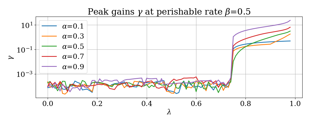
Figure 2: Peak gains $\sqrt{f(\lambda)}$ as a function of $\lambda$ for perishing rate $\beta=0.5$ and varying backlog rates.

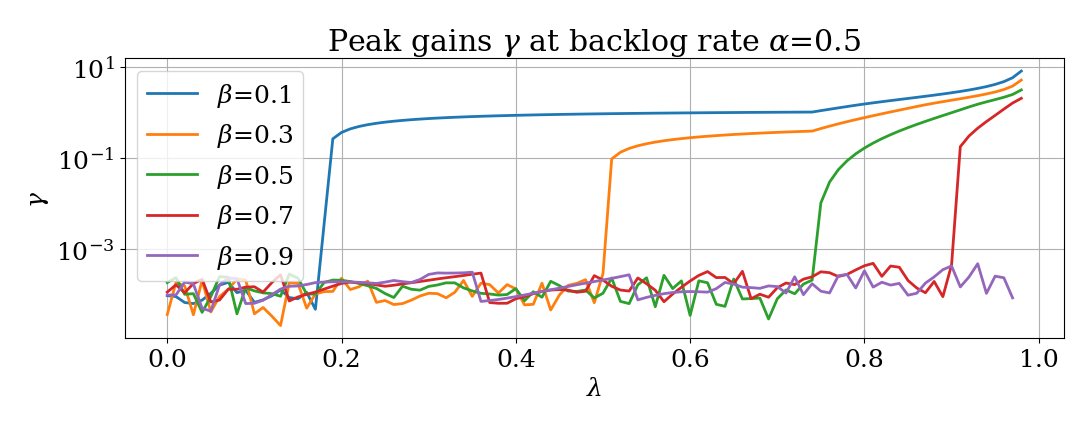
Figure 3: Peak gains $\sqrt{f(\lambda)}$ as a function of $\lambda$ for backlog rate $\alpha=0.5$ and varying perish rates.

From Figure 2, we observe that the peak gain $\sqrt{f(\lambda)}$ drops significantly around $\lambda\simeq 0.7$ for different backlog rates $\alpha$, while in Figure 3, we observe that the same drop in the peak gain $\sqrt{f(\lambda)}$ occurs at different values of $\lambda$, such that the drop occurs at lower $\lambda$ values when $\beta$ increases. Combining these observations together, we note that empirically, the backlog rate does not significantly influence the region of $\lambda$ over which the minimum peak gain occurs, while a lower perishing rate $\beta$ causes the minimum peak gain $\gamma^{\star}$ to be more sensitive $\lambda$, and that in general, evaluating $\sqrt{f(\lambda)}$ at $\lambda$ values close to $0$ could result in better approximations of the minimum peak gain. Interestingly, we observe from both Figure 2 and 3 that neither the backlog nor the perishing rate affects the minimum peak gain value $\min_{\lambda}\sqrt{f(\lambda)}$ near $\lambda=0$. For supply chains, this empirical observation may imply that all different backlogging and perishing rate combinations have forecast-driven affine controllers that can drive their peak gains very close to zero.

V-B Controller performance under different forecast oracles

Next, we evaluate the peak-minimizing controller’s performance for the inventory dynamics (11) with perishing rate $\beta=0.1$, and backlog rate $\alpha=0.1$. We compute $f(0.01)$ (34), and use the resulting controllers $F_{x}^{\star}$ and $F_{w}^{\star}$ for the forecast and demand uncertainty set $\mathcal{W}$ (13), with different demand and forecast errors, $\epsilon_{d}=1000$ and $\epsilon_{f}\in[0,1000]$, respectively. We evaluate the resulting closed-loop dynamics for random initial conditions for $1000$ time steps and observe the maximum fluctuation in order and inventory. The results are shown in Figures 4 and 5.

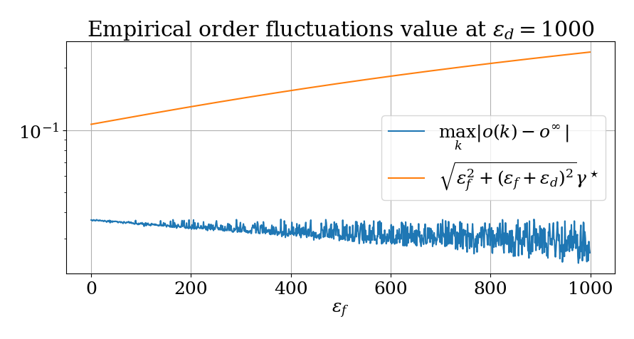
Figure 4: Maximum empirical order fluctuations over $1000$ timesteps as a function of increasing forecast error, $\epsilon_{f}\in[0,\epsilon_{d}]$. We note that the empirical order fluctuation (blue) hovers around a maximum of $0.04$ and the theoretical bound $\gamma^{\star}\sqrt{\epsilon_{f}^{2}+(\epsilon_{f}+\epsilon_{d})^{2}}$ monotonically increases from $0.1$ to about $0.2$.

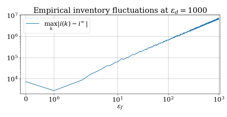
Figure 5: Maximum empirical inventory fluctuations over $1000$ timesteps as a function of increasing forecast error, $\epsilon_{f}\in[0,\epsilon_{d}]$.

We observe from Figure 4 that the maximum order fluctuation is well within the range predicted by the predicted transient Bullwhip value, shown in orange. This may imply that our worse-case upper bound is overly conservative. Furthermore, it appears that the maximum empirical order fluctuation is around $0.04$ for all values of $\epsilon_{f}$. However, we note that we are sampling randomly and not computing the worst-case scenario.

Interestingly, while forecast error did not appear to impact the empirical order fluctuations, it did significantly impact the empirical inventory fluctuations (shown in Figure 5, with the inventory fluctuations reaching $10e6$ for $\epsilon_{f}\simeq 0.2\epsilon_{d}$, a fairly accurate forecast oracle that is able to reduce the future demand uncertainty five-fold. Finally, we note that the trend for inventory fluctuation is not strictly monotone. At zero forecast error, the empirical inventory fluctuations in fact increased. We repeatedly observed this slight increase at zero forecast error for all repeated trials.

VI Conclusion

In this paper, we developed a new measure for the transient Bullwhip effects using the $\ell_{\infty}$ gain of a forecast-driven affine control model of a single commodity supply chain vendor. We showed that the resulting peak gain can be upper-bounded by a quasi-convex function defined within the domain $\lambda\in(0,1]$, and whose point-wise value is the minimal value of an LMI-constrained optimization problem. Future work includes extending the model to consider multi-vendor supply chains to further understand the role of individual forecast errors on the Bullwhip effect.

References

- [1] V. Yee and J. Glanz, “How one of the world’s biggest ships jammed the suez canal,” The New York Times. [Online]. Available: https://www.nytimes.com/2021/07/17/world/middleeast/suez-canal-stuck-ship-ever-given.html
- [2] S. M. Wagner and C. Bode, “An empirical investigation into supply chain vulnerability,” Journal of purchasing and supply management, vol. 12, no. 6, pp. 301–312, 2006.
- [3] V. Ranganathan, P. Kumar, U. Kaur, S. H. Li, T. Chakraborty, and R. Chandra, “Re-inventing the food supply chain with iot: A data-driven solution to reduce food loss,” IEEE Internet of Things Magazine, vol. 5, no. 1, pp. 41–47, 2022.
- [4] H. L. Lee, V. Padmanabhan, and S. Whang, “The bullwhip effect in supply chains,” 1997.
- [5] X. Zhang, “The impact of forecasting methods on the bullwhip effect,” International journal of production economics, vol. 88, no. 1, pp. 15–27, 2004.
- [6] C.-Y. Chiang, W. T. Lin, and N. C. Suresh, “An empirically-simulated investigation of the impact of demand forecasting on the bullwhip effect: Evidence from us auto industry,” International Journal of Production Economics, vol. 177, pp. 53–65, 2016.
- [7] F. Chen, J. K. Ryan, and D. Simchi-Levi, “The impact of exponential smoothing forecasts on the bullwhip effect,” Naval Research Logistics (NRL), vol. 47, no. 4, pp. 269–286, 2000.
- [8] X. Wang and S. M. Disney, “The bullwhip effect: Progress, trends and directions,” European Journal of Operational Research, vol. 250, no. 3, pp. 691–701, 2016.
- [9] F. Costantino, G. Di Gravio, A. Shaban, and M. Tronci, “The impact of information sharing and inventory control coordination on supply chain performances,” Computers & Industrial Engineering, vol. 76, pp. 292–306, 2014.
- [10] Y. Ouyang and X. Li, “The bullwhip effect in supply chain networks,” European Journal of Operational Research, vol. 201, no. 3, pp. 799–810, 2010.
- [11] M. Udenio, E. Vatamidou, J. C. Fransoo, and N. Dellaert, “Behavioral causes of the bullwhip effect: An analysis using linear control theory,” Iise Transactions, vol. 49, no. 10, pp. 980–1000, 2017.
- [12] M. Lunsford, “Chicken wing shortage? another strange pandemic complication,” AP News. [Online]. Available: https://apnews.com/general-news-3b478b6531de4cc7d2bdc2d093c13340
- [13] T. N. Burrows, M. A. Hamilton, and D. Grimsman, “Who gets the whip? how supplier diversification influences bullwhip effect in a supply chain,” in 2023 62nd IEEE Conference on Decision and Control (CDC), 2023, pp. 7592–7597.
- [14] M. V. Khlebnikov, “Control of linear systems subjected to exogenous disturbances: Combined feedback,” IFAC-PapersOnLine, vol. 49, no. 13, pp. 111–116, 2016.
- [15] H. Zhang and J. Wang, “Combined feedback–feedforward tracking control for networked control systems with probabilistic delays,” Journal of the Franklin Institute, vol. 351, no. 6, pp. 3477–3489, 2014.
- [16] F. Constantino, G. Di Gravio, A. Shaban, and M. Tronci, “Exploring the bullwhip effect and inventory stability in a seasonal supply chain,” International Journal of Engineering Business Management, vol. 5, no. Godište 2013, pp. 5–23, 2013.
- [17] D. V. Gordon, “Price modelling in the canadian fish supply chain with forecasts and simulations of the producer price of fish,” Aquaculture economics & management, vol. 21, no. 1, pp. 105–124, 2017.
- [18] Y. Jin, B. D. Williams, T. Tokar, and M. A. Waller, “Forecasting with temporally aggregated demand signals in a retail supply chain,” Journal of Business Logistics, vol. 36, no. 2, pp. 199–211, 2015.
- [19] R. Carbonneau, K. Laframboise, and R. Vahidov, “Application of machine learning techniques for supply chain demand forecasting,” European journal of operational research, vol. 184, no. 3, pp. 1140–1154, 2008.
- [20] S. Boyd and J. Doyle, “Comparison of peak and rms gains for discrete-time systems,” Systems & control letters, vol. 9, no. 1, pp. 1–6, 1987.
- [21] J. Abedor, K. Nagpal, and K. Poolla, “A linear matrix inequality approach to peak-to-peak gain minimization,” International Journal of Robust and Nonlinear Control, vol. 6, no. 9-10, pp. 899–927, 1996.
- [22] F. Blanchini, “Set invariance in control,” Automatica, vol. 35, no. 11, pp. 1747–1767, 1999.
- [23] J. Xiao-Fu, S. Hong-Ye, and C. Jian, “Peak-to-peak gain minimization for uncertain linear discrete systems: A matrix inequality approach,” Acta Automatica Sinica, vol. 33, no. 7, pp. 753–756, 2007.