Debiased calibration estimation using generalized entropy in survey sampling

Abstract

Incorporating the auxiliary information into the survey estimation is a fundamental problem in survey sampling. Calibration weighting is a popular tool for incorporating the auxiliary information. The calibration weighting method of Deville and Särndal, (1992) uses a distance measure between the design weights and the final weights to solve the optimization problem with calibration constraints. This paper introduces a novel framework that leverages generalized entropy as the objective function for optimization, where design weights play a role in the constraints to ensure design consistency, rather than being part of the objective function. This innovative calibration framework is particularly attractive due to its generality and its ability to generate more efficient calibration weights compared to traditional methods based on Deville and Särndal, (1992). Furthermore, we identify the optimal choice of the generalized entropy function that achieves the minimum variance across various choices of the generalized entropy function under the same constraints. Asymptotic properties, such as design consistency and asymptotic normality, are presented rigorously. The results from a limited simulation study are also presented. We demonstrate a real-life application using agricultural survey data collected from Kynetec, Inc.

Keywords: Empirical likelihood, generalized regression estimation, selection bias.

1 Introduction

Many scientific studies rely on analyzing data sets that consist of samples from target populations. The fundamental assumption when using such data is that the sample accurately represents the target population, ensuring representativeness. Probability sampling is a classical tool for securing a representative sample from a target population. Once a probability sample is obtained, researchers can employ design-consistent estimation methods, such as Horvitz-Thompson estimation, to estimate the parameters of the population. Statistical inferences, such as confidence intervals, can be made from the probability sample using the large sample theory (Fuller,, 2009).

However, the Horvitz-Thompson (HT) estimator is not necessarily efficient in the sense that its variance can be large. How to improve the efficiency of the HT estimator is one of the fundamental problems in survey sampling. A classical approach to improving efficiency involves the use of additional information obtained from external sources, such as census data. To incorporate auxiliary information into the final estimate, the design weights are adjusted to meet the benchmarking constraints imposed by the auxiliary information. Such a weight modification method to satisfy the benchmarking constraint is known as calibration weighting. While calibration weighting also plays a role in mitigating selection bias in nonprobability samples, as highlighted by Dever and Valliant, (2016) and Elliott and Valliant, (2017), our discussion will focus on its application within probability samples.

The literature on calibration weighting is very extensive. Isaki and Fuller, (1982) used a linear regression superpopulation model to construct the regression calibration weights and showed that the resulting estimator is optimal in the sense that its anticipated variance achieves the lower bound of Godambe and Joshi, (1965). Deville and Särndal, (1992) developed a unified framework for calibration estimation and showed the asymptotic equivalence between the calibration estimator and the generalized regression (GREG) estimator. Wu and Sitter, (2001) explicitly utilized the regression model to develop what is known as model calibration. Breidt and Opsomer developed a series of nonparametric regression estimators (Breidt et al.,, 2005; Breidt and Opsomer,, 2017) that can be understood as nonparametric calibration weighting. Montanari and Ranalli, (2005) also developed a framework for nonparametric model calibration using neural network models. Dagdoug et al., (2023) employ random forest to develop a nonparametric model calibration. Devaud and Tillé, (2019) presented a comprehensive review of calibration weighting methods in survey sampling.

Most existing calibration weighting methods are grounded in the framework established by Deville and Särndal, (1992), which utilizes a distance measure between the design weights and the final weights to address the optimization problem within the calibration constraints. In this paper, we introduce an alternative approach that employs generalized entropy as an objective function for optimization. Here, design weights are incorporated into the constraints rather than the objective function to solve the calibration optimization problem. The constraint involving the design weights is designed to mitigate selection bias, whereas the benchmarking constraint aims to decrease variance. To differentiate between these two calibration constraints, the one that incorporates design weights is called the debiasing constraint, to emphasize its role in controlling the selection bias. Although generalized entropy has been developed as a tool for efficient estimation (Newey and Smith,, 2004), current literature lacks a discussion of the debiasing constraint under selection bias.

The idea of employing a debiasing constraint within the calibration weighting framework is not entirely new. Qin et al., (2002) is perhaps the first attempt to correct selection bias using empirical likelihood in the context of missing data. Berger and Torres, (2016) also employed debiasing constraints using empirical likelihood within the survey sampling context. Chapter 2 of Fuller, (2009) also discussed the incorporation of the debiasing constraint into the linear regression model. The objective of this paper is to generalize the idea further and introduce a unified framework for debiased calibration that aims to reduce selection bias and improve estimation efficiency in survey sampling scenarios. Our proposed methodology produces a design-consistent calibration estimator that is more efficient than the calibration estimator of Deville and Särndal, (1992) in general. Our approach is based on generalized entropy for optimization. Thus, the empirical likelihood approach of Qin et al., (2002) is a special case of our unified approach.

Based on asymptotic theory, we formally show that the cross-entropy function is the optimal entropy function in the sense that it attains the minimum variance among the different choices of the generalized entropy function under the same constraints. Thus, in addition to generality, we also present an important result for optimality. By imposing the debiasing constraint, we can improve the efficiency of the calibration estimator, especially when the sampling weights are informative in the sense of Pfeffermann and Sverchkov, (2009).

The debiasing constraint implicitly assumes that the design weights are available throughout the finite population. When design weights are not available outside the sample, the debiasing constraint cannot be used directly. In this case, we can treat the population mean of the debiased control as another unknown parameter and develop an efficient estimator using nonparametric regression or using a modification of the generalized entropy. More details are presented in Section 6.

The paper is organized as follows. In Section 2, the basic setup and the research problem are introduced. In Section 3, we present the proposed method using generalized entropy calibration and give an illustration using empirical likelihood as a special case. In Section 4, the asymptotic properties of the proposed method are rigorously derived, and a consistent variance estimator is also presented. In Section 5, we show that the optimal entropy function in the context of calibration estimation is achieved with the cross-entropy function. In Section 6, we present a modification of the proposed method when the design weights are not available outside the sample. Results of a limited simulation study are presented in Section 7. In Section 8, we demonstrate a real-life application using agricultural survey data collected from Kynetec. Some concluding remarks are made in Section 9. All the technical proofs are relegated to the supplementary material (SM).

2 Basic setup

Consider a finite population $U=\mathinner{\left\{1,\cdots,N\right\}}$ of $N$ units, with known $N$. A sample $A$ of size $n$ is selected from the finite population using a given probability sampling design. We use $\delta_{i}$ to denote the sampling indicator variable of unit $i$ such that $\delta_{i}=1$ if $i\in A$ and $\delta_{i}=0$ otherwise. We assume that first-order inclusion probabilities $\mathinner{\left\{\pi_{i}\mathrel{\mathop{\mathchar 58\relax}}i\in U\right\}}$ are available throughout the population. We will relax this assumption later in Section 6.

Let $y_{i}$ be the study variable of interest, available only in sample $A$. Our goal is to estimate the finite population total $\theta_{\rm N}=\sum_{i\in U}y_{i}=\sum_{i=1}^{N}y_{i}$ from sample $A$. We consider a class of linear estimator

$$\hat{\theta}=\sum_{i\in A}\omega_{i}y_{i}$$ (2.1)

where $\omega_{i}$ does not depend on $\mathinner{\left\{y_{i}\mathrel{\mathop{\mathchar 58\relax}}i\in A\right\}}$. The Horvitz-Thompson (HT) estimator is a natural way to estimate $\theta_{\rm N}$ using $\omega_{i}=\pi_{i}^{-1}$. The HT estimator is design-unbiased but can be inefficient.

In many practical situations, in addition to the study variable $y_{i}$, we observe $p$-dimensional auxiliary variables $\bm{x}_{i}=(x_{i1},\ldots,x_{ip})^{\top}$ with known population totals from external sources. In this case, to get external consistency, we often require that the final weights satisfy

$$\sum_{i\in A}\omega_{i}\bm{x}_{i}=\sum_{i\in U}\bm{x}_{i}.$$ (2.2)

Constraint (2.2) is often called a calibration constraint or a benchmarking constraint. Generally speaking, the calibration estimator is more efficient than the HT estimator when the study variable $y$ of interest is related to the auxiliary variable $\bm{x}$. However, the calibration estimator that satisfies (2.2) is not necessarily design-consistent.

To achieve the design consistency of the calibration estimator, Deville and Särndal, (1992) proposed solving an optimization problem that minimizes the distance between the calibration weights $\bm{\omega}=\mathinner{\left(\omega_{i}\right)}_{i\in A}$ and the design weights $\bm{d}=\mathinner{\left(\pi_{i}^{-1}\right)}_{i\in A}$

$$D(\bm{\omega},\bm{d})=\sum_{i\in A}d_{i}G(\omega_{i}/d_{i})$$ (2.3)

subject to the calibration constraints in (2.2), where $d_{i}=\pi_{i}^{-1}$ for $i\in A$ and $G(\cdot)\mathrel{\mathop{\mathchar 58\relax}}\mathcal{V}\to\mathbb{R}$ is a nonnegative function that is strictly convex, differentiable, and $G^{\prime}(1)=0$. The domain $\mathcal{V}$ of $G(\cdot)$ is an open interval in $\mathbb{R}$. The distance measure $D(\bm{\omega},\bm{d})$ in (2.3) serves as the divergence between two discrete measures $\bm{\omega}$ and $\bm{d}$. For example, $G(\omega)=\omega\log(\omega)-\omega+1$, with domain $\mathcal{V}\subseteq(0,\infty)$, corresponds to the Kullback-Leibler divergence, while $G(\omega)=(\omega-1)^{2}$, with the domain $\mathcal{V}\subseteq(-\infty,\infty)$, corresponds to the Chi-squared distance from 1.

Let $\hat{\omega}_{{\rm DS},i}$ be the solution to the above optimization problem, and let $\hat{\theta}_{\rm DS}=\sum_{i\in A}\hat{\omega}_{{\rm DS},i}y_{i}$ be the resulting estimator. Under some conditions on $G(\cdot)$, $\hat{\theta}_{\rm DS}$ is asymptotically equivalent to the generalized regression (GREG) estimator given by

$$\hat{\theta}_{\rm greg}=\sum_{i\in U}\bm{x}_{i}^{\top}\hat{\bm{\beta}}+\sum_{i\in A}d_{i}(y_{i}-\bm{x}_{i}^{\top}\hat{\bm{\beta}})$$ (2.4)

where

$$\hat{\bm{\beta}}=\bigg{(}\sum_{i\in A}d_{i}\bm{x}_{i}\bm{x}_{i}^{\top}\bigg{)}^{-1}\sum_{i\in A}d_{i}\bm{x}_{i}y_{i}.$$ (2.5)

Note that the GREG estimator in (2.4) can be expressed as the sum of two terms; the prediction term and the bias correction term. The bias correction term is calculated from the sample using the HT estimation of the bias of the prediction estimator. The bias-corrected prediction estimator is also called a debiased prediction estimator in the causal inference literature (Athey et al.,, 2018). The debiasing property comes from the fact that the objective function in (2.3) is minimized at $\omega_{i}=d_{i}$ when the calibration constraints are already satisfied with the design weights. When the sample size is sufficiently large, by the law of large numbers, the calibration constraints are nearly satisfied with the design weights. Thus, the final calibration weights should converge to the design weights as the sample size increases.

Although the bias correction term has the clear advantage of eliminating bias, it can have the disadvantage of increasing variance because the bias term is estimated by the HT estimation method. In the following sections, we propose another approach to the debiased calibration estimator that is more efficient than the classical calibration estimator that uses (2.3). The basic idea is to incorporate bias correction into the calibration constraint, which will be called a debiasing constraint. That is, we can simply use debiasing and benchmarking constraints in the calibration weighting. The debiasing constraint is to control the selection bias, while the benchmarking constraint is to control the efficiency. The use of a debiasing constraint in calibration weighting is similar in spirit to interval bias calibration (IBC) in prediction estimation (Firth and Bennett,, 1998). The debiasing constraint in the calibration estimator plays the role of IBC in the prediction estimator.

3 Methodology

Instead of minimizing the weight distance measure in (2.3), we now consider maximizing the generalized entropy (Gneiting and Raftery,, 2007) that does not depend on the design weights:

$$H(\bm{\omega})=-\sum_{i\in A}G(\omega_{i})$$ (3.1)

where $G(\cdot)\mathrel{\mathop{\mathchar 58\relax}}\mathcal{V}\to\mathbb{R}$ is a strictly convex and differentiable function and $\bm{\omega}$ denotes the vector of $\{\omega_{i}\mathrel{\mathop{\mathchar 58\relax}}i\in A\}$. Note that the function $G(\cdot)$ in (3.1) is more general than that in (2.3). It does not need to be nonnegative or satisfy $G^{\prime}(1)=0$ as in (2.3). The empirical likelihood is a special case of (3.1) with $G(\omega_{i})=-\log\omega_{i}$, while the Shannon-entropy uses $G(\omega_{i})=\omega_{i}\log\omega_{i}$.

To incorporate design information and guarantee design consistency, in addition to the benchmarking covariates calibration constraints in (2.2), we add the following design calibration constraint

$$\sum_{i\in A}\omega_{i}g(d_{i})=\sum_{i\in U}g(d_{i}),$$ (3.2)

where $g(\omega)=dG(\omega)/d\omega$ denotes the first-order derivative of $G(\cdot)$. The constraint in (3.2) is the key constraint to make the proposed calibration estimator in (3.4) design consistent, which is called the debiasing calibration constraint.

Let $\bm{z}_{i}^{\top}=(\bm{x}_{i}^{\top},g(d_{i}))\in\mathbb{R}^{p+1}$. We wish to find the calibration weights $\bm{\omega}$ that maximize the generalized entropy in (3.1) under the calibration constraints in (2.2) and (3.2) so that the resulting weighted estimator is design consistent and efficient. The optimization problem of interest can be formulated as follows

$$\hat{\bm{\omega}}=\operatorname*{arg\,min}_{\bm{\omega}\in\Omega_{A}\cap\mathcal{V}^{n}}\sum_{i\in A}G(\omega_{i})\mbox{ \ for \ }\Omega_{A}=\bigg{\{}\bm{\omega}=\mathinner{\left(\omega_{i}\right)}_{i\in A}\mathrel{\mathop{\mathchar 58\relax}}\sum_{i\in A}\omega_{i}\bm{z}_{i}=\sum_{i\in U}\bm{z}_{i}\bigg{\}},$$ (3.3)

where $\hat{\bm{\omega}}$ is the vector of $\{\hat{\omega}_{i}\mathrel{\mathop{\mathchar 58\relax}}i\in A\}$. Using the calibration weights $\hat{\bm{\omega}}$, the proposed calibration estimator of the population total $\theta_{\rm N}$ is constructed as

$$\hat{\theta}_{\rm cal}=\sum_{i\in A}\hat{\omega}_{i}y_{i}.$$ (3.4)

Let $F(\omega)=-G(g^{-1}(\omega))+g^{-1}(\omega)\omega$ be the convex conjugate function of $G(\omega)$. Let $f(\omega)=dF(\omega)/d\omega$ be the first-order derivative of $F(\omega)$, and $g(\mathcal{V})$ denote the range of $g(\omega)$ over the domain $\omega\in\mathcal{V}$. It can be shown that $f(\omega)=g^{-1}(\omega)$. The primal problem in (3.3) can be formulated as a dual problem

$$\hat{\bm{\lambda}}=\operatorname*{arg\,min}_{\bm{\lambda}\in\Lambda_{A}}\sum_{i\in A}F(\bm{\lambda}^{\top}\bm{z}_{i})-\bm{\lambda}^{\top}\sum_{i\in U}\bm{z}_{i},$$ (3.5)

where $\hat{\bm{\lambda}}=(\hat{\bm{\lambda}}_{1}^{\top},\hat{\lambda}_{2})^{\top}$ and $\Lambda_{A}=\big{\{}\bm{\lambda}\mathrel{\mathop{\mathchar 58\relax}}\bm{\lambda}^{\top}\bm{z}_{i}\in g(\mathcal{V})\mbox{ \ for all \ }i\in A\big{\}}$. Solutions to (3.3) and (3.5) satisfy

$$\hat{\omega}_{i}=\hat{\omega}_{i}(\hat{\bm{\lambda}})=f(\hat{\bm{\lambda}}^{\top}\bm{z}_{i})=g^{-1}\{\hat{\bm{\lambda}}_{1}^{\top}\bm{x}_{i}+\hat{\lambda}_{2}g(d_{i})\}.$$ (3.6)

While $\bm{\omega}$ is $n$-dimensional, $\bm{\lambda}$ is $(p+1)$-dimensional, which implies that the dual optimization problem in (3.5) is easier to compute compared to the primal problem of (3.3).

The expression of $\hat{\omega}_{i}$ in (3.6) helps to understand the role of the design calibration constraint (3.2) in the proposed procedure. For a sufficiently large sample size, the calibration equations in (2.2) and (3.2) will be satisfied with $\hat{\omega}_{i}=d_{i}=\pi_{i}^{-1}$ with probability approaching one. This implies that the probability limit of the calibration weight $\hat{\omega}_{i}$ should be equal to the design weight $d_{i}$. From the expression of $\hat{\omega}_{i}(\hat{\bm{\lambda}})$ in (3.6), this is true when $\hat{\bm{\lambda}}_{1}\to{\bm{0}}$ and $\hat{\lambda}_{2}\to 1$ in probability. Therefore, by including the constraint in (3.2), we can establish the design consistency of the proposed calibration estimator $\hat{\theta}_{\rm cal}$. A theoretical justification of the design consistency property of the proposed estimator is presented in the next section.

Deville and Särndal, (1992) showed that the calibration weights $\hat{\omega}_{{\rm DS},i}$ using the divergence measure in (2.3) can be expressed as

$$\hat{\omega}_{{\rm DS},i}=\hat{\omega}_{{\rm DS},i}(\hat{\bm{\lambda}}_{\rm DS,1})=d_{i}g^{-1}(\hat{\bm{\lambda}}_{\rm DS,1}^{\top}\bm{x}_{i})$$ (3.7)

where $\hat{\bm{\lambda}}_{\rm DS,1}$ is the Lagrange multiplier to make the weights $\{\hat{\omega}_{{\rm DS},i}(\hat{\bm{\lambda}}_{\rm DS,1})\}_{i\in A}$ satisfy the calibration constraints in (2.2). It can be shown that $\hat{\bm{\lambda}}_{\rm DS,1}$ converges to zero as the sample size increases to infinity. By comparing (3.6) with (3.7), we can see that the main distinction between the divergence calibration method in Deville and Särndal, (1992) and the proposed entropy calibration approach is in the way that the selection probabilities $\{d_{i}\}$ are utilized. The divergence calibration method uses $\{d_{i}\}$ of the sampled units only, which are incorporated directly into the objective function. However, the proposed method uses the selection probabilities in the entire population by imposing the debiasing calibration constraint in (3.2). An additional parameter $\lambda_{2}$ is introduced to adjust the effect of the design weight $d_{i}$.

In the case where the design weights $\{\pi_{i}\mathrel{\mathop{\mathchar 58\relax}}i\not\in A\}$ are not available, we can treat $\sum_{i\in U}g(d_{i})$ as an unknown parameter and estimate it from the sample. See Section 6 for more discussion.

Empirical Likelihood Example. The empirical likelihood (Owen,, 1988) objective function of (3.1) uses $G(\omega)=-\log(\omega)$. Since $g(\omega)=-\omega^{-1}$ in this case, the debiasing constraint in (3.2) takes the form $\sum_{i\in A}\omega_{i}\pi_{i}=\sum_{i\in U}\pi_{i}={\rm E}(n)$. When the sample size $n$ is fixed, $\sum_{i\in U}\pi_{i}$ is equal to $n$. The proposed calibration method using the empirical likelihood objective function solves the optimization problem

$$\hat{\bm{\omega}}=\operatorname*{arg\,max}_{\bm{\omega}\in(0,\infty)^{n}}\ell^{\rm EL}(\bm{\omega})=\operatorname*{arg\,max}_{\bm{\omega}\in(0,\infty)^{n}}\sum_{i\in A}\log\omega_{i}\mbox{ \ subject to \ }\sum_{i\in A}\omega_{i}\pi_{i}={\mathbb{E}}(n)\mbox{ \ and \ }(\ref{calib}).$$ (3.8)

The logarithm in $\log(\omega_{i})$ ensures that $\omega_{i}$ are all positive. The use of (3.8) for complex survey design was considered by Berger and Torres, (2016). For comparison, the empirical likelihood weight of Deville and Särndal, (1992) is obtained by minimizing the Kullback-Leibler divergence $D(\bm{w},\bm{d})=\sum_{i\in A}d_{i}\log\mathinner{\left(d_{i}/\omega_{i}\right)}$, which is equivalent to maximizing the pseudo empirical likelihood (PEL) proposed by Chen and Sitter, (1999):

$$\ell^{\rm PEL}(\bm{\omega})=\sum_{i\in A}d_{i}\log(\omega_{i})$$ (3.9)

subject to the calibration constraint in (2.2).

Another example is the shifted exponential tilting entropy, defined as $G(\omega)=(\omega-1)\log(\omega-1)-\omega$. In this case, the proposed calibration weights satisfy $\hat{\omega}_{i}=1+\exp(\bm{z}_{i}^{\top}\hat{\bm{\lambda}})$ for the dual parameter $\hat{\bm{\lambda}}$, where the inverse weights have the logistic functional form. Other examples of generalized entropies and their debiasing calibration function $g(d_{i})$ can be found in Table 1.

Entropy	$G(\omega)$	$g_{i}=g(d_{i})$	$1/g^{\prime}(d_{i})$	Domain $\mathcal{V}$
Squared loss	$\omega^{2}/2$	$d_{i}$	$1$	$(-\infty,\infty)$
Empirical likelihood	$-\log\omega$	$-d_{i}^{-1}$	$d_{i}^{2}$	$(0,\infty)$
Exponential tilting	$\omega\log(\omega)-\omega$	$\log d_{i}$	$d_{i}$	$(0,\infty)$
Shifted Exp tilting	$(\omega-1)\log(\omega-1)-\omega$	$\log(d_{i}-1)$	$d_{i}-1$	$(1,\infty)$
Cross entropy	$(\omega-1)\log(\omega-1)-\omega\log(\omega)$	$\log(1-d_{i}^{-1})$	$d_{i}^{2}-d_{i}$	$(1,\infty)$
Pseudo-Huber	$M^{2}\{1+\mathinner{\left(\omega/M\right)}^{2}\}^{1/2}$	$d_{i}\{1+(d_{i}/M)^{2}\}^{-1/2}$	$(d_{i}/g_{i})^{3}$	$(-\infty,\infty)$
Hellinger distance	$-4\omega^{1/2}$	$-2d_{i}^{-1/2}$	$d_{i}^{3/2}$	$(0,\infty)$
Inverse	$1/(2\omega)$	$-d_{i}^{-2}/2$	$d_{i}^{3}$	$(0,\infty)$
Rényi entropy	$r^{-1}(r+1)^{-1}\omega^{r+1}$	$r^{-1}d_{i}^{r}$	$d_{i}^{-r+1}$	$(0,\infty)$

Table 1: Examples of generalized entropies with the corresponding $G(\omega)$, calibration covariate $g_{i}=g(d_{i})=g(\pi_{i}^{-1})$ and the regression weight $1/g^{\prime}(d_{i})$ in (4.2), where $g^{\prime}(d_{i})$ is the first-order derivative of $g(d_{i})$ with respect to $d_{i}$ and the Rényi entropy requires $r\neq 0,-1$.

4 Statistical properties

To examine the asymptotic properties of the proposed entropy calibration estimators, we consider an increasing sequence of finite populations and samples as in Isaki and Fuller, (1982). Let $\bm{\lambda}_{0}=(\bm{\lambda}_{10}^{\top},\lambda_{20})^{\top}$, where $\bm{\lambda}_{10}=\bm{0}$ and $\lambda_{20}=1$. We make the following assumptions for our analysis.

1. $G(\omega)$ is strictly convex and twice continuously differentiable in an interval $\mathcal{V}\in\mathbb{R}$.

2. There exist positive constants $c_{1},c_{2}\in\mathcal{V}$ such that $c_{1}<\pi_{i}<c_{2}$ for $i=1,\cdots,N$.

3. Let $\pi_{ij}$ be the joint inclusion probability of units $i$ and $j$ and $\Delta_{ij}=\pi_{ij}-\pi_{i}\pi_{j}$. Assume

   $$\limsup_{N\to\infty}N\max_{i,j\in U\mathrel{\mathop{\mathchar 58\relax}}i\neq j}\mathinner{\!\left\lvert\Delta_{ij}\right\rvert}<\infty.$$

4. Assume $\bm{\Sigma}_{\bm{z}}=\underset{N\to\infty}{\lim}\sum_{i\in U}\bm{z}_{i}\bm{z}_{i}^{\top}/N$ exists and positive definite, the average 4th moment of $(y_{i},\bm{x}_{i}^{\top})$ is finite such that $\underset{N\to\infty}{\limsup}\sum_{i=1}^{N}\mathinner{\!\left\lVert(y_{i},\bm{x}_{i}^{\top})\right\rVert}^{4}/N<\infty$, and $\bm{\Gamma}(\bm{\lambda})=\underset{N\to\infty}{\lim}\sum_{i\in U}f^{\prime}(\bm{\lambda}^{\top}\bm{z}_{i})\bm{z}_{i}\bm{z}_{i}^{\top}/N$ exists in a neighborhood around $\bm{\lambda}_{0}$.

Following Gneiting and Raftery, (2007), we consider a generalized entropy that is strictly convex. Condition [A1] implies that the solution to the optimization problem (3.3) is unique when it exists. It also indicates that $f(\cdot)=g^{-1}(\cdot)$ is differentiable (Deville and Särndal,, 1992). Condition [A2] controls the behavior of the first-order inclusion probability (Fuller,, 2009, Chapter 2.2). It can be relaxed to $c_{1}n/N<\pi_{i}<c_{2}n/N$ which allows $n/N\to 0$. See Remark 1 and the SM for details. This condition avoids extreme weights and prevents the random sample $A$ from being concentrated on a few units in the population. Condition [A3] ensures that the mutual dependence of the two sampling units is not too strong, which is satisfied under many classical survey designs (Robinson and Särndal,, 1983; Breidt and Opsomer,, 2000). We also assume that the population has a finite average fourth moment, and the covariates $\bm{z}$’s are asymptotically of full rank in Condition [A4]. Note from (3.6) that $f^{\prime}(\bm{\lambda}_{0}^{\top}\bm{z}_{i})=1/g^{\prime}(d_{i})$ and $\bm{\Gamma}(\bm{\lambda}_{0})=\underset{N\to\infty}{\lim}\sum_{i\in U}\{g^{\prime}(d_{i})\}^{-1}\bm{z}_{i}\bm{z}_{i}^{\top}/N$, which is finite from Conditions [A1] and [A2] and the existence of $\bm{\Sigma}_{\bm{z}}$. Condition [A4] further assumes that $\bm{\Gamma}(\bm{\lambda})$ is finite in a neighborhood of $\bm{\lambda}_{0}$.

The following theorem presents the main asymptotic properties of the proposed entropy calibration estimator $\hat{\theta}_{\rm cal}=\sum_{i\in A}\hat{\omega}_{i}y_{i}$ where $\hat{\omega}_{i}$ is the solution to (3.3).

Theorem 1 (Design consistency).

Suppose Conditions [A1]–[A4] hold. Then, the solution $\hat{\bm{\omega}}$ to (3.3) exists and is unique with probability tending to 1. Furthermore, the proposed entropy calibration estimator $\hat{\theta}_{\rm cal}$ satisfies

$$\hat{\theta}_{\rm cal}=\hat{\theta}_{\rm greg,\ell}+o_{p}(n^{-1/2}N),$$ (4.1)

where

$$\hat{\theta}_{\rm greg,\ell}=\sum_{i\in U}{\bm{z}}_{i}^{\top}\bm{\gamma}_{N}+\sum_{i\in A}\frac{1}{\pi_{i}}(y_{i}-\bm{z}_{i}^{\top}\bm{\gamma}_{N}),$$

$$\hat{\bm{\gamma}}=\bigg{\{}\sum_{i\in A}\frac{\bm{z}_{i}\bm{z}_{i}^{\top}}{g^{\prime}(d_{i})}\bigg{\}}^{-1}\sum_{i\in A}\frac{\bm{z}_{i}y_{i}}{g^{\prime}(d_{i})}\mbox{ \ and \ }\bm{\gamma}_{N}=\bigg{\{}\sum_{i\in U}\frac{\pi_{i}\bm{z}_{i}\bm{z}_{i}^{\top}}{g^{\prime}(d_{i})}\bigg{\}}^{-1}\sum_{i\in U}\frac{\pi_{i}\bm{z}_{i}y_{i}}{g^{\prime}(d_{i})}.$$ (4.2)

Since $\hat{\theta}_{\rm greg,\ell}$ is design-unbiased for the population total, the design-consistency of the entropy calibration estimator is also established from Theorem 1. Note that $g^{\prime}(d_{i})>0$ since G is strictly convex in $\mathcal{V}$.

Remark 1.

Assumption [A2] implies that $c_{1}\leq{\rm E}(n)/N\leq c_{2}$, which excludes the situation when ${\rm E}(n)/N=o(1)$ as $N\to\infty$. To cover the case of ${\rm E}(n)/N=o(1)$, the calibration weights proposed in (3.3) can be modified to

$$\hat{\bm{\omega}}^{\ast}=\operatorname*{arg\,min}_{\bm{\omega}\in\Omega_{A}^{\ast}\cap\mathcal{V}^{n}}\sum_{i\in A}G\bigg{(}\frac{n}{N}\omega_{i}\bigg{)}\mbox{ \ for \ }\Omega_{A}^{\ast}=\bigg{\{}\bm{\omega}=\mathinner{\left(\omega_{i}\right)}_{i\in A}\mathrel{\mathop{\mathchar 58\relax}}\sum_{i\in A}\omega_{i}\bm{z}_{i}^{\ast}=\sum_{i\in U}\bm{z}_{i}^{\ast}\bigg{\}},$$ (4.3)

where $\bm{z}_{i}^{\ast\top}=(\bm{x}_{i}^{\top},g_{i}^{\ast})$ and $g_{i}^{\ast}=g(nd_{i}/N)$. In the SM, Theorem 1 is shown to still be valid for the calibration estimator $\hat{\theta}_{\rm cal}$ with weights from (4.3), if Assumption [A2] is relaxed to $c_{1}n/N<\pi_{i}<c_{2}n/N$ for two positive constants $c_{1}$ and $c_{2}$. By applying the factor $n/N$, $\{nd_{i}/N\}_{i=1}^{N}$ are uniformly bounded so that $g_{i}^{\ast}=g(nd_{i}/N)$ is bounded as $n,N\to\infty$.

For the empirical likelihood example in (3.8), the asymptotic equivalence of $\hat{\theta}_{\rm cal}$ and $\hat{\theta}_{\rm greg,\ell}$ in (4.1) holds with

$$\hat{\bm{\gamma}}=\bigg{(}\sum_{i\in A}d_{i}^{2}\bm{z}_{i}\bm{z}_{i}^{\top}\bigg{)}^{-1}\bigg{(}\sum_{i\in A}d_{i}^{2}\bm{z}_{i}y_{i}\bigg{)}.$$ (4.4)

On the contrary, if the pseudo-empirical likelihood method (Chen and Sitter,, 1999; Wu and Rao,, 2006) is used, then we can obtain

$$\hat{\theta}_{\rm pel}=\sum_{i\in U}{\bm{x}}_{i}^{\top}\hat{\bm{\beta}}+\sum_{i\in A}\frac{1}{\pi_{i}}(y_{i}-{\bm{x}}_{i}^{\top}\hat{\bm{\beta}})+o_{p}(n^{-1/2}N),$$ (4.5)

where $\hat{\bm{\beta}}=\big{(}\sum_{i\in A}d_{i}\bm{x}_{i}\bm{x}_{i}^{\top}\big{)}^{-1}\big{(}\sum_{i\in A}d_{i}\bm{x}_{i}y_{i}\big{)}$ is the coefficient used in the generalized regression estimator $\hat{\theta}_{\rm greg}$ in (2.4). Comparing (4.1) with (4.5), we can see that the proposed EL calibration estimator could be more efficient than the pseudo empirical likelihood estimator as the auxiliary variables $\bm{z}_{i}=\mathinner{\left(\bm{x}_{i}^{\top},g(d_{i})\right)}^{\top}$ use an augmented regression model with an additional covariate $g(d_{i})$ and the regression coefficients are estimated more efficiently. The efficiency gain with the additional covariate will be significant if the sampling design is informative in the sense of Pfeffermann and Sverchkov, (2009), where the additional covariate $g_{i}=g(d_{i})$ may improve the prediction of $y_{i}$ as the design weight is correlated with $y$ even after controlling on $\bm{x}$.

In order to construct a variance estimator and develop asymptotic normality, we need the following additional conditions.

1. The limit of the design covariance matrix of the HT estimator

   $$\bm{\Sigma}\mathrel{\mathop{\mathchar 58\relax}}=\lim_{N\to\infty}\frac{n}{N^{2}}\sum_{i,j\in U}\frac{\pi_{ij}-\pi_{i}\pi_{j}}{\pi_{i}\pi_{j}}\begin{pmatrix}y_{i}y_{j}&y_{i}\bm{z}_{j}^{\top}\\ \bm{z}_{i}y_{j}&\bm{z}_{i}\bm{z}_{j}^{\top}\end{pmatrix}$$

   exists and is positive-definite.

2. The HT estimator satisfies the asymptotic normality under the sampling design in the sense that

   $$\bigg{[}\mathbb{V}\bigg{\{}\sum_{i\in U}\bigg{(}1-\frac{\delta_{i}}{\pi_{i}}\bigg{)}\bm{x}_{i}\bigg{\}}\bigg{]}^{-1/2}\sum_{i\in U}\bigg{(}1-\frac{\delta_{i}}{\pi_{i}}\bigg{)}\bm{x}_{i}\stackrel{{\scriptstyle d}}{{\to}}N(0,I)$$

   if $\limsup_{N\to\infty}N^{-1}\sum_{i\in U}\mathinner{\!\left\lVert\bm{x}_{i}\right\rVert}^{4}<\infty$ and

   $$\frac{n}{N^{2}}\mathbb{V}\bigg{\{}\sum_{i\in U}\bigg{(}1-\frac{\delta_{i}}{\pi_{i}}\bigg{)}\bm{x}_{i}\bigg{\}}=\frac{n}{N^{2}}\sum_{i,j\in U}\frac{\pi_{ij}-\pi_{i}\pi_{j}}{\pi_{i}\pi_{j}}\bm{x}_{i}\bm{x}_{j}^{\top}$$

   is positive definite as $N\to\infty$, where $\stackrel{{\scriptstyle d}}{{\to}}$ stands for convergence in distribution.

Conditions [B1] and [B2] are standard conditions for survey sampling, which hold in many classical survey designs, including simple random sampling and stratified sampling (Fuller,, 2009, Chapter 1). Under such conditions, the asymptotic normality of the entropy calibration estimator $\hat{\theta}_{\rm cal}$ can be established.

Theorem 2 (Asymptotic normality).

Under Conditions [A1]–[A4], [B1] and [B2], we have

$$\frac{\hat{\theta}_{\rm cal}-\theta_{\rm N}}{\sqrt{\mathbb{V}(\hat{\theta}_{\rm cal})}}\stackrel{{\scriptstyle d}}{{\to}}N\mathinner{\left(0,1\right)}$$

where $\mathbb{V}(\hat{\theta}_{\rm cal})=\mathbb{V}(\hat{\theta}_{\rm greg,\ell})\{1+o(1)\}$,

$$\mathbb{V}(\hat{\theta}_{\rm greg,\ell})=\sum_{i,j\in U}(\pi_{ij}-\pi_{i}\pi_{j})\frac{y_{i}-\bm{z}_{i}^{\top}\bm{\gamma}_{N}}{\pi_{i}}\frac{y_{j}-\bm{z}_{j}^{\top}\bm{\gamma}_{N}}{\pi_{j}}$$

and $\bm{\gamma}_{N}$ is defined in (4.2).

Theorem 2 implies that the design variance of $\hat{\theta}_{\rm cal}$ depends on the prediction error of the regression of $y$ on $\bm{z}$. It suggests that the proposed estimator will perform better if the debiased calibration covariate $g(d_{i})$ contains additional information on predicting $y$; for example, the sampling scheme is informative sampling. By Theorem 2, the variance of $\hat{\theta}_{\rm cal}$ can be estimated by

$$\hat{\mathbb{V}}(\hat{\theta}_{\rm cal})=\sum_{i,j\in A}\frac{\pi_{ij}-\pi_{i}\pi_{j}}{\pi_{ij}}\frac{y_{i}-\bm{z}_{i}^{\top}\hat{\bm{\gamma}}}{\pi_{i}}\frac{y_{j}-\bm{z}_{j}^{\top}\hat{\bm{\gamma}}}{\pi_{j}}.$$ (4.6)

It is shown in the SM that $\hat{\mathbb{V}}(\hat{\theta}_{\rm cal})$ is ratioly consistent to ${\mathbb{V}}(\hat{\theta}_{\rm cal})$ such that $\hat{\mathbb{V}}(\hat{\theta}_{\rm cal})/{\mathbb{V}}(\hat{\theta}_{\rm cal})\stackrel{{\scriptstyle p}}{{\to}}1$ as $n,N\to\infty$ under the conditions of Theorem 2 and an additional technical condition [A^′5] in the SM that regulates the dependence in high-order inclusion probabilities.

The asymptotic results in Theorems 1 and 2 are valid for any choice of the entropy function $G(\cdot)$ in the debiased calibration estimation. In the next section, we discuss the optimal choice of $G(\cdot)$ in the Poison sampling design such that the asymptotic variance $\mathbb{V}(\hat{\theta}_{\rm cal})$ of $\hat{\theta}_{\rm cal}$ is minimized, where $\{\delta_{i}\}_{i\in U}$ are independent.

5 Optimal entropy under Poisson sampling

According to Theorem 1, the entropy function $G(\cdot)$ affects the proposed estimator $\hat{\theta}_{\rm cal}$ through the weights $\{1/g^{\prime}(d_{i})\}$ in the regression coefficient $\bm{\gamma}_{N}$ in (4.2). To discuss the optimal choice of the entropy function, we consider a class of generalized regression estimators $\mathcal{B}=\{\sum_{i\in U}{\bm{z}}_{i}^{\top}\bm{\xi}+\sum_{i\in A}d_{i}(y_{i}-\bm{z}_{i}^{\top}\bm{\xi})\mathrel{\mathop{\mathchar 58\relax}}\bm{\xi}\in\mathbb{R}^{p+1}\}$ for the population total $\theta_{\rm N}$ with the augmented covariates $\bm{z}_{i}=\mathinner{\left(\bm{x}_{i}^{\top},g(d_{i})\right)}^{\top}$, where $p+1$ is the dimension of $\bm{z}_{i}$. Let

$${\bm{\gamma}}_{\rm opt}=\bigg{\{}\mathbb{V}\bigg{(}\sum_{i\in A}d_{i}\bm{z}_{i}\bigg{)}\bigg{\}}^{-1}\mathbb{C}\bigg{(}\sum_{i\in A}d_{i}\bm{z}_{i},\sum_{i\in A}d_{i}y_{i}\bigg{)},$$

where $\mathbb{C}$ denotes the covariance operator. Then,

$$\hat{\theta}_{\rm greg,opt}=\sum_{i\in U}{\bm{z}}_{i}^{\top}\bm{\gamma}_{\rm opt}+\sum_{i\in A}\frac{1}{\pi_{i}}(y_{i}-\bm{z}_{i}^{\top}\bm{\gamma}_{\rm opt})$$ (5.1)

is the design-optimal regression esitmator of $\theta_{\rm N}$ with the smallest variance in the class $\mathcal{B}$. The optimal estimator in (5.1) minimizes design variance among the class of design-unbiased estimators that are linear in $\sum_{i\in A}d_{i}y_{i}$ and $\sum_{i\in A}d_{i}\bm{z}_{i}$. It can also be interpreted as the projection of the HT estimator onto the orthogonal complement of the augmentation space generated by $\sum_{i\in A}d_{i}\bm{z}_{i}$ (Tsiatis,, 2006).

Under Poisson sampling, $\{\delta_{i}\}_{i\in U}$ are mutually independent, such that $\pi_{ij}=\pi_{i}\pi_{j}$ for all $i\neq j$. In this case, we have $\mathbb{V}(\hat{\theta}_{\rm greg,\ell})=\sum_{i\in U}(1-\pi_{i})\pi_{i}^{-1}(y_{i}-\bm{z}_{i}^{\top}\bm{\gamma}_{N})(y_{j}-\bm{z}_{j}^{\top}\bm{\gamma}_{N})$ and

$${\bm{\gamma}}_{\rm opt}=\bigg{(}\sum_{i\in U}\pi_{i}q_{i}\bm{z}_{i}\bm{z}_{i}^{\top}\bigg{)}^{-1}\sum_{i\in U}\pi_{i}q_{i}\bm{z}_{i}y_{i},$$

where $q_{i}=\pi_{i}^{-2}-\pi_{i}^{-1}$. Now we wish to find the optimal choice of the generalized entropy function $G(\cdot)$ such that the resulting debiased calibration estimator $\hat{\theta}_{\rm cal}$ is asymptotically equivalent to the design-optimal regression estimator $\hat{\theta}_{\rm greg,opt}$ under Poisson sampling.

To achieve this goal, using the asymptotic equivalence in (4.1), we only need to find a special entropy function $G(\cdot)$ such that

$$\frac{1}{g^{\prime}(d_{i})}=d_{i}^{2}-d_{i}$$ (5.2)

where $g(\omega)=\partial G(\omega)/\partial\omega$ is the first-order derivative of $G(\omega)$. The differential equation in (5.2) is satisfied with $g(\omega)=\log(\omega-1)-\log(\omega)$. Therefore, the optimal entropy function is

$$G(\omega)=(\omega-1)\log(\omega-1)-\omega\log(\omega)$$ (5.3)

for $\omega>1$, which is called the cross entropy between $(\omega-1)\log(\omega-1)$ and $\omega\log(\omega)$. Note that the EL and exponential tilting (ET) approaches (Kim,, 2010; Hainmueller,, 2012) correspond to $G(\omega)$ being $-\log(\omega)$ and $\omega\log(\omega)$, respectively, and choosing $G(\omega)=(\omega-1)\log(\omega-1)$ implies a logistic regression model for the inclusion probability $\pi_{i}$. In this view, the optimal entropy function in (5.3) can be regarded as a contrast between the logistic model and the exponential tilting model for the propensity scores.

Note that $G(\omega)$ in (5.3) is strictly convex with a negative first derivative $g(\omega)=\partial G(\omega)/\partial\omega=\log(\omega-1)-\log(\omega)=\log\mathinner{\left(1-\omega^{-1}\right)}$ and a positive second derivative $g^{\prime}(\omega)=\partial^{2}G(\omega)/\partial^{2}\omega=\{\omega(\omega-1)\}^{-1}$ for $\omega>1$. It takes negative values for $\omega>1$ with $\lim_{\omega\downarrow 1}G(\omega)=0$ and $\lim_{\omega\to\infty}G(\omega)=-\infty$. The proposed cross entropy calibration method can be described as the following constrained optimization problem

$$\{\hat{\omega}_{i}\mathrel{\mathop{\mathchar 58\relax}}\delta_{i}=1\} = \underset{\omega_{i}}{\operatorname{argmin}}\sum_{i\in A}\big{\{}(\omega_{i}-1)\log(\omega_{i}-1)-\omega_{i}\log(\omega_{i})\big{\}},$$ (5.5)

subject to (2.2) and

$$\sum_{i\in A}\omega_{i}\log(1-\pi_{i})=\sum_{i\in U}\log(1-\pi_{i}),$$

where (5.5) is the debiasing calibration constraint, specifically designed for the cross entropy loss in (5.3), and (2.2) is the benchmarking calibration constraint for covariates.

If the covariate $\bm{z}_{i}$ in the regression estimator includes the debiasing covariate $g(d_{i})=\log(1-\pi_{i})$ for $i\in U$, Theorem 1 shows that the proposed entropy calibration estimator $\hat{\theta}_{\rm cal}$ using the cross entropy is asymptotically equivalent to the design-optimal regression estimator in (5.1). Note that the asymptotic equivalence of $\hat{\theta}_{\rm cal}$ and a generalized regression estimator does not need the condition of Poisson sampling, but the asymptotic optimality is justified under Poisson sampling. This result is summarized in the following corollary.

Corollary 1.

Under the conditions of Theorem 1, the solution $\hat{\bm{\omega}}$ of the cross entropy weight in (5.5) exists and is unique with probability approaching to 1. Furthermore, if $\{\delta_{i}\}_{i\in U}$ are independent, the proposed estimator $\hat{\theta}_{\rm cal}$ using the cross entropy weight in (5.5) satisfies $\hat{\theta}_{\rm cal}=\hat{\theta}_{\rm greg,opt}+o_{p}(n^{-1/2}N)$, which is asymptotic optimal in the class $\mathcal{B}$ of generalized regression estimators using $\bm{z}_{i}$ as covariates.

6 Unknown population-level inclusion probabilities

To apply the proposed method, the population total $N\alpha_{N}=\sum_{i\in U}g(d_{i})$ must be known in the debiasing constraint in (3.2), which is possible if $\{\pi_{i}\}$ are known throughout the finite population. If $\{\pi_{i}\}$ is not available outside the observed sample, we cannot directly impose the constraint in (3.2). In this section, we consider the situation where $\sum_{i\in U}g(d_{i})$ is unknown and modify the proposed method to handle this situation.

In one approach, we can estimate $\alpha_{N}$ by $\hat{\alpha}=N^{-1}\sum_{i=1}^{N}\hat{m}(\bm{x}_{i})$, where $\hat{m}(\bm{x})$ is a nonparametric regression estimator of $m(\bm{x})={\mathbb{E}}\{g(d)\mid\bm{x}\}$. For example,

$$\hat{m}(\bm{x})=\underset{m}{\operatorname{argmin}}\sum_{i\in A}d_{i}\left\{g(d_{i})-m\right\}^{2}K_{h}(\bm{x}_{i},\bm{x}),$$

by the kernel-based nonparametric regression, where $K_{h}(\cdot,\cdot)$ is a kernel function with the bandwidth $h$. The entropy calibration estimator $\hat{\theta}_{\rm cal}$ can be constructed similarly to (3.4), but replacing the constraint in (3.2) by $\sum_{i\in A}\omega_{i}g(d_{i})=\sum_{i\in U}\hat{m}(\bm{x}_{i})$. However, such a nonparametric regression approach assumes that individual values of $\bm{x}_{i}$ are available throughout the finite population, which may not hold in some practical situations. Furthermore, the performance of nonparametric regression might be poor when the sampling weights are highly variable.

An alternative approach is to modify the constrained optimization problem in (3.3) by treating $\alpha_{N}$ as an additional unknown parameter, which can be expressed as follows

$$\big{\{}\hat{\bm{\omega}}_{\rm m},\hat{\alpha}\big{\}}=\operatorname*{arg\,min}_{\alpha\in\mathcal{A}_{n},{\bm{\omega}}}\sum_{i\in A}G(\omega_{i})-N\hat{K}(\alpha),\mbox{ \ subject to \ (\ref{calib}) and }\sum_{i\in A}\omega_{i}g(d_{i})=N\alpha,$$ (6.1)

where $\hat{\bm{\omega}}_{\rm m}=\{\hat{\omega}_{{\rm m},i}\mathrel{\mathop{\mathchar 58\relax}}\delta_{i}=1\}$, $\mathcal{A}_{n}$ is a bounded open interval and $\hat{K}(\alpha)$ may depend on the sample $A$. The proposed estimator for the population total is given by $\hat{\theta}_{\rm cal,m}=\sum_{i\in A}\hat{\omega}_{{\rm m},i}y_{i}$. Once $\alpha$ is given, the objective function in (6.1) is convex with respect to $\bm{\omega}$. Thus, the solution of $\hat{\alpha}$ can be obtained by profiling $\bm{\omega}$ out. See the detailed derivation in the SM. Under some regularity conditions, we can establish that

$$N^{-1}\hat{\theta}_{\rm cal,m}=N^{-1}\hat{\theta}_{\rm greg,\ell}+(\hat{\alpha}-\alpha_{N})\gamma_{N,p+1}+o_{p}(n^{-1/2}),$$ (6.2)

where $\gamma_{N,p+1}$ is the last component in $\bm{\gamma}_{N}$ and $\bm{z}_{i}^{\top}=\mathinner{\left(\bm{x}_{i}^{\top},g(d_{i})\right)}$. The linearization of (6.2) has the same structure of (4.1) except for the additional term $(\hat{\alpha}-\alpha_{N})\gamma_{N,p+1}$ due to the estimation of $\alpha_{N}$. This term reflects the uncertainty in estimating the unknown $\alpha_{N}$. Furthermore, the linearization in (6.2) can be equivalently expressed as

$$N^{-1}\hat{\theta}_{\rm cal,m}=\frac{1}{N}\sum_{i\in U}(\bm{x}_{i}^{\top},m_{i})\bm{\gamma}_{N}+\frac{1}{N}\sum_{i\in A}d_{i}\{y_{i}-(\bm{x}_{i}^{\top},m_{i})\bm{\gamma}_{N}\}+o_{p}(n^{-1/2}),$$ (6.3)

for some $m_{i}$ that depends on the choice of $\hat{K}(\cdot)$. This linearization equation in (6.3) can be used for the estimation of the variance of $\hat{\theta}_{\rm cal,m}$. In the SM, a sketched proof of (6.2), (6.3), the definition of $m_{i}$, and its variance estimation formula are presented.

Remark 2.

One possible choice of $\hat{K}(\alpha)$ is $\hat{K}(\alpha)=\alpha$. Under this choice of $\hat{K}(\alpha)$, we can profile out $\alpha$ in (6.1), and the optimization problem reduces to

$$\hat{\bm{\omega}}_{\rm m}=\operatorname*{arg\,min}_{{\bm{\omega}}}\sum_{i\in A}\{G(\omega_{i})-\omega_{i}g(d_{i})\}\mbox{ \ subject to \ (\ref{calib})},$$ (6.4)

where $\hat{\alpha}=N^{-1}\sum_{i\in A}\hat{\omega}_{{\rm m},i}g(d_{i})$, and the objective function in (6.4) is strictly convex with respect to $\bm{\omega}$. Using the Lagrangian multiplier method, the solution $\hat{\bm{\omega}}_{\rm m}$ to (6.4) satisfies $\hat{\omega}_{{\rm m},i}=f(\hat{\bm{\lambda}}_{1}^{T}\bm{x}_{i}+g(d_{i}))$ for $i\in A$, which is similar to the solution $\hat{\omega}_{i}$ of (3.3) in (3.6), but $\hat{\lambda}_{2}$ is set to be 1. In this case, the entropy calibration estimator is asymptotically equivalent to

$$N^{-1}\hat{\theta}_{\rm cal,m}=\frac{1}{N}\sum_{i\in U}\bm{x}_{i}^{\top}\hat{\bm{\beta}}_{\rm g}+\frac{1}{N}\sum_{i\in A}\frac{1}{\pi_{i}}(y_{i}-\bm{x}_{i}^{\top}\hat{\bm{\beta}}_{\rm g})+o_{p}(n^{-1/2})$$

where

$$\hat{\bm{\beta}}_{\rm g}=\bigg{(}\sum_{i\in A}\frac{1}{g^{\prime}(d_{i})}\bm{x}_{i}\bm{x}_{i}^{\top}\bigg{)}^{-1}\bigg{(}\sum_{i\in A}\frac{1}{g^{\prime}(d_{i})}\bm{x}_{i}y_{i}\bigg{)}.$$

Thus, the effect of augmenting the covariates by adding $g(d_{i})$ disappears for the choice of $K(\alpha)=\alpha$. However, this approach allows for different weights $\{g^{\prime}(d_{i})\}^{-1}$ in the regression coefficient $\hat{\bm{\beta}}_{\rm g}$ compared to $\hat{\bm{\beta}}$ in (2.5) for $\hat{\theta}_{\rm DS}$.

Remark 3.

Qin et al., (2002) proposed a method of estimating $\alpha_{N}$ in the empirical likelihood framework. It turns out that their profile empirical likelihood method is a special case of our proposed method in (6.1) for $G(\omega)=-\log(\omega)$ and $\hat{K}(\alpha)=(\hat{\alpha}_{\rm HT}+1)\log(\alpha+1)$ for $\alpha\in(-1,0)$, where $\hat{\alpha}_{\rm HT}=N^{-1}\sum_{i\in A}d_{i}g(d_{i})$ which equals to $-n/N$ under this case. The asymptotic properties of the profile EL estimator can also be found in Liu and Fan, (2023). More generally, the entropy calibration estimator $\hat{\theta}_{\rm cal,m}$ with $\hat{K}(\alpha)=(\hat{\alpha}_{\rm HT}+1)\log(\alpha+1)$ in (6.1) can be linearized as (6.3) where

$$m_{i}=\frac{\alpha_{N}+1}{\Sigma_{gg\cdot\bm{x}}+\alpha_{N}+1}\bm{x}_{i}^{\top}\bigg{(}\sum_{i\in U}\frac{1}{d_{i}g^{\prime}(d_{i})}\bm{x}_{i}\bm{x}_{i}^{\top}\bigg{)}^{-1}\sum_{i\in U}\frac{\pi_{i}g(d_{i})}{g^{\prime}(d_{i})}\bm{x}_{i},$$

and $\Sigma_{gg\cdot\bm{x}}$ is defined in (A.14) in the SM. Observing that $(\alpha_{N}+1)/(\Sigma_{gg\cdot\bm{x}}+\alpha_{N}+1)\in(0,1)$, $m_{i}$ is the shrinkage linear projection of $g(d_{i})$ on the column space spanned by $\bm{x}_{i}$ for $i\in U$.

7 Simulation study

To test our theory, we conduct a limited simulation study. We consider a finite population of size $N=10,000$. A vector of three auxiliary variables $\bm{X}_{i}=(X_{1i},X_{2i})^{\top}$ is available for $i=1,\cdots,N$, where $X_{1i}\sim N(2,1)$ follows the normal distribution with mean $2$ and standard error $1$, and $X_{2i}\sim{\rm Unif}(0,4)$, uniform distribution in $[0,4]$. A study variable $y_{i}$ is generated from two super-population models; $y_{i}=\mu(\bm{X}_{i})+z_{i}+e_{i}$ (Model 1) and $y_{i}=\mu(\bm{X}_{i})+z_{i}^{2}+e_{i}$ (Model 2), where $e_{i}\sim N(0,1)$, $z_{i}\sim N(0,1)$, and $\mu(\bm{X}_{i})=X_{1i}+X_{2i}$. In the SM, we consider a nonlinear superpopulation model, where $\mu(\bm{X}_{i})=X_{1i}+0.375X_{2i}^{2}$. From each of the finite populations, samples are selected using Possion sampling with inclusion probability $\pi_{i}=\min\mathinner{\left(\Phi(-z_{i}-2),0.7\right)}$, where $\Phi(\cdot)$ is the cumulative distribution function of the t distribution with degree of freedom 3. This allows some design weights to be extremely large, with the result that the coefficient of variation of the design weights is $1.08$. The expected sample size is $\mathbb{E}[n]\approx 1100$. For a fixed realization of the population, samples are generated repeatedly 1,000 times. We are interested in estimating the population mean $\mu_{\rm y}=N^{-1}\sum_{i\in U}y_{i}$ from the sampled data. We compare two scenarios: The population total of the debiasing constraint $\sum_{i\in U}g(d_{i})=N\alpha_{N}$ is available (Scenario 1) and $\alpha_{N}$ is not available (Scenario 2).

From each sample, we compare the following estimators.

• Hájek estimator: $\hat{\mu}_{\rm y,HT}=\mathinner{\left(\sum_{i\in A}d_{i}\right)}^{-1}\mathinner{\left(\sum_{i\in A}d_{i}y_{i}\right)}$.

• Deville and Särndal, (1992)’s divergence calibration estimator: $\hat{\mu}_{\rm y,DS}=N^{-1}\sum_{i\in A}\hat{w}_{i}y_{i}$, where the calibration weight $\hat{\bm{w}}=\mathinner{\left\{\hat{w}_{i}\right\}}_{i\in A}$ minimizes the divergence measure $D(\bm{w},\bm{d})=\sum_{i\in A}d_{i}G(\omega_{i}/d_{i})$ defined in (2.3) subject to $\sum_{i\in A}w_{i}=N$ and $\sum_{i\in A}w_{i}\bm{x}_{i}=\sum_{i\in U}\bm{x}_{i}$. Under Scenario 1 when $\alpha_{N}$ is known, an additional calibration constraint $\sum_{i\in A}\omega_{i}g(d_{i})=N\alpha_{N}$ is imposed for a fair comparison with the proposed estimator.

• The proposed generalized entropy calibration estimator: $\hat{\mu}_{\rm y,cal}=N^{-1}\sum_{i\in A}\hat{w}_{i}y_{i}$, where the calibration weight $\hat{\bm{w}}=\mathinner{\left\{\hat{w}_{i}\right\}}_{i\in A}$ maximizes the entropy $H(\bm{\omega})=-\sum_{i\in A}G(w_{i})$ subject to the calibration constraint $\sum_{i\in A}w_{i}=N$, $\sum_{i\in A}w_{i}\bm{x}_{i}=\sum_{i\in U}\bm{x}_{i}$ and $\sum_{i\in A}w_{i}g(d_{i})=\sum_{i\in U}g(d_{i})$. Under Scenario 2 where $\alpha_{N}$ is unknown, the calibration weight $\hat{\bm{w}}=\mathinner{\left\{\hat{w}_{i}\right\}}_{i\in A}$ and $\hat{\alpha}$ maximize the adjusted entropy $H(\bm{\omega},\alpha)=-\sum_{i\in A}G(w_{i})+N\hat{K}(\alpha)$ subject to the calibration constraint $\sum_{i\in A}w_{i}=N$, $\sum_{i\in A}w_{i}\bm{x}_{i}=\sum_{i\in U}\bm{x}_{i}$, and $\sum_{i\in A}w_{i}g(d_{i})=N\alpha$. We consider two candidates for $\hat{K}(\alpha)$: $\hat{K}_{1}(\alpha)=\alpha$ (GEC1) and $\hat{K}_{2}(\alpha)=(\hat{\alpha}_{\rm HT}+1)\log(\alpha+1)$ (GEC2).

For each of DS, GEC, GEC1 and GEC2 estimators, we consider the following entropy (divergence) functions $G(\omega)$:

• Empirical likelihood method, $G(\omega)=-\log\omega$.

• Exponential tilting method, $G(\omega)=\omega\log\omega-\omega$.

• Cross entropy, $G(\omega)=(\omega-1)\log\mathinner{\left(\omega-1\right)}-\omega\log\omega$.

• Hellinger distance, $G(\omega)=-4\sqrt{\omega}$.

• Pseudo-Huber loss, $G(\omega)=M^{2}\{1+(\omega/M)^{2}\}^{1/2}$, where $M$ is 80% quantile of $d_{i}$’s in $U$.

To assess performance, we calculate the standardized bias (SB, %) and the relative root mean squared error (R-RMSE) of the point estimators and the coverage rate (CR) of their 95% confidence intervals. Standardized bias is computed as bias divided by the root mean squared error of the estimator. The relative root mean squared error is calculated by dividing the root mean squared error of the estimator by that of the Hájek estimator.

Table 2 shows the performance of the estimators. When $\alpha_{N}$ is known(Scenario 1), the GEC estimators show greater efficiency compared to, or on a par with, the DS estimators, except for the scenarios involving the use of the PH entropy, although the DS and GEC estimators use the same calibration constraints. For the ET divergence, the performance of DS and GEC are essentially the same, attributed to their asymptotic equivalence after adding the constraint $\sum_{i\in A}\omega_{i}g(d_{i})=\sum_{i\in U}g(d_{i})$ to the DS estimator.

When $\alpha_{N}$ is not available(Scenario 2), calibration estimators are derived based only on the population total of auxiliary variables, $\sum_{i\in U}\bm{x}_{i}$. The simulation results in the lower half of Table 2 indicate that the proposed GEC2 estimator always outperforms the DS estimator in terms of RMSE in the simulation settings we considered. The RMSE of the GEC1 estimator lies between that of the DS estimator and that of the GEC2 estimator, except for the cases involving the PH divergence. The DS and GEC1 estimators perform similarly when the ET divergence is used. Compared to Model 1, the performance gap among the estimators in Model 2 is reduced.

Throughout Tables 2, the absolute standardized biases for all estimators remain below 10%, implying that the contribution of the squared bias to the mean squared error is less than 1%. Overall, coverage rates are close to the nominal 95% level, within the bounds of experimental errors. The exception occurs when employing the ET and PH entropy functions in Model 1, where the GEC2 method leads to an underestimated variance.

Although DS estimators incorporate an additional covariate balancing function under Scenario 1, improving the efficiency of the DS estimators in Model 1, this enhancement is not observed in Model 2. This is because the debiasing covariate $g(d_{i})$, which is strongly correlated with $z_{i}$, fails to significantly improve the prediction power of the study variable $y_{i}$ in Model 2.

Figure 1 displays the scatter plot that presents the ratio of the calibrated weights to the design weights against the auxiliary variable $x_{1i}$ from a realized sample under Model 1 when $\alpha_{N}$ is known. The two dashed lines colored purple and green represent the population mean and the sample mean of $x_{1i}$, respectively. The size of the dots is scaled according to the logarithm of the design weights, $d_{i}$. For illustration purposes, we consider the population size $N=1000$ and $x_{2i}=0$ for $i=1,\cdots,N$ while keeping all other simulation parameters the same as described above. In the four plots corresponding to different entropies, the GEC method’s ability to control extreme weights is represented by the large red dots located in the lower part of each plot. Those dots indicate observations with a relatively large $d_{i}$ and a smaller estimated calibration weight $\hat{w}_{i}<d_{i}$. This result shows that the GEC method avoids extreme weights. In contrast, some DS weights with small design weights are larger than their corresponding design weights, as represented by the small blue dots in the upper part of the plots. A scatter plot for the cases under unknown $\alpha_{N}$ is also provided in the SM.

		Model 1			Model 2
		SB(%)	R-RMSE	CR(%)	SB(%)	R-RMSE	CR(%)
Hájek		-3	100	94.6	5	100	94.1
Scenario 1 ($\alpha_{N}$ is known)
EL	DS	-3	56	94.5	2	91	93.2
	GEC	0	54	94.5	3	80	92.2
ET	DS	3	47	94.0	-1	84	92.7
	GEC	3	47	94.0	-1	84	92.7
CE	DS	-5	59	94.1	1	91	92.9
	GEC	1	55	94.6	4	82	92.1
HD	DS	-1	51	95.1	1	91	93.1
	GEC	-1	50	94.6	-1	78	92.0
PH	DS	4	48	94.4	-1	80	92.3
	GEC	5	50	94.4	8	85	93.3
Scenario 2 ($\alpha_{N}$ is unknown)
EL	DS	-8	70	94.6	4	85	92.5
	GEC1	-1	63	93.8	3	84	91.9
	GEC2	-1	62	94.4	3	83	92.1
ET	DS	-8	70	94.6	4	85	92.5
	GEC1	-8	70	94.6	4	85	92.5
	GEC2	-8	63	98.7	3	84	92.4
CE	DS	-8	70	94.6	4	85	92.4
	GEC1	-1	63	93.5	4	84	92.3
	GEC2	-1	62	94.3	3	84	92.4
HD	DS	-8	70	94.6	4	85	92.5
	GEC1	-7	64	94.2	1	83	91.5
	GEC2	-6	61	93.9	0	82	91.6
PH	DS	-8	70	94.6	4	85	92.4
	GEC1	-8	80	94.7	5	83	93.1
	GEC2	-4	57	98.9	5	83	93.9

Table 2: Standardized bias (SB, %) and relative root mean squared error (R-RMSE) of the estimators, and coverage rate (CR, %) of their 95% confidence intervals.

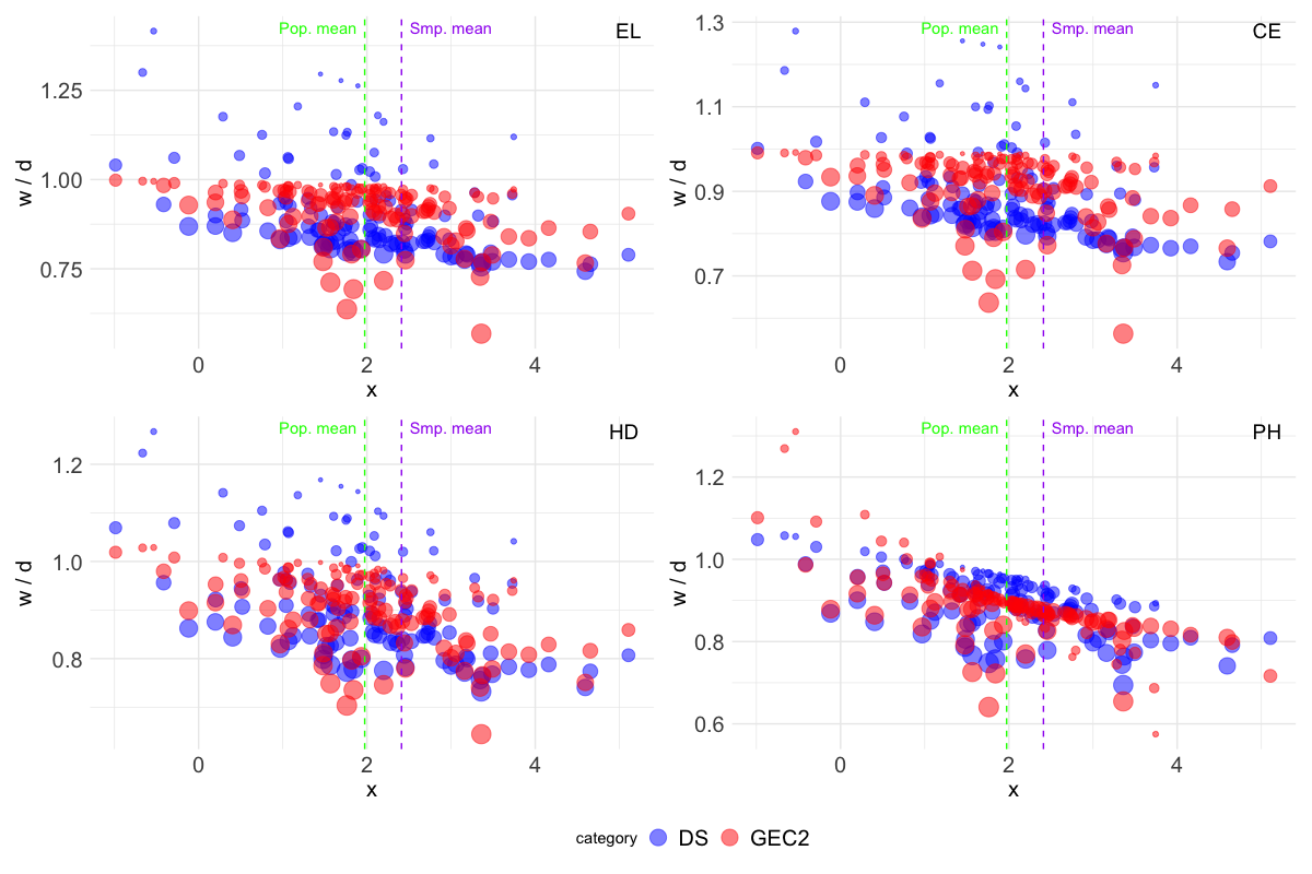
Figure 1: Scatter plots of $x_{1i}$ and ratio of calibration weights ($w_{i}/d_{i}$) using the EL, CE, HD, and PH entropies (from top left to bottom right) under Model 1 and a known $\alpha_{N}$. The same data generation setup as the simulation section is used except $N=1000$ and $x_{2i}=0$ for easy illustration. The dot size is proportional to $\log(d_{i})$.

8 Real data analysis

We present an application of the proposed method using data from a proprietary pesticide usage survey collected from GfK Kynetec in 2020. Keyetec is a private company that specializes in agricultural information systems that involve data collection from farmers in the United States. One of the main goals of this survey is to estimate the total amount ($) spent by farm operations on pesticides in each state of the United States.

The survey was carried out by stratified sampling; the population was stratified by three factors: 50 states, 60 crops, and the size of a farm (integers from 1 to 7). Since larger farms tend to use greater amounts of pesticides, the sampling design assigned a greater proportion of the sample to larger farms within each stratum to reduce variance. See Thelin and Stone, (2013) for further details on the survey design.

For each farm $i$, the study variable $y_{i}$ is the dollar amount spent on the pesticide, including the herbicide, insecticide, and fungicide produced by the five largest agrochemical companies: BASF, Bayer, Corteva Agriscience, FMC, and Syngenta. The auxiliary variables $\bm{x}_{i}$ are the harvested areas(in acres) for each crop in each multi-county area, referred to as the Crop Reporting District(CRD). Total acres harvested for each crop-by-CRD combination are available from the USDA Census of Agriculture. Throughout the United States, there were more than 20,000 samples with more than 1,000 strata. We only report the results for four states for brevity.

For estimation, we compared the Horvitz-Thompson estimator (HT), generalized regression estimator (Reg) in (2.4), pseudo-empirical estimator (PEL) in (3.9), and the proposed generalized entropy calibration estimator using empirical likelihood (EL), cross-entropy (CE), and Hellinger distance (HD) with $\hat{K}(\alpha)=(\hat{\alpha}_{\rm HT}+1)\log(\alpha+1)$, denoted as GEC2 in the previous section. Since the design weights and the auxiliary variables are not available in each population unit, the GEC method is not applicable to our data.

Table 3 summarizes the point estimates, standard errors, and 95 % confidence intervals of the estimators. All the calibration methods converge well and produce weights even when the number of auxiliary variables is greater than 30 as in Missouri. Incorporating auxiliary variables as in Reg, PEL, EL, CE, or HD dramatically improved performance compared to the Horvitz-Thompson estimator HT. The standard error of the proposed entropy calibration estimators using EL or CE was the smallest for all states reported. Although the entropy calibration estimators produce similar point estimates and standard errors as Reg or PEL estimators in Iowa and Florida, the difference between the estimators was significant in Missouri and Mississippi.

$(N,n,p)$	IA: (124947, 1197, 30)			MO: (85384, 677, 38)
Method	Est	SE	CI	Est	SE	CI
HT	667.03	18.68	(630.42, 703.63)	353.55	18.55	(317.19, 389.90)
Reg	660.27	10.59	(639.51, 681.03)	327.77	10.71	(306.79, 348.75)
PEL	660.91	10.59	(640.15, 681.67)	335.61	10.71	(314.63, 356.60)
EL	659.54	10.47	(639.02, 680.07)	327.52	10.64	(306.67, 348.36)
CE	659.51	10.47	(638.98, 680.03)	327.47	10.64	(306.62, 348.31)
HD	660.93	10.50	(640.35, 681.50)	327.78	10.66	(306.88, 348.67)

$(N,n,p)$	FL: (14573, 152, 13)			MS: (17072, 160, 19)
Method	Est	SE	CI	Est	SE	CI
HT	84.42	14.10	(56.79, 112.05)	114.01	9.79	(94.81, 133.20)
Reg	55.92	6.90	(42.40, 69.44)	119.15	5.99	(107.42, 130.89)
PEL	53.59	6.90	(40.07, 67.11)	115.96	5.99	(104.22, 127.69)
EL	54.63	6.80	(41.31, 67.95)	112.87	5.93	(101.26, 124.49)
CE	54.72	6.80	(41.40, 68.05)	112.82	5.93	(101.21, 124.44)
HD	54.39	6.80	(41.06, 67.71)	115.24	5.94	(103.59, 126.89)

Table 3: Point estimate (Est), standard error (SE), and confidence intervals (CI) of pesticide sales ($\times 10^{6}\$$) in the four states, Iowa(IA), Missouri(MO), Florida(FL), and Mississippi(MS), where $(N,n,p)$ stands for the number of farms, the number of samples, and the dimension of the auxiliary variable $\bm{x}_{i}$ in a state, respectively.

9 Concluding remarks

In this paper, we have introduced a novel approach that integrates generalized entropy with a debiasing constraint, culminating in an estimator that is both efficient and design-consistent. The proposed method ensures the stability of the calibration weights, even in the challenging situations of an informative sampling design or in the presence of disproportionately large design weights. Even when complete design information is not available throughout the population, the proposed calibration method can be developed using the adjusted generalized entropy.

Although the optimal entropy function using cross-entropy discussed in Section 5 is design-optimal under the same set of balancing functions, it may not lead to the most efficient calibration estimation for different balancing functions as we have seen in the simulation study. Choosing the best entropy function and the augmentation term $\hat{K}$ would be an interesting research problem.

A possible extension may include applying the generalized entropy for a soft calibration using the $L_{2}$ norm (Guggemos and Tillé,, 2010) or the $L_{1}$ norm (McConville et al.,, 2017; Wang and Zubizarreta,, 2020). Once the debiasing constraint is satisfied, the other benchmarking constraints can be relaxed to handle high-dimensional auxiliary variables. The new framework for debiasing calibration using generalized entropy can also be applied to missing data analysis and causal inference. Further developments in this direction will be presented elsewhere.

In addition, an R package implementing the proposed debiasing calibration weighting is under development and will be available on CRAN when it is ready.

References

- Athey et al., (2018) Athey, S., Imbens, G. W., and Wager, S. (2018). Approximate residual balancing: debiased inference of average treatment effects in high dimensions. Journal of the Royal Statistical Society: Series B, 80(4):597–623.
- Berger and Torres, (2016) Berger, Y. G. and Torres, O. D. L. R. (2016). Empirical likelihood confidence intervals for complex sampling designs. Journal of the Royal Statistical Society Series B: Statistical Methodology, 78(2):319–341.
- Breidt et al., (2005) Breidt, F. J., Claeskens, G., and Opsomer, J. D. (2005). Model-assisted estimation for complex surveys using penalised splines. Biometrika, 92(4):831–846.
- Breidt and Opsomer, (2000) Breidt, F. J. and Opsomer, J. D. (2000). Local polynomial regression estimators in survey sampling. Annals of Statistics, 28(4):1026–1053.
- Breidt and Opsomer, (2017) Breidt, F. J. and Opsomer, J. D. (2017). Model-assisted survey estimation with modern prediction techniques. Statistical Science, 32(2):190–205.
- Chen and Sitter, (1999) Chen, J. and Sitter, R. R. (1999). A pseudo empirical likelihood approach to the effective use of auxiliary information in complex surveys. Statistica Sinica, 9(2):385–406.
- Dagdoug et al., (2023) Dagdoug, M., Goga, C., and Haziza, D. (2023). Model-assisted estimation through random forests in finite population sampling. Journal of the American Statistical Association, 118:1234–1251.
- Devaud and Tillé, (2019) Devaud, D. and Tillé, Y. (2019). Deville and Särndal’s calibration: revisiting a 25-years-old successful optimization problem (with discussion). Test, 28:1033–1065.
- Dever and Valliant, (2016) Dever, J. A. and Valliant, R. (2016). General regression estimation adjusted for undercoverage and estimated control totals. Journal of Survey Statistics and Methodology, 4:289–318.