Survival of Gas in Subhalos and Its Impact on the 21 cm Forest Signals: Insights from Hydrodynamic Simulations

Abstract

Understanding the survival of gas within subhalos under various astrophysical processes is crucial for elucidating cosmic structure formation and evolution. We study the resilience of gas in subhalos, focusing on the impact of tidal and ram pressure stripping through hydrodynamic simulations. Our results uncover significant gas stripping primarily driven by ram pressure effects, which also profoundly influence the gas distribution within these subhalos. Notably, despite their vulnerability to ram pressure effects, the low-mass subhalos can play a pivotal role in influencing the observable characteristics of cosmic structures due to their large abundance.

Specifically, we explore the application of our findings to the 21 cm forest, showing how the survival dynamics of gas in subhalos can modulate the 21 cm optical depth, a key probe for detecting minihalos in the pre-reionization era. Our previous study demonstrated that the 21-cm optical depth can be enhanced by the subhalos, but the effects of tidal and ram pressure stripping on the subhalo abundance have not been fully considered. In this work, we further investigate the contribution of subhalos to the 21 cm optical depth with hydrodynamics simulations, particularly highlighting the trajectories and fates of subhalos within mass ranges of $10^{4-6}M_{\odot}h^{-1}$ in a host halo of $10^{7}M_{\odot}h^{-1}$. Despite their susceptibility to ram pressure stripping, the contribution of abundant low-mass subhalos to the 21-cm optical depth is more significant than that of their massive counterparts primarily due to their greater abundance. We find that the 21-cm optical depth can be increased by a factor of approximately two due to the abundant low-mass subhalos. However, this enhancement is about three times lower than previously estimated in our earlier study, a discrepancy attributed to the effects of ram pressure stripping. Our work provides critical insights into the gas dynamics within subhalos in the early Universe, highlighting their resilience against environmental stripping effects, and their impact on observable 21-cm signals.

I Introduction

In the standard $\Lambda$CDM model, the structure formation proceeds according to the bottom-up fashion, and minihalos whose CDM mass ranges from $\sim 10^{4}M_{\odot}$ to $\sim 10^{7}M_{\odot}$ are expected to collapse before the reionization epoch. Therefore, discovering such small-scale objects is important to confirm the CDM cosmology. However, minihalos have not been observed yet, even with the latest telescopes, because their mass range is too small to detect.

Since minihalos are expected to contain abundant HI gas, observing HI is one way to detect the minihalos. Unfortunately, the well-known HI Lyman-$\alpha$ forest is not available for this purpose because its cross-section is too large, and the absorption feature is easily damped by HI gas in the intergalactic medium (IGM). An alternative absorption signal from HI gas is the hyperfine transition, the so-called 21 cm line, whose cross-section is very small compared to Lyman-$\alpha$. Though the 21 cm emission from minihalos could be strong [1], it is difficult to spatially resolve minihalos [2, 3]. On the other hand, observing the 21 cm absorption feature is still a promising approach to detect minihalos. Previous theoretical studies have shown that the 21 cm optical depth of minihalos is $\sim 0.01-0.1$ [4, 5], hence the Square Kilometre Array (SKA) would detect the signal if there are radio loud background sources which are brighter than $\sim 10$ mJy.

According to the bottom-up scenario, minihalos universally contain the internal dense structures so-called subhalos. Recently, Kadota et al. (2023) [6] (hereafter K23) studied the impact of subhalos to the 21 cm optical depth. The virial temperature $T_{\mathrm{vir}}$ is related to the halo mass as $T_{\mathrm{vir}}\propto M^{2/3}$. Hence, the subhalos have lower temperatures than the host halo. For the sake of the fact that 21 cm optical depth is roughly proportional to the inverse of the spin temperature [7, 8, 9, 10], which is close to the gas kinetic temperature in a halo, the subhalos likely enhance the 21 cm optical depth. In K23, we analytically estimated the 21 cm optical depth of subhalos in a host halo and concluded that the subhalos can boost the total 21 optical depth by a factor of 4. However, some significant effects were not taken into account in K23. For instance, when subhalos move in a host halo, they always suffer from tidal and ram pressure forces. Subhalos are consequently expected to lose their gas mass during their motion, reducing their optical depth. It is also expected that the dynamical friction effectively works in a gas-rich system, and subhalos could quickly fall towards the center of the host halo, where the tidal and ram pressure forces strongly work. In addition to these dynamical phenomena, there are thermal aspects to consider, including compressional heating. In K23, the halos are assumed to be in the isothermal state at all times. But, in the realistic case, the compression would heat the subhalos and decrease their optical depth.

In order to obtain a more accurate estimation of the subhalo contribution to the 21 cm forest signal, it is necessary to take into account these physical effects. However, these effects are difficult to consider analytically. Therefore, in this study, we conduct hydrodynamics simulations to evaluate the 21 cm optical depth while accounting for these effects. To compute the 21 cm optical depth, taking into account subhalos, we take two steps. In the first step, we perform hydrodynamic simulations in which a subhalo of various masses moves within a host halo. Using simulation data, we evaluate the time evolution and spatial distribution of 21 cm optical depth originating from a moving subhalo. Then, in the second step, we calculate the total 21 cm optical depth with subhalos following a subhalo mass function by performing the subhalo mass function weighted integration of the optical depths of subhalos derived from the simulations. Hereafter, the subscript $\mathrm{h}$ denotes the physical value of a host halo, and $\mathrm{s}$ does that of subhalos.

Throughout this study, we assume the $\Lambda$CDM model with cosmological parameters: $h=0.674$, $\Omega_{m}=0.315$, $\Omega_{b}h^{2}=0.02237$, $\Omega_{\Lambda}=0.685$ based on Plank 2018 result [11]. Our paper is organized as follows. In Section II, we explain the setup of our simulations and show the simulation results. In Section III, we describe how to compute and estimate the 21 cm optical depth of the subhalos along the line of sight (LOS) inside the minihalo using our simulation data, and present our results and compare them to those of K23. Finally, Sections IV and V are respectively devoted to the discussion and summary.

II Hydrodynamics simulations

As mentioned in the introduction, to evaluate the 21 cm optical depth of a minihalo, we need to know the dynamical and thermal evolution of subhalos as they move inside the host halo. For this purpose, we conduct numerical simulations in which dark matter (DM) and baryon dynamics are solved simultaneously. We utilize a hydrodynamics simulation code START, [12] which employs smoothed particle hydrodynamics (SPH) method. The halo masses we consider in this work are less than $10^{7}M_{\odot}$ where atomic cooling hardly works. Therefore we ignore the radiative cooling for simplicity, and the baryon is assumed to evolve adiabatically.

II.1 Simulation Setup

We employ the same initial condition used in K23 to directly compare results (Appendix A describes the initial conditions concretely). A host halo and a subhalo have the same density profile except for the region outside the virial radius. We first place a DM halo with the Navarro, Frenk & White (NFW) profile [13, 14] at $z=10$ for which the concentration parameter is taken from the fitting formula of [15]. Then, we distribute the baryon component to obey the isothermal hydrostatic equilibrium with $T_{\rm gas}=T_{\rm vir}$. With this setup, the halo artificially expands due to the vacuum boundary condition. Therefore, we also distribute the IGM particles surrounding the host halo to moderate the artificial expansion of the halo. As for the IGM particles, we extrapolate the gas density profile up to $2R_{\mathrm{vir},\mathrm{h}}$ and set $T=2.18\rm K$ which corresponds to the temperature of adiabatically cooled gas at $z=10$. The enclosed gas mass fraction is set to be $f_{\mathrm{b}}=\Omega_{\mathrm{b}}/\Omega_{\mathrm{m}}=0.156$. In this work, the host halo mass $M_{\mathrm{h}}$ is fixed to be $10^{7}M_{\odot}/h$, and subhalo masses $m_{\mathrm{s}}$ are $10^{6}$, $5\times 10^{5}$, $10^{5}$, $5\times 10^{4}$, $3\times 10^{4}$, and $10^{4}M_{\odot}/h$ in each run. We set the gas-particle mass to $10f_{\mathrm{b}}M_{\odot}/h$ and the DM particle mass to $10(1-f_{\mathrm{b}})M_{\odot}/h$ so that the mass resolution is identical in all runs. The simulations are performed for about 4 times a characteristic dynamical time scale ($\sqrt{1/G\bar{\rho}_{\mathrm{h}}}$), which corresponds to about 40 % of the age of the Universe.

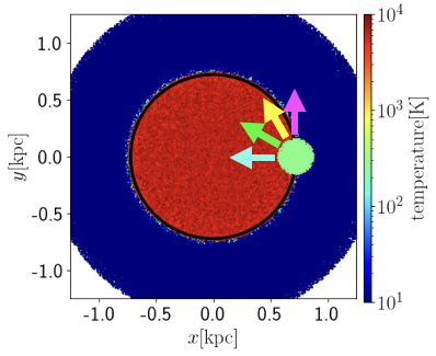
Figure 1: An initial state of a minihalo in the equatorial ($x-y)$ plane. The color indicates the gas temperature. The region where the temperature is higher than $\sim 10^{3}\rm K$ corresponds to the minihalo with the size of $R_{\mathrm{vir},\mathrm{h}}$, and the outer low-temperature region is the IGM region. A subhalo is initially at the position of ($x$, $y$, $z$) = ($R_{\mathrm{vir},\mathrm{h}}$, 0, 0) and has the initial velocity of $|\sqrt{GM_{\mathrm{vir},\mathrm{h}}}/R_{\mathrm{vir},\mathrm{h}}|$ with different entry angles of 0 (the magenta arrow), 30 (yellow), 60 (yellow-green), and 90 (cyan) degrees.

We show an initial state of the simulation in Fig. 1. In all runs, a subhalo with $m_{\mathrm{s}}$ starts to move from the position ($x$, $y$, $z$) = ($R_{\mathrm{vir},\mathrm{h}}$, 0, 0) (see Fig. 1). We consider four entry angles, $\theta_{\rm ini}$ of $0^{\circ}$ (circular motion), $30^{\circ}$, $60^{\circ}$, and $90^{\circ}$ (radial motion). It is expected that the potential energy and the kinetic energy almost balance with each other when subhalos merge with the host halo. Therefore, we fix the magnitude of the initial velocity to be the Kepler velocity $v_{\rm ini}=\sqrt{GM_{\mathrm{h}}/R_{\mathrm{vir},\mathrm{h}}}=9.39\rm km/s$, and assume that the initial velocity is independent of the entry angle for simplicity.

II.2 Evolution of Subhalos

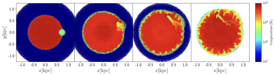
Figure 2: Two-dimensional color maps showing the time evolution of the gas temperature. Snapshots every 47.2 Myr from the initial time are shown from left to right. The top, middle, and bottom rows respectively represent results with the parameter set of $(m_{\mathrm{s}},\theta_{\rm ini})=(10^{5}M_{\odot}/h,0^{\circ})$, $(10^{5}M_{\odot}/h,30^{\circ})$, and $(10^{4}M_{\odot}/h,0^{\circ})$.

We first show the evolution of subhalos in Fig. 2. From left to right, each panel shows the snapshot at $t\approx 0$, 47.2 $\mathrm{Myr}$, 94.4 $\mathrm{Myr}$ and 142 $\mathrm{Myr}$, respectively. In the figures, the color represents gas temperature. The top row shows the result of the parameter set of $(m_{\mathrm{s}},\theta_{\rm ini})=(10^{5}M_{\odot}/h,0^{\circ})$. In this case, the subhalo is initially heated up to $1.5T_{\mathrm{vir}}$ by the compressional heating. After that, the gas in the subhalo is considerably stripped off during $\sim 100\mathrm{Myr}$. The left panel of Fig. 3 quantitatively displays the time evolution of the gas and DM mass fractions, defined as the fraction of the bound gas and DM mass to each initial mass. For this analysis, we select particles whose total energy is negative as ”bound” particles. By $\sim 100\mathrm{Myr}$, $20\%$ of the DM is stripped off from the subhalo. On the other hand, the gas mass stripping is stronger than the DM mass stripping, and only $10\%$ of the initial gas remains. Such a difference is caused by the forces they receive. In fact, the DM component is only affected by the tidal force, while the gas component is affected by both the tidal force and the ram pressure. Therefore, the ram pressure effect mainly causes the gas mass stripping. To gain a better understanding of ram pressure stripping, the right panel in Fig. 3 shows the time evolution of the ratio between the ram pressure ($P_{\mathrm{ram}}$) and the maximum gravitational restoring force per unit area ($f_{\mathrm{g}}$) [16] expressed as

$$P_{\mathrm{ram}}/f_{\mathrm{g}}=\frac{\rho_{\mathrm{gas},\mathrm{h}}v_{\mathrm{orb}}^{2}}{\gamma Gm_{\mathrm{s}}(R_{\mathrm{s}})\rho_{\mathrm{gas},\mathrm{s}}(R_{\mathrm{s}})/R_{\mathrm{s}}}~{},$$ (1)

where $\gamma$ is a parameter depending on the density profile. We apply $\gamma=\pi/2$ in this study because the singular isothermal sphere can approximate the gas density profile (appendix B). Eq. (1) indicates that $f_{\rm g}$ is initially proportional to $m_{\rm s}^{2/3}$ and less massive halos are more susceptible to the ram pressure than massive subhalos. Figure 3 shows that the ram pressure considerably overcomes the gravitational restoring force per area at the initial phase, resulting in significant gas mass loss. Since the subhalo density approximately follows the singular isothermal profile, the gravitational restoring force is stronger at the inner part of the subhalo as $f_{\rm g}\propto\rho^{2}R_{\mathrm{s}}^{2}\propto R_{\mathrm{s}}^{-2}$. Therefore, as the outer side is stripped by ram pressure stripping, $f_{\rm g}$ eventually approaches $P_{\rm ram}$, mitigating mass loss in later stages. This is the common trend in all simulation runs.

The middle row of Fig. 2 shows the evolution of $(m_{\mathrm{s}},\theta_{\rm ini})=(10^{5}M_{\odot}/h,30^{\circ})$. Since the subhalo passes through the inner high-density region, the ram pressure strongly works and the gas stripping is more prominent than the case of $(m_{\mathrm{s}},\theta_{\rm ini})=(10^{5}M_{\odot}/h,0^{\circ})$ (the top row). Finally, the bottom row of Fig. 2 represents the case of a lower subhalo mass of $m_{\mathrm{s}}=10^{4}M_{\odot}/h$. In this case, ram pressure significantly affects the subhalo, leading to a drastic stripping of gas due to a weak gravitational restoring force.

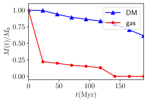
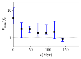
Figure 3: Both panels are the results of $(m_{\mathrm{s}},\theta_{\rm ini})=(10^{5}M_{\odot}/h,0^{\circ})$. Left: The mass fractions of gas (red circles) and DM (blue triangles) to the initial gas/DM mass ($M_{0}$) of the subhalo as a function of time. After $90$ % of the initial mass is removed, the halo is considered a disrupted halo in this analysis. Right: The ratio of the ram pressure $P_{\mathrm{ram}}$ to the maximum gravitational restoring force per unit area $f_{\mathrm{g}}$ as a function of time [16]. The $10$ % of the outermost bounded particles are used to evaluate $f_{g}$ for this analysis, while all bounded particles are used when the number of the bound particles is less than $100$. The squares represent the median values, and the error bars are drawn from the maximum and minimum values.

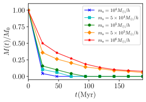
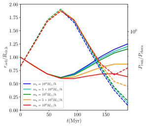
Figure 4: Left: The time evolution of the gas mass fractions of subhalos with $m_{\mathrm{s}}=10^{4}M_{\odot}/h$ (crosses, blue), $5\times 10^{4}M_{\odot}/h$ (squares, cyan), $10^{5}M_{\odot}/h$ (circles, green), $5\times 10^{5}M_{\odot}/h$ (diamonds, orange), and $10^{6}M_{\odot}/h$ (stars, red). The initial entry angle is $30^{\circ}$ for all cases. Right: The time evolution of the subhalo’s orbital radius $r_{\mathrm{orb}}$ (the solid lines) and the ram pressure (the dashed lines). The orbital radius and the ram pressure are respectively normalized by the host halo virial radius and by the characteristic value of $P_{\mathrm{chara}}=\bar{\rho}_{\mathrm{halo,b}}\;v_{\mathrm{cir}}(R_{\mathrm{vir},\mathrm{h}})^{2}$, where $\bar{\rho}_{\mathrm{halo,b}}$ is the averaged baryon density of a virialized halo collapsed at $z=10$ and $v_{\mathrm{cir}}(R_{\mathrm{vir},\mathrm{h}})$ is the circular velocity at the virial radius.

The left panel of Fig. 4 summarizes the evolution of the baryon mass fractions for various subhalo masses with $\theta_{\rm ini}=30^{\circ}$. As discussed above, the balance between the ram pressure and the gravitational restoring force determines the final mass fraction. As stated above, the less massive subhalos have less gravitational restoring force per area and more susceptible to the ram pressure for a given ram pressure. Therefore, the final mass fraction tends to be smaller for the less massive subhalos. However, at a later phase of $t\gtrsim 75\mathrm{Myr}$, the mass dependence seems to be relatively weak. The evolution of the orbital radii and the resultant ram pressure of subhalos is shown in the right panel of Fig. 4 to understand the reason why the mass dependence becomes weak. Compared to less massive subhalos, massive subhalos’ orbital radii tend to be small at $t\gtrsim 75\mathrm{Myr}$ due to the dynamical friction. Consequently, the ram pressure strongly works for massive subhalos.

In conclusion, we find that the gas temperature of subhalos is initially increased by a factor of about 1.5 due to the compressional heating, and then a large amount of the gas is stripped by the ram pressure. The effect of the ram pressure is noticeable for less massive subhalos that are destroyed by $\sim 100\mathrm{Myr}$. Both the heating and the disruption would lead to a reduction in the 21 cm optical depth. Consequently, the contribution, especially by smaller subhalos, declines compared to K23. We should note that, even after most of the gas is stripped from a subhalo, the stripped gas still keeps a lower gas temperature than the host halo gas, as shown in Fig. 2. Thus, the disrupted subhalos still contribute to the total 21 cm optical, as we will show later.

III Calculating 21 cm optical depth

In this section, we estimate the optical depths originating from subhalos using the hydrodynamics simulation results. The 21 cm optical depth is calculated as

$$\tau=\frac{3h_{\mathrm{p}}c^{3}A_{10}}{32\pi k_{\mathrm{B}}\nu_{21}^{2}}\int_{-l_{\mathrm{max}}\left(\alpha_{\mathrm{h}}\right)}^{l_{\mathrm{max}}\left(\alpha_{\mathrm{h}}\right)}\mathrm{d}l\frac{n_{\mathrm{HI}}\left(R_{\mathrm{h}}\right)}{T_{\mathrm{s}}\left(R_{\mathrm{h}}\right)\sqrt{\pi}b(R_{\mathrm{h}})},$$ (2)

where $\alpha_{\mathrm{h}}$, $h_{\rm p}$, $c$, $A_{10}$, $k_{\rm B}$, and $\nu_{21}$ are the impact parameter, the Planck constant, the speed of light, the Einstein coefficient, the Boltzmann constant, and the frequency corresponding to 21 cm line, respectively. $l$ is the path along the LOS with $l=\sqrt{R_{\mathrm{h}}-\alpha_{\mathrm{h}}}$, $l_{\mathrm{max}}=\sqrt{R_{\mathrm{vir},\mathrm{h}}-\alpha_{\mathrm{h}}}$, and $b$ is the velocity dispersion $b^{2}=2k_{\mathrm{B}}T(R_{\mathrm{h}})/m_{\mathrm{p}}$. The spin temperature $T_{\rm s}$ is computed using the collisional coupling [17, 18, 19, 20].

Figure 5 shows the spatial distribution at different times of the optical depth of a minihalo containing only one subhalo with $(m_{\mathrm{s}},\theta_{\rm ini})=(10^{5}M_{\odot}/h,0^{\circ})$ along the LOS parallel to the y-axis in the equatorial plane. The horizontal axis is the distance from the center. A clear peak initially appears at $x/R_{\mathrm{vir},\mathrm{h}}=1.0$, because the subhalo gas is not stripped yet. As time passes, the peak gradually decreases due to the gas stripping and almost disappears by $t\approx 140\mathrm{Myr}$. However, as mentioned above, the stripped gas has a lower temperature than the host halo, so the subhalo slightly contributes to the total optical depth.

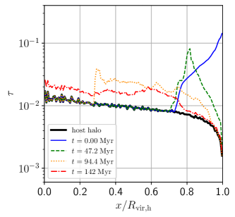
Figure 5: The optical depth along the LOS parallel to the y-axis in the equatorial plane (z = 0) for $(m_{\mathrm{s}},\theta_{\rm ini})=(10^{5}M_{\odot}/h,0^{\circ})$, which corresponds to the top row of Fig. 2. The thick black curve represents the optical depth without subhalos, while the thin curves the optical depths with a subhalo at $t=0.00~{}\mathrm{Myr}$ (solid, blue), $t=47.2~{}\mathrm{Myr}$ (dashed green), $t=94.4~{}\mathrm{Myr}$ (dotted orange), $t=142~{}\mathrm{Myr}$ (dash-dotted red). When $t=142~{}\mathrm{Myr}$, over $90$ % of the subhalo gas mass is stripped off.

Based on Fig. 5, we then evaluate the total 21 cm optical depth of subhalos which follow a subhalo mass function $\frac{\mathrm{d}n_{\mathrm{s}}}{\mathrm{d}m_{\mathrm{s}}}$. Here, we use the same subhalo mass function as used in K23 [6, 21, 22], but use a different spatial distribution of subhalos from K23 in which they assumed that the number density of subhalos obeys NFW profile or uniform distribution inside a host halo. In our simulations, the position of a subhalo depends on the elapsed time and its entry angle. Assuming subhalos randomly accrete onto the host halo, we take the time average over our total simulation time for a given impact parameter $\alpha_{\mathrm{h}}$ and get the time-averaged value $\bar{\tau}$. (The total time for our simulations is about $4\sqrt{1/G\bar{\rho}_{\mathrm{h}}}$ (4 times a characteristic dynamical time scale) as mentioned in Section II-A). Eventually, the total optical depth of subhalos for a given entry angle $\theta_{\rm ini}$ is expressed as

$$\tau_{\mathrm{s}}^{\omega}\left(\alpha_{\mathrm{h}},\theta_{\rm ini}\right)=\int_{10^{4}M_{\odot}/h}\mathrm{d}m_{\mathrm{s}}\left.\frac{\mathrm{d}n_{\mathrm{s}}}{\mathrm{d}m_{\mathrm{s}}}\left(m_{\mathrm{s}}\right)\right|_{M_{\mathrm{h}}=10^{7}M_{\odot}/h}\bar{\tau}(m_{\mathrm{s}},\alpha_{\mathrm{h}},\theta_{\rm ini}),$$ (3)

where $\alpha_{\mathrm{h}}$ is the impact parameter. Here, this $\tau_{\mathrm{s}}$ relies on the direction of LOS which is represented by the subscript $\omega(=x,y,z)$. We shall discuss this in the next paragraph. The applied subhalo mass function contains a cut-off above which the number of subhalos exponentially decrease. The lower limit of $10^{4}M_{\odot}/h$ roughly corresponds to the Jeans mass. With respect to the mass integration, we only have the discrete dataset ranging from $10^{4}M_{\odot}/h$ to $10^{6}M_{\odot}/h$. Therefore, we interpolate and extrapolate them linearly with 60 mass bins to complete the integration using SciPy.

Figure 6 shows $\tau_{\mathrm{s}}^{\omega}(\alpha_{\mathrm{h}},\theta_{\rm ini})$ for several entry angles. The left panel of Fig. 6 represents the results with the LOS parallel to the x-axis (cf. Fig. 1).

Since the subhalo initially exists at $\alpha_{\mathrm{h}}=0$ without disruption, the optical depth at $\alpha_{\mathrm{h}}\sim 0$ is very high for all entry angles. When $\theta_{\rm ini}=0^{\circ}$, the subhalo is moving in a circular orbit, and hence the gas in the subhalo is extended up to $R_{\mathrm{vir},\mathrm{h}}$. The central panel shows the case with the LOS being along the $y$-axis. Obviously, the distribution of the optical depth hardly depends on $\theta_{\rm ini}$ in this case. The high optical depth at the outer region simply comes from the subhalos at the initial stage. The optical depth at the central region is also relatively high because all subhalos inevitably pass through the $\alpha_{\mathrm{h}}\approx 0$ region. The right panel for the LOS is parallel to the $z$-axis. Similar to the case of the central panel, the optical depth in the outer region is high for all entry angles owing to the subhalos at the initial position. The subhalos with $\theta_{\rm ini}=90^{\circ}$ straightly fall towards the center, while those with $\theta_{\rm ini}=0^{\circ}$ never reach the central region. Therefore, the optical depth in the inner region depends strongly on the entry angle.

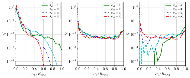
Figure 6: The time-averaged optical depth of subhalos following the subhalo mass function. The shown optical depths are averaged in a thin ring with a given impact parameter. The solid green, dashed cyan, dotted blue, and dash-dotted red curves show the results with $\theta_{\rm ini}=0^{\circ}$, $\theta_{\rm ini}=30^{\circ}$, $\theta_{\rm ini}=60^{\circ}$, and $\theta_{\rm ini}=90^{\circ}$, respectively. The left, central, and right panels, respectively, show the values along the x-, y-, and z-axes (cf. Fig. 1).

Finally, we compare our results with the analytic estimation by K23. For this purpose, we take average of $\tau_{\mathrm{s}}^{\omega}$ over three line-of-sights and four entry angles:

$$\tau_{\mathrm{ave},\mathrm{s}}(\alpha_{\mathrm{h}})=\frac{\sum_{\omega}\sum_{\theta_{\rm ini}}\tau_{\mathrm{s}}^{\omega}\left(\alpha_{\mathrm{h}},\theta_{\rm ini}\right)}{\sum_{\rm\omega}\sum_{\theta_{\rm ini}}}.$$ (4)

The denominator represents the number of the ensemble of our simulation. The profile of $\tau_{\rm ave,\mathrm{s}}$ would depend on LOS directions taken in the ensemble, and we for simplicity take the average over LOS directions parallel to x, y, and z axes in our study shown in Fig. 6. (So the denominator is $\sum_{\rm\omega}\sum_{\theta_{\rm ini}}=12$ in this study). We also quantify the subhalos’ contribution by using the boost factor, defined as the subhalo optical depth ratio to the host halo optical depth, $B\equiv\tau_{\rm ave.\mathrm{s}}/\tau_{\mathrm{h}}$ as is in K23. Figure 7 shows the optical depth of subhalos (left) and the boost factor (right). In each panel, the thick (blue) curve is our simulation result, and the thin (black) ones are results from K23 .

With respect to the outer region of $\alpha_{\mathrm{h}}/R_{\mathrm{vir},\mathrm{h}}\gtrsim 0.9$, our result shows higher optical depth than the K23 ”fiducial.” This is caused by the difference in the spatial distribution of subhalos. The NFW profile assumed in the K23 ”fiducial” model causes the number density of subhalos at this region to be smaller than our simulations. On the other hand, the distribution of subhalos in our simulations roughly corresponds to the uniform distribution because the optical depth shown here is the time-averaged value. In fact, the optical depth at $\alpha_{\mathrm{h}}/R_{\mathrm{vir},\mathrm{h}}\gtrsim 0.9$ in the simulation is almost consistent with that in the K23 ”uniform” model. In the middle region of $0.2\lesssim\alpha_{\mathrm{h}}/R_{\mathrm{vir},\mathrm{h}}<0.9$, our result is lower than the K23 ”fiducial” model because the gas mass stripping by the ram pressure works and the subhalos contribute to the optical depth modestly. Finally, with regard to the innermost region $\alpha_{\mathrm{h}}/R_{\mathrm{vir},\mathrm{h}}<0.2$, the optical depth steeply increases towards the center and eventually exceeds the K23 ”fiducial” model at $\alpha_{\mathrm{h}}\approx 0$. This behavior is essentially caused by the same reason as shown in Fig. 6. All subhalos pass through the $\alpha_{\mathrm{h}}\approx 0$ region, except for cases where LOS is parallel to the z-axis (the right panel of 6). In particular, when we chose the LOS along the x-axis (the left panel of Fig. 6), all subhalos are initially at $\alpha_{\mathrm{h}}\approx 0$ without destruction. Therefore, we notice that this profile of $\tau_{\mathrm{ave,s}}$ should be modified if we consider the ensemble average over all LOS directions.

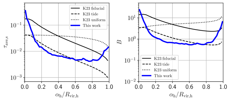
Figure 7: The subhalo optical depth (Left) and the boost factor $B$ (Right) as a function of the impact parameter normalized to the host halo virial radius at z = 10. The thick (blue) curve is our result, and the thin (black) curves are the results from K23. As for K23 results, the solid curve represents the case where the subhalos are not affected by the stripping and are distributed following the NFW profile of the host halo. The dashed curve represents the case that the outer regions $r>0.77r_{\mathrm{s},\mathrm{s}}$ of the subhalos are assumed to be stripped completely, where $r_{\mathrm{s},\mathrm{s}}$ is the subhalo’s scale radius. The dotted curve represents the case that the subhalos without mass stripping are uniformly distributed.

We emphasize that the most important value here is the optical depth averaged over the apparent area which does not depend on the choice of the LOS since the spatial distribution of $\tau_{\rm ave,\mathrm{s}}$ in each minihalo cannot be observationally resolved even with the SKA. The boost factor of a minihalo averaged over the apparent area is given by

$$B_{\mathrm{halo}}=\frac{\int^{R_{\mathrm{vir},\mathrm{h}}}_{0}2\pi\alpha B(\alpha)\mathrm{d}\alpha}{\int^{R_{\mathrm{vir},\mathrm{h}}}_{0}2\pi\alpha\mathrm{d}\alpha}.$$ (5)

where $B$ is defined below Eq. 4. We find that the boost factor derived from our simulations is $B_{\mathrm{halo,sim}}\approx 1.20$, whereas that in the K23 ”fiducial” model is $B_{\mathrm{halo,K23}}\approx 3.67$. Thus, we conclude that the hydrodynamic effects, such as the ram pressure and the compressional heating , reduce the 21 cm optical depth of subhalos to down to $\sim 1/3$ compared to the analytic estimate. It should be emphasized that subhalos in a minihalo whose mass is $10^{7}M_{\odot}/h$ can enhance the optical depth by a factor $(1+B_{\mathrm{halo}})\sim 2$, even if the hydrodynamic effects are considered.

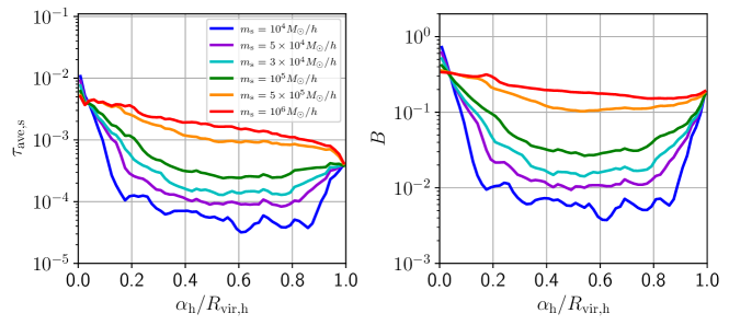
Figure 8: Left panel: the optical depths of one subhalo with $m_{\mathrm{s}}=10^{4}M_{\odot}/h$ (blue), $3\times 10^{4}M_{\odot}/h$ (purple), $5\times 10^{4}M_{\odot}/h$ (cyan), $10^{5}M_{\odot}/h$ (green), $5\times 10^{5}M_{\odot}/h$ (orange), and $10^{6}M_{\odot}/h$ (red). Right panel: the corresponding boost factors.

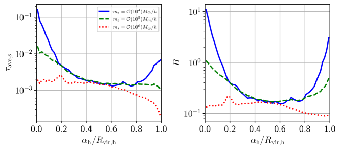
Figure 9: Left: The subhalo mass function weighted optical depths ($\tau_{\mathrm{ave}}$ in Eq. 4) for three integration regions of $10^{4}M_{\odot}/h\leq m_{\mathrm{s}}<10^{5}M_{\odot}/h$ (solid, blue), $10^{5}M_{\odot}/h\leq m_{\mathrm{s}}<10^{6}M_{\odot}/h$ (dashed, green), and $10^{6}M_{\odot}/h\leq m_{\mathrm{s}}<10^{7}M_{\odot}/h$ (dotted, red). Right: The corresponding boost factors.

In addition, we investigate which mass scale is responsible for the optical depth. Fig. 8 shows the time-averaged optical depth of one subhalo with various masses (left) and the corresponding boost factor (right). One can observe that the optical depth increases with the mass of subhalos. As stated in Section I, the optical depth of a low-mass halo is higher than that of a massive halo, as long as the subhalo is not affected by the tidal force and ram pressure. However, as shown in Fig. 4, low-mass subhalos are more sensitive to the ram pressure than massive ones . When the ram pressure just starts to work, the strong gas stripping for a less massive subhalo compensates for the high optical depth of the subhalo. As a result, the optical depth is almost independent of the subhalo mass at $\alpha/R_{\mathrm{vir},\mathrm{h}}\sim 1$. Less massive subhalos considerably lose their gas component as time passes, and the optical depth is smaller than massive subhalos in $0.2\lesssim\alpha/R_{\mathrm{vir},\mathrm{h}}\lesssim 0.9$ region.

The left panel of Fig.9 shows the subhalo mass function weighted optical depth for three different integration ranges of $10^{4}M_{\odot}/h\leq m_{\mathrm{s}}<10^{5}M_{\odot}/h$, $10^{5}M_{\odot}/h\leq m_{\mathrm{s}}<10^{6}M_{\odot}/h$, and $10^{6}M_{\odot}/h\leq m_{\mathrm{s}}<10^{7}M_{\odot}/h$. Interestingly, considering the subhalo mass function, the total contribution from more abundant low-mass subhalos is more dominant than that from less abundant high-mass subhalos owing to the strong mass dependence of the adapted subhalo mass function. In summary, although the contribution to the optical depth from a low-mass subhalo is smaller than that from a massive subhalo due to the former’s vulnerability to gas stripping, the cumulative contribution from low-mass subhalos becomes dominant overall because of their greater abundance.

IV Discussion

In this section, we discuss some points that may affect our results. One may claim that the gas mass stripping can be caused by the Kelvin-Helmholtz (KH) and Rayleigh-Taylor (RT) instabilities. If this is the case, the standard SPH method is known to overestimate the effects. According to previous studies [16, 23], the KH time-scale can be estimated by,

$$t_{\mathrm{KH}}=2.19\times 10^{9}\left(\frac{F}{0.1}\right)\left(\frac{m_{\mathrm{s}}}{10^{9}M_{\odot}}\right)^{1/7}\left(\frac{n_{\mathrm{h}}}{10^{-4}\;\mathrm{cm}^{-3}}\right)^{-1}\left(\frac{v_{\mathrm{orb}}}{10^{3}\;\mathrm{km/s}}\right)^{-1}\mathrm{yr},$$ (6)

where $F$ is the baryon fraction of the halos, $m_{\mathrm{s}}$ is the subhalo mass, $n_{\mathrm{h}}$ is the number of the hydrogen atoms in the host halo, and $v_{\mathrm{orb}}$ is the velocity of the subhalo with respect to the host halo. In our simulations, the estimated KH time-scale is $t_{\mathrm{KH}}\sim 213~{}\mathrm{Myr}$, which is longer than the timescale of the gas stripping of $\sim 100~{}\mathrm{Myr}$. Therefore, we conclude that the gas stripping is not mainly caused by the instabilities, and our standard SPH method would not overestimate the mass loss in our simulations.

We employed a somewhat simplified model for halos in this study. First, we assumed the collapse redshift of $z=10$ for the host halo and the subhalos. However, according to the bottom-up scenario, the subhalos should collapse before the formation time of the host halo. In this case, the subhalos have higher gas density and are more resistant to gas stripping , and this causes the optical depth of the subhalos to be larger. For example, as for $z=15$, the subhalo gas particles are bounded about 1.5 - 2.0 times longer than $z=10$ by our simulation. On the other hand, as showed by [24], the halos at higher redshift have less optical depth roughly because of their higher virial temperature at higher redshift leading to reducing their own optical depth. Hence, the optical depth of the subhalos is expected not to be influenced so much by offsetting these effects even considering the clumpiness of the subhalos, or can be larger to some extent than our results if the survivability works effectively.

As for the temperature distribution, we assumed that subhalos initially have uniform distribution with their virial temperature. However, in the case of adiabatic collapse, halos usually have higher temperatures in the central core region than in the outer region. The temperature distribution is more complicated with the cooling effect, which is completely neglected in our simulations. Molecular hydrogen cooling is known to be effective in a halo whose mass is greater than about $10^{5}M_{\odot}/h$. Therefore, in more realistic cases, the temperature distribution in a halo would not be uniform and would be lower than our assumption. We will investigate how the optical depth changes if these complicated factors are considered in future work.

V Summary

In this study, we first conducted hydrodynamics simulations to explore how the hydrodynamic effects, such as the ram pressure and the compressional heating, affect the evolution of subhalos in a host minihalo. We find that the subhalos are heated by the compressional heating at the earlier phase and lose a large amount of the gas component due to the ram pressure. The effects of the ram pressure are significant for less massive subhalos: in the case of $M_{\mathrm{s}}=10^{5}M_{\odot}/h$, 90% of the gas is stripped off during approximately $100$Myr.

We then used the subhalo mass function to estimate the total contribution of subhalos to the 21 cm optical depth. Upon comparing our findings with the analytic study conducted by K23, we found that the optical depth boost caused by subhalos is reduced by hydrodynamic effects to approximately one-third of its original value. However, despite the reduction, subhalos can still double the optical depth of the host halo. We also find that low-mass subhalos are responsible for the optical depth due to their rich abundance, even though the lower-mass subhalos are more vulnerable to the gas stripping by the ram pressure.

Appendix A Gas and DM density profiles

Here we introduce the properties of halos in our simulations that are the same as K23. The density profile of a DM halo is set to be the NFW profile [13, 14],

$$\rho_{\mathrm{NFW}}(r)=\frac{\rho_{0}}{\frac{r}{r_{\mathrm{s}}}\left(1+\frac{r}{r_{\mathrm{s}}}\right)^{2}},$$ (7)

where $\rho_{0}$ is

$$\rho_{0}=\frac{M_{\mathrm{DM}}\;c^{3}}{4\pi R_{\mathrm{vir}}^{3}f(c)}$$ (8)

with $f(x)=\ln{(1+x)}-x/(1+x)$, $r_{\mathrm{s}}$ is the scale radius, and $c\equiv R_{\mathrm{vir}}/r_{\mathrm{s}}$ is the concentration parameter. $R_{\mathrm{vir}}$ refers to the virial radius [7],

$$R_{\mathrm{vir}}=0.784\left(\frac{M}{10^{8}h^{-1}M_{\odot}}\right)^{1/3}\left[\frac{\Omega_{m}}{\Omega_{m}^{z}}\frac{\Delta_{c}}{18\pi^{2}}\right]^{-1/3}\left(\frac{1+z}{10}\right)^{-1}h^{-1}\;\;\mathrm{kpc}.$$ (9)

Here, $\Delta_{c}=18\pi^{2}+82d-39d^{2}$ is the over density of the virialized halo collapsing at the redshift $z$ with $d=\Omega_{\mathrm{m}}^{z}-1$ and $\Omega_{m}^{z}=\Omega_{m}(1+z)^{3}/(\Omega_{m}(1+z)^{3}+\Omega_{\Lambda})$.

As for the gas density profiles $\rho_{\mathrm{g}}(r)$, it is assumed that the gas is isothermal with $T_{\mathrm{vir}}$ and in the hydrostatic equilibrium [7, 25, 9, 26],

$$\ln{\rho_{\mathrm{g}}(r)}=\ln{\rho_{g0}}-\frac{\mu m_{\mathrm{p}}}{2k_{\mathrm{B}}T_{\mathrm{vir}}}\left[v_{\mathrm{esc}}^{2}(0)-v_{\mathrm{esc}}^{2}(r)\right],$$ (10)

where

$$v^{2}_{\mathrm{esc}}(r)=2\int^{\infty}_{r}\frac{GM(r^{\prime})}{r^{\prime 2}}dr^{\prime}=2V_{\mathrm{c}}^{2}\frac{f(cx)+cx/(1+cx)}{xf(c)},$$ (11)

$$V_{c}=\sqrt{\frac{GM}{R_{\mathrm{vir}}}}=23.4\left(\frac{M}{10^{8}h^{-1}M_{\odot}}\right)^{1/3}\left[\frac{\Omega_{m}}{\Omega_{m}^{z}}\frac{\Delta_{c}}{18\pi^{2}}\right]^{1/6}\left(\frac{1+z}{10}\right)^{1/2}\;\;\mathrm{km/s},$$ (12)

$$\rho_{g0}(z)=\frac{(\Delta_{c}/3)c^{3}e^{A}}{\int_{0}^{c}(1+t)^{A/t}t^{2}dt}\left(\frac{\Omega_{b}}{\Omega_{m}}\right)\Omega_{m}^{z}\rho_{\mathrm{crit}}(z),$$ (13)

and

$$T_{\mathrm{vir}}=1.98\times 10^{4}\left(\frac{\mu}{0.6}\right)\left(\frac{M}{10^{8}h^{-1}M_{\odot}}\right)^{2/3}\left[\frac{\Omega_{m}}{\Omega_{m}^{z}}\frac{\Delta_{c}}{18\pi^{2}}\right]^{1/3}\left(\frac{1+z}{10}\right)\;\;\mathrm{K}.$$ (14)

These equations (11), (12), (13), (14) refer to the square of the escape velocity, circular velocity, the central gas density and the virial temperature respectively.

Appendix B the approximation of the gas density distribution

The gas density profile, introduced Eq.(10) in this study, is approximated in a manner similar to the isothermal $\beta$ model as follows [25],

$$\rho_{\mathrm{g}}(r)=\frac{\rho_{\mathrm{g0}}A(b)}{\left[1+(r/r_{\mathrm{eff}})^{2}\right]^{3\beta_{\mathrm{eff}}/2}},$$ (15)

where $b=4c/27f(c)$, $A(b)=-0.178b+0.982$, $r_{\mathrm{eff}}=0.22r_{\mathrm{s}}$, and $\beta_{\mathrm{eff}}=0.9b$. Then we can approximately regard the gas density profile in our simulations as the singular isothermal profile, $\rho_{\mathrm{g}}(r)\propto r^{-2}$, so that we can adopt $\gamma=\pi/2$ in Eq. (1) and larger size subhalos have the larger maximum gravitational restoring force per unit area.

References

- Iliev et al. [2002] I. T. Iliev, P. R. Shapiro, A. Ferrara, and H. Martel, On the Direct Detectability of the Cosmic Dark Ages: 21 Centimeter Emission from Minihalos, ApJL 572, L123 (2002), arXiv:astro-ph/0202410 [astro-ph] .
- Yajima and Li [2014] H. Yajima and Y. Li, Distinctive 21-cm structures of the first stars, galaxies and quasars, MNRAS 445, 3674 (2014), arXiv:1308.0381 [astro-ph.CO] .
- Tanaka et al. [2018] T. Tanaka, K. Hasegawa, H. Yajima, M. I. N. Kobayashi, and N. Sugiyama, Stellar mass dependence of the 21-cm signal around the first star and its impact on the global signal, MNRAS 480, 1925 (2018), arXiv:1805.07947 [astro-ph.GA] .
- Shimabukuro et al. [2020a] H. Shimabukuro, K. Ichiki, and K. Kadota, 21 cm forest probes on axion dark matter in postinflationary Peccei-Quinn symmetry breaking scenarios, Phys. Rev. D 102, 023522 (2020a), arXiv:2005.05589 [astro-ph.CO] .
- Shimabukuro et al. [2020b] H. Shimabukuro, K. Ichiki, and K. Kadota, Constraining the nature of ultra light dark matter particles with the 21 cm forest, Phys. Rev. D 101, 043516 (2020b), arXiv:1910.06011 [astro-ph.CO] .
- Kadota et al. [2023] K. Kadota, P. Villanueva-Domingo, K. Ichiki, K. Hasegawa, and G. Naruse, Boosting the 21 cm forest signals by the clumpy substructures, JCAP 2023, 017 (2023), arXiv:2209.01305 [astro-ph.CO] .
- Barkana and Loeb [2001] R. Barkana and A. Loeb, In the beginning: the first sources of light and the reionization of the universe, Phys.Rep. 349, 125 (2001), arXiv:astro-ph/0010468 [astro-ph] .
- Furlanetto and Loeb [2002] S. R. Furlanetto and A. Loeb, The 21 Centimeter Forest: Radio Absorption Spectra as Probes of Minihalos before Reionization, Astrophys. J. 579, 1 (2002), arXiv:astro-ph/0206308 [astro-ph] .
- Xu et al. [2011] Y. Xu, A. Ferrara, and X. Chen, The earliest galaxies seen in 21 cm line absorption, MNRAS 410, 2025 (2011), arXiv:1009.1149 [astro-ph.CO] .
- Meiksin [2011] A. Meiksin, The micro-structure of the intergalactic medium - I. The 21 cm signature from dynamical minihaloes, MNRAS 417, 1480 (2011), arXiv:1102.1362 [astro-ph.CO] .
- Planck Collaboration et al. [2020] Planck Collaboration, N. Aghanim, Y. Akrami, M. Ashdown, J. Aumont, C. Baccigalupi, M. Ballardini, A. J. Banday, R. B. Barreiro, N. Bartolo, S. Basak, R. Battye, K. Benabed, J. P. Bernard, M. Bersanelli, P. Bielewicz, J. J. Bock, J. R. Bond, J. Borrill, F. R. Bouchet, F. Boulanger, M. Bucher, C. Burigana, R. C. Butler, E. Calabrese, J. F. Cardoso, J. Carron, A. Challinor, H. C. Chiang, J. Chluba, L. P. L. Colombo, C. Combet, D. Contreras, B. P. Crill, F. Cuttaia, P. de Bernardis, G. de Zotti, J. Delabrouille, J. M. Delouis, E. Di Valentino, J. M. Diego, O. Doré, M. Douspis, A. Ducout, X. Dupac, S. Dusini, G. Efstathiou, F. Elsner, T. A. Enßlin, H. K. Eriksen, Y. Fantaye, M. Farhang, J. Fergusson, R. Fernandez-Cobos, F. Finelli, F. Forastieri, M. Frailis, A. A. Fraisse, E. Franceschi, A. Frolov, S. Galeotta, S. Galli, K. Ganga, R. T. Génova-Santos, M. Gerbino, T. Ghosh, J. González-Nuevo, K. M. Górski, S. Gratton, A. Gruppuso, J. E. Gudmundsson, J. Hamann, W. Handley, F. K. Hansen, D. Herranz, S. R. Hildebrandt, E. Hivon, Z. Huang, A. H. Jaffe, W. C. Jones, A. Karakci, E. Keihänen, R. Keskitalo, K. Kiiveri, J. Kim, T. S. Kisner, L. Knox, N. Krachmalnicoff, M. Kunz, H. Kurki-Suonio, G. Lagache, J. M. Lamarre, A. Lasenby, M. Lattanzi, C. R. Lawrence, M. Le Jeune, P. Lemos, J. Lesgourgues, F. Levrier, A. Lewis, M. Liguori, P. B. Lilje, M. Lilley, V. Lindholm, M. López-Caniego, P. M. Lubin, Y. Z. Ma, J. F. Macías-Pérez, G. Maggio, D. Maino, N. Mandolesi, A. Mangilli, A. Marcos-Caballero, M. Maris, P. G. Martin, M. Martinelli, E. Martínez-González, S. Matarrese, N. Mauri, J. D. McEwen, P. R. Meinhold, A. Melchiorri, A. Mennella, M. Migliaccio, M. Millea, S. Mitra, M. A. Miville-Deschênes, D. Molinari, L. Montier, G. Morgante, A. Moss, P. Natoli, H. U. Nørgaard-Nielsen, L. Pagano, D. Paoletti, B. Partridge, G. Patanchon, H. V. Peiris, F. Perrotta, V. Pettorino, F. Piacentini, L. Polastri, G. Polenta, J. L. Puget, J. P. Rachen, M. Reinecke, M. Remazeilles, A. Renzi, G. Rocha, C. Rosset, G. Roudier, J. A. Rubiño-Martín, B. Ruiz-Granados, L. Salvati, M. Sandri, M. Savelainen, D. Scott, E. P. S. Shellard, C. Sirignano, G. Sirri, L. D. Spencer, R. Sunyaev, A. S. Suur-Uski, J. A. Tauber, D. Tavagnacco, M. Tenti, L. Toffolatti, M. Tomasi, T. Trombetti, L. Valenziano, J. Valiviita, B. Van Tent, L. Vibert, P. Vielva, F. Villa, N. Vittorio, B. D. Wandelt, I. K. Wehus, M. White, S. D. M. White, A. Zacchei, and A. Zonca, Planck 2018 results. VI. Cosmological parameters, A&A 641, A6 (2020), arXiv:1807.06209 [astro-ph.CO] .
- Hasegawa and Umemura [2010] K. Hasegawa and M. Umemura, START: smoothed particle hydrodynamics with tree-based accelerated radiative transfer, MNRAS 407, 2632 (2010), arXiv:1005.5312 [astro-ph.IM] .
- Abel et al. [2000] T. Abel, G. L. Bryan, and M. L. Norman, The Formation and Fragmentation of Primordial Molecular Clouds, Astrophys. J. 540, 39 (2000), arXiv:astro-ph/0002135 [astro-ph] .
- Navarro et al. [1997] J. F. Navarro, C. S. Frenk, and S. D. M. White, A Universal Density Profile from Hierarchical Clustering, Astrophys. J. 490, 493 (1997), arXiv:astro-ph/9611107 [astro-ph] .
- Ishiyama et al. [2021] T. Ishiyama, F. Prada, A. A. Klypin, M. Sinha, R. B. Metcalf, E. Jullo, B. Altieri, S. A. Cora, D. Croton, S. de la Torre, D. E. Millán-Calero, T. Oogi, J. Ruedas, and C. A. Vega-Martínez, The Uchuu simulations: Data Release 1 and dark matter halo concentrations, MNRAS 506, 4210 (2021), arXiv:2007.14720 [astro-ph.CO] .
- McCarthy et al. [2008] I. G. McCarthy, C. S. Frenk, A. S. Font, C. G. Lacey, R. G. Bower, N. L. Mitchell, M. L. Balogh, and T. Theuns, Ram pressure stripping the hot gaseous haloes of galaxies in groups and clusters, MNRAS 383, 593 (2008), arXiv:0710.0964 [astro-ph] .
- Allison and Dalgarno [1969] A. C. Allison and A. Dalgarno, Spin Change in Collisions of Hydrogen Atoms, Astrophys. J. 158, 423 (1969).
- Zygelman [2005] B. Zygelman, Hyperfine Level-changing Collisions of Hydrogen Atoms and Tomography of the Dark Age Universe, Astrophys. J. 622, 1356 (2005).
- Kuhlen et al. [2006] M. Kuhlen, P. Madau, and R. Montgomery, The Spin Temperature and 21 cm Brightness of the Intergalactic Medium in the Pre-Reionization era, ApJL 637, L1 (2006), arXiv:astro-ph/0510814 [astro-ph] .
- Villanueva-Domingo and Ichiki [2023] P. Villanueva-Domingo and K. Ichiki, 21 cm forest constraints on primordial black holes, PASJ 75, S33 (2023), arXiv:2104.10695 [astro-ph.CO] .
- Ando et al. [2019] S. Ando, T. Ishiyama, and N. Hiroshima, Halo Substructure Boosts to the Signatures of Dark Matter Annihilation, Galaxies 7, 68 (2019), arXiv:1903.11427 [astro-ph.CO] .
- Hiroshima et al. [2018] N. Hiroshima, S. Ando, and T. Ishiyama, Modeling evolution of dark matter substructure and annihilation boost, Phys. Rev. D 97, 123002 (2018), arXiv:1803.07691 [astro-ph.CO] .
- Mori and Burkert [2000] M. Mori and A. Burkert, Gas Stripping of Dwarf Galaxies in Clusters of Galaxies, Astrophys. J. 538, 559 (2000), arXiv:astro-ph/0001422 [astro-ph] .
- Shimabukuro et al. [2014] H. Shimabukuro, K. Ichiki, S. Inoue, and S. Yokoyama, Probing small-scale cosmological fluctuations with the 21 cm forest: Effects of neutrino mass, running spectral index, and warm dark matter, Phys. Rev. D 90, 083003 (2014), arXiv:1403.1605 [astro-ph.CO] .
- Makino et al. [1998] N. Makino, S. Sasaki, and Y. Suto, X-Ray Gas Density Profile of Clusters of Galaxies from the Universal Dark Matter Halo, Astrophys. J. 497, 555 (1998), arXiv:astro-ph/9710344 [astro-ph] .
- Suto et al. [1998] Y. Suto, S. Sasaki, and N. Makino, Gas Density and X-Ray Surface Brightness Profiles of Clusters of Galaxies from Dark Matter Halo Potentials: Beyond the Isothermal -Model, Astrophys. J. 509, 544 (1998), arXiv:astro-ph/9807112 [astro-ph] .