The energy-frequency diagram of the (1+1)-dimensional $\Phi^{4}$ oscillon

Abstract

Two different methods are used to study the existence and stability of the (1+1)-dimensional $\Phi^{4}$ oscillon. The variational technique approximates it by a periodic function with a set of adiabatically changing parameters. An alternative approach treats oscillons as standing waves in a finite-size box; these are sought as solutions of a boundary-value problem on a two-dimensional domain. The numerical analysis reveals that the standing wave’s energy-frequency diagram is fragmented into disjoint segments with $\omega_{n-1}<\omega<\omega_{n-2}$, where $\omega_{n}=\omega_{0}/(n+1)$, $n=2,3,...$, and $\omega_{0}$ is the endpoint of the continuous spectrum. All standing waves are practically stable: perturbations may result in the deformation of the wave’s radiation wings but do not affect its core. The variational approximation involving the first, zeroth and second harmonic components provides an accurate description of the oscillon with the frequency in $(\omega_{1},\omega_{0})$, but breaks down as $\omega$ falls out of that interval.

1 Introduction

Oscillons (also known as pulsons) were introduced as localised long-lived pulsating structures in three-dimensional classical field theories Voronov1 ; BM1 ; BM2 ; G1 ; CGM . The original motivation Zeldovich was to model the vacuum domain formation in theories with spontaneous symmetry breaking and its cosmological implications. Oscillons have now been recognised to have a role in the dynamics of inflationary reheating, symmetry-breaking phase transitions, and false vacuum decay CGM ; Riotto ; GInt ; 11cosmo ; Dymnikova ; Broadhead ; bubbling ; Amin1 ; Stamatopoulos ; Zhou ; Amin2 ; Adshead ; GG ; Bond ; Antusch ; Hong ; Cyn ; LozAm ; Takhistov ; Aurek . They arise as natural ingredients in the bosonic sector of the standard model Farhi2 ; Graham ; Gleiser4 ; Sfakianakis ; Piani and axion-based models of fuzzy dark matter Kolb ; Vaquero ; Kawa_axion ; Olle ; Arvanitaki ; Miyazaki ; string ; Kasu ; Sang ; Imagawa . The Einstein-Klein-Gordon equations have also been shown to exhibit oscillon solutions Maslov ; Zhang2 ; Nazari ; Kou1 ; Hira ; Kou2 ; Naka .

For some time, the studies of three-dimensional oscillons were disconnected from research into oscillatory solitons in 1D. The reason was that the latter objects — interpreted as the kink-antikink bound states Kudryavtsev ; DHN ; Getmanov ; Sugiyama ; Geicke ; CP — were believed to persist over long periods of time (or even indefinitely), emitting little or no radiation. By contrast, the three-dimensional oscillons were thought to have a fairly short lifespan BM1 ; BM2 ; G1 ; CGM .

More accurate mathematical and numerical analysis indicated, however, that the oscillons in three dimensions and one-dimensional bound states share their basic properties Honda ; Fodor1 ; Fodor3 . (The only exception, of course, is the sine-Gordon breather — an exactly periodic solution which emits strictly no radiation.) It is for this reason that we are using the oscillon nomenclature for what would otherwise be called “bion” Getmanov ; BK , “approximate breather” SK or “breather-like state on the line” Vachaspati .

In this paper, we employ a new variational approach to study localised oscillations in the one-dimensional $\Phi^{4}$ equation — the one-dimensional version of the system that bore the originally discovered pulsed states DHN ; Kudryavtsev ; Voronov1 ; BM1 ; BM2 . We consider our present attack on the one-dimensional $\Phi^{4}$ oscillon a step towards the consistent variational description of its three-dimensional counterpart.

The 1+1 dimensional $\Phi^{4}$ theory is probably the simplest model with spontaneous symmetry breaking exploited in the studies of quantum fields Rychkov ; Bajnok ; Serone ; Bordag ; Graham-Weigel ; Tokacs ; Martin ; Ito and phase transitions PT1 ; PT2 . The model is defined by the Lagrangian

$$L=\frac{1}{2}\int\left[\Phi_{t}^{2}-\Phi_{x}^{2}-(\Phi^{2}-1)^{2}\right]\,dx$$ (1)

and equation of motion

$$\Phi_{tt}-\Phi_{xx}-2\Phi(1-\Phi^{2})=0.$$ (2)

Its oscillon solution was discovered by Dashen, Hasslacher and Neveu DHN who constructed it as an asymptotic series in powers of the amplitude of the oscillation. The first few terms in the expansion of DHN (with typos corrected) are

$$\Phi=1+\frac{\epsilon}{\sqrt{3}}\,\mathrm{sech}(\epsilon x)\cos(\omega t)+\frac{\epsilon^{2}}{12}\mathrm{sech}^{2}(\epsilon x)\left[\cos(2\omega t)-3\right]$$

$$+\frac{\epsilon^{3}}{144\sqrt{3}}[98\,\mathrm{sech}(\epsilon x)-103\,\mathrm{sech^{3}}(\epsilon x)]\cos(\omega t)+\frac{\epsilon^{3}}{48\sqrt{3}}\mathrm{sech^{3}}(\epsilon x)\cos(3\omega t)+O(\epsilon^{4}).$$ (3)

Here $\omega^{2}=\omega_{0}^{2}-\epsilon^{2}$, $\epsilon\to 0$ and $\omega_{0}$ denotes the endpoint of the continuous spectrum:

$$\omega_{0}=2.$$

Segur and Kruskal SK proved that the series (3) does not converge and that the true oscillon expansion includes terms that are nonanalytic in $\epsilon$. (For the system-dynamic perspective on this argument, see Eleonskii et al Eleonskii .) The nonanalytic terms lie beyond all orders of the perturbation theory and make negligible contributions to the core of the oscillon; yet they do not vanish as $|x|\to\infty$ and account for the oscillon-emitted radiation. Boyd Boyd2 noted a close relationship between radiating (hence decaying) oscillons of small amplitude and nanopterons: standing waves with “wings” extending to the infinities. (See also Fodor2 .) The amplitude of the wings is exponentially small in $\epsilon$ but does not decrease as $x\to\pm\infty$. The sum of the standing wave and a solution to the linearised equation with an exponentially small amplitude gives a highly accurate approximation of the radiating oscillon Boyd2 .

Regarding oscillons of finite amplitude, numerical simulations have been the primary source of information. The earliest observations of oscillons with finite $\epsilon$ are due to Kudryavtsev Kudryavtsev , while more detailed and accurate sets of simulations can be found in Getmanov ; Geicke ; Boyd2 ; Fodor2 . For reviews, see BK ; Fodor3 ; Boyd1 .

The present study is motivated by the need to have an analytic tool capable of providing insights into the structure and properties of the finite-amplitude oscillons, similar to the collective coordinate technique used in the nonlinear Schrödinger domain Malomed ; BAZ . Modelling on the multiscale variational method developed for the theory with the symmetric vacuum BA , we formulate a variational approach to the one-dimensional $\Phi^{4}$ oscillon. The symmetry-breaking nature of the vacuum in (1) forces us to expand the set of collective coordinates that was employed in BA . However, similar to BA , the expanded set does not include any radiation degrees of freedom. We approximate the oscillon by a strictly periodic, nonradiating, state.

To validate our variational approximation, we carry out a numerical study of the time-periodic solutions of equation (2) on a finite interval. The earlier studies determined standing waves with frequencies $\omega>\omega_{0}/\sqrt{2}$ Boyd1 ; we will reach below that record.

For each $\omega$, there is a continuous family of standing waves with different amplitudes of the radiation wings and, consequently, different energies. We focus on the waves with the lowest energy as these nanopterons have the smallest wing amplitude Fodor2 ; Fodor3 ; Fodor1 . The energy-frequency diagram of the lowest-energy standing waves is found to be in good agreement with the diagram constructed variationally in a wide range of frequencies.

The paper is organised into five sections. The variational approximation for the $\Phi^{4}$ oscillons is presented in Section 2, with some technical details relegated to the Appendices. In Section 3, we determine numerical solutions describing standing waves in a finite-size box, and in Section 4, the results of the variational and numerical approaches are compared. Section 5 summarises the conclusions of this work.

2 Multiscale variational approach

2.1 Method

The variational method is arguably the main analytical approach to solitons in nonintegrable systems outside of perturbation expansions. In the context of oscillons, the method was pioneered in Ref CGM , where the three-dimensional $\Phi^{4}$ oscillon was approximated by a localised waveform

$$\Phi=1+A(t)e^{-(r/b)^{2}}.$$ (4)

Here $A(t)$ is an unknown oscillatory function describing the trajectory of the structure’s central point and $b$ is an arbitrarily chosen value of its width. (Ref Kev followed a similar strategy when dealing with the two-dimensional sine-Gordon equation.) Once the ansatz (4) has been substituted in the lagrangian and the $r$-dependence integrated away, the variation of action produces a second-order equation for $A(t)$.

The regular variational method does not suggest any optimisation strategies for the choice of $b$. Making $b(t)$ another collective coordinate — as it is done in the studies of the nonlinear Schrödinger solitons Malomed ; BAZ — gives rise to an ill-posed dynamical system not amenable to numerical simulations CF ; BA . This difficulty is circumvented in the multiscale approach, which considers the oscillon as a rapidly oscillating structure with adiabatically changing parameters BA .

Following BA , we consider $\Phi$ to be a function of two time variables, ${\mathcal{T}_{0}}=t$ and ${\mathcal{T}_{1}}=\epsilon t$. The rate of change is assumed to be $O(1)$ on either scale: $\partial\Phi/\partial\mathcal{T}_{0},\partial\Phi/\partial\mathcal{T}_{1}\sim 1$. We require $\Phi$ to be periodic in $\mathcal{T}_{0}$, with a period of $T$:

$$\Phi(\mathcal{T}_{0}+T;\,\mathcal{T}_{1})=\Phi(\mathcal{T}_{0};\,\mathcal{T}_{1}).$$

As $\epsilon\to 0$, the variables $\mathcal{T}_{0}$ and $\mathcal{T}_{1}$ become independent and the Lagrangian (1) transforms into

$$L=\frac{1}{2}\int\left[\left(\frac{\partial\phi}{\partial{\mathcal{T}_{0}}}+\epsilon\frac{\partial\phi}{\partial{\mathcal{T}_{1}}}\right)^{2}-\phi_{x}^{2}-4\phi^{2}-4\phi^{3}-\phi^{4}\right]dx,$$ (5)

where we let $\Phi=1+\phi$. The action $\int Ldt$ is replaced with

$$S=\int_{0}^{T}d{\mathcal{T}_{0}}\int d{\mathcal{T}_{1}}\,L\left(\phi,\frac{\partial\phi}{\partial{\mathcal{T}_{0}}},\frac{\partial\phi}{\partial{\mathcal{T}_{1}}}\right).$$ (6)

Modelling on the asymptotic expansion (3), we choose the trial function in the form

$$\phi=A\,\cos(\omega{\mathcal{T}_{0}}+\theta)\,\mathrm{sech}\left(\frac{x}{b}\right)+\left[B+C\cos 2(\omega{\mathcal{T}_{0}}+\theta)\right]\,\mathrm{sech}^{2}\left(\frac{x}{b}\right),$$ (7)

where $A,B,C,b$ and $\theta$ are functions of the “slow” time variable $\mathcal{T}_{1}$ while $\omega=2\pi/T$ ($\omega>0$).

Once the explicit dependence on $x$ and $\mathcal{T}_{0}$ has been integrated away, equations (5) and (6) give

$$S=T\int d{\mathcal{T}_{1}}\,\mathcal{L}_{\omega},$$ (8)

where the effective Lagrangian $\mathcal{L}_{\omega}$ is given by

$$\mathcal{L}_{\omega}=K+\frac{b}{2}\left(A^{2}+\frac{8C^{2}}{3}\right)\left(\dot{\theta}+\omega\right)^{2}-U,$$ (9)

with

$$K=\frac{1}{2}\dot{A}(bA\dot{)}+\frac{2}{3}\dot{B}(bB\dot{)}+\frac{1}{3}\dot{C}(bC\dot{)}+\frac{{\dot{b}}^{2}}{2b}\left[\left(\frac{\pi^{2}}{36}+\frac{1}{3}\right)A^{2}+\frac{2\pi^{2}}{45}(2B^{2}+C^{2})\right]$$ (10)

and

$$U=\left(\frac{1}{6b}+2b\right)A^{2}+\frac{4}{15}\left(\frac{1}{b}+5b\right)\left(2B^{2}+C^{2}\right)$$

$$+2b\left[\frac{8}{15}B(2B^{2}+3C^{2})+A^{2}(2B+C)\right]$$

$$+b\left[\frac{A^{4}}{4}+\frac{16}{35}\left(B^{4}+\frac{3}{8}C^{4}+3B^{2}C^{2}\right)+\frac{4}{5}A^{2}\left(2B^{2}+C^{2}+2BC\right)\right].$$ (11)

In (10), we introduced a short-hand notation $\dot{f}\equiv\epsilon\partial f/\partial\mathcal{T}_{1}$.

The variation of the lagrangian (9) with respect to the collective coordinates $A,B,C,b$ and $\theta$ produces five equations of motion. The variable $\theta$ is cyclic; the corresponding Euler-Lagrange equation gives rise to the conservation law

$$b\left(A^{2}+\frac{8}{3}C^{2}\right)(\dot{\theta}+\omega)=\ell,$$ (12)

where $\ell=\mathrm{const}$. Making use of (12), $\dot{\theta}$ can be eliminated from the remaining four equations which become a system of four equations for four unknowns ($A,B,C$ and $b$):

$$\ddot{A}+\frac{\ddot{b}}{2b}A+\frac{\dot{b}}{b}\dot{A}-\left(\frac{\pi^{2}}{36}+\frac{1}{3}\right)\left(\frac{\dot{b}}{b}\right)^{2}A+\left(4+\frac{1}{3b^{2}}\right)A-\frac{9\ell^{2}}{\left(3A^{2}+8C^{2}\right)^{2}}\frac{A}{b^{2}}$$

$$+4A(2B+C)+A^{3}+\frac{8}{5}A(2B^{2}+2BC+C^{2})=0,$$ (13a)

$$\ddot{B}+\frac{\ddot{b}}{2b}B+\frac{\dot{b}}{b}\dot{B}-\frac{\pi^{2}}{15}\left(\frac{\dot{b}}{b}\right)^{2}B+\frac{4}{5}\left(5+\frac{1}{b^{2}}\right)B$$

$$+\frac{3}{5}(5A^{2}+8B^{2}+4C^{2})+\frac{6}{5}A^{2}(2B+C)+\frac{24}{35}B(2B^{2}+3C^{2})=0,$$ (13b)

$$\ddot{C}+\frac{\ddot{b}}{2b}C+\frac{\dot{b}}{b}\dot{C}-\frac{\pi^{2}}{15}\left(\frac{\dot{b}}{b}\right)^{2}C+\frac{4}{5}\left(5+\frac{1}{b^{2}}\right)C-\frac{36\ell^{2}}{(3A^{2}+8C^{2})^{2}}\frac{C}{b^{2}}$$

$$+3\left(A^{2}+\frac{16}{5}BC\right)+\frac{12}{5}A^{2}(B+C)+\frac{36}{35}(4B^{2}+C^{2})C=0,$$ (13c)

$$A\ddot{A}+\frac{4}{3}B\ddot{B}+\frac{2}{3}C\ddot{C}+\left[2\frac{\ddot{b}}{b}-\left(\frac{\dot{b}}{b}\right)^{2}\right]\left[\left(\frac{\pi^{2}}{36}+\frac{1}{3}\right)A^{2}+\frac{2\pi^{2}}{45}(2B^{2}+C^{2})\right]$$

$$+4\frac{\dot{b}}{b}\left[\left(\frac{\pi^{2}}{36}+\frac{1}{3}\right)A\dot{A}+\frac{2\pi^{2}}{45}(2B\dot{B}+C\dot{C})\right]-\frac{3}{3A^{2}+8C^{2}}\frac{\ell^{2}}{b^{2}}$$

$$+\left(4-\frac{1}{3b^{2}}\right)A^{2}+\frac{8}{15}\left(5-\frac{1}{b^{2}}\right)(2B^{2}+C^{2})+4A^{2}(2B+C)+\frac{32}{15}B(2B^{2}+3C^{2})$$

$$+\frac{1}{2}A^{4}+\frac{32}{35}\left(B^{4}+\frac{3}{8}C^{4}+3B^{2}C^{2}\right)+\frac{8}{5}A^{2}(2B^{2}+C^{2}+2BC)=0.$$ (13d)

The system of four equations has a Lagrangian

$$\mathcal{L}_{\ell}=K-U_{\ell},$$ (14a)

with

$$U_{\ell}=U+\frac{\ell^{2}}{2b\left(A^{2}+\frac{8}{3}C^{2}\right)}.$$ (14b)

Here $K$ is as in (10) and $U$ as in (11). Note that the frequency $\omega$ has disappeared from the system (13)-(14), along with $\dot{\theta}$. The role of the single parameter has been taken over by the quantity $\ell$. We also note that equations (13) conserve energy:

$$H=K+U_{\ell}.$$ (15)

2.2 Fixed points

Stationary solutions of the system (13) are given by critical points of the function $U_{\ell}(A,B,C,b)$. The numerical analysis reveals that one such point, continuously dependent on $\ell$, exists for all $0\leq\ell<\infty$ (see Appendix A). This nontrivial fixed point exists for the same reason why a classical particle moving in a centrally-symmetric confining potential has an equilibrium orbit with any nonzero angular momentum. The components of the fixed point are presented graphically in Fig 1(a-b). The energy of the stationary point,

$$H(\ell)=U_{\ell}\left[A(\ell),B(\ell),C(\ell),b(\ell)\right],$$ (16)

is shown in Fig 1(c).

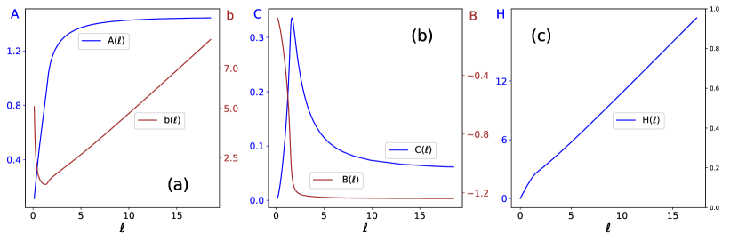
Figure 1: The fixed-point solutions of the variational equations (13). (a) amplitude of the first harmonic and width parameter; (b) amplitudes of the zeroth and second harmonic; (c) energy of the fixed point.

It is worth mentioning here that our numerical continuation algorithm determines the components of the fixed point as functions of $\omega$ (rather than $\ell$). Following the branch of fixed points that extends from $\omega_{0}=2$ to $\omega_{c}=0.417\,\omega_{0}$ before reversing to $\omega_{b}=0.527\,\omega_{0}$, we compute $\ell(\omega)=\omega b(A^{2}+\frac{8}{3}C^{2})$ (see Fig 6 in Appendix A). The functions $A(\ell)$, $B(\ell)$, $C(\ell)$, $b(\ell)$ and $H(\ell)$ in Fig 1 are then plotted as parametric curves. The asymptotic regime $\omega\to\omega_{0}$ corresponds to $\ell\to 0$; as the branch $\omega$ approaches its terminal point $\omega_{b}$, we have $\ell\to\infty$.

Returning to the partial differential equation (2), the energy of its solutions is given by

$$E[\Phi]=\frac{1}{2}\int\left[\Phi_{t}^{2}+\Phi_{x}^{2}+(\Phi^{2}-1)^{2}\right]\,dx.$$ (17)

Substituting the ansatz (7) in the integral (17) gives a time-dependent quantity that cannot be used as a bifurcation measure of the trial function (7). However when the collective coordinates $A,B,C$ and $b$ take constant values, the integral (17) becomes periodic (with period $T$). In that case, we can define the average energy carried by the configuration (7):

$${\overline{E}}=\frac{1}{T}\int_{0}^{T}E[\Phi]\,d\mathcal{T}_{0}.$$ (18)

Performing integration over $\mathcal{T}_{0}$ and $x$, equations (17) and (18) give $\overline{E}=U_{\ell}(A,B,C,b)$, where $U_{\ell}$ is as in (14b). Thus, the average field energy carried by the critical trial function (7) agrees with the energy function of the variational equations (13) evaluated at the corresponding fixed point:

$$\overline{E}(\ell)=H(\ell)=U_{\ell}\left[A(\ell),B(\ell),C(\ell),b(\ell)\right].$$ (19)

2.3 Stability of the fixed point

In order to classify the stability of the fixed points, it is sufficient to examine perturbations preserving the integral $\ell$. Linearising equations (13) and assuming the time dependence of the form

$$(\delta A,\delta B,\delta C,\delta b)^{T}=e^{(\lambda/\epsilon)\mathcal{T}_{1}}{\vec{y}},$$ (20)

where ${\vec{y}}$ is a constant 4-vector, gives a generalised eigenvalue problem

$$M{\vec{y}}=-\lambda^{2}P{\vec{y}}.$$ (21)

Here $M$ and $P$ are $4\times 4$ symmetric real matrices. The $M$ matrix is given in the Appendix B while

$$P=\left(\begin{array}[]{cccc}2b&0&0&A\\ 0&\frac{8}{3}b&0&\frac{4}{3}B\\ 0&0&\frac{4}{3}b&\frac{2}{3}C\\ A&\frac{4}{3}B&\frac{2}{3}C&P_{44}\end{array}\right),$$ (22)

$$P_{44}=\pi^{2}\frac{5A^{2}+16B^{2}+8C^{2}}{90b}+\frac{2}{3}\frac{A^{2}}{b}.$$

Note that the ansatz (20) tacitly assumes $\lambda$ being of order $\epsilon$.

The determinant of $P$ is given by

$$\det P=\frac{32b^{2}}{405}\left[5(\pi^{2}+3)A^{2}+2(4\pi^{2}-15)(2B^{2}+C^{2})\right].$$ (23)

Since $\det P>0$, Sylvester’s criterion implies that $P$ is positive definite. Therefore, all generalised eigenvalues $-\lambda^{2}$ are real and the exponents form pairs of real or pure imaginary opposite values, $\lambda$ and $-\lambda$.

The generalised eigenvalues are computed numerically; the results are in Fig 2. A pair of pure-imaginary eigenvalues emerges from the origin as $\ell$ is increased from zero. These stable eigenvalues account for the stability of the Dashen-Hasslacher-Neveu’s oscillon in the limit $\omega\to\omega_{0}$, where its slowly-varying amplitude satisfies the nonlinear Schrödinger equation. All other eigenvalues shown in Fig 2 (including three other pairs occurring for small $\ell$) are of order 1 — which is inconsistent with the ansatz (20). These eigenvalues do not carry any information on the stability properties of the oscillon and should be disregarded.

The absence of $O(\epsilon)$ eigenvalues outside the asymptotic regime $\omega\to\omega_{0}$ implies that the oscillon remains stable as $\omega$ is reduced to lower values — for as long as our variational approximation remains valid. Indeed, had the instability set in at some $\omega_{\mathrm{cr}}<\omega_{0}$, it would have brought along slowly-varying amplitude perturbations (of the periodic oscillation with the frequency $\omega_{\mathrm{cr}}$). The associated $O(\epsilon)$ eigenvalues would have been captured by the eigenvalue problem (21).

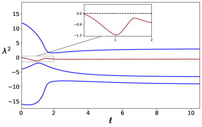
Figure 2: Roots of the characteristic equation $\det(M+\lambda^{2}P)=0$. The generalised eigenvalues $\lambda^{2}$ are shown as functions of $\ell$. The blow-up of a segment of the branch emerging from the origin highlights the fact that the eigenvalue never returns to zero.

3 Numerical standing waves

3.1 Energy-frequency diagram

To assess the accuracy of the variational approximation (7), we consider standing-wave solutions of the equation (2). The standing waves (also known as nanopterons Boyd2 and quasibreathers Fodor2 ) are temporally periodic solutions assuming prescribed values at the ends of the finite interval $-R\leq x\leq R$. Confining the analysis to spatially symmetric (even) standing waves, we determine these as solutions of a boundary-value problem posed on a rectangular domain $(0,R)\times(0,T)$. Equation (2) with the boundary conditions

$$\Phi_{x}(0,t)=\Phi(R,t)=0;\quad\Phi(x,0)=\Phi(x,T)$$ (24)

was solved by a path-following algorithm with the Newtonian iteration. The half-length of the interval, $R$, was set to $40$.

A typical solution consists of a localised core and a non-decaying small-amplitude wing, resulting from the interference of the outgoing radiation and radiation reflected by the boundary at $x=R$.

Fig 3 shows the energy

$$E_{R}[\Phi]=\int_{0}^{R}\left[\Phi_{t}^{2}+\Phi_{x}^{2}+(\Phi^{2}-1)^{2}\right]\,dx$$ (25)

of solutions of the boundary-value problem (2), (24). There are two features that attract attention in the figure.

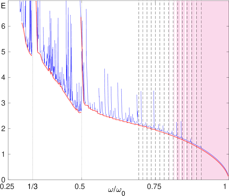
Figure 3: The energy (25) of the numerical standing-wave solution (blue). The vertical dashed lines are drawn at the subharmonic resonance frequencies $\omega=\Omega^{(n)}/2$, where $\Omega^{(n)}$ are the frequencies (27) of the linear waves. The red dotted arc underlying the numerical curve is the envelope of the family of spikes. (For visual clarity, it has been shifted down by a tiny amount from its actual position.) Clearly visible are discontinuities of the envelope at $\omega/\omega_{0}=1/2$ and $\omega/\omega_{0}=1/3$. The pink-tinted bands demarcate the frequency intervals where all Floquet multipliers lie on the unit circle.

First, the energy-frequency diagram exhibits what appears to be a sequence of spikes. On a closer examination, each “spike” turns out to consist of a pair of $E(\omega)$ branches rising steeply but not joining together. As the point $(\omega,E(\omega))$ climbs up the slope of a spike, the amplitude of the standing wave’s wing grows — this accounts for the rapid growth of the energy of the solution.

The spikes are caused by the resonance between the double frequency of the core of the standing wave and the eigenfrequencies $\Omega^{(n)}$ of the linear standing waves. The linear standing waves are given by

$$\Phi=1+\epsilon\sin(\Omega^{(n)}\mathcal{T}_{0})\cos(\kappa^{(n)}x),$$ (26)

where

$$\Omega^{(n)}=\sqrt{\omega_{0}^{2}+\left(\kappa^{(n)}\right)^{2}},\quad\kappa^{(n)}=\frac{\pi}{R}\left(n+\frac{1}{2}\right)\quad(n=0,1,2,...).$$ (27)

(Similar resonances have been detected in the three-dimensional version of the $\Phi^{4}$ model Alex_PRD .) The positions of the $\frac{1}{2}$ undertones of the linear waves are marked by the vertical dashed lines in Fig 3. One can clearly see a correspondence between the positions of the “spikes” and the points $\omega=\Omega^{(n)}/2$ through which the vertical lines are drawn.

The positions of the spikes are sensitive to the choice of the interval half-length, $R$. Let $\omega$ be a fixed frequency with $\omega_{0}/2<\omega<\omega_{0}$ and $R_{a}$ an arbitrarily chosen half-length ($R_{a}\gg 1$). Denote $k$ the wavenumber of the second-harmonic radiation, satisfying the dispersion relation

$$(n\omega)^{2}=\omega_{0}^{2}+k^{2}$$ (28)

with $n=2$. By tuning $R$ to a suitably chosen value $R_{\omega}$ within the interval $(R_{a},R_{a}+\pi/k)$, the amplitude of the “wing” can be minimized (yet not reduced to zero). The corresponding value of $E_{R}$ gives the minimum energy of the family of standing waves with frequency $\omega$: $E_{\rm min}(\omega)=E_{R_{\omega}}$. The graph of $E_{\rm min}(\omega)$ comprises segments of the $E_{R_{a}}(\omega)$ curve outside the neighbourhoods of the spikes, while the full, gapless, $E_{\rm min}(\omega)$ arc can be obtained as the envelope of the family of curves with $R$ in $(R_{a},R_{a}+\pi/k)$.

Another aspect of Fig 3 that is worth commenting on, concerns the fragmentation of the $E(\omega)$ curve into three disjoint branches with $\omega$ in the intervals $(\omega_{*},\frac{1}{3}\omega_{0})$, $(\frac{1}{3}\omega_{0},\frac{1}{2}\omega_{0})$ and $(\frac{1}{2}\omega_{0},\omega_{0})$, respectively. Here $\omega_{*}=0.289\,\omega_{0}$ is the lowest frequency value for which we obtained a solution of the boundary-value problem (2), (24). The endpoints of the intervals, $\omega_{0}/2$ and $\omega_{0}/3$, are marked by a rapid growth of the energy $E_{\rm min}$ as $\omega$ approaches these values from the right, and by finite energy jumps — as $\omega$ approaches these values from the left.

To explain the fragmentation theoretically, we turn to the dispersion relation (28). According to (28), the $n$-th harmonic radiation can only be emitted by the core oscillating with the frequency $\omega>\omega_{0}/n$. In the event of the coexistence of the $n$-th and $(n+1)$-th harmonics, the lower (the $n$-th) overtone will be energetically dominant. Therefore the radiation waves should be dominated by the second, third and fourth harmonic in the frequency ranges $(\frac{1}{2}\omega_{0},\omega_{0})$, $(\frac{1}{3}\omega_{0},\frac{1}{2}\omega_{0})$, and $(\frac{1}{4}\omega_{0},\frac{1}{3}\omega_{0})$, respectively. The harmonic waves forming the wings of our numerically obtained nanopterons do comply with this selection rule.

Raising $\omega$ through $\omega_{0}/2$ opens a channel of the quadratic radiation — a more powerful channel than the $n=3$ channel available for $\omega<\omega_{0}/2$. The amplitude of the wing increases and this explains the energy jump in Fig 3. Similarly, the energy jump observed as $\omega$ is increased through $\omega_{0}/3$ is due to the turning on of the third-harmonic channel, not accessible to the standing waves with $\omega<\omega_{0}/3$. We note that the energy jumps have the same origin as the staccato flashes of radiation from a slowly fading oscillon Dorey ; Nagy .

Assume now that $\omega$ approaches $\omega_{0}/2$ from the right. The wavelength $\lambda=2\pi/k$ of the second-harmonic radiation grows while the width of the wave’s core drops from its large values characteristic for frequencies close to $\omega_{0}$. (The decrease of $b$ as $\ell$ is raised from zero is clearly visible in the variational results of Fig 1.) The convergence of $b$ and $\lambda$ produces a resonant growth of the amplitude of the second-harmonic radiation which, in turn, gives rise to the energy hike. A similar argument explains the energy growth occurring as $\omega$ is reduced towards $\omega_{0}/3$.

3.2 Practical stability of standing waves

To classify the stability of the standing-wave solution, we linearise equation (2) about $\Phi(x,t)$:

$$y_{tt}-y_{xx}-2y+6\Phi^{2}y=0.$$ (29)

Equation (29) is supplemented with the boundary conditions

$$y_{x}(0,t)=y(R,t)=0;$$ (30)

that is, we confine our study to perturbations sharing the symmetry of the standing wave and vanishing at the same point on the $x$-line.

Having expanded $y(x,t)$ in the cosine Fourier series in the interval $(0,R)$ and keeping only the first $N$ harmonics, we have evaluated the monodromy matrix of the $T$-periodic solution for each $\omega=2\pi/T$ in Fig 3. (We took $N=512$.) If all eigenvalues $\mu_{n}$ ($n=1,2,...,2N$) of the monodromy matrix satisfy $|\mu_{n}|=1$ , the periodic solution $\Phi(x,t)$ is stable. If there are Floquet multipliers with $|\mu_{n}|>1$, the standing wave $\Phi$ is deemed linearly unstable; however, the growth of the unstable perturbations should not necessarily produce a noticeable deformation of the wave’s core.

The frequency intervals with no multipliers outside the unit circle are indicated by pink bands in Fig 3. In particular, the entire region $0.903\,\omega_{0}<\omega<\omega_{0}$ is found to be stable. As $\omega$ is continuously turned down from $0.903\,\omega_{0}$, a pair of real eigenvalues ($\mu_{m}$ and $\mu_{m}^{-1}$) repeatedly emerge and return to the unit circle. (The intervals of $\omega$ characterised by the presence of $\mu_{m}>1$ are left blank in Fig 3.) After the frequency has reached below $0.798\,\omega_{0}$, the off-circle pair remains in the Floquet spectrum for any further decrease of $\omega$.

The instability occurring in parts of the range $\omega\gtrsim 0.75\,\omega_{0}$ is weak. (Here we are assuming that the solution is not on the slope of a resonant peak). Specifically, the growth rate $\lambda=\frac{1}{T}\ln\mu_{m}$ associated with the Floquet multiplier $\mu_{m}>1$ is bounded by $3\times 10^{-3}$. As $\omega$ is decreased below $0.75\,\omega_{0}$, the unstable real eigenvalue becomes larger. In addition, complex quadruplets $\{\mu,\mu^{*},\frac{1}{\mu},\frac{1}{\mu^{*}}\}$ emerge from the unit circle.

To understand the effect of instability, we have carried out direct numerical simulations of equation (2) with initial conditions in the form of an unstable standing wave. In all cases that we examined, the evolution of the instability affected the amplitude and phase of the wing of the nanopteron, but it never led to any significant deformation of its core. Since the resulting changes would not be noticeable in most physical settings, we are referring to the standing-wave solutions of equation (2) as practically stable.

4 Numerical solution vs variational approximation

Fig 4 compares the energy of the standing wave with the average energy (19) carried by the trial function (7). In the trial function, $A,B,C$ and $b$ are taken to be the components of the fixed-point solution of equations (13). For further comparison, we have included the energy of the asymptotic solution (3),

$$E=\frac{4}{3}\epsilon+\frac{32}{81}\epsilon^{3},$$ (31)

where $\epsilon=\sqrt{\omega_{0}^{2}-\omega^{2}}$ and corrections higher than $\epsilon^{3}$ have been dropped.

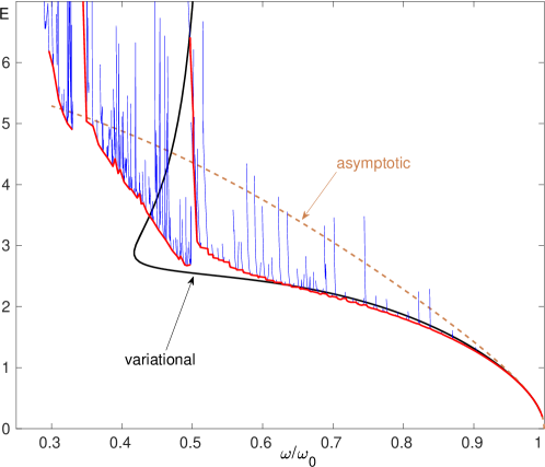
Figure 4: The energy (17) of the standing-wave solution determined numerically (blue), with the envelope curve plotted in red. (Unlike Fig 3, the envelope is shown in its true position here.) The black line depicts the average energy (19) carried by the trial function (7) with parameters given by the fixed-point of the variational equations. The dashed parabola indicates the asymptotic result (31).

In the frequency range $(0.6\,\omega_{0},\omega_{0})$, the variational ansatz (7) provides a fairly accurate approximation of the envelope of the numerical $E(\omega)$ curve. Remarkably, the variational result is much closer to $E_{\mathrm{min}}(\omega)$ than the asymptotic expansion (31). The stability of the standing wave with $\omega>0.9\,\omega_{0}$ and its practical stability for $\omega<0.9\,\omega_{0}$ are also reproduced by the variational approach.

As $\omega$ is reduced from $0.6\,\omega_{0}$ to $0.5\,\omega_{0}$, the variational $\overline{E}(\omega)$ dependence deviates from its numerical counterpart and once $\omega$ has fallen under $\omega_{0}/2$, the numerical-variational correspondence breaks down entirely. The envelope of the numerical curve in Figs 3 and 4 is split into three fragments, with $E_{\mathrm{min}}$ growing monotonically as $\omega$ decreases within each fragment. There is a unique value of $E_{\mathrm{min}}$ for each $\omega$. By contrast, the variational energy $\overline{E}(\omega)$ grows as $\omega$ is reduced from $\omega_{0}$ to $\omega_{c}=0.417\,\omega_{0}$, but then the curve turns back so that there are two coexisting branches for each $\omega$ in the interval $(\omega_{c},\omega_{b})$, where $\omega_{b}=0.527\omega_{0}$.

The numerical analysis suggests two factors that contribute to the failure of the variational approximation with low $\omega$. First, the amplitude of the radiation emitted from the core of the wave (and reflected from the boundary at $x=R$) grows as its frequency is decreased whereas the ansatz (7) does not take into account the radiation wing at all. Second, as $\omega$ is lowered below $\omega_{0}/2$, the contribution of the first harmonic to the Fourier spectrum of the core decreases while the role of higher harmonics grows. As $\omega$ falls under $0.45\,\omega_{0}$, the amplitude of the second harmonic becomes larger than, and the amplitude of the third harmonic comparable to, the amplitude of the first harmonic. When $\omega$ is under $0.4\,\omega_{0}$, both second and third harmonics make larger contributions to the dynamics than the first harmonic. As a result, the variational ansatz (7) — which keeps $\cos(\omega\mathcal{T}_{0}+\theta)$ but does not include $\cos 3(\omega\mathcal{T}_{0}+\theta)$ — becomes inadequate.

5 Concluding remarks

Any collective coordinate approach to a localised structure aims to identify the nonlinear modes that capture the essentials of its dynamics. The choice of essential coordinates is validated by the agreement between the finite-dimensional description of the structure and its true properties as revealed by the numerical analysis. In this study, we utilised the multiscale variational method to determine the nonlinear modes responsible for the formation and stability of the one-dimensional $\phi^{4}$ oscillons.

The method was previously applied BA to oscillons of the Kosevich-Kovalev model KK , defined by the Lagrangian

$$L=\frac{1}{2}\int\left(\phi_{t}^{2}-\phi_{x}^{2}-4\phi^{2}+\phi^{4}\right)dx.$$ (32)

An ansatz comprising three variables,

$$\phi=A\cos(\omega\mathcal{T}_{0}+\theta)\,\mathrm{sech}\left(\frac{x}{b}\right),$$ (33)

was found to provide an accurate agreement with the numerical simulations of the corresponding equation of motion. The $\phi^{4}$ Lagrangian of the present paper,

$$L=\frac{1}{2}\int\left(\phi_{t}^{2}-\phi_{x}^{2}-4\phi^{2}-4\phi^{3}-\phi^{4}\right)dx,$$ (34)

is different from (32) in the presence of the symmetry-breaking $\phi^{3}$ term. This term would not contribute to the effective Lagrangian generated by the trial function (33); the single-harmonic ansatz “does not see” the cubic term. To capture the asymmetry in oscillations, we have had to expand the single-harmonic ansatz (33) into a sum of three harmonics in (7). Accordingly, the number of collective variables has increased from three to five.

Our variational study was complemented by the numerical analysis of equation (2) on a periodic two-dimensional domain $(0,R)\times(0,T)$. Solutions of this boundary-value problem are standing waves consisting of a localised core and small-amplitude wings formed by the interference of the radiation emitted by the core and radiation reflected from the boundaries. We obtained solutions with all $\omega$ between $0.3\,\omega_{0}$ and $\omega_{0}$, where $\omega=2\pi/T$ is the fundamental frequency of the wave and $\omega_{0}$ is the endpoint of the continuous spectrum.

Results are summarised in Fig 3 which shows the energy of the standing wave as a function of its frequency. The diagram features a sequence of spikes generated by the resonant growth of the wing amplitude. The envelope of the family of $E_{R}(\omega)$ curves with varied $R$ gives the energy curve of the standing wave with the thinnest wings. The envelope is found to be fragmented according to the dominant radiation harmonic (second, third, or higher). Another noteworthy conclusion of the numerical analysis is the practical stability of the entire branch of standing waves.

Fig 4 attests to a good agreement between the numerical energy-frequency dependence and its variational counterpart $\overline{E}(\omega)$ in the interval $(0.6\,\omega_{0},\omega_{0})$. There also is consistency between the stability of the variational fixed point and practical stability of the standing waves.

As $\omega$ is decreased below $0.6\,\omega_{0}$, the agreement deteriorates and then breaks down completely. While the energy of the numerical solution changes monotonically within each of the three fragments of its $E(\omega)$ diagram, the variational curve turns back into a coexisting branch of fixed points (Fig 4). It remains a challenge to determine whether the standing-wave counterpart of the coexisting branch actually exists.

Appendix A Appendix: Fixed points of the variational equations

The fixed points of the dynamical system (13) satisfy four simultaneous algebraic equations

$$\frac{1}{3b^{2}}-1+A^{2}+\frac{4}{5}C^{2}+\frac{4}{5}\left(\frac{5}{2}+2B+C\right)^{2}=\omega^{2},$$ (35a)

$$\frac{1}{3}\left(5+\frac{1}{b^{2}}\right)B+\frac{5}{4}A^{2}+2B^{2}+C^{2}+\frac{1}{2}A^{2}(2B+C)+\frac{2}{7}B(2B^{2}+3C^{2})=0,$$ (35b)

$$\left(5+\frac{1}{b^{2}}\right)C+\frac{15}{4}A^{2}+12BC+3A^{2}(B+C)+\frac{9}{7}(4B^{2}+C^{2})C=5\omega^{2}C,$$ (35c)

$$\frac{5}{8}\left(4-\frac{1}{3b^{2}}\right)A^{2}+\frac{1}{3}\left(5-\frac{1}{b^{2}}\right)(2B^{2}+C^{2})+\frac{5}{2}A^{2}(2B+C)+\frac{4}{3}B(2B^{2}+3C^{2})$$

$$+\frac{5}{16}A^{4}+\frac{1}{14}(8B^{4}+3C^{4}+24B^{2}C^{2})+A^{2}(2B^{2}+C^{2}+2BC)=\frac{5}{24}\omega^{2}\left(3A^{2}+8C^{2}\right).$$ (35d)

Note that we have switched from the parametrisation by $\ell$ back to the frequency $\omega$, where

$$\omega=\frac{\ell}{b\left(A^{2}+\frac{8}{3}C^{2}\right)}.$$ (36)

While the invariant $\ell$ characterises the dynamics (in particular, stability) of solutions to equations (13), $\omega$ appears to be a more convenient parameter in the search for roots of (35).

Expressing $A^{2}$ from equation (35a) and substituting it in (35b), we obtain

$$b^{-2}=\frac{f_{\omega}(B,C)}{C+\frac{5}{2}}$$ (37)

with

$$f_{\omega}=10B+12B^{2}+6C^{2}+\frac{12}{7}B(2B^{2}+3C^{2})$$

$$+3\left(\frac{5}{2}+2B+C\right)\left[\omega^{2}+1-\frac{4}{5}C^{2}-\frac{4}{5}\left(\frac{5}{2}+2B+C\right)^{2}\right].$$ (38)

A similar substitution of $A^{2}$ in (35c) yields

$$b^{-2}=\frac{g_{\omega}(B,C)}{B+\frac{5}{4}}$$ (39)

with

$$g_{\omega}=\frac{3}{2}(1+\omega^{2})\left(\frac{5}{2}+2B-\frac{4}{3}C\right)+\left[10+12B+\frac{9}{7}(4B^{2}+C^{2})\right]C$$

$$-\frac{6}{5}\left(\frac{5}{2}+2B+2C\right)\left[\left(\frac{5}{2}+2B+C\right)^{2}+C^{2}\right],$$ (40)

while eliminating $A^{2}$ between (35a) and (35d) produces

$$b^{-4}+p_{\omega}b^{-2}+q_{\omega}=0,$$ (41)

where

$$p_{\omega}(B,C)=2\left[\frac{16}{5}\left(B+\frac{5}{4}\right)\left(C+\frac{5}{2}\right)-\omega^{2}-6\right]$$ (42)

and

$$q_{\omega}(B,C)=16\left[2B^{2}+(1-\omega^{2})C^{2}+\frac{4}{5}B(2B^{2}+3C^{2})\right.$$

$$+\left.\frac{3}{70}(8B^{4}+3C^{4}+24B^{2}C^{2})\right]-\frac{48}{25}\left[\left(\frac{5}{2}+2B+C\right)^{2}+C^{2}-\frac{5}{4}(\omega^{2}+1)\right]^{2}.$$ (43)

Before reducing the number of equations further, it is fitting to note that the system (37), (39) and (41) has a root reproducing the asymptotic expansion (3):

$$B=-\frac{\epsilon^{2}}{4},\quad C=\frac{\epsilon^{2}}{12},\quad b^{-2}=\epsilon^{2}.$$ (44)

Here we have defined a small parameter $\epsilon$ by letting, in equations (37), (39) and (41), $\omega^{2}=4-\epsilon^{2}$. Using (35a) we recover the amplitude of the first harmonic in the Dashen-Hasslacher-Neveu’s expansion:

$$A^{2}=\frac{\epsilon^{2}}{3}.$$ (45)

Returning to the system of three equations and using equation (37) to eliminate $b^{-2}$ from (39) and (41), we arrive at

$$\left(B+\frac{5}{4}\right)f_{\omega}(B,C)-\left(C+\frac{10}{4}\right)g_{\omega}(B,C)=0,$$ (46a)

$$f_{\omega}^{2}(B,C)+\left(C+\frac{10}{4}\right)p_{\omega}(B,C)f_{\omega}(B,C)+\left(C+\frac{10}{4}\right)^{2}q_{\omega}(B,C)=0.$$ (46b)

For each $\omega$, equations (46) with $f_{\omega},g_{\omega},p_{\omega},q_{\omega}$ as in (38), (40), (42) and (43), comprise a system of two equations with two unknowns, $B$ and $C$.

For much of the $\omega$, the system (46) has multiple roots with real $B$ and $C$ (Fig 5). However only roots satisfying $A^{2}>0$ and $b^{-2}>0$ correspond to fixed points of the variational equations (13). Here $b^{-2}$ is given by (37) and $A^{2}$ by equation

$$A^{2}=\frac{h_{\omega}(B,C)}{2C+5}$$ (47a)

with

$$h_{\omega}=-2B^{2}-C^{2}-B\left[\omega^{2}+\frac{8}{3}+\frac{2}{7}(2B^{2}+3C^{2})-\frac{4}{5}C^{2}-\frac{4}{5}\left(\frac{5}{2}+2B+C\right)^{2}\right],$$ (47b)

which ensues from (35a)-(35b).

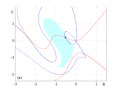
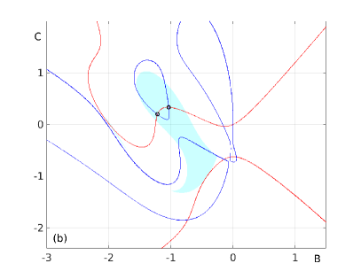
Figure 5: Graphical solution of the system (46) with $\omega=0.71\,\omega_{0}$ (a) and $\omega=0.45\,\omega_{0}$ (b). The red and blue curves are described by equations (46a) and (46b), respectively. Tinted in light blue is the “physical” region where the inequalities $A^{2}>0$ and $b^{-2}>0$ are satisfied simultaneously, with $A^{2}$ and $b^{-2}$ as in (47) and (37). Circles mark the roots of the system in the physical region.

There is only one such root for $\omega_{b}<\omega<\omega_{0}$, where $\omega_{b}=0.527\,\omega_{0}$ (and $\omega_{0}=2$). In the vicinity of $\omega_{0}$, the corresponding fixed point is given by equations (44)-(45). The branch of fixed points extends from $\omega_{0}$ to $\omega_{c}=0.417\,\omega_{0}$ where it folds onto itself. As we path-follow the turning branch back to $\omega_{b}$, the $A$, $B$ and $C$ components of the fixed point approach finite values while $b$ grows without bound. As a result, the adiabatic invariant $\ell=\omega b(A^{2}+\frac{8}{3}C^{2})$ and the energy (16) tend to infinity as well (Fig 6).

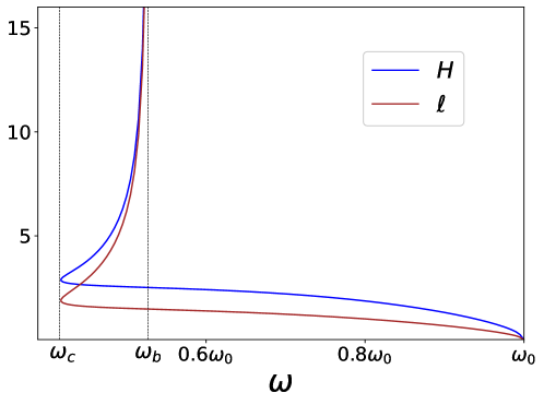
Figure 6: The adiabatic invariant $\ell$ and energy $H$ of the fixed point as functions of $\omega$.

Appendix B Appendix: Linearisation matrix

The matrix elements $M_{ij}=M_{ji}$ in equation (21) are given by

$$M_{11}=24\omega^{2}\frac{A^{2}b}{3A^{2}+8C^{2}}+\frac{2}{3b}+2b\left[3A^{2}+\frac{4}{5}\left(\frac{5}{2}+2B+C\right)^{2}+\frac{4C^{2}}{5}-\omega^{2}-1\right];$$

$$M_{12}=\frac{32}{5}Ab\left(\frac{5}{2}+2B+C\right);\quad M_{13}=64\omega^{2}\frac{ACb}{3A^{2}+8C^{2}}+\frac{16}{5}Ab\left(\frac{5}{2}+2B+2C\right);$$

$$M_{14}=4\omega^{2}A+\frac{8}{5}A\left(\frac{5}{2}+2B+C\right)^{2}+2A\left(A^{2}+\frac{4C^{2}}{5}-\frac{1}{3b^{2}}-\omega^{2}-1\right);$$

$$M_{22}=\frac{32}{5}A^{2}b+\frac{32}{15b}+\frac{32}{105}b\left[36\left(B+\frac{7}{6}\right)^{2}+18C^{2}-14\right];\quad M_{23}=\frac{16}{35}b\left(7A^{2}+24CB+28C\right);$$

$$M_{24}=\frac{16}{5}A^{2}\left(\frac{5}{2}+2B+C\right)+\frac{192}{35}\left(B+\frac{7}{6}\right)C^{2}+\frac{8}{15}B\left[\frac{48}{7}\left(B+\frac{7}{4}\right)^{2}-1\right]-\frac{32}{15}\frac{B}{b^{2}};$$

$$M_{33}=\frac{512}{3}\omega^{2}\frac{C^{2}b}{3A^{2}+8C^{2}}+\frac{192}{35}b\left(B+\frac{7}{6}\right)^{2}+\frac{16}{15b}+\frac{16}{105}b\left(21A^{2}+27C^{2}-35\omega^{2}-14\right);$$

$$M_{34}=\frac{32}{3}\omega^{2}C+\frac{48}{35}C^{3}+\frac{16}{15}\left[3A^{2}+\frac{36}{7}\left(B+\frac{7}{6}\right)^{2}-5\omega^{2}-2\right]C+\frac{16}{5}A^{2}\left(B+\frac{5}{4}\right)-\frac{16}{15}\frac{C}{b^{2}};$$

$$M_{44}=\frac{2}{3}\frac{\omega^{2}}{b}(3A^{2}+8C^{2})+\frac{2}{15b^{3}}\left(5A^{2}+16B^{2}+8C^{2}\right).$$ (48)

Here $A,B,C$ and $b$ are components of the real root of the system (35).

Note that the linearisation of equations (13) preserves $\ell$: $\delta\ell=0$. The frequency $\omega$ does not appear in (13) but once the linearisation procedure has been completed, we reintroduce $\omega$ according to

$$\omega=\frac{\ell}{b\left(A^{2}+\frac{8}{3}C^{2}\right)},$$

in agreement with (36). In the matrix elements (48), the variables $A,B,C$ and $b$ are single-valued functions of $\ell$ — and $\omega$ is also considered as a function of $\ell$.

References

- (1) N A Voronov, I Y Kobzarev, and N B Konyukhova, Possibility of the existence of X mesons of a new type. JETP Lett 22 290 (1975)
- (2) I L Bogolyubskii and V G Makhankov, On the pulsed soliton lifetime in two classical relativistic theory models. JETP Lett 24 12 (1976)
- (3) I L Bogolyubskii and V G Makhankov, Dynamics of spherically symmetrical pulsons of large amplitude. JETP Lett 25 107 (1977)
- (4) M Gleiser, Pseudostable bubbles. Phys Rev D 49 2978 (1994)
- (5) E J Copeland, M Gleiser and H-R Müller, Oscillons: Resonant configurations during bubble collapse. Phys Rev D 52 1920 (1995)
- (6) Ya. B. Zel’dovich, I. Yu. Kobzarev, and L. B. Okun’. Cosmological consequences of a spontaneous breakdown of a discrete symmetry. Sov. Phys.-JETP 40 1 (1975)
- (7) A Riotto, Oscillons are not present during a first order electroweak phase transition. Phys Lett B 365 64 (1996)
- (8) I. Dymnikova, L. Koziel, M. Khlopov, and S. Rubin, Quasilumps from first order phase transitions. Gravitation and Cosmology 6 311 (2000)
- (9) M. Broadhead and J. McDonald, Simulations of the end of supersymmetric hybrid inflation and nontopological soliton formation. Phys. Rev. D 72 043519 (2005)
- (10) M Gleiser, Oscillons in scalar field theories: applications in higher dimensions and inflation. Int. J. Mod. Phys. D 16 219 (2007)
- (11) E. Farhi, N. Graham, A. H. Guth, N. Iqbal, R. R. Rosales, and N. Stamatopoulos, Emergence of oscillons in an expanding background. Phys. Rev. D 77 085019 (2008)
- (12) M. Gleiser, B. Rogers, and J. Thorarinson, Bubbling the false vacuum away. Phys. Rev. D 77 023513 (2008)
- (13) M. A. Amin, Inflaton fragmentation: Emergence of pseudo-stable inflaton lumps (oscillons) after inflation. arXiv:1006.3075 (2010)
- (14) M Gleiser, N Graham, and N Stamatopoulos, Generation of coherent structures after cosmic inflation. Phys Rev D 83 096010 (2011)
- (15) M. A. Amin, R. Easther, H. Finkel, R. Flauger and M.P. Hertzberg, Oscillons after inflation. Phys. Rev. Lett. 108 241302 (2012)
- (16) S-Y Zhou, E J Copeland, R Easther, H Finkel, Z-G.Moua and P M Saffin, Gravitational waves from oscillon preheating. JHEP 10 026 (2013)
- (17) M Gleiser and N Graham, Transition to order after hilltop inflation. Phys Rev D 89 083502 (2014)
- (18) P. Adshead, J. T. Giblin Jr., T. R. Scully and E. I. Sfakianakis, Gauge-preheating and the end of axion inflation. Journ of Cosmology and Astroparticle Physics, 12 034 (2015)
- (19) J R Bond, J Braden and L Mersini-Houghton, Cosmic bubble and domain wall instabilities III: the role of oscillons in three-dimensional bubble collisions. Journ Cosmology and Astroparticle Physics 09 004 (2015)
- (20) S Antusch, F. Cefalà and S Orani, Gravitational waves from oscillons after inflation. Phys Rev Lett 118 011303 (2017)
- (21) J-P Hong, M Kawasaki, and M Yamazaki, Oscillons from pure natural inflation. Phys Rev D 98 043531 (2018)
- (22) K. D. Lozanov and M. A. Amin, Gravitational perturbations from oscillons and transients after inflation. Phys. Rev. D 99 123504 (2019)
- (23) D Cyncynates and T Giurgica-Tiron. Structure of the oscillon: The dynamics of attractive self-interaction. Phys Rev D 103 116011 (2021)
- (24) K D Lozanov and V Takhistov. Enhanced Gravitational Waves from Inflaton Oscillons. Phys. Rev. Lett. 130 181002 (2023)
- (25) J. C. Aurrekoetxea, K. Clough, and F. Muia. Oscillon formation during inflationary preheating with general relativity. Phys. Rev. D 108 023501 (2023)
- (26) E. Farhi, N. Graham, V. Khemani, R. Markov, R. Rosales, An oscillon in the SU(2) gauged Higgs model. Phys. Rev. D 72 (2005) 101701(R);
- (27) N. Graham, An Electroweak Oscillon. Phys. Rev. Lett. 98 (2007) 101801; Numerical simulation of an electroweak oscillon. Phys. Rev. D 76 (2007) 085017;
- (28) M Gleiser, N Graham, and N Stamatopoulos, Long-lived time-dependent remnants during cosmological symmetry breaking: From inflation to the electroweak scale. Phys Rev D 82 043517 (2010);
- (29) E. I. Sfakianakis, Analysis of oscillons in the SU(2) gauged Higgs model. arXiv:1210.7568 (2012)
- (30) M Piani and J Rubio. Preheating in Einstein-Cartan Higgs Inflation: oscillon formation. JCAP 12 002 (2023)
- (31) E. W. Kolb and I. I. Tkachev, Nonlinear axion dynamics and the formation of cosmological pseudosolitons. Phys. Rev. D 49 5040 (1994)
- (32) A Vaquero, J Redondo and J Stadler, Early seeds of axion miniclusters. Journ of Cosmology and Astroparticle Physics 04 012 (2019)
- (33) M Kawasaki, W Nakanoa, and E Sonomoto, Oscillon of ultra-light axion-like particle. Journ of Cosmology and Astroparticle Physics 01 047 (2020)
- (34) J Olle, O Pujolas, and F Rompineve, Oscillons and dark matter. Journ of Cosmology and Astroparticle Physics 02 006 (2020)
- (35) A Arvanitaki, S Dimopoulos, M Galanis, L Lehner, J O Thompson, and K Van Tilburg, Large-misalignment mechanism for the formation of compact axion structures: Signatures from the QCD axion to fuzzy dark matter. Phys Rev D 101 083014 (2020)
- (36) M Kawasaki, K Miyazaki, K Murai, H Nakatsuka, E Sonomoto, Anisotropies in cosmological 21 cm background by oscillons/ I-balls of ultra-light axion-like particle. Journ of Cosmology and Astroparticle Physics 08 066 (2022)
- (37) S Antusch, F Cefalà, S Krippendorf, F Muia, S Orani and F Quevedo, Oscillons from string moduli. JHEP 01 083 (2018)
- (38) Y Sang and Q-G Huang, Stochastic gravitational-wave background from axion-monodromy oscillons in string theory during preheating. Phys. Rev. D 100 063516 (2019)
- (39) S Kasuya, M Kawasaki, F Otani, and E Sonomoto, Revisiting oscillon formation in the Kachru-Kallosh-Linde-Trivedi scenario. Phys Rev D 102 043016 (2020)
- (40) K Imagawa, M Kawasaki, K Murai, H Nakatsuka and E Sonomoto. Free streaming length of axion-like particle after oscillon/-ball decays. JCAP 02 024 (2023)
- (41) V. A. Koutvitsky and E. M. Maslov, Gravipulsons. Phys Rev D 83 124028 (2011); Passage of test particles through oscillating spherically symmetric dark matter configurations. Phys Rev D 104 124046 (2021)
- (42) H-Y Zhang, Gravitational effects on oscillon lifetimes. Journ of Cosmology and Astroparticle Physics 03 102 (2021)
- (43) Z Nazari, M Cicoli, K Clough and F Muia, Oscillon collapse to black holes. Journ of Cosmology and Astroparticle Physics 05 027 (2021)
- (44) X-X Kou, C Tian and S-Y Zhou, Oscillon preheating in full general relativity. Class. Quantum Grav. 38 045005 (2021)
- (45) T Hiramatsu, E I Sfakianakis and M Yamaguchi, Gravitational wave spectra from oscillon formation after inflation. Journ High Energy Phys 21 2021 (2021)
- (46) X-X Kou, J B Mertens, C Tian and S-Y Zhou, Gravitational waves from fully general relativistic oscillon preheating. Phys Rev D 105 123505 (2022)
- (47) K Nakayama, F Takahashia and M Yamada. Quantum decay of scalar and vector boson stars and oscillons into gravitons. JCAP 08 058 (2023)
- (48) A E Kudryavtsev. Solitonlike solutions for a Higgs scalar field. JETP Lett 22 82 (1975)
- (49) R F Dashen, B Hasslacher and A Neveu, Particle spectrum in model field theories from semiclassical functional integral techniques. Phys Rev D 11 3424 (1975)
- (50) B S Getmanov. Bound states of solitons in the field theory. JETP Lett 24 291 (1976)
- (51) T. Sugiyama, Kink-Antikink collisions in the two-dimensional model. Prog. Theor. Phys. 611550 (1979)
- (52) J Geicke. How stable are pulsons in the field theory? Phys Lett B 133 337 (1983)
- (53) D. K. Campbell, M.Peyrard. Solitary wave collisions revisited. Physica D 18 47 (1986)
- (54) E P Honda and M W Choptuik, Fine structure of oscillons in the spherically symmetric Klein-Gordon model. Phys Rev D 65 084037 (2002)
- (55) G Fodor, P Forgácz, P Grandclément, and I Rácz, Oscillons and quasibreathers in the Klein-Gordon model. Phys Rev D 74 124003 (2006)
- (56) G. Fodor. A review on radiation of oscillons and oscillatons. arXiv:1911.03340 [hep-th]
- (57) T I Belova, A E Kudryavtsev. Solitons and their interactions in classical field theory. Physics - Uspekhi 40 359 (1997)
- (58) H Segur and M D Kruskal. Nonexistence of Small-Amplitude Breather Solutions in Theory. Phys Rev Lett 58 747 (1987)
- (59) S Dutta, D A Steer, T Vachaspati. Creating kinks from particles. Phys Rev Lett 101 121601 (2008)
- (60) S. Rychkov and L. G. Vitale, Hamiltonian truncation study of the theory in two dimensions. II. The -broken phase and the Chang duality, Phys. Rev. D 93, 065014 (2016)
- (61) Z. Bajnok and M. Lajer, Truncated Hilbert space approach to the 2d theory, J. High Energy Phys. 10 050( 2016)
- (62) M. Serone, G. Spada, and G. Villadoro, theory—Part II. The broken phase beyond NNNN(NNNN)LO, J. High Energy Phys. 05 047 (2019)
- (63) M Bordag. Vacuum Energy for a Scalar Field With Self-Interaction in (1 + 1) Dimensions. Universe 7 55 (2021)
- (64) N. Graham, H. Weigel. Quantum Corrections to Soliton Energies. Int. J. Mod. Phys. A 37 2241004 (2022)
- (65) D. Szász-Schagrin and G. Takács. False vacuum decay in the (1 + 1)-dimensional theory. Phys Rev D 106 025008 (2022)
- (66) M A A Martin, R Schlesier, J Zahn. The semiclassical energy density of kinks and solitons. Phys. Rev. D 107 065002 (2023)
- (67) H Ito, M Kitazawa. Gravitational form factors of a kink in 1+1 dimensional model . JHEP 08 033 (2023)
- (68) J Dziarmaga, P Laguma and W H Zurek. Symmetry Breaking with a Slant: Topological Defects after an Inhomogeneous Quench. Phys Rev Lett 82 4749 (1999)
- (69) F Suzuki and W H Zurek. Topological defect formation in a phase transition with tunable order. ArXiv:2312.01259 [cond-mat.stat-mech]
- (70) V. M. Eleonskii, N. E. Kulagin, N. S. Novozhilova, and V. P. Silin. Asymptotic expansions and qualitative analysis of finite-dimensional models in nonlinear field theory. Theor Math Phys 60 896 (1984)
- (71) J P Boyd. A numerical calculation of a weakly non-local solitary wave: the breather. Nonlinearity 3 177 (1990)
- (72) G Fodor, P Forgács, Z Horváth, and M Mezei. Computation of the radiation amplitude of oscillons. Phys Rev D 79 065002 (2009)
- (73) J P Boyd. Continuum Breathers: Forty Years After. In: A Dynamical Perspective on the Model. Past, Present and Future. P. G. Kevrekidis and J Cuevas-Maraver, Editors. Nonlinear Systems and Complexity vol. 26. Springer Nature, Switzerland (2019). https://doi.org/10.1007/978-3-030-11839-6
- (74) B A Malomed. Variational methods in nonlinear fiber optics and related fields. Progress in Optics 43 71 (2002)
- (75) I V Barashenkov, N V Alexeeva, E V Zemlyanaya. Two- and three-dimensional oscillons in nonlinear Faraday resonance. Phys Rev Lett 89 104101 (2002)
- (76) I V Barashenkov and N V Alexeeva. Variational formalism for the Klein-Gordon oscillon. Phys Rev D 108 096022 (2023)
- (77) P. G. Kevrekidis, R. Carretero-González, J. Cuevas-Maraver, D. J. Frantzeskakis, J.-G. Caputo, B. A. Malomed. Breather stripes and radial breathers of the two-dimensional sine-Gordon equation. Commun Nonlinear Sci Numer Simulat 94 (2021) 105596
- (78) J G Caputo and N Flytzanis, Kink-antikink collisions in sine-Gordon and models: Problems in the variational approach. Phys Rev A 44 6219 (1991)
- (79) N V Alexeeva, I V Barashenkov, A. A. Bogolubskaya and E. V. Zemlyanaya. Understanding oscillons: Standing waves in a ball. Phys Rev D 107 076023 (2023)
- (80) P. Dorey, T. Romańczukiewicz, Y. Shnir. Staccato radiation from the decay of large amplitude oscillons. Phys Lett B 806 135497 (2020)
- (81) B. C. Nagy and G. Takacs. Collapse instability and staccato decay of oscillons in various dimensions. Phys Rev D 104 056033 (2021)
- (82) A. M. Kosevich and A. S. Kovalev. Self-localization of vibrations in a one-dimensional anharmonic chain. Sov Phys JETP 40 891 (1975)