Make Continual Learning Stronger via C-Flat

Abstract

Model generalization ability upon incrementally acquiring dynamically updating knowledge from sequentially arriving tasks is crucial to tackle the ’sensitivity-stability’ dilemma in Continual Learning (CL). Weight loss landscape sharpness minimization seeking for flat minima lying in neighborhoods with uniform low loss or smooth gradient is proven to be a strong training regime improving model generalization compared with loss minimization based optimizer like SGD. Yet only a few works have discussed this training regime for CL, proving that dedicated designed zeroth-order sharpness optimizer can improve CL performance. In this work, we propose a Continual Flatness (C-Flat) method featuring a flatter loss landscape tailored for CL. C-Flat could be easily called with only one line of code Make Continual Learning Stronger via C-Flat and is plug-and-play to any CL methods. A general framework of C-Flat applied to all CL categories and a thorough comparison with loss minima optimizer and flat minima based CL approaches is presented in this paper, showing that our method can boost CL performance in almost all cases. Code will be publicly available upon publication.

C-Flat: just a line of code suffices for its utilization.

⬇

1from … import C_Flat

2

3# initialize optimizer for CL.

4C_Flat_optimizer = C_Flat(params, base_optimizer, model, args)

1 Introduction

Why study Continual Learning (CL)? CL is generally acknowledged as a necessary attribute for Artificial General Intelligence (AGI) [22, 52, 39, 59, 15]. In the open world, CL holds the potential for substantial benefits across many applications: e.g. vision model needs to learn a growing images set [16, 58], or, embodied model needs to incrementally add skills to their repertoire [68, 11, 17].

Challenges. A good CL model is expected to keep memory of all seen tasks upon learning new knowledge [22]. However, given limited access to the previous data, CL suffers from a phenomenon called catastrophic forgetting [8], which refers to the drastic performance drop on past knowledge after learning new knowledge. How to improve the model generalization ability for a stable learning performance on diverse tasks arriving sequentially is the key to overcome this major challenge in CL.

Current solutions. A series of works [41, 42, 33, 25, 57] are proposed to improve learning stability by extending data space with dedicated selected and stored exemplars from old tasks, or frozen some network blocks or layers that are strongly related to previous knowledge [65, 24, 66, 54, 24].

Another group of works seeks to preserve model generalization with regulations onto the training procedure itself [32, 18, 31]. Diverse weight [43, 28, 2] or gradient alignment [22, 8, 35, 26] strategies are designed to encourage the training to efficiently extracting feathers for the current data space without forgetting.

Loss landscape sharpness optimization [23, 19, 62, 67] as an efficient training regime for model generalization starts to gain attentions [27]. While loss minima based optimizer like SGD can easily lead to suboptimal result [4, 37, 12], zeroth-order sharpness minimization seeks flat minima that lie in neighborhood with uniform low loss [20]. Furthermore, the first-order flatness constraining the uniform curvature of the loss landscape is proposed to characterize the generalization in the standard setting [60].

Some CL works [47, 30] have already shown that zeroth-order sharpness related optimization dedicated designed for certain algorithm or application can help overcoming catastrophic forgetting in corresponding scenarios [9, 47].

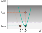
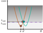
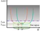
Our solution. Inspired by these works, we propose a continual flatness optimization method where maximal neighborhood loss value and curvature regularization are introduced to mitigate the generalization gap between previous and current knowledge space during CL. We dub this method Continual Flatness (C-Flat or $C\flat$ derived from music-a pitch that is one semitone lower than $C$). Moreover, C-Flat is a general method that can be be easily plug-and-play onto any CL approach with only one line of code Make Continual Learning Stronger via C-Flat, to improve CL.

Contribution. A simple but flexible to use CL optimizer is proposed that goes beyond zeroth-order sharpness to Make Continual Learning Stronger.

A framework of C-Flat covering divers CL method categories together with the corresponding comparison with vanilla optimizer and zeroth-order sharpness approaches are demonstrated in this paper. Experiment results proves that Flatter is Better in nearly all cases.

To the best of our knowledge, this work is the first to conduct a thorough comparison of CL approaches with loss landscape aware optimization, and thus can server as a baseline in this field.

(a)

(b)

(c)

(d) *

Figure 1: Illustration of C-Flat overcoming catastrophe forgetting by fine-tuning the old model parameter to flat minima of new task. a): loss minima for current task only can cause catastrophe forgetting on previous ones. b): balanced optima aligned by regularization may lead to unsatisfying result for both old and new tasks. c): C-Flat seeks global optima for all tasks with flattened loss landscape.

2 Related work

Continual learning methods roughly are categorized into three groups: Memory-based methods write experience in memory to alleviate forgetting. Some work [41, 42, 25, 49] design different sampling strategies to establish limited budgets in a memory buffer for rehearsal. However, these methods require access to raw past data, which is discouraged in practice due to privacy concerns. Instead, recently a series of works [9, 34, 44, 33, 48] elaborately construct special subspace of old tasks as the memory. Regularization-based methods aims to realize consolidation of the previous knowledge by introducing additional regularization terms in the loss function. Some works [32, 29, 6] enforce the important weights in the parameter space [43, 28, 2], feature representations [5, 21], or the logits outputs [32, 40] of the current model function to be close to that of the old one. Expansion-based methods dedicate different incremental model structures towards each task to minimize forgetting [65]. Some work [46, 24, 56] exploit modular network architectures (dynamically extending extra components [54, 66], or freeze partial parameters [36, 1]) to overcome forgetting. Trivially, methods in this category implicitly shifts the burden of storing numerous raw data into the retention of model [65].

Gradient-based solutions a.k.a the problem at the source [22, 8]. Motivated by the tug-of-war learning dynamics during optimization, one promising solution is to modify the gradients of different tasks to overcome forgetting [7, 38], e.g., aligning the gradients of current and old one [14, 18], or, learning more efficient in the case of conflicting objectives [45, 53, 13]. Other solution [9, 47] focus on characterizing the generalization from the loss landscape perspectives to improve CL performance, and yet, this sort of solution is rarely explored.

Sharpness minimization in CL Many recent works [23, 19, 4] are proposed to optimize neural networks in standard training scenarios towards flat minima. In CL, the flat minima also are proven to be effective for mitigating catastrophic forgetting [9, 47]. For example, FS-DPGM [9] proposed a dynamic gradient memory projection method using sharpness evaluation to address the ’sensitivity-stability’ dilemma in pseudo rehearsal based CL. F2M [47] introduced a fine tuning strategy for the model parameters within the flatness minima regions only in the base session for incremental few-shot learning. These efforts kicked off the study of flat minima in CL by proving that sharpness-aware minimization [20] can improve the performance of incremental class learning, but the current works consider zeroth-order sharpness only, while the application scenario is limited. The practical methods that beyond zeroth-order flatness in CL will be further studied in this work.

3 Method

In this section, we present a joint loss landscape sharpness aware optimization for CL, namely C-Flat, in Subsec. 3.1. Subsec. 3.2 introduces how can our C-Flat easily plug-and-play onto any CL methods with corresponding solutions.

Notations Continual learning is to get a generalized model from data of different distributions dynamically arriving in sequences. Let $D^{t}=(\mathscr{X}^{t}\times\mathscr{Y}^{t})$ represent the data distribution on at time $t=1,\cdots,T$, where $\mathscr{X}^{t}$ and $\mathscr{Y}^{t}$ are the input data and corresponding label spaces, and $S^{t}=\{(x_{i}^{t},y_{i}^{t})\}^{n^{t}}_{i=1}$ denotes the training set with $n^{t}$ samples independently drawn from data space $D^{t}$. Let $f^{t}$ denotes the model trained at time $t$ with parameter $\theta^{t}\in\Theta\subset\mathbb{R}^{d}$, and $\mathscr{l}:\Theta\times\mathscr{X}\times\mathscr{Y}$ an arbitrary loss function. The goal of CL is to find the optimized model $f^{T}$ that controls the statistical risk of all seen tasks given limited or no access to data $S^{t}=\{(X^{t},Y^{t})\}$ from previous tasks $t<T$:

$$f^{T}=\mathop{\arg\min}\limits_{f}\sum_{t=1}^{t=T}\mathbb{E}_{(\mathscr{X}^{t}\times\mathscr{Y}^{t})}[\mathscr{l}(f(\mathscr{X}^{t};\theta^{T}),\mathscr{Y}^{t})].$$ (1)

For the current task at time $T$, it can be approximated by the empirical risk:

$$f^{T}=\mathop{\arg\min}\limits_{f}\frac{1}{n^{t}}\sum_{i=1}^{i=n^{t}}\mathscr{l}(f(x_{i}^{t};\theta^{T}),y_{i}^{t}).$$ (2)

3.1 C-Flat: Continual Flatness Method

Model generalization is a severe task in CL for joint learning knowledge obtained from different catalogues domains or tasks. Various approaches using diverse memory replay, regularization or model expansion strategies are proposed to balance the learning stability and sensitivity when adopting new knowledge. Gradient landscape sharpness, i.e., zeroth-order sharpness has been proved to be effective in certain CL methods to mitigate forgetting. In this work, a general but stranger optimization method enhanced by the latest gradient landscape flatness is proposed as a ’plug-and-play’ tool to any CL approach.

Definition. Let $B(\theta,\rho)=\{\theta^{\prime}:\|\theta^{\prime}-\theta\|<\rho\}$ denotes the neighborhood of $\theta$ with radius $\rho>0$ in the the Euclidean space $\Theta\subset\mathbb{R}^{d}$, the zeroth-order sharpness at point $\theta$ is commonly defined by the maximal training loss difference within its neighborhood $B(\theta,\rho)$:

$$R^{0}_{\rho}(\theta)=max\{\mathscr{l}_{S}(\theta^{\prime})-\mathscr{l}_{S}(\theta):\theta^{\prime}\in B(\theta,\rho)\}.$$ (3)

where $\mathscr{l}_{S}(\theta)$ denotes the loss of an arbitrary model with parameter $\theta$ on any dataset $S$ with an oracle loss function $\mathscr{l}(\cdot)$. The zeroth-order sharpness $R^{0}_{\rho}(\theta)$ regularization can be directly applied to restrain the maximal neighborhood training loss:

$$\mathscr{l}^{R^{0}_{\rho}}_{S}(\theta)=\mathscr{l}_{S}(\theta)+R^{0}_{\rho}(\theta)=max\{\mathscr{l}_{S}(\theta^{\prime}):\theta^{\prime}\in B(\theta,\rho)\},$$

Recently, first-order gradient landscape flatness is proposed as a measurement of the maximal neighborhood gradient norm, which reflects landscape curvature, to better describe the smoothness of the loss landscape, which is defined as follows,

$$R^{1}_{\rho}(\theta)=\rho\cdot\max\{\|\nabla\mathscr{l}_{S}(\theta^{\prime})\|_{2}:\theta^{\prime}\in B(\theta,\rho)\}.$$ (4)

The direct sum of the zeroth-order sharpness with loss is enough to force the training converge to a local minimal. However, the first-order flatness constraining on the gradient norm can not guarantee to be an optimal with minimal loss. Therefore, a hyperparameter $\lambda$ is required to balance the influence of $R^{1}_{\rho}$ as an additional regularization to loss function $\mathscr{l}$:

$$\mathscr{l}^{R^{1}_{\rho}}_{S}(\theta)=\mathscr{l}_{S}(\theta)+\lambda R^{1}_{\rho}(\theta).$$ (5)

To maximize the generalization ability of loss landscape sharpness for continual learning task, we propose a zeroth-first-order sharpness aware optimizer C-Flat for CL. Considering the data space, model or blocks to be trained are altered regarding the training phase and CL method, (as detailed in the next subsection), we define the the C-Flat loss as follows:

$$\mathscr{l}_{S^{T}}^{C}(f^{T}(\theta^{T})) =\mathscr{l}_{S^{T}}(f^{T}(\theta^{T}))+R^{0}_{\rho,S^{T}}(f^{T}(\theta^{T}))+\lambda\cdot R^{1}_{\rho,S^{T}}(f^{T}(\theta^{T}))$$

$$=\mathscr{l}_{S^{T}}^{R^{0}_{\rho}}(f^{T}(\theta^{T}))+\lambda\cdot R^{1}_{\rho,S^{T}}(f^{T}(\theta^{T})),$$ (6)

with the minimization objective:

$$\arg\min_{\theta^{T}}\{\arg\max_{\theta^{T}_{0}}\mathscr{l}_{S^{T}}(f^{T}(\theta^{T}_{0}))+\lambda\rho\cdot\arg\max_{\rho_{1}}\|\bigtriangledown\mathscr{l}_{S^{T}}(f^{T}(\theta^{T}_{1}))\|_{2}$$

$$:\theta^{T}_{0},\theta^{T}_{1}\in B(\theta^{T},\rho)\}$$ (7)

where $\mathscr{l}^{R^{0}_{\rho}}_{S}(\theta)$ is constructed to replace the original CL loss, while $R^{1}_{\rho}(\theta)$ further regularizes the smoothness of the neighborhood. Hence, the local minima within a flat and smooth neighborhood is calculated for a generalized model possessing both old and new knowledge.

Optimization. In our work, the two regularization terms in the proposed C-Flat are resolved correspondingly in each iteration. Assuming the loss function $\mathscr{l}(\cdot)$ is differentiable and bounded, the gradient of $\mathscr{l}^{R^{0}_{\rho}}_{S}$ at point $\theta^{T}$ can be approximated by

$$\bigtriangledown\mathscr{l}^{R^{0}_{\rho}}_{S}(\theta^{T})\approx\bigtriangledown\mathscr{l}_{S}(\theta^{T}_{0})\text{\, with }\theta^{T}_{0}=\theta^{T}+\rho\cdot\text{sign}(\bigtriangledown\mathscr{l}_{S}(\theta^{T}))\cdot\frac{|\bigtriangledown\mathscr{l}_{S}(\theta^{T})|}{\|\bigtriangledown\mathscr{l}_{S}(\theta^{T})\|_{2}}$$ (8)

where $|\cdot|$ denotes elementwise absolute value. And the gradient of the first-order flatness regularization $\bigtriangledown R^{1}_{\rho}(\theta^{T})$ can be approximated by

$$\bigtriangledown R^{1}_{\rho}(\theta^{T})\approx\rho\cdot\bigtriangledown\|\bigtriangledown\mathscr{l}_{S}(\theta^{T}_{1})\|_{2}$$ (9)

with $$\theta^{T}_{1}=\theta^{T}+\rho\cdot\frac{\bigtriangledown\|\bigtriangledown\mathscr{l}_{S}(\theta^{T})\|_{2}}{\Large\|\bigtriangledown\|\bigtriangledown\mathscr{l}_{S}(\theta^{T})\|_{2}\Large\|_{2}}$$

where $$\bigtriangledown\|\bigtriangledown\mathscr{l}_{S}(\theta^{T})\|_{2}=\bigtriangledown^{2}\mathscr{l}_{S}(\theta^{T})\cdot\frac{\bigtriangledown\mathscr{l}_{S}(\theta^{T})}{\|\bigtriangledown\mathscr{l}_{S}(\theta^{T})\|_{2}}.$$

The optmization is detailed in  Algorithm 1. Note that $\bigtriangledown\mathscr{l}$ is the gradient of $\mathscr{l}$ with respect to $\theta$ through this paper, and instead of the expensive computation of Hessian matrix $\nabla^{2}\mathscr{l}$, Hessian-vector product calculation is used in our algorithm, where the time and especially space complexity are greatly reduced to $o(n)$.

Algorithm 1 C-Flat Optimization

Input: Training phase $T$, training data $S^{T}$, model $f^{T-1}$ with parameter $\theta^{T-1}$ from last phase if $T>1$, batch size $b$, oracle loss function $\mathscr{l}$, learning rate $\eta>0$, neighborhood size $\rho$, trade-off coefficient $\lambda$, small constant $\xi$.

Output: Model trained at the current time $T$ with C-Flat.

Initialization:

if T=1: then Randomly Initialize parameter $\theta^{T=1},\eta^{T=1}=\eta,\rho^{T=1}=\rho$.

else

     Reconstruct the model and training set if necessary,

     Initialize model parameter $\theta^{T}=\theta^{T-1},\eta^{T}=\eta,\rho^{T}=\rho$,

     Frozen part of the parameter if required.

end if

Optimization:

while $\theta^{T}$ not converge, do

     Sample batch $B^{T}$ of $b$ random instances from $S^{T}$

     Compute batch’s loss gradient $\bigtriangledown\mathscr{l}_{B^{T}}(f^{T}({\theta^{T}}))$

     Compute $R^{0}_{\rho}$ perturbation: $\epsilon_{0}=\rho^{T}\cdot\text{sign}(\bigtriangledown\mathscr{l}_{B^{T}}(f^{T}({\theta^{T}}))\cdot\frac{|\bigtriangledown\mathscr{l}_{B^{T}}(f^{T}({\theta^{T}}))|}{\|\bigtriangledown\mathscr{l}_{B^{T}}(f^{T}({\theta^{T}}))\|_{2}+\epsilon}$

     Compute zeroth-order gradient approximation: $h_{0}=\bigtriangledown\mathscr{l}_{B^{T}}(f^{T}({\theta^{T}}+\epsilon_{0}))$

     Compute $h=\bigtriangledown^{2}\mathscr{l}_{S}(\theta)\cdot\frac{\bigtriangledown\mathscr{l}_{B^{T}}(f^{T}({\theta^{T}}))}{\|\bigtriangledown\mathscr{l}_{B^{T}}(f^{T}({\theta^{T}}))\|_{2}+\epsilon}$

     Compute $R^{1}_{\rho}$ perturbation: $\epsilon_{1}=\rho^{T}\cdot\frac{\bigtriangledown\|\bigtriangledown\mathscr{l}_{B^{T}}(f^{T}({\theta^{T}}))\|_{2}}{\Large\|\bigtriangledown\|\bigtriangledown\mathscr{l}_{B^{T}}(f^{T}({\theta^{T}}))\|_{2}\Large\|_{2}+\epsilon}$

     Compute first-order gradient approximation: $h_{1}=\bigtriangledown^{2}\mathscr{l}_{B^{T}}(f^{T}({\theta^{T}}+\epsilon_{1}))\cdot\frac{\bigtriangledown\mathscr{l}_{B^{T}}(f^{T}({\theta^{T}}+\epsilon_{1}))}{\|\bigtriangledown\mathscr{l}_{B^{T}}(f^{T}({\theta^{T}}+\epsilon_{1}))\|_{2}+\epsilon}$

     Update: Model parameter: $\theta^{T}=\theta^{T}-\eta^{T}(h_{0}+\lambda h_{1})$; Update training parameters $\eta^{T}$, $\rho^{T}$ according to a scheduler that the values drop with iterations;

end while

Post-Processing on Model and Training data if required. return Model $f^{T}$ with parameter $\theta^{T}$

Theoretical analysis. Given $R^{0}_{\rho}(\theta)$ measuring the maximal limit of the training loss difference, the first-order flatness is its upper bound by nature. Denoting $\theta+\epsilon\in B(\theta,\rho)$ the local maximum point, a constant $\epsilon^{*}\in[0,\epsilon]$ exists according to the mean value theorem that

$$R^{0}_{\rho}(\theta) =max\{\mathscr{l}_{S}(\theta^{\prime})-\mathscr{l}_{S}(\theta):\theta^{\prime}\in B(\theta,\rho)\}$$

$$=\mathscr{l}_{S}(\theta+\epsilon) -\mathscr{l}_{S}(\theta)=\left(\nabla\mathscr{l}_{S}(\theta+\epsilon^{*})\right)^{T}\cdot\epsilon\leq\|\nabla\mathscr{l}_{S}(\theta+\epsilon^{*})\|_{2}\cdot\|\epsilon\|_{2}$$

$$\leq max\{\|\nabla\mathscr{l}_{S}(\theta^{\prime})\|_{2}:\theta^{\prime}\in B(\theta,\rho)\}\cdot\rho=R^{1}_{\rho}(\theta).$$ (10)

Assuming the loss function is twice differentiable, $\beta-$Lipschitz smooth, bounded by $M$, obeys the triangle inequality, and its gradient have bounded variance $\sigma^{2}$, we can prove that, according to [3, 60], C-Flat converges in all tasks with $\eta\leq{1}/{\beta},\rho\leq{1}/{4\beta}$, and $\eta^{T}_{i}={\eta}/{\sqrt{i}}$, $\rho^{T}_{i}={\rho}/{\sqrt[4]{i}}$ for epoch $i$ in any task $T$,

$$\frac{1}{n^{T}}\sum_{i=1}^{n^{T}}\mathbb{E}[\|\bigtriangledown\mathscr{l}_{S^{T}}^{C}(f^{T}(\theta^{T}))\|^{2}] \leq\frac{2}{n^{T}}\sum_{i=1}^{n^{T}}\mathbb{E}[\|\bigtriangledown\mathscr{l}_{S^{T}}^{R^{0}_{\rho}}(f^{T}(\theta^{T}))\|^{2}]$$

$$+\frac{2}{n^{T}}\sum_{i=1}^{n^{T}}\mathbb{E}[\|\lambda R^{1}_{\rho,S^{T}}(f^{T}(\theta^{T}))\|^{2}] \leq\frac{16M\beta}{\sqrt{n^{T}}}+\frac{16\sigma^{2}}{3b\sqrt{n^{T}}}+\frac{8\lambda^{2}(2\sqrt{n^{T}}-1)}{\beta^{2}n^{T}}.$$ (11)

where $n^{T}$ is the total iteration numbers of task $T$, and $b$ is the batch size.

Let $\nabla^{2}\mathscr{l}_{S}(\theta^{*})$ denotes the Hessian matrix at local minimum $\theta^{*}$, its maximal eigenvalue $\lambda_{max}(\nabla^{2}\mathscr{l}_{S}(\theta^{*}))$ is a proper measure of the landscape curvature. The first-order flatness is proven to be related to the maximal eigenvalue of the Hessian matrix as $R^{1}_{\rho}(\theta^{*})=\rho^{2}\cdot\lambda_{max}(\nabla^{2}\mathscr{l}_{S}(\theta^{*}))$, thus the C-Flat regularization can also be used as an index of model’s generalization ability:

$$R^{C}_{\rho}(\theta^{*})=R^{0}_{\rho}(\theta^{*})+\lambda R^{1}_{\rho}(\theta^{*})\leq(1+\lambda)\rho^{2}\cdot\lambda_{max}(\nabla^{2}\mathscr{l}_{S}(\theta^{*})).$$ (12)

3.2 A Unified CL Framework Using C-Flat

This subsection presents an unified CL framework using C-Flat with applications covering Class Incremental Learning (CIL) approaches. To keep focus, the scope of our study is limited in CIL task, which is the most intractable CL scenarios that seek for a lifelong learning model for sequentially arriving class-agnostic data. Most CIL approaches belong to three main families, Memory-based, Regularization-based and Expansion-based methods.

Memory-based methods store samples from the previous phases within the memory limit, or produce pseudo-samples by generative approaches to extend the current training data space, thus a memory replay strategy is used to preserve the seen class features with $\hat{S^{T}}=S^{T}\cup Sample^{t<T}$. iCaRL is one of the early works. It learns classifiers and a feature representation simultaneously, and preserves the first few most representative exemplars according to Nearest-Mean-of-Exemplars Classification. Thus a loss function $\mathscr{l}_{\hat{S^{T}}}=\mathscr{l}^{CE}_{\hat{S^{T}}}+\mathscr{l}^{KL}_{\hat{S^{T}}}$ combining both cross entropy for the current task and a knowledge distillation loss for the previous classes is introduced to balance the learning sensitivity and model generalization to the previous tasks.

Solution: for memory-based method, including, the C-Flat can be easily applied to these scenarios by reconstruct the oracle loss function with its zeroth- and first-order flatness measurement as  Eq. 13, and trained with  Algorithm 1 using data set extended with the previous exemplars.

$$\mathscr{l}^{C}_{\hat{S^{T}}}(\theta^{T})=\mathscr{l}^{R^{0}_{\rho}}_{\hat{S^{T}}}(\theta^{T})+\lambda\cdot\mathscr{l}^{R^{1}_{\rho}}_{\hat{S^{T}}}(\theta^{T}).$$ (13)

Regularization-based methods seeks for a apply regularization on the model develop to preserver the learnt knowledge. For instance, WA introduces weight aligning on the final inference part to balance the old and new classes. Denoting $\phi$ the feature learning layers of the model, $\psi=[\psi^{old},\psi^{new}]$ the decision head for all classes consisting of two branches for the old and new seen data classes, the output is corrected to $f(x)=[\psi^{old}(\phi(x)),\gamma\cdot\psi^{new}(\phi(x))]$, where $\gamma$ is the fraction of average norm of $\psi^{old},\psi^{new}$ of all classes.

Gradient Projection Memory (GPM) is another main regularization based group, introducing explicit align the gradient direction to new knowledge learning. It stores a minimum set of bases of the Core Gradient Space as Gradient Projection Memory, thus gradient steps are only taken in its orthogonal direction to learn the new features without forgetting the core information from the previous phases. FS-DGPM further improves this method by updating model parameter along the aligned orthogonal gradient at the zeroth-order sharpness minima in dynamic GMP space.

Solution: for regularization-based approaches, the same plug-and-play strategy can be used to reconstruct the loss function as  Eq. 13, and optimized by  Algorithm 1.

An alternative solution for the gradient-based methods like GPM and the improved FS-DGPM, is to introduce C-Flat optimization at the gradient alignment stage, so that the orthogonal gradient at a flatter minima is used to ensure that the training can cross over the knowledge gap between different data categories. The implementation of our C-Flat-GPM is detailed in  Algorithm 2.

Algorithm 2 C-Flat for GPM-family at $T>1$

Input: Training set $\hat{S^{T}}$, parameter $\theta^{T}=\theta^{T-1}$, loss $\mathscr{l}$, learning rate $\eta_{1},\eta_{2}$, basis matrix $M$ and significance $\Lambda$ from replay buffer.

while $\theta^{T}$ not converge, do

     Sample batch $B^{T}$

     Compute perturbation $\epsilon_{c}$ using C-Flat optimization

     Update basis significance: $\Lambda=\Lambda-\eta_{1}\cdot\bigtriangledown_{\Lambda}\mathscr{l}_{B^{T}}(\theta^{T}+\epsilon_{c})$

     Update model parameter: $\theta^{T}=\theta^{T}-\eta_{2}\cdot(I-M\Lambda M)\bigtriangledown\mathscr{l}_{B^{T}}(\theta^{T}+\epsilon_{c})$

     Update $M$ and replay buffer.

end whilereturn Model parameter $\theta^{T}$

Expansion-based methods explicitly construct task-specific parameters to resolve the new class learning and inference problem. For instance, Memory-efficient Expandable Model (Memo) decomposes the embedding module into deep layers and shallow layers that $\phi=\phi_{f}(\phi_{g})$, where $\phi_{f},\phi_{g}$ correspond to the specialized block for different tasks and the generalized block that can be shared during training phases. An additional block $\phi_{f}^{new}$ is added to the deep layers for specified feature extraction for the new classes, where the model can be reconstructed as $f^{T}=\psi^{T}([\phi_{f}^{T-1}(\phi_{g}),\phi_{f}^{new}(\phi_{g})])$. Thus the new model training is focusing on the task specified component while the shared shallow layers are frozen with loss function $\mathscr{l}_{\hat{S^{T}}}^{Memo}=\mathscr{l}^{CE}_{\hat{S^{T}}}(\psi^{T}([\phi_{f}^{T-1}(\phi_{g}),\phi_{f}^{new}(\phi_{g})])))$.

Foster uses KL-based loss function to regularize the three combinations of old and new blocks for a stable performance on the previous data. It also introduces an effective redundant parameters and feature pruning strategy to maintain the single backbone model using knowledge distillation. DER follows the same dynamical expansion and redundant pruning framework, and introduces an auxiliary classifier to encourage the model to learn diverse and discriminate features for novel concepts. Accordingly, a cross entropy based loss function with an additional item for the auxiliary inference.

Solution: for expansion-based approaches, the plug-and-play strategy is still available. The C-Flat loss can be reformed with the reconstructed model as  Sec. 3.2. Thus C-Flat optimization using  Algorithm 1 is applied onto the first stage, where the new constructed block are optimized, while the generalized blocks are kept frozen. The final model is obtained after post-processing.

$$\mathscr{l}^{C}_{\hat{S^{T}}}(f^{T})=\mathscr{l}^{R^{0}_{\rho}}_{\hat{S^{T}}}([\psi^{old},\psi^{new}]([\phi_{f}^{T-1}(\phi_{g}),\phi_{f}^{new}(\phi_{g})]))$$

$$+\lambda\cdot\mathscr{l}^{R^{1}_{\rho}}_{\hat{S^{T}}}([\psi^{old},\psi^{new}]([\phi_{f}^{T-1}(\phi_{g}),\phi_{f}^{new}(\phi_{g})])).$$ (14)

To conclude, including, not limited to the above, C-Flat can be easily applied to any CL method with reconstructed loss function, and thus trained with the corresponding optimize as shown in  Algorithm 1. Dedicated design using C-Flat like for the GPM family is also possible wherever flat minima is required.

Table 1: Average accuracy (%) across all phases using 7 state-of-art methods (span all sorts of CL) w/ and w/o our C-Flat plugged in. Maximum Return in the last row represents the maximum boost of C-Flat towards all methods in each column.

Method	Technology			CIFAR-100			ImageNet-100		Tiny-ImageNet
	Reg.	Mem.	Exp.	B0_Inc5	B0_Inc10	B0_Inc20	B50_Inc10	B50_Inc25	B0_Inc40
Replay [42]		$\bullet$		58.83	58.87	62.82	63.89	72.18	43.31
w/ C-Flat				59.98 $\uparrow$	59.42 $\uparrow$	64.71 $\uparrow$	63.60 $\downarrow$	73.37 $\uparrow$	44.95 $\uparrow$
iCaRL [41]		$\bullet$		58.66	59.76	61.13	64.78	77.25	45.70
w/ C-Flat				59.13 $\uparrow$	60.40 $\uparrow$	62.93 $\uparrow$	65.01 $\uparrow$	76.22 $\downarrow$	46.08 $\uparrow$
WA [61]	$\bullet$			63.36	66.76	68.04	73.17	80.81	55.69
w/ C-Flat				65.70 $\uparrow$	67.79 $\uparrow$	69.16 $\uparrow$	73.56 $\uparrow$	83.84 $\uparrow$	56.06 $\uparrow$
PODNet [10]	$\bullet$	$\bullet$		48.05	56.01	63.45	83.66	85.95	54.24
w/ C-Flat				49.70 $\uparrow$	56.58 $\uparrow$	64.37 $\uparrow$	84.31 $\uparrow$	86.85 $\uparrow$	55.13 $\uparrow$
DER [54]			$\bullet$	69.99	71.01	71.40	85.17	87.10	58.63
w/ C-Flat				71.11 $\uparrow$	72.08 $\uparrow$	72.01 $\uparrow$	86.64 $\uparrow$	87.96 $\uparrow$	60.14 $\uparrow$
FOSTER [51]	$\bullet$		$\bullet$	63.15	66.73	69.70	84.54	87.81	58.80
w/ C-Flat				63.58 $\uparrow$	67.34 $\uparrow$	70.89 $\uparrow$	85.40 $\uparrow$	87.81 -	58.88 $\uparrow$
MEMO [65]			$\bullet$	67.42	69.82	69.91	67.28	83.09	58.15
w/ C-Flat				67.56 $\uparrow$	69.94 $\uparrow$	71.79 $\uparrow$	69.34 $\uparrow$	83.41 $\uparrow$	58.97 $\uparrow$
Maximum Return				+2.34%	+1.07%	+1.89%	+2.06%	+3.03%	+1.64%

4 Analysis

4.1 Experimental Setup

Datasets. We evaluate the performance on CIFAR-100, ImageNet-100 and Tiny-ImageNet. Adherence to  [63, 64], the random seed for class-order shuffling is fixed at 1993. Subsequently, we follow two typical class splits in CIL: (i) Divide all $\left\|Y_{b}\right\|$ classes equally into $B$ phases, denoted as B0_Inc$y$; (ii) Treat half of the total classes as initial phases, followed by an equally division of the remaining classes into incremental phases, denoted as B50_Inc$y$. In both settings, $y$ denotes that learns $y$ new classes per task.

Baselines. To evaluate the efficacy of our method, we plug it into 7 top-performing baselines across each CL category: Replay [42] and iCaRL [41] are classical replay-based methods, using raw data as memory cells. PODNet [10] is akin to iCaRL, incorporating knowledge distillation to constraint the logits of pooled representations. WA [61] corrects prediction bias via regularizing discrimination and fairness. DER [54], FOSTER [51] and MEMO [65] are network expansion methods, dedicate modular architectures towards each task by extending sub-network or freezing partial parameters. The aforementioned methods span three categories in CL [8, 50]: Memory-based methods, Regularization-based methods and Expansion-based methods.

Network and Training details. For a given dataset, we study all methods using the same network architecture following repo [63, 64], i.e. ResNet-32 for CIFAR and ResNet-18 for ImageNet. If not specified otherwise, the hyper-parameters for all models adhere to the settings in the open-source library [63, 64]. Each task are initialized with the same $\rho$ and $\eta$, which drops with iterations according to the scheduler from [67]. To ensure a fair comparison, all models are trained with a vanilla-SGD optimizer [69]. And the proposed method is plugged into the SGD. The code will be made publicly available upon acceptance.

4.2 Make Continual Learning Stronger

Table 1 empirically demonstrates the superiority of the proposed method: Makes Continual Learning Stronger. In this experiment, we plug C-Flat into 7 state-of-the-art methods that cover the full range of CL methods. From  Tab. 1, we observe that (i) C-Flat presents consistent outperformance on all models, spanning Memory-based methods, Regularization-based methods, and Expansion-based methods. This superiority is indicative of the plug-and-play feature inherent in our method, allowing effortless installation with all sorts of CL paradigms. (ii) Across multiple benchmark datasets, including CIFAR-100, ImageNet-100, and Tiny-ImageNet, C-Flat exhibits consistent improvement. This underscores its generalization ability and effectiveness against diverse data distributions. (iii) C-Flat presents consistent boosting across multiple incremental scenarios, encompassing B0_Inc5, B0_Inc10, B0_Inc20, B50_Inc10, B50_Inc25, and B0_Inc40. This consistent boosting reaffirms robustness of C-Flat for various CL scenarios. To sum up, C-Flat advances baselines across each CL category, serves as a valuable addition to CL, offering a versatile solution that can complement existing methods.

4.3 Revisiting Zeroth-order Flatness

(a)

(b)

Figure 2: C-Flat vs. Zero-order flatness

(a)

(b)

(c)

Figure 3: The parametric loss landscapes of Replay (Mem.), WA (Reg.) and MEMO (Exp.) are plotted by perturbing the model parameters at the end of training (CIFAR-100, B0_Inc10) across the first two Hessian eigenvectors.

Table 2: Revisiting FS-DGPM series using C-Flat.

Method	CIFAR-100/ B0_Inc10
	La-GPM	FS-GPM	DGPM	La-DGPM	FS-DGPM
Oracle	72.90	73.12	72.66	72.85	73.14
w/ C-Flat	73.66	73.57	73.01	73.64	73.72
	+0.76	+0.45	+0.35	+0.79	+0.58

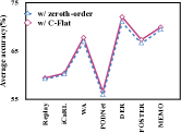
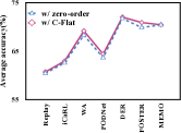
Limited work [9, 47] proved that the zeroth-order sharpness leads to flat minima boosted CL. Here, we employ a zeroth-order optimizer [19] instead of vanilla-SGD to verify the performance of C-Flat. As shown in  Fig. 2, C-Flat (purple line) stably outperforms the zeroth-order sharpness (blue line) on all baselines. We empirically demonstrated that flatter is better for continual learning.

Former work FS-DGPM [9] regulates the gradient direction with flat minima to promote CL. The FS (Flattening Sharpness) term derived from FS-DGPM is a typical zeroth-order flatness. We revisit the FS-DGPM series (including La/FS-GPM, DGPM, La/FS-DGPM) [9, 44] to evaluate performance using C-Flat instead of FS (see Algorithm 2).  Table 2 yields two conclusions: (i) C-Flat boosts the GPM [44] baseline as a pluggable regularization term. This not only extends the frontiers of CL methods, incorporating gradient-based solutions, but also reaffirms the remarkable versatility of C-Flat. (ii) Throughout all series of FS-DGPM, C-Flat seamlessly supersedes FS and achieves significantly better performance. This indicates that C-Flat consistently exceeds zeroth-order sharpness. Hence, reconfirming that C-Flat is indeed a simple yet potential CL method that deserves to be widely spread within the CL community.

4.4 Visualization of Landscapes

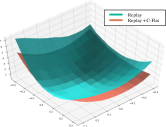
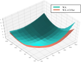
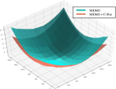
More intuitively, we present a detailed visualization of landscape. PyHessian [55] is used to draw the loss landscape of models. To simplify, we choose one typical method from each category of CL methods (Replay, Wa, MEMO) for testing.  Figure 3 clearly illustrates that, by applying C-Flat, the loss landscape becomes much flatter than that of the vanilla method. This trend consistently holds across various categories of CL methods, providing strong empirical support for C-Flat, and confirms our intuition.

(a)

(b)

(c)

(d)

Figure 4: The Hessian eigenvalues and the traces at epochs 50, and 150 on B0_Inc10 setting (MEMO, CIFAR-100) w/ and w/o C-Flat plugged in.

4.5 Hessian Eigenvalues and Hessian Traces

In this subsection, we use Hessian Eigenvalues and Hessian trace to demonstrate how is C-Flat beneficial to CL.

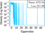
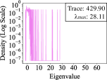
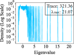
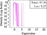
Hessian Eigenvalues.  Equation 12 delineates the connection between fist-order flatness and Hessian eigenvalues in CL. Broadly, Hessian eigenvalues serve as a metric for assessing the flatness of a function. Thus we report Hessian eigenvalue distributions in  Fig. 4 for empirical analysis. As shown in  Fig. 4, models trained with vanilla-SGD exhibit higher maximal Hessian eigenvalues (67.48/21.07 at epochs 50/150 in  Fig. 4(a) and  Fig. 4(c)), while our method induces a significant drop in Hessian eigenvalues to 28.11/6.25 at epochs 50/150 in  Fig. 4(b) and  Fig. 4(d)) during CL, leading to flatter minima. Consequently, the performance of CL is tangibly enhanced.

Hessian Traces. We calculate the empirical Fisher information matrix as an estimation of the Hessian and leverage the trace of this to quantify the flatness of the approximation loss at the convergence point. As depicted in  Fig. 4, we observe that a substantial reduction in the Hessian trace when employing our method compared with vanilla-SGD (670.36/321.36 drops to 429.90/97.36 at epochs 50/150 in  Fig. 4(b) and  Fig. 4(d)). This observation suggests that our method induces a flatter minimum. These findings not only align with but also substantiate the theoretical insights presented in the methodology section.

4.6 Computation Overhead

(a)

(b)

Figure 5: Analysis of computation overhead

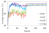
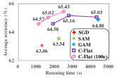
To assess the efficiency of C-Flat, we provides a thorough analysis from the convergence speed and running time with CIFAR-100/B0_Inc20 on Replay. As shown in Fig. 5, C-Flat is compared with SGD and other flatness-aware optimiziters. We train C-Flat optimizers on CL benchmarks with 20%, 50%, 100% of iterations and approximately 60% of epochs, while holding the other optimizers at 100%. Fig. LABEL:subfig:converge_seed first shows that C-Flat converges fastest and has the highest accuracy (purple line), meaning few iterations/epochs with C-Flat is enough to improve CL. Fig. LABEL:subfig:runtime_acc shows i) Compared with SGD, with only 20% of iterations and 60% of epochs (pink line) using C-Flat, CL performance is improved using slightly less time; ii) C-Flat surpasses GAM with similar time as SAM when setting the iterations/epochs ratio to 50%/60%; iii) Models trained with C-Flat for 100 epochs outperform those trained with other optimizers for 170 epochs. To sum up, we show that C-Flat outperforms current optimizers with fewer training iterations and epochs. This indicates the effectiveness and efficiency of C-Flat.

4.7 Ablation Study

(a)

(b)

(c)

(d)

Figure 6: Ablation study about $\lambda$ and $\rho$. (a) and (b) represents the effect of $\lambda$ and $\rho$ on different CL methods (WA, Replay, MEMO); (c) and (d) represents the effect of $\rho$ and $\rho$ scheduler on MEMO with different optimizers (SGD (red line), SAM, GAM).

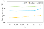
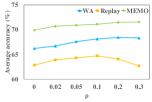
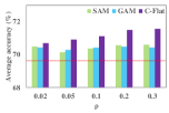
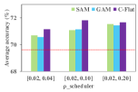
We perform ablation study in two cases: (i) the influence of $\lambda$ and $\rho$ on different CL methods; (ii) the influence of $\rho$ and its scheduler on different optimizers.

How $\lambda$ and $\rho$ affects various CL methods? We first present the performance of C-Flat with varying $\lambda$ and $\rho$. As described in Eq. 13, $\lambda$ controls the strength of the C-Flat penalty (when $\lambda$ is equal to 0, this means that first-order flatness is not implemented). As shown in  LABEL:subfig:param_lambda_CL, compared with vanilla optimizer, C-Flat shows remarkable improvement with varying $\lambda$. Moreover, $\rho$ controls the step length of gradient ascent. As shown in  LABEL:subfig:param_rho_CL, C-Flat with $\rho$ larger than 0 outperforms C-Flat without gradient ascent, showing that C-Flat benefits from the gradient ascent.

$\rho$ and $\rho$ scheduler on flat sharpness optimizers. For each CL task $T$, same learning rate $\eta^{T}$ and neighborhood size $\rho^{T}$ initialization are used. By default, $\rho^{T}_{i}\in[\rho_{\_},\rho_{+}]$ is set as a constant, which decays with respect to the learning rate $\eta^{T}_{i}\in[\eta_{\_},\eta_{+}]$ by $\rho^{T}_{i}=\rho_{\_}+\frac{(\rho_{+}-\rho_{\_})}{\eta_{+}-\eta_{\_}}(\eta^{T}_{i}-\eta_{\_})$.  LABEL:subfig:param_rho_optim and  LABEL:subfig:param_rho_sche present a comparison on $\rho$ initialization and $\{\rho_{\_},\rho_{+}\}$ scheduler. C-Flat outperforms across various settings, and is not oversensitive to hyperparameters in a reasonable range.

4.8 Beyond Not-forgetting

Table 3: Analysis of BT and FT. RR refers to Relative Return on w/o and w/ C-Flat.

Method		CIFAR-100/ B0_Inc5
		w/o C-Flat	w/ C-Flat	RR
iCaRL [41]	old	36.36	37.12	BT+2.10%
	new	80.25	82.20	FT+2.43%
PODNet [10]	old	46.32	47.44	BT+2.42%
	new	62.65	64.75	FT+3.35%
FOSTER [51]	old	58.50	61.35	BT+2.85%
	new	62.05	63.05	FT+1.61%

As is known to all, forward, and in particular backward transfer, are the desirable conditions for CL [22]. Here, we thoroughly examine the performance of C-Flat in both aspects. Forward Transfer (FT) means better performance on each subsequent task. Backward Transfer (BT) means better performance on previous tasks, when revisited. We count the performance of new and old tasks on several CL benchmarks before and after using C-Flat. As observed in  Tab. 3, C-Flat consistently improves the learning performance of both new and old tasks. This observation indicates that C-Flat empowers these baselines with robust forward and backward transfer capabilities, that is learning a task should improve related tasks, both past and future. But, thus far, achieving a baseline that maintains perfect recall (by forgetting nothing) remains elusive. Should such a baseline emerge, C-Flat stands poised to empower it with potent backward transfer, potentially transcending the limitations of mere not-forgetting.

5 Conclusion

This paper presents a versatile optimization framework, C-Flat, to confront forgetting. Empirical results demonstrate C-Flat’s consistently outperform on all sorts of CL methods, showcasing its plug-and-play feature. Moreover, the exploration of Hessian eigenvalues and traces reaffirms the efficacy of C-Flat in inducing flatter minima to enhance CL. In essence, C-Flat emerges as a simple yet powerful addition to the CL toolkit, making continual learning stronger.

References

- [1] Abati, D., Tomczak, J., Blankevoort, T., Calderara, S., Cucchiara, R., Bejnordi, B.E.: Conditional channel gated networks for task-aware continual learning. In: CVPR (2020)
- [2] Akyürek, A.F., Akyürek, E., Wijaya, D.T., Andreas, J.: Subspace regularizers for few-shot class incremental learning. ICLR (2022)
- [3] Andriushchenko, M., Flammarion, N.: Towards understanding sharpness-aware minimization. In: ICML (2022)
- [4] Baldassi, C., Pittorino, F., Zecchina, R.: Shaping the learning landscape in neural networks around wide flat minima. Proceedings of the National Academy of Sciences 117(1), 161–170 (2020)
- [5] Bhat, P., Zonooz, B., Arani, E.: Task-aware information routing from common representation space in lifelong learning. ICLR (2023)
- [6] Cha, S., Hsu, H., Hwang, T., Calmon, F.P., Moon, T.: Cpr: classifier-projection regularization for continual learning. ICLR (2021)
- [7] Chaudhry, A., Ranzato, M., Rohrbach, M., Elhoseiny, M.: Efficient lifelong learning with a-gem. arXiv preprint arXiv:1812.00420 (2018)
- [8] Delange, M., Aljundi, R., Masana, M., Parisot, S., Jia, X., Leonardis, A., Slabaugh, G., Tuytelaars, T.: A continual learning survey: Defying forgetting in classification tasks. IEEE Transactions on Pattern Analysis and Machine Intelligence (2021)
- [9] Deng, D., Chen, G., Hao, J., Wang, Q., Heng, P.A.: Flattening sharpness for dynamic gradient projection memory benefits continual learning. NeurIPS 34 (2021)
- [10] Douillard, A., Cord, M., Ollion, C., Robert, T., Valle, E.: Podnet: Pooled outputs distillation for small-tasks incremental learning. In: ECCV (2020)
- [11] Driess, D., Xia, F., Sajjadi, M.S., Lynch, C., Chowdhery, A., Ichter, B., Wahid, A., Tompson, J., Vuong, Q., Yu, T., et al.: Palm-e: An embodied multimodal language model. arXiv preprint arXiv:2303.03378 (2023)
- [12] Du, J., Zhou, D., Feng, J., Tan, V., Zhou, J.T.: Sharpness-aware training for free. NeurIPS
- [13] Du, Y., Czarnecki, W.M., Jayakumar, S.M., Farajtabar, M., Pascanu, R., Lakshminarayanan, B.: Adapting auxiliary losses using gradient similarity. arXiv preprint arXiv:1812.02224 (2018)
- [14] Farajtabar, M., Azizan, N., Mott, A., Li, A.: Orthogonal gradient descent for continual learning. In: International Conference on Artificial Intelligence and Statistics. pp. 3762–3773. PMLR (2020)
- [15] Feng, T., Ji, K., Bian, A., Liu, C., Zhang, J.: Identifying players in broadcast videos using graph convolutional network. Pattern Recognition 124, 108503 (2022)
- [16] Feng, T., Wang, M., Yuan, H.: Overcoming catastrophic forgetting in incremental object detection via elastic response distillation. In: CVPR (2022)
- [17] Feng, T., Xu, L., Yuan, H., Zhao, Y., Tang, M., Wang, M.: Towards mask-robust face recognition. In: Proceedings of the IEEE/CVF International Conference on Computer Vision. pp. 1492–1496 (2021)
- [18] Feng, T., Yuan, H., Wang, M., Huang, Z., Bian, A., Zhang, J.: Progressive learning without forgetting. arXiv preprint arXiv:2211.15215 (2022)
- [19] Foret, P., Kleiner, A., Mobahi, H., Neyshabur, B.: Sharpness-aware minimization for efficiently improving generalization. arXiv preprint arXiv:2010.01412 (2020)
- [20] Foret, P., Kleiner, A., Mobahi, H., Neyshabur, B.: Sharpness-aware minimization for efficiently improving generalization. In: ICLR (2021), https://openreview.net/forum?id=6Tm1mposlrM
- [21] Gao, Q., Zhao, C., Ghanem, B., Zhang, J.: R-dfcil: Relation-guided representation learning for data-free class incremental learning. In: ECCV (2022)
- [22] Hadsell, R., Rao, D., Rusu, A.A., Pascanu, R.: Embracing change: Continual learning in deep neural networks. Trends in cognitive sciences 24(12), 1028–1040 (2020)
- [23] He, H., Huang, G., Yuan, Y.: Asymmetric valleys: Beyond sharp and flat local minima. NeurIPS 32 (2019)
- [24] Hu, Z., Li, Y., Lyu, J., Gao, D., Vasconcelos, N.: Dense network expansion for class incremental learning. In: CVPR (2023)
- [25] Jeeveswaran, K., Bhat, P., Zonooz, B., Arani, E.: Birt: Bio-inspired replay in vision transformers for continual learning. ICML (2023)
- [26] Jin, X., Sadhu, A., Du, J., Ren, X.: Gradient-based editing of memory examples for online task-free continual learning. NeurIPS (2021)
- [27] Keskar, N.S., Mudigere, D., Nocedal, J., Smelyanskiy, M., Tang, P.T.P.: On large-batch training for deep learning: Generalization gap and sharp minima. arXiv preprint arXiv:1609.04836 (2016)
- [28] Kim, D.Y., Han, D.J., Seo, J., Moon, J.: Warping the space: Weight space rotation for class-incremental few-shot learning. In: ICLR (2022)
- [29] Kirkpatrick, J., Pascanu, R., Rabinowitz, N., Veness, J., Desjardins, G., Rusu, A.A., Milan, K., Quan, J., Ramalho, T., Grabska-Barwinska, A., et al.: Overcoming catastrophic forgetting in neural networks. PNAS (2017)
- [30] Kong, Y., Liu, L., Chen, H., Kacprzyk, J., Tao, D.: Overcoming catastrophic forgetting in continual learning by exploring eigenvalues of hessian matrix. IEEE Transactions on Neural Networks and Learning Systems (2023)
- [31] Konishi, T., Kurokawa, M., Ono, C., Ke, Z., Kim, G., Liu, B.: Parameter-level soft-masking for continual learning. arXiv preprint arXiv:2306.14775 (2023)
- [32] Li, Z., Hoiem, D.: Learning without forgetting. IEEE Trans. Pattern Anal. Mach. Intell. 40(12), 2935–2947 (2018)
- [33] Lin, H., Zhang, B., Feng, S., Li, X., Ye, Y.: Pcr: Proxy-based contrastive replay for online class-incremental continual learning. In: CVPR (2023)
- [34] Lin, S., Yang, L., Fan, D., Zhang, J.: Trgp: Trust region gradient projection for continual learning. arXiv preprint arXiv:2202.02931 (2022)
- [35] Liu, H., Liu, H.: Continual learning with recursive gradient optimization. International Conference on Learning Representations (2022)
- [36] Liu, Y., Schiele, B., Sun, Q.: Adaptive aggregation networks for class-incremental learning. In: CVPR (2021)
- [37] Liu, Y., Mai, S., Chen, X., Hsieh, C.J., You, Y.: Towards efficient and scalable sharpness-aware minimization. In: CVPR (2022)
- [38] Lopez-Paz, D., Ranzato, M.: Gradient episodic memory for continual learning. NeurIPS (2017)
- [39] Masana, M., Liu, X., Twardowski, B., Menta, M., Bagdanov, A.D., Van De Weijer, J.: Class-incremental learning: survey and performance evaluation on image classification. IEEE Transactions on Pattern Analysis and Machine Intelligence (2022)
- [40] Oh, Y., Baek, D., Ham, B.: Alife: Adaptive logit regularizer and feature replay for incremental semantic segmentation. NeurIPS (2022)
- [41] Rebuffi, S.A., Kolesnikov, A., Sperl, G., Lampert, C.H.: icarl: Incremental classifier and representation learning. In: CVPR (2017)
- [42] Rolnick, D., Ahuja, A., Schwarz, J., Lillicrap, T., Wayne, G.: Experience replay for continual learning. In: NeurIPS. vol. 32 (2019)
- [43] Rudner, T.G., Smith, F.B., Feng, Q., Teh, Y.W., Gal, Y.: Continual learning via sequential function-space variational inference. In: International Conference on Machine Learning. pp. 18871–18887. PMLR (2022)
- [44] Saha, G., Garg, I., Roy, K.: Gradient projection memory for continual learning. In: International Conference on Learning Representations (2020)
- [45] Sener, O., Koltun, V.: Multi-task learning as multi-objective optimization. NeurIPS (2018)
- [46] Serrà, J., Suris, D., Miron, M., Karatzoglou, A.: Overcoming catastrophic forgetting with hard attention to the task. In: ICML. pp. 4555–4564 (2018)
- [47] Shi, G., Chen, J., Zhang, W., Zhan, L.M., Wu, X.M.: Overcoming catastrophic forgetting in incremental few-shot learning by finding flat minima. NeurIPS (2021)
- [48] Sun, W., Li, Q., Zhang, J., Wang, W., Geng, Y.a.: Decoupling learning and remembering: A bilevel memory framework with knowledge projection for task-incremental learning. In: CVPR (2023)
- [49] Sun, Z., Mu, Y., Hua, G.: Regularizing second-order influences for continual learning. In: CVPR (2023)
- [50] van de Ven, G.M., Tuytelaars, T., Tolias, A.S.: Three types of incremental learning. Nature Machine Intelligence pp. 1185–1197 (2022)
- [51] Wang, F.Y., Zhou, D.W., Ye, H.J., Zhan, D.C.: Foster: Feature boosting and compression for class-incremental learning. In: European conference on computer vision. pp. 398–414 (2022)
- [52] Wang, L., Zhang, X., Su, H., Zhu, J.: A comprehensive survey of continual learning: Theory, method and application. arXiv preprint arXiv:2302.00487 (2023)
- [53] Wang, Z., Tsvetkov, Y.: Gradient vaccine: Investigating and improving multi-task optimization in massively multilingual models. In: Proceedings of the International Conference on Learning Representations (ICLR) (2021)
- [54] Yan, S., Xie, J., He, X.: DER: dynamically expandable representation for class incremental learning. In: CVPR. pp. 3014–3023 (2021)
- [55] Yao, Z., Gholami, A., Keutzer, K., Mahoney, M.W.: Pyhessian: Neural networks through the lens of the hessian (2019), http://arxiv.org/abs/1912.07145
- [56] Yoon, J., Kim, S., Yang, E., Hwang, S.J.: Scalable and order-robust continual learning with additive parameter decomposition. In: International Conference on Learning Representations (2020)
- [57] Yuan, H., Jiang, J., Albanie, S., Feng, T., Huang, Z., Ni, D., Tang, M.: Rlip: Relational language-image pre-training for human-object interaction detection. In: NeurIPS (2022)
- [58] Yuan, H., Zhang, S., Wang, X., Albanie, S., Pan, Y., Feng, T., Jiang, J., Ni, D., Zhang, Y., Zhao, D.: Rlipv2: Fast scaling of relational language-image pre-training. In: ICCV (2023)
- [59] Yuan, H., Zhang, S., Wang, X., Wei, Y., Feng, T., Pan, Y., Zhang, Y., Liu, Z., Albanie, S., Ni, D.: Instructvideo: Instructing video diffusion models with human feedback (2024)
- [60] Zhang, X., Xu, R., Yu, H., Zou, H., Cui, P.: Gradient norm aware minimization seeks first-order flatness and improves generalization. In: CVPR 2023. pp. 20247–20257 (2023)
- [61] Zhao, B., Xiao, X., Gan, G., Zhang, B., Xia, S.T.: Maintaining discrimination and fairness in class incremental learning. In: CVPR (2020)
- [62] Zhong, Q., Ding, L., Shen, L., Mi, P., Liu, J., Du, B., Tao, D.: Improving sharpness-aware minimization with fisher mask for better generalization on language models. arXiv preprint arXiv:2210.05497 (2022)
- [63] Zhou, D.W., Wang, F.Y., Ye, H.J., Zhan, D.C.: Pycil: A python toolbox for class-incremental learning (2023)
- [64] Zhou, D.W., Wang, Q.W., Qi, Z.H., Ye, H.J., Zhan, D.C., Liu, Z.: Deep class-incremental learning: A survey. arXiv preprint arXiv:2302.03648 (2023)
- [65] Zhou, D.W., Wang, Q.W., Ye, H.J., Zhan, D.C.: A model or 603 exemplars: Towards memory-efficient class-incremental learning. ICLR (2023)
- [66] Zhu, K., Zhai, W., Cao, Y., Luo, J., Zha, Z.J.: Self-sustaining representation expansion for non-exemplar class-incremental learning. In: CVPR (2022)
- [67] Zhuang, J., Gong, B., Yuan, L., Cui, Y., Adam, H., Dvornek, N., Tatikonda, S., Duncan, J., Liu, T.: Surrogate gap minimization improves sharpness-aware training. arXiv preprint arXiv:2203.08065 (2022)
- [68] Ziemke, T.: Embodied ai as science: Models of embodied cognition, embodied models of cognition, or both? pp. 27–36 (2004)
- [69] Zinkevich, M.: Online convex programming and generalized infinitesimal gradient ascent. In: Machine Learning, Proceedings of the Twentieth International Conference (ICML) (2003)