BadPart: Unified Black-box Adversarial Patch Attacks
against Pixel-wise Regression Tasks

Abstract

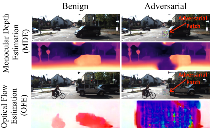
Pixel-wise regression tasks (e.g., monocular depth estimation (MDE) and optical flow estimation (OFE)) have been widely involved in our daily life in applications like autonomous driving, augmented reality and video composition. Although certain applications are security-critical or bear societal significance, the adversarial robustness of such models are not sufficiently studied, especially in the black-box scenario. In this work, we introduce the first unified black-box adversarial patch attack framework against pixel-wise regression tasks, aiming to identify the vulnerabilities of these models under query-based black-box attacks. We propose a novel square-based adversarial patch optimization framework and employ probabilistic square sampling and score-based gradient estimation techniques to generate the patch effectively and efficiently, overcoming the scalability problem of previous black-box patch attacks. Our attack prototype, named BadPart, is evaluated on both MDE and OFE tasks, utilizing a total of 7 models. BadPart surpasses 3 baseline methods in terms of both attack performance and efficiency. We also apply BadPart on the Google online service for portrait depth estimation, causing 43.5% relative distance error with 50K queries. State-of-the-art (SOTA) countermeasures cannot defend our attack effectively.

1 Introduction

Figure 1: Adversarial patch attack on pixel-wise regression tasks.

Pixel-wise regression tasks represent a family of computer vision tasks that employ images as input and generate continuous regression values for each pixel in the input image. Examples of such tasks include monocular depth estimation (MDE), optical flow estimation (OFE), surface normal estimation (SNE), among others. The evolution of deep learning techniques has led to the development of numerous DNN models that have demonstrated impressive performance on these tasks, thereby enabling a variety of downstream applications such as autonomous driving, augmented reality, video composition, and more. Given the extensive and security-sensitive nature of some of these applications, it is crucial to examine the adversarial robustness of these tasks.

Previous adversarial patch attacks on pixel-wise regression models (Cheng et al., 2022) have primarily been conducted in a white-box setting, where the attacker has complete knowledge of the target model and can use gradient-based optimization to create the patch and compromise the model. However, this white-box assumption is not always feasible. For instance, models used in autonomous driving systems are typically closed-source (Tesla, ). Moreover, some models are provided as an online service, preventing users from accessing their internals model structures (Google3DPortrait, ). In typical scenarios, black-box attacks are more realistic and could pose a greater threat to the security of these tasks. Existing black-box attack techniques are either based on training a substitute model or iteratively querying the model. In this study, we focus on the query-based approach as it reduces the cost of model training and only assumes that the attacker has access to the model output. This leads us to a pivotal inquiry: “can we craft an adversarial patch to compromise the pixel-wise regression model through iterative querying in a black-box manner?”

Answering the above question may bear direct relevance to applications of societal significance. For instance, in the realm of autonomous driving, attackers have been able to exploit the pixel-wise regression output of Tesla’s depth estimation model through hacking (Lambert, 2021), and online services, such as Google Depth API (Google3DPortrait, ) and Clipdrop API (Clipdrop, ), readily provide access to pixel-wise model outputs. The feasibility of such attacks within the context of autonomous driving would introduce a notable security concern. Meanwhile, on the other hand, the adversarial patch for online services could also act as a deterrent against unauthorized users who attempt to upload our photographs to those services for video composition.

To the best of our knowledge, we are the first to explore unified black-box patch attacks against pixel-wise regression tasks. Compared to classification tasks, pixel-wise regression tasks have denser (pixel-wise) query output and the resolution of input images is significantly higher. For example, the representative KITTI dataset (Uhrig et al., 2017) used in MDE and OFE tasks includes images with a resolution of $1242\times 375$, while most previous black-box patch attacks on classification models (Tao et al., 2023) use images from MINIST, CIFAR-10, GTSRB, etc., with a resolution less than $32\times 32$. The search space for a patch covering 1% of the input images would expand exponentially as the resolution increases, hence the effectiveness and efficiency of prior methods are limited when adapted to our scenario.

To address this issue and enhance the scalability of black-box patch generation, we leverage the domain knowledge of pixel-wise regression tasks and propose a novel square-based adversarial patch optimization framework. Specifically, in each iteration, we consider a small square area within the patch region to reduce the potential search space, then we introduce a batch of random noises on the square area to estimate the gradients of the region by evaluating the score of each noise in terms of attack performance. We sample the location of the square area probabilistically based on the pixel-wise error distribution, and propose novel score adjustment procedures for more precise gradient estimation. The source code is available. Figure 1 presents our attack performance. In summary, our contributions are as follows:

• We introduce the first unified black-box adversarial patch attack framework against pixel-wise regression tasks (e.g., monocular depth estimation and optical flow estimation).

• We devise a square-based universal adversarial patch generation approach, employing probabilistic square sampling and score-based gradient estimation, to facilitate scalable black-box patch optimization.

• We implement an attack prototype called BadPart (Black-box adversarial patch attack against pixel-wise regression tasks). We evaluate the attack performance of BadPart on both MDE and OFE tasks, utilizing a total of 7 models that encompass both popular and SOTA ones. Compared with three baseline methods that employ varying black-box optimization strategies, BadPart surpasses them in terms of both attack performance and efficiency. We also apply BadPart to attack a Google online service for portrait depth estimation (Google3DPortrait, ), resulting in 43.5% relative distance error with 50K queries.

2 Background and Related Work

Pixel-wise Regression Tasks. Pixel-wise regression tasks generate continuous values for each input pixel, differing from pixel-wise classification tasks like semantic segmentation (Yu et al., 2018; Zhou et al., 2022), which assign a discrete class label to every pixel. Representative tasks of this type include monocular depth estimation (MDE) (Moon et al., 2019; Watson et al., 2019; Wang et al., 2023a), optical flow estimation (OFE) (Teed & Deng, 2020; Ilg et al., 2017; Dosovitskiy et al., 2015), and surface normal estimation (SNE) (Zeng et al., 2019; Lenssen et al., 2020; Bae et al., 2021). In MDE models, the output comprises the estimated pixel-wise distance between the 3D scenario and the camera capturing the input image, with each pixel corresponding to a distance estimation. OFE models use two consecutive image frames as input and output the estimated motion of pixels (the “optical flow”) between the two frames. For each pixel in the first frame, a 2D vector is estimated, indicating its offset to the corresponding pixel in the second frame. SNE models output the estimated orientations of the surfaces in the input image, described with the ”normal vectors” in 3D space that are perpendicular to the surface at the locations of pixels. Given that the first two tasks (MDE and OFE) have broader and more security-critical applications, such as autonomous driving (Karpathy, 2020), visual SLAM (Wimbauer et al., 2021), video composition (Liew et al., 2023), and augmented reality (Bang et al., 2017), our discussion primarily focuses on these two tasks. However, our proposed attack is a unified approach and can be readily applied to other pixel-wise regression tasks like SNE.

Black-box Adversarial Attacks. Existing black-box attacks can be broadly classified into two categories: substitute model-based attacks and query-based attacks. In the former, attackers construct a substitute model to execute white-box attacks and transfer the generated adversarial example to attack the victim model  (Gao et al., 2020; Liu et al., 2016; He et al., 2021). To construct the substitute model, attackers employ the same training set as the victim model or reverse-engineer/synthesize a similar dataset. Many works propose innovative training approaches to further improve the transferability (Wu et al., 2020; Feng et al., 2022; Wang & He, 2021; Wang et al., 2021). In the latter category of attacks, known as query-based attacks, attackers directly optimize the adversarial example by iteratively querying the victim model. Most black-box attacks focus on classification tasks, and they can be further divided into two groups: hard-label attacks and soft-label attacks, depending on the query output that the attacker can access. Hard-label attacks (Chen et al., 2020; Li et al., 2020; Yan et al., 2020; Tao et al., 2023) assume that the attacker can only access the predicted label of the victim model, while soft-label attacks (Croce et al., 2022; Ilyas et al., 2018; Moon et al., 2019) assume the prediction score of each class is available. With iterative queries, some prior works optimize the adversarial noise via gradient estimation (Chen et al., 2019; Zhang et al., 2021; Tao et al., 2023), and some others rely on heuristic random search (Croce et al., 2022; Andriushchenko et al., 2020; Duan et al., 2021). Additionally, there are studies utilizing genetic algorithms to optimize the noise (Ilie et al., 2021; Alzantot et al., 2019). Our work also falls under the category of query-based black-box attacks. However, we are the first to target pixel-wise regression tasks. We confront the domain-specific obstacle of high-resolution patch optimization, given that the SOTA black-box patch attack (Tao et al., 2023) primarily concentrates on smaller patches and exhibits limited scalability in our scenario.

3 Problem Formalization

The objective of the attack is to generate an adversarial patch, denoted as $\mathbf{p}$, for a black-box pixel-wise regression model $\mathcal{M}$. The desired result is that, irrespective of the input image $\mathbf{x}$, the attachment of the patch at location $\mathbf{q}$ on $\mathbf{x}$ will substantially degrade the model performance. Attackers can only query $\mathcal{M}$ for pixel-wise output. This black-box setting is highly practical as there are online services (Google3DPortrait, ; Clipdrop, ) that only allow users to upload custom images via API and return the depth estimation result. Additionally, in autonomous driving, attackers have shown to be able to reverse-engineer Tesla Autopilot to access the estimated depth map (Lambert, 2021). Formally, the optimization problem is expressed as follows:

$$\max\limits_{\mathbf{p}}~{} Mean\left(\mathcal{F}\left(\mathcal{M}([\mathbf{x^{\prime}}]_{n})-\mathcal{M}([\mathbf{x_{0}^{\prime}}]_{n})\right)\right)$$ (1)

s.t. $$\mathbf{p}\in[0,1]^{3\times h\times h},$$ (2)

where $$[\mathbf{x^{\prime}}]_{n}=\Lambda([\mathbf{x}]_{n},\mathbf{p},\mathbf{q}),$$ (3)

$$[\mathbf{x_{0}^{\prime}}]_{n}=\Lambda([\mathbf{x}]_{n},\mathbf{p_{0}},\mathbf{q}),$$ (4)

$$\mathcal{F}:\mathbb{R}^{n\times d\times H\times W}\rightarrow\mathbb{R}^{H\times W}$$ (5)

$$\mathbf{x}\in[0,1]^{3\times H\times W},~{}\mathbf{p}_{0}=\{0\}^{3\times h\times h},$$ (6)

$$\mathbf{q}\in\{(i,j)|i=\frac{h}{2}...H_{\!}-_{\!}\frac{h}{2},j=\frac{h}{2}...W_{\!}-_{\!}\frac{h}{2}\}.$$ (7)

Here, $H$ and $W$ denote the height and width of the input image $\mathbf{x}$, $h$ the size of the patch $\mathbf{p}$, $n$ the number of images in the test set and $\mathbf{q}$ the coordinates of the patch’s center in $\mathbf{x}$. We use $\Lambda(\mathbf{a_{1}},\mathbf{a_{2}},\mathbf{a_{3}})$ to denote the process of attaching $\mathbf{a_{2}}$ to $\mathbf{a_{1}}$ at location $\mathbf{a_{3}}$, hence $[\mathbf{x^{\prime}}]_{n}$ in Equation 3 refers to the image set attached with adversarial patch $\mathbf{p}$ at location $\mathbf{q}$, and $[\mathbf{x_{0}^{\prime}}]_{n}$ in Equation 4 denotes the corresponding images attached with a black patch $\mathbf{p}_{0}$ (not optimized) as reference. The output of model $\mathcal{M}$ has a dimension of $n\times d\times H\times W$, where $d$ refers to the output channels for each image. For MDE models $d$ equals 1 as the output is the estimated distance for each pixel, and for OFE models $d$ equals 2 since the model outputs the estimated pixel-wise offset vector (two dimensions). $\mathcal{F}$ in Equation 5 denotes the function calculating the pixel-wise prediction error caused by the generated adversarial perturbation.

$$\mathcal{F}(\mathbf{D})[i,j] =Mean(\{\mathbf{\mathbf{D}}[k,1,i,j]~{}|~{}k=1...n\})$$ (8)

$$\mathcal{F}(\mathbf{D})[i,j] =Mean(\{\|\mathbf{D}[k,:,i,j]\|_{2}~{}|~{}k=1...n\})$$ (9)

Our attack goals are to maximize the estimated pixel-wise distances for MDE models or the $l_{2}$ norm of offset vectors for OFE models, hence, let $\mathbf{D}=\mathcal{M}([\mathbf{x^{\prime}}]_{n})-\mathcal{M}([\mathbf{x_{0}^{\prime}}]_{n})$, $\mathcal{F}$ is defined in Equation 8 for MDE models and in Equation 9 for OFE models. For simplicity, see Equation 10, we use $\mathcal{F}_{e}([\mathbf{x^{\prime}}]_{n})\in\mathrm{R}^{H\times W}$ to denote the pixel-wise error caused by adversarial images $[\mathbf{x^{\prime}}]_{n}$ in the following text.

$$\mathcal{F}_{e}([\mathbf{x^{\prime}}]_{n})\equiv\mathcal{F}\left(\mathcal{M}([\mathbf{x^{\prime}}]_{n})-\mathcal{M}([\mathbf{x_{0}^{\prime}}]_{n})\right)$$ (10)

4 Methods

In this section, we first introduce our proposed square-based adversarial patch generation framework, as detailed in §4.1 and explicated in Alg. 1. We then examine the two main components of the framework: the probabilistic square sampling, which is elucidated in §4.2 and Alg. 2, and the score-based gradient estimation, presented in §4.3 and Alg. 3.

Figure 2: Overview of BadPart.

4.1 Square-based Patch Generation Framework

The principal concept underlying our approach involves the iterative optimization of a square-shaped sub-area in the patch region, while altering the location and size of the target square area dynamically. Figure 2 illustrates the overview of the attack framework. The rectangles in teal ($\mathbf{p}^{(i)}$) on the left of Figure 2 denote the patch region at different optimization stages, and the small squares in orange ($\mathbf{s}_{i}$) refer to the sampled sub-areas to optimize. Steps ❶, ❼ and ❽ denote the selection of the square areas, and steps ❷-❻ present the procedure of optimizing a selected square. These selection and optimization are carried out alternately. The strategy of selecting a square area within the broader patch region serves to effectively constrain the large search space inherent to the entire patch. It is inspired from SquareAttack (Andriushchenko et al., 2020) which attacks classification models via random search and leverages square areas as the perturbation units.${}_{\!}$ The${}_{\!}$ rationale${}_{\!}$ for${}_{\!}$ favoring${}_{\!}$ a${}_{\!}$ square${}_{\!}$ shape${}_{\!}$ is${}_{\!}$ that${}_{\!}$ modern${}_{\!}$ image-processing${}_{\!}$ models${}_{\!}$ predominantly${}_{\!}$ utilize${}_{\!}$ convolutional${}_{\!}$ layers${}_{\!}$ for${}_{\!}$ feature${}_{\!}$ extraction.${}_{\!}$ The${}_{\!}$ filter${}_{\!}$ kernels${}_{\!}$ within${}_{\!}$ these${}_{\!}$ layers${}_{\!}$ are${}_{\!}$ inherently${}_{\!}$ square-shaped,${}_{\!}$ thereby${}_{\!}$ making${}_{\!}$ the${}_{\!}$ square${}_{\!}$ setting${}_{\!}$ as${}_{\!}$ the${}_{\!}$ most${}_{\!}$ efficient  (Andriushchenko et al., 2020). Unlike SquareAttack, BadPart iteratively updates each square area using novel gradient estimation rather than a single-step trial. This refinement transforms our approach into a more precise optimization process rather than random search, thereby strengthening the attack’s effectiveness. Furthermore, we focus on pixel-wise regression tasks and utilize the domain knowledge of pixel error distribution to probabilistically select square locations, significantly boosting the efficiency.

Alg. 1 describes the proposed universal adversarial patch generation framework. To begin with, we initialize the patch region with vertical strips, where the color of each stripe is sampled uniformly at random from $\{0,1\}^{3}$ (see $\mathbf{p}^{(0)}$ in Figure 2 and line 4 in Alg. 1). Then we attach the patch to the validation images at location $\mathbf{q}$, and record the overall error $\omega^{*}$ as the initialized best attack performance caused by the perturbations (lines 5-6). After initialization, we start the iterations of square sampling. In each iteration, we first calculate the pixel-wise error map $\mathbf{M}$ caused by the latest patch on validation images (lines 9-10), then, in lines 11-12, we call the probabilistic square sampling algorithm (Alg. 2 explained in §4.2) with $\mathbf{M}$ and the iteration index as input, getting the sampled square area (step ❶ in Figure 2). Next, we start optimizing the square area. In each round of optimization, we first estimate the gradients of the square area on a random training image (lines 15-16). Details of the score-based gradient estimation (steps ❷-❺ in Figure 2) will be explained in §4.3 and Alg. 3. Then we update the square area with Adam optimizer using the estimated gradients (step ❻), and evaluate the attack performance $\omega$ of the latest patch (lines 17-19). We update the best performance $\omega^{*}$ to $\omega$ if $\omega$ is better and continue the next step of optimization on this square. If the best performance is not updated for $T_{1}$ steps, which indicates this square is sufficiently explored, we stop optimizing this square and continue the${}_{\!}$ next${}_{\!}$ iteration${}_{\!}$ of${}_{\!}$ square${}_{\!}$ sampling${}_{\!}$ and${}_{\!}$ optimization${}_{\!}$ (lines${}_{\!}$ 20-21).${}_{\!}$ Line${}_{\!}$ 7${}_{\!}$ and${}_{\!}$ 23${}_{\!}$ are${}_{\!}$ noise${}_{\!}$ bound-related,${}_{\!}$ which${}_{\!}$ will${}_{\!}$ be${}_{\!}$ explained${}_{\!}$ in${}_{\!}$ §4.3.

Algorithm 1 Square-based patch generation framework

1:  Input: Pixel-wise Error Function $\mathcal{F}_{e}$, Training Images $[\mathbf{x^{t}}]_{m}$, Validation Images $[\mathbf{x^{v}}]_{n}$, Patch Location $\mathbf{q}$, Patch Size $h$.

2:  Output: The generated patch $\mathbf{p}$.

3:  function BadPart($\mathcal{F}_{e}$, $[\mathbf{x^{t}}]_{m}$, $[\mathbf{x^{v}}]_{n}$, $\mathbf{q}$, $h$) 

4:     $\mathbf{p}$ $\leftarrow$ Initialize a patch $\mathbf{p}\in[0,1]^{3\times h\times h}$ with vertical strips.

5:     $[\mathbf{x^{\prime v}}]_{n}\leftarrow\Lambda([\mathbf{x^{v}}]_{n},\mathbf{p},\mathbf{q})$ { $\rhd$ Attach patch $\mathbf{p}$ to $[\mathbf{x^{v}}]_{n}$}

6:     $\omega^{*}\leftarrow Mean(\mathcal{F}_{e}([\mathbf{x^{\prime v}}]_{n}))$ { $\rhd$ Record largest error as $\omega^{*}$}

7:     $\epsilon\leftarrow\alpha$ { $\rhd$ Initialize noise bound $\epsilon$ as $\alpha$}

8:     for $iter$ in $0...max\_iters$ do

9:        $[\mathbf{x^{\prime v}}]_{n}\leftarrow\Lambda([\mathbf{x^{v}}]_{n},\mathbf{p},\mathbf{q})$

10:        $\mathbf{M}\leftarrow\mathcal{F}_{e}([\mathbf{x^{\prime v}}]_{n})$

11:        $\mathbf{z},e\leftarrow\textsc{GetSquareArea}(iter,\mathbf{M},\mathbf{q},h)$ { $\rhd$ Alg. 2}

12:        $\mathbf{s}\leftarrow\mathbf{p}\left[\mathbf{z}_{c}-\frac{e}{2}...\mathbf{z}_{c}+\frac{e}{2},~{}~{}\mathbf{z}_{r}-\frac{e}{2}...\mathbf{z}_{r}+\frac{e}{2}\right]$

13:        /*** Optimize the square area ***/

14:        for $step$ in $0...max\_steps$ do

15:           $\mathbf{x}\leftarrow$ Randomly sample an image from $[\mathbf{x^{t}}]_{m}$.

16:           $\mathbf{g}\leftarrow\textsc{GetGrad}(\mathcal{F}_{e},\mathbf{x},\mathbf{p},\mathbf{q},\mathbf{z},e,\epsilon)$ { $\rhd$ Alg. 3}

17:           $\mathbf{s}\leftarrow Optimizer(\mathbf{s},\mathbf{g})$

18:           $\mathbf{p}\leftarrow\Lambda(\mathbf{p},\mathbf{s},\mathbf{z})$ { $\rhd$ Attach $\mathbf{s}$ to $\mathbf{p}$ at location $\mathbf{z}$}

19:           $\omega\leftarrow Mean\left(\mathcal{F}_{e}\left(\Lambda\left([\mathbf{x^{v}}]_{n},\mathbf{p},\mathbf{q}\right)\right)\right)$

20:           if $\omega>\omega^{*}$ then $\omega^{*}\leftarrow\omega$;

21:           if $\omega^{*}$ is not updated for $T_{1}$ steps then break loop;

22:        end for

23:        if $\omega^{*}$ is not updated for $T_{2}$ iterations then $\epsilon\leftarrow\epsilon*\gamma$;

24:     end for

25:  end function

4.2 Probabilistic Square Sampling

The sampling algorithm is designed to enhance the probability of selecting locations within the patch region that are more vulnerable to adversarial perturbations. As indicated in (Cheng et al., 2022) and (Cheng et al., 2023), the identification of vulnerable areas on images is critical for improving attack performance. To ascertain these vulnerable areas in the beginning, we employ an initialization phase ($K$ iterations), wherein we randomly sample the square location in a uniform manner. This period is denoted as $\mathbf{p^{(1)}}$ in Figure 2. After the initialization phase, the pixel-wise error map $\mathbf{M}$ caused by the latest patch is utilized as an indication of the vulnerable areas and we leverage this map to calculate the probability distribution of location sampling. Those areas with larger errors obtain higher probability. The background color of the patch $\mathbf{p^{(1)}},\mathbf{p^{(2)}}$ and $\mathbf{p^{(3)}}$ in Figure 2 illustrate the sampling probability distribution of square locations.

Alg. 2 describes the probabilistic square area sampling algorithm, whose output are the sampled square location in the patch region and the square size. In accordance with SquareAttack, the square size is obtained from a predefined schedule regarding the iteration index (line 4), which is detailed in Appendix A. As the index escalates, the size diminishes, indicative of a transition from coarse to fine-grained optimization (see $\mathbf{s_{3}}$ after step ❽ in Figure 2). The initialization phase of uniformly sampling lasts $K$ iterations (lines 5-6), after which we start error-based probabilistic sampling. We first smooth the pixel-wise error map $\mathbf{M}$ with a filter kernel that has the same size of the square, which is to avoid extreme values at certain locations (line 9). Then we crop out the patch region and normalize the smoothed error map to $[0,1]$ followed by applying the softmax function to transform the error map into the sampling probabilities for different locations (lines 10-11). At last, see step ❼ or ❽ in Figure 2, the square location ($\mathbf{s_{2}}$ or $\mathbf{s_{3}}$) is sampled based on the probability distribution (line 12).

Algorithm 2 Probabilistic square area sampling

1:  Input: Iteration Index $iter$, Pixel-wise Error Map $\mathbf{M}$, Patch Location $\mathbf{q}$, Patch Size $h$.

2:  Output: Square Location $\mathbf{z}$, Square Size $e$.

3:  function  $\textsc{GetSquareArea}(iter,\mathbf{M},\mathbf{q},h)$ 

4:     $e\leftarrow SizeSche(iter)$ { $\rhd$ Use a pre-defined size schedule}

5:     if $iter\leq$ Initialization period $K$ then

6:        $\mathbf{z}\leftarrow$ Sample a location index from $\{0...h\}^{2}$ uniformly.

7:     else

8:        /*** Error-based probabilistic sampling ***/

9:        $\mathbf{M}\leftarrow$ Smooth error map $\mathbf{M}$ with kernel size $e\times e$.

10:        $\mathbf{M}_{\mathbf{q},h}\leftarrow\mathbf{M}\left[\mathbf{q}_{c}-\frac{h}{2}...\mathbf{q}_{c}+\frac{h}{2},~{}~{}\mathbf{q}_{r}-\frac{h}{2}...\mathbf{q}_{r}+\frac{h}{2}\right]$

11:        $\mathbf{prob}\leftarrow Softmax(\mathbf{M}_{\mathbf{q},h}/Max(\mathbf{M}_{\mathbf{q},h}))$

12:        $\mathbf{z}\leftarrow$ Sample a location index from $\{0...h\}^{2}$ with the          probability distribution $\mathbf{prob}$.

13:     end if

14:  end function

4.3 Score-based Gradient Estimation

In this section, we introduce the score-based square-area gradient estimation method. As shown on the right side of Figure 2, upon determination of the square area, we proceed to generate a batch of noise $[\bm{\delta}]_{b}$ within the confines of the square. This noise is constrained by a small threshold $\epsilon$, thereby facilitating the exploration of the adjacent high-dimensional space. Compared with the zeroth order optimization (Chen et al., 2017) that estimates the gradient pixel by pixel, our method is more efficient as the unit of gradient estimation is a square area. Values of the noise tensor are either $\epsilon$ or $-\epsilon$ as (Moon et al., 2019) has indicated that the optimal adversarial noise is mostly found on vertices of the bound. Subsequently, for each instance of noise, we utilize the alteration in attack performance, consequent to the application of the noise on the current square area, as the evaluative score $\Delta$ of the noise (see step ❷. Negative scores denote negative impact on attack performance). Since the scores could be very small and imbalanced among the positive and negative ones, we normalize the positive and negative scores by scaling them to [0,1] and [0,-1] respectively (step ❸). Next, we conduct adaptive scaling to allocate greater weights to the side (positive or negative) with fewer elements (step ❹). This procedure is inspired from (Tao et al., 2023), which subtracts the mean score from the positive and negative indicators. However, in our scenario of regression tasks, subtracting the mean score could potentially change the sign of scores, hence we opt to divide the positive (or negative) scores by the number of positive (or negative) elements for scaling purpose. Subsequently, we compute the weighted average of $[\mathbf{\delta}]_{b}$ by employing the scaled scores $[\Delta]_{b}$, followed by normalizing the output through dividing it by its $l_{2}$-norm. This procedure yields the estimated gradients (step ❺).

Details of the algorithm can be found in Alg. 3. Lines 4-5 attach the latest patch onto the input image, and crop out the square area, where $\mathbf{z}_{c}$ and $\mathbf{z_{r}}$ denote the column and row index of the square center within the patch. Lines 7-9 generate the set of random noise, and apply them to the square area, creating candidate input images $[\hat{\mathbf{x}}]_{b}$. Lines 10-13 calculate the scores $[\Delta]_{b}$ by comparing the attack performance of $[\hat{\mathbf{x}}]_{b}$ with the reference one $\mathbf{x^{\prime}}$. Subsequently, Lines 15-16 adjust the scores by normalization and adaptive scaling, and Lines 17-18 conduct the weighted average and normalization operations, achieving the final gradients. Note that, as shown in line 7 and 23 of Alg. 1, the threshold $\epsilon$ of the noise is initialized as $\alpha$ and will decay if the best attack performance $\omega^{*}$ is not updated for $T_{2}$ iterations of square selection. The decay factor $\gamma$ is set to 0.98 in our experiments.

Algorithm 3 Score-based square-area gradient estimation

1:  Input: Pixel-wise Error Function $\mathcal{F}_{e}$, Image $\mathbf{x}$, Patch $\mathbf{p}$, Patch Location $\mathbf{q}$, Square Location $\mathbf{z}$, Square Size $e$, Noise Bound $\epsilon$.

2:  Output: Estimated Gradient $\mathbf{g}$.

3:  function  $\textsc{GetGrad}(\mathcal{F}_{e},\mathbf{x},\mathbf{p},\mathbf{q},\mathbf{z},e,\epsilon)$ 

4:     $\mathbf{x^{\prime}}\leftarrow\Lambda(\mathbf{x},\mathbf{p},\mathbf{q})$ { $\rhd$ Get image with current patch attached}

5:     $\mathbf{s}\leftarrow\mathbf{p}\left[\mathbf{z}_{c}-\frac{e}{2}...\mathbf{z}_{c}+\frac{e}{2},~{}~{}\mathbf{z}_{r}-\frac{e}{2}...\mathbf{z}_{r}+\frac{e}{2}\right]$

6:     /*** Calculate noise scores ***/

7:     $[\bm{\delta}]_{b}\leftarrow$ Generate $b$ random noise $\bm{\delta}\in\{-\epsilon,\epsilon\}^{3\times e\times e}$.

8:     $[\hat{\mathbf{p}}]_{b}\leftarrow\Lambda(\mathbf{p},\mathbf{s}+[\bm{\delta}]_{b},\mathbf{z})$ { $\rhd$ Add $[\bm{\delta}]_{b}$ to $\mathbf{s}$ and attach to $\mathbf{p}$}

9:     $[\hat{\mathbf{x}}]_{b}\leftarrow\Lambda(\mathbf{x},[\hat{\mathbf{p}}]_{b},\mathbf{q})$ { $\rhd$ Get images with noise set applied}

10:     $[\Delta]_{b}\leftarrow 0$ { $\rhd$ Initialize score for each noise}

11:     for $\mathbf{\hat{x}_{i}}$ in $[\hat{\mathbf{x}}]_{b}$  do

12:        $\Delta_{i}\leftarrow Mean(\mathcal{F}_{e}(\mathbf{\hat{x}_{i}}))-Mean(\mathcal{F}_{e}(\mathbf{x^{\prime}}))$

13:     end for{ $\rhd$ Update $[\Delta]_{b}$}

14:     /*** Score Adjustment ***/

15:     $[\Delta]^{+}\leftarrow[\Delta]^{+}/Max([\Delta]^{+})$;   $[\Delta]^{-}\leftarrow[\Delta]^{-}/|Min([\Delta]^{-})|$

16:     $[\Delta]^{+}\leftarrow[\Delta]^{+}/\#([\Delta]^{+})$;   $[\Delta]^{-}\leftarrow[\Delta]^{-}/\#([\Delta]^{-})$

17:     $\mathbf{g}\leftarrow$ Weighted sum of noise $[\bm{\delta}]_{b}$ using weights $[\Delta]_{b}$.

18:     $\mathbf{g}\leftarrow\sqrt{3\cdot e\cdot e}\cdot\mathbf{g}/\|\mathbf{g}\|_{2}$ { $\rhd$ Return estimated gradient}

19:  end function

5 Evaluation

In this section, we evaluate BadPart on 2 kinds of tasks including 7 subject models. We compare with 3 baseline black-box attack methods and a white-box one. A set of ablation studies are discussed and the source code is provided.

5.1 Experiment Setup

Table 1: The mean error (depth estimation error (DEE, unit: meters) for MDE models and end point error (EPE, unit: pixels) for OFE models) caused by BadPart and other baseline methods on different target models. Larger values denote better attack performance.

	57 $\times$ 57 Patch (1%)					80 $\times$ 80 Patch (2%)					100 $\times$ 100 Patch (3%)
Models	GA	HB	S-RS	Ours	WB	GA	HB	S-RS	Ours	WB	GA	HB	S-RS	Ours	WB
Monodepth2	0.05	7.76	56.83	79.29	89.23	0.01	19.64	78.47	89.75	90.99	0.61	18.03	89.02	91.11	91.38
DepthHints	0.30	2.25	21.21	71.14	89.47	0.76	3.92	55.34	70.38	90.15	1.43	2.24	76.85	87.32	90.81
SQLDepth	0.03	0.06	28.63	48.74	55.09	0.43	0.16	39.89	54.14	61.05	0.30	0.45	48.66	54.51	61.91
PlaneDepth	0.61	0.83	4.07	48.22	90.11	1.71	1.07	7.67	46.85	90.24	1.84	1.47	26.58	80.07	82.62
FlowNetC	5.42	4.21	5.32	583.20	2403.32	4.08	3.55	447.60	1212.13	3585.12	5.15	4.43	640.30	1033.21	2345.54
FlowNet2	2.24	12.30	2.64	30.72	55.81	1.65	7.31	1.77	32.42	725.30	1.27	10.39	5.94	27.82	194.40
PWC-Net	1.93	2.04	2.35	4.87	53.68	1.73	1.90	1.66	5.26	149.30	1.48	1.53	1.44	5.32	55.31

• * Bold texts denote the best attack performance among black-box methods. Abbreviations. GA: GenAttack (Alzantot et al., 2019), HB: HardBeat (Tao et al., 2023), S-RS: Sparse-RS (Croce et al., 2022), WB: White-box Attack for reference.

Figure 3: Examples of the qualitative attack performance of BadPart and the baselines.

Tasks & Models. We evaluate BadPart on two pixel-wise regression tasks of MDE and OFE. For MDE, we use Monodepth2 (Godard et al., 2019), DepthHints (Watson et al., 2019), SQLDepth (Wang et al., 2023b) and PlaneDepth (Wang et al., 2023a) as the target models. For OFE, we attack FlowNetC (Dosovitskiy et al., 2015), FlowNet2 (Ilg et al., 2017) and PWC-Net (Sun et al., 2018). These models are selected since they cover both the popular and SOTA models, and we attack the publicly available models with the highest input resolutions from their official repositories. MDE models were trained on the KITTI depth prediction dataset (Uhrig et al., 2017) and OFE models were trained on the KITTI flow 2015 (Menze et al., 2015).

(a) Depthhints

(b) Planedepth

(c) FlowNetC

(d) FlowNet2

Figure 4: Comparison of query efficiency between BadPart and the baseline methods on four models (2% patch).

Baselines & Metrics. There are no direct baselines available due to a lack of previous research on black-box attacks against pixel-wise regression tasks. Hence we adapt three black-box patch attacks on image classification to our scenario as baselines. These include Sparse-RS (Croce et al., 2022), a soft-label attack that employs random search and is akin to the patch-attack variant of SquareAttack (Andriushchenko et al., 2020); HardBeat (Tao et al., 2023), a SOTA hard-label attack that estimates gradients; and GenAttack (Alzantot et al., 2019), a conventional approach using genetic algorithms. We also compare BadPart with the white-box attack as reference. We employ the mean depth estimation error (DEE, unit: meters) for MDE models and the mean end point error (EPE, unit: pixels) for OFE models as metrics to denote attack performance (the higher the better), which are aligned with the metrics used in prior white-box attacks on the two tasks (Cheng et al., 2022; Ranjan et al., 2019). They are calculated on the patched area and reflect the error caused by the generated adversarial noise.

Attack Settings. We use 100 scenes from KITTI flow dataset as our training set and another 5 scenes as the validation set during patch generation. (i.e., $m$ equals 100 and $n$ equals 5 in Alg. 1.) We evaluate the attack performance on a test set with 100 new scenes from the dataset, which covers different driving conditions (e.g., various road types, weathers and lighting). Each scene has two consecutive image frames since two images are required for the input of OFE models. For MDE models, we only feed the first frame. Detailed attack settings can be found in Appendix A, including hyper-parameter settings, devices, runtime overhead, etc.

5.2 Attack Performance

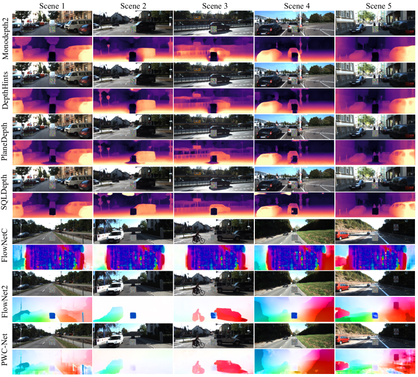
We compare the attack performance of BadPart with other baseline methods. We report the maximum attack performance of each method until convergence or after 1000K queries, whichever first. We also include the performance of white-box attacks as references. Three different patch sizes are evaluated and the patch locates at the center of the image. Table 1 reports the result. The first column denotes various pixel-wise regression models under attack, and the following columns represent attack performance of different methods and the white-box reference. As shown, BadPart obtains the best attack performance on all models under various patch sizes. The performance of BadPart is even close to the white-box attack reference on some models (e.g., Monodepth2, DepthHints and SQLDepth). Sparse-RS has the second best attack performance while GenAttack performs the worse and has nearly no effect. Figure 3 presents qualitative examples of the attack performance of different methods on PlaneDepth and FlowNetC. As shown, the first column denotes the benign scene and the MDE and OFE output. The following columns show the $2\%$ adversarial patches generated by BadPart and baseline methods, as well as the model output. In the first row, when the patch generated by BadPart is applied, the depth estimation of the patched area is significantly further than the actual distance (darker color denotes further distance estimation). In comparison, the patches generated by other methods cause less impact. In the second row, patches generated by BadPart and Sparse-RS have degraded the OFE performance significantly, making the result unusable. More qualitative and quantitative results are in Appendix C.

5.3 Query Efficiency

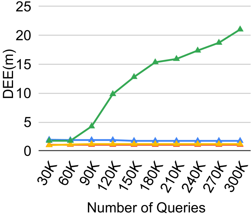
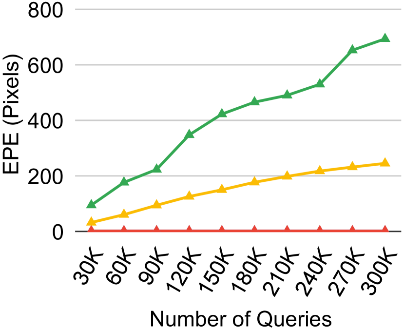
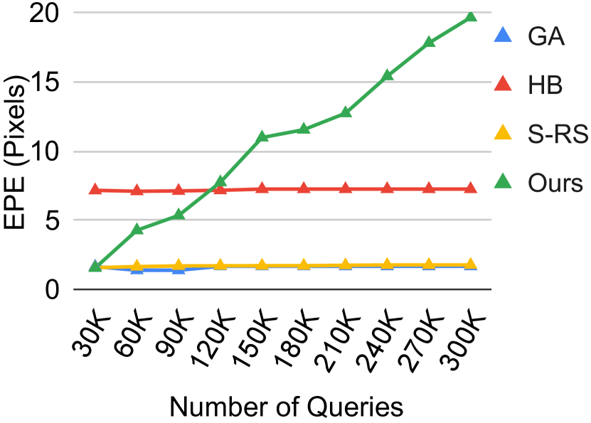
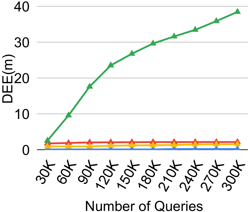
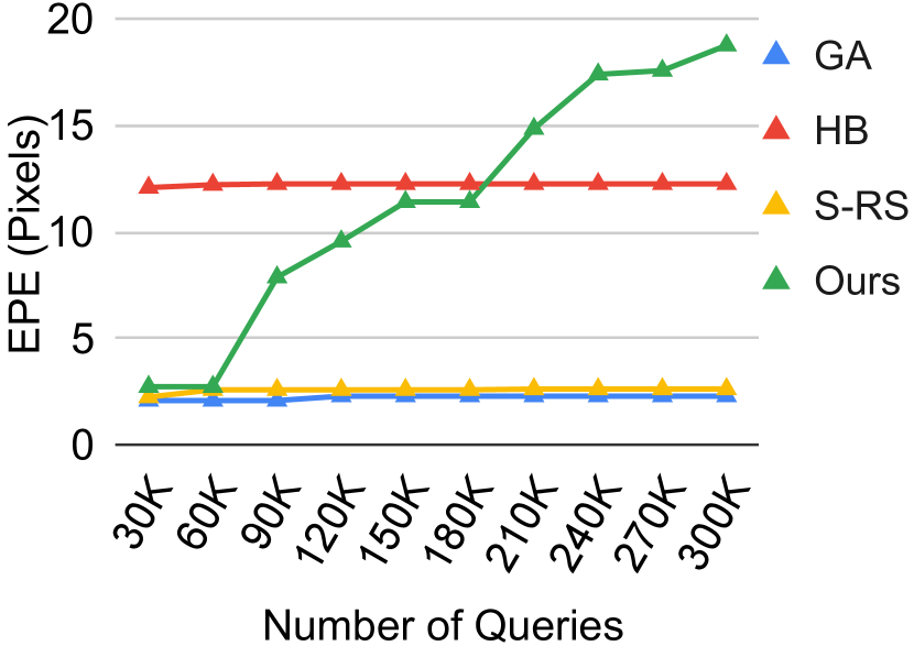
In this section, we compare the query efficiency of BadPart with baseline methods on the two pixel-wise regression tasks. We use DepthHints and Planedepth as the target MDE models and FlowNetC and FlowNet2 as the target OFE models. We use $2\%$ patch size and report each method’s attack performance under different query times. The maximum query times are set to 300K. Figure 4 shows the result. As shown, on Depthhints, Planedepth and FlowNetC, BadPart achieves the best attack performance at various query times from the beginning. On FlowNet2, although HardBeat has a good attack performance at first, the effect is not increased with more queries. BadPart surpasses HardBeat at around 120K queries and causes about 19.63 EPE. Figure 12 in Appendix shows more results with 1% patch size. In conclusion, our method is more efficient in general as it delivers superior attack performance using fewer queries to the target model. This efficiency is attributable to the more precise gradient estimation within the strategically selected square areas in BadPart.

5.4 Ablation Studies

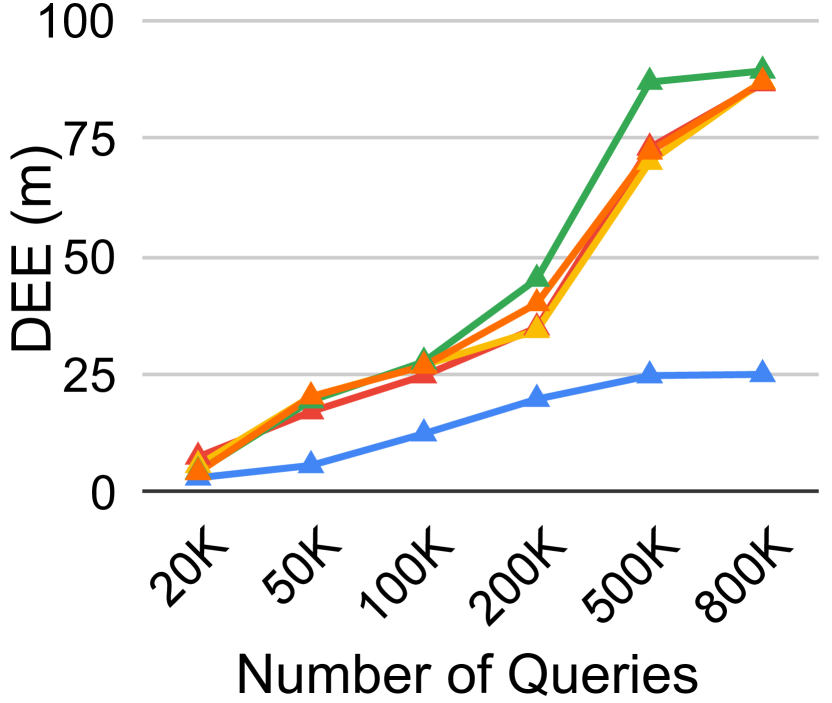
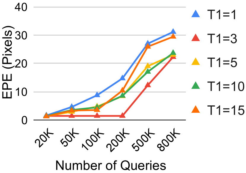
Number of Trials. In Alg. 3, we leverage $b$ random noises for gradient estimation. This number of trials balances the total query times and the accuracy of the estimated gradients. We evaluate BadPart utilizing different numbers of trials and report the attack performance on Monodepth2 and FlowNet2 under different query times. Results are presented in Figure 5. In the two subfigures, each line denotes a choice of the number of trials $b$ used in training, and the x-axis represents the number of queries and y-axis the corresponding attack performance. As shown, less trials (e.g., $b=1$) could decrease the accuracy of gradient estimation, hence impacting the attack performance, while large trials (e.g., $b=30$) would require more query times and degrade the efficiency. $b=20$ achieves a good balance in our study and is utilized as the default settings.

(a) Monodepth2

(b) FlowNet2

Figure 5: Ablation study on different number of trials $b$.

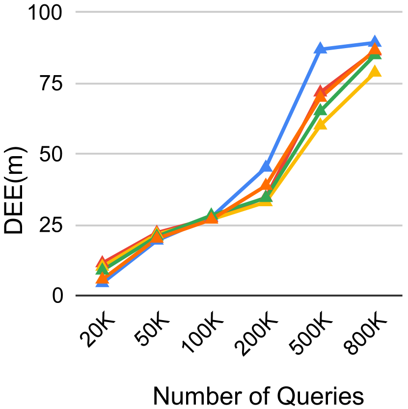
Intra-square Threshold. The intra-square threshold $T_{1}$ in Alg. 1 (line 21) controls the tolerance for negative update steps within the square area. Upon reaching this threshold, a different square location will be chosen. We have adjusted the threshold, ranging from 1 to 15, to evaluate the attack performance on Monodepth2 and FlowNet2 under various query times. Figure 6 presents the result. As shown, BadPart yields optimal performance on both models when $T_{1}$ is set to 1, and it is adopted as our default setting. Further ablation studies concerning the hyper-parameter $T_{2}$ and the locations of the patch can be found in Appendix B.

(a) Monodepth2

(b) FlowNet2

Figure 6: Ablation study on different intra-square threshold $T_{1}$.

Design Choices. We also conduct ablation studies to investigate the impact of our design choices. As shown in Figure 2, our method incorporates innovative designs of probabilistic sampling (PS), score normalization (SN) and adaptive scaling (AS). We assess various combinations of these designs and report the attack performance on Monodepth2 and FlowNet2 with 300K query times. Results are shown in Table 2. As shown, the integration of all three design choices yielded the best attack performance for both models. When considering each design individually, PS makes the most significant contribution and delivers the second-best performance. The other two designs can also enhance the performance to some extent. In summary, each of our unique designs plays a vital role in BadPart, with PS providing the most significant boost to performance.

Table 2: Ablation study on different design choices.

SN	AS	PS	Monodepth2	FlowNet2
			38.41	6.90
		$\checkmark$	54.88	15.19
	$\checkmark$		43.86	3.39
$\checkmark$			41.96	8.75
$\checkmark$	$\checkmark$		52.28	4.89
$\checkmark$	$\checkmark$	$\checkmark$	60.46	17.13

• * SN: Score Normalization, AS: Adaptive Scaling, PS: Probabilistic Sampling.

Figure 7: Attack Google MDE API (Google3DPortrait, ).

5.5 Attack Online Service

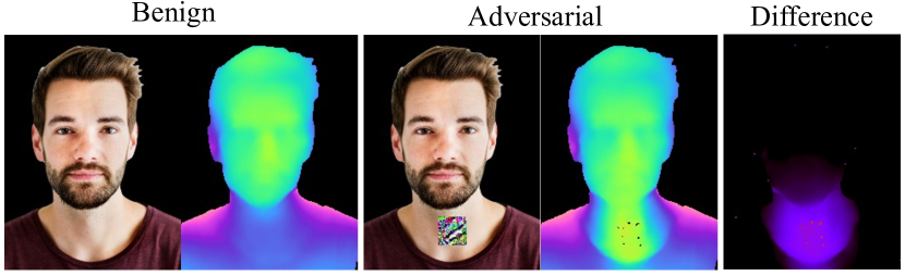
To evaluate the feasibility of BadPart in real-world applications, we conduct attacks on the Google API for portrait depth estimation (Google3DPortrait, ). Note that the model is not deployed by authors and we only query it for depth estimation. We utilize ten $256\times 192$ portrait images as training set and generate a $31\times 31$ patch using 50K queries to the API. Our attack goal is to minimize the estimated distance of the patched area on the portrait. BadPart has successfully reduced the mean depth estimation of the patched area by 43.5% from 0.431 cm to 0.243 cm. Figure 7 shows qualitative results. This adversarial example is available in the supplementary material, which can be uploaded to (Google3DPortrait, ) for efficacy validation. The adversarial patch can also be employed for beneficial purposes, such as privacy protection. By attaching the patch to personal images before publishing, individuals can prevent unauthorized use of their photos in such video composition services.

5.6 Defensive Discussion

As pioneers in the exploration of black-box adversarial patch attacks against pixel-wise regression tasks, we find ourselves in uncharted territory with no existing defense techniques specifically tailored for this context. Nevertheless, there are defense strategies designed against black-box attacks on classification models. For example, certifiable defenses such as PatchCleanser (Xiang et al., 2022) employ a mask to traverse all input positions, monitoring output class mutations to identify the most suspicious position. Furthermore, universal adversarial patch detection methods (e.g., SentiNet (Chou et al., 2020)) depend on the input features responsible for the predicted class to locate the patch. However, their reliance on class output renders them unsuitable for direct application to the pixel-wise regression tasks. In contrast, query-based defense techniques, designed to detect malicious queries by black-box attacks, may be more applicable to our context. Blacklight (Li et al., 2022), a leading defense of this type, leverages the similarity among different query inputs to detect black-box attacks. Its primary strategy involves calculating the hash representation of each incoming query and identifying an adversarial query if the hash matches any previous one. Blacklight’s efficacy is contingent on the similarity between two images in consecutive queries, which is a major feature of single-image black-box attacks (e.g., SquareAttack (Andriushchenko et al., 2020)). However, BadPart is a universal adversarial patch attack that does not depend on sample similarity, and the randomness in different samples could potentially enhance the universal effectiveness of the generated patch. Hence we add random noise on each attack sample to by-pass the defense. Additionally, the high resolution of our input images further diminishes the efficiency and efficacy of such a defense. To assess the defensive performance of Blacklight on BadPart, we have incorporated it in our framework and evaluated its detection rate for varying amounts of queries. The results are presented in Table 3. As shown, for both MDE and OFE tasks, the detection rate remains zero under 800K queries, while the attack performance is not affected and continues to increase with more queries. We discuss the limitations and our future work in Appendix D.

Table 3: Bypassing the query-based defense.

	Monodepth2		FlowNet2
Query	DEE	Detection Rate	EPE	Detection Rate
50K	20.28	0%	1.93	0%
200K	36.87	0%	8.24	0%
400K	73.27	0%	19.06	0%
800K	88.87	0%	25.53	0%

6 Conclusion

We propose BadPart, the first unified black-box adversarial patch attack against pixel-wise regression tasks, aiming at identifying vulnerabilities in visual regression models under query-based black-box attacks. BadPart utilizes square-based optimization, probabilistic square sampling and score-based gradient estimation, overcoming the scalability issues faced by previous black-box patch attacks. On 7 models across 2 typical pixel-wise regression tasks, our experiments compare BadPart with 3 baseline attack methods, validating the efficacy and efficiency of our method.

7 Broader Impact Statements

The unified adversarial patch attack we proposed against pixel-wise regression models aims to disclose the vulnerabilities in such models under query-based black-box attacks. Our work highlights potential security risks in applications that rely on those models, such as autonomous driving, virtual reality and video compositions. We hope to draw the attention of the related developers, and motivate the machine learning (ML) community to create more robust models or defense mechanisms against these types of attacks. This study around the robustness of models is aligned with many prior works/attacks in the ML community, and aims to advance the field of ML. Nevertheless, it is also worth mentioning that our technique can be used for benign purposes, like privacy protection, as we discussed in §5.5.

Appendix

Appendix A Experimental Details

Attack Settings. Adversarial patches are generated utilizing a single GPU (Nvidia RTX A6000) equipped with a memory capacity of 48G, in conjunction with an Intel Xeon Silver 4214R CPU. The resolution of input scenes from the KITTI dataset is resized to $384\times 1280$ for Planedepth and $320\times 1024$ for other models. We establish the initial square area as 2.5% of the patch area, and the pre-defined square size schedule (Algorithm 2 line 4) is set at $100,500,1500,3000,5000,10000$ for a maximum of 10000 iterations. The square area is halved once the iteration index reaches the pre-defined steps. The initial noise bound $\alpha$ (Algorithm 1 line 7) and noise decay factor $\gamma$ (Algorithm 1 line 23) are set to $0.1$ and $0.98$ respectively. The initialization period $K$ (Algorithm 2 line 5) is $100$ iterations. We adopt an Adam optimizer with the learning rate of $0.1$, and set $0.5$ for both $\beta_{1}$ and $\beta_{2}$. The reference white-box attack in Table 1 also employs the same Adam optimizer, while the gradients for the patch region are calculated through back-propagation. Other hyper-parameters are discussed in the ablation studies, in which we use $b=20$, $T_{1}=1$ and $T_{2}=1$ as the default settings.

Runtime Overhead. Table 4 displays the time used to generate a valid universal adversarial patch after $300K$ queries for both MDE and OFE models. The patch size is $2\%$ of the input image. The first column displays the target model name. The second column denotes the attack performance and the last column reports the runtime overhead of the patch generation.

Table 4: Attack performance and runtime overhead at 300K queries.

Models	DEE / EPE	Runtime
Monodepth2	74.71	0.5 h
Depthhints	38.54	0.5 h
Planedepth	21.03	4 h
SQLdepth	41.62	4 h
FlowNetC	695.55	0.5 h
FlowNet2	19.63	1 h
PWC-Net	3.81	2 h

Table 5: Attack performance on different patch locations.

Query	DepthHints	FlowNetC
50K	2.85	4.96
200K	20.99	128.39
400K	33.15	315.30
800K	42.63	447.57
1000K	46.56	483.54

Appendix B Additional Ablation Studies

Inter-square Threshold. The inter-square threshold $T_{2}$ in Algorithm 1 (line 23) controls the tolerance for negative iterations of square location selection. Upon reaching this threshold, BadPart reduces the noise bound $\epsilon$ for those trials in gradient estimation. Figure 8 presents the results of our experimental ablations on this parameter. As shown, its influence on the attack performance is not substantial, except for a large value setting on FlowNet2 (e.g., $T_{2}=15$). Consequently, we have set $T_{2}$ to 1 in our main experiments.

(a) Monodepth2

(b) FlowNet2

Figure 8: Ablation study on different inter-square threshold $T_{2}$.

Patch Locations. In consideration of different patch locations, BadPart can be easily extended to generate not only a scene-independent but also location-independent adversarial patch. For every step in optimizing the square area of adversarial patch in Algorithm 1(line 14-22), we randomly attach the adversarial patch on $K$ different positions ${\mathbf{q_{1}},...,\mathbf{q_{k}}}$. For each position $\mathbf{q_{i}}$, we get the estimated gradient $\mathbf{g_{i}}$ by Algorithm 3. The final gradient $\mathbf{g}$ is the average of ${\mathbf{g_{1}},...,\mathbf{g_{k}}}$. Then the current square area of adversarial patch is optimized by the estimated gradient $\mathbf{g}$. In our experiment, we utilize Depthhints and FlowNetC as our target models and the number of patch positions $K$ is set to 3. During the training stage, we randomly sample 5 patch locations on the validation images $[\mathbf{x^{v}}]_{n}$. In testing, we evaluate the attack performance on 100 random patch locations in the test set. Other settings remain the same as the previous experiments. Table 5 shows the result. We report the attack performance on two models, DepthHints and FlowNetC, under various query times. The average DEE/EPE caused by the adversarial patch on 100 random positions continues growing with queries rising after 1000K queries. Some qualitative examples are shown in Figure 9, using the converged patch. Columns represent various scenes. Each row in two Figures denotes a input-output pair of the target MDE/OFE model. The first two rows belong to Depthhints while the last two rows belong to FlowNetC. We can see that the adversarial patch generated by BadPart leads to significant error universally across both varying scenes and patch locations, which suggests that the patch exhibits robust characteristics of scene and location invariance.

Figure 9: Qualitative examples of the attack performance for different patch locations.

Figure 10: More qualitative examples of the attack performance of BadPart and the baseline methods on different models.

Table 6: More quantitative results of attack performance at 300K query times.

	57 * 57 Patch (1 %)				80 * 80 Patch (2 %)				100 * 100 Patch (3 %)
Models	GA	HB	S-RS	Ours	GA	HB	S-RS	Ours	GA	HB	S-RS	Ours
Monodepth2	-0.03	3.62	36.29	20.37	-0.17	19.64	57.72	66.21	0.61	18.03	77.33	81.98
DepthHints	0.30	2.20	1.63	39.11	-0.76	3.50	5.65	38.54	-1.47	2.24	40.24	42.40
SQLDepth	-0.14	-0.02	3.89	36.28	-0.43	0.12	15.31	41.39	-0.57	0.45	8.17	42.31
PlaneDepth	-0.43	0.83	0.83	17.19	-1.75	1.07	0.99	21.03	-1.86	1.47	2.47	19.39
FlowNetC	5.42	3.70	5.24	463.30	3.66	3.62	347.10	695.50	4.58	4.43	304.70	455.60
FlowNet2	2.28	12.21	2.64	18.75	1.67	7.22	1.77	19.63	1.27	10.31	2.96	11.05
PWC-Net	1.93	2.07	2.35	3.69	1.73	1.90	1.66	3.81	1.43	1.53	1.44	2.96

Appendix C More Qualitative and Quantitative Results

Figure 10 and Figure 11 show more qualitative results of our attack. Each row in the two Figures denotes a target model. The first four rows are MDE models and the last three rows are OFE models. The columns in Figure 10 denote different attack methods and the columns in Figure 11 represent various scenes. For MDE models, since the attack goal is to make the distance estimation as far as possible, darker colors in the estimated depth map for the patched area refer to better attack performance. For OFE models, since the adversarial patch is attached at the same position on the two input images, the ground-truth optical flow of the patched area should be zero (i.e., white color in the flow map). Hence, in the estimated flow map, stronger colors at the patched area represent better attack performance. The patches in Figure 10 are generated using 300K queries and they cover 2% of the image size. Quantitative results are presented in Table 6 as well as other patch sizes. It is easy to learn from Figure 10 and Table 6 that BadPart has the best attack performance on various pixel-wise regression models. In addition, Figure 11 shows that the generated patch works universally across varying scenes.

Figure 11: Qualitative examples of the attack performance of BadPart on different models and scene images.

(a) Depthhints

(b) Planedepth

(c) FlowNetC

(d) FlowNet2

Figure 12: Comparison of query efficiency between BadPart and the baseline methods on four models (1% patch).

Appendix D Limitations and Future Work

In this work, we have explored the black-box adversarial patch attack against pixel-wise regression models, which reveals the potential vulnerabilities in such models and their expanded applications. We have addressed the domain-specific challenge of high-resolution patch optimization, and our proposed method has shown an attack efficacy that surpasses that of various established benchmarks. It also appears to be robust against state-of-the-art black-box defense mechanisms. However, it is important to acknowledge potential limitations of our study. Our focus was predominantly on digital-space attacks, wherein the perturbed pixels are utilized directly as input for the model. This approach aligns with the conventional methods employed in prior black-box attacks, as referenced in works such as (Andriushchenko et al., 2020; Croce et al., 2022; Tao et al., 2023), and is deemed practical within the threat model that encompasses attacks on online services. Nevertheless, the implications of physical-world attacks are arguably more profound, particularly in the context of autonomous driving. Physical-world attacks, such as those described in (Cheng et al., 2022), necessitate a more nuanced consideration of environmental factors, including but not limited to viewing angles, distances, lighting conditions, and printing qualities. The question of how to effectively execute query-based black-box patch attacks in a physical setting remains unresolved. It is this intriguing challenge that we aim to address in our future research endeavors. An additional constraint pertains to the dimensions of the adversarial patch. Should individuals seek to employ such patches for the purpose of privacy preservation, as discussed in §5.5, the current manifestation of the patch on portrait images may be conspicuously apparent. The generation of stealthy patches for pixel-wise regression tasks within a black-box context is an unresolved issue, and we earmark this as a topic for future investigation.

References

- Alzantot et al. (2019) Alzantot, M., Sharma, Y., Chakraborty, S., Zhang, H., Hsieh, C.-J., and Srivastava, M. B. Genattack: Practical black-box attacks with gradient-free optimization. In Proceedings of the genetic and evolutionary computation conference, pp. 1111–1119, 2019.
- Andriushchenko et al. (2020) Andriushchenko, M., Croce, F., Flammarion, N., and Hein, M. Square attack: a query-efficient black-box adversarial attack via random search. In European conference on computer vision, pp. 484–501. Springer, 2020.
- Bae et al. (2021) Bae, G., Budvytis, I., and Cipolla, R. Estimating and exploiting the aleatoric uncertainty in surface normal estimation. In Proceedings of the IEEE/CVF International Conference on Computer Vision, pp. 13137–13146, 2021.
- Bang et al. (2017) Bang, J., Lee, D., Kim, Y., and Lee, H. Camera pose estimation using optical flow and orb descriptor in slam-based mobile ar game. In 2017 International Conference on Platform Technology and Service (PlatCon), pp. 1–4. IEEE, 2017.
- Chen et al. (2020) Chen, J., Jordan, M. I., and Wainwright, M. J. Hopskipjumpattack: A query-efficient decision-based attack. In 2020 ieee symposium on security and privacy (sp), pp. 1277–1294. IEEE, 2020.
- Chen et al. (2017) Chen, P.-Y., Zhang, H., Sharma, Y., Yi, J., and Hsieh, C.-J. Zoo: Zeroth order optimization based black-box attacks to deep neural networks without training substitute models. In Proceedings of the 10th ACM workshop on artificial intelligence and security, pp. 15–26, 2017.
- Chen et al. (2019) Chen, X., Liu, S., Xu, K., Li, X., Lin, X., Hong, M., and Cox, D. Zo-adamm: Zeroth-order adaptive momentum method for black-box optimization. Advances in neural information processing systems, 32, 2019.
- Cheng et al. (2022) Cheng, Z., Liang, J., Choi, H., Tao, G., Cao, Z., Liu, D., and Zhang, X. Physical attack on monocular depth estimation with optimal adversarial patches. In European Conference on Computer Vision, pp. 514–532. Springer, 2022.
- Cheng et al. (2023) Cheng, Z., Choi, H., Liang, J., Feng, S., Tao, G., Liu, D., Zuzak, M., and Zhang, X. Fusion is not enough: Single-modal attacks to compromise fusion models in autonomous driving. arXiv preprint arXiv:2304.14614, 2023.
- Chou et al. (2020) Chou, E., Tramer, F., and Pellegrino, G. Sentinet: Detecting localized universal attacks against deep learning systems. In 2020 IEEE Security and Privacy Workshops (SPW), pp. 48–54. IEEE, 2020.
- (11) Clipdrop. Portrait Depth Estimation. https://clipdrop.co/apis/docs/portrait-depth-estimation.
- Croce et al. (2022) Croce, F., Andriushchenko, M., Singh, N. D., Flammarion, N., and Hein, M. Sparse-rs: a versatile framework for query-efficient sparse black-box adversarial attacks. In Proceedings of the AAAI Conference on Artificial Intelligence, volume 36, pp. 6437–6445, 2022.
- Dosovitskiy et al. (2015) Dosovitskiy, A., Fischer, P., Ilg, E., Hausser, P., Hazirbas, C., Golkov, V., Van Der Smagt, P., Cremers, D., and Brox, T. Flownet: Learning optical flow with convolutional networks. In Proceedings of the IEEE international conference on computer vision, pp. 2758–2766, 2015.
- Duan et al. (2021) Duan, R., Mao, X., Qin, A. K., Chen, Y., Ye, S., He, Y., and Yang, Y. Adversarial laser beam: Effective physical-world attack to dnns in a blink. In Proceedings of the IEEE/CVF Conference on Computer Vision and Pattern Recognition, pp. 16062–16071, 2021.
- Feng et al. (2022) Feng, Y., Wu, B., Fan, Y., Liu, L., Li, Z., and Xia, S.-T. Boosting black-box attack with partially transferred conditional adversarial distribution. In Proceedings of the IEEE/CVF Conference on Computer Vision and Pattern Recognition, pp. 15095–15104, 2022.
- Gao et al. (2020) Gao, L., Zhang, Q., Song, J., Liu, X., and Shen, H. T. Patch-wise attack for fooling deep neural network. In Computer Vision–ECCV 2020: 16th European Conference, Glasgow, UK, August 23–28, 2020, Proceedings, Part XXVIII 16, pp. 307–322. Springer, 2020.
- Godard et al. (2019) Godard, C., Mac Aodha, O., Firman, M., and Brostow, G. J. Digging into self-supervised monocular depth estimation. In Proceedings of the IEEE/CVF international conference on computer vision, pp. 3828–3838, 2019.
- (18) Google3DPortrait. 3D Portrait. https://storage.googleapis.com/tfjs-models/demos/3dphoto/index.html.
- He et al. (2021) He, Y., Meng, G., Chen, K., Hu, X., and He, J. DRMI: A dataset reduction technology based on mutual information for black-box attacks. In 30th USENIX Security Symposium (USENIX Security 21), pp. 1901–1918, 2021.
- Ilg et al. (2017) Ilg, E., Mayer, N., Saikia, T., Keuper, M., Dosovitskiy, A., and Brox, T. Flownet 2.0: Evolution of optical flow estimation with deep networks. In Proceedings of the IEEE conference on computer vision and pattern recognition, pp. 2462–2470, 2017.
- Ilie et al. (2021) Ilie, A., Popescu, M., and Stefanescu, A. Evoba: An evolution strategy as a strong baseline for black-box adversarial attacks. In International Conference on Neural Information Processing, pp. 188–200. Springer, 2021.
- Ilyas et al. (2018) Ilyas, A., Engstrom, L., Athalye, A., and Lin, J. Black-box adversarial attacks with limited queries and information. In International conference on machine learning, pp. 2137–2146. PMLR, 2018.
- Karpathy (2020) Karpathy, A. Tesla use per-pixel depth estimation with self-supervised learning, 2020. https://youtu.be/hx7BXih7zx8?t=1334.
- Lambert (2021) Lambert, F. Hacker shows what Tesla Full Self-Driving’s vision depth perception neural net can see, 2021. https://electrek.co/2021/07/07/hacker-tesla-full-self-drivings-vision-depth-perception-neural-net-can-see/.
- Lenssen et al. (2020) Lenssen, J. E., Osendorfer, C., and Masci, J. Deep iterative surface normal estimation. In Proceedings of the ieee/cvf conference on computer vision and pattern recognition, pp. 11247–11256, 2020.
- Li et al. (2020) Li, H., Xu, X., Zhang, X., Yang, S., and Li, B. Qeba: Query-efficient boundary-based blackbox attack. In Proceedings of the IEEE/CVF conference on computer vision and pattern recognition, pp. 1221–1230, 2020.
- Li et al. (2022) Li, H., Shan, S., Wenger, E., Zhang, J., Zheng, H., and Zhao, B. Y. Blacklight: Scalable defense for neural networks against Query-BasedBlack-Box attacks. In 31st USENIX Security Symposium (USENIX Security 22), pp. 2117–2134, 2022.
- Liew et al. (2023) Liew, J. H., Yan, H., Zhang, J., Xu, Z., and Feng, J. Magicedit: High-fidelity and temporally coherent video editing. In arXiv, 2023.
- Liu et al. (2016) Liu, Y., Chen, X., Liu, C., and Song, D. Delving into transferable adversarial examples and black-box attacks. arXiv preprint arXiv:1611.02770, 2016.
- Menze et al. (2015) Menze, M., Heipke, C., and Geiger, A. Joint 3d estimation of vehicles and scene flow. In ISPRS Workshop on Image Sequence Analysis (ISA), 2015.
- Moon et al. (2019) Moon, S., An, G., and Song, H. O. Parsimonious black-box adversarial attacks via efficient combinatorial optimization. In International conference on machine learning, pp. 4636–4645. PMLR, 2019.
- Ranjan et al. (2019) Ranjan, A., Janai, J., Geiger, A., and Black, M. J. Attacking optical flow. In Proceedings of the IEEE/CVF International Conference on Computer Vision, pp. 2404–2413, 2019.
- Sun et al. (2018) Sun, D., Yang, X., Liu, M.-Y., and Kautz, J. Pwc-net: Cnns for optical flow using pyramid, warping, and cost volume. In Proceedings of the IEEE conference on computer vision and pattern recognition, pp. 8934–8943, 2018.
- Tao et al. (2023) Tao, G., An, S., Cheng, S., Shen, G., and Zhang, X. Hard-label black-box universal adversarial patch attack. In 32nd USENIX Security Symposium (USENIX Security 23), pp. 697–714, 2023.
- Teed & Deng (2020) Teed, Z. and Deng, J. Raft: Recurrent all-pairs field transforms for optical flow. In Computer Vision–ECCV 2020: 16th European Conference, Glasgow, UK, August 23–28, 2020, Proceedings, Part II 16, pp. 402–419. Springer, 2020.
- (36) Tesla. Tesla Autopilot. https://www.tesla.com/autopilot.
- Uhrig et al. (2017) Uhrig, J., Schneider, N., Schneider, L., Franke, U., Brox, T., and Geiger, A. Sparsity invariant cnns. In International Conference on 3D Vision (3DV), 2017.
- Wang et al. (2023a) Wang, R., Yu, Z., and Gao, S. Planedepth: Self-supervised depth estimation via orthogonal planes. In Proceedings of the IEEE/CVF Conference on Computer Vision and Pattern Recognition, pp. 21425–21434, 2023a.
- Wang & He (2021) Wang, X. and He, K. Enhancing the transferability of adversarial attacks through variance tuning. In Proceedings of the IEEE/CVF Conference on Computer Vision and Pattern Recognition, pp. 1924–1933, 2021.
- Wang et al. (2023b) Wang, Y., Liang, Y., Xu, H., Jiao, S., and Yu, H. Sqldepth: Generalizable self-supervised fine-structured monocular depth estimation. arXiv preprint arXiv:2309.00526, 2023b.
- Wang et al. (2021) Wang, Z., Guo, H., Zhang, Z., Liu, W., Qin, Z., and Ren, K. Feature importance-aware transferable adversarial attacks. In Proceedings of the IEEE/CVF international conference on computer vision, pp. 7639–7648, 2021.
- Watson et al. (2019) Watson, J., Firman, M., Brostow, G. J., and Turmukhambetov, D. Self-supervised monocular depth hints. In Proceedings of the IEEE/CVF International Conference on Computer Vision, pp. 2162–2171, 2019.
- Wimbauer et al. (2021) Wimbauer, F., Yang, N., Von Stumberg, L., Zeller, N., and Cremers, D. Monorec: Semi-supervised dense reconstruction in dynamic environments from a single moving camera. In Proceedings of the IEEE/CVF Conference on Computer Vision and Pattern Recognition, pp. 6112–6122, 2021.
- Wu et al. (2020) Wu, D., Wang, Y., Xia, S.-T., Bailey, J., and Ma, X. Skip connections matter: On the transferability of adversarial examples generated with resnets. arXiv preprint arXiv:2002.05990, 2020.
- Xiang et al. (2022) Xiang, C., Mahloujifar, S., and Mittal, P. PatchCleanser: Certifiably robust defense against adversarial patches for any image classifier. In 31st USENIX Security Symposium (USENIX Security 22), pp. 2065–2082, 2022.
- Yan et al. (2020) Yan, Z., Guo, Y., Liang, J., and Zhang, C. Policy-driven attack: learning to query for hard-label black-box adversarial examples. In International Conference on Learning Representations, 2020.
- Yu et al. (2018) Yu, C., Wang, J., Peng, C., Gao, C., Yu, G., and Sang, N. Bisenet: Bilateral segmentation network for real-time semantic segmentation. In Proceedings of the European conference on computer vision (ECCV), pp. 325–341, 2018.
- Zeng et al. (2019) Zeng, J., Tong, Y., Huang, Y., Yan, Q., Sun, W., Chen, J., and Wang, Y. Deep surface normal estimation with hierarchical rgb-d fusion. In Proceedings of the IEEE/CVF conference on computer vision and pattern recognition, pp. 6153–6162, 2019.
- Zhang et al. (2021) Zhang, J., Li, L., Li, H., Zhang, X., Yang, S., and Li, B. Progressive-scale boundary blackbox attack via projective gradient estimation. In International Conference on Machine Learning, pp. 12479–12490. PMLR, 2021.
- Zhou et al. (2022) Zhou, T., Wang, W., Konukoglu, E., and Van Gool, L. Rethinking semantic segmentation: A prototype view. In Proceedings of the IEEE/CVF Conference on Computer Vision and Pattern Recognition, pp. 2582–2593, 2022.