Estimating sample paths of Gauss-Markovprocesses from noisy data
Benjamin Davies
Department of Economics, Stanford University; bldavies@stanford.edu.
(Draft version: )
Abstract
I derive the pointwise conditional means and variances of an arbitrary Gauss-Markov process, given noisy observations of points on a sample path.
These moments depend on the process’s mean and covariance functions, and on the conditional moments of the sampled points.
I study the Brownian motion and bridge as special cases.
Keywords: Gaussian process, Markov process, Brownian motion, noisy data
1 Introduction
Suppose we observe data generated by the process
(1)
where is non-decreasing in , where is unknown, and where the errors are jointly normally distributed (hereafter “Gaussian”) with independently of .
We use to construct pointwise estimates
with mean squared error (MSE)
(2)
In this note, I derive expressions for and when is a sample path of a Gauss-Markov process.
Such processes have two defining properties:
(G)
For every finite subset , the vector is multivariate Gaussian;
(M)
If , then and are conditionally independent given .
Property (G) implies that is Gaussian, and so its distribution is fully determined by its mean and variance .
Theorem 1 expresses these moments in terms of the means and (co)variances of the .
This allows me to construct the estimate and its MSE at all points .
This estimate optimally extrapolates from, or interpolates between, the observations in .111
The estimate is “optimal” in that it minimizes the MSE (2) for all .
I let these observations be noisy, with Gaussian errors .
This allows me to extend analyses that assume observations have no noise (e.g., Bardhi, , 2024; Callander, , 2011; Carnehl and Schneider, , 2023).222Rasmussen and Williams, (2006, p. 16) derive expressions for and when follows a Gaussian (but not necessarily Markov) process and the errors are iid.
I impose the Markov property (M) to obtain (relatively) closed-form expressions for and .
I also allow for arbitrary (co)variances in the .
I also let the sampled points be less or greater than the target point .
This contrasts with Davies, (2024), who studies sequential learning from noisy observations of a sample path.
Such learning always involves extrapolation, whereas I allow for interpolation.
2 Preliminaries
The data contain noisy observations of the values .
These observations equal the sum of two Gaussian random variables and so are Gaussian too.
Moreover, by property (G), the vector is multivariate Gaussian for all .
It follows that
is also multivariate Gaussian.
Consequently, we can construct the conditional distribution of given using a well-known result about multivariate Gaussian variables:
Lemma 1.
Let and be integers, and let be multivariate Gaussian with mean and variance .
Partition into vectors and , and let and
be the corresponding partitions of and .
If is invertible, then
(3)
See Bishop, (2006, p. 87) or DeGroot, (2004, p. 55) for proofs of this lemma, and Appendix A for proofs of my other results.
Substituting and into (3) provides expressions for the moments of .
I refine these expressions by imposing properties (G) and (M).
Property (G) comes from being a sample path of a Gaussian process.333
Gaussian processes are stochastic processes satisfying by property (G).
For more information on these processes and their applications, see Section 6.4 of Bishop, (2006) or Chapter 2 of Rasmussen and Williams, (2006).
This process can be characterized by
1.
A mean function with for all , and
2.
A covariance function with for all .
For convenience, I define a variance function by for all .
The values of , , and are known for all , but the values of are not.
Property (M) comes from being a sample path of a Markov process.
It allows me to focus on the conditional distribution of given at most two values : those with closest to .
Lemma 2 characterizes this conditional distribution.
Lemma 2.
Let be a sample path of a Gauss-Markov process, let be arbitrary, and define
(4)
Then is Gaussian with mean
(5)
and variance
(6)
and is Gaussian with mean
and variance
For example, suppose for some .
Lemma 2 characterizes the distributions of and when the values of and are known.
However, variation in the errors makes the values of and unknown.
So the conditional means of and given are random.
But their conditional variances given are not random; by Lemma 2, these variances depend on only the known values of the variance function and covariance function .
3 Conditional moments of a Gauss-Markov process
Theorem 1 refines Lemma 1 by imposing properties (G) and (M).
Specifically, it characterizes the mean and variance of when is a sample path of an arbitrary Gauss-Markov process.
These moments depend on the location of relative to the points at which contains noisy observations of .
Theorem 1.
Let be a sample path of a Gauss-Markov process.
Suppose is generated by the process (1), where is non-decreasing in and the errors are jointly Gaussian with independently of .
Then is Gaussian for all .
Moreover:
If , then the estimate of is linear in the estimate of .
Conversely, if , then is linear in the estimate of .
In both cases, we can construct in two steps:
1.
Use to estimate the “boundary” values and ;
2.
Extrapolate from the closest boundary estimate.
For example, suppose contains one observation with error .
Then
is linear in the deviation of from its mean .
Intuitively, this deviation provides information about the difference , which the factor translates into information about the difference .
This factor is larger when the covariance of and is larger, and when the variance of is smaller.
If and , then we can construct in three steps:
1.
Find an index for which ;
2.
Use to estimate the values of and ;
3.
Interpolate from the estimates and .
The interpolant is a weighted sum of the mean , the deviation , and the deviation .
The weights on the two deviations depend on the (co)variances of , , and , as well as the (co)variances of and .
Theorem 1 expresses the moments of in terms of the moments of the .
The latter moments can be computed analytically if is small (e.g., as in the case with above), or numerically if is large.
The expressions in Theorem 1 reveal how changing the moments of the changes the moments of .
4 Conditional moments of a Brownian motion
I now consider a specific Gauss-Markov process: a Brownian motion with known drift and scale , and unknown initial value .444
So the sample path solves the stochastic differential equation
where is an unknown sample path of a (standard) Wiener process.
This process has initial value and iid Gaussian increments .
This process has mean and covariance functions defined by
and
for all .555
Thus for all .
Substituting these expressions into Theorem 1 yields the following result.
Corollary 1.
Let be a sample path of a Brownian motion with drift , scale , and initial value .
Define as in Theorem 1.
Then is Gaussian for all .
Moreover:
(i)
If , then
and
(ii)
If for some , then
and
(iii)
If , then
and
If is a sample path of a Brownian motion, then the estimate of is piecewise linear in .
For example, consider the canonical case in which the initial value is known.
As increases from zero, the estimate
interpolates linearly between and , then between and , then between and , and so on until .
Beyond this point, the data provide no information about .
Consequently, the estimate treats as a Brownian motion with drift , scale , and (possibly random) initial value .
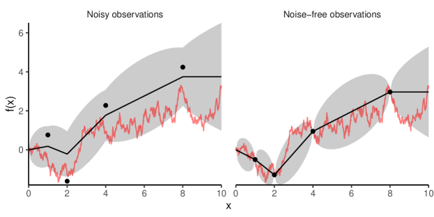
Figure 1: Learning about a Brownian motion from noisy and noise-free observationsNotes:
Red lines show sample path of Brownian motion with drift , scale , and initial value .
Black dots represent observations with and .
Black lines represent estimates of when .
Gray regions represent 90% confidence intervals, constructed analytically from the conditional variances defined in Corollary 1.
Left panel has iid; right panel has for each .
It shows how varies with when and the data contain observations with iid errors.
Figure 1 also shows the 90% confidence interval around , constructed analytically from the conditional variances defined in Corollary 1.
This interval expands as moves away from the sampled points .666
If is known (i.e., ) and the observations have no noise (i.e., for each ), then the MSE
attains its piecewise maxima at the midpoint of each piece.
Suppose the data are not noisy (i.e., for each ) and for some .
Then the distribution of coincides with the distribution obtained by assuming is a sample path of a Brownian bridge with scale , known initial value , and known terminal value .777
See, e.g., Section 5.6.B of Karatzas and Shreve, (1988) for more information about Brownian bridges.
Corollary 1(ii) generalizes to Brownian bridges with unknown initial and terminal values.
For example, suppose and that
for some means , variances , and correlation .
Then has mean
and variance
Choosing and yields the mean and variance for the Brownian bridge on with and .
References
Bardhi, (2024)
Bardhi, A. (2024).
Attributes: Selective Learning and Influence.
Econometrica, 92(2):311–353.
Bishop, (2006)
Bishop, C. M. (2006).
Pattern recognition and machine learning.
Springer, New York.
Callander, (2011)
Callander, S. (2011).
Searching and Learning by Trial and Error.
American Economic Review, 101(6):2277–2308.
Carnehl and Schneider, (2023)
Carnehl, C. and Schneider, J. (2023).
A Quest for Knowledge.
Davies, (2024)
Davies, B. (2024).
Learning about a changing state.
DeGroot, (2004)
DeGroot, M. H. (2004).
Optimal Statistical Decisions.
Wiley, first edition.
Karatzas and Shreve, (1988)
Karatzas, I. and Shreve, S. E. (1988).
Brownian Motion and Stochastic Calculus, volume 113 of Graduate Texts in Mathematics.
Springer New York, New York, NY.
Rasmussen and Williams, (2006)
Rasmussen, C. E. and Williams, C. K. I. (2006).
Gaussian processes for machine learning.
MIT Press, Cambridge, MA.
Now , , and are jointly Gaussian by property (G).
Therefore, by Lemma 1, both and are (univariate) Gaussian.
Choosing and in the statement of Lemma 1 yields (5) and (6), while choosing yields
The are sums of (jointly) Gaussian random variables, so they are also jointly Gaussian.
Thus is multivariate Gaussian.
It follows from Lemma 1 that is (univariate) Gaussian.
By property (M) and the errors’ independence of , we know is conditionally independent of given the values with closest to .
I use this fact to prove cases (i)–(iii):
(i)
Suppose .
Then is conditionally independent of given .
Thus
where holds by the law of total expectation and holds by Lemma 2.
Likewise
where holds by the law of total variance and holds by Lemma 2.
(ii)
Now suppose for some .
Then is conditionally independent of given and .
Thus
where holds by the law of total expectation and holds by Lemma 2.
Likewise
where holds by the law of total variance and holds by Lemma 2.
(iii)
Finally, suppose .
Then is conditionally independent of given .
The result follows from similar arguments used to prove case (i).∎