Metric Dimensions of Generalized Sierpiński Graphs over Squares
Abstract
Metric dimension is a valuable parameter that helps address problems related to network design, localization, and information retrieval by identifying the minimum number of landmarks required to uniquely determine distances between vertices in a graph. Generalized Sierpiński graphs represent a captivating class of fractal-inspired networks that have gained prominence in various scientific disciplines and practical applications. Their fractal nature has also found relevance in antenna design, image compression, and the study of porous materials. The hypercube is a prevalent interconnection network architecture known for its symmetry, vertex transitivity, regularity, recursive structure, high connectedness, and simple routing. Various variations of hypercubes have emerged in literature to meet the demands of practical applications. Sometimes, they are the spanning subgraphs of it. This study examines the generalized Sierpiński graphs over , which are spanning subgraphs of hypercubes and determines the metric dimension and their variants. This is in contrast to hypercubes, where these properties are inherently complicated. Along the way, the role of twin vertices in the theory of metric dimensions is further elaborated.
a Department of Mathematics, Rajalakshmi Engineering College, Thandalam, Chennai 602105, India
b Faculty of Mathematics and Physics, University of Ljubljana, Slovenia
c Institute of Mathematics, Physics and Mechanics, Ljubljana, Slovenia
d Faculty of Natural Sciences and Mathematics, University of Maribor, Slovenia
Keywords: metric dimension; edge metric dimension; fault-tolerant dimension; twin; fractal network; generalized Sierpiński graph
Mathematics Subject Classification (2020): 05C12, 68M15
1 Introduction
Parallel computing is a type of computation in which many calculations or processes are carried out simultaneously. This is in contrast to serial computing, where calculations are performed sequentially, one after the other. Parallel computing offers several advantages, including improved performance, scalability, and the ability to tackle larger and more complex problems [11]. However, designing and implementing parallel algorithms can be challenging due to issues such as synchronization, load balancing, and communication overhead [14]. Graph theory can have a significant impact on parallel computing, particularly in the context of algorithm design and optimization [9]. Graph theory provides a powerful framework for modeling and analyzing the structure and relationships of data, which is essential in many parallel computing applications. Many parallel computing applications involve graph algorithms, which operate on graphs to solve various problems such as shortest path finding, clustering, graph traversal, and network flow optimization [10]. Parallelizing these algorithms efficiently requires an understanding of both the graph structure and the characteristics of parallel computation.
A parallel computing network can indeed be viewed and represented as a graph structure. This representation can provide insights into the topology of the network, the communication patterns between computing nodes, and the distribution of computational tasks [39]. Each computing unit in the parallel computing network, whether it’s a processor core, a compute node, or a server, can be represented as a node in the graph. These nodes represent the individual processing elements that perform computations. The communication links between computing nodes are represented as edges in the graph. These edges depict the connectivity between nodes and can represent various types of communication channels, such as direct interconnects, network links, or shared memory connections. The arrangement of nodes and edges in the graph represents the network’s topology. This includes characteristics such as whether the network is a clustered architecture, a mesh, a torus, a hypercube, or another topology [13]. The choice of topology can impact factors like communication latency, bandwidth [42], and fault tolerance. Graph-based representations can also be used for performance analysis and optimization of parallel computing networks. Techniques such as graph partitioning, load balancing, and routing algorithms [6] can be applied to improve the efficiency and scalability of parallel computations. By representing a parallel computing network as a graph structure, we can gain insights into its characteristics, connectivity, and performance, which can aid in the design, analysis, and optimization of parallel algorithms and systems.
Graphic structures with self-similarity and recurrence are called fractals. Networks with fractal nature seems to be beneficial in the study of larger networks found in artificial and natural systems, such as neuroscience [17], music [38], social networking sites, and computers, allowing the subject of network science to progress. Images of complicated structures, such as neuronal dendrites or bacterial growth patterns [44] in culture, can be captured and analysed with the help of such networks. Sierpiński networks are one of that class and can be used in parallel computing systems, particularly in the design of parallel supercomputers and high-performance computing (HPC) clusters. The Sierpiński network is characterized by its recursive and self-similar structure. It consists of interconnected nodes arranged in a hierarchical manner, with each level of the hierarchy representing a smaller version of the overall network. The Sierpiński network is inherently scalable, allowing it to accommodate a large number of nodes or processors. The self-similar structure of the Sierpiński network enables efficient routing and communication patterns. Due to these characteristics, the Sierpiński network can be explored as a potential topology for parallel computing systems, particularly in research contexts where innovative network designs are investigated to improve scalability, performance, and fault tolerance in parallel computing environments. In a particular case when the base graph is , the Sierpiński networks are the Tower of Hanoi graphs with 3 pegs. Adding an open link to the extreme vertices of Sierpiński graphs results in WK-recursive networks. As abstract graphs, these networks were introduced in 1988 as message passing architectures and are employed in VLSI implementation [55]. A decade later, WK-recursive networks were equipped with the Sierpiński labelings and named Sierpiński graphs [31]. From then on the notion of Sierpiński graphs coincides with these graphs equipped with the Sierpiński labeling. The latter has also made it possible to explore Sierpiński graphs in more depth. Let us list some of the related results. This family of networks is proved to be Hamiltonian and the length of geodesic between their vertices are given in [31]. Some metric properties including the average eccentricity [24], connectivity [34] and median [3] are discussed. Some topological descriptors of Siepiński graphs are availabe in [25]. All shortest paths in Sierpiński graphs are discussed in [22]. The review paper [23] from 2017 summarizes the results on Sierpiński graphs and related classes of graphs and also proposes a classification of Sierpiński-like graphs.
The classical Sierpiński graphs as introduced in [31] use complete graphs are their basic stones. Replacing complete graphs by arbitrary graphs, generalized Sierpiński graphs were introduced in [18]. The key idea is again to create a recursive process that generates a fractal-like pattern within the graph. Generalized Sierpiński graphs are thus a broader class of fractal graphs that extend the concept of Sierpiński graphs to various shapes and structures beyond just complete graphs.
Let be a graph and a positive integer. Then the generalized Sierpiński graph is formally defined as follows. Set . Then , that is, vertices of are vectors of length , each coordinate being a vertex of . Two vertices and of are by definition adjacent if the following conditions hold for some index :
-
(i)
for ,
-
(ii)
and ,
-
(iii)
, for .
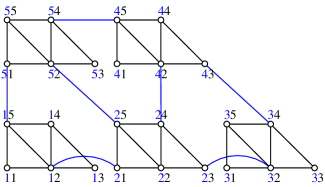
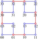
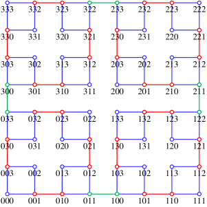
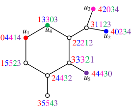
In Fig. 1, a graph with and are illustrated.

Generalized Sierpiński graphs are used to model polymer networks [16]. Chromatic, vertex cover, clique and domination numbers [52], roman domination [50], strong metric dimension [15] related results have been discussed for generalized Sierpiński graphs. In this article, we focus on the family and determine their metric dimension, edge metric dimension, fault-tolerant metric dimension and fault-tolerant edge metric dimension. The determination of these formulae is made possible by first examining in more detail the role of twin vertices in these dimensions.
2 The Problem and its Relevance
Sensors can be used to detect faults or anomalies in the nodes or communication links of a parallel computing network. By continuously monitoring system parameters, sensors can help identify hardware failures, software errors, or performance bottlenecks, enabling proactive maintenance and troubleshooting. They can be deployed to detect unauthorized access, malicious activities, or security breaches in a parallel computing network. By monitoring network traffic, system logs, and environmental conditions, sensors can help identify and mitigate security threats in real-time. By collecting and analyzing sensor data, administrators and operators can make informed decisions to optimize system operation and ensure the efficient and reliable execution of parallel computing workloads. While sensor deployment can offer significant benefits in terms of system performance, reliability, and efficiency, it’s essential to consider the associated costs, complexities, and trade-offs involved. Knowledge about metric dimension helps in optimizing sensor deployment.
2.1 Basis and Fault-tolerant Basis
Graph theory considers networks as topological graphs with interesting characteristics. Metric dimension is a measure of how efficiently one can locate and distinguish between the vertices (nodes) of a graph using a minimal set of landmarks or reference points [53, 19]. Metric dimension has applications in various fields, including network design [5], robotics [29], and location-based services. It helps in understanding how to place sensors or landmarks in a network to ensure efficient location determination [8, 7, 26, 43, 37]. Calculating the exact metric dimension of a graph is often a computationally challenging problem. For certain classes of graphs, such as trees, there are efficient algorithms to find the metric dimension. However, for general graphs [29], bipartite graphs [41] and directed graphs [49] determining the metric dimension is NP-hard. Despite the computational difficulty, the precise value of metric dimension is evaluated for many graph structures including honeycomb [40], butterfly [41], Beneš [41], Sierpiński [33], and irregular triangular networks [47]. The works related to metric dimension have been surveyed recently in [54].
The distance between two vertices in a connected graph , with vertex set and edge set , is equal to the number of edges in a geodesic (shortest path) connecting them. For a vertex and an edge the distance between them is given by, . For an ordered subset of vertices, every vertex of can be represented by a vector of distances
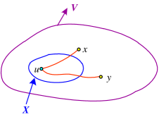
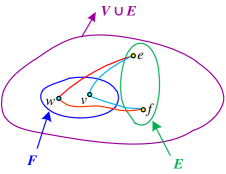
The subset is a metric generator (MG) if , . In other words, is a MG if every pair has at least one vertex such that , see Fig. 2.
A MG with minimum vertices is a (metric) basis; its cardinality is indicated by , which is the metric dimension. This concept is well-established in the literature, and has given rise to many different variations [1, 12, 27, 30]. One of these novel and highly motiated variations is known as fault-tolerant metric dimension. In this variation, the crucial aspect is that the selected set of vertices must still resolve the graph even when any one vertex from that set has become faulty or useless. That is, a set of vertices is termed as a fault-tolerant metric generator (FTMG) if, for every vertex within , the set obtained by removing from remains a MG for the graph. In other words, even in the absence of any single vertex in the set , the remaining vertices should still have the ability to resolve the graph.
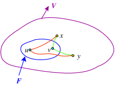
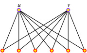
The term fault-tolerant metric dimension is denoted as , and it represents the minimum number of vertices required to form a FTMG for the graph . The set of vertices that achieves this minimum and serves as a FTMG is referred to as a fault-tolerant metric basis. FTMG can also be described as a set of vertices , with the property that for every pair of vertices and in the graph , there exist at least two vertices and in set , where and are at different distances from both and , see Fig. 3. A FTMG ensures that even if one vertex from the set is missing, there will still be another vertex in that can resolve and in the graph. This idea was first presented in [21] and was further discussed in [51, 4, 48, 2].
2.2 Edge Basis and Fault-tolerant Edge Basis
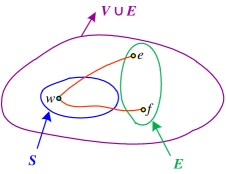
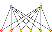
In a parallel computing system, data is transmitted between processors through an interconnection network, which is a complex arrangement of processors and communication links. Identifying and addressing the links (connections) within this network is crucial for quickly pinpointing any faulty connections. This task can be performed optimally by utilizing the smallest possible set of vertices that uniquely label every edge in the network. In this context, a set of vertices within a graph is referred to as an edge metric generator (EMG) if it satisfies the condition that for any two edges and in the graph , there exists a vertex in set such that and are distinct, see Fig. 4.
An EMG ensures that each edge in the network is uniquely identifiable based on its distance to the vertices in set . The number of vertices in the smallest possible EMG is referred to as the edge metric dimension and is connoted as . This variation was initially studied by Kelenc et al. [27], and they established its NP-completeness. Following the inception of this concept, numerous articles have emerged in this research field. To list a few, we have the characterization of graphs with maximum dimension [61, 59], the dimension of web graph, prism related graph, convex polytope graph [58], generalized Petersen graph [56], some classes of planar graph [57], Erdős-Renyi random graph [60], graph operations such as join, lexicographic, corona [45], and hierarchical products [32] for some graph classes. Identifying graphs with has gained more interest [36, 35].
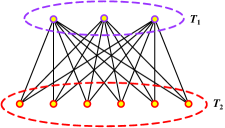
In order for an edge metric generator, denoted as , to be considered fault-tolerant, it must possess an additional property, which is that the set obtained by removing any vertex from must still be capable of resolving the edges in the graph . The minimum number of vertices required to form a fault-tolerant edge metric generator (FTEMG) is known as the fault-tolerant edge metric dimension, denoted as . As depicted in Fig. 5, in a FTEMG set , for any pair of edges and in the graph , there are at least two vertices and within the set that are at different distances from both and .
3 Effect of Twin Vertices on Metric Dimensions
In this section, we will clarify how twins vertices affect all the variations of the metric dimension we are interested in. Some of the results on this are known from before, but others are being added newly.
Let be a graph and . Then is the open neighbourhood of and is the closed neighbourhood of . A vertex is a twin vertex if there exists a vertex such that or . In the first case we say that and are non-adjacent twins (also known as false twins), in the second case they are adjacent twins (also known as true twins). A maximal set of vertices in which every two vertices are twins, is called a twin set. These concepts are illustrated in Fig. 6.
In [20, Corollary 2.4] it was observed that if is a resolving set of a connected graph and and are twins, then , cf. [46, 48]. From this fact, the following conclusions can be easily drawn.
Proposition 3.1.
In the case of bipartite graphs, (fault-tolerant) metric generators and (fault-tolerant) edge metric generators are closely related as follows, where the first property was proved in [28].
Proposition 3.2.
If is a connected bipartite graph, then the following properties hold.
-
(i)
A metric generator of is an edge metric generator of .
-
(ii)
A fault-tolerant metric generator of is a fault-tolerant edge metric generator of .
Proof.
As said, (i) is due to [28]. To prove (ii), consider any fault-tolerant metric generator . Since is a metric generator, it follows from (i) that is an edge metric generator. As this holds for every , the set happens to be a fault-tolerant edge metric generator. ∎
Lemma 3.3.
If is an edge metric basis of a connected graph , and and are twins, then . Also, if and , then is another edge metric basis for .
Proof.
The lemma follows from the fact that if is a common neighbor of and , then holds for all . ∎
We next state a result for the (fault-tolerant) edge metric dimension parallel to Proposition 3.1(i) and (ii).
Proposition 3.4.
If is a connected graph, is the set of all twins in , and has twin classes, then the following properties hold.
-
(i)
.
-
(ii)
.
Proof.
(i) Let be an edge metric basis of and let , , be the twin classes of . Applying Lemma 3.3 to each pair of vertices from we infer that . It follows that .
(ii) Let be a fault-tolerant edge metric generator of . We claim that . Suppose on the contrary that there exists a twin vertex such that . Let be a twin of and let be a common neighbor of and . If , then the distance between the edges and is the same to each vertex of , which is clearly not possible. And if , then is an edge metric generator, but then we get the same contradiction. This proves the claim and hence the assertion. ∎
4 Dimensions of
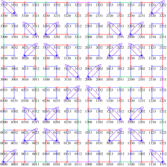
In this section we apply the result from the previous section to determine the four dimensions studied here of the generalized Sierpiński graphs , see Fig. 7 for , , and .

Let and let be a fixed integer. Then, by the definition of the generalized Sierpiński graphs , the vertex set partitions into subsets , , where the vertices of start with . That is, , where we use the convention that if is a set of strings, then is the set of strings derived by prefixing in each string from . Moreover, for , the induced subgraphs are isometric subgraphs of and are isomorphic to .
Theorem 4.1.
If , then the following hold.
-
(i)
.
-
(ii)
.
Proof.
Let and for set
The first three of these sets are thus
while the vertices from the set are marked in Fig. 8.
We claim that is a resolving set of and proceed by induction on . Since and , the claim holds true for . We can also easily verify directly that the claim is true for . So it remains to verify that , , is a resolving set of . Consider arbitrary vertices and of .
Assume first that . When and , then for . Similarly, when and , then for . Also, if , then and if , then satisfies the inequality . We can conclude that if , then the vertices and are resolved by .
Assume second that . We may without loss of generality assume that . By the induction assumption and the structure of , the set resolves . By the construction, and . Thus . However, and for every . We can thus conclude that is a resolving set of .
If , then clearly . Resolving this recurrence relation we get for . Thus, . On the other hand, using induction we infer that a vertex of , where , is a twin vertex if and only if its degree is and lies in a 4-cycle containing another vertex of degree (which is the twin of ). Moreover, each twin set is of cardinality and contains exactly one vertex of ; see Fig. 8 again. Hence by Proposition 3.1(i) we have , hence we may conclude that . From here, and recalling the fact that each twin set is of cardinality , Proposition 3.1(iii) yields .
5 Comparison and Future Direction
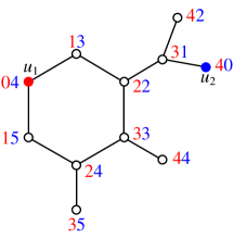
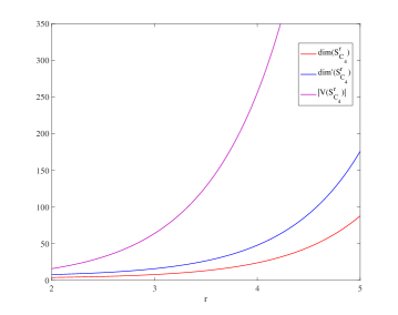
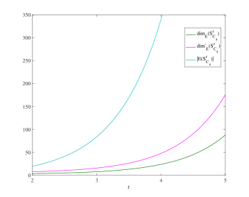
Assignment of tasks to efficient labour gives rise to yet another problem of job allocation. When a person is not able to perform the task assigned to him, it is very difficult to identify an efficient and equivalent skilful person to complete the task. This is sometimes easy if all of them are equally trained. Let us consider the situation of basis in a complete graph. If an element of the basis of a complete graph becomes faulty, then the node outside the basis can perform the task of the faulty one. This happens due to the availability of the node outside the basis. But, in general, we cannot expect this to happen on any basis of an arbitrary graph. On the other side of the problem, if one node of the basis is faulty, then precisely one node that is the best replacement for that node exists. If this happens for every member of the basis, then the fault-tolerant basis is twice that of the basis. This may motivate us to conclude . But in reality, this is not true. Fig. 9 shows a graph with . It is clear from the figure that the node and node best replace each other whereas for the node we require and as the replacement nodes. Characterization of graphs which admits were reported in [2] and the authors proved that this holds for a certain fractal cubic network. This paper investigates yet another graph class for which . The graphical comparison on , and over the node set cardinality is depicted in Fig. 10(a). Similarly for and over the edge set cardinality is depicted in Fig. 10(b).
6 Conclusion
The metric dimension of a graph is a measure of how many vertices (or nodes) are needed to uniquely identify all other vertices in the graph based on distance information. By identifying a small set of nodes that can uniquely identify all other nodes in the network, routing algorithms can be optimized to minimize message overhead and latency. By studying the metric dimension, researchers can analyze the network’s resilience to node or link failures and develop strategies for fault recovery and rerouting in parallel computing systems. Insights gained from studying the metric dimension of a network can provide valuable insights into the network’s characteristics and behavior, which can be leveraged to optimize routing algorithms, and enhance overall performance in parallel computing systems. In some cases, sensors may be placed in the nodes of a parallel computing network for various purposes, depending on the specific requirements of the application and the goals of the system. In this paper, the metric dimension, edge metric dimension and their fault-tolerant versions are investigated for the generalized Sierpiński graphs derived from . This family of graphs have an intresting relation with the widely known interconnection network, hypercube. The -dimensional generalized Sierpiński graph is a spanning subgraph of the dimensional hypercube.
Acknowledgements
Sandi Klavžar was supported by the Slovenian Research Agency ARIS (research core funding P1-0297 and projects J1-2452, N1-0285).
References
- [1] R. Alfarisi, L. Susilowati, D. Dafik and S. Prabhu, Local multiset dimension of amalgamation graphs, F1000Research 12 (2023) 95.
- [2] M. Arulperumjothi, S. Klavžar and S. Prabhu, Redefining fractal cubic networks and determining their metric dimension and fault-tolerant metric dimension, Applied Mathematics and Computation 452 (2023) 128037.
- [3] K. Balakrishnan, M. Changat, A.M. Hinz and D.S. Lekha, The median of Sierpiński graphs, Discrete Applied Mathematics 319 (2022) 159–170.
- [4] M. Basak, L. Saha, G.K. Das and K. Tiwary, Fault-tolerant metric dimension of circulant graphs , Theoretical Computer Science 817 (2020) 66–79.
- [5] Z. Beerliova, F. Eberhard, T. Erlebach, A. Hall, M. Hoffmann, M. Mihal’ák and L.S. Ram, Network discovery and verification, IEEE Journal on Selected Areas in Communications 24 (2006) 2168–2181.
- [6] A. Borodin and J.E. Hopcroft, Routing, merging and sorting on parallel models of computation, STOC ’82: Proceedings of the fourteenth annual ACM symposium on Theory of computing (1982) 338–344.
- [7] G. Chartrand, L. Eroh, M.A. Johnson and O.R. Oellermann, Resolvability in graphs and the metric dimension of a graph, Discrete Applied Mathematics 105 (2000) 99–113.
- [8] G. Chartrand and P. Zhang, The theory and applications of resolvability in graphs, a survey, Congressus Numerantium 160 (2003) 47–68.
- [9] M.C. Chen, A design methodology for synthesizing parallel algorithms and architectures, Journal of Parallel and Distributed Computing 3(4) (1986) 461–491.
- [10] T.Y. Cheung, Graph traversal techniques and the maximum flow problem in distributed computation, IEEE Transactions on Software Engineering SE-9(4) (1983) 504–512.
- [11] P.J. Cleall, H.R. Thomas, T.A. Melhuish and D.H. Owen, Use of parallel computing and visualisation techniques in the simulation of large scale geoenvironmental engineering problems, Future Generation Computer Systems 22(4) (2006) 460–467.
- [12] V.J.A. Cynthia, M. Ramya and S. Prabhu, Local metric dimension of certain classes of circulant networks, Journal of Advanced Computational Intelligence and Intelligent Informatics 27(4) (2023) 554–560.
- [13] R. Duncan, A survey of parallel computer architectures, Computer 23(2) (1990) 5–16.
- [14] W.M. Eddy and M. Allman, Advantages of parallel processing and the effects of communications time, (2000) No. NASA/CR-2000-209455.
- [15] E. Estaji and J.A. Rodríguez-Velázquez, The strong metric dimension of generalized Sierpiński graphs with pendant vertices, Ars Mathematica Contemporanea 12 (2017) 127–134.
- [16] A. Estrada-Moreno and J.A. Rodríguez-Velázquez, On the general randić index of polymeric networks modelled by generalized Sierpiński graphs, Discrete Applied Mathematics 263 (2019) 140–151.
- [17] E. Fernández and H.F. Jelinek, Use of fractal theory in neuroscience: Methods, advantages, and potential problems, Methods 24(4) (2001) 309–321.
- [18] S. Gravier, M. Kovše and A. Parreau, Generalized Sierpiński graphs, in: EuroComb 2011 (Poster), Rényi Institute, Budapest page URL http://www.renyi.hu/conferences/ec11/posters/parreau.pdf, 2011.
- [19] F. Harary and R.A. Melter, On the metric dimension of a graph, Ars Combinatoria 2 (1976) 191–195.
- [20] C. Hernando, M. Mora, I.M. Pelayo, C. Seara and D.R. Wood, Extremal graph theory for metric dimension and diameter, Electronic Journal of Combinatorics 17 (2010) R30.
- [21] C. Hernando, M. Mora, P.J. Slater and D.R. Wood, Fault-tolerant metric dimension of graphs, Convexity in Discrete Structures 5 (2008) 81–85.
- [22] A.M. Hinz and C.H. auf der Heide, An efficient algorithm to determine all shortest paths in Sierpiński graphs, Discrete Applied Mathematics 177 (2014) 111–120.
- [23] A.M. Hinz, S. Klavžar and S.S. Zemljič, A survey and classification of Sierpiński-type graphs, Discrete Applied Mathematics 217 (2017) 565–600.
- [24] A.M. Hinz and D. Parisse, The average eccentricity of Sierpiński graphs, Graphs and Combinatorics 28(5) (2012) 671–686.
- [25] M. Imran, Sabeel-e-Hafi, W. Gao and M.R. Farahani, On topological properties of Sierpiński networks, Chaos, Solitons & Fractals 98 (2017) 199–204.
- [26] M. Johnson, Structure-activity maps for visualizing the graph variables arising in drug design, Journal of Biopharmaceutical Statistics 3(2) (1993) 203–236.
- [27] A. Kelenc, N. Tratnik and I.G. Yero, Uniquely identifying the edges of a graph: The edge metric dimension, Discrete Applied Mathematics 251 (2018) 204–220.
- [28] A. Kelenc, A.T.M. Toshi, R. Škrekovski and I.G. Yero, On metric dimensions of hypercubes, Ars Mathematica Contemporanea 23(2) (2022) P2.08.
- [29] S. Khuller, J.B. Raghavachari and A. Rosenfeld, Landmarks in graphs, Discrete Applied Mathematics 70(3) (1996) 217–229.
- [30] S. Klavžar and D. Kuziak, Nonlocal metric dimension of graphs, Bulletin of the Malaysian Mathematical Sciences Society 46 (2023) 66.
- [31] S. Klavžar and U. Milutinović, Graphs and a variant of the tower of Hanoi problem, Czechoslovak Mathematical Journal 47(1) (1997) 95–104.
- [32] S. Klavžar and M. Tavakoli, Edge metric dimensions via hierarchical product and integer linear programming, Optimization Letters 15 (2021) 1993–2003.
- [33] S. Klavžar and S.S. Zemljič, On distances in Sierpiński graphs: Almost-extreme vertices and metric dimension, Applicable Analysis and Discrete Mathematics 7 (2013) 72–82.
- [34] S. Klavžar and S.S. Zemljič, Connectivity and some other properties of generalized Sierpiński graphs, Applicable Analysis and Discrete Mathematics 12(2) (2018) 401–412.
- [35] M. Knor, S. Majstorović, A.T.M. Toshi, R. Škrekovski and I.G. Yero, Graphs with the edge metric dimension smaller than the metric dimension, Applied Mathematics and Computation 401 (2021) 126076.
- [36] M. Knor, R. Škrekovski and I.G. Yero, A note on the metric and edge metric dimensions of 2-connected graphs, Discrete Applied Mathematics 319 (2022) 454–460.
- [37] K. Liu and N. Abu-Ghazaleh, Virtual coordinates with backtracking for void traversal in geographic routing, ADHOC-NOW 2006, Lecture Notes in Computer Science 4104 (2006) 45–59.
- [38] O. López-Ortega and S.I. López-Popa, Fractals, fuzzy logic and expert systems to assist in the construction of musical pieces, Expert Systems with Applications 39(15) (2012) 11911–11923.
- [39] D. Lüdtke and D. Tutsch, The modeling power of CINSim: Performance evaluation of interconnection networks, Computer Networks 53 (2009) 1274–1288.
- [40] P. Manuel, B. Rajan, I. Rajasingh and M.C. Monica, On minimum metric dimension of honeycomb networks, Journal of Discrete Algorithms 6 (2008) 20–27.
- [41] P.D. Manuel, M.I. Abd-El-Barr, I. Rajasingh and B. Rajan, An efficient representation of benes networks and its applications, Journal of Discrete Algorithms 6(1) (2008) 11–19.
- [42] R.P. Martin, A.M. Vahdat, D.E. Culler and T.E. Anderson, Effects of communication latency, overhead, and bandwidth in a cluster architecture, ACM SIGARCH Computer Architecture News 25(2) (1997) 85–97.
- [43] R.A. Melter and I. Tomescu, Metric bases in digital geometry, Computer Vision, Graphics, and Image Processing 25(1) (1984) 113–121.
- [44] M. Obert, P. Pfeifer and M. Sernetz, Microbial growth patterns described by fractal geometry, Journal of Bacteriology 172(3) (1990) 1180–1185.
- [45] I. Peterin and I.G. Yero, Edge metric dimension of some graph operations, Bulletin of the Malaysian Mathematical Sciences Society 43 (2020) 2465–2477.
- [46] S. Prabhu, T. Flora and M. Arulperumjothi, On independent resolving number of TiO nanotubes, Journal of Intelligent & Fuzzy Systems 35(6) (2018) 6421–6425.
- [47] S. Prabhu, D.S.R. Jeba, M. Arulperumjothi and S. Klavžar, Metric Dimension of Irregular Convex Triangular Networks, AKCE International Journal of Graphs and Combinatorics (2023) DOI: 10.1080/09728600.2023.2280799.
- [48] S. Prabhu, V. Manimozhi, M. Arulperumjothi and S. Klavžar, Twin vertices in fault-tolerant metric sets and fault-tolerant metric dimension of multistage interconnection networks, Applied Mathematics and Computation 420 (2022) 126897.
- [49] B. Rajan, I. Rajasingh, J.A. Cynthia and P. Manuel, Metric dimension of directed graphs, International Journal of Computer Mathematics 91(7) (2014) 1397–1406.
- [50] F. Ramezani, E.D. Rodríquez-Bazan and J.A. Rodríguez-Velázquez, On the roman domination number of generalized Sierpiński graphs, Filomat 31(20) (2017) 6515–6528.
- [51] H. Raza, S. Hayat and X.F. Pan, On the fault-tolerant metric dimension of certain interconnection networks, Journal of Applied Mathematics and Computing 60 (2019) 517–535.
- [52] J.A. Rodríguez-Velázquez, E.D. Rodríquez-Bazan and A. Estrada-Moreno, On generalized Sierpiński graphs, Discussiones Mathematicae Graph Theory 37(3) (2017) 547–560.
- [53] P.J. Slater, Leaves of trees, Congressus Numerantium 14 (1975) 549–559.
- [54] R.C. Tillquist, R.M. Frongillo and M.E. Lladser, Getting the lay of the land in discrete space: A survey of metric dimension and its applications, SIAM Review 65(4) (2023) 919–962.
- [55] G.D. Vecchia and C. Sanges, A recursively scalable network VLSI implementation, Future Generation Computer Systems 4(5) (1988) 235–243.
- [56] D.G.L. Wang, M.M.Y. Wang and S. Zhang, Determining the edge metric dimension of the generalized Petersen graph , Journal of Combinatorial Optimization 43 (2022) 460–496.
- [57] C. Wei, M. Salman, S. Shahzaib, M.U. Rehman and J. Fang, Classes of planar graphs with constant edge metric dimension, Complexity 2021 (2021) 5599274.
- [58] Y. Zhang and S. Gao, On the edge metric dimension of convex polytopes and its related graphs, Journal of Combinatorial Optimization 39 (2020) 334–350.
- [59] E. Zhu, A. Taranenko, Z. Shao and J. Xu, On graphs with the maximum edge metric dimension, Discrete Applied Mathematics 257 (2019) 317–324.
- [60] N. Zublirina, Asymptotic behavior of the edge metric dimension of the random graph, Discussiones Mathematicae Graph Theory 41(2) (2021) 589–599.
- [61] N. Zubrilina, On the edge dimension of a graph, Discrete Mathematics 341 (2018) 2083–2088.