Cosmological singularities,
holographic complexity and entanglement

K. Narayan,  Hitesh K. Saini,  Gopal Yadav

Chennai Mathematical Institute,
H1 SIPCOT IT Park, Siruseri 603103, India.

We study holographic volume complexity for various families of holographic cosmologies with Kasner-like singularities, in particular with $AdS$, hyperscaling violating and Lifshitz asymptotics. We find through extensive numerical studies that the complexity surface always bends in the direction away from the singularity and transitions from spacelike near the boundary to lightlike in the interior. As the boundary anchoring time slice approaches the singularity, the transition to lightlike is more rapid, with the spacelike part shrinking. The complexity functional has vanishing contributions from the lightlike region so in the vicinity of the singularity, complexity is vanishingly small, indicating a dual Kasner state of vanishingly low complexity, suggesting an extreme thinning of the effective degrees of freedom dual to the near singularity region. We also develop further previous studies on extremal surfaces for holographic entanglement entropy, and find that in the IR limit they reveal similar behaviour as complexity.

1 Introduction

Among the various quantum information ideas and tools that have become ubiquitous in holography over the last several years, a fascinating class of questions involves computational complexity. Complexity measures the difficulty in preparation of the final state from some initial reference state. Discussions of eternal black holes dual to thermofield double states and ER=EPR [2] suggested that the linear growth in time of the spatial volume of the bulk Einstein-Rosen bridge is dual to the linear time growth of complexity in the dual field theory [3, 4, 5, 6, 7]. This is encapsulated in the expression

$$C(t)\sim{{\rm Vol}(\Sigma_{t})\over G_{N}R}\,,$$ (1.1)

for complexity $C(t)$ in terms of an extremal codim-1 spacelike slice $\Sigma_{t}$ at anchoring time $t$, with $G_{N}$ the Newton constant in $AdS$ with scale $R$. The precise proportionality factors are not canonical to pin down and are likely detail-dependent. In time-independent cases, the extremal codim-1 surface volumes have dominant contributions from the near boundary region (with cutoff $\epsilon$ and $d_{i}$ spatial dimensions), giving the scaling $C(t)\propto{R^{d_{i}+1}\over G_{d_{i}+2}\,R}\,{V_{d_{i}}\over\epsilon^{d_{i}}}\equiv N_{dof}\,V_{d_{i}}\Lambda_{{}_{UV}}^{d_{i}}$ . This reflects the fact that complexity scales with the number of degrees of freedom in the dual field theory and with spatial volume in units of the UV cutoff. Extensive further investigations of holographic complexity including other proposals (such as complexity-equals-action, complexity-equals-anything, path integral complexity), in particular with relevance to cosmological contexts, appear in e.g. [8]-[75] (see also the review [76]).

It is fascinating to use such quantum information tools to probe cosmological singularities which remain mysterious in many ways: we will employ the “complexity equals volume” proposal (1.1) in this regard. One might expect severe stringy and quantum effects to be important here. In the context of holography, one might imagine certain classes of severe time-dependent deformations of the CFT to be useful in shedding light on Big Bang/Crunch singularities. A prototypical example is the $AdS_{5}$ Kasner background, where the dual Super Yang-Mills CFT can be regarded as subjected to severe time dependent deformations (of the gauge coupling and the space on which the CFT lives) [77, 78, 79, 80]; see also [81, 82, 83, 84] (and [85, 86] for some reviews pertaining to Big-Bang/Crunch singularities and string theory). These are likely to be qualitatively different from bulk black holes however, which being dual to thermal states might be regarded as natural endpoints for generic time-dependent perturbations that would thermalize on long timescales. There are indications that the dual state to a Big-Bang/Crunch is quite non-generic. For instance, volume complexity for $AdS$-Kasner singularities was found to become vanishingly low in [11] (see also [54]). This also appears consistent with the investigations of classical and quantum codim-2 extremal surfaces and holographic entanglement entropy in $AdS$ Kasner and other singularities [87], [88]: the entangling surfaces are driven away from the near singularity region (for spacelike singularities). These results suggest that the effective number of qubits dual to the near singularity region is vanishingly small, giving low complexity for the “dual Kasner state” independent of the reference state, and low entanglement. The bulk singularity is a Big-Bang/Crunch where spatial volumes, and thus the number of degrees of freedom, become vanishingly small. In some ways this might naively contrast with colloquial thinking that a Big-Bang singularity is a “hot dense mess” (e.g. in FRW cosmologies) but perhaps reflects the fact that these holographic singularities are low entropy configurations. Note also that in the eternal $AdS$ black hole, the complexity extremal surfaces slice through the interior but stay well away from the black hole singularity, approaching a limiting surface for late times $t\rightarrow\infty$ (analogous to [89] for holographic entanglement entropy [90, 91, 92, 93]). This appears to dovetail with the above, recalling the fact that the black hole interior is a cosmology with a spacelike Big-Crunch singularity.

In the present paper we build on some of these investigations and study holographic complexity and entanglement. Paraphrasing from sec. 3.1.1 and sec. 3.4, we find that the codim-1 complexity extremal surface anchored at some boundary time slice $t$ some finite temporal distance from the singularity at $t=0$ begins as a spacelike surface near the boundary, bends away from the singularity and approaches a lightlike trajectory in the $(t,r$)-plane with $r$ the bulk holographic direction. As the anchoring time slice $t$ becomes smaller, i.e. going towards the singularity, the surface transitions more quickly from spacelike towards the lightlike limit. These features are depicted qualitatively in Fig. 15. The lightlike part has vanishing volume so the complexity volume functional becomes small as $t$ becomes small and eventually becomes vanishingly small as $t\rightarrow 0$ towards the singularity. This behaviour is universal for various classes of Big-Bang/Crunch singularities, viz. $AdS$ Kasner, hyperscaling violating Kasner and Lifshitz Kasner. For $AdS$-Kasner and Lifshitz-Kasner backgrounds, complexity decreases linearly with the anchoring boundary time slice $t$ as $t\rightarrow 0$. For the hyperscaling violating Kasner backgrounds, the complexity decrease is not linear with time $t$, reflecting the nontrivial effective spatial dimension of the dual field theories. Overall our results on complexity corroborate the discussions on complexity for $AdS$ Kasner in [11] but our analysis, especially the extensive numerical studies, hopefully adds somewhat greater detail. The complexity results for other cosmologies we discuss are new but in accord with those for $AdS$ Kasner.

Our technical analysis for complexity has several parallels with that in [87] of holographic entanglement entropy [90, 91, 92, 93], in the semiclassical region far from the singularity. Here we extend that analysis numerically along the lines of volume complexity above for entanglement as well. The codim-2 area functional has many technical similarities with the codim-1 volume complexity functional so we find similar results in the IR limit when the subregions are large and essentially cover the whole space. The surface transitions from spacelike near the boundary to lightlike in the interior. As the anchoring time slice $t$ approaches the singularity, the lightlike transition is more rapid. As $t\rightarrow 0$, the entanglement entropy becomes vanishingly small.

The vanishingly low complexity (and entanglement) for times approaching the singularity reflect the fact that spatial volumes Crunch there, so the effective number of degrees of freedom near the singularity is vanishingly small. From the point of view of constructing the dual “Kasner” state from some reference state, it appears that there are simply vanishingly small numbers of effective qubits in the vicinity of the singularity, independent of any reference initial state, thus leading to low complexity.

The cosmological backgrounds are mostly isotropic, so the resulting complexity volume functional can be recast in an effective 2-dimensional form, consistent with dimensional reduction of all the boundary spatial dimensions. This results in a relatively simple expression for complexity solely in terms of the variables describing the effective 2-dim dilaton gravity theory arising under reduction, i.e. the 2-dim metric and the dilaton (which is the higher dimensional transverse area). It may be interesting to interpret this effective 2-dimensional holographic complexity in terms of appropriate dual effective 1-dim qubit models.

This paper is organized as follows. In sec. 2, we argue that volume complexity in these higher-dimensional theories can be compactly recast as complexity in effective 2-dim theories that can be regarded as arising by dimensional reduction. In sec. 3, we discuss holographic complexity of $AdS$-Kasner: in sec. 3.1, sec. 3.2, and sec. 3.3, we obtain the solution of the equations of motion associated with complexity surfaces for AdS_5,4,7-Kasner spacetimes which we then use to obtain the holographic complexity of AdS_5,4,7-Kasner spacetimes numerically in sec. 3.4. Sec. 4 discusses holographic complexity in hyperscaling violating cosmologies, focussing on $d_{i}=2,\ \theta=-{1\over 3}$ (sec. 4.1) and $d_{i}=4,\ \theta=-1$ (sec. 4.2): we then numerically compute holographic complexity in these cosmologies in sec. 4.3. In sec. 5, we compute the holographic complexity of isotropic Lifshitz Kasner cosmology. We review aspects of the holographic entanglement studies in [87] in sec. 6. We use this to discuss the behavior of RT/HRT surfaces for $AdS$-Kasner spacetime in sec. 7 via sec. 7.1 ($AdS_{5}$-Kasner) and sec. 7.2 ($AdS_{7}$-Kasner) and then compute holographic entanglement entropy numerically in sec. 7.3 of $AdS_{5,7}$-Kasner spacetimes. Sec. 8 contains a Discussion of our results alongwith various comments and questions.

In App. A, we briefly review earlier studies on holographic cosmologies and their 2-dim reduction and in App. B, we have listed the coefficients appearing in the perturbative solution of AdS-Kasner and hyperscaling violating cosmologies. In App. C, we briefly discuss our numerical methods applied to entanglement for finite subregions, with the results vindicating expectations and thereby our overall analysis.

2 ​​​ Higher dim volume complexity​ $\rightarrow$ 2-dims: generalities

The metric for an eternal $AdS_{d_{i}+2}$ Schwarzschild black hole (with transverse space $d\sigma_{d_{i}}^{2}$) is

$$ds^{2}={R^{2}\over r^{2}}\Big{(}-H(r)dt^{2}+{dr^{2}\over H(r)}+d\sigma_{d_{i}}^{2}\Big{)}\,.$$ (2.1)

Then the complexity volume functional given by the volume of the Einstein-Rosen bridge is

$$C_{D}={V_{d_{i}}\over G_{d_{i}+2}R}\int dr{R^{d_{i}+1}\over r^{d_{i}+1}}\sqrt{{1\over H(r)}-H(r)t^{\prime}(r)^{2}}\,.$$ (2.2)

Since the transverse space (that the codim-1 extremal surface wraps) appears in a simple way in this expression, the complexity functional is effectively 2-dimensional and can be recast explicitly in terms of the complexity of an effective 2-dim dilaton gravity theory obtained by dimensional reduction over the transverse space $d\sigma_{d_{i}}^{2}$. This is quite general and applies for large families of backgrounds that are “mostly” isotropic: the 2-dim dilaton gravity theory for various purposes encapsulates the higher dimensional gravity theory [94]. We will find this perspective useful in what follows, where we study holographic backgrounds containing cosmological singularities, particularly those studied in [95]. A brief review of these studies and holographic cosmologies appears in App. A.

Consider the general ansatz for a $D=d_{i}+2$ dimensional gravity background

$$ds_{D}^{2}=g_{\mu\nu}^{(2)}dx^{\mu}dx^{\nu}+\phi^{2/d_{i}}d\sigma_{d_{i}}^{2}=\frac{e^{f}}{\phi^{(d_{i}-1)/d_{i}}}(-dt^{2}+dr^{2})+\phi^{2/d_{i}}d\sigma_{d_{i}}^{2}\,,$$

$$ds^{2}=g_{\mu\nu}dx^{\mu}dx^{\nu}=e^{f}\,(-dt^{2}+dr^{2})\,,\qquad g_{\mu\nu}=\phi^{(d_{i}-1)/d_{i}}g_{\mu\nu}^{(2)}\,.$$ (2.3)

Reviewing [94], [95], performing dimensional reduction over the transverse space $d\sigma_{d_{i}}^{2}$ gives rise to a 2-dim dilaton gravity theory. With the above parametrization, the higher dimensional transverse area is the 2-dim dilaton $\phi$. The Weyl transformation $g_{\mu\nu}=\phi^{(d_{i}-1)/d_{i}}g^{(2)}_{\mu\nu}$ absorbs the dilaton kinetic energy into the curvature $R^{(2)}$ and the 2-dim action becomes

$$S={1\over 16\pi G_{2}}\int d^{2}x\sqrt{-g}\left(\phi{\cal R}-U(\phi,\Psi)-{1\over 2}\,\phi(\partial\Psi)^{2}\right),$$ (2.4)

with the dilaton potential $U(\phi,\Psi)$ potentially coupling $\phi$ to another scalar $\Psi$ which is a minimal massless scalar in the higher dimensional theory (see App. A). The dilaton factor in the $\Psi$ kinetic energy arises from the reduction to 2-dimensions. These models with various kinds of dilaton potentials encapsulate large families of nontrivial higher dimensional gravity theories with spacelike Big-Bang/Crunch type cosmological singularities. In the vicinity of the singularity, the 2-dim fields have power-law scaling behaviour of the form (setting dimensionful scales to unity)

$$\phi=t^{k}r^{m}\,,\qquad e^{f}=t^{a}r^{b}\,,\qquad e^{\Psi}=t^{\alpha}r^{\beta}\,,$$ (2.5)

and the forms of $e^{f},\phi$ then translate to the higher dimensional cosmological background profile containing the singularities. The 2-dim formulation leads to various simplifications in the structure of these backgrounds and reveals certain noteworthy features. In particular, the severe time-dependence in the vicinity of the singularity implies that the time derivative terms are dominant while other terms, in particular pertaining to the dilaton potential, are irrelevant there. This then reveals a “universal” subsector with $k=1$,

$$\phi\sim t\,,\qquad e^{f}\sim t^{a}\,,\qquad e^{\Psi}\sim t^{\alpha}\,;\qquad\quad a={\alpha^{2}\over 2}\,.$$ (2.6)

A prototypical example is $AdS$ Kasner [77] and its reduction to 2-dimensions,

$$ds^{2}={R^{2}\over r^{2}}(-dt^{2}+dr^{2})+{t^{2/d_{i}}\,R^{2}\over r^{2}}dx_{i}^{2}\,,\qquad e^{\Psi}=t^{\sqrt{{2(d_{i}-1)/d_{i}}}}\,,\qquad\Lambda=-{d_{i}(d_{i}+1)\over 2R^{2}}\,,\quad$$

$$\rightarrow \qquad\ \phi={t\,R^{d_{i}}\over r^{d_{i}}}\,,\qquad ds^{2}={t^{(d_{i}-1)/d_{i}}\,R^{d_{i}+1}\over r^{d_{i}+1}}(-dt^{2}+dr^{2})\,,\qquad U=2\Lambda\phi^{1/d_{i}}\,.$$ (2.7)

The isotropic restriction from general $AdS$ Kasner (A1) alongwith the Kasner exponent relation $\sum_{i}p_{i}=1$ implies a single Kasner exponent $p={1\over d_{i}}$. $R$ is the $AdS$ length scale. We are suppressing an implicit Kasner scale $t_{K}$: e.g. $t^{2p}\rightarrow(t/t_{K})^{2p}$. We will reinstate this as required. There are several more general families of such backgrounds with Big-Bang/Crunch singularities, including nonrelativistic ones such as hyperscaling violating (conformally $AdS$) theories, and those with nontrivial Lifshitz scaling, as we will discuss in what follows, and summarized in the Table 1.

Cosmologies	$k$	$m$	$a={\alpha^{2}\over 2}$	$b$
$AdS$ Kasner cosmology	1	$-d_{i}$	$\frac{d_{i}-1}{d_{i}}$	$-(d_{i}+1)$
Hv cosmology ($z=1,\ \theta\neq 0$)	1	$-(d_{i}-\theta)$	$\left(\sqrt{\frac{d_{i}-\theta-1}{d_{i}-\theta}}-\sqrt{\frac{(-\theta)}{d_{i}(d_{i}-\theta)}}\right)^{2}$	$-\frac{(d_{i}-\theta)(1+d_{i})}{d_{i}}$
Lif cosmology ($z=d_{i},\ \theta=0$)	1	$-1$	${d_{i}-1\over d_{i}}$	$-3+{1\over d_{i}}$

Table 1: Exponents for 2-dim cosmologies.

The time dependence in these backgrounds does not switch off asymptotically so that simple interpretations in terms of deformations of some vacuum state appear difficult: instead these are probably best regarded as dual to some nontrivial nongeneric state in the dual field theory. This is consistent with the expectation that generic severe time-dependent CFT deformations will thermalize and thus be dual to black hole formation in the bulk. Further discussions on this perspective appear throughout the paper (building on [77, 78, 79, 80], and [87], [88]).

We now come to complexity. We mostly consider the transverse space to be planar, so $d\sigma_{d_{i}}^{2}=\sum_{i}dx_{i}^{2}$. Then, in terms of 2-dim variables (2) the complexity volume functional becomes

$$C = {1\over G_{d_{i}+2}R}\int\prod_{j=1}^{d_{i}}\left(\phi^{1/d_{i}}dx_{j}\right)\sqrt{\frac{e^{f}}{\phi^{(d_{i}-1)/d_{i}}}(-dt^{2}+dr^{2})}$$ (2.8)

$$= {V_{d_{i}}\over G_{d_{i}+2}R}\int_{\epsilon}dr\ \phi^{\frac{(d_{i}+1)}{2d_{i}}}\,e^{f/2}\,\sqrt{1-t^{\prime}(r)^{2}}\ =\ {1\over G_{2}R}\int_{\epsilon}dr\ \phi^{\frac{(d_{i}+1)}{2d_{i}}}\,e^{f/2}\,\sqrt{1-t^{\prime}(r)^{2}}\,,\qquad$$

with $G_{2}={G_{d_{i}+2}\over V_{d_{i}}}$ the 2-dimensional Newton constant after reduction, and $r=\epsilon$ the holographic boundary. The higher dimensional curvature scale (e.g. $R$ in (2)) continues as the 2-dim curvature scale. Also, $t^{\prime}\equiv{dt\over dr}$ is the $r$-derivative of the time coordinate as a function $t(r)$ of the holographic radial coordinate.

The last expression in (2.8) above can be interpreted as the complexity volume functional in the 2-dim dilaton gravity theory intrinsically. It would then be interesting to ask for dual 1-dimensional effective qubit models whose complexity can be understood as this.

Sticking in the power-law ansatze (2.5) above, we obtain

$$C=\frac{V_{d_{i}}}{G_{d_{i}+2}R}\int_{\epsilon}dr\,\ t(r)^{\left(k\left(\frac{(d_{i}+1)}{2d_{i}}\right)+\frac{a}{2}\right)}\ r^{\left(m\left(\frac{(d_{i}+1)}{2d_{i}}\right)+\frac{b}{2}\right)}\ \sqrt{1-t^{\prime}(r)^{2}}\ \equiv\ \frac{V_{d_{i}}}{G_{d_{i}+2}R}\int_{\epsilon}dr\,{\cal L}\,,$$ (2.9)

with ${\cal L}\equiv{\cal L}\left(r,t(r),t^{\prime}(r)\right)$ the effective Lagrangian. Extremizing for the complexity surface $t(r)$ leads to the Euler-Lagrange equation $\frac{d}{dr}\big{(}\frac{\partial{\cal L}}{\partial t^{\prime}(r)}\big{)}-\frac{\partial{\cal L}}{\partial t(r)}=0$ .  Simplifying this gives the equation of motion for the complexity surface $t(r)$ in (2.9)

$$2d_{i}r\,t\,t^{\prime\prime}+r\,(ad_{i}+d_{i}+1)\,\left(1-(t^{\prime})^{2}\right)+(bd_{i}+d_{i}m+m)\,t\,t^{\prime}\left(1-(t^{\prime})^{2}\right)=0\,,$$ (2.10)

abbreviating notation with $t\equiv t(r),\ t^{\prime}\equiv{dt\over dr}\,,\ t^{\prime\prime}\equiv{d^{2}t\over dr^{2}}$, and we have used the universality result $k=1$ in (2.6).

Now we solve equation (2.10) perturbatively and numerically for $AdS$ Kasner, hyperscaling violating and Lifshitz cosmologies, and thereby compute holographic complexity for these cosmologies in sections 3 and 4.

Methodology: We outline our techniques and methods here:

1. For a given background, first, we solve (2.10) semiclassically in perturbation theory using an ansatz of the form $t(r)=\sum_{n\in\mathbb{Z}_{+}}c_{n}r^{n}$ for the complexity surfaces $t(r)$, as functions of the radial coordinate $r$ for various anchoring time slices $t_{0}$ which define boundary conditions at $r=0$. The perturbative solutions are valid only in a certain $r$-regime, i.e. upto a cut-off $r_{\Lambda}$ (roughly $r_{\Lambda}\lesssim t_{0}$). Thus these cannot encapsulate the entire bulk geometry.

2. To overcome this and obtain a global picture of the bulk, we solve (2.10) numerically (in Mathematica). For this purpose, we need two initial conditions which we extract from the perturbative solutions for $t(r)$ above and their derivatives $t^{\prime}(r)$, setting the boundary value $r=\epsilon=10^{-2}$ and $t_{0}$ as the numerical value of a specific anchoring time slice (with all other dimensionful scales set to unity). This allows us to obtain numerical solutions for the complexity surfaces, which then reveal nontrivial bulk features such as lightlike limits and the transition thereto, from spacelike regimes near the boundary. This then allows us to numerically evaluate holographic volume complexity and plot it against $t_{0}$ for various backgrounds.

3. We then employ similar algorithms broadly for holographic entanglement entropy.

4. Some numerical issues persist for certain backgrounds, as we state in what follows, and we suppress detailed discussions in these cases.

3 Complexity: $AdS$ Kasner

The isotropic $AdS_{d_{i}+2}$ Kasner spacetime (2) in the form of the reduction ansatz (2) alongwith its 2-dim exponents (2.5), is:

$$ds^{2}={R^{2}\over r^{2}}(-dt^{2}+dr^{2})+{t^{2/d_{i}}\,R^{2}\over r^{2}}dx_{i}^{2}\,,\qquad e^{\Psi}=t^{\sqrt{{2(d_{i}-1)/d_{i}}}}\,,\qquad\Lambda=-{d_{i}(d_{i}+1)\over 2R^{2}}\,,\qquad$$

$$\quad\phi={t\,R^{d_{i}}\over r^{d_{i}}}\,,\qquad ds^{2}={t^{(d_{i}-1)/d_{i}}\,R^{d_{i}+1}\over r^{d_{i}+1}}(-dt^{2}+dr^{2})\,,\qquad U=2\Lambda\phi^{1/d_{i}}\,,$$

$$\qquad k=1\,,\quad\ \ m=-d_{i}\,,\quad\ \ a=\frac{d_{i}-1}{d_{i}}\,,\quad\ \ b=-(d_{i}+1)\,,\quad\ \ \alpha=\sqrt{{2(d_{i}-1)\over d_{i}}}\ .\quad$$ (3.1)

The single Kasner exponent $p={1\over d_{i}}$ arises due to the isotropic restriction in (A1). $R$ is the $AdS$ length scale. We are suppressing an implicit Kasner scale $t_{K}$: e.g. $t^{2p}\rightarrow(t/t_{K})^{2p}$.

Then the $t(r)$ extremization equation (2.10) becomes

$$r\,t(r)\,t^{\prime\prime}(r)-({d_{i}}+1)\,t(r)\,t^{\prime}(r)\,\left(1-t^{\prime}(r)^{2}\right)+r\,\left(1-t^{\prime}(r)^{2}\right)=0\,.$$ (3.2)

We discuss the solution of (3.2) for $AdS_{5,4,7}$-Kasner spacetimes in sec. 3.1, 3.2, and 3.3.

3.1 AdS₅-Kasner spacetime

For $AdS_{5}$-Kasner spacetime, we have $d_{i}=3$: then (3.2) simplifies to

$$r\,t(r)\,t^{\prime\prime}(r)-4t(r)\,t^{\prime}(r)\,\left(1-t^{\prime}(r)^{2}\right)+r\,\left(1-t^{\prime}(r)^{2}\right)=0\,.$$ (3.3)

First we note that with $t^{\prime},t^{\prime\prime}=0$, the equation above is not satisfied except for $r\sim 0$, so that $t(r)=const$ is not a solution: the surface always bends in the time direction due to the time dependence of the background. When the complexity surface $t(r)$ has weak $r$-dependence, i.e. it is almost constant with $t(r)\sim t_{0}$, we can analyze the above equation in perturbation theory in $r$, by considering the following ansatz for $t(r)$:

$$t(r)=t_{0}+\sum_{n\in\mathbb{Z}_{+}}c_{n}r^{n}\,.$$ (3.4)

Inputting this ansatz (3.4) in (3.3) and solving for the coefficients iteratively, we find the following solution up to ${\cal O}(r^{30})$:

$$\hskip-14.45377ptt(r)=t_{0}+\frac{r^{2}}{6t_{0}}-\frac{7r^{4}}{216t_{0}^{3}}+\frac{5r^{6}}{3888t_{0}^{5}}-\frac{23r^{8}}{31104t_{0}^{7}}+\frac{5671r^{10}}{125971200t_{0}^{9}}-\frac{193157r^{12}}{31744742400t_{0}^{11}}-\frac{1451389r^{14}}{571405363200t_{0}^{13}}$$

$$\hskip-14.45377pt+\frac{126271147r^{16}}{60340406353920t_{0}^{15}}-\frac{171499492421r^{18}}{211794826302259200t_{0}^{17}}+\frac{2509650528887r^{20}}{7624613746881331200t_{0}^{19}}$$

$$\hskip-14.45377pt-\frac{23544237318388621r^{22}}{213870415600021340160000t_{0}^{21}}+\frac{74037865493904302737r^{24}}{2048023099785804353372160000t_{0}^{23}}-\frac{27221138559698748551r^{26}}{2457627719742965224046592000t_{0}^{25}}$$

$$\hskip-14.45377pt+\frac{2040692465059715118445379r^{28}}{640998461863360189735832125440000t_{0}^{27}}-\frac{414120404436438180460454771r^{30}}{480748846397520142301874094080000000t_{0}^{29}}\,.$$ (3.5)

The solution $t(r)$ in (3.1) and its derivative $t^{\prime}(r)$ are plotted in Fig. 1 for various $t_{0}$-values.

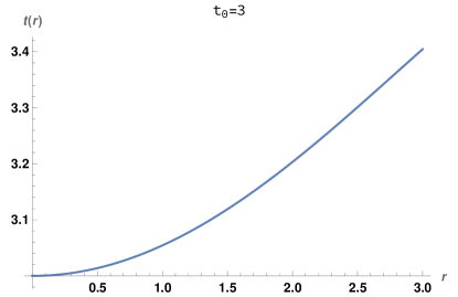
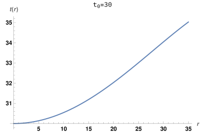
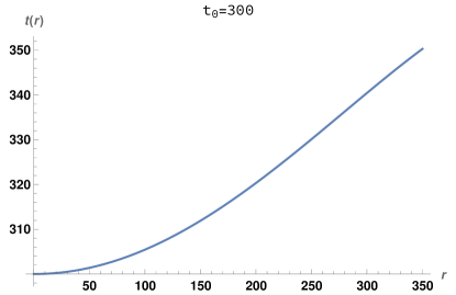
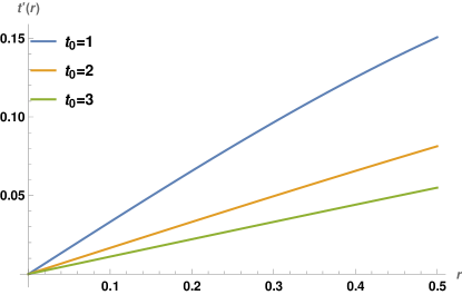
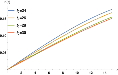
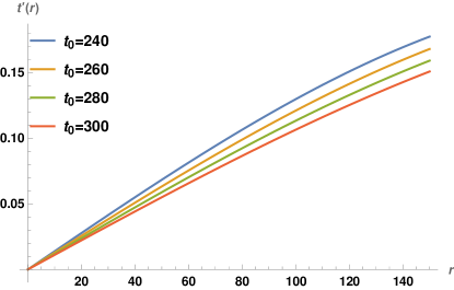
Figure 1: Variation with $r$ of the semiclassical (perturbative) complexity surfaces $t(r)$ and their derivatives $t^{\prime}(r)$ for various values of the anchoring time slice $t_{0}$.

From Fig. 1, we see that the complexity surface varies approximately linearly with $r$ in the regime roughly $r\sim t_{0}$ and $t^{\prime}(r)$ reaches its maximum value about $t^{\prime}(r)\lesssim 0.2$, which vindicates the mild bending of the surface $t(r)$ in the radial direction. Of course this perturbative solution has clear limitations, expressed as it is here by a finite power series. However it is of great value to display the behaviour of the complexity surface near the boundary $r=0$.

We expect that when the anchoring time slice $t_{0}$ is far from the singularity at $t=0$, the above perturbative solution is reasonable, at least in the neighbourhood of the boundary. A very similar analysis was carried out in [87] to reveal the RT/HRT surface in the semiclassical regime far from the singularity bends away from the singularity. We will study this numerically later revealing more information.

A further check of the above series solution is that in the semiclassical limit, when we ignore the higher order terms in $t^{\prime}(r)$ (i.e. $t^{\prime}(r)\ll 1$), then (3.3) reduces to

$$t(r)\left(rt^{\prime\prime}(r)-4t^{\prime}(r)\right)+r=0\,.$$ (3.6)

Solving (3.6) with the ansatz (3.4), we obtain up to ${\cal O}(r^{30})$:

$$\hskip-14.45377ptt(r)=t_{0}+\frac{r^{2}}{6t_{0}}-\frac{r^{4}}{24t_{0}^{3}}-\frac{5r^{6}}{432t_{0}^{5}}+\frac{r^{8}}{3456t_{0}^{7}}-\frac{19r^{10}}{518400t_{0}^{9}}-\frac{457r^{12}}{130636800t_{0}^{11}}+\frac{9889r^{14}}{16460236800t_{0}^{13}}-\frac{162763r^{16}}{579400335360t_{0}^{15}}$$

$$\hskip-14.45377pt+\frac{5451289r^{18}}{156438090547200t_{0}^{17}}-\frac{33810229r^{20}}{4266493378560000t_{0}^{19}}+\frac{38996647r^{22}}{167165273899008000t_{0}^{21}}+\frac{202983972181r^{24}}{24011619942853509120000t_{0}^{23}}$$

$$\hskip-14.45377pt-\frac{47368136992651r^{26}}{874022965919867731968000t_{0}^{25}}+\frac{1304854601931247r^{28}}{122363215228781482475520000t_{0}^{27}}-\frac{123311524689231539r^{30}}{39331033466394047938560000000t_{0}^{29}}\,.$$

Plotting (3.1) and its $r$-derivative reveals that the behaviour of the complexity surface $t(r)$ and its derivative is qualitatively similar to that in Fig. 1. This vindicates the fact that $t^{\prime}(r)$ is indeed small in this regime.

Holographic complexity of AdS₅-Kasner spacetime: The holographic volume complexity (2.9) for the $AdS_{5}$-Kasner spacetime (3) with $d_{i}=3$ simplifies to

$$C=\frac{V_{3}{R^{3}}}{G_{5}}\int_{\epsilon}dr\left(\frac{t(r)\sqrt{\left(1-t^{\prime}(r)^{2}\right)}}{r^{4}}\right).$$ (3.8)

Now we compute this for the solutions (3.1) and (3.1).

The semiclassical solution (3.1) was obtained with $t^{\prime}(r)\ll 1$ so we can approximate the complexity functional (3.8) as:

$$C\sim\frac{V_{3}{R^{3}}}{G_{5}}\int_{\epsilon}^{r_{\Lambda}}dr\left(\frac{t(r){\left(1-\frac{t^{\prime}(r)^{2}}{2}\right)}}{r^{4}}\right).$$ (3.9)

We have inserted a cut-off $r_{\Lambda}$ in (3.9) because the perturbative solution is only valid upto some $r_{\Lambda}\lesssim t_{0}$, and so this only covers part of the full complexity surface. Beyond this we require additional analysis, which we carry out numerically later.

Substituting the semiclassical solution $t(r)$ from (3.1) into (3.9) and integrating gives complexity as (writing only terms up to next-to-leading order in $t_{0}$ for simplicity)

$$\hskip-21.68121pt{C}(t_{0},r_{\Lambda},\epsilon)\approx\frac{V_{3}{R^{3}}}{G_{5}}\Biggl{[}t_{0}\left(\frac{0.3}{\epsilon^{3}}-\frac{0.3}{r_{\Lambda}^{3}}\right)+\frac{1}{t_{0}}\left(\frac{0.1}{\epsilon}-\frac{0.1}{r_{\Lambda}}\right)+O\left(\left(\frac{1}{t_{0}}\right)^{3}\right)\Biggr{]}.$$ (3.10)

For the more general solution (3.1) obtained retaining all the nonlinear terms in (3.3), we find $t^{\prime}(r)$ as:

$$\hskip-21.68121ptt^{\prime}(r)\approx-\frac{{2.6\times 10^{-8}}r^{29}}{t_{0}^{29}}+\frac{{8.9\times 10^{-8}}r^{27}}{t_{0}^{27}}-\frac{{2.9\times 10^{-7}}r^{25}}{t_{0}^{25}}+\frac{{8.7\times 10^{-7}}r^{23}}{t_{0}^{23}}-\frac{{2.4\times 10^{-6}}r^{21}}{t_{0}^{21}}$$

$$\hskip-21.68121pt+\frac{{6.6\times 10^{-6}}r^{19}}{t_{0}^{19}}-\frac{0.00001r^{17}}{t_{0}^{17}}+\frac{0.00003r^{15}}{t_{0}^{15}}-\frac{0.00003r^{13}}{t_{0}^{13}}-\frac{0.00007r^{11}}{t_{0}^{11}}+\frac{0.0004r^{9}}{t_{0}^{9}}-\frac{0.006r^{7}}{t_{0}^{7}}$$

$$\hskip-21.68121pt+\frac{0.008r^{5}}{t_{0}^{5}}-\frac{0.1r^{3}}{t_{0}^{3}}+\frac{0.3r}{t_{0}}.$$ (3.11)

Thus we see that $t^{\prime}(r)\ll 1$ provided $r\lesssim t_{0}$. In this approximation, we can evaluate complexity as (3.9) with the solution (3.1). Then holographic complexity is the same as (3.10) upto next-to-leading-order in $t_{0}$.

Going beyond perturbation theory fascinatingly shows that the complexity surface becomes lightlike in the interior, as first noted in [11]. This can be seen right away by noting that (3.3) is in fact satisfied identically when $t^{\prime}(r)=1$ and $t^{\prime\prime}(r)=0$, i.e. with $t(r)\sim r$ being lightlike independent of the anchoring time slice $t_{0}$.

Towards identifying this in the $AdS_{5}$-Kasner spacetime, consider the following ansatz for $t(r)$ around the lightlike limit with $f(r)$ a small deviation:

$$t(r)=t_{0}+r+f(r)\,.$$ (3.12)

This ansatz simplifies (3.3) to

$$\hskip-14.45377pt-r\left(f^{\prime}(r)+1\right)^{2}+(f(r)+r+t_{0})\left(rf^{\prime\prime}(r)+4f^{\prime}(r)\left(f^{\prime}(r)+1\right)\left(f^{\prime}(r)+2\right)\right)+r=0\,.\qquad$$ (3.13)

Linearizing the above equation, i.e. ignoring higher order terms in $f^{\prime}(r)$, gives

$$r^{2}f^{\prime\prime}(r)+rt_{0}f^{\prime\prime}(r)+8t_{0}f^{\prime}(r)+6rf^{\prime}(r)=0\,,$$ (3.14)

which can be solved as

$$f(r)=c_{1}\left(-\frac{t_{0}^{2}}{7r^{7}}-\frac{t_{0}}{3r^{6}}-\frac{1}{5r^{5}}\right)+c_{2}\,,$$ (3.15)

where $c_{1},c_{2}$ are constants. This gives the solution for $t(r)$ as

$$t(r)=t_{0}+r+c_{1}\left(-\frac{t_{0}^{2}}{7r^{7}}-\frac{t_{0}}{3r^{6}}-\frac{1}{5r^{5}}\right)+c_{2}\,.$$ (3.16)

The above solution is not well-behaved when extrapolated all the way to the boundary $r=0$ but it indicates the existence of the neighbourhood of a lightlike surface. We now look for the lightlike solution numerically.

3.1.1 Lightlike limits of complexity surfaces, numerically

Now we solve equation (3.3) numerically. Since this is a second-order nonlinear differential equation, we need two initial conditions for a numerical solution. One trivial initial condition is $t(r=0)=t_{0}$, leaving the question of the initial condition for $t^{\prime}(r=0)$. Since we have solved (3.3) perturbatively obtaining (3.1), we can obtain the initial condition $t^{\prime}(r=0)$ by evaluating the $r$-derivative thereof. We regulate the holographic boundary $r=\epsilon\sim 0$ by choosing $\epsilon=10^{-2}$ as the boundary point. For a specific slice $t_{0}$, we can obtain initial conditions $t(r=0.01)$ and $t^{\prime}(r=0.01)$ by substituting $r=0.01$ and the value of $t_{0}$ in the solution (3.1) and its $r$-derivative. The numerical solutions have been carried out in Mathematica, finetuning the accuracy to required extent for the initial conditions, in particular setting WorkingPrecision to MachinePrecision and PrecisionGoal to Infinity (in using NDSolve): without these the results we obtained were not adequately clean, and it took some attempts (over a long while!) to tweak our numerics (the Mathematica files are available upon request). Some of these results have been cross-checked and corroborated via Python codes as well. Presumably the numerics can be improved further.

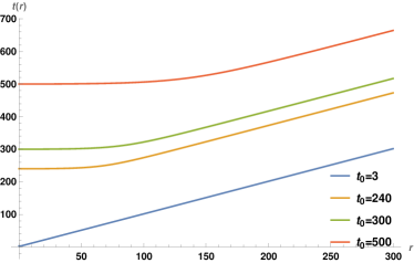
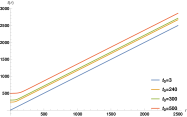
Figure 2: Numerical plots of the complexity surface versus $r$ in AdS₅-Kasner spacetime for different slices of $t_{0}$. In the right Figure, we have extended the range of radial coordinate.

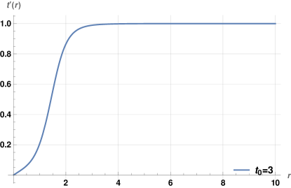
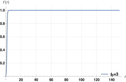
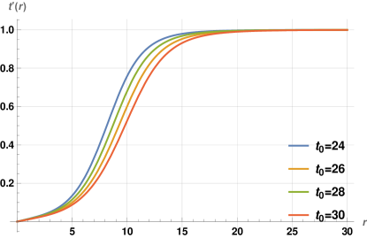
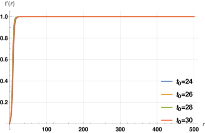
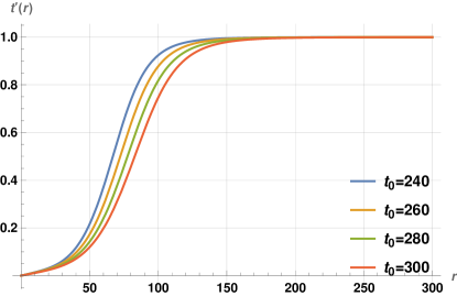
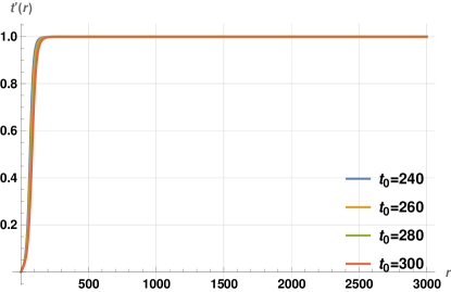
Figure 3: Numerical plots of $t^{\prime}(r)$ versus $r$ in $AdS_{5}$-Kasner spacetime for different $t_{0}$ slices. In the right Figures, we have extended the range of the radial coordinate.

The numerical solutions of (3.3) for the complexity surface $t(r)$ and their derivatives $t^{\prime}(r)$ for different $t_{0}$ slices are plotted in Fig. 2 and Fig. 3 respectively. Some striking points to note are:

• In Fig. 2, we remind the reader that $t(r)$ corresponds to $|t(r)|$ so the singularity is at $t=0$ (the horizontal axis at the bottom). Thus all complexity surfaces bend away from the neighbourhood of the singularity, which correlates with $t^{\prime}(r)>0$.

• From Fig. 2, the complexity surfaces become lightlike after a certain value of $r$ for any anchoring time slice $t_{0}$.

• The surfaces with lower $t_{0}$ (i.e. closer to the singularity) become lightlike earlier (at smaller $r$) than those with larger $t_{0}$. This is also vindicated in Fig. 3, where we have numerically plotted $t^{\prime}(r)$ with $r$. All the complexity surfaces $t(r)$ approach $t^{\prime}(r)=1$ eventually, i.e. a lightlike regime.

• The lightlike regime $t^{\prime}(r)=1$ implies vanishing holographic complexity here from the $\sqrt{1-t^{\prime}(r)^{2}}$ factor in (3.8). Thus, numerically we see that complexity picks up finite contributions only from the near-boundary spacelike part of the complexity surfaces, beyond which it has negligible value where the complexity surfaces are lightlike.

• The above two points imply that as the anchoring time slice approaches the singularity location $t_{0}\rightarrow 0$, the complexity surface is almost entirely lightlike: thus as $t_{0}\rightarrow 0$ the holographic volume complexity becomes vanishingly small. We verify this later by numerical evaluation of the volume complexity integral in sec. 3.4.

• These numerical plots and this analysis only makes sense for $t_{0}$ not strictly vanishing (e.g. we require $t_{0}\gtrsim\epsilon$). In close proximity to the singularity, the semiclassical gravity framework here and our analysis breaks down.

In Figs. 2 and 3, we have shown the behaviour of $t(r)$ and $t^{\prime}(r)$ with $r$ for both limited range (left side plots) and extended range of the radial coordinate in these Figures (right side plots). We obtain similar behavior for other cases later. So we will not show the counterparts of the right side plots (extended $r$-range) in Figs. 2-3 in order to display our results succinctly in subsequent data.

3.2 Holographic complexity of $AdS_{4}$-Kasner spacetime

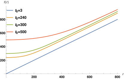
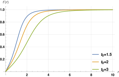
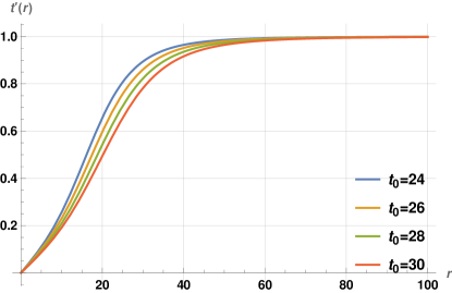
Figure 4: Plots of $t(r)$ with $r$ and $t^{\prime}(r)$ with $r$ in $AdS_{4}$-Kasner spacetime for various $t_{0}$ slices.

For the $AdS_{4}$-Kasner spacetime with $d_{i}=2$, the equation of motion (3.2) for the complexity surface $t(r)$ becomes

$$r\,t(r)\,t^{\prime\prime}(r)-3t(r)\,t^{\prime}(r)\left(1-t^{\prime}(r)^{2}\right)+r\left(1-t^{\prime}(r)^{2}\right)=0\,.$$ (3.17)

Numerical results: The perturbative solution of (3.17) is obtained only up to $O(r^{2})$ unfortunately, i.e. $t(r)=t_{0}+\frac{r^{2}}{4t_{0}}$ , beyond which the numerics appear problematic. However, we find that this $O(r^{2})$ perturbative solution is adequate in extracting the initial conditions for numerical solutions.

Using these initial conditions, the numerical solution of (3.17) for $t(r)$ and its derivative $t^{\prime}(r)$ are obtained along the same lines as in $AdS_{5}$-Kasner. These are plotted in Fig. 4, which reveal that the behaviour of the complexity surfaces $t(r)$ and their derivatives are similar to those in $AdS_{5}$-Kasner.

3.3 Holographic complexity of AdS₇-Kasner spacetime

The equation of motion for the complexity surface $t(r)$ for $AdS_{7}$-Kasner spacetime using $d_{i}=5$ in (3.2) becomes

$$r\,t(r)\,t^{\prime\prime}(r)-6t(r)\,t^{\prime}(r)\left(1-t^{\prime}(r)^{2}\right)+r\left(1-t^{\prime}(r)^{2}\right)=0\,.$$ (3.18)

As in $AdS_{5}$-Kasner spacetime, we solve this perturbatively and numerically.

Perturbative results: The perturbative solution of (3.18) for the ansatz $t(r)=t_{0}+{\bf\sum_{n\in\mathbb{Z}_{+}}}c_{n}r^{n}$ is given as:

$$\hskip-21.68121ptt(r)=t_{0}+\frac{r^{2}}{10t_{0}}-\frac{23r^{4}}{3000t_{0}^{3}}+\frac{889r^{6}}{450000t_{0}^{5}}+\frac{51r^{8}}{2000000t_{0}^{7}}+\frac{13717r^{10}}{1500000000t_{0}^{9}}-\frac{432601r^{12}}{162000000000t_{0}^{11}}-\frac{224725657r^{14}}{1417500000000000t_{0}^{13}}$$

$$\hskip-21.68121pt+\frac{63000761753r^{16}}{5103000000000000000t_{0}^{15}}-\frac{4205482267127r^{18}}{459270000000000000000t_{0}^{17}}+\frac{72021793622269r^{20}}{32805000000000000000000t_{0}^{19}}-\frac{605389181603981r^{22}}{1202850000000000000000000t_{0}^{21}}$$

$$\hskip-21.68121pt+\frac{21913289449767169639r^{24}}{154590282000000000000000000000t_{0}^{23}}-\frac{387788648864019516255533r^{26}}{15909916522500000000000000000000000t_{0}^{25}}$$

$$\hskip-21.68121pt+\frac{5075669610394250085896593r^{28}}{954594991350000000000000000000000000t_{0}^{27}}-\frac{376370639143190660245447709477r^{30}}{345802035616537500000000000000000000000000t_{0}^{29}}.$$ (3.19)

The solution (3.3) for $t(r)$ and its derivative $t^{\prime}(r)$ for $AdS_{7}$-Kasner are qualitatively similar to those in $AdS_{5}$-Kasner.

Numerical results: Using the above, we can pin down boundary conditions near the boundary and then solve (3.18) numerically. This is similar to the analysis in $AdS_{5}$-Kasner and the solution $t(r)$ of (3.18) and its derivative $t^{\prime}(r)$ are plotted in Fig. 5. We see that the $AdS_{7}$-Kasner spacetime gives similar results.

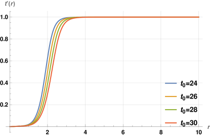
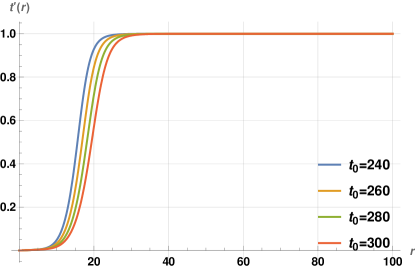
Figure 5: Plots of $t(r)$ with $r$ and $t^{\prime}(r)$ with $r$ in $AdS_{7}$-Kasner spacetime for different $t_{0}$ slices.

3.4 Numerical computation of complexity, $AdS$-Kasner

We evaluate holographic complexity of $AdS_{5,4,7}$-Kasner spacetime numerically using the numerical solutions discussed above and performing the numerical integration in $C$. The expression of holographic complexity for $AdS_{5}$, $AdS_{4}$ and $AdS_{7}$-Kasner spacetimes are given as:

$$({\rm AdS_{d_{i}+2}\ Kasner})\ \ \ \ \ \ \ \ C=\frac{V_{d_{i}}{R^{d_{i}}}}{G_{d_{i}+2}}\int_{\epsilon}dr\,\left({t(r)\ \sqrt{1-t^{\prime}(r)^{2}\,}\over r^{d_{i}+1}}\right)\,.\qquad$$ (3.20)

To perform the integrals numerically, we set the lengthscales $V_{d_{i}},\ R^{d_{i}},\ G_{d_{i}+2}$ to unity and take $\epsilon=10^{-2}$ at the lower end. The upper end of the integration domain is irrelevant since the complexity surfaces become lightlike eventually as $r$ increases so the complexity integral has negligible contribution there, as stated in sec. 3.1.1. Then as an order-of-magnitude estimate, $t_{0}\sim 100$ gives $C\sim{t_{0}\over\epsilon^{d_{i}}}\sim 10^{2d_{i}+2}$ which corroborates with the scales in Fig. 6 which displays the variation

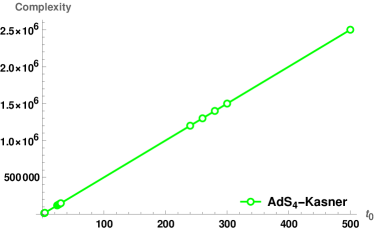
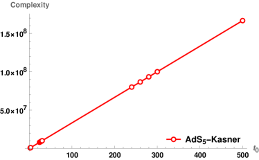
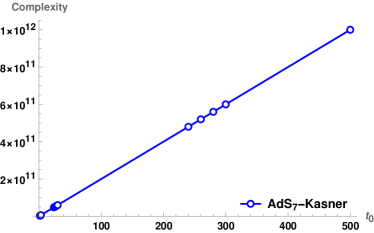
Figure 6: Numerical plots of holographic volume complexity with $t_{0}$ in $AdS_{4,5,7}$-Kasner spacetimes.

of complexity with $t_{0}$ in $AdS$-Kasner spacetime. From the Figure, we see that holographic volume complexity decreases linearly as the anchoring time slice approaches the vicinity of the singularity, i.e. as $t_{0}\rightarrow 0$. Thus the dual Kasner state appears to be of vanishingly low complexity, independent of the reference state.

It is worth making a few comparisons on holographic complexity across $AdS_{5,7,4}$ Kasner spacetimes, based on the numerical results in Fig. 2, Fig. 3 ($AdS_{5}$-K), Fig. 5 ($AdS_{7}$-K), and Fig. 4 ($AdS_{4}$-K). Relative to $AdS_{5}$-Kasner, we see that the complexity surfaces become lightlike at smaller $r$-values in $AdS_{7}$-Kasner. Thus complexity of $AdS_{7}$-Kasner acquires vanishing contributions at smaller $r$-values relative to $AdS_{5}$-Kasner. Likewise, we see that the $AdS_{5}$-Kasner displays the lightlike regime at smaller $r$-values than $AdS_{4}$-Kasner. Thus complexity surfaces in higher dimensional $AdS$-Kasner acquire lightlike regimes earlier than those in lower dimensional ones. However it is clear that the leading divergence behaviour is larger for higher dimensions, since the extremal codim-1 surface volumes have dominant contributions from the near boundary region. With cutoff $\epsilon\equiv\Lambda_{UV}^{-1}$ we have the scaling

$$C\ \sim\ {R^{d_{i}+1}\over G_{d_{i}+2}\,R}\,{V_{d_{i}}\over\epsilon^{d_{i}}}\,t_{0}\ \equiv\ N_{dof}\,V_{d_{i}}\Lambda_{{}_{UV}}^{d_{i}}\,t_{0}\,,$$ (3.21)

reflecting the fact that complexity scales with the number of degrees of freedom in the dual field theory and with spatial volume in units of the UV cutoff. Some intuition for this can be obtained from the form of the complexity volume functional (3.20) where the $\sqrt{1-(t^{\prime})^{2}}$ factor is amplified by the ${1\over r^{d_{i}}}$-factor. Both the spacelike part ($t^{\prime}\ll 1$) of the complexity surface and the transition to the lightlike part (where $t^{\prime}$ is changing) are amplified by the ${1\over r^{d_{i}}}$-factor to a greater degree at larger $d_{i}$. Thus higher dimensional $AdS$-Kasner hits the lightlike regime and vanishing complexity at smaller $r$-values relative to lower dimensions.

Overall from (3.21) we see that

$${dC\over dt_{0}}\ \sim\ N_{dof}\,V_{d_{i}}\Lambda_{{}_{UV}}^{d_{i}}\,,$$ (3.22)

which arises from just the near-boundary UV part of the complexity surface, with the lightlike part giving vanishing contributions. This is consistent with complexity scaling as the number of microscopic degrees of freedom in (a lattice approximation of) the CFT. In this light, it appears that in the vicinity of the singularity, there is a thinning of the effective number of degrees of freedom. As $t_{0}\rightarrow 0$, space entirely Crunches and there are no effective qubits, and so correspondingly complexity vanishes.

4 Complexity: hyperscaling violating cosmologies

Various cosmological deformations of conformally $AdS$ or hyperscaling violating theories were found in [95] (see App. A). The 2-dim form of these backgrounds can be described in terms of the 2-dim dilaton gravity action (2.4) with dilaton potential, parameters, as well as the $(t,r)$-scaling exponents in (2.5) given below. Also appearing below is the higher dimensional cosmology:

$$U=2\Lambda\phi^{1/d_{i}}\,e^{\gamma\Psi}\,,\qquad 2\Lambda=-(d_{i}+1-\theta)(d_{i}-\theta)\,,\qquad\gamma=\frac{-2\theta}{\sqrt{2d_{i}(d_{i}-\theta)(-\theta)}}\,,$$

$$\quad ds^{2}=\frac{{R^{2}}r^{\frac{2\theta}{d_{i}}}}{r^{2}}\Biggl{(}\frac{-dt^{2}+dr^{2}}{t^{\gamma\alpha}}+t^{2/d_{i}}dx_{i}^{2}\Biggr{)},\quad e^{\Psi}=t^{\alpha}r^{\sqrt{2(d_{i}-\theta)\frac{(-\theta)}{d_{i}}}}\,,$$

$$k=1\,,\quad m=-(d_{i}-\theta)\,,\quad a={\alpha^{2}\over 2}\,,\quad\alpha=-\gamma\pm\sqrt{\gamma^{2}+\frac{2(d_{i}-1)}{d_{i}}}\,,$$

$$b=-{(d_{i}-\theta)(d_{i}+1)\over d_{i}}\,,\quad\beta=\sqrt{{2(d_{i}-\theta)(-\theta)\over d_{i}}}\,.$$ (4.1)

With $\alpha$ taken positive, $e^{\Psi}\rightarrow 0$ as $t\rightarrow 0$ and we obtain

$$\alpha=-\gamma+\sqrt{\gamma^{2}+\frac{2(d_{i}-1)}{d_{i}}}\quad\rightarrow\quad a=\left(\sqrt{\frac{d_{i}-\theta-1}{d_{i}-\theta}}-\sqrt{\frac{(-\theta)}{d_{i}(d_{i}-\theta)}}\right)^{2}.$$ (4.2)

In this section, we restrict to Lorentz invariance: the Lifshitz exponent is $z=1$. Then the null energy conditions [100] implies that the hyperscaling violating exponent $\theta$ is constrained as

$$(d_{i}-\theta)(d_{i}(z-1)-\theta)\geq 0\,,\qquad(z-1)(d_{i}+z-\theta)\geq 0\quad\xrightarrow{z=1}\quad\theta\leq 0\,.$$ (4.3)

The other possibility $\theta>d_{i}$ has undesirable properties suggesting instabilities [100].

Time-independent backgrounds of this sort appear in the dimensional reduction [100] over the transverse spheres of nonconformal $Dp$-branes [101], and the $\theta$-exponent is then related to the nontrivial running of the gauge coupling. Reductions of nonconformal $Dp$-branes over the transverse spheres and over the brane spatial dimensions leads to 2-dim dilaton gravity theories [96] with dilaton potentials as in (4) above, and the 2-dim dilaton then leads to a holographic $c$-function encoding the nontrivial renormalization group flows. Some of the analysis there, as well as in [100], may be helpful to keep in mind in our discussions here. In particular, the D2-brane and D4-brane supergravity phases give rise to $d_{i}=2,\ \theta=-{1\over 3}$ and $d_{i}=4,\ \theta=-1$, respectively, both with $z=1$. In these cases, the Big-Bang/Crunch singularities may be interpreted as appropriate Kasner-like deformations of the nonconformal $Dp$-brane backgrounds, although again the time-dependence does not switch off asymptotically with corresponding difficulties in interpretation as severe time-dependent deformations of some vacuum state.

We will focus on these in studying the Big-Bang/Crunch hyperscaling violating cosmological backgrounds in (4) above and study holographic complexity thereof. The calculations are broadly similar to those in $AdS$ Kasner spacetimes earlier, but with interesting detailed differences.

Using the exponents in (4), (4.2), the holographic volume complexity (2.9) simplifies to

$$C=\frac{V_{d_{i}}{R^{d_{i}}}}{G_{d_{i}+2}}\int_{\epsilon}dr\left(r^{\frac{(d_{i}+1)(\theta-d_{i})}{d_{i}}}t(r)^{\frac{1}{2}\left(\left(\sqrt{\frac{d_{i}-\theta-1}{d_{i}-\theta}}-\sqrt{\frac{(-\theta)}{d_{i}(d_{i}-\theta)}}\right)^{2}+\frac{1}{d_{i}}+1\right)}\ \sqrt{1-t^{\prime}(r)^{2}}\right).$$ (4.4)

Extremizing with $t(r)$, we obtain the Euler-Lagrange equation of motion for the complexity surface $t(r)$ as

$$r\left(d_{i}\left(\sqrt{\frac{d_{i}-\theta-1}{d_{i}-\theta}}-\sqrt{\frac{(-\theta)}{d_{i}(d_{i}-\theta)}}\right)^{2}+d_{i}+1\right)\left(1-t^{\prime}(r)^{2}\right)$$

$$\qquad\quad+\ 2d_{i}\,r\,t(r)\,t^{\prime\prime}(r)-2(d_{i}+1)(d_{i}-\theta)\,t(r)\,t^{\prime}(r)\left(1-t^{\prime}(r)^{2}\right)=0\,.$$ (4.5)

In the semiclassical limit ($t^{\prime}(r)\ll 1$), we can ignore terms like $t^{\prime}(r)^{2},t^{\prime}(r)^{3}$ in the equation of motion (4), which then simplifies to

$$\hskip-28.90755ptt(r)\left(2(d_{i}+1)(d_{i}-\theta)t^{\prime}(r)-2d_{i}rt^{\prime\prime}(r)\right)-r\left(d_{i}\left(\sqrt{\frac{d_{i}-\theta-1}{d_{i}-\theta}}-\sqrt{\frac{(-\theta)}{d_{i}(d_{i}-\theta)}}\right)^{2}+d_{i}+1\right)=0.$$

Now, we solve equations (4) and (4) perturbatively using ansatze similar to those in the $AdS$-Kasner spacetime, i.e. $t(r)=t_{0}+\sum_{n\in\mathbb{Z}_{+}}c_{n}r^{n}$ . We illustrate this in detail by analysing holographic volume complexity for two cases: (i) $d_{i}=2,\ \theta=-1/3$ in sec. 4.1, and (ii) $d_{i}=4,\ \theta=-1$ in sec. 4.2. Analysing other cases reveals similar results. To differentiate between the different solutions, we will use different coefficients for the different cases, e.g., $g_{n}$, $s_{n}$ etc.

4.1 $d_{i}=2,\ \theta=-{1\over 3}$

This case is related to the $D2$-brane supergravity phase as stated earlier, and we analyze the perturbative and numerical solutions now.

The equation of motion (4) with exponents (4), (4.2), for this case simplifies to

$$14r\,t(r)\,t^{\prime\prime}(r)-\left(2\sqrt{2}-15\right)r\left(1-t^{\prime}(r)^{2}\right)-49t(r)\,t^{\prime}(r)\left(1-t^{\prime}(r)^{2}\right)=0\,.$$ (4.7)

The solution $t(r)$ up to ${\cal O}(r^{30})$ is given as

$$t(r)=t_{0}+g_{2}r^{2}+g_{4}r^{4}+.....+g_{28}r^{28}+g_{30}r^{30}\,,$$ (4.8)

with $g_{i}$ in (• ‣ B). The behaviour of the complexity surfaces (4.8) with $r$ for different $t_{0}$ values is qualitatively similar to those in $AdS$-Kasner (see Fig. 1) so we will not display the plots.

When $t^{\prime}(r)\ll 1$, we can ignore the higher order terms in (4.7) to obtain

$$2\left(2\sqrt{2}-15\right)r-14t(r)\left(2rt^{\prime\prime}(r)-7t^{\prime}(r)\right)=0.$$ (4.9)

This has solution up to ${\cal O}(r^{30})$ given as

$$t(r)=t_{0}+s_{2}r^{2}+s_{4}r^{4}+.....+s_{28}r^{28}+s_{30}r^{30}\,,$$ (4.10)

with $s_{i}$ in (• ‣ B). The behaviour of (4.10) is qualitatively similar to that in $AdS$-Kasner.

Solving (4.7) numerically along similar lines as in $AdS$-Kasner, we obtain the variation of the complexity surfaces and their derivatives with $r$: this is shown in Fig. 7.

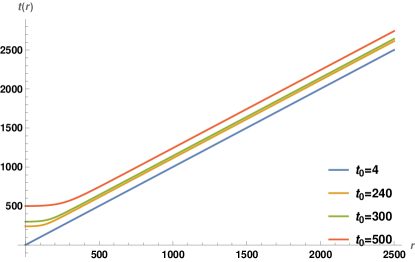
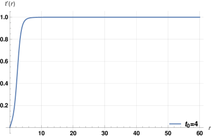
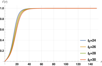
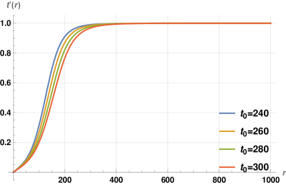
Figure 7: Numerical plots of $t(r)$ versus $r$ and $t^{\prime}(r)$ versus $r$ for $d_{i}=2$ and $\theta=-1/3$ in hv cosmology.

Holographic complexity: With $d_{i}=2,\ \theta=-{1\over 3}$ in (4.4) gives

$$C=\frac{V_{2}{R^{2}}}{G_{4}}\int_{\epsilon}dr\left(\frac{t(r)^{\frac{15}{14}-\frac{\sqrt{2}}{7}}\sqrt{1-t^{\prime}(r)^{2}}}{r^{7/2}}\right).$$ (4.11)

Restricting to the regime $t^{\prime}(r)\ll 1$, we perform this integral rewriting as

$$C=\frac{V_{2}{R^{2}}}{G_{4}}\int_{\epsilon}^{r_{\Lambda}}dr\left(\frac{t(r)^{\frac{15}{14}-\frac{\sqrt{2}}{7}}\left({1-\frac{t^{\prime}(r)^{2}}{2}}\right)}{r^{7/2}}\right).$$ (4.12)

Then using (4.10) truncating to $t(r)=t_{0}+s_{2}r^{2}+s_{4}r^{4}$ using (• ‣ B), the complexity (4.12) up to next-to-leading-order in $t_{0}$ is obtained as

$$C=\frac{V_{2}{R^{2}}}{G_{4}}\left(\frac{2}{5}t_{0}^{\frac{15}{14}-\frac{\sqrt{2}}{7}}\left(\frac{1}{\epsilon^{5/2}}-\frac{1}{r_{\Lambda}^{5/2}}\right)-\frac{2883\left(\frac{1}{t_{0}}\right)^{\frac{13}{14}+\frac{\sqrt{2}}{7}}\left(\frac{1}{\sqrt{r_{\Lambda}}}-\frac{1}{\sqrt{\epsilon}}\right)}{50\left(233+60\sqrt{2}\right)}\right).$$ (4.13)

4.2 $d_{i}=4,\ \theta=-1$

This is related to the $D4$-brane supergravity phase as stated earlier.

For $d_{i}=4$ and $\theta=-1$, the equation of motion (4) becomes

$$20\,r\,t(r)\,t^{\prime\prime}(r)+17\,r\left(1-t^{\prime}(r)^{2}\right)-125\,t(r)\,t^{\prime}(r)\left(1-t^{\prime}(r)^{2}\right)=0\,.$$ (4.14)

Using the ansatz $t(r)=t_{0}+\sum_{n\in\mathbb{Z}_{+}}y_{n}r^{n}$, we obtain the following solution to (4.14):

$$t(r)=t_{0}+y_{2}r^{2}+y_{4}r^{4}+.....+y_{28}r^{28}+y_{30}r^{30}\,,$$ (4.15)

with $y_{i}$ given in (• ‣ B). The plots of the solution (4.15) and its derivatives are qualitatively similar to those in $AdS$-Kasner spacetimes and the $d_{i}=2,\theta=-{1\over 3}$ hv-cosmology. Ignoring higher order terms in (4.14), we obtain

$$-34r+5t(r)\left(-8rt^{\prime\prime}(r)+50t^{\prime}(r)\right)=0\,.$$ (4.16)

Solving this with the ansatz $t(r)=t_{0}+\sum_{n\in\mathbb{Z}_{+}}v_{n}r^{n}$ gives the qualitatively similar complexity surface (with $v_{i}$ in (• ‣ B)):

$$t(r)=t_{0}+v_{2}r^{2}+v_{4}r^{4}+.....+v_{28}r^{28}+v_{30}r^{30}\,.$$ (4.17)

Solving the nonlinear equation (4.14) numerically as in $AdS$-Kasner gives numerical solutions for the complexity surfaces $t(r)$ and their derivatives. These are shown in Fig. 8.

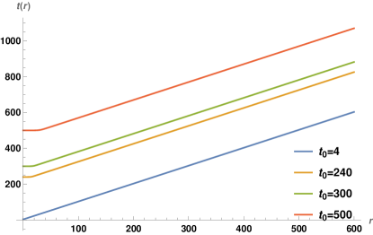
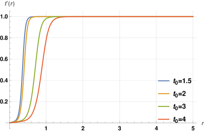
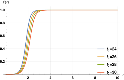
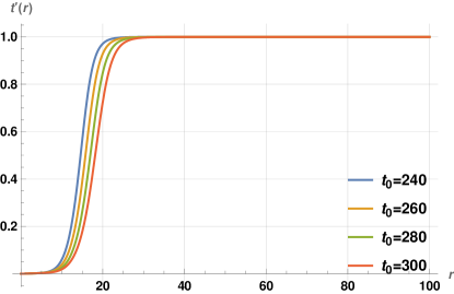
Figure 8: Plots of complexity surface versus $r$ and $t^{\prime}(r)$ versus $r$ for $d_{i}=4$ and $\theta=-1$ in hyperscaling violating cosmology.

Holographic complexity: Substituting $d_{i}=4,\ \theta=-1$ in (4.4) gives

$$C=\frac{V_{4}{R^{4}}}{G_{6}}\int_{\epsilon}dr\left(\frac{t(r)^{17/20}\sqrt{1-t^{\prime}(r)^{2}}}{r^{25/4}}\right)\ \sim\ \frac{V_{4}{R^{4}}}{G_{6}}\int_{\epsilon}^{r_{\Lambda}}dr\left(\frac{t(r)^{17/20}\left(1-\frac{t^{\prime}(r)^{2}}{2}\right)}{r^{25/4}}\right).$$ (4.18)

Similar to the discussion for $d_{i}=2,\theta=-{1\over 3}$, we approximate as $t(r)=t_{0}+v_{2}r^{2}+v_{4}r^{4}$ (with $v_{2}$, $v_{4}$ in (• ‣ B)) and simplify (4.18). The calculations are similar to the earlier case: complexity up to next-to-leading-order in $t_{0}$ is

$$\hskip-36.135ptC=\frac{V_{4}{R^{4}}}{G_{6}}\Biggl{[}t_{0}^{17/20}\left(\frac{4}{21\epsilon^{21/4}}-\frac{4}{21{r_{\Lambda}}^{21/4}}\right)$$

$$\hskip-21.68121pt+\left(\frac{1}{t_{0}}\right)^{23/20}\left(\frac{4913}{525\left(\sqrt{715}-13\right)\left(13+\sqrt{715}\right)\epsilon^{13/4}}-\frac{4913}{525\left(\sqrt{715}-13\right)\left(13+\sqrt{715}\right){r_{\Lambda}}^{13/4}}\right)\Biggr{]}.$$

{$d_{i}=2,\ \theta=-{1\over 3}$} vs {$d_{i}=4,\ \theta=-1$} hv-cosmologies:  Comparing Fig. 7 and Fig. 8, we see that the numerical solution of $d_{i}=4,\ \theta=-1$ hv-cosmology becomes lightlike for a smaller $r$-value relative to that for $d_{i}=2,\ \theta=-{1\over 3}$ . The $\sqrt{1-t^{\prime}(r)^{2}}$ factor in the volume complexity expression implies $d_{i}=4,\ \theta=-1$ complexity vanishing earlier relative to that in $d_{i}=2,\ \theta=-{1\over 3}$ . These theories have effective space dimension $d_{eff}=d_{i}-\theta$ so the effective dimensions are $d_{eff}=5$ and $d_{eff}={7\over 3}$ respectively: so the larger effective dimension case acquires vanishing complexity at smaller $r$-values. This is similar to the observations in $AdS$-Kasner discussed in sec. 3.4.

Let us summarize the results for complexity in $AdS_{5}$-Kasner and hyperscaling violating cosmologies up to next-to-leading-order in $t_{0}$ (the results to this order are the same whether we use the linearized equation ignoring higher order terms in $t^{\prime}(r)$, or the full nonlinear one):

$$\hskip-21.68121pt({\rm AdS_{5}-Kasner})\ \ \ \ \ \ \ \ C\approx\frac{V_{3}{R^{3}}}{G_{5}}\Biggl{[}t_{0}\left(\frac{0.3}{\epsilon^{3}}-\frac{0.3}{r_{\Lambda}^{3}}\right)+\frac{1}{t_{0}}\left(\frac{0.1}{\epsilon}-\frac{0.1}{r_{\Lambda}}\right)+O\left(\left(\frac{1}{t_{0}}\right)^{3}\right)\Biggr{]},$$

$$\hskip-21.68121pt\left(d_{i}=2,\ \theta=-{1\over 3}\right)\ \ \ \ C\approx\frac{V_{2}{R^{2}}}{G_{4}}\left(\frac{2}{5}t_{0}^{\frac{15}{14}-\frac{\sqrt{2}}{7}}\left(\frac{1}{\epsilon^{5/2}}-\frac{1}{r_{\Lambda}^{5/2}}\right)-\frac{2883\left(\frac{1}{t_{0}}\right)^{\frac{13}{14}+\frac{\sqrt{2}}{7}}\left(\frac{1}{\sqrt{r_{\Lambda}}}-\frac{1}{\sqrt{\epsilon}}\right)}{50\left(233+60\sqrt{2}\right)}\right),$$

$$\hskip-21.68121pt(d_{i}=4,\ \theta=-1)\ \ \ \ \ \ \ C\approx\frac{V_{4}{R^{4}}}{G_{6}}\Biggl{[}t_{0}^{17/20}\left(\frac{4}{21\epsilon^{21/4}}-\frac{4}{21{r_{\Lambda}}^{21/4}}\right)$$

$$\hskip-21.68121pt+\left(\frac{1}{t_{0}}\right)^{23/20}\left(\frac{4913}{525\left(\sqrt{715}-13\right)\left(13+\sqrt{715}\right)\epsilon^{13/4}}-\frac{4913}{525\left(\sqrt{715}-13\right)\left(13+\sqrt{715}\right){r_{\Lambda}}^{13/4}}\right)\Biggr{]}.$$

The leading divergence of complexity from above is $C=\frac{V_{2}{R^{2}}}{G_{4}\epsilon^{5/2}}\,t_{0}^{\frac{15-2\sqrt{2}}{14}}$ for $d_{i}=2,\theta=-{1\over 3}$, and $C=\frac{V_{4}{R^{4}}}{G_{6}\epsilon^{21/4}}\,t_{0}^{17/20}$ for $d_{i}=4,\theta=-1$. Overall, at leading order in (4.2), we see that the holographic complexity of AdS₅-Kasner spacetime is linearly proportional to $t_{0}$ whereas in hyperscaling violating cosmologies, complexity is proportional to $t_{0}^{0.9}$ and $t_{0}^{0.85}$ summarized below:

$$\qquad\qquad\qquad\qquad({\rm AdS_{5}-Kasner})\ \ \ \ \ \ \ \ \ \ \ C\propto t_{0}\,,$$

$$\left(d_{i}=2,\ \theta=-{1\over 3}\right)\ \ \ \ \ \ \ \ C\propto t_{0}^{0.9}\,,\qquad\qquad(d_{i}=4,\ \theta=-1)\ \ \ \ \ \ \ \ \ \ \ C\propto t_{0}^{0.85}\,.\qquad$$ (4.21)

The complexity scaling in hv-cosmologies reflects the fact that the dual theories live in some sort of effective space dimension $d_{eff}=d_{i}-\theta$. It might be interesting to understand the underlying effective lattice qubit models simulating this behaviour (these are perhaps distinct from relativistic CFTs, in light of the general arguments in [3]).

4.3 Numerical computation of complexity in hv cosmologies

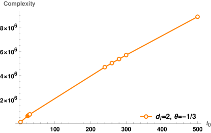
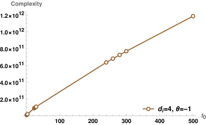
Figure 9: Numerical plots of holographic complexity versus $t_{0}$ for $d_{i}=2,\ \theta=-1/3$ and $d_{i}=4,\ \theta=-1$ cosmologies.

We now compute holographic complexity of hyperscaling violating cosmologies, for $d_{i}=2,\ \theta=-{1\over 3}$, and $d_{i}=4,\ \theta=-1$, as for $AdS$-Kasner spacetimes in sec. 3.4. For this purpose, we use the numerical solutions of the cosmologies as discussed earlier, and numerically perform the integrations appearing in the complexity expressions in (4.11) for $d_{i}=2,\ \theta=-{1\over 3}$, and (4.18) for $d_{i}=4,\ \theta=-1$ (using the full nonlinear expression). The variation of holographic complexity with $t_{0}$ in these backgrounds is shown in Fig. 9.

As we see in (4.2), the complexity of hyperscaling violating cosmologies does not scale linearly with $t_{0}$, unlike that in $AdS$-Kasner spacetimes. However the exponents are positive so complexity continues to decrease with $t_{0}$ moving towards the singularity, becoming vanishingly small as $t_{0}\rightarrow 0$. Thus the dual Kasner state continues to exhibit low complexity, as displayed in Fig. 9.

5 Complexity: isotropic Lifshitz Kasner cosmologies

The 2-dim dilaton gravity formulation [95] led to new Kasner cosmologies with Lifshitz asymptotics. The equations of motion are rather constraining however admitting only certain values for the various exponents: in particular the cosmological solutions turn out to have $\theta=0$ so $\gamma=0$ with Lifshitz exponent $z=d_{i}$. In 2-dim form, they are described by the 2-dim dilaton gravity action (2.4) with dilaton potential, parameters, and the $(t,r)$-scaling exponents in (2.5) below. Also given below is the higher dimensional Lifshitz Kasner cosmology:

$$U=\phi^{1/d_{i}}\Big{(}-c_{1}+{c_{2}\over\phi^{2}}e^{\lambda\Psi}\Big{)}\,,\quad\lambda=-\sqrt{{2d_{i}\over d_{i}-1}}\,,\quad c_{1}={2(2d_{i}-1)\over d_{i}}\,\quad c_{2}={2(d_{i}-1)\over d_{i}}\,,$$

$$\qquad\qquad ds^{2}=R^{2}\left(-{dt^{2}\over r^{2z}}+{dr^{2}\over r^{2}}+t^{2/d_{i}}{dx_{i}^{2}\over r^{2}}\right),\qquad e^{\Psi}=t^{\alpha}r^{-\alpha}\,,\quad z=d_{i}\,,$$ (5.1)

$$k=1,\quad m=-1\,,\quad a={d_{i}-1\over d_{i}}\,,\quad b=-3+{1\over d_{i}}\,,\quad-\beta=\alpha=-\sqrt{{2(d_{i}-1)\over d_{i}}}\,.\ \$$

Here $R$ is the analog of the $AdS$ scale, and we are suppressing an additional scale in $g_{tt}$ arising due to the nontrivial Lifshitz scaling. The nonrelativistic time-space scaling implies that lightlike trajectories have $dt^{2}=r^{2z-2}dr^{2}$ so to identify lightlike limits it is convenient to use $(t,\rho)$ coordinates with $\rho\sim r^{z}$. To illustrate this and study complexity, we will focus on the Lifshitz Kasner cosmology with $z=d_{i}=2$ and exponents $a={1\over 2}$ , $b=-{5\over 2}$  with metric

$$ds^{2}={R^{2}}\left(-\frac{dt^{2}}{r^{4}}+\frac{dr^{2}}{r^{2}}+\frac{t}{r^{2}}\left(dx_{1}^{2}+dx_{2}^{2}\right)\right).$$ (5.2)

Redefining $r^{2}\sim\rho$ and appropriately absorbing numerical factors redefining the various lengthscales makes lightlike trajectories have $dt^{2}=d\rho^{2}$, with the metric (5.2) recast as

$$ds^{2}={R^{2}}\left(-\frac{dt^{2}}{\rho^{2}}+\frac{d\rho^{2}}{\rho^{2}}+\frac{t}{\rho}(dx_{1}^{2}+dx_{2}^{2})\right).$$ (5.3)

Parametrizing the complexity surface by $t(\rho)$ gives the complexity volume functional

$$C=\frac{V_{2}{R^{3}}}{G_{4}R}\int_{\epsilon}d\rho\left(\frac{t(\rho)}{\rho^{2}}\sqrt{1-(t^{\prime}(\rho))^{2}}\right),$$ (5.4)

with $V_{2}=\int dx_{1}dx_{2}$. Extremizing for the complexity surface $t(\rho)$ gives the equation of motion

$$\rho\,t(\rho)\,t^{\prime\prime}(\rho)-2t(\rho)\,t^{\prime}(\rho)(\left(1-t^{\prime}(\rho)^{2}\right)+\rho\left(1-t^{\prime}(\rho)^{2}\right)=0\,.$$ (5.5)

The perturbative solution of (5.5) for the ansatz $t(\rho)=\sum_{n\in\mathbb{Z}_{+}}c_{n}\rho^{n}$ similar to the previous cases up to ${\cal O}(\rho^{30})$ is given by

$$\hskip-14.45377ptt(\rho)={t_{0}}+\frac{\rho^{2}}{2{t_{0}}}-\frac{\rho^{4}}{8{t_{0}}^{3}}+\frac{\rho^{6}}{16{t_{0}}^{5}}-\frac{5\rho^{8}}{128{t_{0}}^{7}}+\frac{7\rho^{10}}{256{t_{0}}^{9}}-\frac{21\rho^{12}}{1024{t_{0}}^{11}}+\frac{33\rho^{14}}{2048{t_{0}}^{13}}-\frac{429\rho^{16}}{32768{t_{0}}^{15}}+\frac{715\rho^{18}}{65536{t_{0}}^{17}}$$ (5.6)

$$\qquad-\frac{2431\rho^{20}}{262144{t_{0}}^{19}}+\frac{4199\rho^{22}}{524288{t_{0}}^{21}}-\frac{29393\rho^{24}}{4194304{t_{0}}^{23}}+\frac{52003\rho^{26}}{8388608{t_{0}}^{25}}-\frac{185725\rho^{28}}{33554432{t_{0}}^{27}}+\frac{334305\rho^{30}}{67108864{t_{0}}^{29}}\,.\ \ \$$

The behavior of this perturbative solution is qualitatively similar to that in $AdS$-Kasner and hv-cosmologies, so we suppress these plots here.

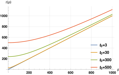
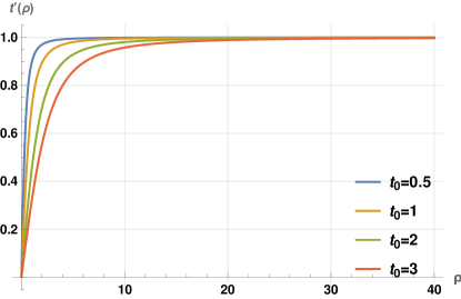
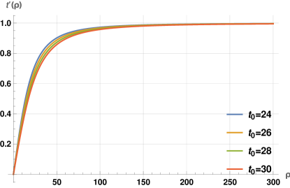
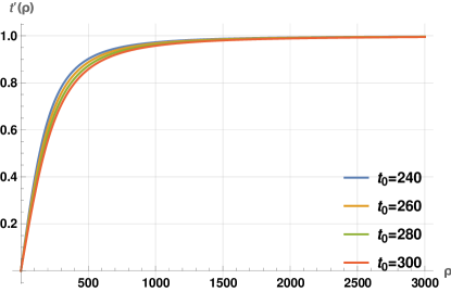
Figure 10: Variation of volume complexity surfaces $t(\rho)$ and their derivative $t^{\prime}(\rho)$ with radial distance $\rho$ for 4-dim Lifshitz Kasner cosmology.

As in the earlier cases, it is instructive to study the complexity surface equation numerically, so we solve (5.5) with boundary conditions for $t(\rho)$ and $t^{\prime}(\rho)$ at the boundary $\rho=\epsilon_{\rho}$ with appropriate numerical values for $\epsilon_{\rho}$, along similar lines as described earlier. The numerical results are shown in Fig. 10 which display the variation of the complexity surfaces and their derivatives with $\rho$ for various $t_{0}$ values. The plots show that the transition to the lightlike regime is slower with nontrivial Lifshitz $z$-exponent (relative to $AdS$, $z=1$).

Perturbatively we can compute holographic complexity in the regime $\rho\lesssim t_{0}$ where $t^{\prime}(\rho)<1$, approximating complexity (5.4) as

$$C\sim\frac{V_{2}R^{2}}{G_{4}}\int_{\epsilon_{\rho}}^{\rho_{\Lambda}}d\rho\Biggl{[}\frac{t(\rho)}{\rho^{2}}\left({1-\frac{t^{\prime}(\rho)^{2}}{2}}\right)\Biggr{]}.$$ (5.7)

For the perturbative solution (5.6), holographic complexity after truncating (5.7) up to next-to-leading-order in $t_{0}$ is given by

$$C\approx\frac{V_{2}R^{2}}{G_{4}}\Biggl{[}t_{0}\left(\frac{1}{\epsilon_{\rho}}-\frac{1}{\rho_{\Lambda}}\right)+\frac{\left(\rho_{\Lambda}^{3}-\epsilon_{\rho}^{3}\right)}{24t_{0}^{3}}+{\cal O}\left(\frac{1}{t_{0}}\right)^{5}\Biggr{]}.$$ (5.8)

We have described the $z=2$ Lifshitz Kasner cosmology so far: other $z=d_{i}$ cases in $(d_{i}+2)$-dims exhibit similar behaviour. The ($t,\rho$) coordinates with $\rho\sim r^{z}$ in Lifshitz Kasner cosmologies allow us to conveniently see that the complexity surfaces become lightlike in the bulk. The metric in (5) is recast as

$$ds^{2}={R^{2}}\left(-\frac{dt^{2}}{\rho^{2}}+\frac{d\rho^{2}}{\rho^{2}}+{t^{2/z}\over\rho^{2/d_{i}}}dx_{i}^{2}\right)\quad\rightarrow\quad C={V_{d_{i}}\,R^{d_{i}}\over G_{d_{i}+2}}\int d\rho\,{t(\rho)\over\rho^{2}}\sqrt{1-(t^{\prime}(\rho))^{2}}\,.$$ (5.9)

The leading divergence in $C$ is

$$C\sim\frac{R^{d_{i}}}{G_{d_{i}+2}}\,{V_{d_{i}}\over\epsilon_{r}^{d_{i}}}\,t_{0}\,,\qquad\qquad\epsilon_{\rho}=\epsilon_{r}^{z}=\epsilon_{r}^{d_{i}}\,.$$ (5.10)

The above equation shows the linear time growth of complexity in Lifshitz Kasner. Further, from (5.10), we can show that

$$\frac{dC}{dt_{0}}\ \sim\ N_{dof}\,V_{d_{i}}\Lambda_{{}_{UV}}^{d_{i}}\,,$$ (5.11)

where $\epsilon_{\rho}\sim\epsilon_{r}^{d_{i}}\equiv\Lambda_{{}_{UV}}^{d_{i}}$.

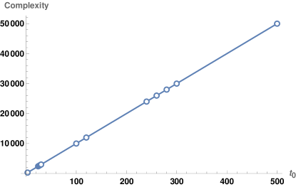
Figure 11: Variation of complexity with $t_{0}$ for 4-dim Lifshitz Kasner cosmology.

The observations in sec. 3.1.1 and sec. 3.4 thus apply here as well upon analysing (5.9), and the dual state appears to have vanishingly low complexity as one approaches the singularity. This is vindicated in Fig. 11 which shows holographic complexity plotted against $t_{0}$ which reveals a linear decrease as the anchoring time slice approaches the singularity, i.e. $t_{0}\rightarrow 0$.

6 Holographic entanglement entropy: $AdS$ Kasner etc

We will review the discussion in [87] here. Classical extremal surfaces in cosmological backgrounds are parametrized by $\left(t(r),x(r)\right)$, $\Delta x=l$, and $t(r)\xrightarrow{r\rightarrow 0}t_{0}$. The time function $t(r)$ exhibits nontrivial bending due to the time-dependence. This extremal surface is located at a constant $t$ slice on the boundary denoted by $t=t_{0}$ and dips into the bulk up to the turning point and returns to $t_{0}$. Here $l$ is the width of the strip along the $x$ direction (taking some $x^{1}=x$), and the extremal surface wraps the other $x_{j\neq 1}$ directions. The holographic entanglement entropy becomes

$$S_{\rm EE}=\frac{1}{4G_{d_{i}+2}}\int\prod_{x_{j}\neq x}^{j=1,2,...,(d_{i}-1)}\left(\phi^{1/d_{i}}dx_{j}\right)\sqrt{\frac{e^{f}}{\phi^{(d_{i}-1)/d_{i}}}(-dt^{2}+dr^{2})+\phi^{2/d_{i}}dx^{2}}\,.$$ (6.1)

The absence of $x(r)$ in (6.1) leads to a conserved conjugate momentum: solving for $x^{\prime}(r)$ gives

$$(x^{\prime}(r))^{2}=A^{2}\,\frac{\frac{e^{f}}{\phi^{(d_{i}+1)/d_{i}}}\left(1-t^{\prime}(r)^{2}\right)}{\phi^{2}-A^{2}}\,.$$ (6.2)

Substituting back into (6.1) gives

$$S_{\rm EE}=\frac{V_{d_{i}-1}}{4G_{d_{i}+2}}\int dr\left(\frac{e^{f/2}\phi^{(3-1/d_{i})/2}}{\sqrt{\phi^{2}-A^{2}}}\right)\sqrt{1-t^{\prime}(r)^{2}}.$$ (6.3)

At the turning point, $x^{\prime}(r)\rightarrow\infty$ implying $A=\phi_{*}=\frac{t_{*}}{r_{*}^{|m|}}$ (in the approximation $\phi$ is nonvanishing and $t^{\prime}(r)\ll 1$) where $t_{*}=t(r_{*})$ (since, $\phi=t^{k}r^{m}$, $k=1$, $m=-|m|<0$).

For the $AdS$ Kasner spacetime, (6.2), (6.3), simplify to

$$x^{\prime}(r)^{2}=A^{2}\left(\frac{1}{t^{2/d_{i}}}\right)\frac{1-t^{\prime}(r)^{2}}{\frac{t^{2}}{r^{2d_{i}}}-A^{2}}\,,\qquad S_{\rm EE}=\frac{V_{d_{i}-1}}{4G_{d_{i}+2}}\int dr\left(\frac{t^{2-1/d_{i}}}{r^{2d_{i}}}\right)\frac{\sqrt{1-t^{\prime}(r)^{2}}}{\sqrt{\frac{t^{2}}{r^{2d_{i}}}-A^{2}}}\,.$$ (6.4)

Using $A=\phi_{*}$, $u=\frac{r}{r_{*}}$, we find the width scaling

$$\frac{l}{2}=\int_{0}^{r_{*}}drx^{\prime}(r)=r_{*}\int_{0}^{1}\frac{du}{t^{1/d_{i}}}\frac{\sqrt{1-t^{\prime}(r)^{2}}}{\sqrt{(\phi/\phi_{*})^{2}-1}}\ \ \Rightarrow\ \ l\sim r_{*}\,,\quad A=\phi_{*}=\frac{t_{*}}{r_{*}^{d_{i}}}\,.$$ (6.5)

For a subregion anchored at a time slice $t_{0}\gg 0$ far from the singularity, the RT/HRT surface bends in time mildly away from the singularity. The turning point is $(t_{*},r_{*})$, with $A>0$ as above for finite size subregions. The IR limit where the subregion becomes the entire space is defined as $l\rightarrow\infty$ and we expect $r_{*}\rightarrow\infty$ so the surface extends deep into the interior: here $A=0$. In the semiclassical region far from the singularity $t_{0}\rightarrow\infty$, solving the extremization equation perturbatively for $t(r)=t_{0}+\sum_{n\in\mathbb{Z}_{+}}c_{n}r^{n}$ shows that $t_{*}\gtrsim t_{0}$ with $t^{\prime}(r)\ll 1$ for finite subregions [87] (reviewed numerically in App. C). This perturbative analysis is similar to that for the complexity surface discussed earlier (see Fig. 1). Analysing this in the IR limit is more tricky. In what follows we will analyse this numerically for the entangling RT/HRT surfaces and find results similar to those for the complexity surfaces.

7 Entanglement, $AdS$-Kasner: numerical results

In this section, we will numerically analyze the codim-2 RT/HRT surfaces for entanglement entropy numerically, building on the studies in [87], along the same lines as complexity. First we obtain the perturbative solution of the equation of motion for $t(r)$ and then use this perturbative solution for boundary conditions to solve numerically. The extremization equation for $t(r)$ following from the entanglement area functional (6.4) is (there is a typo in one of the corresponding equations in [87] but the analysis there is correct)

$$\left(1-t^{\prime}(r)^{2}\right)\left(d_{i}^{2}t^{\prime}(r)+\frac{r\left(t(r)^{2}-A^{2}r^{2d_{i}}\right)}{t(r)^{3}}-\frac{d_{i}r}{t(r)}\right)-\frac{\left(t(r)^{2}-A^{2}r^{2d_{i}}\right)d_{i}rt^{\prime\prime}(r)}{t(r)^{2}}=0\,.$$ (7.1)

We will focus on solving (7.1) in the IR limit $A=0$ (6.5) for infinitely wide strip subregions in $AdS_{5,7}$-Kasner spacetimes in sec. 7.1 and sec. 7.2 respectively. The above equation in the IR limit $A=0$ becomes

$$d_{i}\,r\,t(r)\,t^{\prime\prime}(r)\,-\,\left(1-t^{\prime}(r)^{2}\right)\big{(}d_{i}^{2}\,t(r)\,t^{\prime}(r)-(d_{i}-1)r\big{)}=0\,.$$ (7.2)

7.1 Holographic entanglement entropy in $AdS_{5}$-Kasner

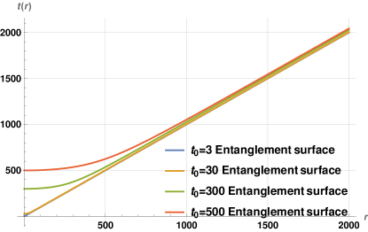
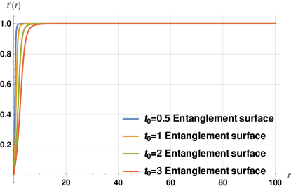
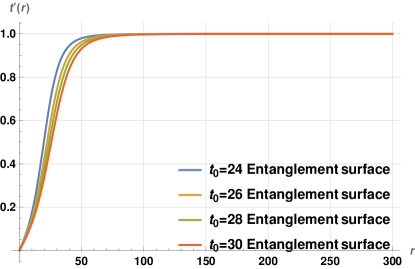
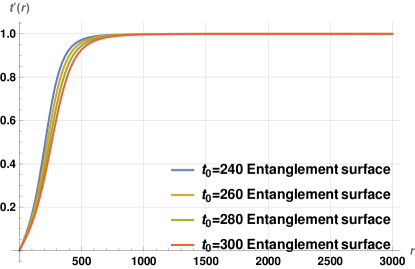
Figure 12: Variations of the RT/HRT surface $t(r)$ vs $r$ and $t^{\prime}(r)$ vs $r$ in $AdS_{5}$-Kasner spacetime for various $t_{0}$ slices.

For $AdS_{5}$-Kasner with $d_{i}=3$, the IR limit (7.2) becomes

$$3\,r\,t(r)\,t^{\prime\prime}(r)\,-\,\left(1-t^{\prime}(r)^{2}\right)\big{(}9\,t(r)\,t^{\prime}(r)-2r\big{)}=0\,.$$ (7.3)

The perturbative solution of (7.3) using the ansatz $t(r)=t_{0}+\sum_{n\in\mathbb{Z}_{+}}c_{n}r^{n}$, after truncating, is

$$t(r)\sim t_{0}+\frac{r^{2}}{6t_{0}}\,.$$ (7.4)

The numerical solutions of (7.3) and their derivatives are shown in Fig. 12. This shows that the behaviour of RT/HRT surfaces is similar to complexity surfaces, as discussed earlier. In particular, the RT/HRT surface for lower $t_{0}$ (closer to the singularity) becomes lightlike earlier in comparison to RT surfaces with higher $t_{0}$ values. Thus as we approach the singularity with $t_{0}\rightarrow 0$, entanglement entropy becomes vanishingly small. In particular near the singularity, entanglement entropy vanishes as did complexity. There is an extreme thinning of the degrees of freedom near the singularity.

For $AdS_{4}$-Kasner, the results are qualitatively similar but the numerics turn out to not be as clean for just technical rather than physics reasons so we do not discuss this.

7.2 Holographic entanglement entropy, $AdS_{7}$-Kasner

The $t(r)$ equation of motion in the IR limit (7.2) for $AdS_{7}$-Kasner spacetime with $d_{i}=5$ is:

$$5\,r\,t(r)\,t^{\prime\prime}(r)\,-\,\left(1-t^{\prime}(r)^{2}\right)\big{(}25\,t(r)\,t^{\prime}(r)-4r\big{)}=0\,.$$ (7.5)

The perturbative solution of (7.5) using the ansatz $t(r)=t_{0}+\sum_{n\in\mathbb{Z}_{+}}c_{n}r^{n}$ is obtained as:

$$t(r)=t_{0}+\frac{r^{2}}{10t_{0}}-\frac{9r^{4}}{1000t_{0}^{3}}.$$ (7.6)

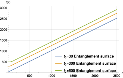
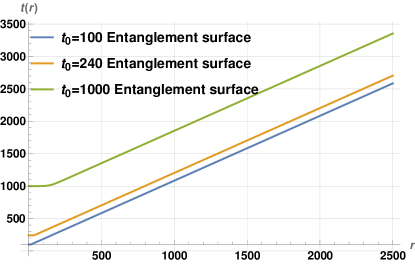
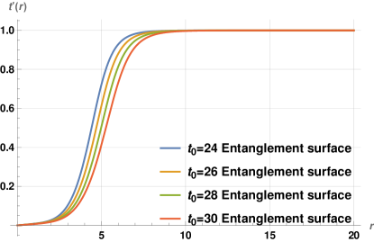
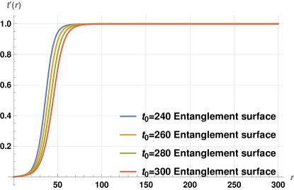
Figure 13: Numerical plots of the RT/HRT surfaces $t(r)$ versus $r$ and $t^{\prime}(r)$ versus $r$ in AdS₇-Kasner spacetime for different $t_{0}$ slices.

The numerical solutions of (7.5) and their derivatives are shown in Fig. 13: we find the entangling surfaces $t(r)$ have qualitatively similar behaviour as in $AdS_{5}$-Kasner.

7.3 Numerical computation of holographic entanglement entropy

The holographic entanglement entropy (6.4) in the IR limit $A=0$ for $AdS_{d_{i}+2}$-Kasner spacetime becomes

$$S_{\rm EE}=\frac{R^{d_{i}}\,V_{d_{i}-1}}{4G_{d_{i}+2}}\int_{\epsilon}dr\left(\frac{t(r)^{(d_{i}-1)/d_{i}}}{r^{d_{i}}}\right)\sqrt{1-(t^{\prime}(r)^{2})}\,.$$ (7.7)

We evaluated the integrals appearing in (7.7) numerically for $AdS_{5,7}$-Kasner spacetimes by taking $\epsilon=0.01$ (and setting the lengthscales $R,V_{d_{i}-1},G_{d_{i}+2}$ to unity). As an order-of-magnitude estimate with $t_{0}\sim 1000$, we then have $S_{EE}\sim{t_{0}^{2/3}\over\epsilon^{2}}\sim 10^{6}$. The variation of entanglement entropy in the IR limit in $AdS_{5,7}$-Kasner with $t_{0}$ is shown in Fig. 14.

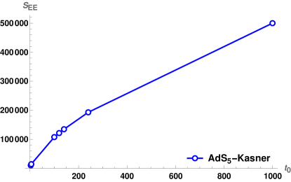
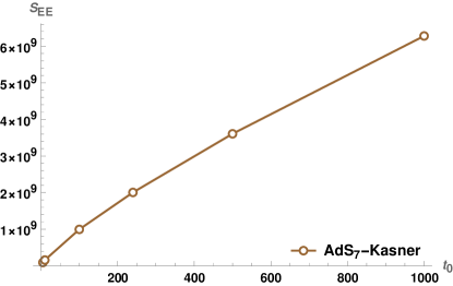
Figure 14: Numerical plots of holographic entanglement entropy versus $t_{0}$ for $AdS_{5,7}$-Kasner.

This indicates that entanglement entropy in AdS-Kasner spacetime decreases as $t_{0}$ decreases, and eventually becomes zero when $t_{0}\rightarrow 0$. This is also consistent with what we observed in Fig. 12 where we see that the entangling surfaces $t(r)$ become lightlike earlier for anchoring time slice $t_{0}$ closer to the singularity.

We now compare the IR entangling RT/HRT surfaces for $AdS_{5}$-Kasner (Fig. 12) and $AdS_{7}$-Kasner (Fig. 13), as we had done for complexity surfaces in sec. 3.4. We see that the surfaces approach the lightlike regime earlier in $AdS_{7}$-Kasner relative to $AdS_{5}$-Kasner, similar to the complexity surfaces. Here again this appears to stem from the amplification factor ${1\over r^{d_{i}-1}}$ of the lightlike factor $\sqrt{1-(t^{\prime})^{2}}$ in entanglement entropy, so the effective thinning of the degrees of freedom is more rapid in higher dimensions.

As a mathematical observation, by comparing the $t(r)$ plots in $AdS$-Kasner, we see that the complexity surfaces become lightlike earlier than the entangling RT/HRT surfaces. This can be seen to follow from the equations of motion which are similar in structure but differ in the numerical factors that appear: for $AdS_{5}$-Kasner, we have from (7.3), (3.3),

$$1-(t^{\prime})^{2}={{3\over 2}r\,t\,t^{\prime\prime}\over{9\over 2}t\,t^{\prime}-r}\ \ \ [{\rm EE}]\,;\qquad 1-(t^{\prime})^{2}={r\,t\,t^{\prime\prime}\over 4t\,t^{\prime}-r}\ \ \ [{\rm complexity}]\,.$$ (7.8)

the denominator factors are comparable so the relative factor of ${3\over 2}$ makes $(1-(t^{\prime})^{2})$ larger so $t^{\prime}(r)$ is smaller for the entangling surface $t(r)$.

Explicit expressions for holographic entanglement entropy (6.3) can be obtained for hyperscaling violating cosmologies using (4). The exponents for $t(r)$ are fairly nontrivial. The $r$-scalings give the leading divergence as $S_{EE}\sim{V_{d_{i}-1}\over G_{d_{i}+2}}\,{R^{d_{i}-\theta}\over\epsilon^{d_{i}-\theta-1}}$ where we have reinstated the dimensionful bulk scale $R$ (which can be done simply on dimensional grounds). This can be recast as

$$S_{EE}\sim{V_{d_{i}-1}\over G_{d_{i}+2}}\,{R^{d_{i}-\theta}\over\epsilon^{d_{i}-\theta-1}}\ \sim\ N_{eff}(\epsilon)\,{V_{d_{i}-1}\over\epsilon^{d_{i}-1}}\,,\qquad N_{eff}(\epsilon)={R^{d_{i}-\theta}\over G_{d_{i}+2}}\,\epsilon^{\theta}\,,$$ (7.9)

where $N_{eff}$ is the effective scale-dependent number of degrees of freedom evaluated at the UV cutoff length $\epsilon$ (see [91], [102]). In concrete gauge/string realizations of hyperscaling violating theories obtained by dimensional reduction of nonconformal $Dp$-branes, it can be seen that the lengthscales in the $Dp$-brane description reorganize themselves as the above and also match various expectations, including from considerations of the holographic c-function from a 2-dim dilaton gravity point of view [96]. For instance, the $d_{i}=2,\ \theta=-{1\over 3}$ case corresponding to the D2-brane supergravity phase with $G_{4}\sim{G_{10}\over R^{6}}$ after the transverse sphere reduction gives $N_{eff}=N^{2}\,(g_{YM}^{2}N\epsilon)^{-1/3}$ which ends up being consistent with the regime of validity of the D2-supergravity phase. By comparison the complexity scalings then are less obvious. The leading divergence of complexity in hyperscaling violating theories can be expressed as

$$C\ \sim\ {V_{d_{i}}\over G_{d_{i}+2}}\,\Big{(}{R\over\epsilon}\Big{)}^{d_{i}-\theta-{\theta\over d_{i}}}\ \sim\ N_{eff}(\epsilon)\,{V_{d_{i}}\over\epsilon^{d_{i}}}\,\Big{(}{R\over\epsilon}\Big{)}^{\!\!\!{}^{-{\theta\over d_{i}}}}\,,$$ (7.10)

using $N_{eff}$ in (7.9). The extra factor $({R\over\epsilon})^{{-\theta\over d_{i}}}$ arising from the extra metric factor for codim-1 surfaces (relative to codim-2) cannot be obviously recast in terms of field theory parameters once $N_{eff}$ is pulled out (see [22, 24, 46, 60] for other complexity studies). Of course this can be expressed in terms of some effective UV cutoff ${\tilde{\Lambda}}^{d_{i}-{\theta\over d_{i}}}\,R^{-{\theta\over d_{i}}}$. The scalings of complexity with time are also nontrivial. It would be interesting to understand this better.

The numerical plots of the entangling RT/HRT surfaces for the hyperscaling violating cosmology with $d_{i}=4,\ \theta=-1$ are qualitatively similar to the above for sufficiently high $t_{0}$: away from this, there appear to be some numerical issues (as well as for the $d_{i}=2,\ \theta=-{1\over 3}$ case), similar to the $AdS_{4}$ Kasner case stated earlier. So we do not discuss these in detail.

8 Discussion

We have studied holographic volume complexity and entanglement entropy in various families of cosmologies with Big-Bang/Crunch singularities, some of which were studied previously in e.g. [77]-[84]. These include $AdS$, hyperscaling violating and Lifshitz asymptotics. Focussing on isotropic Kasner-like singularities, we saw that higher dimensional complexity and entanglement can be recast in terms of that in 2-dimensional dilaton gravity theories obtained by dimensional reduction [95], and the resulting expressions are compactly written in terms of entirely 2-dim variables.

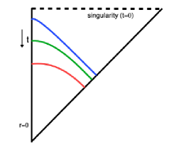
Figure 15: Cartoon of complexity and IR entanglement surfaces at various anchoring time slices $t$ on the boundary ($r=0$) in holographic cosmologies with Kasner-like Big-Crunch singularities. The extremal surfaces bend away from the singularity (dotted line, $t=0$) and approach lightlike regimes eventually (approaching faster as $t\rightarrow 0$).

The equation of motion for the complexity and IR entangling surfaces obtained by extremization of the complexity and entanglement functionals can be solved perturbatively near the holographic boundary: using this allows us to extract boundary conditions for numerical solutions of the surfaces. In the numerics, we impose a near-boundary cutoff $\epsilon$: the interior end approaches a lightlike regime so no interior regulator is required. The complexity plots appear in Figs. 2-3, 4, 5 for $AdS_{5,4,7}$ Kasner, Figs. 7, 8 for hyperscaling violating cosmologies, and Fig. 10 for Lifshitz Kasner, and those of entanglement appear in Fig. 12, Fig. 13 for $AdS_{5,7}$ Kasner.

Overall this shows that the surfaces begin spacelike near the boundary, bend in the direction away from the location of the singularity and transition to lightlike in the interior (sec. 3.1.1). For instance in (7.8), (i) with $(t^{\prime})^{2}\ll 1$ (spacelike), we see by using a series expansion for $t(r)$ that $t^{\prime}(r)>0$, and (ii) with $1-(t^{\prime})^{2}\sim 0^{+}$ (lightlike), we see that $t^{\prime\prime}>0$. As the anchoring time slice is moved towards the singularity, the spacelike part shrinks and the transition to lightlike is more rapid. The overall picture depicting a future Big-Crunch singularity is shown in Fig. 15 above (which is top-bottom reflected relative to the plots): note that $t\equiv|t|$ here so our analysis applies equally well to past Big-Bang singularities (e.g. in (7.8), $t\rightarrow-t$ is a symmetry). The complexity and entanglement functionals contain a $\sqrt{1-(t^{\prime})^{2}}$ factor so that the lightlike regimes give vanishing contributions: see Figs. 6, 9, 11 (complexity) and Fig. 14 (EE). Thus the near singularity region has vanishingly low complexity and entanglement and the “dual Kasner state” in all these theories corresponds to the effective number of qubits being vanishingly low, consistent with spatial volumes undergoing a Crunch. Our results corroborate those in [11] for volume complexity, and in [54] from holographic path integral optimization, in $AdS$ Kasner. However our analysis (in particular numerically) is more detailed and applies to various families of cosmologies which are in the same “universality class” in the scaling behaviour (2.6) near the singularity. Our entanglement analysis develops further the semiclassical perturbative study in [87], where the entangling surfaces were shown to bend away from the singularity (and quantum extremal surfaces are driven far away). Our numerics is consistent with the behaviour of entangling surfaces for finite subregions which only bend mildly (App. C).

It is worth noting that in the region very near the singularity, where the transition to lightlike is rapid, the anchoring time slice $t_{0}$ eventually becomes comparable to the cutoff $\epsilon$, i.e. $t_{0}\sim\epsilon$. At this point, it is perhaps best to say that the semiclassical gravity framework here becomes unreliable: so in concluding complexity to be vanishingly low as $t_{0}\rightarrow 0$, we are extrapolating the decreasing complexity to the very near singularity region. While this appears reasonable, it is worth understanding the very near singularity region more elaborately. At a very basic level, our analysis of holographic volume complexity and entanglement (building on those in [87, 88]) and those in [11], [54] (as well as the limiting surface in the black hole interior [89]) suggests that these sorts of spacelike Kasner cosmological singularities are excluded from the entanglement wedge of observers, as defined by the extremal surfaces that self-consistently steer clear of the vicinity of the singularity. This is a kind of “entanglement wedge cosmic censorship” (we thank Sumit Das for this phrase!). In some sense, this is reassuring since if it were not true, it would amount to a breakdown of the semiclassical gravity framework here, and thereby inconsistencies. Perhaps studying null singularities will reveal qualitatively new behaviour in light of the studies of the holographic duals in [78] and quantum extremal surfaces in [88] which bend towards the singularity.

We have focussed on the isotropic Kasner subfamily which is natural from the point of view of reduction to 2-dimensions. However it is likely that there are more general spacetimes with hyperscaling violating and Lifshitz asymptotics with general anisotropic Kasner singularities, analogous to the general anisotropic Kasner spacetimes in $AdS$. The constraint $\sum_{i}p_{i}=1$ would then imply that holographic volume complexity would be the same as in our analysis, although entanglement entropy, requiring a specification of the boundary spatial subregion would depend on the spatial orientation of the subregion.

More general $AdS$-BKL-type singularities were also studied in [80]. In these cases, spatial curvatures force BKL oscillations between various Kasner regimes (starting with some Kasner exponent negative), which continue indefinitely in the absence of external scalars [103, 104, 105]. In the presence of the scalar $\Psi$ as we have, the BKL oscillations lead to attractor-type basins eventually (with all Kasner exponents positive). Holographic entanglement requires defining a spatial subregion and thus would appear to evolve along BKL oscillations. Since the volume complexity functional for anisotropic $AdS$-Kasner backgrounds is similar, the evolution of complexity naively appears insensitive to these BKL oscillations, but it would be interesting to explore complexity more carefully to see the role of spatial curvatures.

The effectively 2-dim nature of our bulk analysis suggests effective dual 1-dim qubit models governing complexity. In $AdS$ and Lifshitz Kasner, the complexity decrease with time is linear whereas in hyperscaling violating theories, it is not. These latter theories with nonzero $\theta$ have effective spatial dimensions $d_{eff}=d_{i}-\theta$: it might be interesting to study effective 1-dim qubit models simulating this (recalling the general arguments in [3]).

Finally it is worth noting that the Kasner singularities we have been discussing have time dependence that does not switch off asymptotically. This reflects in the nontrivial Kasner scale $t_{K}$ lingering in our expressions: for instance (3.21) after reinstating $t_{K}$ is really $C\sim N_{dof}\,V_{d_{i}}\Lambda_{{}_{UV}}^{d_{i}}\,{t_{0}\over t_{K}}$ so this perhaps cannot be extrapolated to asymptotically large timescales $t_{0}\gg t_{K}$. The main merit of these models is the simplicity of the bulk in the vicinity of the singularity. Perhaps, as in [88] for quantum extremal surfaces, asymptotic regions with no time-dependence can be appended beyond $t_{0}>t_{K}$ with appropriate boundary conditions. In this case, the extremal surfaces becoming lightlike hitting the past horizon here (Fig. 15) must instead presumably be extended to these asymptotic far-regions (translating the question of the behaviour at the past horizon to the behaviour asymptotically). This hopefully will lead to better understanding of the (non-generic) initial conditions in the asymptotic regions that give rise to this “dual Kasner state” and its low complexity.

Acknowledgements:  We (especially KN) are particularly grateful to Sumit Das for very insightful early discusssions on low holographic complexity in the vicinity of cosmological singularities. We also thank Pawel Caputa, Abhijit Gadde, Alok Laddha, A. Manu and Rob Myers for useful discussions, and Sumit Das and Rob Myers for useful comments on a draft. GY would also like to thank Krishna Jalan, Pankaj Saini, Harsh Rana and Ashutosh Singh for helpful discussions about numerical calculations. GY would like to thank the Isaac Newton Institute for Mathematical Sciences for support and hospitality during the programme “Bridges between holographic quantum information and quantum gravity” while this work was in progress. We thank the organizers of the Indian Strings Meeting 2023 (ISM2023), IIT Bombay, for hospitality while this work was in progress. This work is partially supported by a grant to CMI from the Infosys Foundation and by EPSRC Grant Number EP/R0146014/1.

Appendix A Holographic cosmologies $\rightarrow$ 2-dim

Time-dependent non-normalizable deformations of $AdS/CFT$ were studied in [77, 78, 79, 80] towards gaining insights via gauge/gravity duality into cosmological (Big-Bang or -Crunch) singularities. The bulk gravity theory exhibits a cosmological Big-Crunch (or -Bang) singularity and breaks down while the holographic dual field theory (in the $AdS_{5}$ case) subject to a severe time-dependent gauge coupling $g_{YM}^{2}=e^{\Psi}$ (and living on a time-dependent base space) may be hoped to provide insight into the dual dynamics: in this case the scalar $\Psi$ controls the gauge/string coupling. There is a large family of such backgrounds exhibiting cosmological singularities. Among the simplest are $AdS$-Kasner theories

$$ds^{2}={R_{AdS}^{2}\over r^{2}}(-dt^{2}+\sum_{i}t^{2p_{i}}dx_{i}^{2}+dr^{2}),\quad e^{\Psi}=t^{\alpha}\ ;\qquad\sum_{i}p_{i}=1\ ,\quad\sum_{i}p_{i}^{2}=1-{1\over 2}\alpha^{2}\ .$$ (A1)

For constant scalar $\Psi$ with $\alpha=0$, the Kasner space is necessarily anisotropic: the $p_{i}$ cannot all be equal. In this case, the gauge theory lives on a time-dependent space but the gauge coupling is not time-dependent. The isotropic subfamily requires a nontrivial scalar source $\Psi$ as well. More general backgrounds can also be found involving $AdS$-FRW and $AdS$-BKL spacetimes [79, 80], all of which have spacelike singularities. There are also backgrounds with null singularities [78]. Similar Kasner deformations exist for $AdS_{4}\times X^{7}$ and $AdS_{7}\times X^{4}$. For generic spacelike singularities, the gauge theory response appears singular [80] while null singularities appear better behaved [78]. Some of these spacelike singularities were further investigated in [81, 82, 83, 84]

These arise in higher dimensional theories of Einstein gravity with scalar $\Psi$, a potential $V$, and action

$$S={1\over 16\pi G_{D}}\int d^{D}x\sqrt{-g^{(D)}}\,\Big{(}{\cal R}-{1\over 2}(\partial\Psi)^{2}-V\Big{)}\ .$$ (A2)

We allow the potential $V$ to also contain metric data, i.e. it is a function $V(g,\Psi)$. Under dimensional reduction with ansatz (2), we obtain the 2-dim action (2.4) (see the general reviews [97, 98, 99], of 2-dim dilaton gravity theories and dimensional reduction). In general these sorts of generic 2-dim dilaton gravity theories encapsulate various aspects of the higher dimensional gravity theories, and are perhaps best regarded as effective holographic models [94]. These sorts of theories were considered in [96] towards understanding holographic c-functions from the 2-dim dilaton gravity point of view. The 2-dim equations of motion following from (2.4) were solved in [95] with various families of asymptotics (flat, $AdS$, hyperscaling violating and Lifshitz) to obtain various classes of 2-dim cosmologies with Kasner-like Big-Bang/Crunch singularities.

We now review a little more from [95]. With $AdS$ asymptotics, we have $V=2\Lambda$ giving the dilaton potential in (2.4) as $U=2\Lambda\phi^{1/d_{i}}$ (3) independent of the scalar $\Psi$. Hyperscaling violating asymptotics $ds^{2}=\frac{{R^{2}}r^{2\theta/d_{i}}}{r^{2}}(-dt^{2}+dr^{2}+dx_{i}^{2})$ with nontrivial exponent $\theta$ arise [100] from dimensional reductions of nonconformal $Dp$-branes [101]: after reduction over the transverse sphere we obtain a $(d_{i}+2)$-dim action of the form (A2) with $V=2\Lambda\,e^{\gamma\Psi}$, which after reduction over the $d_{i}$ spatial dimensions gives (2.4) with $U$ in (4), and the corresponding parameters for the on-shell backgrounds. Lifshitz asymptotics $ds^{2}=R^{2}(-{dt^{2}\over r^{2z}}+{dr^{2}\over r^{2}}+{dx_{i}^{2}\over r^{2}})$ with nontrivial exponent $z$ requires a further gauge field strength, which on-shell leads to an action (A2) with effective potential of the form $V=\phi^{-1/d_{i}}U$ with $U$ in (5). Hyperscaling violating Lifshitz theories contain both nontrivial $z$ and $\theta$ exponents.

Cosmological deformations of the isotropic Kasner kind were found in [95] by solving the 2-dim theories obtained by reduction over the transverse $d_{i}$-space. The power law ansatz (2.5) for the 2-dim fields $\phi,\ e^{f},\ e^{\Psi}$ describes the vicinity of the singularity. The exponents, fixed by the 2-dim equations, with various asymptotics are in (3), (4) and (5). The asymptotics are the same as those in the absence of the time-dependence. For the $AdS$ and hyperscaling violating cases, the solutions for the $t$- and $r$-parts of the equations of motion end up being compatible (they are roughly independent). In general however, the time-dependent backgrounds are more constraining, particularly in the Lifshitz case where the equations couple the $t$- and $r$-exponents forcing $\theta=0$ and $z=d_{i}$.

As in $AdS_{5}$ Kasner, the scalar $e^{\Psi}$ controls the gauge coupling in nonconformal brane theories as well. Taking the exponent $\alpha>0$ in (4) amounts to taking the gauge coupling to vanish at $t=0$ which then leads to diverging $(\dot{\Psi})^{2}\sim{1\over t^{\#}}$ and thence a bulk singularity.

Appendix B $g_{i},s_{i},y_{i},v_{i}$

• $g_{2,4,...,30}$ appearing in (4.8) are given as:

  $$\hskip-43.36243ptg_{2}=\frac{15-2\sqrt{2}}{70t_{0}},\ \ \ g_{4}=\frac{5036\sqrt{2}-25835}{343000t_{0}^{3}},\ \ \ g_{6}=\frac{131312375-61266222\sqrt{2}}{7563150000t_{0}^{5}},\ \ \ g_{8}=\frac{118043488616\sqrt{2}-239576859153}{20753283600000t_{0}^{7}}$$

  $$\hskip-43.36243ptg_{10}=\frac{30641725271690815-18057721589949626\sqrt{2}}{4660841608500000000t_{0}^{9}},\ \ \ \ \ \ g_{12}=\frac{1746777870002066307428\sqrt{2}-2750377610449766429675}{616629344804550000000000t_{0}^{11}},$$

  $$\hskip-43.36243ptg_{14}=\frac{128643093652585740530239043-85306527498261677828242878\sqrt{2}}{40185734400912523500000000000t_{0}^{13}},$$

  $$\hskip-43.36243ptg_{16}=\frac{49284423774482049604693770127856\sqrt{2}-72262257714101067994459020233475}{30192881779885609323000000000000000t_{0}^{15}},$$

  $$\hskip-43.36243ptg_{18}=\frac{19995439034495716019982821920572548805-13839692268959015093440710251217475942\sqrt{2}}{10785199300592938506268830000000000000000t_{0}^{17}},$$

  $$\hskip-43.36243ptg_{20}=\frac{92461734333974336433412036570004178022497924\sqrt{2}-132383233749518151202669436990697126658121725}{90104947556803704750622940235000000000000000000t_{0}^{19}},$$

  $$\hskip-43.36243ptg_{22}=\frac{1}{1133219890439401260080334511688850000000000000000000t_{0}^{21}}\Biggl{(}1344723251595656108454760770119508822103294408067$$

  $$-944062670806348852667149876630981093710769426102\sqrt{2}\Biggr{)},$$

  $$\hskip-43.36243ptg_{24}=\frac{1}{2784321270809608896017381895219504450000000000000000000000t_{0}^{23}}$$

  $$\hskip-43.36243pt\times\Biggl{(}1906929530945636667174205717477953799585369699888014616\sqrt{2}-2708092485387409840625480950913094187387860907547500965\Biggr{)},$$

  $$\hskip-43.36243ptg_{26}=\frac{1}{26692870375061099044784237622185106236482500000000000000000000000t_{0}^{25}}$$

  $$\hskip-43.36243pt\times\Biggl{(}21537715543683174657204903469047177034720772836796345805054475$$

  $$\hskip-43.36243pt-15192569536698308027179683087287238752036460541099784416057074\sqrt{2}\Biggr{)},$$

  $$\hskip-43.36243ptg_{28}=\frac{1}{3633777556893706478363718755305633713390379230000000000000000000000000t_{0}^{27}}$$

  $$\hskip-43.36243pt\Biggl{(}1734826636729295474006107514952927659894462062211456520001571113716\sqrt{2}$$

  $$\hskip-43.36243pt-2456881300059835791367820912650011039518022308653523249580314121539\Biggr{)},$$

  $$\hskip-43.36243ptg_{30}=\frac{1}{306477341370361321518293994470921279429486322232237500000000000000000000000000t_{0}^{29}}$$

  $$\hskip-43.36243pt\Biggl{(}175119458492254422635835328099075014573047816696529800863555239186981548395$$

  $$\hskip-43.36243pt-123726552138838445517607197454484769607254798470947448964597915937595803454\sqrt{2}\Biggr{)}.$$ (B1)

• $s_{2,4,...,30}$ appearing in (4.10) are given as:

  $$s_{2}=\frac{15-2\sqrt{2}}{70t_{0}},\ \ \ s_{4}=\frac{-233-60\sqrt{2}}{1960t_{0}^{3}},\ \ \ s_{6}=\frac{1366\sqrt{2}-3735}{176400t_{0}^{5}},\ \ \ s_{8}=-\frac{73\left(27960\sqrt{2}-61489\right)}{2420208000t_{0}^{7}}$$

  $$s_{10}=\frac{1703\left(542378\sqrt{2}-1034175\right)}{3105933600000t_{0}^{9}},\ \ \ \ \ \ s_{12}=-\frac{1873\left(10204020\sqrt{2}-17682137\right)}{335440828800000t_{0}^{11}}$$

  $$s_{14}=\frac{837181\left(188424574\sqrt{2}-306048135\right)}{7286892937632000000t_{0}^{13}},\ \ \ s_{16}=-\frac{3653627\left(3438464880\sqrt{2}-5344420321\right)}{2844096395051520000000t_{0}^{15}},$$

  $$s_{18}=\frac{127272373093\left(62265813842\sqrt{2}-93920164335\right)}{4789429888302809164800000000t_{0}^{17}},$$

  $$s_{20}=-\frac{27070628490967\left(1121827536300\sqrt{2}-1657865720393\right)}{103930628576170958876160000000000t_{0}^{19}},$$

  $$s_{22}=\frac{10643485661067019\left(20143144485286\sqrt{2}-29355295951095\right)}{2054015656093725383922508800000000000t_{0}^{21}},$$

  $$s_{24}=-\frac{710398428691759571\left(360857759181480\sqrt{2}-520902017207569\right)}{40373731736178266146380832972800000000000t_{0}^{23}},$$

  $$s_{26}=\frac{365432484780076077223\left(6454670422137338\sqrt{2}-9256961294839455\right)}{1579824122836655554307881994225664000000000000t_{0}^{25}},$$

  $$s_{28}=\frac{28573985436423295860389\left(115333978921738980\sqrt{2}-164673101111141177\right)}{1155026969807243727482873724667207680000000000000t_{0}^{27}},$$

  $$s_{30}=-\frac{8235897084099976314853039901\left(2059355886048367054\sqrt{2}-2931432432354073575\right)}{14807295599422789644645868376649395720601600000000000000t_{0}^{29}}.$$

• $y_{2,4,...,30}$ appearing in (4.15) are given as:

  $$\hskip-65.04256pty_{2}=\frac{17}{210t_{0}},\ \ \ y_{4}=-\frac{597941}{120393000t_{0}^{3}},\ \ \ y_{6}=\frac{993708293}{1021025250000t_{0}^{5}},\ \ \ y_{8}=\frac{452798139285229}{5073066057150000000t_{0}^{7}}$$

  $$\hskip-65.04256pty_{10}=-\frac{7762666145527314499}{3116130825604387500000000t_{0}^{9}},\ \ \ \ \ \ y_{12}=\frac{778626364308431708373971}{2611006018773916286250000000000t_{0}^{11}},$$

  $$\hskip-65.04256pty_{14}=-\frac{14532317551343739394845037807}{57572682713964854111812500000000000t_{0}^{13}},$$

  $$\hskip-65.04256pty_{16}=\frac{134775937177098635383635361763279329}{6674631397760801396598870375000000000000000t_{0}^{15}},$$

  $$\hskip-65.04256pty_{18}=-\frac{23026943114302604040791691983451855971093}{6328551759786903844185218946056250000000000000000t_{0}^{17}},$$

  $$\hskip-65.04256pty_{20}=\frac{3153560678290033043737528126244908333453747429}{12559010967297110678785566998448628125000000000000000000t_{0}^{19}},$$

  $$\hskip-65.04256pty_{22}=-\frac{2159192492450981405518188033547537283347434932424989}{102267816989850917305506225642250538011406250000000000000000000t_{0}^{21}},$$

  $$\hskip-65.04256pty_{24}=\frac{10044933432452681640166603056867038209059439843583881641653}{14763197978584296690571728822509131616358185718750000000000000000000000t_{0}^{23}},$$

  $$\hskip-65.04256pty_{26}=\frac{8111278236683441225687293147544323280834383533436340537805141977}{5037941310191891245657602460681241164082230876523437500000000000000000000000t_{0}^{25}},$$

  $$\hskip-65.04256pty_{28}=-\frac{22037160006779407400520716180389739557445655926283992889975840229704635441}{105718678919927610825312834270405259139559457420182986566406250000000000000000000000000t_{0}^{27}},$$

  $$\hskip-65.04256pty_{30}=\frac{173010178914907020259747210679911185098889364844402198485720676752426015674107}{3885161450307339697830246659437393273378810060191724756315429687500000000000000000000000000t_{0}^{29}}.$$ (B3)

• $v_{2,4,...,30}$ appearing in (4.17) are given as:

  $$\hskip-50.58878ptv_{2}=\frac{17}{210t_{0}},\ \ \ \ \ \ \ v_{4}=-\frac{289}{54600t_{0}^{3}},\ \ \ \ \ \ \ v_{6}=\frac{230911}{171990000t_{0}^{5}},\ \ \ \ \ \ \ v_{8}=\frac{18625183}{48157200000t_{0}^{7}},$$

  $$\hskip-50.58878ptv_{10}=-\frac{1259413159}{7230803580000000t_{0}^{9}},\ \ \ \ \ \ \ \ \ \ \ \ \ \ \ \ \ \ \ \ \ \ \ \ \ \ \ \ \ \ \ \ \ v_{12}=-\frac{1734694671323}{173105437705200000000t_{0}^{11}},$$

  $$\hskip-50.58878ptv_{14}=\frac{253061333967336493}{29772404230917348000000000t_{0}^{13}},\ \ \ \ \ \ \ \ \ \ \ \ \ \ \ \ \ \ \ v_{16}=-\frac{51584567107605271589}{7578430167869870400000000000t_{0}^{15}},$$

  $$\hskip-50.58878ptv_{18}=\frac{5068334544021849260813761}{12581937117602594934192000000000000t_{0}^{17}},\ \ \ \ \ \ v_{20}=-\frac{1170102518798981446719357833}{26422067946965449361803200000000000000t_{0}^{19}},$$

  $$\hskip-50.58878ptv_{22}=\frac{377636130323445910502267424507071}{57216900065593857374820290256000000000000000t_{0}^{21}},$$

  $$\hskip-50.58878ptv_{24}=\frac{4285432206726577629693771016097656661}{28981504221224600637493973420469120000000000000000t_{0}^{23}},$$

  $$\hskip-50.58878ptv_{26}=-\frac{164736794499568213033911204893352612209843}{7754967504529349387249429054427195360000000000000000000t_{0}^{25}},$$

  $$\hskip-50.58878ptv_{28}=\frac{63412257716902548637422789548968065947269115503}{13246570193186762862336239745029269482230400000000000000000000t_{0}^{27}},$$

  $$\hskip-50.58878ptv_{30}=-\frac{8469320387430327716246598983844309952267116513058601}{4882023444698981452914021158030537267676013920000000000000000000000t_{0}^{29}}.$$ (B4)

Appendix C EE, finite subregions ($A\neq 0$), $AdS_{5}$ Kasner

Here we give a brief description of the entangling RT/HRT surface for finite subregions, i.e. finite $A$, developing numerically the studies in [87]. The equation of motion for the entangling RT/HRT surface for finite $A$ in $AdS_{5}$ Kasner spacetime is given by (7.1) with $d_{i}=3$. The perturbative solution of this equation is the same as (7.4) for $A=0$. For nonzero $A$, we solve numerically for $t(r)$ up to the turning point $r_{*}$ determined by the condition (see (6.4), (6.5))

$$A=\phi_{*}=\frac{t(r_{*})}{r_{*}^{d_{i}}}\,.$$ (C1)

The perturbative solution (7.4) simplifies (C1) with $d_{i}=3$ to

$$6Ar_{*}^{3}t_{0}-r_{*}^{2}-6t_{0}^{2}=0\,.$$ (C2)

This can be solved for $r_{*}$ (with one real solution) but in perturbation theory, it is consistent to take $r_{*}\sim At_{0}^{1/d_{i}}$ since $t(r_{*})\sim t_{0}$, i.e. the surface is approximately on the $t_{0}$ constant time slice (the surface bends very little, as we confirm below). The $t(r)$-equation (7.1) with $d_{i}=3$ is solved numerically for the boundary conditions extracted from the perturbative solution (7.4). The numerical solution for the surface only makes sense upto the turning point $r_{*}$. We illustrate this fixing $A=1$ so $r_{*}\sim t_{0}^{1/3}$ here, with the results plotted in Fig. 16. It is clear that the bending is always small, i.e. $t^{\prime}(r)\ll 1$ over the entire surface as expected: the $t^{\prime}(r)$ values in Fig. 16 are in approximate agreement with the semiclassical $t^{\prime}\sim{r\over 3t_{0}}$ in (7.4). No lightlike limit arises here as expected (see Fig. 1 of [88] for a qualitative picture of the surface). This shows consistency of our techniques and analysis throughout the paper where the numerics for complexity and entanglement for large subregions with $A=0$ (Fig. 12) exhibits clear lightlike limits.

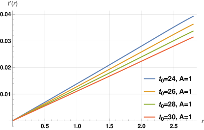
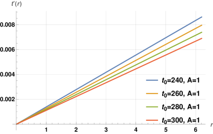
Figure 16: Numerical plots of $t^{\prime}(r)$ with $r$ in $AdS_{5}$ Kasner for different $t_{0}$ slices with $A=1$.

References

- [1]
- [2] J. Maldacena and L. Susskind, “Cool horizons for entangled black holes,” Fortsch. Phys. 61, 781-811 (2013) doi:10.1002/prop.201300020 [arXiv:1306.0533 [hep-th]].
- [3] L. Susskind, “Computational Complexity and Black Hole Horizons,” Fortsch. Phys. 64, 24-43 (2016) doi:10.1002/prop.201500092 [arXiv:1402.5674 [hep-th]], [arXiv:1403.5695 [hep-th]].
- [4] D. Stanford and L. Susskind, “Complexity and Shock Wave Geometries,” Phys. Rev. D 90, no.12, 126007 (2014) doi:10.1103/PhysRevD.90.126007 [arXiv:1406.2678 [hep-th]].
- [5] L. Susskind and Y. Zhao, “Switchbacks and the Bridge to Nowhere,” [arXiv:1408.2823 [hep-th]].
- [6] D. A. Roberts, D. Stanford and L. Susskind, “Localized shocks,” JHEP 03, 051 (2015) doi:10.1007/JHEP03(2015)051 [arXiv:1409.8180 [hep-th]].
- [7] L. Susskind, “Entanglement is not enough,” Fortsch. Phys. 64, 49-71 (2016) doi:10.1002/prop.201500095 [arXiv:1411.0690 [hep-th]].
- [8] L. Susskind, “The Typical-State Paradox: Diagnosing Horizons with Complexity,” Fortsch. Phys. 64, 84-91 (2016) doi:10.1002/prop.201500091 [arXiv:1507.02287 [hep-th]].
- [9] M. Alishahiha, “Holographic Complexity,” Phys. Rev. D 92, no.12, 126009 (2015) doi:10.1103/PhysRevD.92.126009 [arXiv:1509.06614 [hep-th]].
- [10] A. R. Brown, D. A. Roberts, L. Susskind, B. Swingle and Y. Zhao, “Holographic Complexity Equals Bulk Action?,” Phys. Rev. Lett. 116, no.19, 191301 (2016) doi:10.1103/PhysRevLett.116.191301 [arXiv:1509.07876 [hep-th]].
- [11] J. L. Barbon and E. Rabinovici, “Holographic complexity and spacetime singularities,” JHEP 01, 084 (2016) doi:10.1007/JHEP01(2016)084 [arXiv:1509.09291 [hep-th]].
- [12] A. R. Brown, D. A. Roberts, L. Susskind, B. Swingle and Y. Zhao, “Complexity, action, and black holes,” Phys. Rev. D 93, no.8, 086006 (2016) doi:10.1103/PhysRevD.93.086006 [arXiv:1512.04993 [hep-th]].
- [13] R. Q. Yang, “Strong energy condition and complexity growth bound in holography,” Phys. Rev. D 95, no.8, 086017 (2017) doi:10.1103/PhysRevD.95.086017 [arXiv:1610.05090 [gr-qc]].
- [14] H. Huang, X. H. Feng and H. Lu, “Holographic Complexity and Two Identities of Action Growth,” Phys. Lett. B 769, 357-361 (2017) doi:10.1016/j.physletb.2017.04.011 [arXiv:1611.02321 [hep-th]].
- [15] D. Carmi, R. C. Myers and P. Rath, “Comments on Holographic Complexity,” JHEP 03, 118 (2017) doi:10.1007/JHEP03(2017)118 [arXiv:1612.00433 [hep-th]].
- [16] A. Reynolds and S. F. Ross, “Divergences in Holographic Complexity,” Class. Quant. Grav. 34, no.10, 105004 (2017) doi:10.1088/1361-6382/aa6925 [arXiv:1612.05439 [hep-th]].
- [17] P. Caputa, N. Kundu, M. Miyaji, T. Takayanagi and K. Watanabe, “Anti-de Sitter Space from Optimization of Path Integrals in Conformal Field Theories,” Phys. Rev. Lett. 119, no.7, 071602 (2017) doi:10.1103/PhysRevLett.119.071602 [arXiv:1703.00456 [hep-th]].
- [18] S. Chapman, M. P. Heller, H. Marrochio and F. Pastawski, “Toward a Definition of Complexity for Quantum Field Theory States,” Phys. Rev. Lett. 120, no.12, 121602 (2018) doi:10.1103/PhysRevLett.120.121602 [arXiv:1707.08582 [hep-th]].
- [19] D. Carmi, S. Chapman, H. Marrochio, R. C. Myers and S. Sugishita, “On the Time Dependence of Holographic Complexity,” JHEP 11, 188 (2017) doi:10.1007/JHEP11(2017)188 [arXiv:1709.10184 [hep-th]].
- [20] W. Cottrell and M. Montero, “Complexity is simple!,” JHEP 02, 039 (2018) doi:10.1007/JHEP02(2018)039 [arXiv:1710.01175 [hep-th]].
- [21] J. Couch, S. Eccles, W. Fischler and M. L. Xiao, “Holographic complexity and noncommutative gauge theory,” JHEP 03, 108 (2018) doi:10.1007/JHEP03(2018)108 [arXiv:1710.07833 [hep-th]].
- [22] B. Swingle and Y. Wang, “Holographic Complexity of Einstein-Maxwell-Dilaton Gravity,” JHEP 09, 106 (2018) doi:10.1007/JHEP09(2018)106 [arXiv:1712.09826 [hep-th]].
- [23] S. Bolognesi, E. Rabinovici and S. R. Roy, “On Some Universal Features of the Holographic Quantum Complexity of Bulk Singularities,” JHEP 06, 016 (2018) doi:10.1007/JHEP06(2018)016 [arXiv:1802.02045 [hep-th]].
- [24] M. Alishahiha, A. Faraji Astaneh, M. R. Mohammadi Mozaffar and A. Mollabashi, “Complexity Growth with Lifshitz Scaling and Hyperscaling Violation,” JHEP 07, 042 (2018) doi:10.1007/JHEP07(2018)042 [arXiv:1802.06740 [hep-th]].
- [25] C. A. Agón, M. Headrick and B. Swingle, “Subsystem Complexity and Holography,” JHEP 02, 145 (2019) doi:10.1007/JHEP02(2019)145 [arXiv:1804.01561 [hep-th]].
- [26] A. Bhattacharyya, P. Caputa, S. R. Das, N. Kundu, M. Miyaji and T. Takayanagi, “Path-Integral Complexity for Perturbed CFTs,” JHEP 07, 086 (2018) doi:10.1007/JHEP07(2018)086 [arXiv:1804.01999 [hep-th]].
- [27] S. Chapman, H. Marrochio and R. C. Myers, “Holographic complexity in Vaidya spacetimes. Part I,” JHEP 06, 046 (2018) doi:10.1007/JHEP06(2018)046 [arXiv:1804.07410 [hep-th]].
- [28] P. Caputa and J. M. Magan, “Quantum Computation as Gravity,” Phys. Rev. Lett. 122, no.23, 231302 (2019) doi:10.1103/PhysRevLett.122.231302 [arXiv:1807.04422 [hep-th]].
- [29] H. A. Camargo, P. Caputa, D. Das, M. P. Heller and R. Jefferson, “Complexity as a novel probe of quantum quenches: universal scalings and purifications,” Phys. Rev. Lett. 122, no.8, 081601 (2019) doi:10.1103/PhysRevLett.122.081601 [arXiv:1807.07075 [hep-th]].
- [30] S. Chapman, J. Eisert, L. Hackl, M. P. Heller, R. Jefferson, H. Marrochio and R. C. Myers, “Complexity and entanglement for thermofield double states,” SciPost Phys. 6, no.3, 034 (2019) doi:10.21468/SciPostPhys.6.3.034 [arXiv:1810.05151 [hep-th]].
- [31] A. R. Brown, H. Gharibyan, H. W. Lin, L. Susskind, L. Thorlacius and Y. Zhao, “Complexity of Jackiw-Teitelboim gravity,” Phys. Rev. D 99, no.4, 046016 (2019) doi:10.1103/PhysRevD.99.046016 [arXiv:1810.08741 [hep-th]].
- [32] A. Akhavan, M. Alishahiha, A. Naseh and H. Zolfi, “Complexity and Behind the Horizon Cut Off,” JHEP 12, 090 (2018) doi:10.1007/JHEP12(2018)090 [arXiv:1810.12015 [hep-th]].
- [33] A. Belin, A. Lewkowycz and G. Sárosi, “Complexity and the bulk volume, a new York time story,” JHEP 03, 044 (2019) doi:10.1007/JHEP03(2019)044 [arXiv:1811.03097 [hep-th]].
- [34] S. Chapman, D. Ge and G. Policastro, “Holographic Complexity for Defects Distinguishes Action from Volume,” JHEP 05, 049 (2019) doi:10.1007/JHEP05(2019)049 [arXiv:1811.12549 [hep-th]].
- [35] K. Goto, H. Marrochio, R. C. Myers, L. Queimada and B. Yoshida, “Holographic Complexity Equals Which Action?,” JHEP 02, 160 (2019) doi:10.1007/JHEP02(2019)160 [arXiv:1901.00014 [hep-th]].
- [36] A. Bernamonti, F. Galli, J. Hernandez, R. C. Myers, S. M. Ruan and J. Simón, “First Law of Holographic Complexity,” Phys. Rev. Lett. 123, no.8, 081601 (2019) doi:10.1103/PhysRevLett.123.081601 [arXiv:1903.04511 [hep-th]].
- [37] T. Ali, A. Bhattacharyya, S. S. Haque, E. H. Kim, N. Moynihan and J. Murugan, “Chaos and Complexity in Quantum Mechanics,” Phys. Rev. D 101, no.2, 026021 (2020) doi:10.1103/PhysRevD.101.026021 [arXiv:1905.13534 [hep-th]].
- [38] R. J. Caginalp, “Holographic Complexity in FRW Spacetimes,” Phys. Rev. D 101, no.6, 066027 (2020) doi:10.1103/PhysRevD.101.066027 [arXiv:1906.02227 [hep-th]].
- [39] Y. S. An, R. G. Cai, L. Li and Y. Peng, “Holographic complexity growth in an FLRW universe,” Phys. Rev. D 101, no.4, 046006 (2020) doi:10.1103/PhysRevD.101.046006 [arXiv:1909.12172 [hep-th]].
- [40] P. Braccia, A. L. Cotrone and E. Tonni, “Complexity in the presence of a boundary,” JHEP 02, 051 (2020) doi:10.1007/JHEP02(2020)051 [arXiv:1910.03489 [hep-th]].
- [41] M. Doroudiani, A. Naseh and R. Pirmoradian, “Complexity for Charged Thermofield Double States,” JHEP 01, 120 (2020) doi:10.1007/JHEP01(2020)120 [arXiv:1910.08806 [hep-th]].
- [42] L. Schneiderbauer, W. Sybesma and L. Thorlacius, “Holographic Complexity: Stretching the Horizon of an Evaporating Black Hole,” JHEP 03, 069 (2020) doi:10.1007/JHEP03(2020)069 [arXiv:1911.06800 [hep-th]].
- [43] A. Bhattacharyya, S. Das, S. Shajidul Haque and B. Underwood, “Cosmological Complexity,” Phys. Rev. D 101, no.10, 106020 (2020) doi:10.1103/PhysRevD.101.106020 [arXiv:2001.08664 [hep-th]].
- [44] R. G. Cai, S. He, S. J. Wang and Y. X. Zhang, “Revisit on holographic complexity in two-dimensional gravity,” JHEP 08, 102 (2020) doi:10.1007/JHEP08(2020)102 [arXiv:2001.11626 [hep-th]].
- [45] A. Bhattacharyya, S. Das, S. S. Haque and B. Underwood, “Rise of cosmological complexity: Saturation of growth and chaos,” Phys. Rev. Res. 2, no.3, 033273 (2020) doi:10.1103/PhysRevResearch.2.033273 [arXiv:2005.10854 [hep-th]].
- [46] K. X. Zhu, F. W. Shu and D. H. Du, “Holographic complexity for nonlinearly charged Lifshitz black holes,” Class. Quant. Grav. 37, no.19, 195023 (2020) doi:10.1088/1361-6382/aba843 [arXiv:2007.11759 [hep-th]].
- [47] S. Choudhury, S. Chowdhury, N. Gupta, A. Mishara, S. P. Selvam, S. Panda, G. D. Pasquino, C. Singha and A. Swain, “Circuit Complexity from Cosmological Islands,” Symmetry 13, no.7, 1301 (2021) doi:10.3390/sym13071301 [arXiv:2012.10234 [hep-th]].
- [48] A. Bhattacharya, A. Bhattacharyya, P. Nandy and A. K. Patra, “Islands and complexity of eternal black hole and radiation subsystems for a doubly holographic model,” JHEP 05, 135 (2021) doi:10.1007/JHEP05(2021)135 [arXiv:2103.15852 [hep-th]].
- [49] S. Jiang and J. Jiang, “Holographic complexity in charged accelerating black holes,” Phys. Lett. B 823, 136731 (2021) doi:10.1016/j.physletb.2021.136731 [arXiv:2106.09371 [hep-th]].
- [50] N. Engelhardt and Å. Folkestad, “General bounds on holographic complexity,” JHEP 01, 040 (2022) doi:10.1007/JHEP01(2022)040 [arXiv:2109.06883 [hep-th]].
- [51] A. Bhattacharya, A. Bhattacharyya, P. Nandy and A. K. Patra, “Partial islands and subregion complexity in geometric secret-sharing model,” JHEP 12, 091 (2021) doi:10.1007/JHEP12(2021)091 [arXiv:2109.07842 [hep-th]].
- [52] S. Chapman, D. A. Galante and E. D. Kramer, “Holographic complexity and de Sitter space,” JHEP 02, 198 (2022) doi:10.1007/JHEP02(2022)198 [arXiv:2110.05522 [hep-th]].
- [53] A. Belin, R. C. Myers, S. M. Ruan, G. Sárosi and A. J. Speranza, “Does Complexity Equal Anything?,” Phys. Rev. Lett. 128, no.8, 081602 (2022) doi:10.1103/PhysRevLett.128.081602 [arXiv:2111.02429 [hep-th]].
- [54] P. Caputa, D. Das and S. R. Das, “Path integral complexity and Kasner singularities,” JHEP 01, 150 (2022) doi:10.1007/JHEP01(2022)150 [arXiv:2111.04405 [hep-th]].
- [55] R. Emparan, A. M. Frassino, M. Sasieta and M. Tomašević, “Holographic complexity of quantum black holes,” JHEP 02, 204 (2022) doi:10.1007/JHEP02(2022)204 [arXiv:2112.04860 [hep-th]].
- [56] E. Jørstad, R. C. Myers and S. M. Ruan, “Holographic complexity in dSd+1,” JHEP 05, 119 (2022) doi:10.1007/JHEP05(2022)119 [arXiv:2202.10684 [hep-th]].
- [57] K. Adhikari and S. Choudhury, “Cosmological Krylov Complexity,” Fortsch. Phys. 70, no.12, 2200126 (2022) doi:10.1002/prop.202200126 [arXiv:2203.14330 [hep-th]].
- [58] Y. S. An, L. Li, F. G. Yang and R. Q. Yang, “Interior structure and complexity growth rate of holographic superconductor from M-theory,” JHEP 08, 133 (2022) doi:10.1007/JHEP08(2022)133 [arXiv:2205.02442 [hep-th]].
- [59] T. Mandal, A. Mitra and G. S. Punia, “Action complexity of charged black holes with higher derivative interactions,” Phys. Rev. D 106, no.12, 126017 (2022) doi:10.1103/PhysRevD.106.126017 [arXiv:2205.11201 [hep-th]].
- [60] F. Omidi, “Generalized volume-complexity for two-sided hyperscaling violating black branes,” JHEP 01, 105 (2023) doi:10.1007/JHEP01(2023)105 [arXiv:2207.05287 [hep-th]].
- [61] S. Chapman, D. A. Galante, E. Harris, S. U. Sheorey and D. Vegh, “Complex geodesics in de Sitter space,” JHEP 03, 006 (2023) doi:10.1007/JHEP03(2023)006 [arXiv:2212.01398 [hep-th]].
- [62] R. Auzzi, G. Nardelli, G. P. Ungureanu and N. Zenoni, “Volume complexity of dS bubbles,” Phys. Rev. D 108, no.2, 026006 (2023) doi:10.1103/PhysRevD.108.026006 [arXiv:2302.03584 [hep-th]].
- [63] H. Zolfi, “Complexity and Multi-boundary Wormholes in 2 + 1 dimensions,” JHEP 04, 076 (2023) doi:10.1007/JHEP04(2023)076 [arXiv:2302.07522 [hep-th]].
- [64] G. Katoch, J. Ren and S. R. Roy, “Quantum complexity and bulk timelike singularities,” JHEP 12, 085 (2023) doi:10.1007/JHEP12(2023)085 [arXiv:2303.02752 [hep-th]].
- [65] T. Anegawa, N. Iizuka, S. K. Sake and N. Zenoni, “Is action complexity better for de Sitter space in Jackiw-Teitelboim gravity?,” JHEP 06, 213 (2023) doi:10.1007/JHEP06(2023)213 [arXiv:2303.05025 [hep-th]].
- [66] E. Jørstad, R. C. Myers and S. M. Ruan, “Complexity=anything: singularity probes,” JHEP 07, 223 (2023) doi:10.1007/JHEP07(2023)223 [arXiv:2304.05453 [hep-th]].
- [67] M. T. Wang, H. Y. Jiang and Y. X. Liu, “Generalized volume-complexity for RN-AdS black hole,” JHEP 07, 178 (2023) doi:10.1007/JHEP07(2023)178 [arXiv:2304.05751 [hep-th]].
- [68] A. Bhattacharya, A. Bhattacharyya and A. K. Patra, “Holographic complexity of Jackiw-Teitelboim gravity from Karch-Randall braneworld,” JHEP 07, 060 (2023) doi:10.1007/JHEP07(2023)060 [arXiv:2304.09909 [hep-th]].
- [69] T. Anegawa and N. Iizuka, “Shock waves and delay of hyperfast growth in de Sitter complexity,” JHEP 08, 115 (2023) doi:10.1007/JHEP08(2023)115 [arXiv:2304.14620 [hep-th]].
- [70] S. Baiguera, R. Berman, S. Chapman and R. C. Myers, “The cosmological switchback effect,” JHEP 07, 162 (2023) doi:10.1007/JHEP07(2023)162 [arXiv:2304.15008 [hep-th]].
- [71] S. E. Aguilar-Gutierrez, M. P. Heller and S. Van der Schueren, “Complexity = Anything Can Grow Forever in de Sitter,” [arXiv:2305.11280 [hep-th]].
- [72] G. Yadav and H. Rathi, “Yang-Baxter deformed wedge holography,” Phys. Lett. B 852, 138592 (2024) doi:10.1016/j.physletb.2024.138592 [arXiv:2307.01263 [hep-th]].
- [73] S. E. Aguilar-Gutierrez, A. K. Patra and J. F. Pedraza, “Entangled universes in dS wedge holography,” JHEP 10, 156 (2023) doi:10.1007/JHEP10(2023)156 [arXiv:2308.05666 [hep-th]].
- [74] S. E. Aguilar-Gutierrez, B. Craps, J. Hernandez, M. Khramtsov, M. Knysh and A. Shukla, “Holographic complexity: braneworld gravity versus the Lloyd bound,” [arXiv:2312.12349 [hep-th]].
- [75] S. E. Aguilar-Gutierrez, S. Baiguera and N. Zenoni, “Holographic complexity of the extended Schwarzschild-de Sitter space,” [arXiv:2402.01357 [hep-th]].
- [76] S. Chapman and G. Policastro, “Quantum computational complexity from quantum information to black holes and back,” Eur. Phys. J. C 82, no.2, 128 (2022) doi:10.1140/epjc/s10052-022-10037-1 [arXiv:2110.14672 [hep-th]].
- [77] S. R. Das, J. Michelson, K. Narayan and S. P. Trivedi, “Time dependent cosmologies and their duals,” Phys. Rev. D 74, 026002 (2006) [hep-th/0602107].
- [78] S. R. Das, J. Michelson, K. Narayan and S. P. Trivedi, “Cosmologies with Null Singularities and their Gauge Theory Duals,” Phys. Rev. D 75, 026002 (2007) [hep-th/0610053].
- [79] A. Awad, S. R. Das, K. Narayan and S. P. Trivedi, “Gauge theory duals of cosmological backgrounds and their energy momentum tensors,” Phys. Rev. D 77, 046008 (2008) [arXiv:0711.2994 [hep-th]].
- [80] A. Awad, S. Das, S. Nampuri, K. Narayan, S. Trivedi, “Gauge Theories with Time Dependent Couplings and their Cosmological Duals,” Phys.Rev.D79,046004(2009) [arXiv:0807.1517[hep-th]].
- [81] N. Engelhardt, T. Hertog and G. T. Horowitz, “Holographic Signatures of Cosmological Singularities,” Phys. Rev. Lett. 113, 121602 (2014) doi:10.1103/PhysRevLett.113.121602 [arXiv:1404.2309 [hep-th]].
- [82] N. Engelhardt, T. Hertog and G. T. Horowitz, “Further Holographic Investigations of Big Bang Singularities,” JHEP 1507, 044 (2015) doi:10.1007/JHEP07(2015)044 [arXiv:1503.08838 [hep-th]].
- [83] N. Engelhardt and G. T. Horowitz, “Holographic Consequences of a No Transmission Principle,” Phys. Rev. D 93, no.2, 026005 (2016) doi:10.1103/PhysRevD.93.026005 [arXiv:1509.07509 [hep-th]].
- [84] N. Engelhardt and G. T. Horowitz, “New Insights into Quantum Gravity from Gauge/gravity Duality,” Int. J. Mod. Phys. D 25, no.12, 1643002 (2016) doi:10.1142/S0218271816430021 [arXiv:1605.04335 [hep-th]].
- [85] B. Craps, “Big Bang Models in String Theory,” Class. Quant. Grav. 23, S849-S881 (2006) doi:10.1088/0264-9381/23/21/S01 [arXiv:hep-th/0605199 [hep-th]].
- [86] C. Burgess and L. McAllister, “Challenges for String Cosmology,” Class. Quant. Grav. 28, 204002 (2011) doi:10.1088/0264-9381/28/20/204002 [arXiv:1108.2660 [hep-th]].
- [87] A. Manu, K. Narayan and P. Paul, “Cosmological singularities, entanglement and quantum extremal surfaces,” JHEP 04, 200 (2021) doi:10.1007/JHEP04(2021)200 [arXiv:2012.07351 [hep-th]].
- [88] K. Goswami, K. Narayan and H. K. Saini, “Cosmologies, singularities and quantum extremal surfaces,” JHEP 03, 201 (2022) doi:10.1007/JHEP03(2022)201 [arXiv:2111.14906 [hep-th]].
- [89] T. Hartman and J. Maldacena, “Time Evolution of Entanglement Entropy from Black Hole Interiors,” JHEP 05, 014 (2013) doi:10.1007/JHEP05(2013)014 [arXiv:1303.1080 [hep-th]].
- [90] S. Ryu and T. Takayanagi, “Holographic derivation of entanglement entropy from AdS/CFT,” Phys. Rev. Lett. 96, 181602 (2006) [hep-th/0603001].
- [91] S. Ryu and T. Takayanagi, “Aspects of Holographic Entanglement Entropy,” JHEP 0608, 045 (2006) [hep-th/0605073].
- [92] V. E. Hubeny, M. Rangamani and T. Takayanagi, “A Covariant holographic entanglement entropy proposal,” JHEP 0707 (2007) 062 [arXiv:0705.0016 [hep-th]].
- [93] M. Rangamani and T. Takayanagi, “Holographic Entanglement Entropy,” Lect. Notes Phys. 931, pp.1 (2017) [arXiv:1609.01287 [hep-th]].
- [94] K. Narayan, “On aspects of two-dimensional dilaton gravity, dimensional reduction, and holography,” Phys. Rev. D 104, no.2, 026007 (2021) doi:10.1103/PhysRevD.104.026007 [arXiv:2010.12955 [hep-th]].
- [95] R. Bhattacharya, K. Narayan and P. Paul, “Cosmological singularities and 2-dimensional dilaton gravity,” JHEP 08, 062 (2020) doi:10.1007/JHEP08(2020)062 [arXiv:2006.09470 [hep-th]].
- [96] K. S. Kolekar and K. Narayan, “On AdS2 holography from redux, renormalization group flows and c-functions,” JHEP 02, 039 (2019) doi:10.1007/JHEP02(2019)039 [arXiv:1810.12528 [hep-th]].
- [97] A. Strominger, “Les Houches lectures on black holes,” [arXiv:hep-th/9501071 [hep-th]].
- [98] D. Grumiller, W. Kummer and D. V. Vassilevich, “Dilaton gravity in two-dimensions,” Phys. Rept. 369, 327-430 (2002) doi:10.1016/S0370-1573(02)00267-3 [arXiv:hep-th/0204253 [hep-th]].
- [99] T. G. Mertens and G. J. Turiaci, “Solvable models of quantum black holes: a review on Jackiw–Teitelboim gravity,” Living Rev. Rel. 26, no.1, 4 (2023) doi:10.1007/s41114-023-00046-1 [arXiv:2210.10846 [hep-th]].
- [100] X. Dong, S. Harrison, S. Kachru, G. Torroba and H. Wang, “Aspects of holography for theories with hyperscaling violation,” JHEP 06, 041 (2012) doi:10.1007/JHEP06(2012)041 [arXiv:1201.1905 [hep-th]].
- [101] N. Itzhaki, J. M. Maldacena, J. Sonnenschein and S. Yankielowicz, “Supergravity and the large N limit of theories with sixteen supercharges,” Phys. Rev. D 58, 046004 (1998) [hep-th/9802042].
- [102] J. L. F. Barbon and C. A. Fuertes, “Holographic entanglement entropy probes (non)locality,” JHEP 0804, 096 (2008) doi:10.1088/1126-6708/2008/04/096 [arXiv:0803.1928 [hep-th]].
- [103] L.D. Landau and E.M. Lifshitz, Course of Theoretical Physics, Vol. 2, “Classical Theory of Fields”, (Pergamon, 1987). This has a transparent treatment of the Bianchi classification of 4-dim cosmologies as well as the BKL analysis.
- [104] E. Lifshitz, V. Belinskii and I. Khalatnikov, Adv. Phys. 19 525(1970).
- [105] V. Belinskii and I. Khalatnikov, Sov. Phys. JETP 36 (1973) 591.