A compromise criterion for weighted least squares estimates

Jordan Bryan  
Haibo Zhou  
Didong Li  
Department of Biostatistics, University of North Carolina at Chapel Hill,
Chapel Hill, North Carolina 27599, U.S.A
Abstract

When independent errors in a linear model have non-identity covariance, the ordinary least squares estimate of the model coefficients is less efficient than the weighted least squares estimate. However, the practical application of weighted least squares is challenging due to its reliance on the unknown error covariance matrix. Although feasible weighted least squares estimates, which use an approximation of this matrix, often outperform the ordinary least squares estimate in terms of efficiency, this is not always the case. In some situations, feasible weighted least squares can be less efficient than ordinary least squares. The comparison between these two estimates has significant implications for the application of regression analysis in varied fields, yet such a comparison remains an unresolved challenge despite its seemingly straightforward nature. In this study, we directly address this challenge by identifying the conditions under which feasible weighted least squares estimates using fixed weights demonstrate greater efficiency than the ordinary least squares estimate. These conditions provide guidance for the design of feasible estimates using random weights. They also shed light on how certain robust regression estimates behave with respect to the linear model with normal errors of unequal variance.


Keywords: Heteroscedasticity; M-estimation; generalized variance.

1 Introduction

Using heteroscedasticity to improve the precision of regression estimates is an old, but not outdated practice. Indeed, modern statistical methods are still being adapted to incorporate information about heterogeneous variance in outcome variables. For instance, Shah et al. (2023) develop a consistent estimate of the error variance in a model for individualized treatment rules in order to stabilize their parameter estimates. In a different setting, Bryan et al. (2023) and Bryan and Hoff (2023) apply principles of variance estimation to devise more efficient estimates of water quality using fluorescence spectroscopy data. The question of how to address heteroscedasticity has continued to inspire new methodological developments primarily because, while classical least squares theory provides optimal estimates when the error variances are known, optimal procedures are more difficult to identify when the error variances must be estimated.

Such challenges arise even in the context of the standard linear model with independent errors:

$${\mathbf{y}}={\mathbf{X}}\boldsymbol{\beta}+\boldsymbol{\varepsilon},$$ (1)

where ${\mathbf{y}}\in\mathbb{R}^{n}$, ${\mathbf{X}}\in\mathbb{R}^{n\times p}$ is known and full-rank, and

$${\rm{E}}[\boldsymbol{\varepsilon}]={\mathbf{0}},~{}{\rm{Cov}}[\boldsymbol{\varepsilon}]={\rm{E}}[\boldsymbol{\varepsilon}\boldsymbol{\varepsilon}^{\top}]=\boldsymbol{\Omega}=\mathrm{diag}(\omega_{1},\dots,\omega_{n}).$$

In this setting, the weighted least squares estimate $({\mathbf{X}}^{\top}\boldsymbol{\Omega}^{-1}{\mathbf{X}})^{-1}{\mathbf{X}}^{\top}\boldsymbol{\Omega}^{-1}{\mathbf{y}}$ has minimum variance among all linear unbiased estimates of $\boldsymbol{\beta}$. However, computing the weighted least squares estimate requires knowledge of $\boldsymbol{\Omega}$, which is unknown in practice. By contrast, the ordinary least squares estimate $({\mathbf{X}}^{\top}{\mathbf{X}})^{-1}{\mathbf{X}}^{\top}{\mathbf{y}}$ can be computed in practice, since it is a function of ${\mathbf{X}}$ and ${\mathbf{y}}$ alone. Ordinary least squares, though, can be significantly less efficient than weighted least squares if there is a high degree of heteroscedasticity.

A so-called feasible weighted least squares estimate of $\boldsymbol{\beta}$ is obtained by plugging a computable estimate of $\boldsymbol{\Omega}$, denoted by $\tilde{\boldsymbol{\Omega}}$, into the vector-valued function $b_{{\mathbf{X}}}:\mathcal{D}_{+}^{n}\rightarrow\mathbb{R}^{p}$, defined as

$$b_{{\mathbf{X}}}(\tilde{\boldsymbol{\Omega}})=({\mathbf{X}}^{\top}\tilde{{\mathbf{\Omega}}}^{-1}{\mathbf{X}})^{-1}{\mathbf{X}}^{\top}\tilde{{\mathbf{\Omega}}}^{-1}{\mathbf{y}},$$ (2)

where $\mathcal{D}_{+}^{n}$ denotes the set of $n\times n$ diagonal positive definite matrices. This function yields the ordinary least squares estimate, $b_{{\mathbf{X}}}({\mathbf{I}}_{n})$, and the weighted least squares estimate, $b_{{\mathbf{X}}}(\boldsymbol{\Omega})$, as special cases. Feasible weighted least squares estimates have the benefit of being computable, and they have the potential to be more efficient than the ordinary least squares estimate. However, they also have the potential to be arbitrarily less precise than the ordinary least squares estimate if $\tilde{\boldsymbol{\Omega}}$, the feasible substitute for $\boldsymbol{\Omega}$, is far from the truth.

As only feasible and ordinary least squares estimates are available in practical settings, it is important to understand when the extra effort of designing feasible weights leads to a gain in efficiency relative to ordinary least squares. Interestingly, this question remains unresolved, despite the existence of an extensive statistical literature on its periphery. Classical works on this subject assess the efficiency of the ordinary least squares estimate (Anderson, 1948; Watson, 1967, 1972; Knott, 1975) or fixed-weight feasible weighted least squares estimates (Khatri and Rao, 1981; Wang and Yang, 1989) with respect to the efficiency of the optimal estimate $b_{{\mathbf{X}}}(\boldsymbol{\Omega})$. Likewise, Kurata and Kariya (1996) derive upper bounds for the variance of certain feasible weighted least squares estimates in terms of a scalar times the variance of the optimal $b_{{\mathbf{X}}}(\boldsymbol{\Omega})$.

A direct comparison between the efficiency of feasible and ordinary least squares, however, has remained elusive, seemingly for two distinct technical reasons. First, even in the case of fixed weights, directly comparing feasible and ordinary least squares involves three covariance matrices (the ground-truth $\boldsymbol{\Omega}$, the feasible weights $\tilde{\boldsymbol{\Omega}}$, and the identity ${\mathbf{I}}_{n}$) in such a way that appears to frustrate existing proof techniques for Kantorovich-type inequalities. Second, feasible weighted least squares estimates using random weights generally depend on ${\mathbf{y}}$ in a non-linear fashion, which makes explicit derivation of their covariance matrices difficult. For this reason, many contemporary approaches to feasible weighted least squares focus on designing random weights that are consistent for the true pattern of heteroscedasticity (Wooldridge, 2010; Wooldridge et al., 2016; Romano and Wolf, 2017), so that, in the limit, these estimates are efficient.

The approach taken in this article may be deemed a compromise between the classical and contemporary bodies of literature on weighted least squares. By overcoming some of the technical barriers above, we offer new insights into the comparison of feasible weighted least squares and ordinary least squares estimates. In particular, we characterize a class of feasible weighted least squares estimates, which are guaranteed to have lower variance than the ordinary least squares estimate in the case of a single regressor. In the case of multiple regressors, we show that this same class of estimates is guaranteed to outperform ordinary least squares in terms of generalized variance.

Following Bloomfield and Watson (1975), we define the generalized variance of a multivariate estimate as the determinant of its covariance matrix. For any feasible weighted least squares estimate that uses non-random weights $\tilde{\boldsymbol{\Omega}}$, the covariance matrix of $b_{{\mathbf{X}}}(\tilde{\boldsymbol{\Omega}})$ with respect to (1) will be an instance of the matrix-valued function $H_{{\mathbf{X}}}:\mathcal{D}_{+}^{n}\times\mathcal{D}_{+}^{n}\rightarrow\mathcal{S}_{+}^{p}$ defined as

$$H_{{\mathbf{X}}}(\tilde{\boldsymbol{\Omega}},\boldsymbol{\Omega})=({\mathbf{X}}^{\top}\tilde{\boldsymbol{\Omega}}^{-1}{\mathbf{X}})^{-1}{\mathbf{X}}^{\top}\tilde{\boldsymbol{\Omega}}^{-1}\boldsymbol{\Omega}\tilde{\boldsymbol{\Omega}}^{-1}{\mathbf{X}}({\mathbf{X}}^{\top}\tilde{\boldsymbol{\Omega}}^{-1}{\mathbf{X}})^{-1},$$ (3)

where $\mathcal{S}_{+}^{p}$ refers to the set of $p\times p$ positive definite matrices. The feasible weighted least squares estimates forming our subclass of interest therefore take the form

$$b_{{\mathbf{X}}}(\tilde{\boldsymbol{\Omega}}),~{}\tilde{\boldsymbol{\Omega}}\in\mathcal{C}^{p}_{\boldsymbol{\Omega}},$$

where

$$\mathcal{C}^{p}_{\boldsymbol{\Omega}}=\{\tilde{\boldsymbol{\Omega}}\in\mathcal{D}_{+}^{n}:|H_{{\mathbf{X}}}(\boldsymbol{\Omega},\boldsymbol{\Omega})|\leq|H_{{\mathbf{X}}}(\tilde{\boldsymbol{\Omega}},\boldsymbol{\Omega})|\leq|H_{{\mathbf{X}}}({\mathbf{I}}_{n},\boldsymbol{\Omega})|,~{}\forall{\mathbf{X}}\in\mathbb{R}^{n\times p}\}.$$ (4)

We call $\mathcal{C}^{p}_{\boldsymbol{\Omega}}$ a compromise set because its elements produce feasible weighted least squares estimates that are sub-optimal relative to the weighted least squares estimate, but are still preferable to the ordinary least squares estimate. That $\mathcal{C}^{p}_{\boldsymbol{\Omega}}$ is non-empty is guaranteed by a matrix Cauchy inequality (Marshall and Olkin, 1990), which says

$${\rm{Cov}}[b_{{\mathbf{X}}}({\mathbf{\Omega}})]=H_{{\mathbf{X}}}(\boldsymbol{\Omega},\boldsymbol{\Omega})\preceq H_{{\mathbf{X}}}({\mathbf{I}}_{n},\boldsymbol{\Omega})={\rm{Cov}}[b_{{\mathbf{X}}}({\mathbf{I}}_{n})],~{}\forall{\mathbf{X}}\in\mathbb{R}^{n\times p},$$

where $\preceq$ denotes the Loewner partial order on $\mathcal{S}_{+}^{p}$. In fact, a consequence of the Gauss-Markov Theorem (Aitken, 1936) is that $H_{{\mathbf{X}}}(\boldsymbol{\Omega},\boldsymbol{\Omega})\preceq H_{{\mathbf{X}}}(\tilde{\boldsymbol{\Omega}},\boldsymbol{\Omega}),~{}\forall{\mathbf{X}}\in\mathbb{R}^{n\times p},~{}\forall\tilde{\boldsymbol{\Omega}}\in\mathcal{D}_{n}^{+}$, so that $\mathcal{C}_{\boldsymbol{\Omega}}^{p}$ may be equivalently defined using only the second inequality in (4).

In Section 2 of this article, we examine the compromise set $\mathcal{C}^{p}_{\boldsymbol{\Omega}}$ in the case of a single regressor and provide a sufficient condition so that $\tilde{\boldsymbol{\Omega}}\in\mathcal{C}^{1}_{\boldsymbol{\Omega}}$. Building on this result, we then develop a necessary and sufficient condition so that $\tilde{\boldsymbol{\Omega}}\in\mathcal{C}^{p}_{\boldsymbol{\Omega}}$ for $1\leq p\leq n$. In Section 3 we discuss the implications of these results for estimation in the linear model. In particular, we show directly that a feasible weighted least squares estimate need not be consistent to outperform the ordinary least squares estimate. In Section 4, we provide a link between the results of Section 2 and the asymptotic variance of a robust regression estimate derived from the $t$-distribution. We then conduct numerical experiments in Section 5 that demonstrate how this estimate behaves in the context of the normal linear model with heteroscedasticity. In particular, we see that it behaves favorably relative to a parametric feasible weighted least squares estimate, especially for small sample sizes. Finally, in Section 6, we conclude with a discussion of possible extensions to this work. The proofs of all results may be found in Section A of the Appendix for this article.

2 Properties of compromise weights

The compromise set $\mathcal{C}^{p}_{\boldsymbol{\Omega}}$ is defined using the determinant inequality

$$|H_{{\mathbf{X}}}(\tilde{\boldsymbol{\Omega}},\boldsymbol{\Omega})|\leq|H_{{\mathbf{X}}}({\mathbf{I}}_{n},\boldsymbol{\Omega})|.$$ (5)

Because the determinant is invariant to multiplication of its matrix argument by any $p\times p$ orthogonal matrix, the inequality (5) is unchanged when ${\mathbf{U}}$, the matrix whose columns are the left singular vectors of ${\mathbf{X}}$, is substituted for ${\mathbf{X}}$ itself. In this section, it will be convenient to work in terms of ${\mathbf{U}}$ rather than ${\mathbf{X}}$.

To build intuition for the properties of compromise sets, consider the case of a single regressor so that $p=1$. Let $\mathcal{V}^{n}$ denote the set of $n$-dimensional unit vectors, write ${\mathbf{U}}\equiv{\mathbf{u}}\in\mathcal{V}^{n}$ and define the functions

$\displaystyle\mathrm{e}_{{\mathbf{u}}}(\boldsymbol{\Omega})$ $\displaystyle:=\sum_{i=1}^{n}u_{i}^{2}\omega_{i},$
$\displaystyle\mathrm{c}_{{\mathbf{u}}}(\tilde{\boldsymbol{\Omega}},\boldsymbol{\Omega})$ $\displaystyle:=\sum_{i=1}^{n}u_{i}^{2}(\tilde{\omega}_{i}-\mathrm{e}_{{\mathbf{u}}}(\tilde{\boldsymbol{\Omega}}))(\omega_{i}-\mathrm{e}_{{\mathbf{u}}}(\boldsymbol{\Omega})).$

Because ${\mathbf{u}}$ is a unit vector, the functions $\mathrm{e}_{{\mathbf{u}}}$ and $\mathrm{c}_{{\mathbf{u}}}$ behave, respectively, like the expectation and covariance functions of discrete random variables with supports determined by the diagonal entries of $\tilde{\boldsymbol{\Omega}},\boldsymbol{\Omega}$ and probability mass functions determined by ${\mathbf{u}}$. By rearranging terms in the inequality $H_{{\mathbf{u}}}(\tilde{\boldsymbol{\Omega}},\boldsymbol{\Omega})\leq H_{{\mathbf{u}}}({\mathbf{I}}_{n},\boldsymbol{\Omega})$, we can express the condition $\tilde{\boldsymbol{\Omega}}\in\mathcal{C}^{1}_{\boldsymbol{\Omega}}$ in terms of $\mathrm{e}_{{\mathbf{u}}}$ and $\mathrm{c}_{{\mathbf{u}}}$ as follows:

$$\tilde{\boldsymbol{\Omega}}\in\mathcal{C}^{1}_{\boldsymbol{\Omega}}\iff\mathrm{c}_{{\mathbf{u}}}(\tilde{\boldsymbol{\Phi}},\tilde{\boldsymbol{\Phi}}\boldsymbol{\Omega})+\mathrm{e}_{{\mathbf{u}}}(\tilde{\boldsymbol{\Phi}})\mathrm{c}_{{\mathbf{u}}}(\tilde{\boldsymbol{\Phi}},\boldsymbol{\Omega})\leq 0,~{}\forall{\mathbf{u}}\in\mathcal{V}^{n},$$ (6)

where $\tilde{\boldsymbol{\Phi}}=\tilde{\boldsymbol{\Omega}}^{-1}$. This formulation is useful because it points to an intuitive sufficient condition so that $\tilde{\boldsymbol{\Omega}}\in\mathcal{C}^{1}_{\boldsymbol{\Omega}}$, namely that both $\mathrm{c}_{{\mathbf{u}}}(\tilde{\boldsymbol{\Phi}},\tilde{\boldsymbol{\Phi}}\boldsymbol{\Omega})$ and $\mathrm{c}_{{\mathbf{u}}}(\tilde{\boldsymbol{\Phi}},\boldsymbol{\Omega})$ are non-positive for all ${\mathbf{u}}\in\mathcal{V}^{n}$. Now, for any ${\mathbf{u}}\in\mathcal{V}^{n}$, $\mathrm{c}_{{\mathbf{u}}}(\tilde{\boldsymbol{\Phi}},\boldsymbol{\Omega})$ will be non-positive if the diagonal entries of $\tilde{\boldsymbol{\Omega}}$ are in monotone non-decreasing relation with the diagonal entries of $\boldsymbol{\Omega}$ (Schmidt (2014), Corollary 3.1). The condition in the following proposition is sufficient so that $\mathrm{c}_{{\mathbf{u}}}(\tilde{\boldsymbol{\Phi}},\tilde{\boldsymbol{\Phi}}\boldsymbol{\Omega})$ is also non-positive for any choice of ${\mathbf{u}}$, implying that $\tilde{\boldsymbol{\Omega}}\in\mathcal{C}^{1}_{\boldsymbol{\Omega}}$.

Proposition 1.

For each $i\in\{1,\dots,n\}$ let $\tilde{\omega}_{i}=g(\omega_{i})$ where $g$ is a monotone non-decreasing function such that the function $f(\omega)=g(\omega)/\omega$ is monotone non-increasing. Then $\tilde{\boldsymbol{\Omega}}\in\mathcal{C}^{1}_{\boldsymbol{\Omega}}$.

In other words, for any ${\mathbf{u}}\in\mathcal{V}^{n}$, one is guaranteed that $H_{{\mathbf{u}}}(\tilde{\boldsymbol{\Omega}},\boldsymbol{\Omega})\leq H_{{\mathbf{u}}}({\mathbf{I}}_{n},\boldsymbol{\Omega})$ if the diagonal entries of $\tilde{\boldsymbol{\Omega}}$ grow monotonically, but not too quickly with the diagonal entries of $\boldsymbol{\Omega}$.

A function obeying the growth condition in Proposition 1 has a tapering effect on the extreme values of its inputs. Correspondingly, functions of this type have been used for robust covariance estimation (Maronna, 1976; Romanov et al., 2023), though in a different context than the one here. Some functions that satisfy this growth criterion are pictured in Figure 1. They include, but are not limited to, fractional powers ($g(\omega)=\omega^{1/q},~{}q\geq 1$) and translations by a positive constant ($g(\omega)=\omega+\lambda,~{}\lambda\in\mathbb{R}_{+}$). If $g$ is a function satisfying the growth criterion, then for non-negative constants $\lambda,\gamma$ the function

$$f(\omega)=\frac{1}{1/g(\omega)+\lambda}+\gamma$$ (7)

also satisfies it, where $f$ has the additional property of being bounded from above and below by $1/\lambda+\gamma$ and $\gamma$, respectively.

Refer to caption
Figure 1: Three functions satisfying the growth-restricted monotonicity condition in Proposition 1. From left to right, the functions are $\omega^{1/q}$, $1/\{\int_{-k}^{k}\mathrm{exp}(-z^{2}/2\omega)dz\}$, and $g_{1,\nu}(\omega)$, where this last function is defined in Theorem 2. For the purposes of visualization, the functions have been normalized to attain a maximum value of 1 at $\omega=10$.

The condition in Proposition 1 is too strong to provide a complete characterization of $\mathcal{C}^{1}_{\boldsymbol{\Omega}}$ because $\mathrm{c}_{{\mathbf{u}}}(\tilde{\boldsymbol{\Phi}},\tilde{\boldsymbol{\Phi}}\boldsymbol{\Omega})\leq 0,~{}\forall{\mathbf{u}}\in\mathcal{V}^{n}$ is not necessary for the right hand side of (6) to hold. However, the inequality

$\displaystyle\mathrm{c}_{{\mathbf{u}}}(\tilde{\boldsymbol{\Phi}},\tilde{\boldsymbol{\Phi}}\boldsymbol{\Omega})-\mathrm{e}_{{\mathbf{u}}}(\tilde{\boldsymbol{\Phi}})\mathrm{c}_{{\mathbf{u}}}(\tilde{\boldsymbol{\Phi}},\boldsymbol{\Omega})$ $\displaystyle=\mathrm{e}_{{\mathbf{u}}}(\tilde{\boldsymbol{\Phi}}^{2}\boldsymbol{\Omega})-\mathrm{e}_{{\mathbf{u}}}(\tilde{\boldsymbol{\Phi}})^{2}\mathrm{e}_{{\mathbf{u}}}(\boldsymbol{\Omega})$
$\displaystyle=\sum_{i=1}^{n}u_{i}^{2}\omega_{i}(\tilde{\phi}_{i}-\mathrm{e}_{{\mathbf{u}}}(\tilde{\boldsymbol{\Phi}}))^{2}$
$\displaystyle\geq 0$

demonstrates that $\mathrm{c}_{{\mathbf{u}}}(\tilde{\boldsymbol{\Phi}},\boldsymbol{\Omega})\leq 0,~{}\forall{\mathbf{u}}\in\mathcal{V}^{n}$ is necessary to ensure $\tilde{\boldsymbol{\Omega}}\in\mathcal{C}^{1}_{\boldsymbol{\Omega}}$. Thus, we should expect a necessary and sufficient condition for $\tilde{\boldsymbol{\Omega}}\in\mathcal{C}^{1}_{\boldsymbol{\Omega}}$ to include a monotonicity requirement on the diagonal entries of $\tilde{\boldsymbol{\Omega}}$ along with a weaker growth restriction than that of Proposition 1. The following theorem shows that this relaxed restriction can be expressed in terms of pairs of diagonal entries of $\tilde{\boldsymbol{\Omega}}$ and $\boldsymbol{\Omega}$.

Theorem 1.

Let $\boldsymbol{\Omega}=\mathrm{diag}(\omega_{1},\dots,\omega_{n})\in\mathcal{D}_{+}^{n}$ and let $\tilde{\boldsymbol{\Omega}}=\mathrm{diag}(\tilde{\omega}_{1},\dots,\tilde{\omega}_{n})\in\mathcal{D}_{+}^{n}$. Then $\tilde{\boldsymbol{\Omega}}\in\mathcal{C}^{1}_{\boldsymbol{\Omega}}$ if and only if

$$1\leq\frac{\tilde{\omega}_{i}}{\tilde{\omega}_{j}}\leq 2\frac{\omega_{i}}{\omega_{j}}-1$$ (8)

for all $\omega_{i}\geq\omega_{j}$, $i\in\{1,\dots,n\},j\in\{1,\dots,n\}$.

The elements of the proof of Theorem 1 may be combined with Hadamard’s determinant inequality (Marshall et al., 2011) to generalize the result to $\mathcal{C}^{p}_{\boldsymbol{\Omega}}$ for $p>1$.

Corollary 1.

Let $\boldsymbol{\Omega}=\mathrm{diag}(\omega_{1},\dots,\omega_{n})\in\mathcal{D}_{+}^{n}$ and let $\tilde{\boldsymbol{\Omega}}=\mathrm{diag}(\tilde{\omega}_{1},\dots,\tilde{\omega}_{n})\in\mathcal{D}_{+}^{n}$. Further, let $1\leq p\leq n$ and let $\tilde{\boldsymbol{\Omega}}=\mathrm{diag}(\tilde{\omega}_{1},\dots,\tilde{\omega}_{n})\in\mathcal{D}_{+}^{n}$. Then $\tilde{\boldsymbol{\Omega}}\in\mathcal{C}^{p}_{\boldsymbol{\Omega}}$ if and only if

$$1\leq\frac{\tilde{\omega}_{i}}{\tilde{\omega}_{j}}\leq 2\frac{\omega_{i}}{\omega_{j}}-1$$ (9)

for all $\omega_{i}\geq\omega_{j}$, $i\in\{1,\dots,n\},j\in\{1,\dots,n\}$.

We conclude this section by stating some properties of compromise weights that can be derived from Corollary 1. First, note that if the diagonal elements of $\tilde{\boldsymbol{\Omega}}$ satisfy the condition in Proposition 1, then $\tilde{\omega}_{i}/\tilde{\omega}_{j}\geq 1$ for all $\omega_{i}\geq\omega_{j}$, and $\tilde{\omega}_{i}\omega_{j}/(\tilde{\omega}_{j}\omega_{i})\leq 1\leq 2-(\omega_{j}/\omega_{i})$ for all $\omega_{i}\geq\omega_{j}$. Multiplying the latter inequalities by $\omega_{i}/\ \omega_{j}$ and comparing to (9) shows that Proposition 1 also applies to $p>1$. Next, because (9) depends only on pairwise ratios of diagonal elements, $\mathcal{C}^{p}_{\boldsymbol{\Omega}}$ has what Bilodeau (1990) and Kariya and Kurata (2004) call the “symmetric inverse property,” meaning

$$\tilde{\boldsymbol{\Omega}}\in\mathcal{C}^{p}_{\boldsymbol{\Omega}}\iff\tilde{\boldsymbol{\Omega}}^{-1}\in\mathcal{C}^{p}_{\boldsymbol{\Omega}^{-1}}.$$

Finally, $\mathcal{C}_{\boldsymbol{\Omega}}^{p}$ is a convex cone on $\mathcal{D}_{+}^{n}$. The cone property of $\mathcal{C}^{p}_{\boldsymbol{\Omega}}$ is clear from the fact that $H_{{\mathbf{X}}}(s\tilde{\boldsymbol{\Omega}},\boldsymbol{\Omega})=H_{{\mathbf{X}}}(\tilde{\boldsymbol{\Omega}},\boldsymbol{\Omega}),~{}\forall s>0$. The convexity of $\mathcal{C}^{p}_{\boldsymbol{\Omega}}$ can be derived directly from (9): given $\tilde{\boldsymbol{\Omega}},\tilde{\boldsymbol{\Psi}}\in\mathcal{C}^{p}_{\boldsymbol{\Omega}}$,

$$\tilde{\omega}_{j}\leq\tilde{\omega}_{i}\leq 2\frac{\omega_{i}}{\omega_{j}}\tilde{\omega}_{j}-\tilde{\omega}_{j},~{}\text{ and }~{}\tilde{\psi}_{j}\leq\tilde{\psi}_{i}\leq 2\frac{\omega_{i}}{\omega_{j}}\tilde{\psi}_{j}-\tilde{\psi}_{j}.$$

for all $\omega_{i}\geq\omega_{j}$. For any $0\leq t\leq 1$, this implies

$$t\tilde{\omega}_{j}+(1-t)\tilde{\psi}_{j}\leq t\tilde{\omega}_{i}+(1-t)\tilde{\psi}_{i}\leq 2\frac{\omega_{i}}{\omega_{j}}\{t\tilde{\omega}_{j}+(1-t)\tilde{\psi}_{j}\}-\{t\tilde{\omega}_{j}+(1-t)\tilde{\psi}_{j}\},$$

for all $\omega_{i}\geq\omega_{j}$, so $t\tilde{\boldsymbol{\Omega}}+(1-t)\tilde{\boldsymbol{\Psi}}\in\mathcal{C}^{p}_{\boldsymbol{\Omega}}$. Along with the cone property, convexity implies, among other things, that

$$\tilde{\boldsymbol{\Omega}}\in\mathcal{C}^{p}_{\boldsymbol{\Omega}}\implies\tilde{\boldsymbol{\Omega}}+s{\mathbf{I}}_{n}\in\mathcal{C}^{p}_{\boldsymbol{\Omega}},~{}\forall s>0,$$ (10)

so regularized compromise weights, in the sense of Ledoit and Wolf (2004), are also compromise weights.

3 Implications of compromise sets for estimation in the linear model

The matrix $H_{{\mathbf{X}}}(\tilde{\boldsymbol{\Omega}},\boldsymbol{\Omega})$ used to define the notion of a compromise set is equal to the covariance matrix of the feasible weighted least squares estimate $b_{{\mathbf{X}}}(\tilde{\boldsymbol{\Omega}})$ under (1) when $\tilde{\boldsymbol{\Omega}}$ is any fixed matrix in $\mathcal{D}_{n}^{+}$. As seen in the previous section, the conditions so that $\tilde{\boldsymbol{\Omega}}$ is a member of $\mathcal{C}^{p}_{\boldsymbol{\Omega}}$ depend on the unknown $\boldsymbol{\Omega}$. A natural question is then: to what extent is $b_{{\mathbf{X}}}(\tilde{\boldsymbol{\Omega}})$ actually feasible? More broadly, what is the relevance of Section 2 to estimation in practice if one must know $\boldsymbol{\Omega}$ to choose an appropriate $\tilde{\boldsymbol{\Omega}}$?

In fact, one does not need to know the values of the diagonal elements of $\boldsymbol{\Omega}$. One implication of Corollary 1 is that knowing the ranks of $(\omega_{1},\dots,\omega_{n})$ along with a lower bound on the minimum ratio between consecutive ordered elements $\gamma<\min_{i=j+1}\{\omega_{(i)}/\omega_{(j)}\}$ would be sufficient to construct an $\tilde{\boldsymbol{\Omega}}$ and a corresponding $b_{{\mathbf{X}}}(\tilde{\boldsymbol{\Omega}})$ that is guaranteed to outperform the ordinary least squares estimate. By contrast, to reproduce $\boldsymbol{\Omega}$ itself up to a scale factor, it would be necessary to know the ranks of the diagonal elements of $\boldsymbol{\Omega}$ along with the collection of all ratios between consecutive ordered elements. Thus, the task of finding an optimal estimate (the weighted least squares estimate) depends on more unknowns than the task of finding an estimate that is at least better than the ordinary least squares estimate.

This latter, more modest goal, brings otherwise impossible tasks into the feasible realm in certain simple cases. For instance, consider the groupwise heteroscedastic linear model with error covariance matrix

$$\boldsymbol{\Omega}=\boldsymbol{\Omega}(\boldsymbol{\sigma})=\left[\begin{array}[]{ccc}\sigma_{1}^{2}{\mathbf{I}}_{n_{1}}&&{\mathbf{0}}\\ &\ddots&\\ {\mathbf{0}}&&\sigma_{K}^{2}{\mathbf{I}}_{n_{K}}\end{array}\right],$$

where $\boldsymbol{\sigma}\in\mathbb{R}_{+}^{K}$, $n=\sum_{k=1}^{K}n_{k}$. While it is implausible that one knows the exact values of $\boldsymbol{\sigma}$ in advance, it seems at least more plausible that, for small $K$, one knows the ordering of the elements of $\boldsymbol{\sigma}$ and that no group’s error variance is within some factor $\gamma\geq 1$ of another’s. Let $\tilde{\sigma}_{(1)}^{2}=1$, and set $\tilde{\sigma}_{(i)}^{2}:=(2\gamma-1)\tilde{\sigma}_{(i-1)}^{2}$ for each $i>1$. Then, using the notation above, $\tilde{\boldsymbol{\Omega}}=\boldsymbol{\Omega}(\tilde{\boldsymbol{\sigma}})$ defines a matrix whose diagonal elements are compromise weights.

Alternatively, consider the linear model with error variances depending on a single covariate through a parameterized scedastic function

$$\omega_{i}=v_{\theta}(x_{i,1}),~{}i=1,\dots,n.$$

Common examples of $v_{\theta}$, all of which are used in the simulation studies of Romano and Wolf (2017), include

$\displaystyle v_{{\theta}}(x)$ $\displaystyle=|x|^{\theta}$ (11)
$\displaystyle v_{{\theta}}(x)$ $\displaystyle=\{\log(|x|)\}^{\theta}$
$\displaystyle v_{{\theta}}(x)$ $\displaystyle=e^{\theta|x|+\theta|x|^{2}}.$

Conveniently, in each specification above, the ranks of $(\omega_{1},\dots,\omega_{n})$ are equivalent to the ranks of $(x_{i,1},\dots,x_{n,1})$, which are known. Hence, if one can identify a lower bound $\gamma$ for the minimum plausible value of $\theta$, one can simply take $\tilde{\omega}_{i}=v_{\gamma}(x_{i,1})$, and the corresponding $b_{{\mathbf{X}}}(\tilde{\boldsymbol{\Omega}})$ will outperform the ordinary least squares estimate. This is due to the fact that, for each of the scedastic functions above, $\gamma\leq\theta$ implies that $v_{\gamma}(x)$ is a fractional power of $v_{\theta}(x)$ and thus satisfies the condition of Proposition 1.

With few exceptions (see Kariya and Kurata (2004)), feasible weighted least squares estimates using random weights will not have covariance matrix of the form (3). However, compromise sets may still act as target regions for such estimates in the asymptotic regime. Informally, if an estimate $\hat{\boldsymbol{\Omega}}_{n}$ is asymptotically equal to some $\tilde{\boldsymbol{\Omega}}\in\mathcal{C}^{p}_{{\mathbf{\Omega}}}$, then $b_{{\mathbf{X}}}(\hat{\boldsymbol{\Omega}}_{n})$ outperforms the ordinary least squares estimate if $n$ is large enough. In particular, $\hat{\boldsymbol{\Omega}}_{n}$ need not be consistent for $\boldsymbol{\Omega}$ in order to outperform ordinary least squares in the limit. Both Atkinson et al. (2016) and Romano and Wolf (2017) provide numerical evidence for this claim by evaluating the variance of feasible weighted least squares estimates when they are misspecified with respect to the true form of heteroscedasticity. Here, we give sufficient conditions on the probability limit of a feasible weighted least squares estimate $\hat{\boldsymbol{\Omega}}_{n}$ so that it outperforms the ordinary least squares estimate as $n\rightarrow\infty$. Since the dimension of $\boldsymbol{\Omega}$ grows with $n$, the statement of these conditions requires a slightly modified notation that replaces matrices with infinite sequences.

Proposition 2.

Given the sequences of positive scalars $\{\tilde{\omega}_{i}\}_{i=1}^{\infty}$, $\{\omega_{i}\}_{i=1}^{\infty}$, the sequence of $p$-dimensional vectors $\{{\mathbf{x}}_{i}\}_{i=1}^{\infty}$, and the sequence of random variables $\{y_{i}\}_{i=1}^{\infty}$, define the random estimate

$$\hat{\omega}_{i}=v_{\hat{\boldsymbol{\theta}}_{n}}({\mathbf{x}}_{i}),~{}i=1,\dots,n,$$

where $v_{\boldsymbol{\theta}}:\mathbb{R}^{p}\rightarrow\mathbb{R}_{+}$ is a fixed function and $\hat{\boldsymbol{\theta}}_{n}$ is a random finite-dimensional vector that depends on $\{{\mathbf{x}}_{i}\}_{i=1}^{n}$ and $\{y_{i}\}_{i=1}^{n}$. Assuming that

$$\lim_{n\rightarrow\infty}\frac{1}{n}\sum_{i=1}^{n}\frac{y_{i}}{\tilde{\omega}_{i}}{\mathbf{x}}_{i}~{}\text{ and }~{}\lim_{n\rightarrow\infty}\frac{1}{n}\sum_{i=1}^{n}\frac{1}{\tilde{\omega}_{i}}{\mathbf{x}}_{i}{\mathbf{x}}_{i}^{\top}~{}\text{ and }~{}\lim_{n\rightarrow\infty}\frac{1}{n}\sum_{i=1}^{n}\frac{\omega_{i}}{\tilde{\omega}^{2}_{i}}{\mathbf{x}}_{i}{\mathbf{x}}_{i}^{\top}$$

exist, define the coefficient estimates

$$b^{n}_{{\mathbf{X}}}(\{\tilde{\omega}_{i}\}_{i=1}^{\infty})=\left\{\frac{1}{n}\sum_{i=1}^{n}\frac{1}{\tilde{\omega}_{i}}{\mathbf{x}}_{i}{\mathbf{x}}_{i}^{\top}\right\}^{-1}\left\{\frac{1}{n}\sum_{i=1}^{n}\frac{y_{i}}{\tilde{\omega}_{i}}{\mathbf{x}}_{i}\right\}$$

and

$$b^{n}_{{\mathbf{X}}}(\{\hat{\omega}_{i}\}_{i=1}^{\infty})=\left\{\frac{1}{n}\sum_{i=1}^{n}\frac{1}{\hat{\omega}_{i}}{\mathbf{x}}_{i}{\mathbf{x}}_{i}^{\top}\right\}^{-1}\left\{\frac{1}{n}\sum_{i=1}^{n}\frac{y_{i}}{\hat{\omega}_{i}}{\mathbf{x}}_{i}\right\},$$

and suppose that $\{\hat{\omega}_{i}\}_{i=1}^{\infty}$ satisfies

$\displaystyle\frac{1}{n}\sum_{i=1}^{n}(1/\hat{\omega}_{i}-1/\tilde{\omega}_{i}){\mathbf{x}}_{i}{\mathbf{x}}_{i}^{\top}$ $\displaystyle\overset{p}{\longrightarrow}{\mathbf{0}},$
$\displaystyle\frac{1}{\sqrt{n}}\sum_{i=1}^{n}(1/\hat{\omega}_{i}-1/\tilde{\omega}_{i})(y_{i}-{\mathbf{x}}_{i}^{\top}\boldsymbol{\beta}){\mathbf{x}}_{i}$ $\displaystyle\overset{p}{\longrightarrow}{\mathbf{0}}.$

Then if $\{\tilde{\omega}_{i}\}_{i=1}^{\infty}$, $\{\omega_{i}\}_{i=1}^{\infty}$ are such that

$$\mathrm{diag}(\tilde{\omega}_{1},\dots,\tilde{\omega}_{n})\in\mathcal{C}^{p}_{\mathrm{diag}({\omega}_{1},\dots,\omega_{n})}$$

for each positive integer $n\geq 2$, it follows that

$$\frac{|{\rm{Cov}}[b^{n}_{{\mathbf{X}}}(\{\hat{\omega}_{i}\}_{i=1}^{\infty})]|}{|{\rm{Cov}}[b^{n}_{{\mathbf{X}}}(\{1\})]|}\overset{p}{\longrightarrow}\lim_{n\rightarrow\infty}\frac{|{\rm{Cov}}[b^{n}_{{\mathbf{X}}}(\{\tilde{\omega}_{i}\}_{i=1}^{\infty})]|}{|{\rm{Cov}}[b^{n}_{{\mathbf{X}}}(\{1\})]|}\leq 1,$$

where $\{1\}$ denotes the constant sequence.

Proposition 2 says that a feasible estimate for the error variances need not have the same parametric form as the ground truth $\boldsymbol{\Omega}=\boldsymbol{\Omega}(\boldsymbol{\theta})$ in order to yield coefficient estimates that eventually outperform those of ordinary least squares. Here again, the benefits of moderating one’s goals in estimation become apparent. Any feasible estimate satisfying the consistency properties of Proposition 2 will be asymptotically optimal for exactly one sequence of error variances. On the other hand, the same estimate will outperform ordinary least squares for a whole family of such sequences.

This observation motivates a general prescription for designing feasible weighted least squares estimates that are conservative with respect to model misspecification. For simplicity, consider the finite sample case where $\tilde{\boldsymbol{\Omega}}\in\mathcal{D}_{+}^{n}$ is non-random. Note that, for any $\boldsymbol{\Omega}\in\mathcal{D}_{+}^{n}$,

$$\tilde{\boldsymbol{\Omega}}\in\mathcal{C}^{p}_{\boldsymbol{\Omega}}\implies\tilde{\boldsymbol{\Omega}}+s{\mathbf{I}}_{n}\in\mathcal{C}^{p}_{\boldsymbol{\Omega}},~{}\forall s>0.$$

This is due to the fact that the identity is the unique matrix that is in $\mathcal{C}^{p}_{\boldsymbol{\Omega}}$ for any choice of $\boldsymbol{\Omega}\in\mathcal{D}_{+}^{n}$, and the fact that $\mathcal{C}^{p}_{\boldsymbol{\Omega}}$ is a convex cone. If one defines the set

$$\mathcal{W}^{p}_{\tilde{\boldsymbol{\Omega}}}=\{\boldsymbol{\Omega}\in\mathcal{D}_{n}^{+}|\tilde{\boldsymbol{\Omega}}\in\mathcal{C}^{p}_{\boldsymbol{\Omega}}\},$$

then it follows that

$$\mathcal{W}^{p}_{\tilde{\boldsymbol{\Omega}}}\subseteq\mathcal{W}^{p}_{\tilde{\boldsymbol{\Omega}}+s{\mathbf{I}}_{n}},$$

with the inclusion above being strict as long as $\tilde{\boldsymbol{\Omega}}$ is not proportional to the identity. The subset of model (1) under which $b_{{\mathbf{X}}}(\tilde{\boldsymbol{\Omega}}+s{\mathbf{I}}_{n})$ outperforms $b_{{\mathbf{X}}}({\mathbf{I}}_{n})$ is evidently larger than that of $b_{{\mathbf{X}}}(\tilde{\boldsymbol{\Omega}})$. This idea can be combined with the ideas of Proposition 2 to obtain a similar statement for feasible weighted least squares estimates with random weights that are consistent for some fixed $\tilde{\boldsymbol{\Omega}}$.

4 Behavior of a robust regression estimate under heteroscedasticity

The use of regularized weights like those in (10) introduces a choice of how much regularization to use. In this section, we use our perspective on weighted least squares to analyze a robust regression estimate, which effectively estimates a set of feasible weights and a regularization term when evaluated in the context of the linear model (1) with normal errors of unequal variance. Specifically, we consider the maximum marginal likelihood estimate of $\boldsymbol{\beta}$ under the hierarchical linear model

$\displaystyle{\mathbf{y}}|\boldsymbol{\beta},\boldsymbol{\Omega}$ $\displaystyle\sim N_{p}({\mathbf{X}}\boldsymbol{\beta},\boldsymbol{\Omega})$ (12)
$\displaystyle\omega_{1},\dots,\omega_{n}$ $\displaystyle\overset{iid}{\sim}IG(\nu/2,\nu\omega_{0}/2),$

where $IG$ denotes the inverse gamma distribution. Marginalizing over $\boldsymbol{\Omega}$, the $y_{i}$’s are independent realizations of $t$-distributed random variables, each with mean ${\mathbf{x}}_{i}^{\top}\boldsymbol{\beta}$, scale $\omega_{0}$, and degrees of freedom $\nu$. For a discussion of how this estimate relates directly to weighted least squares, see, for example, Lange and Sinsheimer (1993) or Section B of the Appendix for this article.

The independent $t$ model and its maximum likelihood estimate $\boldsymbol{\beta}^{*}$ have previously been studied in the context of robust regression, in particular by Lange et al. (1989) who derived several of its properties in the well-specified case. Here, we examine the asymptotic behavior of $\boldsymbol{\beta}^{*}$ in the misspecified case. When the true model is the normal, heteroscedastic linear model, the assumed model (12), under which $\boldsymbol{\beta}^{*}$ is the maximum marginal likelihood estimate, is misspecified. Still, the asymptotic distribution of $\boldsymbol{\beta}^{*}$ can be understood through the framework of $M$-estimation (Huber, 1973; Huber and Ronchetti, 2009). Letting $\ell(y_{i};\boldsymbol{\beta})$ denote the log-likelihood function of $\boldsymbol{\beta}$ for a single observation under (12) for fixed $\omega_{0},\nu$, define

$\displaystyle{\mathbf{B}}$ $\displaystyle=\lim_{n\rightarrow\infty}\frac{1}{n}\sum_{i=1}^{n}{\rm{E}}[\nabla\ell(y_{i};\boldsymbol{\beta})\nabla\ell(y_{i};\boldsymbol{\beta})^{\top}]$
$\displaystyle{\mathbf{V}}$ $\displaystyle=-\lim_{n\rightarrow\infty}\frac{1}{n}\sum_{i=1}^{n}{\rm{E}}[\nabla^{2}\ell(y_{i};\boldsymbol{\beta})],$

where the first and second partial derivatives are taken with respect to $\boldsymbol{\beta}$, and the expectations are taken with respect to (1) with normally distributed errors. Following Stefanski and Boos (2002), assuming ${\mathbf{B}}$ and ${\mathbf{V}}$ exist, the limiting distribution of $\boldsymbol{\beta}^{*}$ is given by

$$\sqrt{n}(\boldsymbol{\beta}^{*}-\boldsymbol{\beta})\overset{d}{\longrightarrow}N_{p}({\mathbf{0}},{\mathbf{V}}^{-1}{\mathbf{B}}{\mathbf{V}}^{-1}).$$

For our purposes, the salient part of this result is how ${\mathbf{B}}$ and ${\mathbf{V}}$ depend on $\boldsymbol{\Omega}$, or, more appropriately in this case, the infinite sequence of error variances $\{\omega_{i}\}_{i=1}^{\infty}$.

Theorem 2.

With the definitions given above,

$\displaystyle{\mathbf{B}}=\frac{(\nu+1)^{2}}{2}\lim_{n\rightarrow\infty}\frac{1}{n}\sum_{i=1}^{n}\frac{1}{f_{\omega_{0},\nu}(\omega_{i})}{\mathbf{x}}_{i}{\mathbf{x}}_{i}^{\top}$
$\displaystyle{\mathbf{V}}=(\nu+1)\lim_{n\rightarrow\infty}\frac{1}{n}\sum_{i=1}^{n}\frac{1}{g_{\omega_{0},\nu}(\omega_{i})}{\mathbf{x}}_{i}{\mathbf{x}}_{i}^{\top},$

where

$\displaystyle f_{\omega_{0},\nu}(\omega_{i})$ $\displaystyle=\omega_{i}\left\{\left(\sqrt{\frac{\nu\omega_{0}}{\omega_{i}}}+\sqrt{\frac{\omega_{i}}{\nu\omega_{0}}}\right)e^{\frac{\nu\omega_{0}}{2\omega_{i}}}\left(\int_{-\infty}^{-\sqrt{\frac{\nu\omega_{0}}{\omega_{i}}}}e^{-z^{2}/2}dz\right)-1\right\}^{-1},$
$\displaystyle g_{\omega_{0},\nu}(\omega_{i})$ $\displaystyle=\omega_{i}\left\{1-\sqrt{\frac{\nu\omega_{0}}{\omega_{i}}}e^{\frac{\nu\omega_{0}}{2\omega_{i}}}\left(\int_{-\infty}^{-\sqrt{\frac{\nu\omega_{0}}{\omega_{i}}}}e^{-z^{2}/2}dz\right)\right\}^{-1}.$

Furthermore, $g_{\omega_{0},\nu}$ satisfies the growth-restricted monotonicity condition of Proposition 1.

This result provides some insight into how $\boldsymbol{\beta}^{*}$ behaves relative to the ordinary least squares estimate. In particular, if the sequence $\{\omega_{i}\}_{i=1}^{\infty}$ has a finite upper bound $\omega_{+}$, then the asymptotic generalized variance of $\sqrt{n}(\boldsymbol{\beta}^{*}-\boldsymbol{\beta})$ is bounded above by

$$\left\{\frac{g_{\omega_{0},\nu}(\omega_{+})^{2}}{2\omega_{+}f_{\omega_{0},\nu}(\omega_{+})}\right\}^{p}\left|{\mathbf{V}}^{-1}\left\{\lim_{n\rightarrow\infty}\frac{1}{n}\sum_{i=1}^{n}\frac{\omega_{i}}{g_{\omega_{0},\nu}(\omega_{i})^{2}}{\mathbf{x}}_{i}{\mathbf{x}}_{i}^{\top}\right\}{\mathbf{V}}^{-1}\right|,$$ (13)

which is a constant times the covariance of a feasible weighted least squares estimate using compromise weights. The constant $g(\omega_{+})^{2}/(2\omega_{+}f(\omega_{+}))$ is bounded below by $1$, so one cannot conclude that $\boldsymbol{\beta}^{*}$ is asymptotically more efficient than the ordinary least squares estimate directly from (13)italic-(13italic-)\eqref{eq:tvar}. However, numerical results presented in the next section suggest that it is more efficient than the least squares estimate when there is at least a mild degree of heteroscedasticity.

5 Numerical examples

To begin this section, we illustrate the tradeoff between the leading constant in (13) and a particular measure of the effect that the function $g_{\omega_{0},\nu}$ has on a set of inputs. Define the functions

$$\alpha(\omega_{+},\omega_{0},\nu)=\frac{g_{\omega_{0},\nu}(\omega_{+})^{2}}{2\omega_{+}f_{\omega_{0},\nu}(\omega_{+})},~{}\pi(\boldsymbol{\Omega})=\frac{4\omega_{(1)}\omega_{(n)}}{(\omega_{(1)}+\omega_{(n)})^{2}}.$$

Note that $\pi(\boldsymbol{\Omega})$ is equal to $1$ if and only if $\boldsymbol{\Omega}$ is proportional to the identity, and it goes to 00 as the maximum and minimum entries of $\boldsymbol{\Omega}$ diverge. In Figure 2, we set the diagonal elements of a hypothetical $\boldsymbol{\Omega}\in\mathcal{D}_{1000}^{+}$ equal to an equi-spaced sequence from $0.01$ to $10$ in the log-scale, and we display both $\alpha(\omega_{+},\omega_{0},\nu)$ and $\pi(g_{\omega_{0},\nu}(\boldsymbol{\Omega}))$ for a variety of values of $\omega_{0},\nu$. Here, we take $g_{\omega_{0},\nu}(\boldsymbol{\Omega})$ to mean the diagonal matrix with entries $g_{\omega_{0},\nu}(\omega_{1}),\dots g_{\omega_{0},\nu}(\omega_{n})$.

Refer to caption
Figure 2: A graphical comparison of two constants related to the generalized variance of the $t$-derived maximum likelihood estimate, plotted for several values of $\omega_{0},\nu$. The reciprocal relationship between the constants illustrates a tradeoff between the potential improvement in efficiency (dashed lines, where lower is better) and the worst-case efficiency (solid lines, higher is worse) of the $t$-derived estimate and the ordinary least squares estimate.

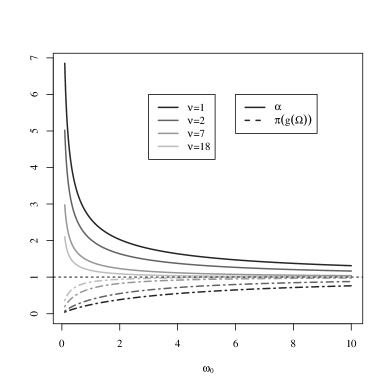
This shows that as the global scale parameter $\omega_{0}$ increases, $\alpha(\omega_{+},\omega_{0},\nu)$ approaches $1$ from above, and $\pi(g_{\omega_{0},\nu}(\boldsymbol{\Omega}))$ approaches $1$ from below. If one interprets $\alpha(\omega_{+},\omega_{0},\nu)$ as governing the worst-case efficiency of $\boldsymbol{\beta}^{*}$ relative to the ordinary least squares estimate and $\pi(g_{\omega_{0},\nu}(\boldsymbol{\Omega}))$ as governing its improvement in efficiency relative to the ordinary least squares estimate, one concludes that higher values of $\omega_{0},\nu$ leave less room for improvement, but also less room to fail. Since $\alpha(\omega_{+},\omega_{0},\nu)$ never falls below $1$, the worst-case asymptotic generalized variance of $\boldsymbol{\beta}^{*}$ cannot be better than that of the ordinary least squares estimate.

The next numerical examples demonstrate that this worst-case view may be too pessimistic in practice. In Figure 3, we compare the variance of several estimates with respect to the model (1) with normal errors and fixed design matrix ${\mathbf{X}}\in\mathbb{R}^{n\times 4}$, which has entries drawn independently from a standard normal distribution. In this example, $n=1000$, and the entries of $\boldsymbol{\Omega}$ are set to the $1/(n+1),\dots,n/(n+1)$ quantiles of an inverse gamma distribution with parameters $\nu/2,\nu/2$. We evaluate the root generalized variance of $\boldsymbol{\beta}^{*}$, which we define to be $|{\mathbf{V}}_{n}^{-1}{\mathbf{B}}_{n}{\mathbf{V}}_{n}^{-1}|^{1/p}$, both for an oracle estimate, where the degrees of freedom are set to the true value of $\nu$

$\displaystyle{\mathbf{V}}_{n}=\sum_{i=1}^{n}\frac{1}{g_{\omega_{0},\nu}(\omega_{i})}{\mathbf{x}}_{i}{\mathbf{x}}_{i}^{\top},~{}{\mathbf{B}}_{n}=\sum_{i=1}^{n}\frac{1}{f_{\omega_{0},\nu}(\omega_{i})}{\mathbf{x}}_{i}{\mathbf{x}}_{i}^{\top},$ (14)

and for an estimate using $7$ degrees of freedom, where

$\displaystyle{\mathbf{V}}_{n}=\sum_{i=1}^{n}\frac{1}{g_{\omega_{0},7}(\omega_{i})}{\mathbf{x}}_{i}{\mathbf{x}}_{i}^{\top},~{}{\mathbf{B}}_{n}=\sum_{i=1}^{n}\frac{1}{f_{\omega_{0},7}(\omega_{i})}{\mathbf{x}}_{i}{\mathbf{x}}_{i}^{\top}.$

We set aside the issue of varying the scale parameter $\omega_{0}$, for now, as we set it equal to $1$ for both estimates. We also evaluate $|H_{{\mathbf{X}}}({\mathbf{I}}_{n},\boldsymbol{\Omega})|^{1/p}$ and $|H_{{\mathbf{X}}}(\boldsymbol{\Omega},\boldsymbol{\Omega})|^{1/p}$, corresponding to the root generalized variance of the ordinary and weighted least squares estimates, respectively.

Refer to caption
Figure 3: Theoretical behavior of $t$-derived estimates. On the left, a comparison of the root generalized variance of three estimates relative to that of the weighted least squares estimate for small degrees of freedom. On the right, the same comparison is made for large degrees of freedom.

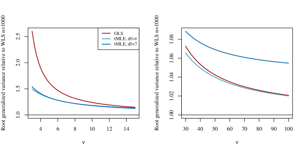
The left panel of Figure 3 plots the root generalized variance of each estimate divided by that of the weighted least squares estimate for values of $\nu$ ranging from $3$ to $15$. The right panel zooms in on the relative root generalized variances for the range $\nu=30$ to $\nu=100$. For all values of $\nu$ between $3$ and $15$, the oracle $\boldsymbol{\beta}^{*}$ has lower root generalized variance than the ordinary least squares estimate. This is also true of the root generalized variance of the non-oracle estimate using the fixed value of $7$ degrees of freedom, and it is interesting to note that these two versions of $\boldsymbol{\beta}^{*}$ behave similarly in this range. For values of $\nu$ between $30$ and $100$, the ordinary least squares estimate outperforms the non-oracle $\boldsymbol{\beta}^{*}$, though the difference between them is quite small. To summarize, maximum likelihood estimates derived from linear models with independent $t$ errors can be substantially more efficient than the ordinary least squares estimate if the dispersion among the elements of $\boldsymbol{\Omega}$ is moderate to high. When the dispersion is low, and $\boldsymbol{\Omega}$ is close to ${\mathbf{I}}_{n}$, ordinary least squares performs better than a non-oracle $t$-derived maximum likelihood estimate, but only by a small amount.

While useful for the purposes of illustration, the previous example is somewhat artificial in terms of the choice of ${\mathbf{X}}$ and $\boldsymbol{\Omega}$. It also relies only on formulae like those in (14) to calculate the variance of various estimates. The next numerical example features a data-derived design matrix and approximate root generalized variances computed using Monte Carlo in addition to those computed using the values of $\boldsymbol{\Omega}$ as input. This allows us to compare the theoretical behavior of $t$-derived estimates to their behavior in practice.

Several ground-truth quantities need to be defined for this simulation. First, the design matrix ${\mathbf{X}}$ is chosen to be a $2370\times 17$ matrix, corresponding to a subset of the data collected during a study of the association between the concentration of pesticide byproducts in maternal serum and preterm births (Longnecker et al., 2001). Each row of ${\mathbf{X}}$ corresponds to a birth occurring between 1959 and 1966. In addition to an intercept term, the columns of ${\mathbf{X}}$ are comprised of maternal serum concentrations of 12 environmental contaminants, as well as maternal triglyceride level, age, smoking status, and cholesterol. We scale all non-intercept columns of ${\mathbf{X}}$ to have variance equal to $1$.

Next, we set ground truth parameters $\nu,\omega_{0},\boldsymbol{\beta}$ equal to the maximum marginal likelihood estimates of the parameters in the independent $t$ model (12), where the dependent variable ${\mathbf{y}}$ is the gestational age—also recorded as part of the Longnecker et al. (2001) study—of each of the births in ${\mathbf{X}}$. These parameters are computed using an EM-algorithm, which we describe in the appendix (see also Lange and Sinsheimer (1993); Liu and Rubin (1995)). Finally, the error covariance matrix $\boldsymbol{\Omega}$ is set equal to a $2370\times 2370$ diagonal matrix, whose diagonal entries are independent draws from an inverse gamma distribution with parameters $\nu/2,\nu\omega_{0}/2$. In preparation for the simulation study, we also preallocate the submatrices ${\mathbf{X}}_{1:n}$ consisting of the first $n$ rows of ${\mathbf{X}}$ for $n\in\{50,100,200,500,1000,2370\}$. Similarly, we form the error covariance matrices $\boldsymbol{\Omega}_{1:n,1:n}$ consisting of the first $n$ rows and columns of $\boldsymbol{\Omega}$.

Using these quantities as our ground-truth, we evaluate the root generalized variance of five estimates of $\boldsymbol{\beta}$ with respect to the heteroscedastic normal linear model (1). The estimates are: the ordinary least squares estimate, the $t$ maximum likelihood estimate with estimated scale parameter and estimated degrees of freedom, the $t$ maximum likelihood estimate with estimated scale parameter and $7$ degrees of freedom, the “oracle” $t$ maximum likelihood estimate with scale parameter and degrees of freedom equal to the ground-truth $\omega_{0},\nu$, and the weighted least squares estimate. For each $n$, the root generalized variance of the non-oracle $t$-derived estimates are computed using Monte Carlo; that is, we simulate $1000$ instances of ${\mathbf{y}}\in\mathbb{R}^{n}$ according to (1), compute a $\boldsymbol{\beta}^{*}$ for each instance in order to form an $1000\times 17$ matrix of estimates, compute the sample covariance matrix of the estimates, and then take the geometric mean of the eigenvalues of this matrix. For the ordinary and weighted least squares estimates, we use the formulae $|H_{{\mathbf{X}}_{1:n}}({\mathbf{I}}_{n},\boldsymbol{\Omega}_{1:n,1:n})|^{1/17}$ and $|H_{{\mathbf{X}}_{1:n}}(\boldsymbol{\Omega}_{1:n,1:n},\boldsymbol{\Omega}_{1:n,1:n})|^{1/17}$, respectively. For the oracle $t$ estimate, we use $|{\mathbf{V}}_{n}^{-1}{\mathbf{B}}_{n}{\mathbf{V}}_{n}^{-1}|^{1/17}$ with ${\mathbf{V}}_{n},{\mathbf{B}}_{n}$ defined as in (14)italic-(14italic-)\eqref{eq:oracle}.

Refer to caption
Figure 4: Results of the first simulation study using the Longnecker et al. (2001) dataset, which uses a sample of inverse gamma distributed random variables to specify the heteroscedasticity.

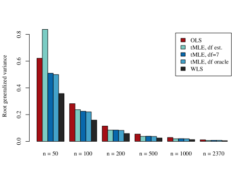
Figure 4 displays the root generalized variance for each of the estimates described above. When interpreting these results, it should be kept in mind that only the ordinary least squares estimate and the two non-oracle $t$-derived estimates can be computed in practice. Of these latter two, only the $t$ estimate with fixed degrees of freedom outperforms the ordinary least squares estimate for each value of $n$. For $n\geq 200$, though, the $t$-derived estimate with estimated degrees of freedom slightly outperforms the estimate with fixed degrees of freedom. This result is consistent with the results shown in Figure 3. We also note that the behavior of both non-oracle $t$ estimates closely matches that of the oracle $t$ estimate for $n\geq 200$, which provides some assurance that the asymptotic formulae derived in Theorem 2 hold, and that the rate of convergence to this limit is not too slow.

Next, we conduct a simulation similar to the one above using a different specification of heteroscedasticity. Specifically, we set

$$\omega_{i}=1.1|x_{i,15}|^{3}|x_{i,16}|^{2},~{}i=1,\dots,n,$$

which is a particular instance of the flexible parametric model of heteroscedasticity

$$v_{\boldsymbol{\theta}}({\mathbf{x}}_{i})=e^{\theta_{1}}\prod_{j=2}^{p}|x_{i,j}|^{\theta_{j}}$$

suggested by Romano and Wolf (2017). Columns 15 and 16 of ${\mathbf{X}}$ correspond to maternal age and smoking status, respectively, and, as before, the first column of ${\mathbf{X}}$ is ${\mathbf{1}}_{n}/\sqrt{n}$. All other aspects of this simulation are then the same as above, except we substitute a parametric feasible weighted least squares estimate for the oracle $t$ estimate. The parametric feasible weighted least squares estimate takes the form $b_{{\mathbf{X}}_{1:n}}(\hat{\boldsymbol{\Omega}}_{n})$ for

$$\hat{\boldsymbol{\Omega}}_{n}=\mathrm{diag}(v_{\hat{\boldsymbol{\theta}}_{n}}({\mathbf{x}}_{1}),\dots,v_{\hat{\boldsymbol{\theta}}_{n}}({\mathbf{x}}_{n})),$$

where $\hat{\boldsymbol{\theta}}_{n}$ is the ordinary least squares solution to the regression implied by

$$\log\{\max(0.01^{2},\hat{\varepsilon}_{i}^{2})\}=\theta_{1}+\sum_{j=2}^{17}\theta_{j}\log|x_{i,j}|+z_{i},~{}z_{i}\sim N(0,1),~{}i=1,\dots,n,$$

and $\hat{\varepsilon}_{i}$ is the $i$th residual from the ordinary least squares fit of $\boldsymbol{\beta}$. We evaluate the root generalized variance of $b_{{\mathbf{X}}_{1:n}}(\hat{\boldsymbol{\Omega}}_{n})$ using Monte Carlo and display it along with the root generalized variance of the other estimates in Figure 5.

Refer to caption
Figure 5: Results of the second simulation study using the Longnecker et al. (2001) dataset, which uses a parametric model to specify the heteroscedasticity.

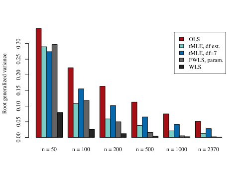
Here we see that the root generalized variance of both $t$-derived estimates is less than that of the ordinary least squares estimate for $n\geq 100$. Notably, the $t$ estimate with fixed $\nu=7$ performs worse with respect to the $t$ estimate with estimated $\nu$ relative to the previous simulation for $n\geq 100$. Perhaps more strikingly, these results suggest that the $t$-derived estimate with estimated degrees of freedom performs quite favorably relative to the feasible weighted least squares estimate for $n\leq 200$, and this is when the parametric form of heteroscedasticity is correctly specified. Of course, when $n$ is large, the correctly specified parametric feasible weighted least squares estimate is nearly optimal, while the $t$-derived estimates lag behind.

6 Discussion

The experiments of the previous section suggest that $t$-derived estimates can be substantially more efficient than the ordinary least squares estimate in the heteroscedastic linear model with normally distributed errors. The theoretical results in this article suggest that this improvement in efficiency can be attributed to a quasi-oracle property of the $t$-derived estimates: in the limit, these estimates are sub-optimal, but are still preferable to ordinary least squares because they are nearly equivalent to a feasible weighted least squares estimate using compromise weights. From the perspective of point estimation in the heteroscedastic linear model, we contend that there is little downside to using $t$-derived estimates, especially those with fixed degrees of freedom, in place of the ordinary least squares estimate.

A complete case for abandoning the ordinary least squares estimate in favor of the $t$ maximum likelihood estimate should include tools for inference in addition to those for point estimation. While we did not discuss the construction of confidence intervals for $\boldsymbol{\beta}$ in this article, we believe that the main theorems from Hoadley (1971) and White (1980b, a) can be used to derive consistent standard errors for the $t$-derived estimates. These may then be used to obtain confidence intervals with the correct asymptotic coverage probability.

In future theoretical work, the perspective of compromise sets may also be applied to linear models with non-diagonal error covariance. Indeed, if $\tilde{\boldsymbol{\Omega}}$ and $\boldsymbol{\Omega}$ are simultaneously diagonalizable, then Corollary 1 may be applied directly to this case, substituting the eigenvalues of $\tilde{\boldsymbol{\Omega}}$ and $\boldsymbol{\Omega}$ for their diagonal entries. Compromise sets may also be a lens through which to analyze regression $M$-estimates other than those derived from the $t$-distribution. For instance, the second function in Figure 1, which obeys the growth-restricted monotonicity property of Proposition 1, arises when deriving the asymptotic variance of the Huber estimate (Huber, 1964) (see also Appendix C). Hence, it is possible that compromise sets provide an explanation for the robustness properties of a whole class of $M$-estimates in the presence of heteroscedasticity.

References

  • Aitken (1936) Aitken, A. C. (1936). IV.—On Least Squares and Linear Combination of Observations. Proc. R. Soc. Edinb. 55, 42–48.
  • Anderson (1948) Anderson, T. (1948, July). On the theory of testing serial correlation. Scandinavian Actuarial Journal 1948(3-4), 88–116.
  • Atkinson et al. (2016) Atkinson, A. C., M. Riani, and F. Torti (2016, December). Robust methods for heteroskedastic regression. Computational Statistics & Data Analysis 104, 209–222.
  • Bilodeau (1990) Bilodeau, M. (1990, January). On the choice of loss function in covariance estimation. Statistics & Risk Modeling 8(2).
  • Bloomfield and Watson (1975) Bloomfield, P. and G. S. Watson (1975). The inefficiency of least squares. Biometrika 62(1), 121–128.
  • Bryan and Hoff (2023) Bryan, J. and P. Hoff (2023). Linear Source Apportionment using Generalized Least Squares. Publisher: [object Object] Version Number: 1.
  • Bryan et al. (2023) Bryan, J., P. Hoff, and C. L. Osburn (2023, August). Routine Estimation of Dissolved Organic Matter Sources Using Fluorescence Data and Linear Least Squares. ACS EST Water 3(8), 2073–2082.
  • Hoadley (1971) Hoadley, B. (1971, December). Asymptotic Properties of Maximum Likelihood Estimators for the Independent Not Identically Distributed Case. Ann. Math. Statist. 42(6), 1977–1991.
  • Huber (1964) Huber, P. J. (1964, March). Robust Estimation of a Location Parameter. Ann. Math. Statist. 35(1), 73–101.
  • Huber (1973) Huber, P. J. (1973, September). Robust Regression: Asymptotics, Conjectures and Monte Carlo. Ann. Statist. 1(5).
  • Huber and Ronchetti (2009) Huber, P. J. and E. M. Ronchetti (2009, January). Robust Statistics (1 ed.). Wiley Series in Probability and Statistics. Wiley.
  • Johnson et al. (1994) Johnson, N. L., S. Kotz, and N. Balakrishnan (1994). Continuous univariate distributions (2nd ed ed.). Wiley series in probability and mathematical statistics. New York: Wiley.
  • Kariya and Kurata (2004) Kariya, T. and H. Kurata (2004). Generalized least squares. Wiley series in probability and statistics. Chichester: Wiley.
  • Khatri and Rao (1981) Khatri, C. and C. Rao (1981, December). Some extensions of the Kantorovich inequality and statistical applications. Journal of Multivariate Analysis 11(4), 498–505.
  • Knott (1975) Knott, M. (1975). On the minimum efficiency of least squares. Biometrika 62(1), 129–132.
  • Kurata and Kariya (1996) Kurata, H. and T. Kariya (1996, August). Least upper bound for the covariance matrix of a generalized least squares estimator in regression with applications to a seemingly unrelated regression model and a heteroscedastic model. Ann. Statist. 24(4).
  • Lange and Sinsheimer (1993) Lange, K. and J. S. Sinsheimer (1993, June). Normal/Independent Distributions and Their Applications in Robust Regression. Journal of Computational and Graphical Statistics 2(2), 175.
  • Lange et al. (1989) Lange, K. L., R. J. A. Little, and J. M. G. Taylor (1989, December). Robust Statistical Modeling Using the t Distribution. Journal of the American Statistical Association 84(408), 881.
  • Ledoit and Wolf (2004) Ledoit, O. and M. Wolf (2004, February). A well-conditioned estimator for large-dimensional covariance matrices. Journal of Multivariate Analysis 88(2), 365–411.
  • Liu and Rubin (1995) Liu, C. and D. B. Rubin (1995, January). ML estimation of the t distribution using EM and its extensions, ECM and ECME. Statistica Sinica 5.
  • Longnecker et al. (2001) Longnecker, M. P., M. A. Klebanoff, H. Zhou, and J. W. Brock (2001, July). Association between maternal serum concentration of the DDT metabolite DDE and preterm and small-for-gestational-age babies at birth. The Lancet 358(9276), 110–114.
  • Maronna (1976) Maronna, R. A. (1976, January). Robust $M$-Estimators of Multivariate Location and Scatter. Ann. Statist. 4(1).
  • Marshall and Olkin (1990) Marshall, A. W. and I. Olkin (1990, December). Matrix versions of the Cauchy and Kantorovich inequalities. Aeq. Math. 40(1), 89–93.
  • Marshall et al. (2011) Marshall, A. W., I. Olkin, and B. C. Arnold (2011). Inequalities: Theory of Majorization and Its Applications. Springer Series in Statistics. New York, NY: Springer New York.
  • Perić et al. (2019) Perić, Z. H., J. R. Nikolić, and M. D. Petković (2019, April). Class of tight bounds on the Q ‐function with closed‐form upper bound on relative error. Math Methods in App Sciences 42(6), 1786–1794.
  • Romano and Wolf (2017) Romano, J. P. and M. Wolf (2017, March). Resurrecting weighted least squares. Journal of Econometrics 197(1), 1–19.
  • Romanov et al. (2023) Romanov, E., G. Kur, and B. Nadler (2023, July). Tyler’s and Maronna’s M-estimators: Non-asymptotic concentration results. Journal of Multivariate Analysis 196, 105184.
  • Schmidt (2014) Schmidt, K. D. (2014, March). On inequalities for moments and the covariance of monotone functions. Insurance: Mathematics and Economics 55, 91–95.
  • Shah et al. (2023) Shah, K. S., H. Fu, and M. R. Kosorok (2023, January). Stabilized direct learning for efficient estimation of individualized treatment rules. Biometrics, biom.13818.
  • Stefanski and Boos (2002) Stefanski, L. A. and D. D. Boos (2002, February). The Calculus of M-Estimation. The American Statistician 56(1), 29–38.
  • Wang and Yang (1989) Wang, S. and H. Yang (1989, December). Kantorovich-type inequalities and the measures of inefficiency of the glse. Acta Mathematicae Applicatae Sinica 5(4), 372–381.
  • Watson (1967) Watson, G. S. (1967, December). Linear Least Squares Regression. Ann. Math. Statist. 38(6), 1679–1699.
  • Watson (1972) Watson, G. S. (1972, April). Prediction and the efficiency of least squares. Biometrika 59(1), 91–98.
  • White (1980a) White, H. (1980a, May). A Heteroskedasticity-Consistent Covariance Matrix Estimator and a Direct Test for Heteroskedasticity. Econometrica 48(4), 817.
  • White (1980b) White, H. (1980b, April). Nonlinear Regression on Cross-Section Data. Econometrica 48(3), 721.
  • Wooldridge (2010) Wooldridge, J. M. (2010). Econometric analysis of cross section and panel data. MIT press.
  • Wooldridge et al. (2016) Wooldridge, J. M., M. Wadud, and J. Lye (2016). Introductory econometrics: Asia pacific edition with online study tools 12 months. Cengage AU.

Appendix A Proofs

A.1 Proof of Proposition 1

Proof.

Let $p=1$, and for each $i\in\{1,\dots,n\}$, let $\tilde{\omega}_{i}=g(\omega_{i})$ where $g$ is a monotone non-decreasing function such that the function $f(\omega)=g(\omega)/\omega$ is monotone non-increasing. Set $\tilde{\boldsymbol{\Phi}}=\tilde{\boldsymbol{\Omega}}^{-1}$, and let $\mathcal{V}^{n}$ denote the set of all $n$-dimensional unit vectors.

As discussed in the main text, for any unit vector ${\mathbf{u}}$ the functions $\mathrm{e}_{{\mathbf{u}}}$ and $\mathrm{c}_{{\mathbf{u}}}$ behave, respectively, like the expectation and covariance functions of discrete random variables with supports determined by the diagonal entries of $\tilde{\boldsymbol{\Omega}},\boldsymbol{\Omega}$ and probability mass functions determined by ${\mathbf{u}}$. Therefore, by Schmidt (2014) Corollary 3.1,

$$\mathrm{c}_{{\mathbf{u}}}(\tilde{\boldsymbol{\Phi}},\boldsymbol{\Omega})\leq 0,~{}\forall{\mathbf{u}}\in\mathcal{V}^{n},$$

and

$$\mathrm{c}_{{\mathbf{u}}}(\tilde{\boldsymbol{\Phi}},\tilde{\boldsymbol{\Phi}}\boldsymbol{\Omega})\leq 0,~{}\forall{\mathbf{u}}\in\mathcal{V}^{n}.$$

Thus,

$$\mathrm{c}_{{\mathbf{u}}}(\tilde{\boldsymbol{\Phi}},\tilde{\boldsymbol{\Phi}}\boldsymbol{\Omega})+\mathrm{e}_{{\mathbf{u}}}(\tilde{\boldsymbol{\Phi}})\mathrm{c}_{{\mathbf{u}}}(\tilde{\boldsymbol{\Phi}},\boldsymbol{\Omega})\leq 0,~{}\forall{\mathbf{u}}\in\mathcal{V}^{n},$$

so $\tilde{\boldsymbol{\Omega}}\in\mathcal{C}^{1}_{\boldsymbol{\Omega}}$. ∎

A.2 Proof of Theorem 1

To prove Theorem 1, we first present the following lemma:

Lemma 1.

Let $\tilde{\boldsymbol{\Phi}},\boldsymbol{\Omega}\in\mathcal{D}_{+}^{n}$. Let $\mathcal{V}^{n}$ denote the set of all $n$-dimensional unit vectors. Define the function $k:\mathbb{R}^{n}\rightarrow\mathbb{R}$ by

$$k({\mathbf{u}})={\mathbf{u}}^{\top}\tilde{\boldsymbol{\Phi}}\boldsymbol{\Omega}\tilde{\boldsymbol{\Phi}}{\mathbf{u}}-({\mathbf{u}}^{\top}\tilde{\boldsymbol{\Phi}}{\mathbf{u}})^{2}({\mathbf{u}}^{\top}\boldsymbol{\Omega}{\mathbf{u}}).$$

Then

$$\sup_{{\mathbf{u}}\in\mathcal{V}^{n}}~{}k({\mathbf{u}})=\sup_{{\mathbf{u}}\in\mathcal{V}^{n},\|{\mathbf{u}}\|_{0}\leq 2}~{}k({\mathbf{u}}).$$
Proof.

We will prove the statement by providing, for any ${\mathbf{u}}\in\mathcal{V}^{n}$, a corresponding ${\mathbf{v}}\in\mathcal{V}^{n}$ with $\|{\mathbf{v}}\|_{0}\leq 2$ such that

$$k({\mathbf{u}})\leq k({\mathbf{v}}).$$

Given $\tilde{\boldsymbol{\Phi}},\boldsymbol{\Omega}\in\mathcal{D}_{+}^{n}$, let ${\mathbf{u}}\in\mathcal{V}^{n}$ and let $\boldsymbol{\alpha}={\mathbf{u}}\odot{\mathbf{u}}$, where $\odot$ denotes the Hadamard product. Further, let $\boldsymbol{\alpha}^{1/2}$ denote the entrywise positive square root of $\boldsymbol{\alpha}$ so that $(\boldsymbol{\alpha}^{1/2})_{i}=|u_{i}|$ for each $i\in\{1,\dots,n\}$. Note that in terms of $\boldsymbol{\alpha}$, $k({\mathbf{u}})$ may be written as

$$\boldsymbol{\alpha}^{\top}(\tilde{\boldsymbol{\phi}}\odot\tilde{\boldsymbol{\phi}}\odot\boldsymbol{\omega})-(\boldsymbol{\alpha}^{\top}\tilde{\boldsymbol{\phi}})^{2}(\boldsymbol{\alpha}^{\top}\boldsymbol{\omega}),$$ (15)

where $\tilde{\phi},\boldsymbol{\omega}$ are $n$-dimensional vectors containing the diagonal elements of $\tilde{\boldsymbol{\Phi}},\boldsymbol{\Omega}$, respectively.

If $\|{\mathbf{u}}\|_{0}\leq 2$, then setting ${\mathbf{v}}:={\mathbf{u}}$ yields a trivial bound satisfying the norm constraint. Suppose instead that $\|{\mathbf{u}}\|_{0}=d>4$, and let $\mathcal{I}_{{\mathbf{u}}}$ be the index set of the non-zero entries of ${\mathbf{u}}$. Then there exists a vector $\boldsymbol{\eta}\in\mathbb{R}^{n}$ such that

$$\boldsymbol{\eta}^{\top}(\tilde{\boldsymbol{\phi}}\odot\tilde{\boldsymbol{\phi}}\odot\boldsymbol{\omega})=0,~{}\boldsymbol{\eta}^{\top}\boldsymbol{\omega}=0,~{}\boldsymbol{\eta}^{\top}\tilde{\boldsymbol{\phi}}=0,~{}\boldsymbol{\eta}^{\top}{\mathbf{1}}_{n}=0$$ (16)

and $\eta_{i}=0$ for $i\notin\mathcal{I}_{{\mathbf{u}}}$. Such an $\boldsymbol{\eta}$ exists because these restrictions define a system of at most $n-1$ independent linear equations in $n$ variables. To see this, note that there are four linear equations in (16), and there are $n-d$ linear equations that enforce $\eta_{i}=0$ for $i\notin\mathcal{I}_{{\mathbf{u}}}$. As $d>4$, the number of linear equations is $n-d+4<n$. If $\boldsymbol{\omega},\tilde{\boldsymbol{\phi}}$ and ${\mathbf{1}}_{n}$ are linearly independent, then the number of independent linear equations is exactly $n-d+4$. If they are not, then the effective number of independent linear equations is less than $n-d+4$.

An $\boldsymbol{\eta}$ satisfying the restrictions above must also have at least one negative entry and one positive entry among its non-zero entries. This is due to the fact that $\boldsymbol{\omega},\tilde{\boldsymbol{\phi}}$ and ${\mathbf{1}}_{n}$ are all vectors with strictly positive entries, so (16) implies that $\boldsymbol{\eta}$ cannot lie in either the positive orthant or the negative orthant. Consequently, there exists an $\epsilon>0$ such that $\|\boldsymbol{\alpha}+\epsilon\boldsymbol{\eta}\|_{0}=d-1$ and the entries of $\boldsymbol{\alpha}+\epsilon\boldsymbol{\eta}$ are all non-negative. Specifically, if

$$\epsilon=\min_{\{i:\eta_{i}<0\}}|\alpha_{i}/\eta_{i}|,$$

then no entry of $\boldsymbol{\alpha}+\epsilon\boldsymbol{\eta}$ will fall below zero, and $\boldsymbol{\alpha}+\epsilon\boldsymbol{\eta}$ will have one additional entry equal to zero (the entry corresponding to the minimum above) relative to $\boldsymbol{\alpha}$.

Setting ${\mathbf{v}}:=(\boldsymbol{\alpha}+\epsilon\boldsymbol{\eta})^{1/2}$ produces a unit vector with $L_{0}$ norm equal to $d-1$ such that $k({\mathbf{u}})=k({\mathbf{v}})$. The fact that ${\mathbf{v}}$ is a unit vector follows from

$\displaystyle{\mathbf{v}}^{\top}{\mathbf{v}}$ $\displaystyle=\sum_{i=1}^{n}|\alpha_{i}+\epsilon\eta_{i}|$
$\displaystyle=\sum_{i=1}^{n}(\alpha_{i}+\epsilon\eta_{i})$
$\displaystyle={\mathbf{1}}^{\top}\boldsymbol{\alpha}+\epsilon{\mathbf{1}}^{\top}\boldsymbol{\eta}$
$\displaystyle=1,$

where we used the last linear equation in (16) to obtain the last equality. The fact that ${\mathbf{v}}$ has $L_{0}$ norm equal to $d-1$ follows from the fact that $\|\boldsymbol{\alpha}+\epsilon\boldsymbol{\eta}\|_{0}=d-1$. Finally, $k({\mathbf{u}})=k({\mathbf{v}})$ because the first three linear equations in (16) ensure that none of the terms in (15) change when $\boldsymbol{\alpha}+\epsilon\boldsymbol{\eta}$ is substituted for $\boldsymbol{\alpha}$. Each of the steps above can be repeated until one begins the process with $d=5$ and obtains a valid ${\mathbf{v}}$ with $L_{0}$ norm equal to $4$. This demonstrates that

$$\sup_{{\mathbf{u}}\in\mathcal{V}^{n}}~{}k({\mathbf{u}})=\sup_{{\mathbf{u}}\in\mathcal{V}^{n},\|{\mathbf{u}}\|_{0}\leq 4}~{}k({\mathbf{u}}).$$

It remains to address the case that $2<\|{\mathbf{u}}\|_{0}\leq 4$.

If $\|{\mathbf{u}}\|_{0}=4$, then there exists a non-zero vector $\boldsymbol{\eta}\in\mathbb{R}^{n}$ such that

$$\boldsymbol{\eta}^{\top}(\tilde{\boldsymbol{\phi}}\odot\tilde{\boldsymbol{\phi}}\odot\boldsymbol{\omega})>0,~{}\boldsymbol{\eta}^{\top}\boldsymbol{\omega}=0,~{}\boldsymbol{\eta}^{\top}\tilde{\boldsymbol{\phi}}=0,~{}\boldsymbol{\eta}^{\top}{\mathbf{1}}_{n}=0$$ (17)

and $\eta_{i}=0$ for each $i\notin\mathcal{I}_{{\mathbf{u}}}$. Reasoning as before, such an $\boldsymbol{\eta}$ exists because there is at least a $1$-dimensional subspace of $\mathbb{R}^{n}$ where the stated equalities are satisfied. If we choose an arbitrary vector in this subspace, it will either have positive or negative dot product with $(\tilde{\boldsymbol{\phi}}\odot\tilde{\boldsymbol{\phi}}\odot\boldsymbol{\omega})$. If the dot product is positive, we can choose $\boldsymbol{\eta}$ to be this vector. If it is negative then we can choose $\boldsymbol{\eta}$ to be the negation of this vector. Having found such an $\boldsymbol{\eta}$, we may again choose

$$\epsilon=\min_{\{i:\eta_{i}<0\}}|\alpha_{i}/\eta_{i}|,$$

and note, as before, that $(\boldsymbol{\alpha}+\epsilon\boldsymbol{\eta})^{1/2}$ is a unit vector with three non-zero, positive entries. Here, setting ${\mathbf{v}}:=(\boldsymbol{\alpha}+\epsilon\boldsymbol{\eta})^{1/2}$ yields $k({\mathbf{u}})<k({\mathbf{v}})$ due to the inequality in (17). This implies that it suffices to consider the $\|{\mathbf{u}}\|_{0}=3$ case.

If $\|{\mathbf{u}}\|_{0}=3$, then there exists a non-zero vector $\boldsymbol{\eta}\in\mathbb{R}^{n}$ such that

$$\boldsymbol{\eta}^{\top}\left\{(\tilde{\boldsymbol{\phi}}\odot\tilde{\boldsymbol{\phi}}\odot\boldsymbol{\omega})-(\boldsymbol{\alpha}^{\top}\tilde{\boldsymbol{\phi}})^{2}\boldsymbol{\omega}\right\}>0,~{}\boldsymbol{\eta}^{\top}\tilde{\boldsymbol{\phi}}=0,~{}\boldsymbol{\eta}^{\top}{\mathbf{1}}_{n}=0$$ (18)

and $\eta_{i}=0$ for each $i\notin\mathcal{I}_{{\mathbf{u}}}$. Such an $\boldsymbol{\eta}$ exists because there is at least a $1$-dimensional subspace of $\mathbb{R}^{n}$ where the stated equalities are satisfied. If we choose an arbitrary vector in this subspace, it will either have positive or negative dot product with the vector $(\tilde{\boldsymbol{\phi}}\odot\tilde{\boldsymbol{\phi}}\odot\boldsymbol{\omega})-(\boldsymbol{\alpha}^{\top}\tilde{\boldsymbol{\phi}})^{2}\boldsymbol{\omega}$. If the dot product is positive, we can choose $\boldsymbol{\eta}$ to be this vector. If it is negative then we can choose $\boldsymbol{\eta}$ to be the negation of this vector. Having found such an $\boldsymbol{\eta}$, we may again choose

$$\epsilon=\min_{\{i:\eta_{i}<0\}}|\alpha_{i}/\eta_{i}|,$$

and note as before that $(\boldsymbol{\alpha}+\epsilon\boldsymbol{\eta})^{1/2}$ is a unit vector with two non-zero, positive entries. Setting ${\mathbf{v}}:=(\boldsymbol{\alpha}+\epsilon\boldsymbol{\eta})^{1/2}$ yields $k({\mathbf{u}})<k({\mathbf{v}})$ due to the inequality in (18).

Hence, for any ${\mathbf{u}}\in\mathcal{V}^{n}$ there exists a ${\mathbf{v}}\in\mathcal{V}^{n}$ such that $\|{\mathbf{v}}\|_{0}\leq 2$ and $k({\mathbf{u}})<k({\mathbf{v}})$, so

$$\sup_{{\mathbf{u}}\in\mathcal{V}^{n}}~{}k({\mathbf{u}})=\sup_{{\mathbf{u}}\in\mathcal{V}^{n},\|{\mathbf{u}}\|_{0}\leq 2}~{}k({\mathbf{u}}),$$

which completes the proof. ∎

Now we prove Theorem 1:

Proof of Theorem 1.

For the entirety of the proof we assume that the diagonal entries of $\boldsymbol{\Omega},\tilde{\boldsymbol{\Omega}}\in\mathcal{D}_{+}^{n}$ are distinct. The result may be generalized by a continuity argument to the case of non-distinct diagonal entries.

($\impliedby$) We will prove the necessity of (9) by proving that if it does not hold for some $\tilde{\boldsymbol{\Omega}}$, then $\tilde{\boldsymbol{\Omega}}\notin\mathcal{C}^{1}_{\boldsymbol{\Omega}}$. Suppose that the diagonal entries of $\tilde{\boldsymbol{\Omega}}$ do not satisfy

$$1\leq\frac{\tilde{\omega}_{i}}{\tilde{\omega}_{j}}\leq 2\frac{\omega_{i}}{\omega_{j}}-1$$

for all $\omega_{i}>\omega_{j}$, $i\in\{1,\dots,n\},j\in\{1,\dots,n\}$. Then there exists at least one pair of indices, $(i,j)$, for which $\omega_{i}>\omega_{j}$, and either

$$\frac{\tilde{\omega}_{i}}{\tilde{\omega}_{j}}>2\frac{\omega_{i}}{\omega_{j}}-1$$ (19)

or

$$\frac{\tilde{\omega}_{i}}{\tilde{\omega}_{j}}<1.$$ (20)

First, suppose that (19) holds for a pair of indices $(i,j)$, and let ${\mathbf{u}}$ be a unit vector with entries equal to zero everywhere except at the indices $i$ and $j$. Then we may write $t:=u_{i}^{2}$ and $1-t:=u_{j}^{2}$, and after expanding and collecting terms, find that

$\displaystyle\mathrm{c}_{{\mathbf{u}}}(\tilde{\boldsymbol{\Phi}},\tilde{\boldsymbol{\Phi}}\boldsymbol{\Omega})+\mathrm{e}_{{\mathbf{u}}}(\tilde{\boldsymbol{\Phi}})\mathrm{c}_{{\mathbf{u}}}(\tilde{\boldsymbol{\Phi}},\boldsymbol{\Omega})$ $\displaystyle=t(1-t)(\tilde{\phi}_{i}-\tilde{\phi}_{j})^{2}(\omega_{i}-\omega_{j})\left[t-\frac{2\tilde{\phi}_{j}\omega_{j}-(\tilde{\phi}_{i}+\tilde{\phi}_{j})\omega_{i}}{(\tilde{\phi}_{i}-\tilde{\phi}_{j})(\omega_{i}-\omega_{j})}\right],$

where $\tilde{\boldsymbol{\Phi}}=\tilde{\boldsymbol{\Omega}}^{-1}$. This is a third-degree polynomial in $t$, with roots at $r_{1}=0$, $r_{2}=1$, and

$$r_{3}=\frac{2\tilde{\phi}_{j}\omega_{j}-(\tilde{\phi}_{i}+\tilde{\phi}_{j})\omega_{i}}{(\tilde{\phi}_{i}-\tilde{\phi}_{j})(\omega_{i}-\omega_{j})},$$ (21)

respectively. Since we assumed (19), it holds that $\tilde{\phi}_{j}>\tilde{\phi}_{i}$. Therefore, the denominator above is negative, and the sign of $r_{3}$ depends on whether the numerator above is positive or negative.

Supposing first that the numerator is negative implies that $r_{3}$ must be positive. Additionally, $r_{3}$ must be strictly less than 1 because (19) implies

$$2\tilde{\phi}_{i}\omega_{i}<(\tilde{\phi}_{i}+\tilde{\phi}_{j})\omega_{j}.$$

Subtracting $\tilde{\phi}_{i}\omega_{i}+2\tilde{\phi}_{j}\omega_{j}$ from both sides, and adding $\tilde{\phi}_{j}\omega_{i}$ to both sides yields

$$\tilde{\phi}_{i}\omega_{i}+\tilde{\phi}_{j}\omega_{i}-2\tilde{\phi}_{j}\omega_{j}<\tilde{\phi}_{j}\omega_{i}-\tilde{\phi}_{i}\omega_{i}-\tilde{\phi}_{j}\omega_{j}+\tilde{\phi}_{i}\omega_{j},$$

which implies that

$$(\tilde{\phi}_{i}+\tilde{\phi}_{j})\omega_{i}-2\tilde{\phi}_{j}\omega_{j}<(\tilde{\phi}_{j}-\tilde{\phi}_{i})(\omega_{i}-\omega_{j}),$$

so $0<r_{3}<1$. Since there are then three real roots of the cubic equation in the interval $t\in[0,1]$, we conclude that there exists a $t\in(0,1)$ so that the cubic takes on a positive value. Therefore, there exists a ${\mathbf{u}}$ such that $H_{{\mathbf{u}}}(\tilde{\boldsymbol{\Omega}},\boldsymbol{\Omega})>H_{{\mathbf{u}}}({\mathbf{I}}_{n},\boldsymbol{\Omega})$.

If instead $r_{3}$ is negative, we conclude that the cubic polynomial is positive in the entire interval $(0,1)$. This is because the sign of the leading coefficient of the cubic polynomial is negative, so the polynomial must take on positive values on $(-\infty,r_{3})$, negative values on $(r_{3},0)$, positive values on $(0,1)$, and negative values on $(1,\infty)$. Choosing any $t$ in $(0,1)$, we conclude that there exists a ${\mathbf{u}}$ such that $H_{{\mathbf{u}}}(\tilde{\boldsymbol{\Omega}},\boldsymbol{\Omega})>H_{{\mathbf{u}}}({\mathbf{I}}_{n},\boldsymbol{\Omega})$. Since we came to this conclusion both when $r_{3}$ was assumed positive and when it was assumed negative, (19) implies that there exists a ${\mathbf{u}}$ for which $H_{{\mathbf{u}}}(\tilde{\boldsymbol{\Omega}},\boldsymbol{\Omega})>H_{{\mathbf{u}}}({\mathbf{I}}_{n},\boldsymbol{\Omega})$. Hence (19) implies $\tilde{\boldsymbol{\Omega}}\notin\mathcal{C}_{\boldsymbol{\Omega}}$.

If (20) holds for a pair of indices $(i,j)$, then let ${\mathbf{u}}$ be a unit vector with entries equal to zero everywhere except at the indices $i$ and $j$ and set $t:=u_{i}^{2}$ and $1-t:=u_{j}^{2}$ as before. Here, since (20) implies $\tilde{\phi}_{j}<\tilde{\phi}_{i}$, we see that the denominator in (21) is positive. The numerator, on the other hand, must be negative, since

$$2\tilde{\phi}_{j}\omega_{j}<(\tilde{\phi}_{i}+\tilde{\phi}_{j})\omega_{j}<(\tilde{\phi}_{i}+\tilde{\phi}_{j})\omega_{i}.$$

Hence, when (20) holds, $r_{3}<0$. As before, this leads to the conclusion that the cubic polynomial is positive on the entire interval $(0,1)$, so we may find a ${\mathbf{u}}$ such that $H_{{\mathbf{u}}}(\tilde{\boldsymbol{\Omega}},\boldsymbol{\Omega})>H_{{\mathbf{u}}}({\mathbf{I}}_{n},\boldsymbol{\Omega})$. Hence (20) implies $\tilde{\boldsymbol{\Omega}}\notin\mathcal{C}_{\boldsymbol{\Omega}}$.

($\implies$) Assume that the diagonal entries of $\tilde{\boldsymbol{\Omega}}$ satisfy

$$1\leq\frac{\tilde{\omega}_{i}}{\tilde{\omega}_{j}}\leq 2\frac{\omega_{i}}{\omega_{j}}-1$$

for all $\omega_{i}>\omega_{j}$, $i\in\{1,\dots,n\},j\in\{1,\dots,n\}$. Note that $\tilde{\boldsymbol{\Omega}}\in\mathcal{C}^{1}_{\boldsymbol{\Omega}}$ if and only if

$$\underset{{\mathbf{u}}\in\mathcal{V}^{n}}{\sup}~{}H_{{\mathbf{u}}}(\tilde{\boldsymbol{\Omega}},\boldsymbol{\Omega})-H_{{\mathbf{u}}}(\tilde{\boldsymbol{\Omega}},{\mathbf{I}}_{n})\leq 0.$$

By rearrangement of terms, this can be expressed alternately as

$$\underset{{\mathbf{u}}\in\mathcal{V}^{n}}{\sup}~{}\mathrm{c}_{{\mathbf{u}}}(\tilde{\boldsymbol{\Phi}},\tilde{\boldsymbol{\Phi}}\boldsymbol{\Omega})+\mathrm{e}_{{\mathbf{u}}}(\tilde{\boldsymbol{\Phi}})\mathrm{c}_{{\mathbf{u}}}(\tilde{\boldsymbol{\Phi}},\boldsymbol{\Omega})\leq 0,$$

or as

$$\underset{{\mathbf{u}}\in\mathcal{V}^{n}}{\sup}~{}k({\mathbf{u}})\leq 0,$$ (22)

where $k$ is defined as in Lemma 1, and as before $\tilde{\boldsymbol{\Phi}}=\tilde{\boldsymbol{\Omega}}^{-1}$. Hence, it suffices to show that (22) holds to prove that $\tilde{\boldsymbol{\Omega}}\in\mathcal{C}^{1}_{\boldsymbol{\Omega}}$. Applying Lemma 1, the maxima of $k$ are attained for $\|{\mathbf{u}}\|_{0}\leq 2$. Therefore,

$$\underset{{\mathbf{u}}\in\mathcal{V}^{n}}{\sup}~{}k({\mathbf{u}})=\underset{i\neq j}{\max}~{}\underset{0\leq t\leq 1}{\sup}~{}t(1-t)(\tilde{\phi}_{i}-\tilde{\phi}_{j})^{2}(\omega_{i}-\omega_{j})\left[t-\frac{2\tilde{\phi}_{j}\omega_{j}-(\tilde{\phi}_{i}+\tilde{\phi}_{j})\omega_{i}}{(\tilde{\phi}_{i}-\tilde{\phi}_{j})(\omega_{i}-\omega_{j})}\right]$$ (23)

If the diagonal entries of $\tilde{\boldsymbol{\Omega}}$ satisfy

$$1\leq\frac{\tilde{\omega}_{i}}{\tilde{\omega}_{j}}\leq 2\frac{\omega_{i}}{\omega_{j}}-1$$

for all $\omega_{i}>\omega_{j}$, $i\in\{1,\dots,n\},j\in\{1,\dots,n\}$, then none of the above polynomials can attain a positive value. To see this, re-write the condition above in terms of $\tilde{\phi}_{i},\tilde{\phi}_{j}$ and conclude from the first inequality that $\tilde{\phi}_{i}<\tilde{\phi}_{j}$. From the second inequality, derive

$\displaystyle\frac{\tilde{\phi}_{j}}{\tilde{\phi}_{i}}\leq 2\frac{\omega_{i}}{\omega_{j}}-1$ $\displaystyle\implies\tilde{\phi}_{j}\omega_{j}\leq 2\phi_{i}\omega_{i}-\phi_{i}\omega_{j}$
$\displaystyle\implies\tilde{\phi}_{j}\omega_{i}-\tilde{\phi}_{j}\omega_{j}-\tilde{\phi}_{i}\omega_{i}+\tilde{\phi}_{i}\omega_{j}\leq\tilde{\phi}_{i}\omega_{i}+\tilde{\phi}_{j}\omega_{i}-2\tilde{\phi}_{j}\omega_{j}$
$\displaystyle\implies(\tilde{\phi}_{j}-\tilde{\phi}_{i})(\omega_{i}-\omega_{j})\leq(\tilde{\phi}_{i}+\tilde{\phi}_{j})\omega_{i}-2\tilde{\phi}_{j}\omega_{j}$

Since $\tilde{\phi}_{i}<\tilde{\phi}_{j}$, we conclude that

$$\frac{2\tilde{\phi}_{j}\omega_{j}-(\tilde{\phi}_{i}+\tilde{\phi}_{j})\omega_{i}}{(\tilde{\phi}_{i}-\tilde{\phi}_{j})(\omega_{i}-\omega_{j})}\geq 1,$$

so the third root of all polynomials in (23) is greater than or equal to 1. Denote this root by $r_{3}$ as before, and first assume $r_{3}>1$. In this case, since the leading coefficient in each of the cubic polynomials in (23) is negative, each polynomial must be positive on $(-\infty,0)$, negative on $(0,1)$, positive on $(1,r_{3})$, and negative on $(r_{3},\infty)$. If $r_{3}=1$, then there is a repeated root at $1$, and the polynomial is non-positive on $(0,\infty)$. Thus, all polynomials in (23) are non-positive on the interval $[0,1]$. ∎

A.3 Proof of Corollary 1

Proof.

For the entirety of the proof we assume that the diagonal entries of $\boldsymbol{\Omega},\tilde{\boldsymbol{\Omega}}\in\mathcal{D}_{+}^{n}$ are distinct. The result may be generalized by a continuity argument to the case of non-distinct diagonal entries.

($\implies$) Assume that the diagonal entries of $\tilde{\boldsymbol{\Omega}}$ satisfy

$$1\leq\frac{\tilde{\omega}_{i}}{\tilde{\omega}_{j}}\leq 2\frac{\omega_{i}}{\omega_{j}}-1$$

for all $\omega_{i}>\omega_{j}$, $i\in\{1,\dots,n\},j\in\{1,\dots,n\}$. Letting $\tilde{\boldsymbol{\Phi}}=\tilde{\boldsymbol{\Omega}}^{-1}$ and letting $\mathcal{V}^{n,p}$ denote the set of all $n\times p$ orthogonal matrices, see that

$$\underset{{\mathbf{U}}\in\mathcal{V}^{n,p}}{\sup}~{}\frac{|H_{{\mathbf{U}}}(\tilde{\boldsymbol{\Omega}},\boldsymbol{\Omega})|}{|H_{{\mathbf{U}}}({\mathbf{I}}_{n},\boldsymbol{\Omega})|}=\underset{{\mathbf{U}}\in\mathcal{V}^{n,p}}{\sup}~{}\frac{|{\mathbf{U}}^{\top}\tilde{\boldsymbol{\Phi}}^{2}\boldsymbol{\Omega}{\mathbf{U}}|}{|{\mathbf{U}}^{\top}\boldsymbol{\Omega}{\mathbf{U}}||{\mathbf{U}}^{\top}\tilde{\boldsymbol{\Phi}}{\mathbf{U}}|^{2}}$$ (24)

Now set ${\mathbf{Z}}:=\boldsymbol{\Omega}^{1/2}{\mathbf{U}}({\mathbf{U}}^{\top}\boldsymbol{\Omega}{\mathbf{U}})^{-1/2}$, where we have used the inverse of the symmetric matrix square root, so that ${\mathbf{Z}}\in\mathcal{V}^{n,p}$. Reparameterizing in terms of ${\mathbf{Z}}$, we have

$\displaystyle\frac{|{\mathbf{U}}^{\top}\tilde{\boldsymbol{\Phi}}^{2}\boldsymbol{\Omega}{\mathbf{U}}|}{|{\mathbf{U}}^{\top}\boldsymbol{\Omega}{\mathbf{U}}|}=|{\mathbf{Z}}^{\top}\boldsymbol{\Phi}^{2}{\mathbf{Z}}|~{}\text{ and }~{}\frac{|{\mathbf{U}}^{\top}{\mathbf{U}}|^{2}}{|{\mathbf{U}}^{\top}\boldsymbol{\Phi}{\mathbf{U}}|^{2}}=\frac{|{\mathbf{Z}}^{\top}\boldsymbol{\Omega}^{-1}{\mathbf{Z}}|^{2}}{|{\mathbf{Z}}^{\top}\boldsymbol{\Phi}\boldsymbol{\Omega}^{-1}{\mathbf{Z}}|^{2}}$

so (24) becomes

$$\underset{{\mathbf{Z}}\in\mathcal{V}^{n,p}}{\sup}~{}\frac{|{\mathbf{Z}}^{\top}\boldsymbol{\Phi}^{2}{\mathbf{Z}}||{\mathbf{Z}}^{\top}\boldsymbol{\Omega}^{-1}{\mathbf{Z}}|^{2}}{|{\mathbf{Z}}^{\top}\boldsymbol{\Phi}\boldsymbol{\Omega}^{-1}{\mathbf{Z}}|^{2}}.$$

Since the determinant is invariant to multiplication of its matrix argument by any square orthogonal matrix, we may seek a convenient orthogonal basis in $\mathbb{R}^{p}$ and write the above in terms of this basis. So let ${\mathbf{Q}}$ be the $p\times p$ orthogonal matrix whose columns are the eigenvectors of ${\mathbf{Z}}^{\top}\boldsymbol{\Phi}\boldsymbol{\Omega}^{-1}{\mathbf{Z}}$, and set ${\mathbf{V}}:={\mathbf{Z}}{\mathbf{Q}}$. Then

$\displaystyle\frac{|{\mathbf{Z}}^{\top}\boldsymbol{\Phi}^{2}{\mathbf{Z}}||{\mathbf{Z}}^{\top}\boldsymbol{\Omega}^{-1}{\mathbf{Z}}|^{2}}{|{\mathbf{Z}}^{\top}\boldsymbol{\Phi}\boldsymbol{\Omega}^{-1}{\mathbf{Z}}|^{2}}$ $\displaystyle=\frac{|{\mathbf{Q}}^{\top}{\mathbf{Z}}^{\top}\boldsymbol{\Phi}^{2}{\mathbf{Z}}{\mathbf{Q}}||{\mathbf{Q}}^{\top}{\mathbf{Z}}^{\top}\boldsymbol{\Omega}^{-1}{\mathbf{Z}}{\mathbf{Q}}|^{2}}{|{\mathbf{Q}}^{\top}{\mathbf{Z}}^{\top}\boldsymbol{\Phi}\boldsymbol{\Omega}^{-1}{\mathbf{Z}}{\mathbf{Q}}|^{2}}$
$\displaystyle=\frac{|{\mathbf{V}}^{\top}\boldsymbol{\Phi}^{2}{\mathbf{V}}||{\mathbf{V}}^{\top}\boldsymbol{\Omega}^{-1}{\mathbf{V}}|^{2}}{|{\mathbf{V}}^{\top}\boldsymbol{\Phi}\boldsymbol{\Omega}^{-1}{\mathbf{V}}|^{2}}$
$\displaystyle=\frac{|{\mathbf{V}}^{\top}\boldsymbol{\Phi}^{2}{\mathbf{V}}||{\mathbf{V}}^{\top}\boldsymbol{\Omega}^{-1}{\mathbf{V}}|^{2}}{\prod_{j=1}^{p}({\mathbf{v}}_{j}^{\top}\boldsymbol{\Phi}\boldsymbol{\Omega}^{-1}{\mathbf{v}}_{j})^{2}}.$

In the last line, ${\mathbf{v}}_{j}$ denotes the $j$th column of ${\mathbf{V}}$. The product in the denominator of the last line above is therefore taken over the diagonal elements of ${\mathbf{V}}^{\top}\boldsymbol{\Phi}\boldsymbol{\Omega}^{-1}{\mathbf{V}}$, which, by construction of ${\mathbf{Q}}$, are also the eigenvalues of ${\mathbf{Z}}^{\top}\boldsymbol{\Phi}\boldsymbol{\Omega}^{-1}{\mathbf{Z}}$. Hadamard’s inequality (Marshall et al., 2011) states that the determinant of a symmetric positive definite matrix is less than or equal to the product of its diagonal entries. Apply this inequality to the two determinants in the numerator of the last line above, and find that

$\displaystyle\frac{|{\mathbf{Z}}^{\top}\boldsymbol{\Phi}^{2}{\mathbf{Z}}||{\mathbf{Z}}^{\top}\boldsymbol{\Omega}^{-1}{\mathbf{Z}}|^{2}}{|{\mathbf{Z}}^{\top}\boldsymbol{\Phi}\boldsymbol{\Omega}^{-1}{\mathbf{Z}}|^{2}}$ $\displaystyle=\frac{|{\mathbf{V}}^{\top}\boldsymbol{\Phi}^{2}{\mathbf{V}}||{\mathbf{V}}^{\top}\boldsymbol{\Omega}^{-1}{\mathbf{V}}|^{2}}{\prod_{j=1}^{p}({\mathbf{v}}_{j}^{\top}\boldsymbol{\Phi}\boldsymbol{\Omega}^{-1}{\mathbf{v}}_{j})^{2}}$
$\displaystyle\leq\frac{\left\{\prod_{j=1}^{p}{\mathbf{v}}_{j}^{\top}\boldsymbol{\Phi}^{2}{\mathbf{v}}_{j}\right\}\left\{\prod_{j=1}^{p}({\mathbf{v}}_{j}^{\top}\boldsymbol{\Omega}^{-1}{\mathbf{v}}_{j})^{2}\right\}}{\prod_{j=1}^{p}({\mathbf{v}}_{j}^{\top}\boldsymbol{\Phi}\boldsymbol{\Omega}^{-1}{\mathbf{v}}_{j})^{2}}.$

Returning to our notation from the main text, this upper bound may be written as a product of ratios of $\mathrm{e}_{{\mathbf{v}}_{j}}$ functions as follows

$$\frac{\left\{\prod_{j=1}^{p}{\mathbf{v}}_{j}^{\top}\boldsymbol{\Phi}^{2}{\mathbf{v}}_{j}\right\}\left\{\prod_{j=1}^{p}({\mathbf{v}}_{j}^{\top}\boldsymbol{\Omega}^{-1}{\mathbf{v}}_{j})^{2}\right\}}{\prod_{j=1}^{p}({\mathbf{v}}_{j}^{\top}\boldsymbol{\Phi}\boldsymbol{\Omega}^{-1}{\mathbf{v}}_{j})^{2}}=\prod_{j=1}^{p}\frac{\mathrm{e}_{{\mathbf{v}}_{j}}(\boldsymbol{\Phi}^{2})\mathrm{e}_{{\mathbf{v}}_{j}}(\boldsymbol{\Omega}^{-1})^{2}}{\mathrm{e}_{{\mathbf{v}}_{j}}(\boldsymbol{\Phi}\boldsymbol{\Omega}^{-1})^{2}}.$$

So we conclude that

$\displaystyle\underset{{\mathbf{Z}}\in\mathcal{V}^{n,p}}{\sup}~{}\frac{|{\mathbf{Z}}^{\top}\boldsymbol{\Phi}^{2}{\mathbf{Z}}||{\mathbf{Z}}^{\top}\boldsymbol{\Omega}^{-1}{\mathbf{Z}}|^{2}}{|{\mathbf{Z}}^{\top}\boldsymbol{\Phi}\boldsymbol{\Omega}^{-1}{\mathbf{Z}}|^{2}}$ $\displaystyle\leq\underset{{\mathbf{V}}\in\mathcal{V}^{n,p}}{\sup}~{}\prod_{j=1}^{p}\frac{\mathrm{e}_{{\mathbf{v}}_{j}}(\boldsymbol{\Phi}^{2})\mathrm{e}_{{\mathbf{v}}_{j}}(\boldsymbol{\Omega}^{-1})^{2}}{\mathrm{e}_{{\mathbf{v}}_{j}}(\boldsymbol{\Phi}\boldsymbol{\Omega}^{-1})^{2}}$
$\displaystyle\leq\underset{{\mathbf{v}}_{j}\in\mathcal{V}^{n},~{}j=1,\dots,p}{\sup}~{}\prod_{j=1}^{p}\frac{\mathrm{e}_{{\mathbf{v}}_{j}}(\boldsymbol{\Phi}^{2})\mathrm{e}_{{\mathbf{v}}_{j}}(\boldsymbol{\Omega}^{-1})^{2}}{\mathrm{e}_{{\mathbf{v}}_{j}}(\boldsymbol{\Phi}\boldsymbol{\Omega}^{-1})^{2}}$
$\displaystyle=\prod_{j=1}^{p}\underset{{\mathbf{v}}_{j}\in\mathcal{V}^{n}}{\sup}~{}\frac{\mathrm{e}_{{\mathbf{v}}_{j}}(\boldsymbol{\Phi}^{2})\mathrm{e}_{{\mathbf{v}}_{j}}(\boldsymbol{\Omega}^{-1})^{2}}{\mathrm{e}_{{\mathbf{v}}_{j}}(\boldsymbol{\Phi}\boldsymbol{\Omega}^{-1})^{2}},$

where the second inequality is due to the fact that

$$\{{\mathbf{V}}\in\mathbb{R}^{n\times p}:{\mathbf{V}}^{\top}{\mathbf{V}}={\mathbf{I}}_{p}\}\subseteq\{{\mathbf{V}}\in\mathbb{R}^{n\times p}:\mathrm{diag}({\mathbf{V}}^{\top}{\mathbf{V}})={\mathbf{1}}_{p}\}.$$

Finally, by the reparameterization ${\mathbf{w}}_{j}=\boldsymbol{\Omega}^{-1/2}{\mathbf{v}}_{j}/\|\boldsymbol{\Omega}^{-1/2}{\mathbf{v}}_{j}\|=(\boldsymbol{\omega}^{-1/2}\odot{\mathbf{v}}_{j})/\sqrt{\mathrm{e}_{{\mathbf{v}}_{j}}(\boldsymbol{\Omega}^{-1})}$ see that

$$\underset{{\mathbf{v}}_{j}\in\mathcal{V}^{n}}{\sup}~{}\frac{\mathrm{e}_{{\mathbf{v}}_{j}}(\boldsymbol{\Phi}^{2})\mathrm{e}_{{\mathbf{v}}_{j}}(\boldsymbol{\Omega}^{-1})^{2}}{\mathrm{e}_{{\mathbf{v}}_{j}}(\boldsymbol{\Phi}\boldsymbol{\Omega}^{-1})^{2}}=\underset{{\mathbf{w}}_{j}\in\mathcal{V}^{n}}{\sup}~{}\frac{\mathrm{e}_{{\mathbf{w}}_{j}}(\boldsymbol{\Phi}^{2}\boldsymbol{\Omega})}{\mathrm{e}_{{\mathbf{w}}_{j}}(\boldsymbol{\Omega})\mathrm{e}_{{\mathbf{w}}_{j}}(\boldsymbol{\Phi})^{2}}=\underset{{\mathbf{w}}_{j}\in\mathcal{V}^{n}}{\sup}~{}\frac{H_{{\mathbf{w}}_{j}}(\tilde{\boldsymbol{\Omega}},\boldsymbol{\Omega})}{H_{{\mathbf{w}}_{j}}({\mathbf{I}}_{n},\boldsymbol{\Omega})}.$$

By Theorem 1, the right-most term is less than or equal to 1 for all unit vectors ${\mathbf{w}}_{j}$. Hence,

$$\underset{{\mathbf{U}}\in\mathcal{V}^{n,p}}{\sup}~{}\frac{|H_{{\mathbf{U}}}(\tilde{\boldsymbol{\Omega}},\boldsymbol{\Omega})|}{|H_{{\mathbf{U}}}({\mathbf{I}}_{n},\boldsymbol{\Omega})|}\leq\prod_{j=1}^{p}\underset{{\mathbf{w}}_{j}\in\mathcal{V}^{n}}{\sup}~{}\frac{H_{{\mathbf{w}}_{j}}(\tilde{\boldsymbol{\Omega}},\boldsymbol{\Omega})}{H_{{\mathbf{w}}_{j}}({\mathbf{I}}_{n},\boldsymbol{\Omega})}\leq 1,$$

which demonstrates that $\tilde{\boldsymbol{\Omega}}\in\mathcal{C}^{p}_{\boldsymbol{\Omega}}$.

($\impliedby$) As in the proof of Theorem 1, suppose that the diagonal entries of $\tilde{\boldsymbol{\Omega}}$ do not satisfy

$$1\leq\frac{\tilde{\omega}_{i}}{\tilde{\omega}_{j}}\leq 2\frac{\omega_{i}}{\omega_{j}}-1$$

for all $\omega_{i}>\omega_{j}$, $i\in\{1,\dots,n\},j\in\{1,\dots,n\}$. Then there exists at least one pair of indices, $(i,j)$, for which $\omega_{i}>\omega_{j}$, and either

$$\frac{\tilde{\omega}_{i}}{\tilde{\omega}_{j}}>2\frac{\omega_{i}}{\omega_{j}}-1$$

or

$$\frac{\tilde{\omega}_{i}}{\tilde{\omega}_{j}}<1.$$

In the proof of Theorem 1, we showed that either of the conditions above imply that it is possible to find a unit vector ${\mathbf{u}}$ with entries equal to zero everywhere except at indices $i$ and $j$ such that

$$\frac{H_{{\mathbf{u}}}(\tilde{\boldsymbol{\Omega}},\boldsymbol{\Omega})}{H_{{\mathbf{u}}}({\mathbf{I}}_{n},\boldsymbol{\Omega})}>1.$$

Without loss of generality, suppose that $(i,j)=(1,2)$. Then the non-zero entries of ${\mathbf{u}}$ occur at indices $1$ and $2$. Again without loss of generality, let ${\mathbf{U}}\in\mathbb{R}^{n\times p}$ be a matrix which has its first column equal to ${\mathbf{u}}$, and all other $p-1$ columns equal to the standard basis vectors $\boldsymbol{e}_{3},\dots,\boldsymbol{e}_{n-p+2}$. Then ${\mathbf{U}}\in\mathcal{V}^{n,p}$ and both $H_{{\mathbf{U}}}(\tilde{\boldsymbol{\Omega}},\boldsymbol{\Omega})$ and $H_{{\mathbf{U}}}({\mathbf{I}}_{n},\boldsymbol{\Omega})$ are diagonal matrices. Thus,

$$\frac{|H_{{\mathbf{U}}}(\tilde{\boldsymbol{\Omega}},\boldsymbol{\Omega})|}{|H_{{\mathbf{U}}}({\mathbf{I}}_{n},\boldsymbol{\Omega})|}=\frac{H_{{\mathbf{u}}}(\tilde{\boldsymbol{\Omega}},\boldsymbol{\Omega})\prod_{i=3}^{n-p+2}\tilde{\phi}_{i}^{2}\omega_{i}}{H_{{\mathbf{u}}}({\mathbf{I}}_{n},\boldsymbol{\Omega})(\prod_{i=3}^{n-p+2}\omega_{i})(\prod_{i=3}^{n-p+2}\tilde{\phi}_{i})^{2}}=\frac{H_{{\mathbf{u}}}(\tilde{\boldsymbol{\Omega}},\boldsymbol{\Omega})}{H_{{\mathbf{u}}}({\mathbf{I}}_{n},\boldsymbol{\Omega})}>1.$$

Since we were able to construct an orthogonal ${\mathbf{U}}$ for which $|H_{{\mathbf{U}}}(\tilde{\boldsymbol{\Omega}},\boldsymbol{\Omega})|>|H_{{\mathbf{U}}}({\mathbf{I}}_{n},\boldsymbol{\Omega})|$, we conclude that $\tilde{\boldsymbol{\Omega}}\notin\mathcal{C}^{p}_{\boldsymbol{\Omega}}$. ∎

A.4 Proof of Proposition 2

Proof.

By assumption,

$\displaystyle\frac{1}{n}\sum_{i=1}^{n}(1/\hat{\omega}_{i}-1/\tilde{\omega}_{i}){\mathbf{x}}_{i}{\mathbf{x}}_{i}^{\top}$ $\displaystyle\overset{p}{\longrightarrow}{\mathbf{0}},$
$\displaystyle\frac{1}{\sqrt{n}}\sum_{i=1}^{n}(1/\hat{\omega}_{i}-1/\tilde{\omega}_{i})(y_{i}-{\mathbf{x}}_{i}^{\top}\boldsymbol{\beta}){\mathbf{x}}_{i}$ $\displaystyle\overset{p}{\longrightarrow}{\mathbf{0}}.$

Therefore,

$$\sqrt{n}(b^{n}_{{\mathbf{X}}}(\{\hat{\omega}_{i}\}_{i=1}^{\infty})-\boldsymbol{\beta})\overset{d}{\longrightarrow}N_{p}({\mathbf{0}},{\mathbf{V}}^{-1}{\mathbf{B}}{\mathbf{V}}^{-1}),$$

where

$${\mathbf{V}}=\lim_{n\rightarrow\infty}\frac{1}{n}\sum_{i=1}^{n}\frac{1}{\tilde{\omega}_{i}}{\mathbf{x}}_{i}{\mathbf{x}}_{i}^{\top},~{}\text{ and }~{}{\mathbf{B}}=\lim_{n\rightarrow\infty}\frac{1}{n}\sum_{i=1}^{n}\frac{\omega_{i}}{\tilde{\omega}^{2}_{i}}{\mathbf{x}}_{i}{\mathbf{x}}_{i}^{\top}.$$

This implies that

$$|{\rm{Cov}}[b^{n}_{{\mathbf{X}}}(\{\hat{\omega}_{i}\}_{i=1}^{\infty})]|\overset{p}{\longrightarrow}\lim_{n\rightarrow\infty}\left|\left(\sum_{i=1}^{n}\frac{1}{\tilde{\omega}_{i}}{\mathbf{x}}_{i}{\mathbf{x}}_{i}^{\top}\right)^{-1}\left(\sum_{i=1}^{n}\frac{\omega_{i}}{\tilde{\omega}^{2}_{i}}{\mathbf{x}}_{i}{\mathbf{x}}_{i}^{\top}\right)\left(\sum_{i=1}^{n}\frac{1}{\tilde{\omega}_{i}}{\mathbf{x}}_{i}{\mathbf{x}}_{i}^{\top}\right)^{-1}\right|.$$

If additionally

$$\mathrm{diag}(\tilde{\omega}_{1},\dots,\tilde{\omega}_{n})\in\mathcal{C}^{p}_{\mathrm{diag}({\omega}_{1},\dots,\omega_{n})}$$

for each positive integer $n\geq 2$, then by Corollary 1,

$$\frac{\left|\left(\sum_{i=1}^{n}\frac{1}{\tilde{\omega}_{i}}{\mathbf{x}}_{i}{\mathbf{x}}_{i}^{\top}\right)^{-1}\left(\sum_{i=1}^{n}\frac{\omega_{i}}{\tilde{\omega}^{2}_{i}}{\mathbf{x}}_{i}{\mathbf{x}}_{i}^{\top}\right)\left(\sum_{i=1}^{n}\frac{1}{\tilde{\omega}_{i}}{\mathbf{x}}_{i}{\mathbf{x}}_{i}^{\top}\right)^{-1}\right|}{\left|\left(\sum_{i=1}^{n}{\mathbf{x}}_{i}{\mathbf{x}}_{i}^{\top}\right)^{-1}\left(\sum_{i=1}^{n}\omega_{i}{\mathbf{x}}_{i}{\mathbf{x}}_{i}^{\top}\right)\left(\sum_{i=1}^{n}{\mathbf{x}}_{i}{\mathbf{x}}_{i}^{\top}\right)^{-1}\right|}\leq 1,$$

for each positive integer $n\geq 2$. Therefore,

$$\frac{|{\rm{Cov}}[b^{n}_{{\mathbf{X}}}(\{\hat{\omega}_{i}\}_{i=1}^{\infty})]|}{|{\rm{Cov}}[b^{n}_{{\mathbf{X}}}(\{1\})]|}\overset{p}{\longrightarrow}\lim_{n\rightarrow\infty}\frac{|{\rm{Cov}}[b^{n}_{{\mathbf{X}}}(\{\tilde{\omega}_{i}\}_{i=1}^{\infty})]|}{|{\rm{Cov}}[b^{n}_{{\mathbf{X}}}(\{1\})]|}\leq 1.$$

This concludes the proof. ∎

A.5 Proof of Theorem 2

To prove Theorem 2, we first present and prove the following four technical lemmas A2 to A5.

Lemma 2.

Let $c>0$. Then

$$\int_{-\infty}^{\infty}\frac{1}{(c+z^{2})^{2}}e^{-z^{2}/2}dz=\frac{\sqrt{\pi/2}}{c}+\frac{\pi(1-c)}{2c^{3/2}}e^{c/2}\mathrm{erfc}(\sqrt{c/2}),$$

where $\mathrm{erfc}(c)=(2/\sqrt{\pi})\int_{c}^{\infty}e^{-r^{2}}dr$ is the complementary error function.

Proof.

The expectation and variance of an $\mathrm{Exp}(\lambda)$ random variable are $1/\lambda$ and $1/\lambda^{2}$, respectively. So

$$\int_{0}^{\infty}x\lambda e^{-\lambda x}dx=\frac{1}{\lambda}~{}\text{ and }~{}\int_{0}^{\infty}(x-1/\lambda)^{2}\lambda e^{-\lambda x}dx=\frac{1}{\lambda^{2}}.$$

From this, we obtain the identity

$$\int_{0}^{\infty}t^{2}\lambda e^{-\lambda t}dt=\frac{2}{\lambda^{2}}.$$

Apply this identity to see that

$\displaystyle\int_{-\infty}^{\infty}\frac{1}{(c+z^{2})^{2}}e^{-z^{2}/2}dz$ $\displaystyle=\frac{1}{2}\int_{-\infty}^{\infty}\int_{0}^{\infty}t^{2}(c+z^{2})e^{-(c+z^{2})t}e^{-z^{2}/2}dtdz$
$\displaystyle=\frac{1}{2}\int_{0}^{\infty}t^{2}e^{-ct}\int_{-\infty}^{\infty}(c+z^{2})e^{-tz^{2}}e^{-z^{2}/2}dzdt$
$\displaystyle=\frac{\sqrt{2\pi}}{2}\int_{0}^{\infty}(2t+1)^{-1/2}t^{2}e^{-ct}\int_{-\infty}^{\infty}(c+z^{2})\frac{\sqrt{2t+1}}{\sqrt{2\pi}}e^{-(2t+1)z^{2}/2}dzdt.$

Recognizing the interior integral as an expectation with respect to a normal density with mean 00 and variance $1/(2t+1)$, we obtain

$\displaystyle\int_{-\infty}^{\infty}\frac{1}{(c+z^{2})^{2}}e^{-z^{2}/2}dz$ $\displaystyle=\frac{\sqrt{2\pi}}{2}\int_{0}^{\infty}(2t+1)^{-1/2}t^{2}e^{-ct}\{c+(2t+1)^{-1}\}dt$
$\displaystyle=\frac{\sqrt{2\pi}}{2}\left\{c\int_{0}^{\infty}(2t+1)^{-1/2}t^{2}e^{-ct}dt+\int_{0}^{\infty}(2t+1)^{-3/2}t^{2}e^{-ct}dt\right\}.$

For both integrals above, substitute $r=\sqrt{2t+1}$ so that $dr=(2t+1)^{-1/2}dt$. Then

$\displaystyle\int_{0}^{\infty}(2t+1)^{-1/2}t^{2}e^{-ct}dt$ $\displaystyle=\int_{1}^{\infty}\{(r^{2}-1)/2\}^{2}e^{-c(r^{2}-1)/2}dr,$

and

$$\int_{0}^{\infty}(2t+1)^{-3/2}t^{2}e^{-ct}dt=\int_{1}^{\infty}r^{-2}\{(r^{2}-1)/2\}^{2}e^{-c(r^{2}-1)/2}dr.$$

This yields

$\displaystyle\int_{-\infty}^{\infty}\frac{1}{(c+z^{2})^{2}}e^{-z^{2}/2}dz$ $\displaystyle=\frac{\sqrt{2\pi}e^{c/2}}{8}\int_{1}^{\infty}(r^{-2}+c)(r^{2}-1)^{2}e^{-cr^{2}/2}dr$
$\displaystyle=\frac{\sqrt{2\pi}e^{c/2}}{8c^{3/2}}\int_{\sqrt{c}}^{\infty}(r^{-2}+1)(r^{2}-c)^{2}e^{-r^{2}/2}dr$
$\displaystyle=\frac{\sqrt{\pi}e^{c/2}}{4c^{3/2}}\int_{\sqrt{c/2}}^{\infty}\{4r^{4}+2(1-2c)r^{2}+(c^{2}-2c)+c^{2}/(2r^{2})\}e^{-r^{2}}dr,$

where in the second and third lines we rescaled the variable of integration without changing its symbol. Evaluating each of the summands above using integration by parts yields

$\displaystyle\int_{\sqrt{c/2}}^{\infty}4r^{4}e^{-r^{2}}dr=\frac{3}{2}\sqrt{\pi}\mathrm{erfc}(\sqrt{c/2})+\frac{\sqrt{c}e^{-c/2}(c+3)}{\sqrt{2}},$
$\displaystyle\int_{\sqrt{c/2}}^{\infty}2(1-2c)r^{2}e^{-r^{2}}dr=\frac{1-2c}{2}\left\{\sqrt{\pi}\mathrm{erfc}(\sqrt{c/2})+\sqrt{2c}e^{-c/2}\right\},$
$\displaystyle\int_{\sqrt{c/2}}^{\infty}(c^{2}-2c)e^{-r^{2}}dr=\frac{\sqrt{\pi}(c^{2}-2c)}{2}\mathrm{erfc}(\sqrt{c/2}),$
$\displaystyle\int_{\sqrt{c/2}}^{\infty}\{c^{2}/(2r^{2})\}e^{-r^{2}}dr=c^{2}\left\{-\frac{\sqrt{\pi}}{2}\mathrm{erfc}(\sqrt{c/2})+\frac{e^{-c/2}}{\sqrt{2c}}\right\}.$

From the display above, the sum of the constants involving the complementary error function is

$\displaystyle\frac{3}{2}\sqrt{\pi}+\frac{1-2c}{2}\sqrt{\pi}+\frac{c^{2}-2c}{2}\sqrt{\pi}-(c^{2}/2)\sqrt{\pi}=2\sqrt{\pi}\left\{1-c\right\}.$

The sum of the constants in front of $e^{-c/2}$ is

$$\frac{\sqrt{c}(c+3)}{\sqrt{2}}+\frac{\sqrt{c}(1-2c)}{\sqrt{2}}+\frac{c^{3/2}}{\sqrt{2}}=4\sqrt{\frac{c}{2}}.$$

Putting everything together, we have

$\displaystyle\int_{-\infty}^{\infty}\frac{1}{(c+z^{2})^{2}}e^{-z^{2}/2}dz$ $\displaystyle=\frac{\sqrt{\pi/2}}{c}+\frac{\pi(1-c)}{2c^{3/2}}e^{c/2}\mathrm{erfc}(\sqrt{c/2}),$

which concludes the proof. ∎

Lemma 3.

Let $c>0$. Then

$$\int_{-\infty}^{\infty}\frac{z^{2}}{(c+z^{2})^{2}}e^{-z^{2}/2}dz=\frac{1}{2}\left\{\pi(\sqrt{c}+1/\sqrt{c})e^{c/2}\mathrm{erfc}(\sqrt{c/2})-\sqrt{2\pi}\right\}.$$
Proof.

The expectation and variance of an $\mathrm{Exp}(\lambda)$ random variable are $1/\lambda$ and $1/\lambda^{2}$, respectively. So

$$\int_{0}^{\infty}x\lambda e^{-\lambda x}dx=\frac{1}{\lambda}~{}\text{ and }~{}\int_{0}^{\infty}(x-1/\lambda)^{2}\lambda e^{-\lambda x}dx=\frac{1}{\lambda^{2}}.$$

From this, we obtain the identity

$$\int_{0}^{\infty}t^{2}\lambda e^{-\lambda t}dt=\frac{2}{\lambda^{2}}.$$

Apply this identity to see that

$\displaystyle\int_{-\infty}^{\infty}\frac{z^{2}}{(c+z^{2})^{2}}e^{-z^{2}/2}dz$ $\displaystyle=\frac{1}{2}\int_{-\infty}^{\infty}\int_{0}^{\infty}t^{2}(c+z^{2})e^{-(c+z^{2})t}z^{2}e^{-z^{2}/2}dtdz$
$\displaystyle=\frac{1}{2}\int_{0}^{\infty}t^{2}e^{-ct}\int_{-\infty}^{\infty}z^{2}(c+z^{2})e^{-tz^{2}}e^{-z^{2}/2}dzdt$
$\displaystyle=\frac{\sqrt{2\pi}}{2}\int_{0}^{\infty}(2t+1)^{-1/2}t^{2}e^{-ct}\int_{-\infty}^{\infty}(cz^{2}+z^{4})\frac{\sqrt{2t+1}}{\sqrt{2\pi}}e^{-(2t+1)z^{2}/2}dzdt.$

Recognizing the interior integral as an expectation with respect to a normal density with mean 00 and variance $1/(2t+1)$, we obtain

$\displaystyle\int_{-\infty}^{\infty}\frac{1}{(c+z^{2})^{2}}e^{-z^{2}/2}dz$ $\displaystyle=\frac{\sqrt{2\pi}}{2}\int_{0}^{\infty}(2t+1)^{-1/2}t^{2}e^{-ct}\{c(2t+1)^{-1}+3(2t+1)^{-2}\}dt$
$\displaystyle=\frac{\sqrt{2\pi}}{2}\left\{c\int_{0}^{\infty}(2t+1)^{-3/2}t^{2}e^{-ct}dt+3\int_{0}^{\infty}(2t+1)^{-5/2}t^{2}e^{-ct}dt\right\}.$

For both integrals above, substitute $r=\sqrt{2t+1}$ so that $dr=(2t+1)^{-1/2}dt$. Then

$$\int_{0}^{\infty}(2t+1)^{-3/2}t^{2}e^{-ct}dt=\int_{1}^{\infty}r^{-2}\{(r^{2}-1)/2\}^{2}e^{-c(r^{2}-1)/2}dr.$$

and

$$\int_{0}^{\infty}(2t+1)^{-5/2}t^{2}e^{-ct}dt=\int_{1}^{\infty}r^{-4}\{(r^{2}-1)/2\}^{2}e^{-c(r^{2}-1)/2}dr.$$

This yields

$\displaystyle\int_{-\infty}^{\infty}\frac{1}{(c+z^{2})^{2}}e^{-z^{2}/2}dz$ $\displaystyle=\frac{\sqrt{2\pi}e^{c/2}}{8}\int_{1}^{\infty}r^{-2}(3r^{-2}+c)(r^{2}-1)^{2}e^{-cr^{2}/2}dr$
$\displaystyle=\frac{\sqrt{2\pi}e^{c/2}}{8\sqrt{c}}\int_{\sqrt{c}}^{\infty}r^{-2}(3r^{-2}+1)(r^{2}-c)^{2}e^{-r^{2}/2}dr$
$\displaystyle=\frac{\sqrt{\pi}e^{c/2}}{4\sqrt{c}}\int_{\sqrt{c/2}}^{\infty}\{2r^{2}+(c^{2}-6c)/(2r^{2})+(3-2c)+3c^{2}/(4r^{4})\}e^{-r^{2}}dr$

where in the second and third lines we rescaled the variable of integration without changing its symbol. Evaluating each of the summands above using integration by parts yields

$\displaystyle\int_{\sqrt{c/2}}^{\infty}2r^{2}e^{-r^{2}}dr=\frac{1}{2}\left\{\sqrt{\pi}\mathrm{erfc}(\sqrt{c/2})+\sqrt{2c}e^{-c/2}\right\},$
$\displaystyle\int_{\sqrt{c/2}}^{\infty}(c^{2}-6c)/(2r^{2})e^{-r^{2}}dr=(c^{2}-6c)\left\{-\frac{\sqrt{\pi}}{2}\mathrm{erfc}(\sqrt{c/2})+\frac{e^{-c/2}}{\sqrt{2c}}\right\},$
$\displaystyle\int_{\sqrt{c/2}}^{\infty}(3-2c)e^{-r^{2}}dr=\frac{\sqrt{\pi}(3-2c)}{2}\mathrm{erfc}(\sqrt{c/2}),$
$\displaystyle\int_{\sqrt{c/2}}^{\infty}\{3c^{2}/(4r^{4})\}e^{-r^{2}}dr=\frac{c^{2}}{2}\left\{\sqrt{\pi}\mathrm{erfc}(\sqrt{c/2})-\frac{\sqrt{2}(c-1)e^{-c/2}}{c^{3/2}}\right\}.$

From the display above, the sum of the constants involving the complementary error function is

$\displaystyle\frac{1}{2}\sqrt{\pi}-\frac{c^{2}-6c}{2}\sqrt{\pi}+\frac{3-2c}{2}\sqrt{\pi}+(c^{2}/2)\sqrt{\pi}=2\sqrt{\pi}\left\{1+c\right\}.$

The sum of the constants in front of $e^{-c/2}$ is

$$\frac{\sqrt{2c}}{2}+\frac{c^{2}-6c}{\sqrt{2c}}-\frac{\sqrt{2c}(c-1)}{2}=-\frac{4\sqrt{c}}{\sqrt{2}}.$$

Putting everything together, we have

$\displaystyle\int_{-\infty}^{\infty}\frac{z^{2}}{(c+z^{2})^{2}}e^{-z^{2}/2}dz$ $\displaystyle=\frac{\pi(1+c)e^{c/2}}{2\sqrt{c}}\mathrm{erfc}(\sqrt{c/2})-\sqrt{\pi/2},$

which concludes the proof. ∎

Lemma 4.

Let $z$ be a truncated standard normal random variable taking values on $(a,\infty)$ with probability density function

$$p(z)=\frac{1}{\sqrt{2\pi}}e^{-z^{2}/2}\bigg{/}\left(1-\int_{-\infty}^{a}\frac{1}{\sqrt{2\pi}}e^{-z^{2}/2}dz\right),$$

for some $a>0$. Then the expectation of $z$ is bounded below and above as follows

$$\frac{a(a^{2}+3)}{a^{2}+2}\leq{\rm{E}}[z]\leq a+1/a.$$
Proof.

From the definition

$${\rm{E}}[z]=\int_{a}^{\infty}p(z)dz=\int_{a}^{\infty}\frac{1}{\sqrt{2\pi}}ze^{-z^{2}/2}dz\bigg{/}\left(1-\int_{-\infty}^{a}\frac{1}{\sqrt{2\pi}}e^{-z^{2}/2}dz\right).$$

Due to the fact that $z/a\geq 1$ on the domain of integration, it follows that

$\displaystyle{\rm{E}}[z]$ $\displaystyle=\int_{a}^{\infty}\frac{1}{\sqrt{2\pi}}ze^{-z^{2}/2}dz\bigg{/}\left(1-\int_{-\infty}^{a}\frac{1}{\sqrt{2\pi}}e^{-z^{2}/2}dz\right)$
$\displaystyle=a+\frac{\int_{a}^{\infty}\frac{1}{\sqrt{2\pi}}(z-a)e^{-z^{2}/2}dz}{\int_{a}^{\infty}\frac{1}{\sqrt{2\pi}}e^{-z^{2}/2}dz}$
$\displaystyle\leq a+\frac{\int_{a}^{\infty}\frac{1}{\sqrt{2\pi}}(z^{2}/a-z)e^{-z^{2}/2}dz}{\int_{a}^{\infty}\frac{1}{\sqrt{2\pi}}e^{-z^{2}/2}dz}$
$\displaystyle=a+\frac{1}{a}\frac{\int_{a}^{\infty}\frac{1}{\sqrt{2\pi}}z^{2}e^{-z^{2}/2}dz}{\int_{a}^{\infty}\frac{1}{\sqrt{2\pi}}e^{-z^{2}/2}dz}-\frac{\int_{a}^{\infty}\frac{1}{\sqrt{2\pi}}ze^{-z^{2}/2}dz}{\int_{a}^{\infty}\frac{1}{\sqrt{2\pi}}e^{-z^{2}/2}dz}$
$\displaystyle=a+\frac{1}{a}\left(1+a\frac{e^{-a^{2}/2}/\sqrt{2\pi}}{\int_{a}^{\infty}\frac{1}{\sqrt{2\pi}}e^{-z^{2}/2}dz}\right)-\frac{e^{-a^{2}/2}/\sqrt{2\pi}}{\int_{a}^{\infty}\frac{1}{\sqrt{2\pi}}e^{-z^{2}/2}dz}$
$\displaystyle=a+1/a,$

where in the fifth line we applied the formulae for the first and second moments of a truncated standard normal random variable (Johnson et al., 1994).

For the lower bound, we apply an upper bound on the so-called $Q$-function, defined as

$$Q(x)=\frac{1}{\sqrt{2}}\mathrm{erfc}(x/\sqrt{2})=\frac{1}{\sqrt{2\pi}}\int_{x}^{\infty}e^{-z^{2}/2}dz.$$

This bound, developed by Perić et al. (2019), states that

$$Q(x)\leq\frac{1}{\sqrt{2\pi}}\frac{x^{2}+2}{x(x^{2}+3)}e^{-x^{2}/2},~{}x>0.$$ (25)

By rearranging terms, see that

$${\rm{E}}[z]=\frac{e^{-a^{2}/2}/\sqrt{2\pi}}{Q(a)},$$

so that applying (25) yields

$${\rm{E}}[z]\geq\frac{a(a^{2}+3)}{a^{2}+2},$$

and the proof is done. ∎

Lemma 5.

Define the function

$$h(x):=\sqrt{2\pi}xe^{x^{2}/2}\int_{-\infty}^{-x}\frac{1}{\sqrt{2\pi}}e^{-z^{2}/2}dz.$$

The following properties hold

  1. 1.

    $h(x)$ is non-decreasing for $x>0$.

  2. 2.

    $x^{2}/(x^{2}+1)\leq h(x)\leq(x^{2}+2)/(x^{2}+3)$ for $x>0$.

  3. 3.

    $h(x)$ is concave for $x>0$.

  4. 4.

    $x^{2}\{1-h(x)\}$ is non-decreasing for $x>0$.

Proof.

To prove the first property, note that

$\displaystyle\frac{d}{dx}\log h(x)$ $\displaystyle=x+1/x-\frac{e^{-x^{2}/2}/\sqrt{2\pi}}{\int_{-\infty}^{-x}\frac{1}{\sqrt{2\pi}}e^{-z^{2}/2}dz}$
$\displaystyle=x+1/x-\frac{e^{-x^{2}/2}/\sqrt{2\pi}}{\int_{x}^{\infty}\frac{1}{\sqrt{2\pi}}e^{-z^{2}/2}dz}$
$\displaystyle=x+1/x-x/h(x),$

where we used the symmetry of the standard normal probability density function to arrive at the second line. By Lemma 4, the expression in the second line is non-negative for all $x>0$. Hence, $\log h(x)$ is non-decreasing for $x>0$, which implies that $h(x)$ is non-decreasing for $x>0$.

For the second property, both the inequality $\frac{d}{dx}\log h(x)\geq 0,~{}\forall x>0$, and the inequality

$\displaystyle\frac{d}{dx}h(x)$ $\displaystyle=\left\{\frac{d}{dx}\log h(x)\right\}h(x)$
$\displaystyle=(x+1/x)h(x)-x$
$\displaystyle\geq 0$

for $x>0$ yield the lower bound

$\displaystyle h(x)\geq\frac{x^{2}}{x^{2}+1},~{}\forall x>0$

upon rearrangement. A direct application of the Perić et al. (2019) inequality (see the proof of Lemma 4) then yields the upper bound

$$h(x)\leq\frac{x^{2}+2}{x^{2}+3},~{}x>0.$$

To see that $h(x)$ is concave, take its second derivative to obtain

$\displaystyle\frac{d^{2}}{dx^{2}}h(x)$ $\displaystyle=\frac{d}{dx}\left\{(x+1/x)h(x)-x\right\}$
$\displaystyle=h(x)+x\{(x+1/x)h(x)-x\}-h(x)/x^{2}+(1+1/x^{2})h(x)-2$
$\displaystyle=(x^{2}+3)h(x)-(x^{2}+2).$

By the previously established upper bound on $h(x)$, we conclude that

$$\frac{d^{2}}{dx^{2}}h(x)\leq 0,~{}\forall x>0,$$

so $h(x)$ is concave for $x>0$.

Finally, note that

$\displaystyle\frac{d}{dx}[x^{2}\{1-h(x)\}]$ $\displaystyle=2x-2xh(x)-x^{2}\{(x+1/x)h(x)-x\}$
$\displaystyle=x\left\{(x^{2}+2)-(x^{2}+3)h(x)\right\},$

For all $x>0$ the sign of the expression above is equal to the sign of $-\frac{d^{2}}{dx^{2}}h(x)$. By the concavity of $h(x)$, we conclude that $x^{2}\{1-h(x)\}$ is non-decreasing for $x>0$. ∎

Now we prove Theorem 2.

Proof of Theorem 2.

The estimate $\boldsymbol{\beta}^{*}$ maximizes the marginal likelihood of (12). The logarithm of the marginal likelihood for $y_{i}$ under (12) is

$$\ell(y_{i};\boldsymbol{\beta})=\log\frac{\Gamma\left(\frac{\nu+1}{2}\right)}{\Gamma(\nu/2)\sqrt{\pi\nu}}-\frac{1}{2}\log\omega_{0}-\frac{\nu+1}{2}\log\left(1+\frac{(y_{i}-{\mathbf{x}}_{i}^{\top}\boldsymbol{\beta})^{2}}{\nu\omega_{0}}\right).$$

Therefore

$$\nabla\ell(y_{i};\boldsymbol{\beta})=(\nu+1)\frac{(y_{i}-{\mathbf{x}}_{i}^{\top}\boldsymbol{\beta})}{\nu\omega_{0}+(y_{i}-{\mathbf{x}}_{i}^{\top}\boldsymbol{\beta})^{2}}{\mathbf{x}}_{i},$$

and

$$\nabla\ell(y_{i};\boldsymbol{\beta})\nabla\ell(y_{i};\boldsymbol{\beta})^{\top}=(\nu+1)^{2}\frac{(y_{i}-{\mathbf{x}}_{i}^{\top}\boldsymbol{\beta})^{2}}{\{\nu\omega_{0}+(y_{i}-{\mathbf{x}}_{i}^{\top}\boldsymbol{\beta})^{2}\}^{2}}{\mathbf{x}}_{i}{\mathbf{x}}_{i}^{\top}.$$

For the second-order derivatives, we obtain

$\displaystyle\nabla^{2}\ell(y_{i};\boldsymbol{\beta})$ $\displaystyle=2(\nu+1)\frac{(y_{i}-{\mathbf{x}}_{i}^{\top}\boldsymbol{\beta})^{2}}{\{\nu\omega_{0}+(y_{i}-{\mathbf{x}}_{i}^{\top}\boldsymbol{\beta})^{2}\}^{2}}{\mathbf{x}}_{i}{\mathbf{x}}_{i}^{\top}-(\nu+1)\frac{1}{\nu\omega_{0}+(y_{i}-{\mathbf{x}}_{i}^{\top}\boldsymbol{\beta})^{2}}{\mathbf{x}}_{i}{\mathbf{x}}_{i}^{\top}$
$\displaystyle=(\nu+1)\frac{(y_{i}-{\mathbf{x}}_{i}^{\top}\boldsymbol{\beta})^{2}-\nu\omega_{0}}{\{\nu\omega_{0}+(y_{i}-{\mathbf{x}}_{i}^{\top}\boldsymbol{\beta})^{2}\}^{2}}{\mathbf{x}}_{i}{\mathbf{x}}_{i}^{\top}.$

Following Stefanski and Boos (2002), we evaluate the expectations

$\displaystyle{\rm{E}}[\nabla\ell(y_{i};\boldsymbol{\beta})\nabla\ell(y_{i};\boldsymbol{\beta})^{\top}]~{}\text{ and }~{}{\rm{E}}[\nabla^{2}\ell(y_{i};\boldsymbol{\beta})]$

with respect to (1). This yields

$\displaystyle{\rm{E}}[\nabla\ell(y_{i};\boldsymbol{\beta})\nabla\ell(y_{i};\boldsymbol{\beta})^{\top}]=\frac{(\nu+1)^{2}}{\sqrt{2\pi\omega_{i}}}\left(\int_{-\infty}^{\infty}\frac{(y_{i}-{\mathbf{x}}_{i}^{\top}\boldsymbol{\beta})^{2}}{\{\nu\omega_{0}+(y_{i}-{\mathbf{x}}_{i}^{\top}\boldsymbol{\beta})^{2}\}^{2}}e^{-\frac{(y_{i}-{\mathbf{x}}_{i}\boldsymbol{\beta})^{2}}{2\omega_{i}}}dy_{i}\right){\mathbf{x}}_{i}{\mathbf{x}}_{i}^{\top},$ (26)

and

$\displaystyle{\rm{E}}[\nabla^{2}\ell(y_{i};\boldsymbol{\beta})]=\frac{\nu+1}{\sqrt{2\pi\omega_{i}}}\left(\int_{-\infty}^{\infty}\frac{(y_{i}-{\mathbf{x}}_{i}^{\top}\boldsymbol{\beta})^{2}-\nu\omega_{0}}{\{\nu\omega_{0}+(y_{i}-{\mathbf{x}}_{i}^{\top}\boldsymbol{\beta})^{2}\}^{2}}e^{-\frac{(y_{i}-{\mathbf{x}}_{i}\boldsymbol{\beta})^{2}}{2\omega_{i}}}dy_{i}\right){\mathbf{x}}_{i}{\mathbf{x}}_{i}^{\top}.$ (27)

Making the substitution $z_{i}=(y_{i}-{\mathbf{x}}_{i}\boldsymbol{\beta})/\sqrt{\omega_{i}}$ in each of the integrals above, we obtain the more compact expressions

$\displaystyle{\rm{E}}[\nabla\ell(y_{i};\boldsymbol{\beta})\nabla\ell(y_{i};\boldsymbol{\beta})^{\top}]=\frac{(\nu+1)^{2}}{\sqrt{2\pi}\omega_{i}}\left(\int_{-\infty}^{\infty}\frac{z_{i}^{2}}{\{\nu\omega_{0}/\omega_{i}+z_{i}^{2}\}^{2}}e^{-z_{i}^{2}/2}dz_{i}\right){\mathbf{x}}_{i}{\mathbf{x}}_{i}^{\top},$ (28)

and

$\displaystyle{\rm{E}}[\nabla^{2}\ell(y_{i};\boldsymbol{\beta})]=\frac{\nu+1}{\sqrt{2\pi}\omega_{i}}\left(\int_{-\infty}^{\infty}\frac{z_{i}^{2}-\nu\omega_{0}/\omega_{i}}{\{\nu\omega_{0}/\omega_{i}+z_{i}^{2}\}^{2}}e^{-z_{i}^{2}/2}dz_{i}\right){\mathbf{x}}_{i}{\mathbf{x}}_{i}^{\top}.$ (29)

Starting with (28), apply Lemma 3 to find

$\displaystyle\int_{-\infty}^{\infty}\frac{z_{i}^{2}}{\{\nu\omega_{0}/\omega_{i}+z_{i}^{2}\}^{2}}e^{-z_{i}^{2}/2}dz_{i}$ $\displaystyle=\frac{1}{2}\left\{\pi\left(\sqrt{\frac{\nu\omega_{0}}{\omega_{i}}}+\sqrt{\frac{\omega_{i}}{\nu\omega_{0}}}\right)e^{\frac{\nu\omega_{0}}{2\omega_{i}}}\mathrm{erfc}\left(\sqrt{\frac{\nu\omega_{0}}{2\omega_{i}}}\right)-\sqrt{2\pi}\right\}.$

Therefore

$\displaystyle{\rm{E}}[\nabla\ell(y_{i};\boldsymbol{\beta})\nabla\ell(y_{i};\boldsymbol{\beta})^{\top}]$ $\displaystyle=\frac{(\nu+1)^{2}}{2\omega_{i}}\left\{\sqrt{\frac{\pi}{2}}\left(\sqrt{\frac{\nu\omega_{0}}{\omega_{i}}}+\sqrt{\frac{\omega_{i}}{\nu\omega_{0}}}\right)e^{\frac{\nu\omega_{0}}{2\omega_{i}}}\mathrm{erfc}\left(\sqrt{\frac{\nu\omega_{0}}{2\omega_{i}}}\right)-1\right\}$
$\displaystyle=\frac{(\nu+1)^{2}}{2\omega_{i}}\left\{\left(\sqrt{\frac{\nu\omega_{0}}{\omega_{i}}}+\sqrt{\frac{\omega_{i}}{\nu\omega_{0}}}\right)e^{\frac{\nu\omega_{0}}{2\omega_{i}}}\left(\int_{-\infty}^{-\sqrt{\frac{\nu\omega_{0}}{\omega_{i}}}}e^{-z^{2}/2}dz\right)-1\right\},$

where in the second line we used the identity $\mathrm{erfc}(-x/\sqrt{2})/2=(2\pi)^{-1/2}\int_{-\infty}^{x}e^{-z^{2}/2}dz$.

Next, evaluating (29) in light of Lemmas 2 and 3 yields

$\displaystyle\int_{-\infty}^{\infty}\frac{z_{i}^{2}-\nu\omega_{0}/\omega_{i}}{\{\nu\omega_{0}/\omega_{i}+z_{i}^{2}\}^{2}}e^{-z_{i}^{2}/2}dz_{i}$ $\displaystyle=\frac{1}{2}\left\{\pi\left(\sqrt{\frac{\nu\omega_{0}}{\omega_{i}}}+\sqrt{\frac{\omega_{i}}{\nu\omega_{0}}}\right)e^{\frac{\nu\omega_{0}}{2\omega_{i}}}\mathrm{erfc}\left(\sqrt{\frac{\nu\omega_{0}}{2\omega_{i}}}\right)-\sqrt{2\pi}\right\}-$
$\displaystyle\quad~{}\frac{1}{2}\left\{\sqrt{2\pi}+\pi\left(\sqrt{\frac{\omega_{i}}{\nu\omega_{0}}}-\sqrt{\frac{\nu\omega_{0}}{\omega_{i}}}\right)e^{\frac{\nu\omega_{0}}{2\omega_{i}}}\mathrm{erfc}\left(\sqrt{\frac{\nu\omega_{0}}{2\omega_{i}}}\right)\right\}$
$\displaystyle=\pi\sqrt{\frac{\nu\omega_{0}}{\omega_{i}}}e^{\frac{\nu\omega_{0}}{2\omega_{i}}}\mathrm{erfc}\left(\sqrt{\frac{\nu\omega_{0}}{2\omega_{i}}}\right)-\sqrt{2\pi}.$

Therefore,

$\displaystyle-{\rm{E}}[\nabla^{2}\ell(y_{i};\boldsymbol{\beta})]$ $\displaystyle=-\frac{\nu+1}{\sqrt{2\pi}\omega_{i}}\left\{\pi\sqrt{\frac{\nu\omega_{0}}{\omega_{i}}}e^{\frac{\nu\omega_{0}}{2\omega_{i}}}\mathrm{erfc}\left(\sqrt{\frac{\nu\omega_{0}}{2\omega_{i}}}\right)-\sqrt{2\pi}\right\}$
$\displaystyle=-\frac{\nu+1}{\omega_{i}}\left\{\sqrt{\frac{\pi}{2}}\sqrt{\frac{\nu\omega_{0}}{\omega_{i}}}e^{\frac{\nu\omega_{0}}{2\omega_{i}}}\mathrm{erfc}\left(\sqrt{\frac{\nu\omega_{0}}{2\omega_{i}}}\right)-1\right\}$
$\displaystyle=\frac{\nu+1}{\omega_{i}}\left\{1-\sqrt{\frac{\nu\omega_{0}}{\omega_{i}}}e^{\frac{\nu\omega_{0}}{2\omega_{i}}}\left(\int_{-\infty}^{-\sqrt{\frac{\nu\omega_{0}}{\omega_{i}}}}e^{-z^{2}/2}dz\right)\right\}.$

We have established the form of the asymptotic variance of $\boldsymbol{\beta}^{*}$. It remains to show that the function

$$g_{\omega_{0},\nu}(\omega):=\omega\left\{1-\sqrt{\frac{\nu\omega_{0}}{\omega}}e^{\frac{\nu\omega_{0}}{2\omega}}\left(\int_{-\infty}^{-\sqrt{\frac{\nu\omega_{0}}{\omega}}}e^{-z^{2}/2}dz\right)\right\}^{-1}$$

is non-decreasing in $\omega$, and that $g_{\omega_{0},\nu}(\omega)/\omega$ is non-increasing in $\omega$. To see that the latter is true, use the function $h$ defined in Lemma 5. Since $\sqrt{\nu\omega_{0}/\omega}$ is non-increasing in $\omega$, and since $h$ is non-decreasing in its argument, this implies that

$$h(\sqrt{\nu\omega_{0}/\omega})=\sqrt{\frac{\nu\omega_{0}}{\omega}}e^{\frac{\nu\omega_{0}}{2\omega}}\left(\int_{-\infty}^{-\sqrt{\frac{\nu\omega_{0}}{\omega}}}e^{-z^{2}/2}dz\right)$$

is non-increasing in $\omega$, which in turn implies that

$$g_{\omega_{0},\nu}(\omega)/\omega=\{1-h(\sqrt{\nu\omega_{0}/\omega})\}^{-1}$$

is non-increasing as well. Next, from the last property of Lemma 5, $x^{2}\{1-h(x)\}$ is non-decreasing in $x$ for $x>0$. Hence,

$$g_{\omega_{0},\nu}(\omega)=\nu\omega_{0}(\sqrt{\nu\omega_{0}/\omega})^{-2}\left\{1-h(\sqrt{\nu\omega_{0}/\omega})\right\}^{-1},$$

is non-decreasing in $\omega$ for $\omega>0$.

Appendix B EM algorithm for $t$ regression

The algorithm described here has been developed in more detail in Liu and Rubin (1995). We include its derivation here for completeness and for consistency with our notation. Consider the hierarchical linear model

$\displaystyle{\mathbf{y}}|\boldsymbol{\beta},\boldsymbol{\Omega}$ $\displaystyle\sim N({\mathbf{X}}\boldsymbol{\beta},\boldsymbol{\Omega}),$
$\displaystyle\omega_{1},\dots,\omega_{n}$ $\displaystyle\overset{iid}{\sim}IG(\nu/2,\nu\omega_{0}/2).$

Given $\omega_{1},\dots,\omega_{n}$, one can find the maximizers $\boldsymbol{\beta}^{*},\nu^{*},\omega_{0}^{*}$ of the likelihood function

$$L(\boldsymbol{\beta},\nu,\omega_{0};\boldsymbol{\Omega},{\mathbf{y}})=p({\mathbf{y}}|\boldsymbol{\Omega},\boldsymbol{\beta})p(\boldsymbol{\Omega}|\nu,\omega_{0}).$$ (30)

We also have a simple form for the conditional distribution of $\omega_{i}$ given the unknown parameters $\boldsymbol{\beta},\nu,\omega_{0}$ and the data ${\mathbf{y}}$

$$\omega_{i}|{\mathbf{y}},\boldsymbol{\beta},\nu,\omega_{0}\sim IG((\nu+1)/2,((y_{i}-{\mathbf{x}}_{i}^{\top}\boldsymbol{\beta})^{2}+\nu\omega_{0})/2).$$ (31)

This suggests an EM algorithm as a means to obtain maximum marginal likelihood estimates of $\boldsymbol{\beta},\nu,\omega_{0}$.

The E-step computes the expectation of the log of (30) with respect to the distribution in (31) given a current set of iterates $\boldsymbol{\beta}^{(t)},\nu^{(t)},\omega_{0}^{(t)}$. The log likelihood is

$$-\frac{1}{2}\sum_{i=1}^{n}[\log(2\pi\omega_{i})+(y_{i}-{\mathbf{x}}_{i}^{\top}\boldsymbol{\beta})^{2}/\omega_{i}]+\frac{1}{2}\sum_{i=1}^{n}[\nu\log(\nu\omega_{0}/2)-2\log\Gamma(\nu/2)-(\nu+2)\log\omega_{i}-\nu\omega_{0}/\omega_{i}].$$

Up to addition of constants, this can be written more compactly as

$$\frac{1}{2}\sum_{i=1}^{n}[-(\nu+3)\log\omega_{i}-((y_{i}-{\mathbf{x}}_{i}^{\top}\boldsymbol{\beta})^{2}+\nu\omega_{0})/\omega_{i}+\nu\log(\nu\omega_{0}/2)-2\log\Gamma(\nu/2)].$$

With respect to (31), this has expectation

$\displaystyle\frac{1}{2}\sum_{i=1}^{n}\left[-(\nu+3)(\log(((y_{i}-{\mathbf{x}}_{i}^{\top}\boldsymbol{\beta}^{(t)})^{2}+\nu^{(t)}\omega_{0}^{(t)})/2)-\psi((\nu^{(t)}+1)/2))-\right.$ (32)
$\displaystyle\left.(\nu^{(t)}+1)\frac{(y_{i}-{\mathbf{x}}_{i}^{\top}\boldsymbol{\beta})^{2}+\nu\omega_{0}}{(y_{i}-{\mathbf{x}}_{i}^{\top}\boldsymbol{\beta}^{(t)})^{2}+\nu^{(t)}\omega_{0}^{(t)}}+\nu\log(\nu\omega_{0}/2)-2\log\Gamma(\nu/2)\right].$

The M-step maximizes (32) with respect to $\boldsymbol{\beta},\nu,\omega_{0}$. The maximizer in $\boldsymbol{\beta}$ of (32) can be obtained as the solution to a weighted least squares regression

$\displaystyle\boldsymbol{\beta}^{(t+1)}=\underset{\boldsymbol{\beta}}{\mathrm{argmin}}~{}\sum_{i=1}^{n}\alpha_{i}(y_{i}-{\mathbf{x}}_{i}^{\top}\boldsymbol{\beta})^{2},$
$\displaystyle\alpha_{i}=[(y_{i}-{\mathbf{x}}_{i}^{\top}\boldsymbol{\beta}^{(t)})^{2}+\nu^{(t)}\omega_{0}^{(t)}]^{-1}.$

In relation to the discussion at the beginning of Section 4, it is apparent that at the final step of the algorithm, $T$, $\boldsymbol{\beta}^{(T)}$ is precisely a regularized feasible weighted least squares estimate, with weights equal to $(y_{i}-{\mathbf{x}}_{i}^{\top}\boldsymbol{\beta}^{(T-1)})^{2}$ for $i\in\{1,\dots,n\}$ and regularization term equal to $\nu^{(T-1)}\omega_{0}^{(T-1)}$.

A closed form expression for the maximizer of (32) in $\omega_{0}$ also exists

$$\omega_{0}^{(t+1)}=\left[\sum_{i=1}^{n}\frac{(\nu^{(t)}+1)/n}{(y_{i}-{\mathbf{x}}_{i}^{\top}\boldsymbol{\beta}^{(t)})^{2}+\nu^{(t)}\omega_{0}^{(t)}}\right]^{-1}.$$

The maximizer of (32) in $\nu$ has no such closed form expression, but it may be obtained numerically with standard software.

Appendix C Compromise property of the Huber regression estimate

The compromise property of the asymptotic variance of the $t$ maximum likelihood estimate discussed in Section 4 of the main text is not unique to this particular $M$-estimate. Here, we show that it also appears in the context of another well-known robust regression estimate. Let

$$\rho_{k}(z)=\left\{\begin{array}[]{cc}z^{2}/2&|z|<k\\ k|z|-k^{2}/2&|z|\geq k\end{array}\right.$$

and define the Huber regression estimate as

$$\boldsymbol{\beta}^{*}_{H}=\underset{\boldsymbol{\beta}}{\mathrm{argmin}}~{}~{}\sum_{i=1}^{n}\rho_{k}(y_{i}-{\mathbf{x}}_{i}^{\top}\boldsymbol{\beta}).$$

Then, using the formulae in Huber (1964), the asymptotic variance of $\sqrt{n}\boldsymbol{\beta}_{H}^{*}$ in the model (1) with normally distributed errors is ${\mathbf{V}}^{-1}{\mathbf{B}}{\mathbf{V}}^{-1}$, where

$\displaystyle{\mathbf{B}}$ $\displaystyle=\lim_{n\rightarrow\infty}\frac{1}{n}\sum_{i=1}^{n}\frac{1}{f_{k}(\omega_{i})}{\mathbf{x}}_{i}{\mathbf{x}}_{i}^{\top}$
$\displaystyle{\mathbf{V}}$ $\displaystyle=\lim_{n\rightarrow\infty}\frac{1}{n}\sum_{i=1}^{n}\frac{1}{g_{k}(\omega_{i})}{\mathbf{x}}_{i}{\mathbf{x}}_{i}^{\top}$

and

$\displaystyle f_{k}(\omega)$ $\displaystyle=\left\{\frac{1}{\sqrt{2\pi}}\int_{-k}^{k}z^{2}e^{-z^{2}/2\omega}dz+k^{2}\int_{-\infty}^{-k}e^{-z^{2}/2\omega}dz+k^{2}\int_{k}^{\infty}z^{2}e^{-z^{2}/2\omega}dz\right\}^{-1}$
$\displaystyle g_{k}(\omega)$ $\displaystyle=\left\{\frac{1}{\sqrt{2\pi}}\int_{-k}^{k}e^{-z^{2}/2\omega}dz\right\}^{-1}.$

Moreover, $g_{k}(\omega)$ is monotone non-decreasing, while $g_{k}(\omega)/\omega$ is monotone non-increasing. To see this, first note that

$$g_{k}^{\prime}(\omega)=\frac{g_{k}(\omega)^{2}}{2\omega^{2}\sqrt{2\pi}}\int_{-k}^{k}z^{2}e^{-z^{2}/2\omega}dz\geq 0,~{}\forall\omega>0,$$

so $g_{k}(\omega)$ is non-decreasing for $\omega>0$. Next, see that

$\displaystyle\frac{d}{d\omega}\{\log g_{k}(\omega)-\log\omega\}$ $\displaystyle=g_{k}^{\prime}(\omega)/g_{k}(\omega)-1/\omega$
$\displaystyle=\frac{g_{k}(\omega)}{2\omega^{2}\sqrt{2\pi}}\int_{-k}^{k}z^{2}e^{-z^{2}/2\omega}dz-1/\omega$
$\displaystyle=\frac{1}{2\omega}\left(1-2g_{k}(\omega)\frac{1}{\sqrt{2\pi}}ke^{-k^{2}/2\omega}\right)-1/\omega$
$\displaystyle=\frac{1}{2\omega}\left(1-2g_{k}(\omega)\frac{1}{\sqrt{2\pi}}ke^{-k^{2}/2\omega}-2\right),$

where in the third line we applied the formula for the variance of a truncated normal random variable. Since

$$g_{k}(\omega)\frac{1}{\sqrt{2\pi}}ke^{-k^{2}/2\omega}\geq 0,~{}\forall\omega>0,$$

we conclude that

$$\frac{d}{d\omega}\{\log g_{k}(\omega)-\log\omega\}\leq-1/(2\omega)\leq 0,~{}\forall\omega>0,$$

so $g_{k}(\omega)/\omega$ is non-increasing.

Hence, $g_{k}(\omega)$ satisfies the growth-restricted monotonicity condition of Proposition 1. As noted in the main text, this implies that if the sequence $\{\omega_{i}\}_{i=1}^{\infty}$ has a finite upper bound $\omega_{+}$, then the asymptotic generalized variance of $\sqrt{n}(\boldsymbol{\beta}_{H}^{*}-\boldsymbol{\beta})$ is bounded above by

$$\left\{\frac{g_{k}(\omega_{+})^{2}}{2\omega_{+}f_{k}(\omega_{+})}\right\}^{p}\left|{\mathbf{V}}^{-1}\left\{\lim_{n\rightarrow\infty}\frac{1}{n}\sum_{i=1}^{n}\frac{\omega_{i}}{g_{k}(\omega_{i})^{2}}{\mathbf{x}}_{i}{\mathbf{x}}_{i}^{\top}\right\}{\mathbf{V}}^{-1}\right|,$$ (33)

which is a constant times the covariance of a feasible weighted least squares estimate using compromise weights.