Centre for Complexity Science, Imperial College London, London, SW7 2AZ, UK
Complex phases in quantum mechanics
Abstract
Hamilton’s equations of motion are local differential equations and boundary conditions are required to determine the solution uniquely. Depending on the choice of boundary conditions, a Hamiltonian may thereby describe several different physically observable phases, each exhibiting its own characteristic global symmetry.
1 We live in a complex world
The mathematical theory of complex variables was developed centuries before the physical theories of gravity, electricity and magnetism, fluid mechanics, and relativity, but complex numbers did not appear in the formulation of physical theories before the advent of quantum mechanics. Indeed, the fundamental physical phenomena of propagation, equilibrium, and diffusion are described by hyperbolic, elliptic, and parabolic equations, all of which are real. Physicists have long used powerful complex-variable techniques to perform theoretical calculations, but the world was not thought to be influenced by what might be happening off the real axis and in the complex plane.
The development of quantum mechanics changed everything because the Schrödinger equation
depends explicitly on , so the quantum amplitude is complex and calculating the real probability density requires complex conjugation. The number is ubiquitous in quantum theory: The uncertainty principle follows from the operator commutation relation ; fermionic representations are complex; tunneling involves propagation in complex space; as Wigner noted, the time-reversal operator performs complex conjugation.
A mathematical description of a complex universe is fundamentally different from that of a real universe because complex calculus differs from real calculus. In the complex plane the number is a single variable and is an ordinary derivative. In the real plane is a pair of real numbers, and derivatives with respect to or are partial derivatives. If the complex derivative of the function exists, then all higher derivatives of also exist. However, if the partial derivative, say , of a real function exists, derivatives with respect to and higher derivatives with respect to may not exist.
The topology of the complex plane is profoundly different from that of the real plane. The complex plane is compact and there is a unique point at complex . The compactness of the complex plane allows there to be a 1-to-1 stereographic mapping between each point on a sphere and a corresponding point on the complex plane (see Fig. 1). The south pole of the sphere sits at in the complex plane. A straight line from the north pole on the sphere to a point on the plane passes through a unique associated point on the sphere. The north pole on the sphere corresponds to the unique point .

Complex infinity is defined as , where the complex limit may be taken along any path in the complex plane that approaches . Because may approach 0 along the negative-real axis or the positive-real axis, it follows that negative-real infinity and positive-real infinity are the same point. In contrast, the real plane is not compact and is not a unique point; on the axis is infinitely distant from .
2 Complex classical mechanics
An elementary classical-mechanical system illustrates the topological difference between the real plane and the complex plane. Consider the motion of a particle on the real- axis in an upside-down quartic potential. The nonrelativistic Hamiltonian for such a system is and Hamilton’s equations of motion read [1, 2]
| (1) |
If a particle is initially at the origin and its initial energy is positive , the time for this particle to slide down the potential hill and reach is finite:
| (2) |
This raises an interesting question: Where is the particle when ? There are two answers to this question. If the particle is strictly confined to the real line, it remains at ; it has nowhere else to go.
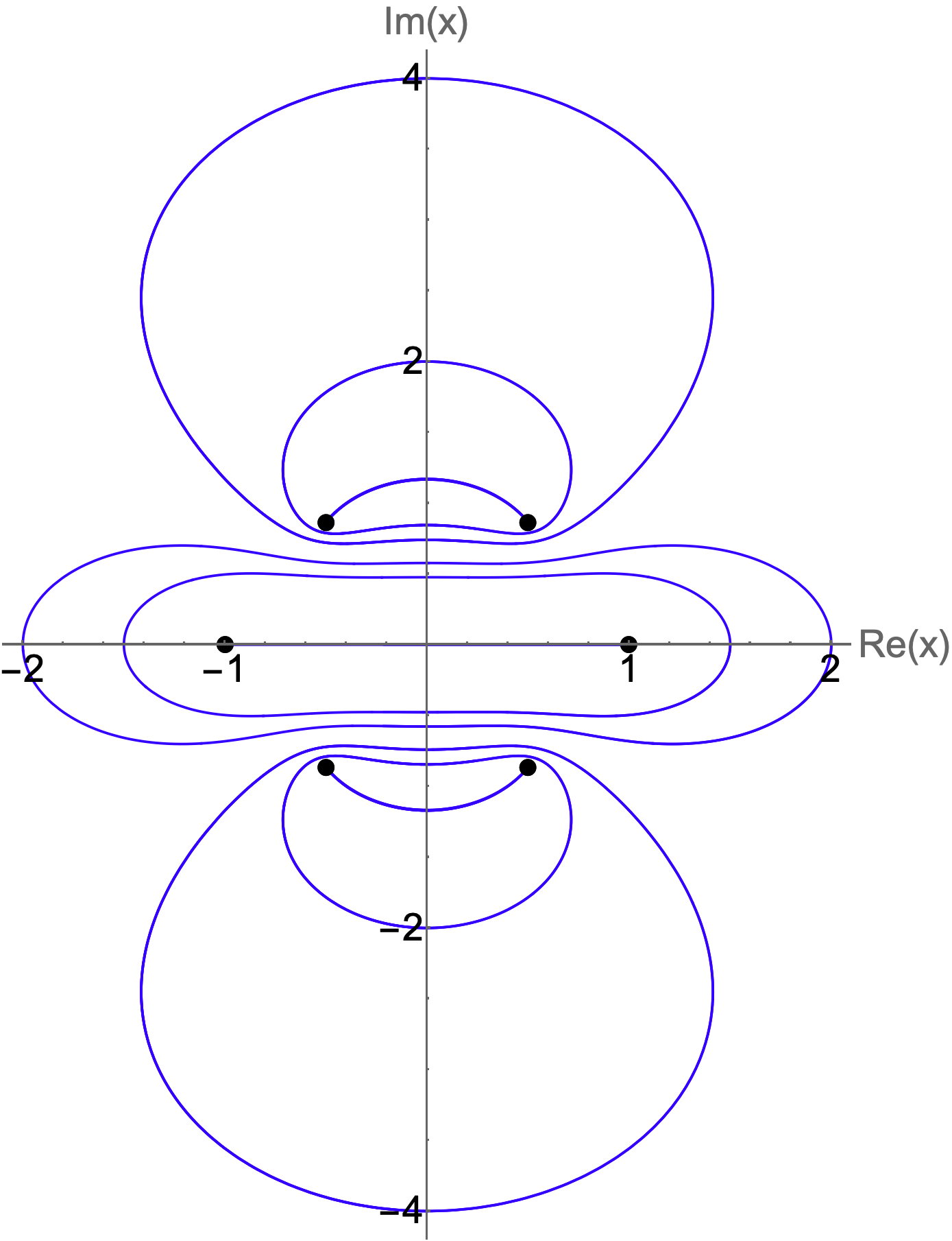
However, if the real line is embedded in the complex- plane, we observe a totally different classical behavior. We treat and as complex functions of the parameter . The classical equations of motion (1) determine the classical trajectories in the complex- plane (see Fig. 2).
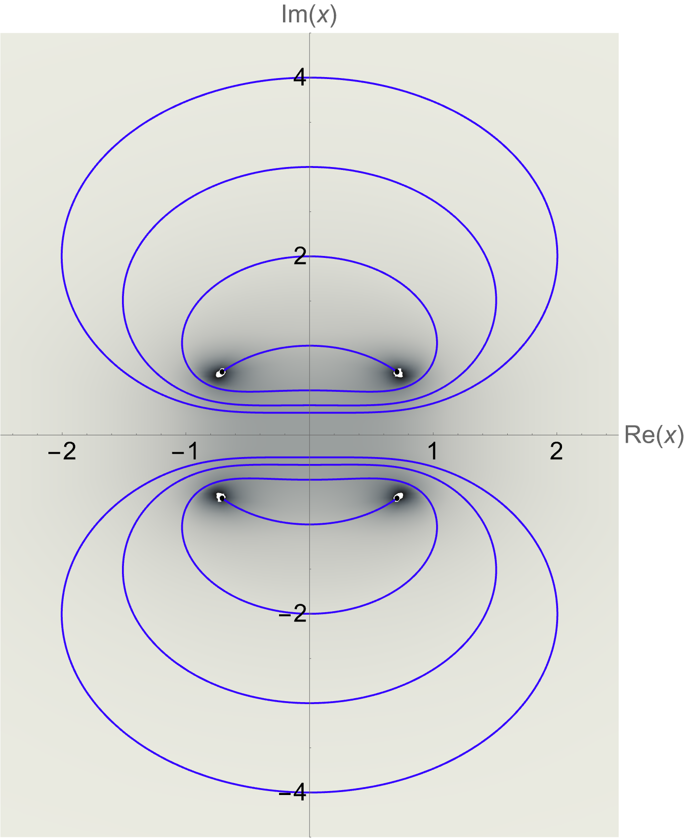
Figure 2 shows two pairs of classical turning points, one in the upper-half and the other in the lower-half complex- plane. A classical particle may oscillate between each pair of turning points. The other orbits are periodic and enclose the pairs of turning points. The real axis is a separatrix; no trajectories may cross the real axis. Large orbits are roughly D-shaped and in the limit as the orbits increase in size, one side of the orbit approaches the real axis while the other makes a huge semicircular sweep from to . Thus, a particle initially at the origin runs off to and then returns to the origin from .
As a consequence of Cauchy’s theorem and path independence, the period of every classical orbit in Fig. 2 is . Thus, particles in larger orbits move faster. If a particle starts at the origin, it zooms off to along the real- axis and it reaches infinity in time . It then returns to the origin from , again in time .
How did such a particle go from to in no time? The physical answer is that the particle travels at infinite speed at . The mathematical answer is that the point at complex is unique because the complex plane is compact; so, if the particle is at , it is already at . The stereographic image of this path is quite simple: The particle begins at the south pole, travels on a great circle up to the north pole, and then continues along the great circle back to the south pole. This particle never changes its direction of travel; if it leaves the origin traveling to the right, it returns to the origin still traveling to the right.
The real-world and complex-world dynamical behaviors of a classical particle are profoundly different. A classical particle traveling along the axis in the real plane is in an unbound state; it goes from the origin to and never comes back. This classical behavior resembles that of an unstable decaying quantum system located at :
| (3) |
However, in the complex plane all orbits are periodic and return to their initial positions:
| (4) |
This system is dynamically stable. Because the particle is statistically most likely to be found where it is traveling slowly, the complex motion resembles that of a localized quantum bound state. The classical probability of finding the particle near in the complex plane is peaked at and vanishes like for large (see [2]).
Particle trajectories corresponding to these real-unstable and complex-stable behaviors exhibit different global symmetries. In (3) particles on the negative-real line are left-moving and particles on the positive-real line are right-moving. These trajectories are parity symmetric; under reflection () right-moving particles for become left-moving particles for .
However, in the complex plane every trajectory is parity-time () symmetric. This is because space reflection replaces with and time reversal performs complex conjugation and thus it replaces with . Combined and changes the sign of , so performs a horizontal (left-right) reflection about the imaginary axis. (The direction of motion in each orbit is also reversed under this reflection because time reversal changes the sign of the velocity.)
While the operator performs a reflection about the imaginary axis, Hermitian conjugation (complex conjugation) is a reflection about the real axis. Thus, these are two orthogonal and independent symmetry operations. In the complex plane these symmetry operations are distinct from parity , which performs a reflection through the origin ().
3 Classical phases
The example above shows that one Hamiltonian may generate completely different kinds of classical-mechanical behaviors, which we refer to as phases. In one phase particles on the real axis escape to , as illustrated schematically in (3). This phase is characterized by having global symmetry. Classical trajectories in this phase are invariant under parity reflection.
In the second phase particles follow periodic orbits. On the real axis these particles run off to and come back from , as illustrated schematically in (4). This phase is globally symmetric. All trajectories in this phase are parity-time symmetric and particle trajectories on the real axis in this phase are said to be unidirectional [3].
4 Quantum phases
Quantum-mechanical Hamiltonians can also define multiple phases that are distinguished by having different global symmetries. For example, the quantum anharmonic-oscillator Hamiltonian with an upside-down quartic potential,
| (5) |
defines two phases. The time-independent Schrödinger equation associated with in (5) is
| (6) |
Physically observable solutions to (6) belong to two distinctly different phases because they obey different boundary conditions at . Depending on how the negative sign in front of the quartic term in is obtained, we get either a -symmetric phase with complex-energy eigenvalues and unstable states, or a -symmetric phase for which the energy spectrum is entirely real and positive, and the states are all stable.
To obtain the -symmetric phase of (5), we begin with the Hamiltonian for a quantum anharmonic oscillator with a right-side-up potential
| (7) |
The Hamiltonian (7) is parity symmetric; it is invariant under and . We construct the upside-down quartic Hamiltonian in (5) from in (7) by performing an analytic rotation in complex-coupling-constant space; that is, we let and rotate smoothly in the positive sense from to . Under this rotation the parity symmetry of in (7) is preserved.
We must perform this rotation carefully: As we increase , we must simultaneously rotate the boundary conditions on the eigenfunctions of in (7). We cannot solve the Schrödinger equation (6) exactly, but WKB theory provides an asymptotic approximation to for large , and thus WKB specifies the boundary conditions that the eigenfunctions obey as the rotation is performed [4].
When , the usual boundary conditions on the eigenfunctions are simply that as . However, the WKB approximation to specifies that the eigenfunctions vanish exponentially for large like . These eigenfunctions also vanish exponentially as in the complex- plane in a pair of wedge-shaped regions called Stokes sectors. These sectors are centered about the positive-real and negative-real axes and have an angular opening of . As increases from to , this pair of wedges rotates clockwise like a propeller by an angle of until at the upper edge of the right sector lies on the positive- axis and the lower edge of the left sector lies on the negative- axis.
We can also rotate in the negative sense from to . In this case the pair of Stokes sectors rotate anticlockwise by an angle of until the lower edge of the right sector lies on the positive- axis and the upper edge of the left sector lies on the negative- axis. Both the positive and negative rotations preserve the symmetry of the original Hamiltonian (7); during the rotation process the pair of Stokes sectors remains symmetric under a reflection through the origin in the complex- plane.
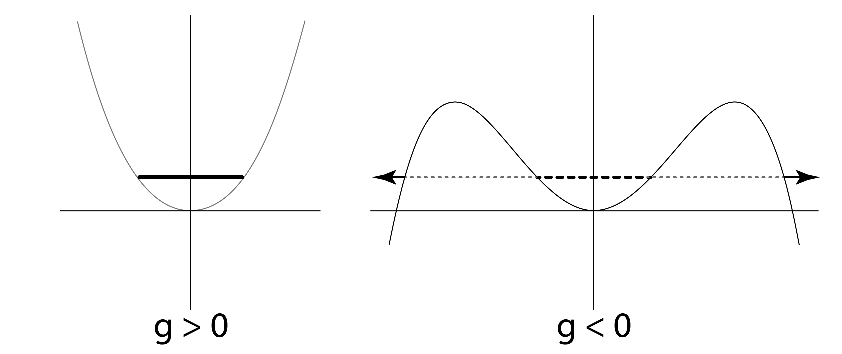
For both positive and negative rotations of , the edges of the Stokes sectors lie on the real- axis. This implies that the eigenfunction solutions to the Schrödinger equation (6) become wavelike (oscillatory). Depending on the choice of rotation direction, there are either outgoing-wave or incoming-wave solutions to the time-dependent Schrödinger equation. Figure 3 shows that a stable bound state in the right-side-up quartic potential (7) becomes unstable in the upside-down potential (5) and that the state tunnels outward to . This is the quantum analog of the classical behavior represented in (3).
We can obtain the -symmetric phase of the upside-down potential in (5) by performing a smooth complex deformation of the harmonic-oscillator Hamiltonian. To do so, we use the complex non-Hermitian Hamiltonian
| (8) |
This Hamiltonian is symmetric because a reflection changes the signs of the and and a reflection changes the signs of and . When , is the harmonic-oscillator Hamiltonian, which is both and symmetric. As we smoothly increase from 0 to 2, deforms into the Hamiltonian (5).
This smooth deformation breaks the symmetry but preserves the symmetry of the harmonic-oscillator Hamiltonian. The harmonic-oscillator eigenfunctions vanish in a pair of Stokes sectors of opening angle centered about the positive-real and negative-real axes. These sectors are invariant under both and reflections. However, as increases, both sectors rotate downward; the right sector rotates in the negative direction and the left sector rotates in the positive direction until the upper edge of each sector lies on the real axis. The opening angles of each sector shrink from to as increases from 0 to 2. The orientation of these sectors is no longer symmetric but remains (left-right) symmetric.
The schematic diagram in Fig. 4 shows that a real energy level in the right-side-up potential of at continues to be real when even though the potential is upside down. This is because the boundary conditions at are unidirectional [3, 5]. while the probability current flows out of the well on one side, there is an equal flow into the well on the other side, so the state in the potential well does not decay.

There is another way to perform a deformation of the harmonic oscillator that preserves the reality of the eigenvalues. Instead of deforming the Hamiltonian (8), we can deform the -symmetric Hamiltonian
| (9) |
by increasing smoothly from to . This deformation gives the same discrete positive-energy spectrum as in the defomation above, but the wave configurations are opposite to those shown in Fig. 4; there are incoming waves at and outgoing waves at . Each of these unidirectional wave configurations is separately invariant under reflection. The energy levels and wave configurations can be observed in laboratory experiments [5].
The -symmetric real-eigenvalue phase and the -symmetric complex-eigenvalue phase of the Hamiltonian (5) are distinct physically observable phases of the Hamiltonian 5). The positive-coupling Hamiltonian (7) has a positive-spectrum phase that is both - and -symmetric and the negative-coupling Hamiltonian (5) has a -symmetric phase with a positive spectrum, but these two spectra are different. One spectrum cannot be obtained from the other by analytic continuation in the coupling constant .
Furthermore, the Green’s functions of the two Hamiltonians are completely different. The odd- Green’s functions of the positive- theory vanish, but the odd- Green’s functions are nonzero for the negative- -symmetric theory [2].
The energy levels of the simpler Hamltonian
| (10) |
are plotted in Fig. 5 for . This is the earliest class of -symmetric Hamiltonians that was studied in detail [6]. For the eigenvalues of in (10) are all real, positive, and discrete. This property was first discovered in [6] and spectral reality was proved in [7].

Figure 5 indicates that there is a spectral transition at : When , some eigenvalues remain real but others occur in complex-conjugate pairs. (These complex eigenvalues are not shown in the figure.) This transition, which is called the transition, has been observed in many laboratory experiments involving different kinds of -symmetric physical systems (see refs. in [8]).
5 Quantum Hamiltonians with multiple phases
The number of phases defined by a quantum-mechanical Hamiltonian equals the number of pairs of Stokes sectors in which one can pose an eigenvalue problem for the Schrödinger equation associated with . For example, the cubic-potential Hamiltonian
| (11) |
has five Stokes sectors in the complex- plane in which the solutions to the Schrödinger equation
| (12) |
associated with can vanish exponentially as . These sectors are labeled in Fig. 6 as A, B, C, D, E.
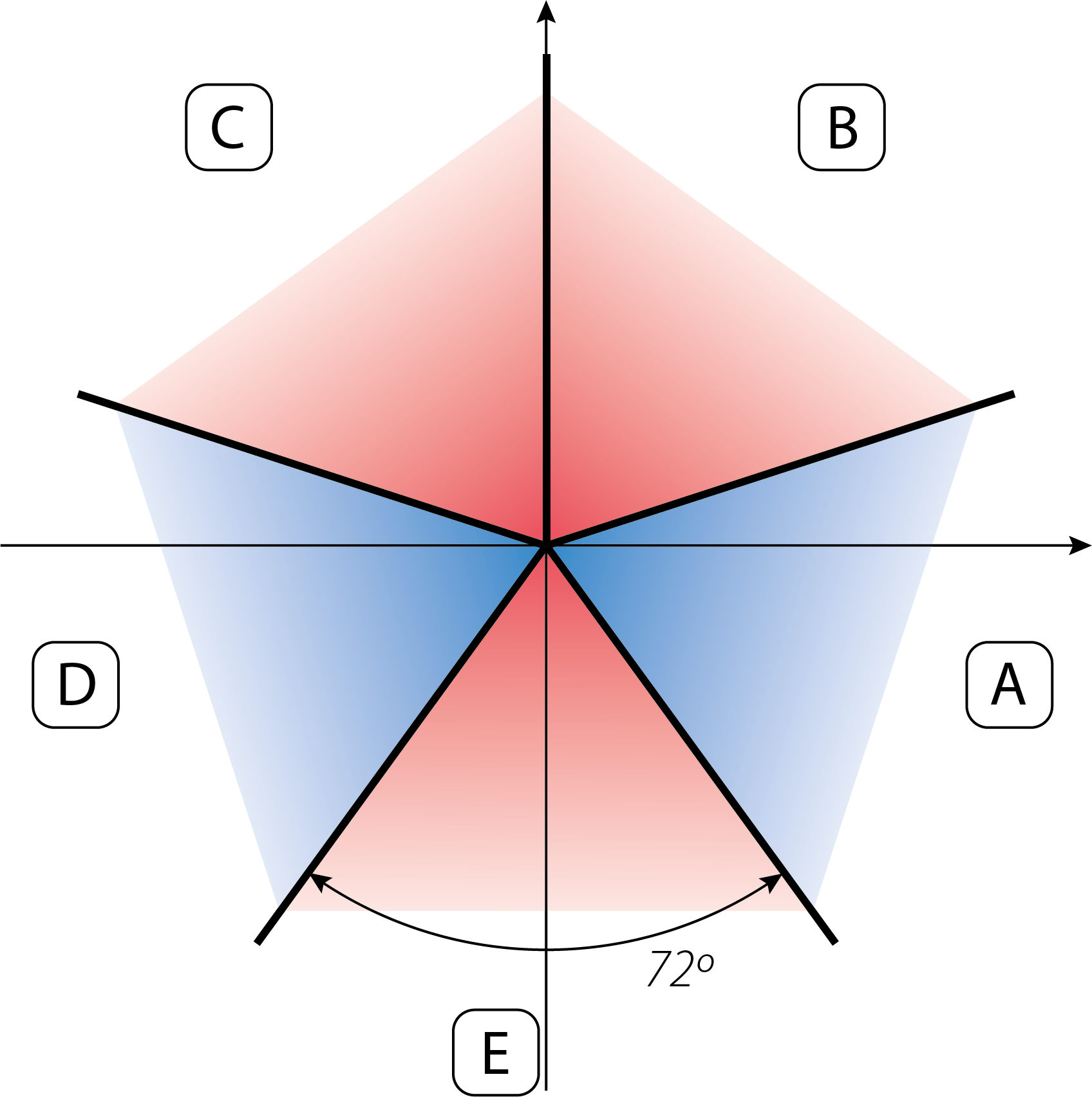
The eigenfunctions of in (11) must vanish exponentially in a pair of noncontiguous Stokes sectors. There are five such pairs of sectors: AC, AD, BD, BE, and CE. Thus, the Hamiltonian defines five different phases. Each of these phases has an countably infinite set of eigenfunctions and corresponding eigenvalues. However, the eigenvalue problem associated with the AD pair of sectors is special because the eigenvalues are all real and positive; this is because the AD pair of Stokes sectors is (left-right) symmetric. These real eigenvalues are shown in Fig. 5 for the value . The eigenvalues associated the other four phases are all complex.
Next, consider the sextic Hamiltonian
| (13) |
There are eight Stokes sectors in the complex- plane in which the solutions to the Schrödinger equation
| (14) |
associated with can vanish like as . The angular opening of each sector is . The sectors are shown in Fig. 7 and are labeled A, B, , H.
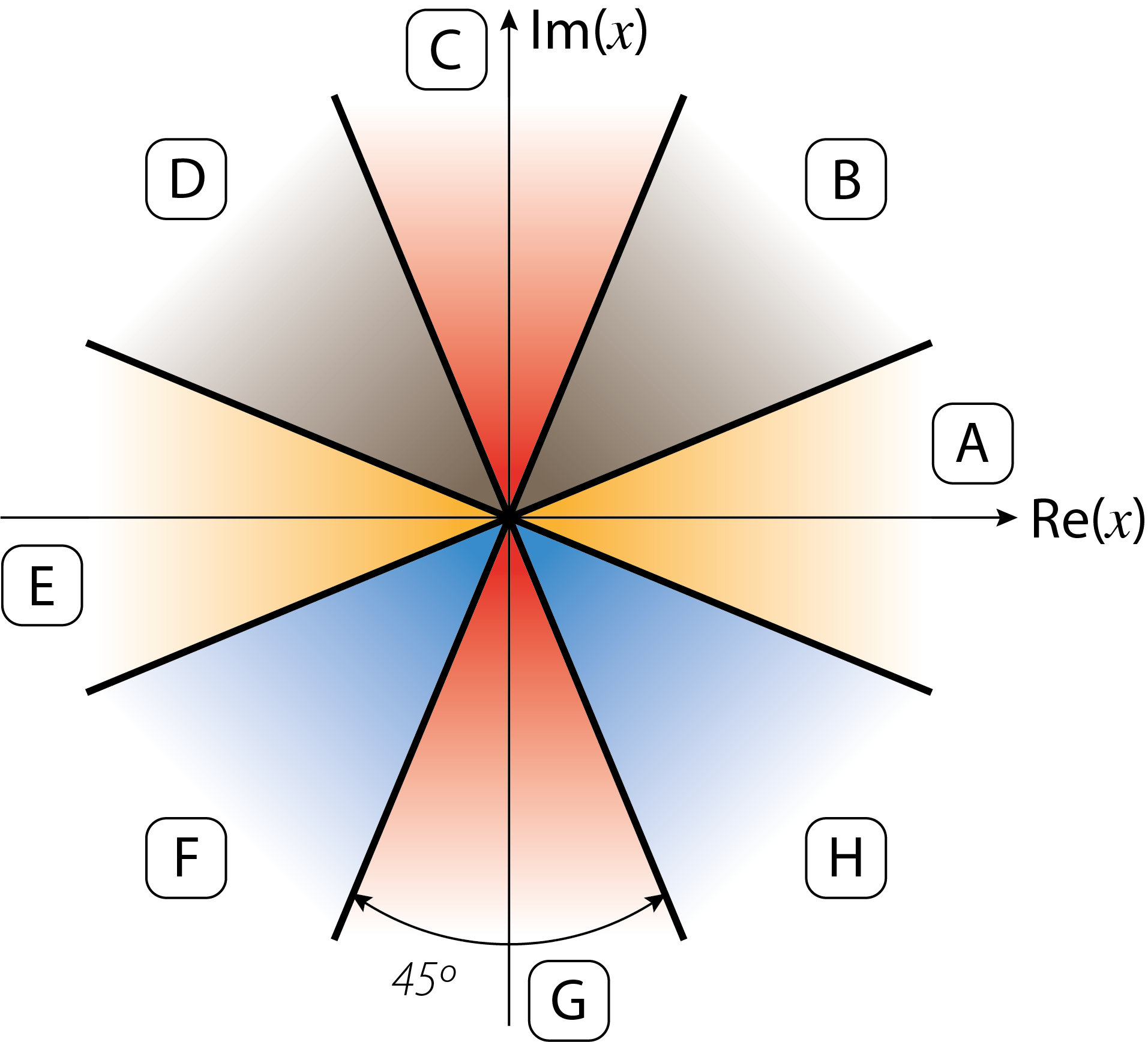
The lowest five eigenvalues in the Hermitan AE sectors are approximately , , , , and , and the lowest five eigenvalues in the -symmetric BD and FH sectors are , , , , and . WKB analysis reveals that for high energies the -symmetric eigenvalues are larger than the Hermitian eigenvalues by a factor of . This feature might be analogous to families of particles having similar physical properties, such as the electron, muon, and tau, that have increasingly larger masses [9].
6 Relationship between classical and quantum phases
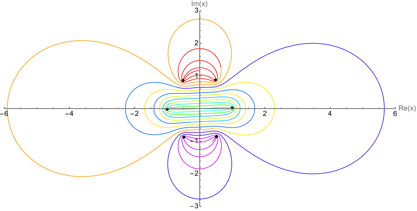
The three positive-energy quantum phases of in (13) have a clear classical analog. Figure 9 gives a plot of the classsical paths corresponding to . Corresponding to the three left-right-symmetric pairs of quantum stokes sectors, there are three left-right-symmetric phases of classical paths. These phases fill the entire complex- plane and are bounded by separatrix paths.
There are also three phases of classical paths having corresponding to negative quantum energies. These phases are oriented vertically, corresponding to the vertical pairs of Stokes sectors BH, CG, and DF in Fig. 7 and are bounded by separatrix paths.
7 Phase transitions
For want of a better term, we use the term phases to describe the distinct sets of eigenfunctions and corresponding eigenvalues of a Hamiltonian. It is not yet clear if there is an order parameter that can be used to characterize these phases and if there are phase transitions. However, at the classical level one can arrange for particles in one phase to visit another phase. If the classical energy is complex, particle trajectories are no longer closed. Trajectories unwind and enter other phases, as shown in Fig. 9. (The average time for a classical particle to enter and leave a phase is proportional to , which is a classical analog of the time-energy uncertainty principle.) At the quantum level there are relationships between corresponding energy levels in different phases. For example, for in (11), if is the th energy level in the th phase, then .
8 -symmetric quantum theory
In a phase in which the spectrum is entirely real and positive one can formulate a fully consistent quantum-mechanical theory that is based on a -symmetric Hamiltonian instead of a Hermitian Hamiltonian [2, 6, 8]. Specifically, one can construct a Hilbert space of states with an appropriate positive-definite inner product. For example, there is a phase in which all of the energy levels of the deformed Hamiltonians in (10) are real and positive if (see Fig. 5). Thus, despite its non-Hermiticity, defines a physically acceptable quantum-mechanical system.
9 -symmetric quantum field theory
This multiple-phase phenomenon extends from quantum mechanics to quantum field theory. For example, a quantum field theory appears to have two phases, an unstable -symmetric phase for scalar and a stable -symmetric phase for pseudoscalar . The theory is not asymptotically free, but the -symmetric theory is asymptotically free [10, 11].
Another example of a -symmetric quantum field theory is lurking in the classic 1952 paper on the divergence of perturbation series in quantum electrodynamics (QED) [12]). This paper argued heuristically that a perturbation series in powers of the fine-structure constant must diverge because if were replaced by , electrons and positrons would repel and the vacuum state would become unstable. Thus, the nature of the physics would change discontinuously at . The conclusion of this argument is correct, as shown in subsequent research [13, 14, 15, 16, 17], but the mathematical reason for this divergence is simply that the number of Feynman diagrams grows factorially with the order of perturbation theory.
There is an important subtlety not considered in Ref. [12]. Like the anharmonic-oscillator Hamiltonian (5), the negative sign of in QED leads to two phases, (1) a -symmetric phase (PQED) with an unstable vacuum state, and (2) a non-Hermitian -symmetric phase (PTQED) in which is an axial-vector field [18]. Unlike conventional Hermitian QED, the PTQED phase is asymptotically free and appears to have a stable vacuum state.
The program of Johnson, Baker, and Willey for calculating in massless QED failed because QED is not asymptotically free, as shown by the absence of a convergent sequence of positive zeros in the weak-coupling expansion of (the logarithmic-divergent part of the Beta function) [19, 20, 21]:
Even if this series is converted to Padé approximants [22, 20, 21, 23, 24, 25], no sequence of positive zeros emerges. However, for massless PTQED does appear to have a convergent sequence of negative zeros , which suggests that PTQED has an asymptotically free phase that is fundamentally different from Hermitian QED [26].
Studies of the Casimir force support the possibility that QED has a PTQED phase. In QED a conducting spherical shell experiences a repulsive Casimir force that tends to inflate the sphere [27]. However, in PTQED a conducting spherical shell tends to collapse. If this attractive force is balanced by placing an electric charge on the shell, one obtains the approximate negative [26].
10 Concluding remarks
Even though these field-theory results are not rigorous, it is now clear that studies of quantum theory in the complex domain will continue to reveal a rich array of new, unexpected, and experimentally observable behaviors.
Acknowledgements.
CMB thanks the Alexander von Humboldt and Simons Foundations for financial support.References
- [1] \NameBender C. M. Hook D. W. \REVIEWJournal of Physics A: Mathematical and Theoretical41200824405.
- [2] \NameBender C. M., Dorey P. E., Dunning C., Fring A., Hook D. W., Jones H. F., Kuzhel S., Lévai G. Tateo R. \BookPT Symmetry in Quantum and Classical Physics (World Scientific, Singapore) 2019.
- [3] \NameRamezani H., Kottos T., El-Ganainy R. Christodoulides D. N. \REVIEWPhysical Review A822010043803.
- [4] \NameBender C. M. Wu T. T. \REVIEWPhysical Review18419691231.
- [5] \NameSoley M. B., Bender C. M. Stone A. D. \REVIEWPhysical Review Letters1302023250404.
- [6] \NameBender C. M. Boettcher S. \REVIEWPhysical Review Letters8019985243.
- [7] \NameDorey P., Dunning C. Tateo R. \REVIEWJournal of Physics A: Mathematical and General3420015679.
- [8] \NameBender C. M. Hook D. W. \REVIEWArXiv20232312.17386.
- [9] \NameBender C. M. Klevansky S. P. \REVIEWPhysical Review Letters1052010031601.
- [10] \NameSymanzik K. \REVIEWCommunications in Mathematical Physics45197579.
- [11] \NameBender C. M., Duncan A. Jones H. F. \REVIEWPhysical Review D4919944219.
- [12] \NameDyson F. J. \REVIEWPhysical Review851952631.
- [13] \NameHurst C. A. \REVIEWMathematical Proceedings of the Cambridge Philosophical Society481952625.
- [14] \NamePetermann A. \REVIEWPhysical Review8919531160.
- [15] \NameThirring W. \REVIEWHelvetica Physica Acta26195333.
- [16] \NameGlimm J. Jaffe A. \REVIEWPhysical Review17619681945.
- [17] \NameBender C. M. Wu T. T. \REVIEWPhysical Review Letters271971461.
- [18] \NameBender C. M., Cavero-Palaez I., Milton K. A. Shajesh K. V. \REVIEWPhysics Letters B613200597.
- [19] \NameJost R. Luttinger J. M. \REVIEWHelvetica Physica Acta231950201.
- [20] \NameRosner J. L. \REVIEWAnnals of Physics44196711.
- [21] \NameGorishny S. G., Kataev A. L., Larin S. A. Surguladze L. R. \REVIEWPhysics Letters B256199181.
- [22] \NameRosner J. \REVIEWPhysical Review Letters1719661190.
- [23] \NameJohnson K., Baker M. Willey R. S. \REVIEWPhysical Review Letters111963518.
- [24] \NameJohnson K., Baker M. Willey R. \REVIEWPhysical Review1361964B1111.
- [25] \NameJohnson K., Baker M. Willey R. \REVIEWPhysical Review16319671699.
- [26] \NameBender C. M. Milton K. A. \REVIEWJournal of Physics A: Mathematical and General321999L87.
- [27] \NameBoyer T. H. \REVIEWPhysical Review17419681764.