LLM meets Vision-Language Models for Zero-Shot One-Class Classification

Abstract

We consider the problem of zero-shot one-class visual classification. In this setting, only the label of the target class is available, and the goal is to discriminate between positive and negative query samples without requiring any validation example from the target task. We propose a two-step solution that first queries large language models for visually confusing objects and then relies on vision-language pre-trained models (e.g., CLIP) to perform classification. By adapting large-scale vision benchmarks, we demonstrate the ability of the proposed method to outperform adapted off-the-shelf alternatives in this setting. Namely, we propose a realistic benchmark where negative query samples are drawn from the same original dataset as positive ones, including a granularity-controlled version of iNaturalist, where negative samples are at a fixed distance in the taxonomy tree from the positive ones. Our work shows that it is possible to discriminate between a single category and other semantically related ones using only its label. Our code is available online: https://github.com/ybendou/one-class-ZS

1 Introduction

Recently, the literature has shown the feasibility of classifying visual objects in a zero-shot fashion, where only class labels (or a textual description) are leveraged to infer a classifier on images [33, 44]. These approaches make use of vision-language pre-trained models such as CLIP [33] that align text and images, showing good performance in datasets containing from ten to hundreds of classes [48, 24]. In this paper, we are interested in the limit case of identifying a single category (i.e., one-class classification), which finds its utility in various domains, including anomaly detection, fraud prevention, image quality assessment, etc. Interestingly, existing zero-shot classification approaches are not easily adapted to this limit case, since they typically require multiple categories to build their classifiers.

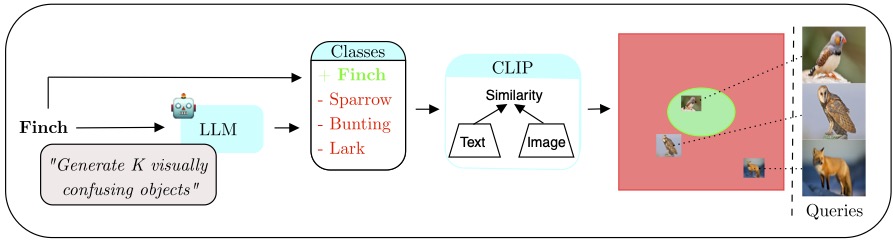
(a)

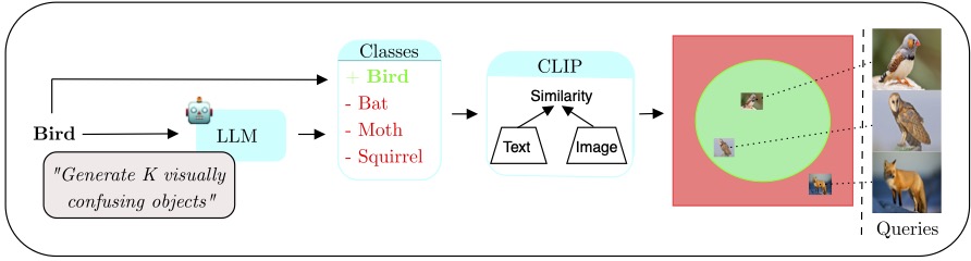
(b)

Figure 1: Illustration of the proposed method for two instances of a zero-shot one-class classification task, where only the class label is given. In the first case (a), only the “Finch” example is identified as a “Finch”. In the second scenario (b), both bird examples are classified as birds. Negative examples of classes are obtained through querying an LLM. Notice that the position of query images is unchanged between the two instances, as only the class boundaries vary.

The task of classifying multiple objects typically involves estimating the boundaries between classes. The challenge with one-class classification, however, lies in defining these boundaries solely based on examples from the class in question. Other settings exist, where negative examples are provided [25, 17], thus helping estimate this boundary. Recent works also consider the case of zero-shot out of distribution [27, 43, 10], mainly reporting AUC scores where the exact boundary estimation, through the use of an explicit threshold, is not directly addressed. However, we argue that validation samples are not necessarily available in practice, particularly in zero-shot classification, and that the question of finding the absolute position of the boundary still holds untapped potential.

In this paper, we aim to show that it is possible to define performing one-class classifiers using a single class label. We propose a methodology that combines vision-language pre-trained models with Large Language Models (LLMs) in a two-step procedure, where the LLM is used to suggest names of visually confusing categories that are incorporated to estimate the boundary of the target class (c.f. Figure 1). To illustrate, consider the classification of the class “Finch”. Our method would prompt an LLM to identify closely related categories, such as “Sparrow” or “Canary” which, while similar, are not finches. This nuanced differentiation is crucial for accurately defining the boundary of the “Finch” class. We extend this approach to more general categories, such as “Bird” demonstrating our methodology’s effectiveness across varying levels of specificity.

We validate our methodology on existing large-scale vision datasets adapted for zero-shot one-class classification. Our contributions are as follows:

1. To the best of our knowledge, we are the first to tackle the problem of zero-shot one-class classification, where only the label of the class of interest is available;

2. We propose a realistic benchmark where negative query samples are drawn from the same original dataset as positive ones, including a granularity-controlled version of iNaturalist, where negative samples are at a fixed distance in the taxonomy tree from the positive ones;

3. We propose a methodology making use of an LLM and a vision-language pre-trained model. We conduct extensive experiments to demonstrate the robustness of our approach across a diverse range of tasks, showing its benefits compared to adapted off-the-shelf alternatives.

2 Preliminaries

Problem Statement

Let us formally define the zero-shot one-class classification task: the goal is to learn a classification function $\psi_{\mathbf{t}}(\mathbf{x})$ that maps an input $\mathbf{x}$ to its label $y\in\{0,1\}$ using only the text $\mathbf{t}$ of the target class.

Our objective is to build a binary classifier that aims at maximizing the macro F1 score, defined as $\text{F1}_{\text{macro}}=\frac{\text{F1}_{+}+\text{F1}_{-}}{2}$, where $\text{F1}_{+}$ and $\text{F1}_{-}$ are the F1 scores of the positive and negative classes respectively. This is a classical measure of performance in one-class classification and out-of-distribution detection [16].

We expect positive and negative samples to be drawn from very different underlying distributions, since positive samples typically represent a single category, whereas negatives can be drawn from multiple other – near or far – categories. This asymmetry is important, as it suggests the use of classifiers where positive and negative class domains can be very different.

Vision-Language Pre-Training

In recent years, visual language models have gained traction, integrating text and images for more effective learning. Contemporary models like CLIP [33] and ALIGN [18] use a contrastive learning framework, showing impressive multi-class zero-shot learning capabilities without additional fine-tuning. CLIP demonstrates a straightforward yet powerful approach by training a double encoder network $\mathcal{T}\colon\mathbf{t}\mapsto\mathbf{w}\in\mathbb{R}^{d}$ and $\mathcal{I}\colon\mathbf{x}\mapsto\mathbf{v}\in\mathbb{R}^{d}$ to embed text and images respectively, in a shared embedded space. By treating the class label as a class prototype, this approach allows to compute a cosine similarity score between images and texts embeddings for zero-shot classification defined as follows: $s(\mathbf{x},\mathbf{t})=\frac{\mathcal{I}(\mathbf{x})^{\top}\mathcal{T}(\mathbf{t})}{\|\mathcal{I}(\mathbf{x})\|\|\mathcal{T}(\mathbf{t})\|}$.

Building classifiers based on cosine similarity results in operating on the hypersphere, leading to a diverse array of methods for class discrimination based on geometric considerations, as discussed in the next section.

3 Methodology

We build a binary classifier using the cosine similarity between the target class $\mathbf{t}$ and the query image $\mathbf{x}$, leveraging the fact the text embedding is often used as a class prototype in zero-shot classification [33]. Formally, denoting $\lambda_{\mathbf{t}}(\mathbf{x})$ a threshold, the zero-shot one-class classification is performed as:

$$\psi_{\mathbf{t}}(\mathbf{x})=\left\{\begin{array}[]{ll}1\quad\text{if}\quad s(\mathbf{x},\mathbf{t})\geq\lambda_{\mathbf{t}}(\mathbf{x}),\\ 0\quad\text{otherwise}\end{array}\right.$$ (3)

We envision multiple ways to define the threshold $\lambda_{\mathbf{t}}(\mathbf{x})$:

• Fixed thresholding: When constant in $\mathbf{x}$, this approach creates a decision boundary dividing the hypersphere, a classification space formed by the cosine similarity, into two hemispheres based on similarity to text $\mathbf{t}$;

• Adaptive thresholding: It can be dependent in $\mathbf{x}$, leading to two considered solutions. The first approach defines the domain of the positive class as a single Voronoï cell, based on cosine similarity. The second one involves decision boundaries that acts as a hyperplane, positioned equidistantly in terms of cosine similarity from the prototypes of two classes.

Fixed Thresholding

The first method we consider consists in using a single threshold for all tasks, leading to a constant radius for the boundary sphere in $\psi_{\mathbf{t}}$. Given that we do not have a validation set for the downstream task, we propose to use ImageNet1K to compute an average threshold from a large number of artificially generated tasks. Note that this dataset is often used for selecting hyperparameters in multi-class zero-shot classification [6, 41]. We conduct experiments to show the impact of selecting the threshold from different datasets in the supplementary material. This threshold is the one which maximizes the F1-score over $1000$ one-class tasks. We refer to this first method as Fixed Thresholding (FT).

Our experiments show that, while fixing a single threshold $\bar{\lambda}$ for all tasks is a reasonable baseline in some cases, an optimal threshold for a certain task may fail for other tasks, especially for scenarios that are far from the average ImageNet1K ranges. In fact, different classes can have different cosine similarities with their class labels, as well as different ranges. We showcase this effect later in the paper in Figure 5 where we plot the distribution of the optimal thresholds for various tasks, motivating the need for an adaptive threshold method.

Adaptive Thresholding

In order to obtain adaptive boundary decisions, recent methods proposed to use a negative prototype estimated from available positive data [16]. The aim is to obtain a negative prototype such that the negative examples match it more than the target class. In the zero-shot setting, we draw inspiration from [16] to obtain negative prototypes using a LLM. To do so, given a target class name, we prompt GPT-4 [1] to obtain $K$ labels that could be visually confused with the target class. Our hypothesis is that LLMs capture a large amount of knowledge including the class perimeter. Alternatively, this task could be done by an expert to identify the semantically closest classes.

We refer to the $K$ visually confusing objects $(\mathbf{t}_{n_{1}},\dots,\mathbf{t}_{n_{K}})$. We then propose two methods to exploit them:

• The first one is to compute $K$ thresholds and take their maximum, which we call Multi Negative Prototype (MNP). This method boils down to performing multi-class classification between $K+1$ classes:

  $$\lambda_{\mathbf{t}}(\mathbf{x})~{}=~{}\max_{k\in\{1\dots K\}}\frac{\mathcal{I}(\mathbf{x})^{\top}\mathcal{T}(\mathbf{t}_{n_{k}})}{\|\mathcal{I}(\mathbf{x})\|\|\mathcal{T}(\mathbf{t}_{n_{k}})\|}$$ (4)

  In other words, the MNP method associates the target class and each LLM-generated confusing object with its own Voronoï cell;

• The second one estimates an average negative prototype: $\bar{\mathbf{w}}~{}=~{}\sum_{i=1}^{K}{\frac{\mathcal{T}\left(\mathbf{t}_{n_{i}}\right)}{K}}$ then computes the threshold as follows:

  $$\lambda_{\mathbf{t}}(\mathbf{x})=\frac{\mathcal{I}(\mathbf{x})^{\top}\bar{\mathbf{w}}}{\|\mathcal{I}(\mathbf{x})\|\|\bar{\mathbf{w}}\|}$$ (5)

  Here, $\psi_{\mathbf{t}}$ becomes a binary linear classifier. We refer to this method as Average Negative Prototype (ANP) in the remaining of this work.

Adaptive $+$ Fixed Thresholding

In the adaptive thresholding approach, the decision to classify a sample as positive is fundamentally based on its similarity(es) from the negative prototype(s). Essentially, if a sample is distant from all negative prototypes, it is deemed positive, regardless of its absolute closeness to the positive class prototype—provided it is closer to the positive than to the negatives. In other words, the adaptive approaches do not inherently constrain positive samples within a specific region relative to the positive class prototype. This characteristic can lead to a broader, less precise definition of the positive class, potentially including outliers or marginally related samples in the positive classification. To address this limitation, we propose combining adaptive and fixed thresholding methods. This hybrid approach aims to refine the classification by incorporating the fixed threshold obtained from ImageNet1K ($\bar{\lambda}$) alongside the adaptive thresholding:

$$\bar{\lambda}_{\mathbf{t}}(\mathbf{x})=\frac{1}{2}\lambda_{\mathbf{t}}(\mathbf{x})+\frac{1}{2}\bar{\lambda}$$ (6)

This combined threshold serves to more precisely delineate the positive class, restricting it to a more defined region. By doing so, this method ensures that samples are classified as positive not only by being distant from the negative prototypes but also by being genuinely close to the positive class prototype.

Considering the typically positive nature of cosine similarities between text and image representations in CLIP [22], natural images $\mathbf{x}$ satisfy the following: $\bar{\lambda}_{\mathbf{t}}(\mathbf{x})\geq\frac{1}{2}\bar{\lambda}$. Accordingly, the positive classification is effectively bounded within a region exhibiting a higher similarity than $\frac{1}{2}\bar{\lambda}$, ensuring a more precise and restrictive definition of the positive class.

4 Proposed Benchmark

A simple way to generate realistic one-class classification benchmarks consists in using existing classification vision datasets, randomly selecting a class to be our target, and sampling positive and negative examples from respectively the target class and the other ones. We call this sampling “uniform”. However, by doing so we do not have explicit control over the granularity of the generated tasks. We thus also propose a “hierarchical” sampling based on the taxonomy of the iNaturalist dataset allowing to control the proximity between positive and negative examples. More details are provided thereafter.

4.1 Uniform Sampling

We adapt existing large-scale vision classification datasets for one-class zero-shot classification. We first sample a target class $c$ uniformly at random. We then sample 100 images with a ratio of positive samples $r$, uniformly among the positive samples from class $c$ or negative samples from any other class.

4.2 Hierarchical Sampling

We also adapt the hierarchical iNaturalist [42] dataset to produce tasks with varying levels of granularity. iNaturalist hierarchy forms a tree that begins with the most inclusive categories (i.e., “Kingdoms”) which encompass broad groups such as plants, animals, and fungi. From there, it progressively narrows down through various levels of specificity, culminating in the individual species that constitute the ten thousands of leaves of the tree.

Considering a level of granularity $L$, we generate tasks by first selecting a leaf uniformly at random in the tree. Its $L$-th ancestor becomes the class of positive examples, and its $L+1$-th ancestor, deprived of the $L$-th ancestor, becomes the class of negative examples. We justify this choice because given the extensive diversity of classes, we aim to prevent the selection of negative queries that are too distantly related to the target class, as this would result in overly simplistic tasks such as discriminating between a cell and a dog. The proposed sampling creates hard tasks that we believe to be realistic. Finally, for each task, we sample 100 queries with a fixed ratio of positive samples $r$.

5 Experimental Setup

5.1 Datasets and Metrics

In our experiments, we employ the hierarchical sampling for iNaturalist and the uniform sampling for 5 existing datasets: EuroSAT [13], Food [2], SUN [45], Textures [8] and Pets[31]. We sample 100 queries per task and report the performance over 1,000 runs. The ratio of positive samples is set at $r=0.5$, unless specified otherwise. We primarily report our results using the macro F1-score, a classical measure in the field of out-of-distribution detection. To provide a broader picture of our methods’ effectiveness, we also report the AUC score in the supplementary material as well as the accuracy for cases with balanced data.

5.2 Architectures and Baselines

In terms of architecture, we employ three pre-trained models. We use the ViT-B-16 and ViT-B-32 from CLIP [33], commonly used for zero-shot tasks and allowing comparison with previous work. The third architecture is the Open-CLIP ViT-H-14 [7], a more recent and capable pretrained vision-language model.

Our approach is benchmarked against two existing alternatives from zero-shot out-of-distribution (OOD) detection domain which we adapt to the zero-shot one-class case. The first method is CLIPN, a variant of CLIP enhanced to generate negative prompts using the template “a photo of no <class>” [43]. The second approach is ZOC[10] which uses a fine-tuned BERT decoder on COCO dataset [23] to generate class candidates potentially present in the query image. These two methods generate negative prototypes which could be seen as an alternative to the adaptive threshold module, therefore we propose to combine them with the fixed thresholding regularization resulting in CLIPN+FT and ZOC+FT. We directly use the shared models from the original papers in our experiments. We also investigate the impact of the choice of the negative prototypes by further including in the supplementary material results using the class labels available in the original dataset.

5.3 Implementation Details

For textual embeddings extraction from CLIP, we use the template “a photo of a <class>”. Furthermore, the use of scientific names in the iNaturalist dataset has been demonstrated to yield suboptimal results, as models like CLIP were predominantly trained on common names [30]. Similarly to previous work [30], to address this, we opt for common names obtained using GPT4 in our experiments. We include in the supplementary material a comparison between common and scientific names, with common class names standardized across all compared methods for fairness. We query the considered LLM for generating 10 negative prototypes, which is discussed in Figure 4.b.

Regarding the fixed threshold from ImageNet1K, we generate 1000 tasks using the uniform sampling and compute the optimal threshold which maximizes the macro F1 score. The selected threshold is then the average across these tasks.

6 Results

6.1 Performance

We compare our proposed method (ANP+FT) with other alternatives in Table 1, using the models from the original papers. We observe that our proposed method achieves state-of-the-art performance across all of the considered datasets and backbones, with the noticeable exception of EuroSAT on VIT-B-32 – which can be explained by its low-resolution images – resulting in a significant gain in average compared to considered baselines. Using the larger OpenCLIP architecture, all results are significantly better, which justifies the use of this configuration for further experiments. It is noteworthy to add that ZOC requires significantly more computations at inference time since it uses an additional BERT decoder for each query image.

Table 1: Average macro F1 score for multiple datasets.

Backbone	Method	iNat	SUN	Food	Textures	Pets	EuroSAT	Average
ViT-B-16 CLIP	CLIPN [43]	$41.95\pm 0.79$	$85.66\pm 0.47$	$69.86\pm 0.77$	$52.28\pm 0.67$	$73.84\pm 0.76$	$60.67\pm 0.90$	$64.05$
	ANP+FT (ours)	$\mathbf{60.64\pm 1.02}$	$\mathbf{94.35\pm 0.36}$	$\mathbf{95.62\pm 0.17}$	$\mathbf{77.24\pm 1.09}$	$\mathbf{93.46\pm 0.81}$	$\mathbf{65.95\pm 0.91}$	$\mathbf{81.20}$
ViT-B-32 CLIP	ZOC[10]	$55.05\pm 0.99$	$93.61\pm 0.32$	$92.18\pm 0.24$	$73.88\pm 0.66$	$88.53\pm 0.77$	$\mathbf{65.38\pm 1.14}$	$78.16$
	ANP+FT (ours)	$\mathbf{60.32\pm 0.99}$	$\mathbf{94.19\pm 0.38}$	$\mathbf{94.18\pm 0.20}$	$\mathbf{78.21\pm 0.88}$	$\mathbf{90.97\pm 0.88}$	$59.72\pm 0.98$	$\mathbf{79.60}$
OpenCLIP	ANP+FT (ours)	${62.94\pm 1.11}$	$96.88\pm 0.25$	${97.52\pm 0.12}$	${86.64\pm 0.88}$	${96.69\pm 0.21}$	${74.51\pm 1.17}$	${85.86}$

We then report the performance of CLIPN and ZOC when combined with FT in Table 2. We observe a significant improvement of $15.57\%$ for CLIPN. On the other hand, ZOC benefits less from the regularization with varying gains depending on each dataset. We think it can be explained by the fact that while CLIPN and our method generate negative prototypes from the target class, ZOC generates the negative prototypes from the query images which can make ZOC less sensitive to false positives, limiting the necessity of constraining positive predictions in a high cosine similarity region.

Table 2: Effect of regularization for existing baselines. Average macro F1 score.

Backbone	Method	iNat	SUN	Food	Textures	Pets	EuroSAT	Average
ViT-B-16 CLIP	CLIPN [43]	$41.95\pm 0.79$	$85.66\pm 0.47$	$69.86\pm 0.77$	$52.28\pm 0.67$	$73.84\pm 0.76$	$60.67\pm 0.90$	$64.05$
	CLIPN[43] + FT	$50.77\pm 1.11$	$\mathbf{96.59\pm 0.16}$	$92.18\pm 0.31$	$76.70\pm 0.79$	$89.50\pm 0.52$	$\mathbf{72.03\pm 1.21}$	$79.62$
	ANP+FT	$\mathbf{60.64\pm 1.02}$	$94.35\pm 0.36$	$\mathbf{95.62\pm 0.17}$	$\mathbf{77.24\pm 1.09}$	$\mathbf{93.46\pm 0.81}$	$65.95\pm 0.91$	$\mathbf{81.20}$
ViT-B-32 CLIP	ZOC[10]	$55.05\pm 0.99$	$93.61\pm 0.32$	$92.18\pm 0.24$	$73.88\pm 0.66$	$88.53\pm 0.77$	$\mathbf{65.38\pm 1.14}$	$78.16$
	ZOC[10]+FT	$53.78\pm 0.10$	$\mathbf{95.30\pm 0.28}$	$93.74\pm 0.21$	${77.51\pm 0.68}$	$87.91\pm 0.76$	$64.82\pm 1.05$	$78.43$
	ANP+FT	$\mathbf{60.32\pm 0.99}$	$94.19\pm 0.38$	$\mathbf{94.18\pm 0.20}$	$\mathbf{78.21\pm 0.88}$	$\mathbf{90.97\pm 0.88}$	$59.72\pm 0.98$	$\mathbf{79.60}$

6.1.1 How does granularity affect performance?

In order to better understand the effect of varying the task granularity, we report the performance on iNaturalist per level in Figure 2. Note that a lower level means a fine-grained classification between very similar species, while higher levels represent larger concepts. Our results show that our method outperforms both CLIPN and ZOC as well as their regularized versions. While ZOC is competitive on some levels (2 and 3), our method significantly outperforms it on other levels with higher or lower granularity. Generating negative prototypes using a Large Language Model allows to effectively capture different levels of granularity. On the other hand, negative prototypes generated using ZOC are limited to the corpus of COCO on which it was fine-tuned, particularly for fine-grained tasks (e.g., discriminating between “Mugwort” and “Sagebrush”) which requires specific knowledge of the task. We provide in the supplementary material some visual examples showcasing the difficulty of our proposed setting.

(a) ViT-B-16 CLIP

(b) ViT-B-32 CLIP

Figure 2: Macro F1 score per level in iNaturalist for different backbones.

6.1.2 How well does a fixed threshold transfer from ImageNet1K?

Figure 3: Impact of varying the fixed threshold, for each dataset. We report the relative macro F1 score to the one obtained using the ImageNet1K threshold. For iNaturalist, we report the performance per level of granularity.

In order to investigate the transferability of a fixed threshold from ImageNet1K to other datasets, we run an analysis reported in Figure 3 where we vary the selected threshold and report its relative macro F1 score to the FT method. For iNaturalist, we report the performance per level. We observe that a single threshold is not optimal across different datasets. For iNaturalist, the wider the concept is, the lower are the similarities between images and the class labels. In contrast, fine-grained tasks tend to have high similarities with their class labels. Interestingly, some datasets/levels are more sensitive to the threshold choice than others. For example, level 9 of iNaturalist and Textures have a small range of well performing values while EuroSAT and and SUN have larger ranges. Furthermore, the threshold transferred from ImageNet1K matches intermediate levels of iNaturalist as well as datasets such as Food and Textures but is far from the optimal threshold for others. We investigate in the supplementary material the effect of choosing the fixed threshold from other datasets.

6.2 Ablations

We report results of the ablation study in Table 3. Overall averaging the negative prototypes (ANP) instead of performing a multi-class classification (MNP) performs better on most datasets. Averaging multiple negative prototypes gives a more robust prototype for the negative class. Furthermore, FT is a competitive baseline especially on datasets with uniform sampling. Combining the adaptive threshold using negative prompts with the fixed threshold benefits both ANP and MNP and leads to significant increase of performance.

Table 3: Ablation study showing average macro F1 scores for OpenCLIP.

Method	Negative prototype	Fixed threshold	iNat	SUN	Food	Textures	Pets	EuroSAT	Average
FT		✓	$56.60\pm 1.25$	$\mathbf{97.36\pm 0.21}$	${97.49\pm 0.13}$	$86.62\pm 0.71$	$91.56\pm 0.27$	$72.48\pm 1.07$	$83.68$
MNP	✓		$56.19\pm 1.18$	$82.58\pm 0.94$	$88.10\pm 0.62$	$72.46\pm 1.13$	$82.99\pm 0.91$	$61.18\pm 1.18$	$73.91$
ANP	✓		$59.10\pm 1.16$	$90.48\pm 0.63$	$91.93\pm 0.48$	$75.44\pm 1.18$	$69.45\pm 1.49$	$68.96\pm 1.04$	$75.89$
MNP+FT	✓	✓	$61.80\pm 1.06$	$95.80\pm 0.34$	$97.33\pm 0.13$	$85.84\pm 0.86$	$95.92\pm 0.22$	$72.21\pm 1.19$	$84.82$
ANP+FT	✓	✓	$\mathbf{62.94\pm 1.11}$	$96.88\pm 0.25$	$\mathbf{97.52\pm 0.12}$	$\mathbf{86.64\pm 0.88}$	$\mathbf{96.69\pm 0.21}$	$\mathbf{74.51\pm 1.17}$	$\mathbf{85.86}$

(a)

(b)

Figure 4: Additional ablations. On the left, we investigate the impact of changing the interpolation coefficient in Equation 6. On the right, we vary the number of negative prototypes generated using our LLM.

In our previous experiments, we averaged the fixed threshold from Imagenet1K and the adaptive threshold. In the next experiment, we vary the interpolation coefficient between the two for the average negative prototypes (ANP+FT). We update Equation 6 such that: $\alpha\lambda_{\mathbf{t}}(\mathbf{x})+(1-\alpha)\bar{\lambda}$ and report the results in Figure 4.a. The plot shows that the optimal value lies around $0.54$ with a drop of performance for higher values than $0.6$. This shows the importance of using the combined method ANP+FT. Moreover, averaging the two thresholds yields good results without the introduction of additional hyperparameters.

6.2.1 What is the impact of number of negative prototypes?

We vary the number of visually confusing objects from the LLM and report the average performance in Figure 4.b. The figure shows that the best performance is at $10$ negative prototypes. Using too few negative prototypes ($1$ or $5$) perform worse which is expected since it becomes more prone to LLM mistakes and may not be enough to capture the target class boundaries properly. On the other hand, there is a diminishing return effect with prompting for too many negative classes since the LLM might output redundant negative classes leading to biases.

6.3 Discussion

Figure 5: Distribution of the optimal threshold for each task for different levels in iNaturalist for ViT-H-14 from OpenCLIP.

6.3.1 How does the distribution of the optimal rejection threshold vary across tasks?

We compute the optimal threshold per task such that it maximizes the macro F1 score. This is different from Figure 3, where the threshold was constant for each dataset. Figure 5 shows the distribution of optimal thresholds across $1000$ tasks per level in iNaturalist. We can observe a high variance over tasks with a decreasing effect as the level increases. This is expected as the number of distinct target classes decreases (c.f., supplementary material). Similarly, the average optimal value decreases given that the cosine similarities between text and images becomes lower with broader concepts.

6.3.2 How do we perform with comparison to visual shot-based methods?

We then sample some shots for each task and train a one-class SVM classifier [5] on top of the visual features extracted from CLIP using its visual encoder. This classifier has been widely used for one-class classification [34, 12]. Figure 7 shows that text has strong representations since our methods outperform the one-class SVM even with up to 50 shots. Furthermore, given the hard nature of the sampled tasks, the SVM classifier performs poorly in the very low shot regime (i.e., $\leq 10$ shots). Finally, using the optimal threshold per task from Figure 5, we compute an oracle method which serves as an upper bound for our methods.

Figure 6: Average macro F1 score for different methods for different shots.

Figure 7: Macro F1 score for different positive rates. Results are reported using the ViT-B-16 CLIP.

6.3.3 What is the impact of varying the positive rate?

So far we have evaluated our method using a ratio of positive samples at $r=0.5$. We further assess the robustness of our method when this rate varies. Figure 7 shows that threshold based methods (ANP+FT and CLIPN+FT) are robust to data imbalances. On the other hand, CLIPN [43] struggles with very small positive rate regimes (5% and 10%) showing its tendency to to predict false positives which is corrected using the combination of CLIPN+FT.

6.3.4 What does the boundary decision looks like for different methods?

In order to better understand the behaviour of each method, we plot in Figure 8 the decision boundaries for $200$ runs per dataset and per level for iNaturalist. Using a sigmoid function, we compute for each method the probability of accepting samples up to a certain scaling temperature. First, we observe that for the Fixed Threshold method (FT) the decision boundary is not properly calibrated, which is expected since the threshold from ImageNet1K is not appropriate for all tasks as shown in Figure 3. Second, the separation between the positives and negatives queries is better when using ANP since the negative queries tend to get closer to the negative protypes. Finally, when combining the adaptive and fixed thresholding (ANP+MT), the separation between the positive and negative queries is further improved as hinted with a higher AUC score. We can also observe that the right tail of the negative distribution is smaller compared to ANP since we remove outliers by restricting the positive predictions.

(a) FT
FPR=$37.88\%$ FNR=$21.50\%$
AUC=$78.68\%$

(b) ANP
FPR=$18.09\%$ FNR=$20.05\%$
AUC=$79.08\%$

(c) ANP+FT
FPR=$19.25\%$ FNR=$16.35\%$
AUC=$81.65\%$

Figure 8: Density of probability outputs of each classifier for all datasets, we sample $200$ runs per dataset and level for iNaturalist.

7 Related Work

7.1 One-class Classification

One-class classification is a binary classification task where only examples from the positive class are available [34]. Deep one-class classification with neural networks was first introduced using an SVM for anomaly detection [35] by mapping positive examples into a hypersphere and considering deviations from the center as anomalies. However, this method suffered mainly from representation collapse. An alternative approach tackles this issue by generating negative samples in a lower dimensional manifold [12]. Other semi-supervised methods have been also proposed, but they often have access to few negative samples [36, 11, 29]. GANs have also been used for one-class classification [37, 9, 40]. In a similar line of work, the use auto-encoders has been also explored by training using only the positive samples [32, 4, 19]. In our work, we investigate zero-shot scenarios where no training samples are available except for the target class label.

7.2 Large-scale Out-of-Distribution (OOD) Detection

Most of existing methods of OOD can be framed as open-set recognition. In this setting, OOD data belong to unknown classes while positive samples belong to a pool of closed classes. This allows to extend the capabilities of multi-class classifiers to detect instances from unknown classes [38, 17]. The goal of these methods is to propose a confidence score to reject the OOD data. This score usually leverages SoftMax propabilities [15, 21, 26, 14] or Max-logits scores [46], assuming that the classifier is more confident in identifying in-distribution (ID) samples. Recent works extend these methods to few-shot settings [16, 3, 28] and to zero-shot OOD detection using CLIP [27].

However, most of previously mentioned methods assume the existence of a validation set and do not tackle the challenge of selecting an appropriate threshold. This question is often disregarded by using evaluation metrics that are threshold-invariant (e.g., AUC score) or depend on a validation set (e.g. False Positive Rate at 95% True Positive Rate) [39, 20]. A first threshold-free method has been proposed to train a classifier to learn adaptive thresholds in [47], however it requires large scale data for training. In a few-shot manner, another work has been proposed [16] for open-set recognition, by generating negative prototypes from the available shots. However, this method first uses existing ID samples to generate the negative prototypes and secondly requires an episodic training which makes it harder to adapt especially for large pre-trained models. To our knowledge, CLIPN [43] and ZOC [10] are the only zero-shot out-of-distribution methods which do not require validation samples and can be easily adapted to zero-shot one-class classification. The authors of CLIPN fine-tune CLIP to generate negative prompts but only test their method on “easy” tasks where ID samples are drawn from a dataset and OOD samples are drawn from another one. Similarly, ZOC employs BERT to predict the names of the OOD classes and estimates an anomaly score based on the cosine similarity to the negative classes. Unlike CLIPN and ZOC which primarily reports threshold-invariant metrics such as AUC score, our work undertakes a direct comparison of the acceptance/rejection performance with these two baselines.

8 Conclusion

In this paper, we consider the novel problem of zero-shot one-class classification. We propose a well performing method based on LLMs. We run extensive experiments to show the validity of our proposed method in hard cases where positive and negative samples are drawn from the same dataset, embodying what we think is a realistic setting considering many application cases.

We envision two main axes for improving over the proposed method. First, the fact that we rely on a threshold estimated from ImageNet1K might be problematic for application cases where the range of optimal thresholds would be very different. Second, the proposed methods use an LLM to generate candidates for visually confusing objects, which might be impractical in some settings (e.g. edge devices) or when we deal with very specific concepts.

Appendix 0.A iNaturalist benchmark

In this section, we describe the obtained sampling in iNaturalist. First, we report in Figure 9 the entropy over all possible nodes in the taxonomy per level. At level 0, the possible node candidates are all the leaves. As the level increases, the number of possible nodes decreases. We compute the entropy as follows:

$$\mathcal{H}=-\sum_{i=1}^{N}p(v_{i})\log_{2}(p(v_{i}))$$ (7)

where $N$ represents the number of distinct nodes at each level $L$ of the taxonomy tree, $p(v_{i})$ is the probability of selecting a node $v_{i}$ at level $L$.

Figure 9: Entropy of the sampling in the hierarchical taxonomy of iNaturalist.

Furthermore, we provide some examples of different tasks sampled at different levels in Figure 10. Lower levels contain hard tasks with close species while higher levels contain broader concepts with easier tasks.

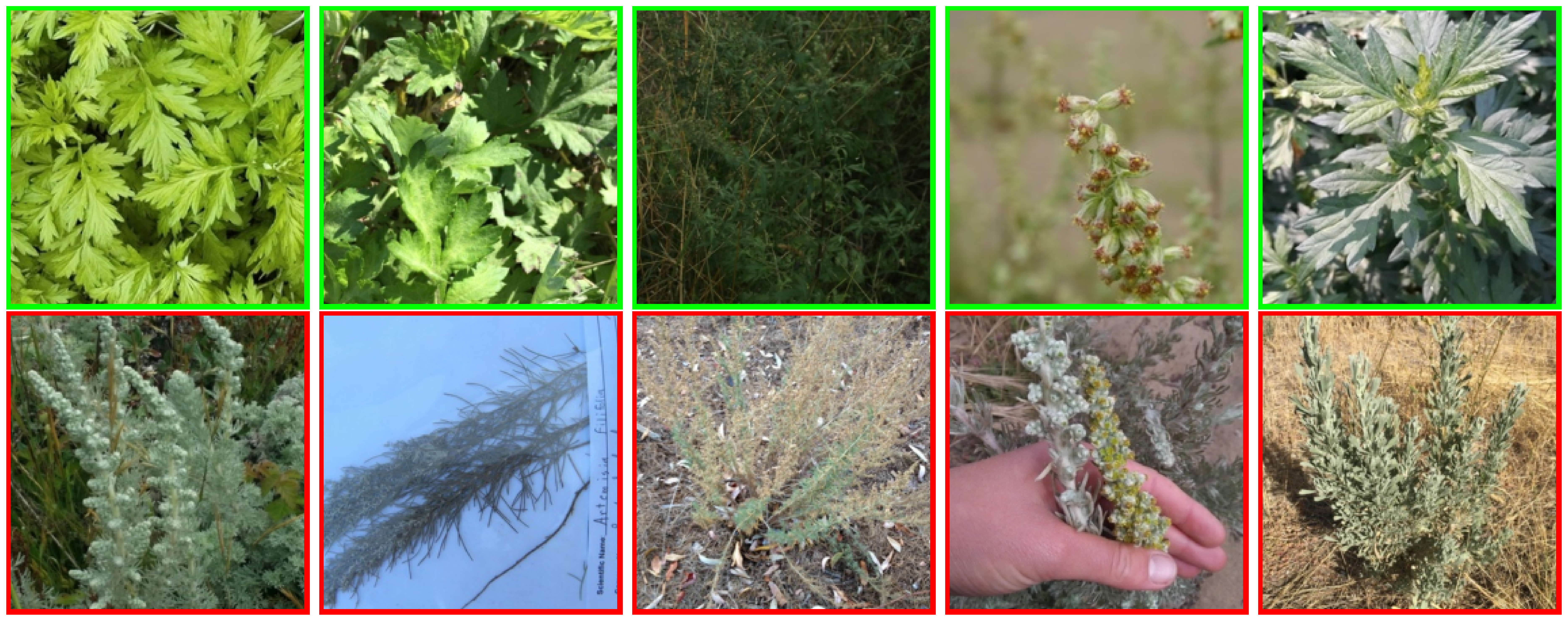
(a)

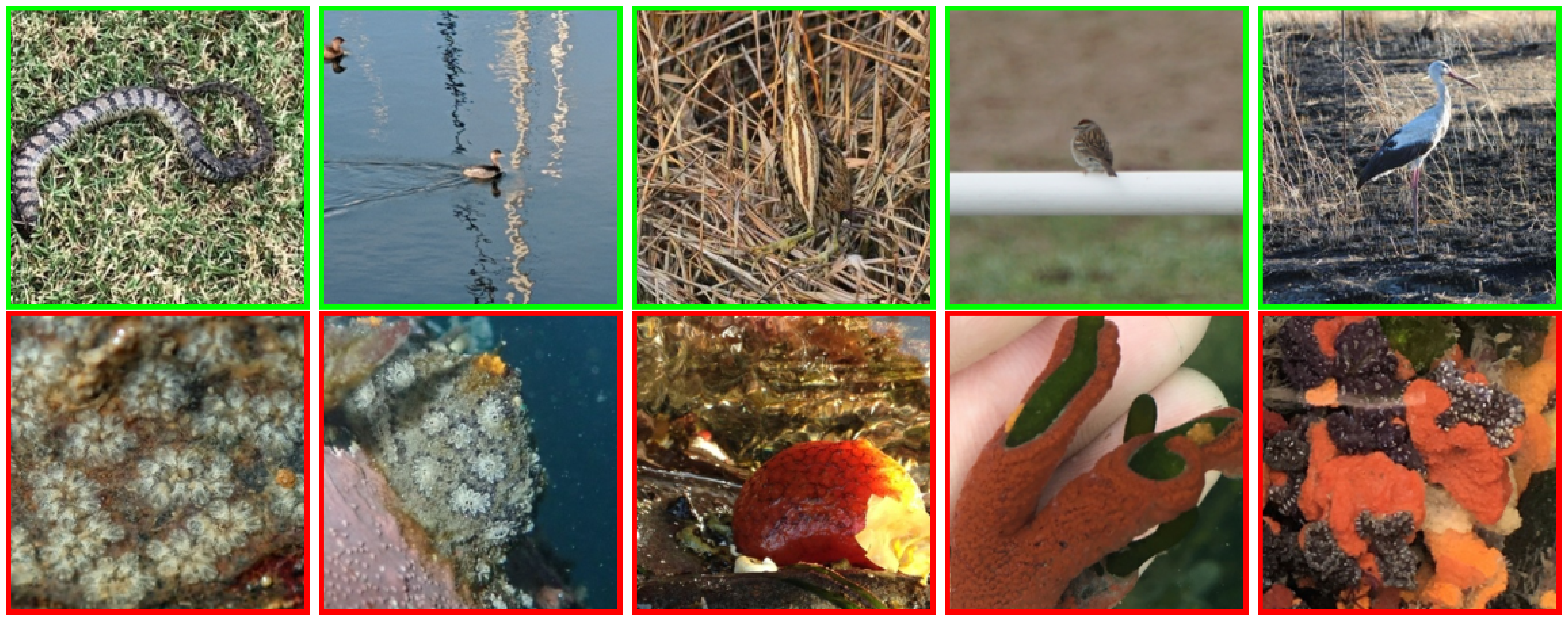
(b)

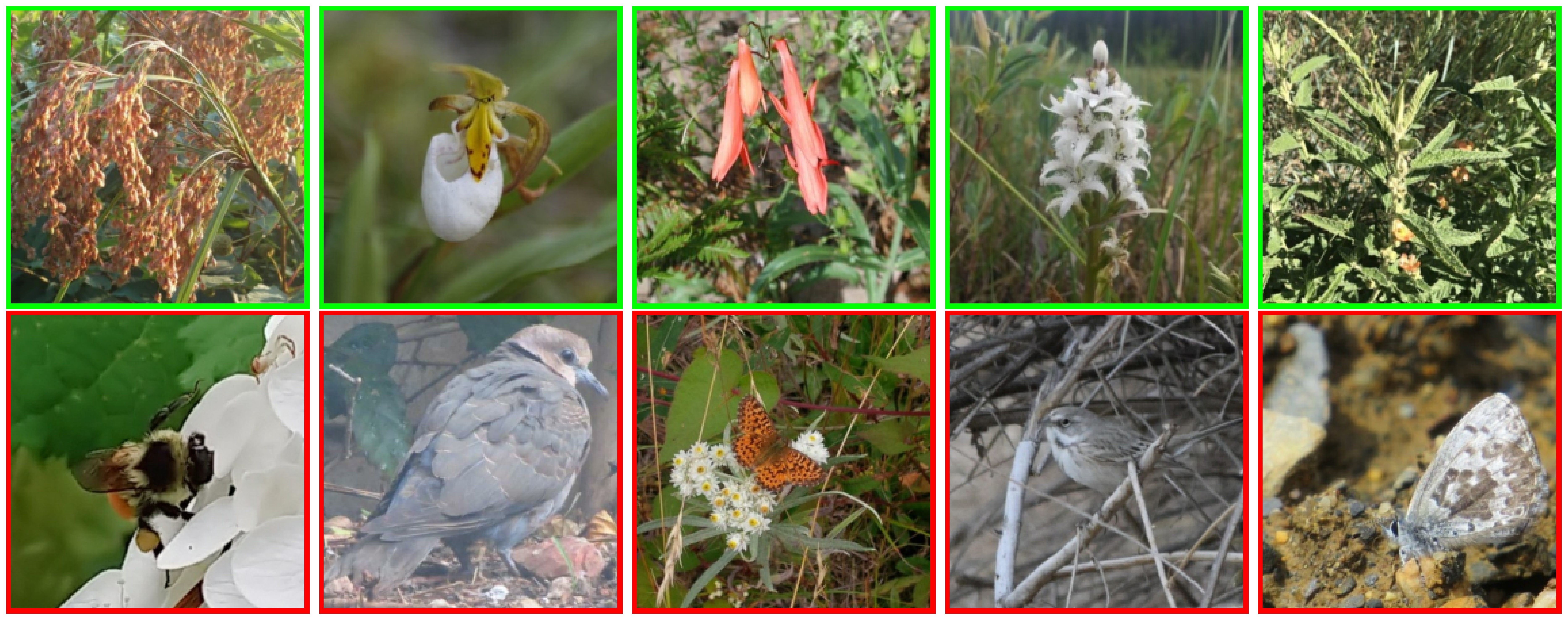
(c)

Figure 10: Examples of query samples from the proposed hierarchical sampling for iNaturalist. Positive query samples are highlighted in green while negative query samples are framed in red.

Appendix 0.B Usage of common names vs scientific names

Recall that in our experiments for iNaturalist, we have used common names instead of the official scientific names provided by the iNaturalist dataset. In this experiment, we rerun the comparison between our method and CLIPN using the scientific names and report the results in Table 4. Using the common names instead of the original scientific names significantly improves the performance across all methods. This is expected as CLIP has not been trained on scientific names which reduces its zero-shot capabilities [30].

Table 4: Comparison between common and scientific names on iNaturalist.

Backbone	Method	Common Names	Scientific Names
ViT-B-16 CLIP	CLIPN [43]	$\mathbf{41.95\pm 0.79}$	$35.56\pm 0.39$
	CLIPN [43]+FT	$\mathbf{50.77\pm 1.11}$	$45.78\pm 0.92$
	ANP+FT	$\mathbf{60.64\pm 1.02}$	$54.82\pm 1.06$
OpenCLIP	ANP+FT	$\mathbf{62.94\pm 1.11}$	$56.44\pm 1.27$

Appendix 0.C Quality of visually confusing classes

In this experiment, we investigate the quality of the confusing classes obtained using the Large Language Model. Instead of using visually confusing classes from the LLM, we use the existing groundtruth classes available in the original datasets. For each class label, we rank the other classes based on their cosine similarity to the target class and retain the 10 closest ones. For iNaturalist dataset, we restrict these classes to the neighbouring classes, i.e. the ones sharing a common ancestor with the target class. We keep the same methodology (ANP+FT) and only change the LLM based confusing classes with the groundtruth classes.

We report the results in Table 5 where we observe that our LLM based method is not far from the groundtruth based method. This hints that the LLM captures well visually confusing classes. With the noticeable exception of iNaturalist where the LLM performs better. The first possible explanation is that iNaturalist contains close concepts which can be better captured with the LLM. The second explanation is that the LLM generates common names for the visually confusing classes of iNaturalist which work better for CLIP.

Table 5: Groundtruth classes vs LLM prompts for negative prototypes, macro F1 score.

Method	iNat	SUN	Food	Textures	Pets	EuroSAT	Average
LLM	$\mathbf{60.32\pm 0.99}$	$94.19\pm 0.38$	${94.18\pm 0.20}$	${78.21\pm 0.88}$	${90.97\pm 0.88}$	$59.72\pm 0.98$	${79.60}$
Groundtruth	${55.69\pm 1.19}$	$\mathbf{97.56\pm 0.21}$	$\mathbf{97.72\pm 0.12}$	$\mathbf{88.59\pm 0.87}$	$\mathbf{96.23\pm 0.17}$	$\mathbf{76.95\pm 1.17}$	$\mathbf{85.46}$

Appendix 0.D Examples of visually confusing classes

In this section, we provide some examples for the visually confusing objects generated using the LLM. We highlight in blue classes that are present in the original dataset which were captured by the LLM. We observed on a large number of examples that the negative classes given by the LLM on EuroSAT and Textures often do not match existing classes in these two datasets which could explain the lower performance compared to other datasets.

• (iNat) Birds: Bats, Flying Squirrels, Butterflies, Moths, Dragonflies, Flying Fish, Flying Lemurs, Flying Frogs, Flying Snakes, Pterosaurs.

• (SUN) Abbey: Cathedral, Church, Monastery, Synagogue, Palace, Temple, Mosque, Castle, Mansion, Chapel.

• (Pets) Pug: French Bulldog, Boxer, Shih Tzu, Cavalier King Charles Spaniel, Boston Terrier, Bulldog, Bullmastiff, Staffordshire Bull Terrier, Lhasa Apso, Pekingese.

• (Food) Churros: French Fries, Spring Rolls, Donuts, Pretzels, Breadsticks, Cinnamon Sticks, Fries, Mozzarella Sticks, Cinnamon Rolls, Taquitos.

• (Textures) Bubbly: Pitted, Porous, Foamy, Frothy, Spongy, Puffy, Effervescent, Airy, Popcorn-like, Blisteblue.

• (Eurosat) River: Canal, Stream, Creek, Brook, Estuary, Fjord, Strait, Channel, Bayou, Inlet.

Appendix 0.E Accuracy and AUC scores

In this section, we report additional metrics for our main experiments. We first report the accuracy in Table 6. Note that for these experiments, the ratio of positive samples is $r=0.5$. Overall, we get similar results to the ones obtained using the macro F1-score.

Table 6: Accuracy score for multiple datasets.

Backbone	Method	iNat	SUN	Food	Textures	Pets	EuroSAT	Average
ViT-B-16 CLIP	CLIPN [43]	$54.44\pm 0.52$	$86.18\pm 0.43$	$72.96\pm 0.59$	$59.98\pm 0.46$	$76.12\pm 0.60$	$65.47\pm 0.61$	$69.19$
	CLIPN+FT (ours)	$58.41\pm 0.88$	$\mathbf{96.60\pm 0.16}$	$92.28\pm 0.29$	$77.85\pm 0.69$	$89.84\pm 0.47$	$\mathbf{74.64\pm 0.99}$	$81.60$
	ANP+FT (ours)	$\mathbf{65.31\pm 0.81}$	$94.43\pm 0.34$	$\mathbf{95.63\pm 0.17}$	$\mathbf{78.70\pm 0.93}$	$\mathbf{94.14\pm 0.62}$	$68.69\pm 0.75$	$\mathbf{82.81}$
ViT-B-32 CLIP	ZOC[10]	$60.24\pm 0.82$	$93.68\pm 0.31$	$92.56\pm 0.24$	$75.22\pm 0.59$	$88.75\pm 0.57$	$\mathbf{68.63\pm 0.91}$	$79.84$
	ZOC[10]+FT	$59.80\pm 0.86$	$\mathbf{95.34\pm 0.27}$	$92.70\pm 0.24$	$78.33\pm 0.62$	$88.73\pm 0.58$	$67.85\pm 0.84$	$80.46$
	ANP+FT (ours)	$\mathbf{64.61\pm 0.80}$	$94.29\pm 0.35$	$\mathbf{94.20\pm 0.20}$	$\mathbf{79.26\pm 0.74}$	$\mathbf{91.71\pm 0.71}$	${63.93\pm 0.79}$	$\mathbf{81.33}$
OpenCLIP	ANP+FT (ours)	$67.19\pm 0.90$	$96.90\pm 0.24$	$97.52\pm 0.12$	$87.55\pm 0.71$	$96.71\pm 0.20$	$77.23\pm 0.88$	$87.18$

Furthermore, we report in Table 7 the AUC score. Although being threshold invariant, the AUC reports shows how well the positive and negative samples are separated. The table shows that our method obtains on average competitive AUC scores. Our method outperforms alternatives on the iNaturalist dataaset where AUC scores are relatively low due to the difficulty of this setting. For other datasets, the different methods yield overall a good performance with an AUC score up to $99\%$ on SUN and Food. However, a high AUC score doesn’t translate directly to a good F1 score or accuracy as it is still important to select an appropriate threshold. Note that our main contribution is to propose a discriminative method which rejects the negative samples without a need of calibrating the threshold on validation samples drawn from the task.

Table 7: AUC score for multiple datasets.

Backbone	Method	iNat	SUN	Food	Textures	Pets	EuroSAT	Average
ViT-B-16 CLIP	CLIPN [43]	$65.77\pm 1.32$	$99.35\pm 0.06$	$98.80\pm 0.08$	$86.60\pm 0.82$	$98.11\pm 0.35$	$85.92\pm 0.79$	$89.09$
	CLIPN[43]+FT	$66.31\pm 1.38$	$\mathbf{99.47\pm 0.06}$	$99.07\pm 0.07$	$\mathbf{88.96\pm 0.78}$	$\mathbf{98.66\pm 0.26}$	$\mathbf{86.20\pm 0.76}$	$\mathbf{89.78}$
	ANP+FT (ours)	$\mathbf{73.41\pm 1.12}$	$98.93\pm 0.15$	$\mathbf{99.17\pm 0.07}$	$85.46\pm 1.19$	$95.52\pm 1.10$	$83.36\pm 0.63$	$89.31$
ViT-B-32 CLIP	ZOC[10]	$69.28\pm 1.10$	$\mathbf{99.21\pm 0.10}$	$\mathbf{99.08\pm 0.06}$	$\mathbf{90.32\pm 0.57}$	$97.37\pm 0.60$	$79.16\pm 0.89$	$\mathbf{89.07}$
	ZOC[10]+FT	$68.69\pm 1.15$	$99.20\pm 0.10$	$99.07\pm 0.06$	$89.42\pm 0.61$	$\mathbf{97.43\pm 0.55}$	$\mathbf{79.72\pm 0.85}$	$88.92$
	ANP+FT (ours)	$\mathbf{71.35\pm 1.10}$	$98.76\pm 0.20$	$98.76\pm 0.08$	${86.56\pm 0.96}$	$94.29\pm 1.19$	${79.44\pm 0.83}$	${88.19}$
OpenCLIP	ANP+FT (ours)	$74.41\pm 1.25$	$99.55\pm 0.09$	$99.60\pm 0.04$	$94.73\pm 0.51$	$99.86\pm 0.02$	$86.74\pm 0.74$	$92.48$

Appendix 0.F Threshold transfer

In this section, we investigate the choice of the fixed threshold and its transferability from one dataset to another. Firstly, we compare two methods for selecting the fixed threshold on ImageNet1K: 1. By performing a hyperparameter search over a range of values and selecting the one which maximizes the F1 score over $1000$ tasks sampled from ImageNet1K. 2. By selecting the optimal threshold per task and averaging these values. Our results in Table 8 for the Fixed Threshold (FT) method show that it is better to use the average of optimal thresholds.

Table 8: Average macro F1 score for multiple datasets. Comparison for selecting the threshold from ImageNet1K.

Selection criteria	iNat	SUN	Food	Textures	Pets	EuroSAT	Average
Hyperparameter search	$54.70\pm 1.18$	$96.63\pm 0.20$	$95.41\pm 0.21$	$82.42\pm 0.67$	$84.16\pm 0.38$	$\mathbf{75.82\pm 0.97}$	$81.53$
Average of optimal thresholds	$\mathbf{56.60\pm 1.25}$	$\mathbf{97.36\pm 0.21}$	$\mathbf{97.49\pm 0.13}$	$\mathbf{86.62\pm 0.71}$	$\mathbf{91.56\pm 0.27}$	$72.48\pm 1.07$	$\mathbf{83.68}$

Secondly, we investigate the transferability of the threshold from one dataset to another. We estimate the best threshold from a source dataset using the average of optimal thresholds, then we evaluate its performance on the remaining datasets. We report the performance of the Fixed Threshold (FT) method in Figure 11. The Figure shows that the threshold from ImageNet1K achieves the best results on average and is overall well performing across the different datasets.

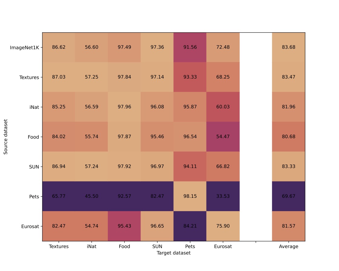
Figure 11: Macro F1 score when transferring a threshold from a source dataset to a target dataset.

References

- [1] Achiam, J., Adler, S., Agarwal, S., Ahmad, L., Akkaya, I., Aleman, F.L., Almeida, D., Altenschmidt, J., Altman, S., Anadkat, S., et al.: Gpt-4 technical report. arXiv preprint arXiv:2303.08774 (2023)
- [2] Bossard, L., Guillaumin, M., Van Gool, L.: Food-101–mining discriminative components with random forests. In: Computer Vision–ECCV 2014: 13th European Conference, Zurich, Switzerland, September 6-12, 2014, Proceedings, Part VI 13. pp. 446–461. Springer (2014)
- [3] Boudiaf, M., Bennequin, E., Tami, M., Toubhans, A., Piantanida, P., Hudelot, C., Ben Ayed, I.: Open-set likelihood maximization for few-shot learning. In: Proceedings of the IEEE/CVF Conference on Computer Vision and Pattern Recognition. pp. 24007–24016 (2023)
- [4] Chen, X., Konukoglu, E.: Unsupervised detection of lesions in brain mri using constrained adversarial auto-encoders. arXiv preprint arXiv:1806.04972 (2018)
- [5] Chen, Y., Zhou, X.S., Huang, T.S.: One-class svm for learning in image retrieval. In: Proceedings 2001 international conference on image processing (Cat. No. 01CH37205). vol. 1, pp. 34–37. IEEE (2001)
- [6] Cheng, C., Song, L., Xue, R., Wang, H., Sun, H., Ge, Y., Shan, Y.: Meta-adapter: An online few-shot learner for vision-language model. arXiv preprint arXiv:2311.03774 (2023)
- [7] Cherti, M., Beaumont, R., Wightman, R., Wortsman, M., Ilharco, G., Gordon, C., Schuhmann, C., Schmidt, L., Jitsev, J.: Reproducible scaling laws for contrastive language-image learning. In: Proceedings of the IEEE/CVF Conference on Computer Vision and Pattern Recognition. pp. 2818–2829 (2023)
- [8] Cimpoi, M., Maji, S., Kokkinos, I., Mohamed, S., Vedaldi, A.: Describing textures in the wild. In: Proceedings of the IEEE conference on computer vision and pattern recognition. pp. 3606–3613 (2014)
- [9] Deecke, L., Vandermeulen, R., Ruff, L., Mandt, S., Kloft, M.: Image anomaly detection with generative adversarial networks. In: Machine Learning and Knowledge Discovery in Databases: European Conference, ECML PKDD 2018, Dublin, Ireland, September 10–14, 2018, Proceedings, Part I 18. pp. 3–17. Springer (2019)
- [10] Esmaeilpour, S., Liu, B., Robertson, E., Shu, L.: Zero-shot out-of-distribution detection based on the pre-trained model clip. In: Proceedings of the AAAI conference on artificial intelligence. vol. 36, pp. 6568–6576 (2022)
- [11] Görnitz, N., Kloft, M., Rieck, K., Brefeld, U.: Toward supervised anomaly detection. Journal of Artificial Intelligence Research 46, 235–262 (2013)
- [12] Goyal, S., Raghunathan, A., Jain, M., Simhadri, H.V., Jain, P.: Drocc: Deep robust one-class classification. In: International conference on machine learning. pp. 3711–3721. PMLR (2020)
- [13] Helber, P., Bischke, B., Dengel, A., Borth, D.: Eurosat: A novel dataset and deep learning benchmark for land use and land cover classification. IEEE Journal of Selected Topics in Applied Earth Observations and Remote Sensing 12(7), 2217–2226 (2019)
- [14] Hendrycks, D., Basart, S., Mazeika, M., Zou, A., Kwon, J., Mostajabi, M., Steinhardt, J., Song, D.: Scaling out-of-distribution detection for real-world settings. arXiv preprint arXiv:1911.11132 (2019)
- [15] Hendrycks, D., Gimpel, K.: A baseline for detecting misclassified and out-of-distribution examples in neural networks. arXiv preprint arXiv:1610.02136 (2016)
- [16] Huang, S., Ma, J., Han, G., Chang, S.F.: Task-adaptive negative envision for few-shot open-set recognition. In: Proceedings of the IEEE/CVF Conference on Computer Vision and Pattern Recognition. pp. 7171–7180 (2022)
- [17] Jeong, M., Choi, S., Kim, C.: Few-shot open-set recognition by transformation consistency. In: Proceedings of the IEEE/CVF Conference on Computer Vision and Pattern Recognition. pp. 12566–12575 (2021)
- [18] Jia, C., Yang, Y., Xia, Y., Chen, Y.T., Parekh, Z., Pham, H., Le, Q., Sung, Y.H., Li, Z., Duerig, T.: Scaling up visual and vision-language representation learning with noisy text supervision. In: International conference on machine learning. pp. 4904–4916. PMLR (2021)
- [19] Kim, K.H., Shim, S., Lim, Y., Jeon, J., Choi, J., Kim, B., Yoon, A.S.: Rapp: Novelty detection with reconstruction along projection pathway. In: International Conference on Learning Representations (2019)
- [20] Lee, K., Lee, H., Lee, K., Shin, J.: Training confidence-calibrated classifiers for detecting out-of-distribution samples. arXiv preprint arXiv:1711.09325 (2017)
- [21] Liang, S., Li, Y., Srikant, R.: Enhancing the reliability of out-of-distribution image detection in neural networks. arXiv preprint arXiv:1706.02690 (2017)
- [22] Liang, V.W., Zhang, Y., Kwon, Y., Yeung, S., Zou, J.Y.: Mind the gap: Understanding the modality gap in multi-modal contrastive representation learning. Advances in Neural Information Processing Systems 35, 17612–17625 (2022)
- [23] Lin, T.Y., Maire, M., Belongie, S., Hays, J., Perona, P., Ramanan, D., Dollár, P., Zitnick, C.L.: Microsoft coco: Common objects in context. In: Computer Vision–ECCV 2014: 13th European Conference, Zurich, Switzerland, September 6-12, 2014, Proceedings, Part V 13. pp. 740–755. Springer (2014)
- [24] Lin, Z., Yu, S., Kuang, Z., Pathak, D., Ramanan, D.: Multimodality helps unimodality: Cross-modal few-shot learning with multimodal models. In: Proceedings of the IEEE/CVF Conference on Computer Vision and Pattern Recognition. pp. 19325–19337 (2023)
- [25] Liu, B., Kang, H., Li, H., Hua, G., Vasconcelos, N.: Few-shot open-set recognition using meta-learning. In: Proceedings of the IEEE/CVF Conference on Computer Vision and Pattern Recognition. pp. 8798–8807 (2020)
- [26] Liu, W., Wang, X., Owens, J., Li, Y.: Energy-based out-of-distribution detection. Advances in neural information processing systems 33, 21464–21475 (2020)
- [27] Ming, Y., Cai, Z., Gu, J., Sun, Y., Li, W., Li, Y.: Delving into out-of-distribution detection with vision-language representations. Advances in Neural Information Processing Systems 35, 35087–35102 (2022)
- [28] Miyai, A., Yu, Q., Irie, G., Aizawa, K.: Locoop: Few-shot out-of-distribution detection via prompt learning. arXiv preprint arXiv:2306.01293 (2023)
- [29] Pang, G., Shen, C., Jin, H., van den Hengel, A.: Deep weakly-supervised anomaly detection. In: Proceedings of the 29th ACM SIGKDD Conference on Knowledge Discovery and Data Mining. pp. 1795–1807 (2023)
- [30] Parashar, S., Lin, Z., Li, Y., Kong, S.: Prompting scientific names for zero-shot species recognition. arXiv preprint arXiv:2310.09929 (2023)
- [31] Parkhi, O.M., Vedaldi, A., Zisserman, A., Jawahar, C.: Cats and dogs. In: 2012 IEEE conference on computer vision and pattern recognition. pp. 3498–3505. IEEE (2012)
- [32] Principi, E., Vesperini, F., Squartini, S., Piazza, F.: Acoustic novelty detection with adversarial autoencoders. In: 2017 International Joint Conference on Neural Networks (IJCNN). pp. 3324–3330. IEEE (2017)
- [33] Radford, A., Kim, J.W., Hallacy, C., Ramesh, A., Goh, G., Agarwal, S., Sastry, G., Askell, A., Mishkin, P., Clark, J., et al.: Learning transferable visual models from natural language supervision. In: International conference on machine learning. pp. 8748–8763. PMLR (2021)
- [34] Ruff, L., Kauffmann, J.R., Vandermeulen, R.A., Montavon, G., Samek, W., Kloft, M., Dietterich, T.G., Müller, K.R.: A unifying review of deep and shallow anomaly detection. Proceedings of the IEEE 109(5), 756–795 (2021)
- [35] Ruff, L., Vandermeulen, R., Goernitz, N., Deecke, L., Siddiqui, S.A., Binder, A., Müller, E., Kloft, M.: Deep one-class classification. In: International conference on machine learning. pp. 4393–4402. PMLR (2018)
- [36] Ruff, L., Vandermeulen, R.A., Görnitz, N., Binder, A., Müller, E., Müller, K.R., Kloft, M.: Deep semi-supervised anomaly detection. arXiv preprint arXiv:1906.02694 (2019)
- [37] Sabokrou, M., Khalooei, M., Fathy, M., Adeli, E.: Adversarially learned one-class classifier for novelty detection. In: Proceedings of the IEEE conference on computer vision and pattern recognition. pp. 3379–3388 (2018)
- [38] Scheirer, W.J., de Rezende Rocha, A., Sapkota, A., Boult, T.E.: Toward open set recognition. IEEE transactions on pattern analysis and machine intelligence 35(7), 1757–1772 (2012)
- [39] Schlachter, P., Liao, Y., Yang, B.: Open-set recognition using intra-class splitting. In: 2019 27th European signal processing conference (EUSIPCO). pp. 1–5. IEEE (2019)
- [40] Schlegl, T., Seeböck, P., Waldstein, S.M., Schmidt-Erfurth, U., Langs, G.: Unsupervised anomaly detection with generative adversarial networks to guide marker discovery. In: International conference on information processing in medical imaging. pp. 146–157. Springer (2017)
- [41] Silva-Rodriguez, J., Hajimiri, S., Ayed, I.B., Dolz, J.: A closer look at the few-shot adaptation of large vision-language models. arXiv preprint arXiv:2312.12730 (2023)
- [42] Van Horn, G., Mac Aodha, O., Song, Y., Cui, Y., Sun, C., Shepard, A., Adam, H., Perona, P., Belongie, S.: The inaturalist species classification and detection dataset. In: Proceedings of the IEEE conference on computer vision and pattern recognition. pp. 8769–8778 (2018)
- [43] Wang, H., Li, Y., Yao, H., Li, X.: Clipn for zero-shot ood detection: Teaching clip to say no. In: Proceedings of the IEEE/CVF International Conference on Computer Vision. pp. 1802–1812 (2023)
- [44] Wang, X., Ye, Y., Gupta, A.: Zero-shot recognition via semantic embeddings and knowledge graphs. In: Proceedings of the IEEE conference on computer vision and pattern recognition. pp. 6857–6866 (2018)
- [45] Xiao, J., Hays, J., Ehinger, K.A., Oliva, A., Torralba, A.: Sun database: Large-scale scene recognition from abbey to zoo. In: 2010 IEEE computer society conference on computer vision and pattern recognition. pp. 3485–3492. IEEE (2010)
- [46] Zhang, Z., Xiang, X.: Decoupling maxlogit for out-of-distribution detection. In: Proceedings of the IEEE/CVF Conference on Computer Vision and Pattern Recognition. pp. 3388–3397 (2023)
- [47] Zhou, D.W., Ye, H.J., Zhan, D.C.: Learning placeholders for open-set recognition. In: Proceedings of the IEEE/CVF conference on computer vision and pattern recognition. pp. 4401–4410 (2021)
- [48] Zhou, K., Yang, J., Loy, C.C., Liu, Z.: Learning to prompt for vision-language models. International Journal of Computer Vision 130(9), 2337–2348 (2022)