Metin Gürses
Department of Mathematics, Faculty of Science
Bilkent University, 06800 Ankara - Turkey
Aslı Pekcan
Department of Mathematics, Faculty of Science Hacettepe University, 06800 Ankara - Turkeygurses@fen.bilkent.edu.trEmail:aslipekcan@hacettepe.edu.tr
Abstract
To obtain new integrable nonlinear differential equations there are some well-known methods such as Lax equations with different Lax representations. There are also some other methods which are based on integrable scalar nonlinear partial differential equations. We show that some systems of integrable equations published recently are the -extension of integrable scalar equations. For illustration we give Korteweg-de Vries, Kaup-Kupershmidt, and Sawada-Kotera equations as examples. By the use of such an extension of integrable scalar equations we obtain some new integrable systems with recursion operators. We give also the soliton solutions of the system equations and integrable standard nonlocal and shifted nonlocal reductions of these systems.
There are many ways of obtaining new integrable systems of equations such as taking the Lax representations in algebras of higher rank. In these methods we obtain real and complex valued coupled nonlinear equations which possess recursion operators and Hirota bilinear forms. There are also some other methods which use integrable systems with less number of dynamical variables to produce integrable systems with more dynamical variables.
Recently we observe such an effort to obtain systems of Sawada-Kotera (SK) and Kaup-Kuperschmidt (KK) equations [1], [2] by the use of Lax representations. The purpose of this paper is to show that the systems obtained in [1], [2] are easily obtained by a method that we call -extensions of the SK and KK equations. This method is so general that it can be used to any integrable scalar equation.
Let be a special subclass of matrices. Let and be given by where and are independent components of the matrix , is the identity matrix, and
(1.1)
where is a real constant. Since , products of all such matrices are also in this subclass of matrices. Hence is a commutative subclass of matrices. Due to the special properties of this subclass of matrices we can generate new systems of integrable equations from scalar integrable equations. We call this method as -extension of integrable scalar equations. As an illustration consider the well-known Korteweg-de Vries (KdV) equation with Lax pair , so that the Lax equation is satisfied by virtue of the KdV equation
(1.2)
and the recursion operator [3]. Here is the total -derivative and is the standard
anti-derivative. Then -extension of the KdV equation, its Lax pair, and recursion operator are respectively given as
(1.3)
(1.4)
(1.5)
(1.6)
where
(1.7)
The pair and solves the Lax equation due to the -extension of the KdV equation (1.3) for . In componentwise the above equations give a system of equations for the dynamical variables and
(1.8)
(1.9)
admitting the recursion operator
(1.10)
It is interesting that the above extension of the KdV equation is equivalent to the (pseudo)-complexification of the KdV equation. First let where . Then scale (for ) so the above system becomes
(1.11)
(1.12)
Remark 1. For the above system is the extension of the KdV with its linearized equation for . For this system is a consequence of the (pseudo)-complexification of the KdV equation where is the pseudo-complex unit .
For complex numbers but for pseudo-complex numbers . Complex conjugation for both cases is the same . Hence our conclusion is that
-extension of the KdV equation is the unification of linearization and pseudo-complexification of the KdV equation. Our second conclusion is that this is valid in general.
We use -extension method to integrable scalar equations to obtain systems of integrable equations and to obtain new integrable nonlocal equations. This method consists of three main steps. The first step is to replace the dynamical variable of the integrable scalar equation by where and are the dynamical variables of the system. Here, since the system of equations contain also the constant . We write the dynamical equations for and . By using the recursion operator of the scalar equation we obtain the recursion operator of the system equations for and . Furthermore, if the Hirota bilinear form of the scalar equation is known then we obtain the bilinear form of the system of equations. At this step we obtain an integrable system of equations for and . Second step is to obtain the symmetrical version of the system equations by defining new dynamical variables and . At the same time one can obtain the recursion operator with respect to the dynamical variables and . The third step is to apply consistent reductions; standard (unshifted) nonlocal reductions and , and shifted nonlocal reductions for and for where to obtain standard nonlocal and shifted nonlocal reductions of the system for and [4]-[15]. Using the reduction formulas, we can obtain the recursion operators of the nonlocal differential equations. In general these equations will be new and integrable. Soliton solutions of the standard nonlocal and shifted nonlocal equations can be easily obtained by using soliton solutions of the systems and reduction formulas.
In the following section we find extensions of the SK and KK equations, their recursion operators, and symmetrical versions of these systems. In Section 3 we obtain nonlocal reductions of the SK and KK systems. In Section 4 we find shifted nonlocal reductions of SK and KK sytems. In Section 5 we present Hirota bilinearization of SK and KK systems and give one-soliton solutions of the equations.
2 SK and KK systems
Recently, we observe some publications on the extensions of higher order integrable equations by using the Lax representations [1], [2]. Here we show that such extensions are nothing but the -extension of an integrable scalar equation explained in the previous section.
Scalar versions of SK and KK equations are given respectively as [1], [2], [16]-[20]:
(1) SK equation, Lax pair, and recursion operator
(2.1)
(2.2)
(2.3)
(2.4)
(2) KK equation, Lax pair, and recursion operator
(2.5)
(2.6)
(2.7)
(2.8)
-extensions of these equations, Lax pairs, and recursion operators are respectively given as
(3) SK system, Lax pair, and recursion operator
(2.9)
(2.10)
(2.11)
(2.12)
The above equations correspond to the system of equations for the dynamical variables and as
(2.13)
(2.14)
The recursion operator of this system is
(2.15)
where
(2.16)
(2.17)
By letting , , and , where is a constant, we get symmetrical version of the system (2.13) and (2.14) as
(2.18)
(2.19)
(4) KK system, Lax pair, and recursion operator
(2.20)
(2.21)
(2.22)
(2.23)
In componentwise the above equations give the following system of equations for the dynamical variables and
(2.24)
(2.25)
The recursion operator of the above system is
(2.26)
where
(2.27)
(2.28)
Letting , , and , where is a constant, yields symmetrical version of the system (2.24) and (2.25) as
(2.29)
(2.30)
We use the symmetrical versions of systems to obtain nonlocal reductions of them which will be the subject of the next section.
3 Nonlocal reductions
In the last decade there has been intensive interest to obtain new integrable nonlocal equations [4]-[9]. Here we give some new nonlocal equations of fifth order, namely nonlocal SK and nonlocal KK equations.
The above symmetrical versions of SK (2.18), (2.19), and KK (2.29), (2.30) systems are good candidates to obtain new nonlocal integrable equations of fifth order.
(1) Nonlocal SK equations:
Consider the symmetrical SK system (2.18) and (2.19).
(a) , .
When we apply this real nonlocal reduction on the SK system (2.18) and (2.19) we get the condition for consistency.
Therefore here we have only one nonlocal reduction which reduces the system (2.18), (2.19) to the following nonlocal
space-time reversal SK equation
(3.1)
where .
(b) , .
Applying the complex nonlocal reduction to the symmetrical SK system (2.18) and (2.19) yields the constraint
(3.2)
for consistency. The system (2.18), (2.19) reduces to nonlocal space reversal SK equation for with ; nonlocal time reversal SK equation for with ; nonlocal space-time reversal equation SK for with
given by
(3.3)
where , . Hence the above equation consists of three different reductions representing different nonlocal complex SK equations.
(2) Nonlocal KK equations:
Consider the symmetrical KK system (2.24) and (2.25).
(a) , .
Similar to the symmetrical SK system, applying the reduction to the symmetrical KK system (2.24) and (2.25)
gives the constraint for consistency. Hence we have only one real nonlocal reduction which reduces the system (2.29) and (2.30) to the nonlocal
space-time reversal KK equation
(3.4)
where .
(b) , .
When we apply this complex nonlocal reduction to the symmetrical KK system (2.29) and (2.30) we obtain the condition
for consistency as in the SK system case. The KK system (2.29), (2.30) reduces to nonlocal space reversal KK equation for with ; nonlocal time reversal KK equation for with ; nonlocal space-time reversal KK equation for with . Explicitly, we have
(3.5)
where , . Then the above equation consists of three different reductions representing different nonlocal complex KK equations.
By using the reduction formulas (1).a, (1).b, (2).a, and (2).b, and the recursion operators of SK and KK systems we can obtain the recursions operators (2.15) and (2.26) of the nonlocal SK and nonlocal KK equations, respectively.
4 Shifted nonlocal reductions
After quite a few works on integrable nonlocal reductions, Ablowitz and Musslimani generalized standard nonlocal reductions to shifted nonlocal reductions in [10] as
(4.1)
for . It is obvious that if , the shifted reductions become standard (unshifted) nonlocal reductions. There are also several works on integrable shifted nonlocal equations and their different type of solutions obtained by various type of methods [11]-[15].
Here we give shifted nonlocal SK and KK equations by applying the above shifted nonlocal reductions to the symmetrical SK system (2.18), (2.19), and the
symmetrical KK system (2.29), (2.30).
(1) Shifted nonlocal SK equations:
(a) , , .
Using this real shifted nonlocal reduction on the SK system (2.18), (2.19) requires the condition to be satisfied for consistency.
Hence we have only one shifted nonlocal reduction and the corresponding shifted nonlocal
space-time reversal SK equation is
(4.2)
where , .
(b) , .
Applying the complex shifted nonlocal reduction to the system (2.18), (2.19) gives the following constraint
(4.3)
for consistency. Therefore the symmetrical SK system reduces to shifted nonlocal SK equations represented by
(4.4)
where , , . The above equation consists three shifted nonlocal SK equations; shifted nonlocal space reversal SK equation for , , shifted nonlocal time reversal SK equation for , , and shifted nonlocal space-time reversal equation SK equation for , .
(2) Shifted nonlocal KK equations:
(a) , , .
Applying the reduction to the system (2.24) and (2.25)
yields the condition for consistency. Similar to the SK system case, we have only one real shifted nonlocal reduction reducing the KK system (2.29) and (2.30) to the shifted nonlocal
space-time reversal KK equation
(4.5)
where , .
(b) , , .
Under the complex shifted nonlocal reduction we get the condition for consistency and the symmetrical KK system (2.29), (2.30) reduces to three different shifted nonlocal KK equations given by
(4.6)
where , , . Indeed we have shifted nonlocal space reversal KK equation for , , shifted nonlocal time reversal KK equation for , , and shifted nonlocal space-time reversal KK equation for , .
5 Hirota bilinearization and one-soliton solution
It is also possible to write the Hirota bilinear forms of the extended equations. Starting with the Hirota bilinear forms of the scalar SK and KK equations and writing them for extended variable we obtain the corresponding Hirota forms of SK and KK systems.
Let then the Hirota bilinear form of SK equation is given as [21], [22], [23]
(5.1)
For the system of equations we make use of the above bilinearization. We let where and . Here and are the functions to be determined by the Hirota method. Then we get
(5.2)
or equivalently
(5.3)
When we write the above equation in componentwise we obtain
(5.4)
(5.5)
Hence solving and from the above expressions and using them in , we obtain and in terms of and . To find one-soliton solution of the system (2.13), (2.14), take and for some constants , and , . Inserting this choice into the Hirota bilinear form (5.4) and (5.5) yields
(5.6)
and
(5.7)
where
(5.8)
(5.9)
(5.10)
where .
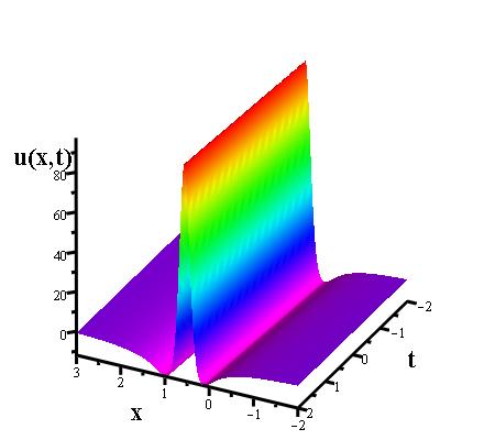
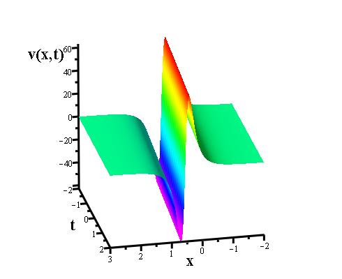
Example 1. Take particular values for the parameters of the solution (5.7) as , , . Then the solution becomes
(5.11)
The graphs of the above solutions are given in Figure 1.
Figure 1: One-soliton solution of the SK system (2.13), (2.14) for , , , .
Letting yields the Hirota bilinear form of KK equation as [21], [24], [25]
(5.12)
(5.13)
where is an auxiliary function. Similar to the SK system, we let where . We determine and by the Hirota method. We get
(5.14)
(5.15)
which is equivalent to
(5.16)
(5.17)
where . In componentwise we have
(5.18)
(5.19)
(5.20)
(5.21)
To obtain one-soliton solution of the system (2.24), (2.25) we take , , , and , where for some constants , and , . From the above system we get and the following constraints:
(5.22)
Hence one-soliton solution of the KK system (2.24), (2.25) is given by the pair
(5.23)
where
(5.24)
(5.25)
(5.26)
where .
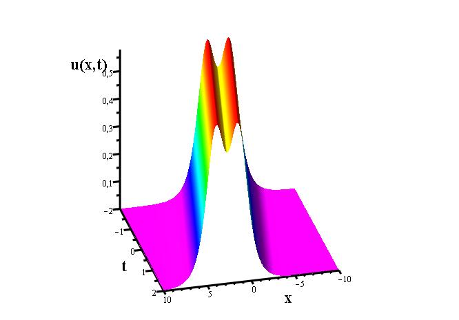
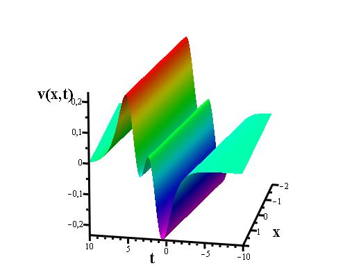
Example 2. Consider the particular values for the parameters of the solution (5.23) as , . We have the solution where
(5.27)
(5.28)
The graphs of the above solutions are given in Figure 2.
Figure 2: One-soliton solution of the KK system (2.24), (2.25) for , .
Remark 2. We note that taking different expansions for the functions and in (5.4)
and (5.5) or in (5.18)-(5.21) may put strong conditions on the parameters
yielding or . For instance, if we use , , where , are constants, in
the Hirota bilinear form (5.4), (5.5) we get and also making . In this case the SK system (2.13), (2.14)
for the dynamical variables and reduces to the SK equation (2.1) for .
Since the expressions are quite longer we shall not display two- and three-soliton solutions of the SK and KK systems here. The more interesting case is the soliton solutions of the nonlocal SK and KK equations presented in Section 3. They can be easily obtained by using the above soliton solutions of the systems with the reduction formulas (1).a, (1).b, (2).a, and (2).b presented in Section 3. These equations will restrict parameters in the soliton solutions (5.7) and (5.23).
We shall discuss two- and three-soliton solutions of the SK and KK systems and soliton solutions of the nonlocal SK and KK equations in a forthcoming publication.
6 Concluding remarks
In this work we obtained systems of integrable equations with their recursion operators from scalar integrable equations by applying -extension. We used this method for SK and KK equations and obtained SK system and KK system of equations, respectively. Applying the nonlocal reductions to the symmetric versions of SK and KK systems we obtained eight different new standard nonlocal and eight different new shifted nonlocal integrable differential equations. We presented also one-soliton solutions of the SK and KK systems.
7 Acknowledgment
This work is partially supported by the Scientific
and Technological Research Council of Turkey (TÜBİTAK).
References
[1] Z. Qi-Liang, J. Man, and L. Sen-Yue, Fifth-order Alice-Bob systems and their
abundant periodic and solitary wave solutions, Commun. Theor. Phys. 71, 1149 (2019).
[2] Z. Qi-Liang, L. Sen-Yue, and J. Man, Solitons and soliton molecules in two nonlocal Alice-Bob Sawada-Kotera system, Commun. Theor. Phys. 72, 060005 (2020).
[3] C.S. Gardner, J.M. Greene, M.D. Kruskal, and R.M. Miura, Korteweg-de Vries equation and generalizations. VI. Methods for exact solution, Commun. Pure Appl. Math.
27, 97–133 )1974.
[4] M.J. Ablowitz and Z.H. Musslimani, Integrable nonlocal nonlinear Schrödinger equation Phys. Rev. Lett. 110, 064105 (2013).
[5] M.J. Ablowitz and Z.H. Musslimani, Inverse scattering transform for the integrable nonlocal nonlinear Schrödinger equation, Nonlinearity 29, 915–946 (2016).
[7] M. Gürses and A. Pekcan, Nonlocal nonlinear Schrödinger equations and their soliton solutions, J. Math. Phys. 59, 051501, (2018).
[8] M. Gürses and A. Pekcan, Integrable Nonlocal Reductions, ”Symmetries, Differential Equations and Applications SDEA-III, Istanbul, Turkey, August 2017”, Editors: V.G. Kac, P.J. Olver, P. Winternitz, and T. Ozer, Springer Proceedings in Mathematics and Statistics, 266, (2018).
[9] M. Gürses and A. Pekcan, Nonlocal nonlinear modified KdV equations and their soliton solutions,
Commun. Nonlinear Sci. Numer. Simulat. 67, 427–448 (2019).
[10] M.J. Ablowitz and Z.H. Musslimani, Integrable space-time shifted nonlocal nonlinear equations, Phys. Lett. A 409, 127516, (2021).
[11] M.J. Ablowitz, Z.H. Musslimani, and N.J. Ossi, Inverse scattering transform for continuous and discrete space-time shifted integrable equations, arXiv:2312.11780v2 [nlin.SI].
[12] M. Gürses and A. Pekcan, Soliton solutions of the shifted nonlocal NLS and MKdV equations, Phys. Lett. A 422, 127793 (2022).
[13] S.M. Liu, J. Wang, and D.J. Zhang, Solutions to integrable space-time shifted nonlocal equations, Rep. Math. Phys. 89(2), 199–220 (2022).
[14] X. Wang and J. Wei, Three types of Darboux transformation and general soliton solutions for the space-shifted nonlocal PT symmetric nonlinear Schrödinger equation, Appl. Math. Lett. 130, 107998 (2022).
[15] X.B. Wang and S.F. Tian, Exotic localized waves in the shifted nonlocal multicomponent nonlinear Schrödinger equation, Theor. Math. Phys. 212, 1193–1210, (2022).
[16] M. Gürses, A. Karasu, and V. Sokolov, On construction of recursion operators from Lax
representation, J. Math. Phys. 40, 6473–6490 (1999).
[17] J.P. Wang, A list of dimensional integrable equations and their properties, J. Nonlinear Math. Phys. 9, 213–233 (2002).
[18] M. Euler and N. Euler, A class of semilinear fifth-order evolution equations: Recursion
operators and multi potentialisations, J. Nonlinear Math. Phys. 18, 61–75 (2011).
[19] C.T. Lee and C.C. Lee, Lax pairs and Hamiltonians for the Kaup–Kupershmidt-type equation, Phys. Scr. 85, 035004 (2012).
[20] J.D. Kaup, On the inverse scattering problem for cubic-eigenvalue problems of the class , Stud. Appl. Math. 62, 189–216 (1980).
[21] M. Jimbo and T. Miwa, Solitons and infinite dimensional Lie algebras, Publ. RIMS, Kyotu Univ. 19, 943 (1983).
[22] A.K.M. Kazi Sazzad Hossain and M. Ali Akbar, Multi-soliton solutions of the Sawada-Kotera equation using the Hirota
direct method: Novel insights into nonlinear evolution equations, Partial Differ. Equ. Appl. Math. 8, 100572 (2023).
[23] S. Kumar and B. Mohan, A novel and efficient method for obtaining Hirota’s bilinear form for the
nonlinear evolution equation in dimensions, Partial Differ. Equ. Appl. Math. 5, 100274 (2022).
[24] A. Parker, On soliton solutions of the Kaup–Kupershmidt equation.
I. Direct bilinearisation and solitary wave, Physica D 137, 25–33 (2000).
[25] A. Parker, On soliton solutions of the Kaup–Kupershmidt equation.
II. ’Anomalous’ N-soliton solutions, Physica D 137, 34–48 (2000).