Accelerated Parameter-Free Stochastic Optimization

Abstract

We propose a method that achieves near-optimal rates for smooth stochastic convex optimization and requires essentially no prior knowledge of problem parameters. This improves on prior work which requires knowing at least the initial distance to optimality $d_{0}$. Our method, U-DoG, combines UniXGrad (Kavis et al. [28]) and DoG (Ivgi et al. [25]) with novel iterate stabilization techniques. It requires only loose bounds on $d_{0}$ and the noise magnitude, provides high probability guarantees under sub-Gaussian noise, and is also near-optimal in the non-smooth case. Our experiments show consistent, strong performance on convex problems and mixed results on neural network training.

1 Introduction

We consider the problem of minimizing a smooth convex function using access to an unbiased stochastic gradient oracle. This is a fundamental problem in machine learning, including many important special cases such as logistic and linear regression. Moreover, the smoothness assumption is crucial for developing one of the most widely used improvements for the classical gradient method: Nesterov acceleration [41].

Nesterov acceleration obtains the optimal rate of convergence for this problem but is strongly reliant on knowing the problem parameters. Specifically, Lan [32], who first demonstrated the theoretical value of Nesterov acceleration on smooth stochastic convex functions, requires knowledge of the smoothness parameter $\beta$, the distance $d_{0}$ from the initial point to the optimum, and a value $\sigma$ for which the noise is $\sigma$-sub-Gaussian. Accelerated adaptive methods [12, 28] do not require knowledge of $\beta$ and $\sigma$, but assume knowledge of $d_{0}$. For non-smooth stochastic convex optimization, parameter-free methods [e.g., 46, 14, 6, 38, 26, 8, 25] require only loose knowledge of problem parameters to obtain near-optimal rates. Finding such parameter-free methods for smooth stochastic optimization is a longstanding open problem.

Our contribution.

We solve this open problem, designing an accelerated parameter-free method which we call UniXGrad-DoG, or U-DoG for short. U-DoG combines the “universal extragradient” (UniXGrad) framework [28] with the “distance over gradient” (DoG) technique [25]. More specifically, we replace the domain diameter $D$ in the UniXGrad step size numerator with the maximum distance from the initial point, similar to the DoG step size numerator. Furthermore, we use this maximum distance to automatically tune the “momentum” parameter $\alpha_{t}$ of UniXGrad. Finally, we modify the UniXGrad step size denominator to ensure the stability of the iterate sequence. U-DoG only requires a loose upper bound $\hat{\sigma}$ on $\sigma$ and lower bound $r_{\epsilon}$ on $D$. As long as $\hat{\sigma}$ is loose by at most a $\sqrt{T}$ factor and $r_{\epsilon}$ is loose by any $\mathrm{poly}(T)$ factor, we obtain a near-optimal, high-probability rate of convergence; Table 1 states U-DoG’s guarantees and compares it to prior work. Moreover, U-DoG simultaneously enjoys a near-optimal, parameter-free rate of convergence for non-smooth problems.

We conduct preliminary experiments with U-DoG as well as another algorithm, A-DoG, which combines AcceleGrad [33] and DoG. On convex optimization problems, both U-DoG and A-DoG often substantially improve over DoG, especially at large batch sizes, with A-DoG outperforming U-DoG, likely due to not requiring an extra-gradient computation at each step. On several problems, A-DoG matches the performance of carefully tuned SGD with Nesterov momentum. On neural network optimization problems, however, we observe that both U-DoG and A-DoG do not consistently improve over DoG.

Algorithm name	Unbounded domain?	Insensitive to…			Rate of convergence	High probability?
		$d_{0}/D$	$\beta$	$\sigma$
U-DoG (this work)	✓	✓	✓	✓	$\widetilde{O}\left(\frac{\beta d_{0}^{2}}{T^{2}}+\frac{\sigma d_{0}}{\sqrt{T}}+\frac{\hat{\sigma}d_{0}}{T}\right)$	✓
	✗	✓	✓	✓	$\widetilde{O}\left(\frac{\beta D^{2}}{T^{2}}+\frac{\sigma D}{\sqrt{T}}\right)$	✓
UniXGrad [28]	✗	✗	✓	✓	$O\left(\frac{\beta D^{2}}{T^{2}}+\frac{\sigma D}{\sqrt{T}}\right)$	✗
Cutkosky [12]	✓	✗	✓	✓	$\widetilde{O}\left(\frac{\beta d_{0}^{2}}{T^{2}}+\frac{\sigma d_{0}}{\sqrt{T}}\right)$	✗
Lan [32]	✓	✗	✗	✗	$O\left(\frac{\beta d_{0}^{2}}{T^{2}}+\frac{\sigma d_{0}}{\sqrt{T}}\right)$	✓
DoG [25] / CO [14]	✓	✓	✓		$\widetilde{O}\left(\frac{\beta d_{0}^{2}}{T}+\frac{\sigma d_{0}}{\sqrt{T}}+\frac{\hat{L}d_{0}}{T}\right)$	✓ / ✗

Table 1: Comparison of U-DoG and prior work on $\beta$-smooth stochastic optimization with $\sigma$-sub-Gaussian noise. “Unbounded domain” indicates if the algorithm is defined over the whole Euclidean space or a bounded subspace. In the former case we express rates in terms of the initial distance to optimality $d_{0}$ and in the latter case we use the domain diameter $D$. Under “Insensitive to…” we mark ✗ if the suboptimality bound grows polynomially with error in the parameter, ✓ if it only affects logarithmic factors or low order terms, and ✓ if there is no dependence on the parameter at all. The marker indicates algorithms that require an upper bound $\hat{L}$ on gradient norm, which may be much larger the the upper bound $\hat{\sigma}$ on the noise. The notation $\widetilde{O}\left(\cdot\right)$ hides polylogarithmic factors.

1.1 Related work

Non-smooth stochastic optimization.

The majority of tuning-insensitive stochastic optimization methods are developed for online convex optimization. Online regret bounds immediately translate to suboptimality guarantees for non-smooth stochastic optimization using online-to-batch conversion [45, Section 3]. Proposed methods divide roughly into adaptive algorithms such as adaptive SGD [35, 20], AdaGrad [19, 37] and variants [e.g., 30, 52, 55], and parameter-free methods [56, 44, 36, 46, 14, 13, 6, 38, 26]. Adaptive methods typically require no knowledge of the stochastic gradient bound but need to know the initial distance to optimality (or the domain diameter), while parameter-free methods are robust to uncertainty in the distance but require some (loose) bound on the stochastic gradient norms.

Recent work [8, 25] develops parameter-free methods that hew closer to SGD and eschew online-to-batch conversion for high-probability guarantees in the stochastic setting; U-DoG continues this line. In particular, it extends the core mechanism of DoG [25] wherein iterate movement serves as a proxy for the distance to optimality. D-Adaptation [15], DoWG [29], and Prodigy [39] use a similar mechanism, but only provide guarantees for the non-stochastic setting. Ensuring the validity of the mechanism (i.e., that iterates never move too far away from the optimum) is a key challenge in its analysis. This challenge becomes greater in the smooth setting, where selecting too small of a step size nullifies the benefit of acceleration. Much of our algorithmic and analytical innovation addresses this challenge.

Non-stochastic smooth optimization.

Without noise, Nesterov acceleration requires knowledge of the smoothness constant $\beta$ but not the distance to optimality [41, 42]. The methods [33, 28] reverse this tradeoff, requiring the distance but not $\beta$. Line search techniques such as [5, 9] provide much stronger adaptivity, attaining the optimal gradient evaluation complexity up to an additive term that depends logarithmically on the uncertainty in $\beta$. However, line search can be challenging to employ efficiently in the stochastic setting as we can no longer accurately evaluate the function. Indeed, there are many works that analyze stochastic line search techniques [e.g., 47, 57] but none have obtained convergence guarantees close to that of Lan [32].

Smooth stochastic optimization.

Several adaptive and parameter-free methods [20, 14, 8, 25, 29] converge faster on smooth functions. However, they do not improve all the way to the optimal rate (see Table 1) due to a missing “momentum” component. Cutkosky [12] gives an improved online-to-batch conversion framework that endows adaptive SGD with momentum and accelerated rates in the smooth case, but requires a bound on the distance to optimality. Kavis et al. [28] propose UniXGrad, combining ideas from [12] with the mirror-prox/extragradient algorithm [40, 17] and online learning [35, 51] to obtain optimal rates assuming bounded domains of known diameter $D$ and assuming that $d_{0}$ is of the order of $D$. U-DoG modifies UniXGrad and removes both assumptions, yielding the first parameter-free accelerated method.

2 Preliminaries and algorithmic framework

In this section, we set up our notation and terminology, and use them to present the general U-DoG template (Algorithm 1) defining the algorithm up to the choice of adaptive step sizes, which we gradually develop in the following sections.

Basic notation and conventions.

Throughout, $\|\cdot\|$ denotes the Euclidean norm, $\log$ is base $e$ and $\log_{+}(x)\coloneqq 1+\log(x)$. The function $\mathbf{\mathrm{Proj}}_{\mathcal{X}}(\cdot)$ denotes Euclidean projection onto set $\mathcal{X}$. We say that $f:\mathcal{K}\to\mathbb{R}$ is $\beta$-smooth if $\nabla f$ is $\beta$-Lipschitz, i.e., $\|\nabla f(u)-\nabla f(v)\|\leq\beta\|u-v\|$ for all $u,v\in\mathcal{K}$. We write $\left[\cdot\right]_{+}:=\max\{\cdot,0\}$.

In this work, we minimize an objective function $f$ via queries to a stochastic gradient estimator $\mathcal{G}$. We make the following assumption in all of our theoretical analysis.

Assumption 1 (Made throughout).

The objective function $f:\mathcal{K}\to\mathbb{R}$ is convex, $L$-Lipschitz, $\beta$-smooth, has closed convex domain $\mathcal{K}$, and its minimum is attained at some $x_{\star}\in\operatorname*{arg\,min}_{x\in\mathcal{K}}f(x)$. For all $x\in\mathcal{K}$, the gradient estimator $\mathcal{G}$ satisfies $\mathbb{E}\mathcal{G}(x)=\nabla f(x)$.

Input: Initial $x_{0}\in\mathcal{K}$, iteration budget $T$, initial movement $r_{\epsilon}$, step sizes $\{\eta_{x,t},\eta_{y,t}\}$

1 Set $y_{0}=x_{0}$

2for $t=0,1,2,\ldots,T-1$  do

3       Set $\alpha_{t}=\sum_{k=0}^{t}{\bar{r}_{k}}/{\bar{r}_{t}}$   and   $\omega_{t}=\alpha_{t}\bar{r}_{t}$   for   $\displaystyle\bar{r}_{t}=\max_{k\leq t}\max\left\{\|y_{k}-x_{0}\|,\|x_{k}-x_{0}\|,r_{\epsilon}\right\}$

4       $x_{t+1}=\mathbf{\mathrm{Proj}}_{\mathcal{K}}(y_{t}-\alpha_{t}\eta_{x,t}m_{t})$ 5cmfor   $m_{t}\sim\mathcal{G}(\hat{z}_{t})$ 7.9cm and   $\hat{z}_{t}=\frac{\omega_{t}y_{t}+\sum_{k=0}^{t-1}\omega_{k}x_{k+1}}{\sum_{k=0}^{t}\omega_{k}}$

5       $y_{t+1}=\mathbf{\mathrm{Proj}}_{\mathcal{K}}(y_{t}-\alpha_{t}\eta_{y,t}g_{t})$ 5cm for   $g_{t}\sim\mathcal{G}(\hat{x}_{t})$ 7.9cm and   $\hat{x}_{t}=\frac{\omega_{t}x_{t+1}+\sum_{k=0}^{t-1}\omega_{k}x_{k+1}}{\sum_{k=0}^{t}\omega_{k}}$

6      

7return $\hat{x}_{T}$

Algorithm 1 U-DoG (UniXGrad-DoG) template

Presenting U-DoG.

Algorithm 1 provides the general template of U-DoG. As in UniXGrad [28], each iteration of the algorithm consists of two stochastic gradient steps, with each stochastic gradient queried at a moving average of iterates. Unlike UniXGrad, the moving average weights $\omega_{t}$ and the step size multipliers $\alpha_{t}$ are not fixed in advance, but are instead dynamically set based on the maximum distance moved from the origin, denoted

$$\bar{r}_{t}\coloneqq\max_{k\leq t}\max\left\{\|y_{k}-x_{0}\|,\|x_{k}-x_{0}\|,r_{\epsilon}\right\}.$$

The parameter $r_{\epsilon}$ serves as a (loose) lower bound on $\|x_{0}-x_{\star}\|$; typically, $\bar{r}_{t}$ grows rapidly and then plateaus at a level roughly approximating $\|x_{0}-x_{\star}\|$. When that happens, the sequence $\alpha_{t}=\sum_{k\leq t}\bar{r}_{k}/\bar{r}_{t}$ grows linearly in $t$, similar to $\alpha_{t}=t+1$ in UniXGrad.

To complete the specification of U-DoG we must set the step size sequence. UniXGrad assumes $\mathcal{K}$ the domain has Euclidean diameter $D$ and picks step sizes of the form $\eta_{x,t}=\eta_{y,t}=\frac{\sqrt{2}D}{\sqrt{1+Q_{t-1}}}$ where

$$Q_{t}\coloneqq\sum_{k=0}^{t}q_{k}~{}~{}\mbox{and}~{}~{}q_{t}\coloneqq\alpha_{t}^{2}\|g_{t}-m_{t}\|^{2}.$$

To handle unknown domain size and unbounded domains, U-DoG follows DoG in using $\bar{r}_{t}$ as the step size numerator in lieu of $D$. Thus, the U-DoG step size admits the general form

$$\eta_{x,t}=\frac{\bar{r}_{t}}{\sqrt{G_{x,t}}}~{}~{}\text{and}~{}~{}\eta_{y,t}=\frac{\bar{r}_{t}}{\sqrt{G_{y,t}}},~{}~{}\mbox{where}~{}~{}G_{x,0}\leq G_{y,0}\leq G_{x,1}\leq\cdots.$$ (2)

In the appendix, we also use the notation

$$\tilde{\eta}_{x,t}=\frac{1}{\sqrt{G_{x,t}}}~{}~{}\text{and}~{}~{}\tilde{\eta}_{y,t}=\frac{1}{\sqrt{G_{y,t}}}.$$ (3)

For bounded domains, setting $G_{x,t}=G_{y,t}=1+Q_{t-1}$ recovers the UniXGrad guarantees up to logarithmic factors. However, for unbounded domains, ensuring the stability of U-DoG (i.e., that $\bar{r}_{t}$ never grows much larger than $\|x_{0}-x_{\star}\|$) requires more careful selection of $G_{x,t},G_{y,t}$. Enforcing iterate stability without compromising the rate of convergence is the main challenge we overcome. To that end, we define a few frequently appearing quantities:

$$r_{t} \coloneqq\max\left\{\|y_{k}-x_{0}\|,\|x_{k}-x_{0}\|\right\}~{},~{}d_{t}\coloneqq\|y_{t}-x_{\star}\|~{},~{}\bar{d}_{t}\coloneqq\max_{k\leq t}d_{k}~{},~{}$$

$$M_{t} \coloneqq\max_{k\leq t}\left\{\alpha_{k}^{2}\|m_{k}\|^{2}\right\}~{}\mbox{and}~{}\theta_{t,\delta}\coloneqq\log\frac{60\log\left(6t\right)}{\delta}.$$

UniXGrad as a special case.

For a domain with Euclidean diameter $D$, setting $r_{\epsilon}=D\sqrt{2}$ and $G_{x,t}=G_{y,t}=1+Q_{t-1}$ recovers UniXGrad (with Euclidean distance generating function) exactly, as it implies $\bar{r}_{t}=D\sqrt{2}$ for all $t$ and hence $\alpha_{t}=t+1$.

3 Analysis in the noiseless case

We begin our analysis under the simplifying assumption that gradients are computed exactly.

Assumption 2.

In addition to Assumption 1, we assume that $\mathcal{G}(x)=\nabla f(x)$ with probability 1.

This noiseless setting allows us to isolate and address the keys challenges of exploiting smoothness and stabilizing the iterates.

3.1 General suboptimally bound

Our first result is a bound on the suboptimality of U-DoG for general step sizes; see Section A.1 for complete proof. To interpret Proposition 1 recall that $d_{0}$ is the initial distance to the optimum and the definition of $Q_{t}$ given in (2).

Proposition 1.

In the noiseless setting (Assumption 2), suppose the U-DoG step sizes (2) satisfy $G_{x,t}\geq Q_{t-1}$ for all $t\geq 0$. Then for every $t\geq 0$ and for any number $s\geq 0$, we have

$$f(\hat{x}_{t})-f(x_{\star})\leq O\left(\frac{s^{3/2}\beta\left(\bar{r}_{t+1}+d_{0}\right)^{2}+\left(\bar{r}_{t+1}+d_{0}\right)\left[\sqrt{\max\{G_{y,t},Q_{t}\}}-s\sqrt{Q_{t}}\right]_{+}}{\left(\sum_{k=0}^{t}\bar{r}_{k}/\bar{r}_{t+1}\right)^{2}}\right).$$ (4)

Before sketching the proof of Proposition 1, let us explain how it yields the desired rates of convergence if we momentarily set aside iterate stability and assume $\bar{r}_{t}\leq D$ for all $t$, e.g., because the domain has diameter $D$. In this case, we may choose $G_{x,t}=G_{y,t}=Q_{t-1}$ similarly to UniXGrad. Substituting $s=1$ in eq. 4 guarantees suboptimality $O\Big{(}\frac{\beta D^{2}}{\left(\sum_{k=0}^{t}\bar{r}_{k}/\bar{r}_{t+1}\right)^{2}}\Big{)}$. As shown in [25, Lemma 3], we have $\max_{t<T}\sum_{k=0}^{t}\bar{r}_{k}/\bar{r}_{t+1}=\Omega\left(T\log^{-1}(\bar{r}_{T}/r_{\epsilon})\right)$, meaning that for some $t<T$ we obtain the near-optimal rate $O\left(\frac{\beta D^{2}}{T^{2}}\log^{2}\frac{D}{r_{\epsilon}}\right)$. Moreover, since $\alpha_{t}\leq t+1$ for all $t$, when all gradients are bounded by $L$ we have $Q_{t}=O(L^{2}\sum_{k\leq t}\alpha_{k}^{2})=O(L^{2}t^{3})$. Substituting $s=0$ in eq. 4 and reusing our bound on the denominator gives the near-optimal rate $O\left(\frac{LD}{\sqrt{T}}\log^{2}\frac{D}{r_{\epsilon}}\right)$ in non-smooth setting. We also see that setting $r_{\epsilon}=\Omega(D)$ recovers the UniXGrad guarantees in the noiseless setting, which is to be expected since $r_{\epsilon}=D\sqrt{2}$ recovers UniXGrad itself as explained in the previous section.

Our proof of Proposition 1 combines ideas from the analyses of UniXGrad and DoG. It centers on the weighted “regret” $\mathcal{R}_{t}\coloneqq\sum_{k=0}^{t}\omega_{k}\left<g_{k},x_{k+1}-x_{\star}\right>$ where $\omega_{k}=\alpha_{k}\bar{r}_{k}$. This is similar to the weighted regret considered for UniXGrad with additional weighting by $\bar{r}_{t}$ used in the DoG analysis. Algebraic manipulation of $\mathcal{R}_{t}$ gives (recall that $d_{t}=\|y_{t}-x_{\star}\|$),

$$\mathcal{R}_{t}\leq O\left(\bar{r}_{t+1}^{2}\sqrt{Q_{t}}+\sum_{k=0}^{t}\left(d_{k}^{2}-d_{k+1}^{2}\right)\sqrt{G_{y,k}}-\sum_{k=0}^{t}\|x_{k+1}-y_{k}\|^{2}\sqrt{Q_{k}}\right).$$

We use a telescoping argument from DoG in order to bound $\sum_{k=0}^{t}\left(d_{k}^{2}-d_{k+1}^{2}\right)\sqrt{G_{y,k}}$ by $O\left(\bar{r}_{t+1}(\bar{r}_{t+1}+d_{0})\sqrt{G_{y,t}}\right)$. Next, following UniXGrad we leverage smoothness to write

$$\|x_{k+1}-y_{k}\|^{2}=\left(\frac{\sum_{i=0}^{k}\omega_{i}}{\omega_{k}}\right)^{2}\|\hat{x}_{k}-\hat{z}_{k}\|^{2}\overset{\text{\tiny Lem.~{}\ref{lem: weight sum of alphas}}}{\geq}\frac{\alpha_{k}^{2}}{4}\|\hat{x}_{k}-\hat{z}_{k}\|^{2}\geq\frac{\alpha_{k}^{2}}{4\beta^{2}}\left\|\nabla f\left(\hat{x}_{k}\right)-\nabla f\left(\hat{z}_{k}\right)\right\|^{2}=\frac{q_{k}^{2}}{4\beta^{2}},$$

where the last equality is the first time we assumed exact $\mathcal{G}$. We then show that, for all $S\geq 0$,

$$\sum_{k=0}^{t}\|x_{k+1}-y_{k}\|^{2}\sqrt{Q_{k}}\geq\sum_{k=0}^{t}\frac{q_{k}^{2}}{\beta^{2}}\sqrt{Q_{k}}\geq\Omega\left(S\sqrt{Q_{t}}-S^{3/2}\beta\right);$$

this is a streamlined version of key arguments in [33, 28] where the authors carefully split the sum above based on the value of the adaptive step size. Taking $S=s\cdot\bar{r}_{t+1}(\bar{r}_{t+1}+d_{0})$ and substituting back, we get

$$\mathcal{R}_{t}\leq O\left(s^{3/2}\beta\bar{r}_{t+1}\left(\bar{r}_{t+1}+d_{0}\right)^{2}+\bar{r}_{t+1}\left(\bar{r}_{t+1}+d_{0}\right)\left[\sqrt{\max\{G_{y,t},Q_{t}\}}-s\sqrt{Q_{t}}\right]_{+}\right).$$

To conclude the proof, we use the following UniXGrad “anytime online-to-batch conversion” [12] bound:

$$f(\hat{x}_{t})-f(x_{\star})\leq\sum_{k=0}^{t}\frac{\omega_{k}}{\sum_{i=0}^{t}\omega_{i}}\left<\nabla f\left(\hat{x}_{k}\right),x_{k+1}-x_{\star}\right>=\frac{\mathcal{R}_{t}}{\sum_{k=0}^{t}\omega_{k}},$$

where the last equality is the second and final time the proof uses the noiseless gradient assumption. Dividing section 3.1 by

$$\sum_{k=0}^{t}\omega_{k}\overset{\text{\tiny Lem.~{}\ref{lem: weight sum of alphas}}}{\geq}\frac{1}{2}\bar{r}_{t}\alpha_{t}^{2}=\frac{1}{2}\bar{r}_{t}\left(\sum_{k=0}^{t}\bar{r}_{k}/\bar{r}_{t}\right)^{2}\geq\frac{1}{2}\bar{r}_{t+1}\left(\sum_{k=0}^{t}\bar{r}_{k}/\bar{r}_{t+1}\right)^{2},$$

and employing (3.1) yields the suboptimality bound (4).

3.2 Iterate stability

In the discussion following Proposition 1 above, we provisionally imagined that the iterates were bounded ($\bar{r}_{t}\leq D$ for all $t$) and argued that in this case simply setting $G_{x,t}=Q_{t-1}$ and $G_{y,t}=Q_{t}$ suffices for obtaining optimal rates whenever $D=O(d_{0})$. However, in unconstrained settings this choice of step size is hopeless, as it makes $\eta_{x,0}$ infinite, implying divergence at the first step!

In the following proposition, we identify two conditions that together guarantee the iterates remain appropriately bounded. The complete proof appears in Section A.2.

Proposition 2.

In the noiseless setting (Assumption 2), let $s>0$ and define $c_{t}=12\log_{+}^{2}\left(\frac{s+Q_{t}}{s}\right)$. If $r_{\epsilon}\leq d_{0}$ and the U-DoG step sizes (2) satisfy $(i)$ $G_{y,t}\geq c_{t}^{2}(s+Q_{t})$ (with $G_{x,0}\geq 144s$), and $(ii)$ $\max\{\|x_{t+1}-y_{t}\|,\|y_{t+1}-x_{t+1}\|\}\leq\frac{2\bar{r}_{t}}{c_{t}}$ for all $t\geq 0$, then we have

$$\bar{d}_{t}\leq 2d_{0}~{}~{}\text{and}~{}~{}\bar{r}_{t}\leq 4d_{0}~{}~{}\mbox{for all }t\geq 0.$$

Let us briefly explain the two requirements in Proposition 2. Requirement $(i)$ folds two conditions into one. The first is that we increase the UniXGrad denominator by a logarithmic factor—this is analogous to the step size attenuation necessary to ensure the stability of DoG (i.e., the T-DoG step size [25, Section 3.3]). The second is more subtle, requiring that $G_{y,t}$ upper bound $Q_{t}$ (rather than $Q_{t-1}$ as in UniXGrad and Proposition 1) and hence depend on $\|g_{t}-m_{t}\|$. This is essential for guaranteeing stability but is also the cause for considerable technical difficulty in the noisy setting. Requirement $(ii)$ simply asks that U-DoG iterates at time $t$ move by no more than a fraction of the estimated distance to optimality $\bar{r}_{t}$; a reasonable requirement if the estimate is good.

The proof of Proposition 2 is a careful application of the T-DoG stability proof [25, Proposition 2] to the U-DoG template. The key to the proof is the following modification of the UniXGrad online-to-batch conversion bound (3.1), which states that for any optimum $x_{\star}$ we have

$$\mathcal{R}^{\prime}_{t}\coloneqq\sum_{k=0}^{t}\eta_{y,k}\alpha_{k}\left<g_{k},x_{k+1}-x_{\star}\right>\overset{(\star)}{=}\sum_{k=0}^{t}\eta_{y,k}\alpha_{k}\left<\nabla f\left(\hat{x}_{k}\right),x_{k+1}-x_{\star}\right>\geq 0,$$

where $(\star)$ holds only in the noiseless setting. We algebraically manipulate $\mathcal{R}^{\prime}_{t}$ similarly to the weighted regret in the proof of Proposition 1. Writing $Q_{t}^{\prime}=c_{t-1}^{2}(s+Q_{t})$, we obtain

$$0\leq\mathcal{R}^{\prime}_{t}\leq\sum_{k=0}^{t}\left(d_{k}^{2}-d_{k+1}^{2}+\frac{q_{k}\bar{r}_{k}^{2}}{\sqrt{G_{y,k}Q_{k}^{\prime}}}+\frac{\sqrt{Q_{k}^{\prime}}-\sqrt{G_{x,k}}}{\sqrt{Q_{k}^{\prime}}}\left(\|x_{k+1}-y_{k}\|^{2}+\|x_{k+1}-y_{k+1}\|^{2}\right)\right).$$

Our requirements $G_{y,k}\geq Q_{k}^{\prime}$ (which entails $G_{x,k}\geq G_{y,k-1}\geq Q_{k-1}^{\prime}$) and $\|x_{k+1}-y_{k}\|^{2}+\|x_{k+1}-y_{k+1}\|^{2}\leq\frac{8\bar{r}_{k}^{2}}{c_{k}^{2}}$, allow us, with some more algebra, to bound the last two summands by $\frac{9q_{k}\bar{r}_{k}^{2}}{c_{k}(s+Q_{k})}$. From here, the proof proceeds identically to the T-DoG analysis [25, Section 3.3]: we get that $\sum_{k=0}^{t}\frac{9q_{k}^{2}\bar{r}_{k}}{c_{k}(s+Q_{k})}\leq\frac{\bar{r}_{t}^{2}}{16}$ by the choice of $c_{t}$, and substituting back obtain that $d_{t+1}^{2}\leq d_{0}^{2}+\frac{\bar{r}_{t}^{2}}{16}$, which by straightforward induction implies the desired bounds on $\bar{d}_{t}$ and $\bar{r}_{t}$.

3.3 Rate of convergence in the noiseless case

With the conditional stability guarantee of Proposition 4 in place, we are ready to face a central challenge: finding step sizes $\eta_{x,t},\eta_{y,t}$ that satisfy the proposition’s conditions but still lead to good rates of convergence in the smooth case. Our solution is (recalling the notation $M_{t}=\max_{k\leq t}\{\alpha_{k}^{2}\|m_{k}\|^{2}\}$):

$$\eta_{x,t} =\frac{\bar{r}_{t}}{12\log_{+}^{2}\left(\frac{\|m_{0}\|^{2}+Q_{t-1}}{\|m_{0}\|^{2}}\right)\sqrt{\max\left\{\|m_{0}\|^{2}+Q_{t-1},M_{t}\right\}}}$$ (10)

$$\eta_{y,t} =\frac{\bar{r}_{t}}{12\log_{+}^{2}\left(\frac{\|m_{0}\|^{2}+Q_{t}}{\|m_{0}\|^{2}}\right)\sqrt{\max\left\{\|m_{0}\|^{2}+Q_{t},M_{t}\right\}}}.$$

Clearly, the step sizes (10) satisfy the first condition in Proposition 2 with $s=\|m_{0}\|^{2}$. To see why the second condition holds, note that, since $\sqrt{M_{t}}\geq\alpha_{t}\|m_{t}\|$, we have $\eta_{x,t}\leq\frac{\bar{r}_{t}}{c_{t}\alpha_{t}\|m_{t}\|}$. By the contractive property of projections, we therefore have

$$\|x_{t+1}-y_{t}\|\leq\eta_{x,t}\alpha_{t}\|m_{t}\|\leq\frac{\bar{r}_{t}}{c_{t}}\leq\frac{2\bar{r}_{t}}{c_{t}}.$$

A similar argument also shows that $\|x_{t+1}-y_{t+1}\|\leq\frac{2\bar{r}_{t}}{c_{t}}$, fulfilling the conditions of Proposition 2 (see Lemma 6).

Now the question becomes: how does the introduction of $M_{t}$ into the step size affect suboptimality? In the non-smooth case the effect is minimal, as we anyway bound $Q_{t}$ with $O(L^{2}t^{3})$, and $M_{t}=O(L^{2}t^{2})$ is of a lower order. In the smooth case, however, $M_{t}$ is potentially more harmful, since while Proposition 1 allows us to cancel the dependence on $Q_{t}$ by setting $s=c_{t}$, it leaves $M_{t}$ hanging in the numerator, yielding $f(\hat{x}_{t})-f(x_{\star})\leq O\left(\frac{1}{\alpha_{t}^{2}}\left(c_{t}^{3/2}\beta d_{0}^{2}+c_{t}d_{0}\sqrt{M_{t}}\right)\right)$.

Fortunately, smoothness allows us to relate $M_{t}$ back to the optimality gap $f(\hat{x}_{t})-f(x_{\star})$. In particular, in the unconstrained setting $\mathcal{K}=\mathbb{R}^{n}$ we have

$$\|m_{t}\|^{2}\leq 2\|g_{t}-m_{t}\|^{2}+2\|g_{t}\|^{2}\leq 2Q_{t}/\alpha_{t}^{2}+4\beta\left[f(\hat{x}_{t})-f(x_{\star})\right],$$

where the last transition used that $g_{t}=\nabla f\left(\hat{x}_{t}\right)$ in the noiseless setting. Combining this bound with Proposition 1, we obtain

$$f(\hat{x}_{t})-f(x_{\star})\leq O\left(\frac{c_{t}^{3/2}\beta d_{0}^{2}+\sqrt{c_{t}^{2}\beta d_{0}^{2}\max_{k\leq t}\alpha_{k}^{2}\left[f(\hat{x}_{k})-f(x_{\star})\right]}}{\alpha_{t}^{2}}\right),$$

from which $f(\hat{x}_{t})-f(x_{\star})\leq O\left(\frac{c_{t}^{2}\beta d_{0}^{2}}{\alpha_{t}^{2}}\right)$ follows by induction. Thus we arrive at our final guarantee in the noiseless case: Theorem 1 (see full proof in Section A.3).

Theorem 1.

In the noiseless setting (Assumption 2) with $\mathcal{K}=\mathbb{R}^{n}$ and $r_{\epsilon}\leq d_{0}$, using the step sizes eq. 10, we get that $\bar{d}_{T}\leq 2d_{0}$, $\bar{r}_{T}\leq 4d_{0}$ and, for $\tau=\operatorname*{arg\,max}_{t<T}\sum_{i\leq t}\frac{\bar{r}_{i}}{\bar{r}_{t+1}}$, the suboptimality is

$$f(\hat{x}_{\tau})-f(x_{\star})\leq O\left(c_{r_{\epsilon},T}\min\left\{\frac{\beta d_{0}^{2}}{T^{2}},\frac{Ld_{0}}{\sqrt{T}}\right\}\right),$$

where $c_{r_{\epsilon},T}=\log_{+}^{4}\left(1+\frac{T\min\left\{\beta d_{0}^{2},Ld_{0}\right\}}{f(x_{0})-f(x_{\star})}\right)\log_{+}^{2}\left(\frac{d_{0}}{r_{\epsilon}}\right)$.

4 Analysis in the stochastic case

In this section we extend the U-DoG guarantees to the noisy case. We start by assuming that the gradient noise is bounded, a setting that captures most of the remaining technical challenges. We then generalize our results to sub-Gaussian noise by means of a black-box reduction [3]. Finally, we specialize the U-DoG guarantee for mini-batches of bounded gradient estimates. Throughout this section, we denote the empirical variance at time $t$ by

$$V_{t}\coloneqq\frac{1}{t+1}\sum_{k=0}^{t}\left(\|g_{t}-\nabla f\left(\hat{x}_{t}\right)\|^{2}+\|m_{t}-\nabla f\left(\hat{z}_{t}\right)\|^{2}\right).$$ (11)

We also recall the notation

$$\theta_{t,\delta}\coloneqq\log\frac{60\log\left(6t\right)}{\delta}.$$

4.1 Analysis with bounded noise

We formalize the bounded noise assumption as follows.

Assumption 3.

In addition to Assumption 1, we assume that $\|\mathcal{G}(x)-\nabla f(x)\|\leq\mathfrak{b}(x)$ with probability 1 for all $x\in\mathcal{K}$, for some (known) function $\mathfrak{b}:\mathcal{K}\to\mathbb{R}_{+}$.

For the iterates of U-DoG we define

$$\mathfrak{b}_{t}\coloneqq\mathfrak{b}(\hat{x}_{t})~{}~{}\mbox{and}~{}~{}\bar{\mathfrak{b}}_{t}\coloneqq\max\Big{\{}\max_{i\leq t}\mathfrak{b}_{i},\mathfrak{b}(\hat{z}_{0})\Big{\}}.$$ (12)

With the assumption and notation in place, we state the stochastic equivalent of Proposition 1 in the following (see proof in Section B.1).

Proposition 3.

In the bounded noise setting (Assumption 3), suppose the U-DoG step sizes (2) satisfy $G_{x,t}\geq Q_{t-1}$ for every $t\geq 0$. Then for any $\mathfrak{B}>0$, $T\in\mathbb{N}$, and $\delta\in(0,1)$, with probability at least $1-\delta-\mathbb{P}[\bar{\mathfrak{b}}_{T-1}>\mathfrak{B}]$ we have, for all $t<T$ and $s\geq 0$,

$$f(\hat{x}_{t})-f(x_{\star}) \leq O\left(\text{RHS}_{\lx@cref{creftype~refnum}{eq:noiseless-subopt}}+\frac{(1+s)\left(\bar{r}_{t+1}+d_{0}\right)\sqrt{t^{3}\theta_{t+1,\delta}V_{t}+\left(t\theta_{t+1,\delta}\mathfrak{B}\right)^{2}}}{\left(\sum_{k=0}^{t}\bar{r}_{k}/\bar{r}_{t+1}\right)^{2}}\right)$$

where $\text{RHS}_{\lx@cref{creftype~refnum}{eq:noiseless-subopt}}=\frac{s^{3/2}\beta\left(\bar{r}_{t+1}+d_{0}\right)^{2}+\left(\bar{r}_{t+1}+d_{0}\right)\left[\sqrt{\max\{G_{y,t},Q_{t}\}}-s\sqrt{Q_{t}}\right]_{+}}{\left(\sum_{k=0}^{t}\bar{r}_{k}/\bar{r}_{t+1}\right)^{2}}$ as in Proposition 1.

Proposition 3 is a fairly straightforward extension of its noiseless counterpart. The bound (3.1) continues to hold if we replace $Q_{t}$ with $\hat{Q}_{t}=\sum_{k=0}^{t}\alpha_{k}^{2}\min\{\|g_{k}-m_{k}\|^{2},\|\nabla f\left(\hat{x}_{k}\right)-\nabla f\left(\hat{z}_{k}\right)\|^{2}\}$. Proceeding as in the proof of Proposition 1, we conclude that

$$f(\hat{x}_{t})-f(x_{\star})\leq O\left(\text{RHS}_{\lx@cref{creftype~refnum}{eq:noiseless-subopt}}+\tfrac{s(\bar{r}_{t+1}+d_{0})\left(Q_{t}^{1/2}-2\hat{Q}_{t}^{1/2}\right)+\sum_{k=0}^{t}\omega_{k}\left<\nabla f\left(\hat{x}_{k}\right)-g_{k},x_{k+1}-x_{\star}\right>}{\left(\sum_{k=0}^{t}\bar{r}_{k}/\bar{r}_{t+1}\right)^{2}}\right).$$

We show that $Q_{t}^{1/2}-2\hat{Q}_{t}^{1/2}\leq O\left(\sqrt{t^{3}V_{t}}\right)$ by straightforward manipulation. Furthermore, using a time-uniform empirical-Bernstein-type concentration bound [24, 25] (Lemma 8) to show that (with the appropriate high probability) the martingale difference sum $\sum_{k=0}^{t}\omega_{k}\left<\nabla f\left(\hat{x}_{k}\right)-g_{k},x_{k+1}-x_{\star}\right>$ is bounded by $O\left(\bar{r}_{t}\bar{d}_{t+1}\sqrt{t^{3}\theta_{t+1,\delta}V_{t}+\left(t\theta_{t+1,\delta}\mathfrak{B}\right)^{2}}\right)$.

Next, we extend our iterate stability guarantee to the stochastic setting (see proof in section B.2).

Proposition 4.

In the bounded noise setting Assumption 3, let $s>0$, $T\in\mathbb{N}$ and $\delta\in(0,1)$, and define $c_{t}=400\theta_{T,\delta}\log_{+}^{2}\left(\frac{s+Q_{t}}{s}\right)$. Suppose that $r_{\epsilon}\leq d_{0}$ and the U-DoG step sizes (2) satisfy, with probability 1, for all $t\geq 0$: $(i)$ $G_{y,t}\geq c_{t}^{2}(s+Q_{t})$ (with $G_{x,0}\geq 400^{2}\theta_{T,\delta}^{2}s$), $(ii)$ $\max\{\|x_{t+1}-y_{t}\|,\|y_{t+1}-x_{t+1}\|\}\leq\frac{2\bar{r}_{t}}{c_{t}}$, $(iii)$ $\sqrt{G_{y,t}}\geq c_{t}\alpha_{t}\max\{\|\nabla f\left(\hat{x}_{t}\right)-g_{t}\|,\|\nabla f\left(\hat{x}_{t}\right)-m_{t}\|\}$, and $(iv)$ $\eta_{y,t}$ is independent of $g_{t}$ given $x_{0},\ldots,x_{t}$. Then, we have with probability of at least $1-\delta$,

$$\bar{d}_{t}\leq 2d_{0}~{}~{}\text{and}~{}~{}\bar{r}_{t}\leq 4d_{0}~{}~{}\mbox{for all }t<T.$$

Conditions $(i)$ and $(ii)$ of Proposition 4 are identical to their noiseless counterparts in Proposition 2, while conditions $(iii)$ and $(iv)$ are new, and facilitate the application of a concentration bound to the weighed regret $\mathcal{R}_{t}^{\prime}$ defined in section 3.2. In particular, the condition $(iv)$ ensures that $\sum_{k=0}^{t}\eta_{y,k}\alpha_{k}\left<g_{k}-\nabla f\left(\hat{x}_{k}\right),x_{k+1}-x_{\star}\right>$ is a martingale difference sequence, and condition $(iii)$ guarantees boundedness required by our concentration bound (Lemma 9). With this high-probability bound in place, the proof continues in the same vein as the noiseless case.

When searching for step sizes meeting the conditions of Proposition 4 we encounter two challenges. First, condition $(iii)$ asks $G_{y,t}$ to be large compared to a quantity depending on the exact gradient $\nabla f\left(\hat{x}_{t}\right)$, which we cannot access directly. We solve it using the bounds given in (12). Simply adding $c_{t}^{2}(t+1)^{2}\bar{\mathfrak{b}}_{t}^{2}\geq c_{t}^{2}\alpha_{t}^{2}\mathfrak{b}_{t}^{2}$ to $G_{y,t}$ guarantees that $\sqrt{G_{y,t}}\geq c_{t}\alpha_{t}\|\nabla f\left(\hat{x}_{t}\right)-g_{t}\|$. Moreover, using $\|u\|^{2}+\|v\|^{2}\geq\frac{1}{2}\|v+u\|^{2}$, we have

$$\|g_{t}-m_{t}\|^{2}+\bar{\mathfrak{b}}_{t}^{2}\geq\|g_{t}-m_{t}\|^{2}+\|\nabla f\left(\hat{x}_{t}\right)-g_{t}\|^{2}\geq\frac{1}{2}\|\nabla f\left(\hat{x}_{t}\right)-m_{t}\|^{2}.$$

Therefore, taking $G_{y,t}=c_{t}^{2}(s+2Q_{t}+2(t+1)^{2}\bar{\mathfrak{b}}_{t}^{2})$ fulfills condition $(iii)$. However, it violates condition $(iv)$ which leads us to the second challenge: how to avoid dependence on $g_{t}$? To address this challenge, we employ the somewhat unusual trick of drawing a fresh stochastic gradient $\tilde{g}_{t}\sim\mathcal{G}(\hat{x}_{t})$ which is, by construction, independent of $g_{t}$ given $\hat{x}_{t}$. We can now replace the forbidden $\|g_{t}-m_{t}\|$ with the valid upper bound $2\|\tilde{g}_{t}-m_{t}\|+8\bar{\mathfrak{b}}_{t}$ and thus satisfy conditions $(i)$ and $(iii)$ without violating condition $(iv)$.

To satisfy condition $(ii)$ we introduce $M_{t}$ to $G_{y,t}$ as done in the noiseless setting and make another modification to ensure the monotonicity required in (2). Writing,

$$\tilde{q}_{t}\coloneqq 2\alpha_{t}^{2}\|\tilde{g}_{t}-m_{t}\|^{2}~{}~{}\mbox{,}~{}~{}\bar{Q}_{t}\coloneqq\sum_{k=0}^{t}\max\left\{q_{k},\tilde{q}_{k}\right\}~{}~{}\mbox{and}~{}~{}p_{t}\coloneqq 8\left(t+1\right)^{2}\bar{\mathfrak{b}}_{t}^{2},$$

our final step sizes are:

$$\eta_{x,t} =\frac{\bar{r}_{t}}{400\theta_{T,\delta}\log_{+}^{2}\left(1+\frac{p_{t-1}+\bar{Q}_{t-1}}{\|m_{0}\|^{2}+p_{0}}\right)\sqrt{\max\left\{\|m_{0}\|^{2}+p_{0}+p_{t-1}+\bar{Q}_{t-1},M_{t}\right\}}}$$ (14)

$$\eta_{y,t} =\frac{\bar{r}_{t}}{400\theta_{T,\delta}\log_{+}^{2}\left(1+\frac{p_{t}+\tilde{q}_{t}+\bar{Q}_{t-1}}{\|m_{0}\|^{2}+p_{0}}\right)\sqrt{\max\left\{\|m_{0}\|^{2}+p_{0}+p_{t}+\tilde{q}_{t}+\bar{Q}_{t-1},M_{t}\right\}}}.$$

Similar to the T-DoG step sizes [25, Section 3.3], our step sizes depend logarithmically on the desired confidence level $\delta$ and double-logarithmically on the maximum iteration budget $T$.

With all the pieces in place, we now state our main result (see proof in Section B.3).

Theorem 2.

In the bounded noise setting (Assumption 3) with $\mathcal{K}=\mathbb{R}^{n}$, for any $T\in\mathbb{N}$ and $\delta\in(0,\frac{1}{5})$, consider U-DoG with step sizes (14). With probability at least $1-5\delta$, we have $\bar{d}_{T}\leq 2d_{0}$, $\bar{r}_{T}\leq 4d_{0}$ and for $\tau=\operatorname*{arg\,max}_{t<T}\sum_{i\leq t}\frac{\bar{r}_{i}}{\bar{r}_{t+1}}$ and $\mathfrak{b}_{\star}\coloneqq\max_{x:\|x-x_{\star}\|\leq 2d_{0}}\left\{\mathfrak{b}(x)\right\}$ we have

$$f(\hat{x}_{\tau})-f(x_{\star})\leq O\left(c_{\delta,r_{\epsilon},T}\left(\min\left\{\frac{\beta d_{0}^{2}}{T^{2}},\frac{Ld_{0}}{\sqrt{T}}\right\}+\frac{d_{0}\sqrt{V_{T}}}{\sqrt{T}}+\frac{d_{0}\mathfrak{b}_{\star}}{T}\right)\right),$$ (15)

where $c_{\delta,r_{\epsilon},T}=\log^{2}\left(\frac{\log_{+}\left(T\right)}{\delta}\right)\log_{+}^{4}\left(1+T\frac{\mathfrak{b}_{\star}+\min\left\{\beta d_{0}^{2},Ld_{0}\right\}}{f(x_{0})-f(x_{\star})}\right)\log_{+}^{2}\left(\frac{d_{0}}{r_{\epsilon}}\right)$ and $V_{t}$, defined in eq. 11, is the empirical noise variance.

We remark that under our assumptions it is straightforward to replace the empirical variance $V_{t}$ in eq. 15 with its expectation without altering other non-logarithmic terms in the bound, e.g., via Hoeffding’s inequality.

4.2 From bounded to sub-Gaussian noise

The bounded noise assumption makes analysis convenient but is not entirely satisfactory since averaging independent bounded-noise estimators does not reduce the probability 1 noise bound, preventing us from making statements about mini-batch scaling. To address this issue, we consider the following standard assumption.

Assumption 4.

In addition to Assumption 1, we assume that $\|\mathcal{G}(x)-\nabla f(x)\|$ is $\sigma^{2}(x)$-sub-Gaussian for all $x\in\mathcal{K}$, for some (known) $\sigma:\mathcal{K}\to\mathbb{R}_{+}$. That is,

$$\mathbb{P}\left(\|\mathcal{G}(x)-\nabla f(x)\|\geq z\right)\leq 2\exp\left(-{z^{2}}/{\sigma^{2}(x)}\right)$$

for all $z\geq 0$ and $x\in\mathcal{K}$.

To move from bounded to sub-Gaussian we utilize a reduction due to Attia and Koren [3] that allows us to essentially replace $\mathfrak{b}(\cdot)$ with $\sigma(\cdot)$ in Theorem 2 at the cost of additional logarithmic factors. To that end, we define $\bar{\sigma}_{t}\coloneqq\max\left\{\max_{i\leq t}\sigma(\hat{x}_{k}),\sigma(\hat{z}_{0})\right\}$, as well as $\sigma_{\star}\coloneqq\max_{x:\|x-x_{\star}\|\leq 2d_{0}}\sigma(x)$ and $\varsigma_{t,\delta}\coloneqq 3{\log^{1/2}\big{(}\frac{15\left(t+1\right)^{2}}{\delta}\big{)}}$. With this notation in hand, we state our guarantee for the sub-Gaussian setting (see proof in Section B.4).

Corollary 1.

Consider the sub-Gaussian noise setting (Assumption 4) with $\mathcal{K}=\mathbb{R}^{n}$ and $\delta\in(0,\frac{1}{6})$, using the step sizes (14) with $\bar{\mathfrak{b}}_{t}=\bar{\sigma}_{t}\varsigma_{t,\delta}$, then with probability at least $1-6\delta$ we get that $\bar{d}_{T}\leq 2d_{0}$, $\bar{r}_{T}\leq 4d_{0}$, and the suboptimality bound (15) holds for $\mathfrak{b}_{\star}=\sigma_{\star}\varsigma_{T-1,\delta}$.

4.3 Corollary: mini-batch of bounded noise

Finally, we leverage our result for sub-Gaussian noise to demonstrate that U-DoG automatically benefits from increasing mini-batch size (see proof in Section B.5).

Assumption 5.

In addition to Assumption 1, we assume that $\mathcal{G}(x)$ is the average of $B$ unbiased estimates of $\nabla f(x)$, each bounded by $L$ with a known upper bound $\hat{L}\geq L$.

Corollary 2.

In the mini-batch setting (Assumption 5) with $\mathcal{K}=\mathbb{R}^{n}$, for any $T\in\mathbb{N}$ and $\delta\in(0,\frac{1}{6})$, consider U-DoG with step sizes (14) where $\bar{\mathfrak{b}}_{t}=\sqrt{2}\frac{\hat{L}}{\sqrt{B}}\varsigma_{t,\delta}$. With probability at least $1-6\delta$ we have $\bar{d}_{T}\leq 2d_{0}$, $\bar{r}_{T}\leq 4d_{0}$ and, for $\tau=\operatorname*{arg\,max}_{t<T}\sum_{i\leq t}\frac{\bar{r}_{i}}{\bar{r}_{t+1}}$,

$$f(\hat{x}_{\tau})-f(x_{\star})\leq O\left(c_{\delta,r_{\epsilon},T}\left(\frac{\beta d_{0}^{2}}{T^{2}}+\frac{\left(L+\hat{L}/\sqrt{T}\right)d_{0}}{\sqrt{TB}}\right)\right),$$

where $c_{\delta,r_{\epsilon},T}=\sqrt{\log_{+}\left(\frac{T}{\delta}\right)}\log^{2}\left(\frac{\log_{+}\left(T\right)}{\delta}\right)\log_{+}^{4}\left(1+T\frac{\hat{L}+\min\left\{\beta d_{0}^{2},Ld_{0}\right\}}{f(x_{0})-f(x_{\star})}\right)\log_{+}^{2}\left(\frac{d_{0}}{r_{\epsilon}}\right)$.

5 Experiments

Figure 1: Training a linear model with ViT-32 features and least-squares loss on SVHN. Top: Train loss. Bottom: Test accuracy after iterate averaging. First column: Batch size scaling of complexity to reach target performance. Second column: Learning curves. Third column: ASGD performance at all learning rates and momenta, contrasted with DoG variants.

We test U-DoG on a suite of experiments on convex and non-convex learning problems. We also heuristically derive and experiment with an algorithm we call A-DoG, which integrates ideas from AcceleGrad [33] and DoG. Namely, it uses the AcceleGrad step with DoG numerator and $\alpha_{t}$ as in U-DoG. The pseudocode for A-DoG is given in Algorithm 2 in Section G.2.

We compare our algorithms to DoG as well as carefully tuned SGD with constant Nesterov momentum (ASGD for short) across a wide range of batch sizes. Detailed experimental results and analyses, as well as implementation details, are presented in Appendix G.

Our testbed consists of multiple classification problems based on the VTAB benchmark [64] and libsvm datasets [10], which we solve with both multiclass log loss and least squares loss, as well as a synthetic noiseless linear regression problem (see Section G.3). In addition, we perform preliminary experiments in the non-convex setting, including training neural networks from scratch on CIFAR-10 and VTAB datasets, and fine-tuning a CLIP model on ImageNet (see Section G.4).

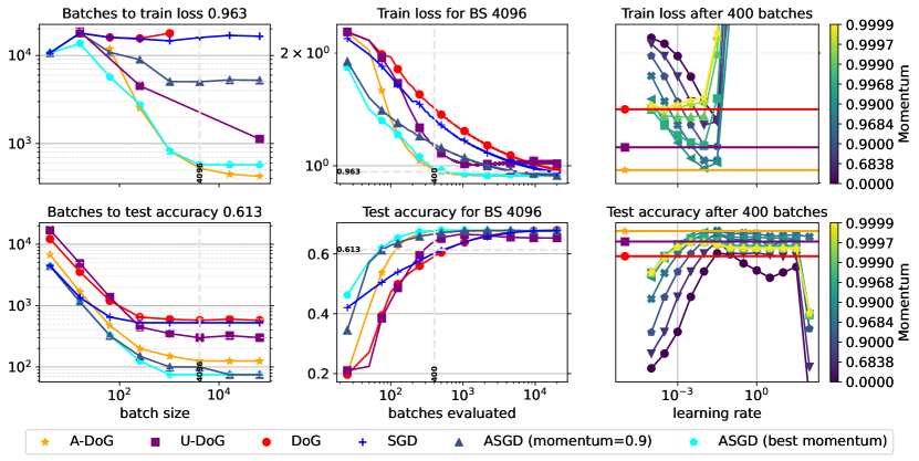
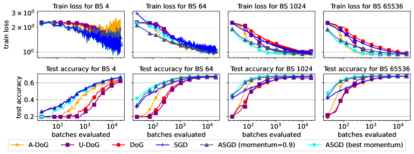
Figure 2: Training a linear model with ViT-32 features and log loss on SVHN. Top: Train loss. Bottom: Test accuracy after iterate averaging. First column: Batch size scaling of complexity to reach target performance. Second column: Learning curves. Third column: ASGD performance at all learning rates and momenta, contrasted with DoG variants.

Figure 3: Training a linear model with ViT-32 features and log loss on SVHN. Top: Loss vs. batches processed training for different batch sizes. Bottom: Test accuracy of averaged model vs. batches processed for different batch sizes.

On convex optimization problems, both U-DoG and A-DoG often substantially improve over DoG, with A-DoG achieving results comparable to well-tuned ASGD and outperforming U-DoG, likely by avoiding extra-gradient computations. Figure 1 illustrates these results on a particular dataset and least-squares loss function configuration and Section G.3 repeats this figure for additional configurations. The left panels in the figure show that the rate of convergence of A-DoG, U-DoG and ASGD plateaus at a larger batch size compared to DoG and SGD without momentum. This is the typical effect of acceleration in stochastic optimization [53], and is also supported by Corollary 2 which shows that, for sufficiently large batch size, U-DoG converges at rate scaling as $1/T^{2}$. In contrast, non-accelerated methods like DoG and SGD converge with rate scaling as $1/T$. The right panels of the figure show that, at a tight computational budget, the performance of ASGD is very sensitive to the tuning of both step size and momentum, with only the very best values matching the performance of A-DoG. When using logarithmic instead of least-squares loss, the test accuracy becomes more robust to large step size choices (see Figure 3 in the appendix). This is partly because the log loss is Lispchitz which prevents complete divergence at any fixed step size.

In our preliminary non-convex experiments on neural network models (reported in detail in Sections G.3 and G.4), we find that U-DoG often fails to converge to competitive results, while A-DoG is competitive with DoG on most VTAB tasks, but under-performs it for CIFAR-10 and ImageNet fine-tuning, indicating that it is not a yet a viable general-purpose neural network optimizer.

Appendix A Proof for Section 3 (the noiseless setting)

A.1 Proof of Proposition 1

Proof.

Define

$$\rho_{t} \coloneqq\frac{1}{\sqrt{Q_{t}}}~{}\text{and}$$

$$\hat{Q}_{t} \coloneqq\sum_{k=0}^{t}\alpha_{k}^{2}\min\left\{\|\nabla f\left(\hat{x}_{k}\right)-\nabla f\left(\hat{z}_{k}\right)\|^{2},\|g_{k}-m_{k}\|^{2}\right\}.$$

Note that in the noiseless setting $\hat{Q}_{T}=Q_{T}$. However, most of the proof carries over to the noisy setting as well. Therefore, until a later stage of the proof, we do not use that $m_{t}=\nabla f\left(\hat{z}_{t}\right)$, $g_{t}=\nabla f\left(\hat{x}_{t}\right)$ and $\hat{Q}_{t}=Q_{t}$ in the noiseless setting.

Recall the notation $\tilde{\eta}_{x,t}=\frac{1}{\sqrt{G_{x,t}}}$ and $\tilde{\eta}_{y,t}=\frac{1}{\sqrt{G_{y,t}}}$. Algebraic manipulation gives us that for all $k\geq 0$

$$\bar{r}_{k}\alpha_{k}\left<g_{k},x_{k+1}-x_{\star}\right> \leq\frac{\bar{r}_{k}^{2}\alpha_{k}^{2}\rho_{k}}{2}\|g_{k}-m_{k}\|^{2}-\sum_{k=0}^{t}\frac{1}{2\rho_{k}}\|x_{k+1}-y_{k}\|^{2}$$

$$\qquad+\left(\frac{1}{2\rho_{k}}-\frac{1}{2\tilde{\eta}_{x,k}}\right)\left(\|x_{k+1}-y_{k}\|^{2}+\|x_{k+1}-y_{k+1}\|^{2}\right)$$

$$\qquad+\frac{1}{2\tilde{\eta}_{y,k}}\left(\|x_{\star}-y_{k}\|^{2}-\|x_{\star}-y_{k+1}\|^{2}\right);$$

see Lemma 3 for a proof. Therefore, by summing over both sides of the inequality we get that for all $t\geq 0$

$$\sum_{k=0}^{t}\bar{r}_{k}\alpha_{k}\left<g_{k},x_{k+1}-x_{\star}\right> \leq\underbrace{\frac{\bar{r}_{t}^{2}}{2}\sum_{k=0}^{t}\frac{\alpha_{k}^{2}\|g_{k}-m_{k}\|^{2}}{\sqrt{\sum_{j=0}^{k}\alpha_{j}^{2}\|g_{j}-m_{j}\|^{2}}}}_{(A)}\underbrace{-\sum_{k=0}^{t}\frac{1}{2\rho_{k}}\|x_{k+1}-y_{k}\|^{2}}_{(B)}$$

$$\qquad+\underbrace{4\bar{r}_{t+1}^{2}\sum_{k=0}^{t}\left[\frac{1}{\rho_{k}}-\frac{1}{\tilde{\eta}_{x,k}}\right]_{+}}_{(C)}+\underbrace{\frac{1}{2}\sum_{k=0}^{t}\frac{1}{\tilde{\eta}_{y,k}}\left(d_{k}^{2}-d_{k+1}^{2}\right)}_{(D)}.$$

Bounding $(A)$:

We have $\sum_{k=0}^{t}\frac{\alpha_{k}^{2}\|g_{k}-m_{k}\|^{2}}{\sqrt{\sum_{j=0}^{k}\alpha_{j}^{2}\|g_{j}-m_{j}\|^{2}}}\leq 2\sqrt{\sum_{k=0}^{t}\alpha_{k}^{2}\|g_{k}-m_{k}\|^{2}}$; see Lemma 15 with $s_{k}=\alpha_{k}^{2}\|g_{k}-m_{k}\|^{2}$, and therefore

$$\frac{\bar{r}_{t}^{2}}{2}\sum_{k=0}^{t}\frac{\alpha_{k}^{2}\|g_{k}-m_{k}\|^{2}}{\sqrt{\sum_{j=0}^{k}\alpha_{j}^{2}\|g_{j}-m_{j}\|^{2}}}=\frac{\bar{r}_{t}^{2}}{\rho_{t}}.$$

Bounding $(B)$:

We have that for all $k\geq 0$

$$\|\nabla f\left(\hat{x}_{k}\right)-\nabla f\left(\hat{z}_{k}\right)\|^{2} \overset{(1)}{\leq}\beta^{2}\|\hat{x}_{k}-\hat{z}_{k}\|^{2}$$

$$=\frac{\beta^{2}\bar{r}_{k}^{2}\alpha_{k}^{2}}{\left(\sum_{0=1}^{k}\bar{r}_{i}\alpha_{i}\right)^{2}}\|x_{k+1}-y_{k}\|^{2}$$

$$\overset{(2)}{\leq}\frac{4\beta^{2}}{\alpha_{k}^{2}}\|x_{k+1}-y_{k}\|^{2},$$

where $(1)$ is from the $\beta$-smoothness of $f$, and $(2)$ is because $\bar{r}_{k}\alpha_{k}^{2}\leq 2\sum_{0=1}^{k}\bar{r}_{i}\alpha_{i}$ by Lemma 12 . Therefore,

$$-\|x_{k+1}-y_{k}\|^{2} \leq-\frac{\alpha_{k}^{2}\|\nabla f\left(\hat{x}_{k}\right)-\nabla f\left(\hat{z}_{k}\right)\|^{2}}{4\beta^{2}}.$$

Thus,

$$-\sum_{k=0}^{t}\frac{1}{2\rho_{k}}\|x_{k+1}-y_{k}\|^{2}\leq-\sum_{k=0}^{t}\frac{\alpha_{k}^{2}\|\nabla f\left(\hat{x}_{k}\right)-\nabla f\left(\hat{z}_{k}\right)\|^{2}}{8\beta^{2}\rho_{k}}$$

Bounding $(C)$:

Define

$$I\triangleq\left\{k\in\left\{0,1,\dots,t\right\}~{}:~{}\frac{1}{\rho_{t}}-\frac{1}{\tilde{\eta}_{x,t}}\geq 0\right\}.$$

Define $i_{k}$ as the $k$-th smallest index in $I$, and define $i_{\lvert I\rvert+1}\coloneqq t+1$. Thus,

$$(C) =4\bar{r}_{t+1}^{2}\sum_{k=0}^{\lvert I\rvert}\left(\frac{1}{\rho_{i_{k}}}-\frac{1}{\tilde{\eta}_{x,i_{k}}}\right)\leq 4\bar{r}_{t+1}^{2}\sum_{k=0}^{\lvert I\rvert}\left(\frac{1}{\rho_{[i_{k+1}-1]}}-\frac{1}{\tilde{\eta}_{x,i_{k}}}\right)$$

$$\leq\frac{4\bar{r}_{t+1}^{2}}{\rho_{t}}+4\bar{r}_{t+1}^{2}\sum_{k=1}^{\lvert I\rvert}\left(\frac{1}{\rho_{[i_{k}-1]}}-\frac{1}{\tilde{\eta}_{x,i_{k}}}\right)\leq\frac{4\bar{r}_{t+1}^{2}}{\rho_{t}}+4\bar{r}_{t+1}^{2}\sum_{k=0}^{t-1}\left[\frac{1}{\rho_{k}}-\frac{1}{\tilde{\eta}_{x,k+1}}\right]_{+}.$$

Bounding $(D)$:

$$\frac{1}{2}\sum_{k=0}^{t}\frac{1}{\tilde{\eta}_{y,t}}\left(d_{k}^{2}-d_{k+1}^{2}\right) =\frac{d_{0}^{2}}{2\tilde{\eta}_{y,0}}-\frac{d_{t+1}^{2}}{2\tilde{\eta}_{y,t}}+\frac{1}{2}\sum_{k=0}^{t}\left(\frac{1}{\tilde{\eta}_{y,k}}-\frac{1}{\tilde{\eta}_{y,k-1}}\right)d_{k}^{2}$$

$$\leq\frac{d_{0}^{2}}{2\tilde{\eta}_{y,0}}-\frac{d_{t+1}^{2}}{2\tilde{\eta}_{y,t}}+\frac{\bar{d}_{t}^{2}}{2}\sum_{k=0}^{t}\left(\frac{1}{\tilde{\eta}_{y,k}}-\frac{1}{\tilde{\eta}_{y,k-1}}\right).$$

By preforming telescopic summation we obtain

$$(D) \leq\frac{\bar{d}_{t+1}^{2}-d_{t+1}^{2}}{2\tilde{\eta}_{y,t}}.$$

Let $s\in\operatorname*{arg\,max}_{k\leq t+1}d_{k}$, we have that $\bar{d}_{t+1}^{2}-d_{t+1}^{2}=\bar{d}_{s}^{2}-d_{t+1}^{2}=\left(\bar{d}_{s}-d_{t+1}\right)\left(\bar{d}_{s}+d_{t+1}\right)\leq\|y_{s}-y_{t+1}\|\left(\bar{d}_{s}+d_{t+1}\right)\leq\left(\bar{r}_{s}+r_{t+1}\right)\left(\bar{d}_{s}+d_{t+1}\right)\leq 4\bar{r}_{t+1}\bar{d}_{t+1}$. Thus,

$$(D) \leq\frac{2\bar{r}_{t+1}\bar{d}_{t+1}}{\tilde{\eta}_{y,t}}.$$

Bounding $(A)+(B)+(C)+(D)$:

Combining all of the above, we obtain that

$$\sum_{k=0}^{t}\bar{r}_{k}\alpha_{k}\left<g_{k},x_{k+1}-x_{\star}\right> \leq 5\bar{r}_{t+1}\left(\bar{r}_{t+1}+\bar{d}_{t+1}\right)\max\left\{\frac{1}{\rho_{t}},\frac{1}{\tilde{\eta}_{y,t}}\right\}$$

$$\qquad+4\bar{r}_{t+1}^{2}\sum_{k=0}^{t-1}\left[\frac{1}{\rho_{k}}-\frac{1}{\tilde{\eta}_{x,k+1}}\right]_{+}-\sum_{k=0}^{t}\frac{\alpha_{k}^{2}\|\nabla f\left(\hat{x}_{k}\right)-\nabla f\left(\hat{z}_{k}\right)\|^{2}}{8\beta^{2}\rho_{k}}.$$

Therefore, as for any we have that $G_{x,k}\geq Q_{k-1}$,

$$\sum_{k=0}^{t}\bar{r}_{k}\alpha_{k}\left<g_{k},x_{k+1}-x_{\star}\right> \leq 5\bar{r}_{t+1}\left(\bar{r}_{t+1}+\bar{d}_{t+1}\right)\sqrt{\max\left\{G_{y,t},Q_{t}\right\}}-\sum_{k=0}^{t}\frac{\alpha_{k}^{2}\|\nabla f\left(\hat{x}_{k}\right)-\nabla f\left(\hat{z}_{k}\right)\|^{2}}{8\beta^{2}\rho_{k}}.$$

Let $s\geq 0$ and recall that $\frac{1}{\rho_{k}}=\sqrt{Q_{k}}$. We get that

$$\sum_{k=0}^{t}\bar{r}_{k}\alpha_{k}\left<g_{k},x_{k+1}-x_{\star}\right> \leq 10s\bar{r}_{t+1}\left(\bar{r}_{t+1}+\bar{d}_{t+1}\right)\sqrt{\hat{Q}_{t}}-\sum_{k=0}^{t}\frac{\alpha_{k}^{2}\|\nabla f\left(\hat{x}_{k}\right)-\nabla f\left(\hat{z}_{k}\right)\|^{2}}{8\beta^{2}}\sqrt{Q_{k}}$$

$$\qquad+5\bar{r}_{t+1}\left(\bar{r}_{t+1}+\bar{d}_{t+1}\right)\left(s\sqrt{Q_{t}}-2s\sqrt{\hat{Q}_{t}}\right)$$

$$\qquad+5\bar{r}_{t+1}\left(\bar{r}_{t+1}+\bar{d}_{t+1}\right)\left(\sqrt{\max\left\{G_{y,t},Q_{t}\right\}}-s\sqrt{Q_{t}}\right).$$ (16)

We have that

$$10s\bar{r}_{t+1} \left(\bar{r}_{t+1}+\bar{d}_{t+1}\right)\sqrt{\hat{Q}_{t}}-\sum_{k=0}^{t}\frac{\alpha_{t}^{2}\|\nabla f\left(\hat{x}_{t}\right)-\nabla f\left(\hat{z}_{t}\right)\|^{2}}{8\beta^{2}}\sqrt{Q_{k}}$$

$$\leq 10s\bar{r}_{t+1}\left(\bar{r}_{t+1}+\bar{d}_{t+1}\right)\sqrt{\hat{Q}_{t}}-\sum_{k=0}^{t}\frac{\alpha_{k}^{2}\min\left\{\|\nabla f\left(\hat{x}_{k}\right)-\nabla f\left(\hat{z}_{k}\right)\|^{2},\|g_{k}-m_{k}\|^{2}\right\}}{8\beta^{2}}\sqrt{\hat{Q}_{k}}.$$

Define $B_{k}^{2}=\alpha_{k}^{2}\min\left\{\|\nabla f\left(\hat{x}_{k}\right)-\nabla f\left(\hat{z}_{k}\right)\|^{2},\|g_{k}-m_{k}\|^{2}\right\}$, $c_{1}=10s\bar{r}_{t+1}(\bar{r}_{t+1}+\bar{d}_{t+1})$, and $c_{2}=8\beta^{2}$. Lemma 14 gives us that for all $t\geq 0$

$$c_{1}\sqrt{\sum_{k=0}^{t}B_{k}^{2}}-\sum_{k=0}^{t}\frac{B_{k}^{2}}{c_{2}}\sqrt{\sum_{j=0}^{k}B_{j}^{2}} \leq 2c_{1}^{3/2}c_{2}^{1/2}.$$

Therefore,

$$10s\bar{r}_{t+1} \left(\bar{r}_{t+1}+\bar{d}_{t+1}\right)\sqrt{\hat{Q}_{t}}-\sum_{k=0}^{t}\frac{\alpha_{t}^{2}\|\nabla f\left(\hat{x}_{t}\right)-\nabla f\left(\hat{z}_{t}\right)\|^{2}}{8\beta^{2}}\sqrt{Q_{k}}$$

$$\leq 2\left(10s\bar{r}_{t+1}\left(\bar{r}_{t+1}+\bar{d}_{t+1}\right)\right)^{3/2}(8\beta)^{1/2}\leq 180s^{3/2}\bar{r}_{t+1}\left(\bar{r}_{t+1}+\bar{d}_{t+1}\right)^{2}\beta.$$

Combining this result with eq. 16 yields that for all $t\geq 0$ and $s\geq 0$

$$\sum_{k=0}^{t}\bar{r}_{k}\alpha_{k}\left<g_{k},x_{k+1}-x_{\star}\right> \leq 180s^{3/2}\bar{r}_{t+1}\left(\bar{r}_{t+1}+\bar{d}_{t+1}\right)^{2}\beta$$

$$\qquad+5\bar{r}_{t+1}\left(\bar{r}_{t+1}+\bar{d}_{t+1}\right)\left(s\sqrt{Q_{t}}-2s\sqrt{\hat{Q}_{t}}\right)$$

$$\qquad+5\bar{r}_{t+1}\left(\bar{r}_{t+1}+\bar{d}_{t+1}\right)\left(\sqrt{\max\left\{G_{y,t},Q_{t}\right\}}-s\sqrt{Q_{t}}\right).$$ (17)

Lemma 1 gives us that

$$f\left(\hat{x}_{t}\right)-f(x_{\star}) \leq\frac{1}{\sum_{k=0}^{t}\bar{r}_{k}\alpha_{k}}\sum_{k=0}^{t}\bar{r}_{k}\alpha_{k}\left<\nabla f\left(\hat{x}_{k}\right),x_{k+1}-x_{\star}\right>.$$

Now, by additionally using the fact that in the noiseless setting

$$\hat{Q}_{t} =Q_{t}~{}~{}\text{and}$$

$$\sum_{k=0}^{t}\bar{r}_{k}\alpha_{k}\left<\nabla f\left(\hat{x}_{k}\right),x_{k+1}-x_{\star}\right> =\sum_{k=0}^{t}\bar{r}_{k}\alpha_{k}\left<g_{k},x_{k+1}-x_{\star}\right>$$

we get that

$$f\left(\hat{x}_{t}\right)-f(x_{\star}) \leq 180s^{3/2}\frac{\bar{r}_{t+1}}{\sum_{k=0}^{t}\bar{r}_{k}\alpha_{k}}\beta\left(\bar{r}_{t+1}+\bar{d}_{t+1}\right)^{2}$$

$$+5\frac{\bar{r}_{t+1}}{\sum_{k=0}^{t}\bar{r}_{k}\alpha_{k}}\left(\bar{r}_{t+1}+\bar{d}_{t+1}\right)\left(\sqrt{\max\left\{G_{y,t},Q_{t}\right\}}-s\sqrt{Q_{t}}\right).$$

Finally, by using the fact that $\bar{d}_{t+1}\leq d_{0}+\bar{r}_{t+1}$ and because $\bar{r}_{k}\alpha_{k}^{2}\leq 2\sum_{0=1}^{k}\bar{r}_{i}\alpha_{i}$ for all $k\geq 0$ (Lemma 12), we obtain that

$$f(\hat{x}_{t})-f(x_{\star})\leq O\left(\frac{s^{3/2}\beta\left(\bar{r}_{t+1}+d_{0}\right)^{2}+\left(\bar{r}_{t+1}+d_{0}\right)\left[\sqrt{\max\left\{G_{y,t},Q_{t}\right\}}-s\sqrt{Q_{t}}\right]_{+}}{\left(\sum_{k=0}^{t}\bar{r}_{k}/\bar{r}_{t+1}\right)^{2}}\right).$$

∎

A.2 Proof of Proposition 2

Proof.

For any $h>0$ (in this case $h=12$), define

$$c_{t} \coloneqq h\log_{+}^{2}\left(\frac{s+Q_{t-1}}{s}\right)~{}~{}\text{and}$$

$$\rho_{t} \coloneqq\frac{1}{c_{t}\sqrt{s+Q_{t}}}.$$

Lemma 3 gives us that, for all $t\geq 0$,

$$\bar{r}_{t}\alpha_{t}\left<g_{t},x_{t+1}-x_{\star}\right> \leq\frac{\bar{r}_{t}^{2}\alpha_{t}^{2}\rho_{t}}{2}\|g_{t}-m_{t}\|^{2}+\left(\frac{1}{2\rho_{t}}-\frac{1}{2\tilde{\eta}_{x,t}}\right)\left(\|x_{t+1}-y_{t}\|^{2}+\|x_{t+1}-y_{t+1}\|^{2}\right)$$

$$\qquad+\frac{1}{2\tilde{\eta}_{y,t}}\left(\|x_{\star}-y_{t}\|^{2}-\|x_{\star}-y_{t+1}\|^{2}\right).$$

From the definitions of $\rho_{t}$ and $\tilde{\eta}_{x,t}=1/\sqrt{G_{x,t}}\leq 1/\rho_{t-1}$ we obtain that

$$\frac{1}{2\rho_{t}}-\frac{1}{2\tilde{\eta}_{x,t}}\leq\frac{c_{t}^{2}}{2}\rho_{t}\left(Q_{t}-Q_{t-1}\right);$$

See proof in Lemma 13. Now, because we also have that $\max\{\|x_{t+1}-y_{t}\|,\|y_{t+1}-x_{t+1}\|\}\leq\frac{2\bar{r}_{t}}{c_{t}}$, we get

$$\bar{r}_{t}\alpha_{t}\left<g_{t},x_{t+1}-x_{\star}\right> \leq\frac{9}{2}\bar{r}_{t}^{2}\rho_{t}\alpha_{t}^{2}\|g_{t}-m_{t}\|^{2}+\frac{1}{2\tilde{\eta}_{y,t}}\left(d_{t}^{2}-d_{t+1}^{2}\right).$$

Thus,

$$2\tilde{\eta}_{y,t}\bar{r}_{t}\alpha_{t}\left<g_{t},x_{t+1}-x_{\star}\right> \leq 9\bar{r}_{t}^{2}\tilde{\eta}_{y,t}\rho_{t}\alpha_{t}^{2}\|g_{t}-m_{t}\|^{2}+\left(d_{t}^{2}-d_{t+1}^{2}\right).$$

Consequentially, by summing the two sides of the inequality, we get that for all $t\geq 0$

$$2\sum_{k=0}^{t}\tilde{\eta}_{y,k}\bar{r}_{k}\alpha_{k}\left<g_{k},x_{k+1}-x_{\star}\right> \leq 9\sum_{k=0}^{t}\bar{r}_{k}^{2}\tilde{\eta}_{y,k}\rho_{k}\alpha_{k}^{2}\|g_{k}-m_{k}\|^{2}+\sum_{k=0}^{t}\left(d_{k}^{2}-d_{k+1}^{2}\right)$$

$$\leq\frac{9\bar{r}_{t}^{2}}{h^{2}}\sum_{k=0}^{t}\frac{Q_{k}-Q_{k-1}}{\left(s+Q_{k}\right)\log_{+}^{2}\left(\frac{s+Q_{k}}{s}\right)}+\sum_{k=0}^{t}\left(d_{k}^{2}-d_{k+1}^{2}\right).$$

Lemma 17 gives us that

$$\sum_{k=0}^{t}\frac{Q_{k}-Q_{k-1}}{\left(s+Q_{k}\right)\log_{+}^{2}\left(\frac{s+Q_{k}}{s}\right)}\leq 1.$$

Therefore, we obtain that

$$2\sum_{k=0}^{t}\tilde{\eta}_{y,k}\bar{r}_{k}\alpha_{k}\left<g_{k},x_{k+1}-x_{\star}\right> \leq\frac{9\bar{r}_{t}^{2}}{h^{2}}+\sum_{k=0}^{t}\left(d_{k}^{2}-d_{k+1}^{2}\right).$$

Thus,

$$2\sum_{k=0}^{t}\tilde{\eta}_{y,k}\bar{r}_{k}\alpha_{k}\left<\nabla f\left(\hat{x}_{k}\right),x_{k+1}-x_{\star}\right>\leq \frac{9\bar{r}_{t}^{2}}{h^{2}}+2\sum_{k=0}^{t}\tilde{\eta}_{y,k}\bar{r}_{k}\alpha_{k}\left<\nabla f\left(\hat{x}_{k}\right)-g_{k},x_{k+1}-x_{\star}\right>$$

$$+\sum_{k=0}^{t}\left(d_{k}^{2}-d_{k+1}^{2}\right).$$

Consequentially, as Lemma 4 gives us that

$$\sum_{k=0}^{t}\tilde{\eta}_{y,k}\bar{r}_{k}\alpha_{k}\left<\nabla f\left(\hat{x}_{k}\right),x_{k+1}-x_{\star}\right>\geq 0,$$

we get that

$$0\leq\frac{9\bar{r}_{t}^{2}}{h^{2}}+2\sum_{k=0}^{t}\eta_{y,k}\alpha_{k}\left<\nabla f\left(\hat{x}_{k}\right)-g_{k},x_{k+1}-x_{\star}\right>+\sum_{k=0}^{t}\left(d_{k}^{2}-d_{k+1}^{2}\right).$$

Therefore, we get that for all $t\geq 0$

$$d_{t+1}^{2}\leq\frac{9\bar{r}_{t}^{2}}{h^{2}} +2\sum_{k=0}^{t}\eta_{y,k}\alpha_{k}\left<\nabla f\left(\hat{x}_{k}\right)-g_{k},x_{k+1}-x_{\star}\right>+d_{0}^{2}.$$ (18)

As we are in the noiseless case, and $h=12$, we get that for all $t\geq 0$

$$d_{t+1}^{2} \leq\frac{\bar{r}_{t}^{2}}{16}+d_{0}^{2}$$

$$\leq\left(d_{0}+\frac{1}{4}\bar{r}_{t}\right)^{2}.$$

Finally, Lemma 5 now gives us that for all $t\geq 0$

$$d_{t}\leq 2d_{0}~{}~{}\text{and}~{}~{}r_{t}\leq 4d_{0}.$$

∎

A.3 Proof of Theorem 1

Proof.

Define

$$c_{t}=12\log_{+}^{2}\left(\frac{\|m_{0}\|^{2}+Q_{t}}{\|m_{0}\|^{2}}\right).$$

From Lemma 6, we get that for all $t\geq 0$ the distance between iterates is not large:

$$\max\left\{\|x_{t+1}-y_{t}\|,\|x_{t+1}-y_{t+1}\|\right\} \leq\frac{2\bar{r}_{t}}{c_{t-1}}.$$

Now, we fulfill all the conditions for Proposition 2 and therefore, for all $t\geq 0$

$$\bar{d}_{t}\leq 2d_{0}~{}~{}\text{and}~{}~{}\bar{r}_{t}\leq 4d_{0}.$$

Proposition 1 gives that for all $t\geq 0$ and for all $s\geq 0$

$$f(\hat{x}_{t})-f(x_{\star})\leq O\left(\frac{s^{3/2}\beta\left(\bar{r}_{t+1}+d_{0}\right)^{2}+\left(\bar{r}_{t+1}+d_{0}\right)\left[\sqrt{G_{y,t}}-s\sqrt{Q_{t}}\right]_{+}}{\left(\sum_{k=0}^{t}\bar{r}_{k}/\bar{r}_{t+1}\right)^{2}}\right).$$

By using the fact that $\bar{r}_{t}\leq 4d_{0}$, we get that for all $t\geq 0$

$$f(\hat{x}_{t})-f(x_{\star})\leq O\left(\frac{s^{3/2}\beta d_{0}^{2}+d_{0}\left[\sqrt{G_{y,t}}-s\sqrt{Q_{t}}\right]_{+}}{\left(\sum_{k=0}^{t}\bar{r}_{k}/\bar{r}_{t+1}\right)^{2}}\right).$$ (19)

Recall that

$$\tau=\operatorname*{arg\,max}_{t<T}\sum_{i\leq t}\frac{\bar{r}_{i}}{\bar{r}_{t+1}}.$$

To show the non-smooth rate, we set $s=0$ and obtain

$$\sqrt{G_{y,\tau}} \leq c_{T}\sqrt{\max_{k\leq T-1}\left\{\alpha_{k}^{2}\|m_{k}\|^{2}\right\}+\sum_{k=0}^{T-1}\alpha_{k}^{2}\|g_{k}-m_{k}\|^{2}}\leq c_{T}\sqrt{T^{2}L^{2}+T^{3}L^{2}}\leq 2LT^{3/2}c_{T}.$$

This result, with eq. 19, gives us that

$$f(\hat{x}_{\tau})-f(x_{\star})\leq O\left(\frac{Ld_{0}T^{3/2}}{\left(\sum_{k=0}^{\tau}\bar{r}_{k}/\bar{r}_{t+1}\right)^{2}}c_{T}\right).$$ (20)

To show the smooth rate, setting $s=2c_{t+1}$ yields

$$\sqrt{G_{y,t}}-s\sqrt{Q_{t}} \leq c_{t+1}\left(\sqrt{Q_{t}+M_{t}}-2\sqrt{Q_{t}}\right)\leq c_{t+1}\left(\sqrt{M_{t}}-\sqrt{Q_{t}}\right).$$

For some $\kappa_{t}\leq t$ we have that $\sqrt{M_{t}}=\alpha_{\kappa_{t}}\|m_{\kappa_{t}}\|$. In addition, the smoothness of $f$ implies that $\|\nabla f(z)\|^{2}\leq 2\beta[f(z)-f(x_{\star})]$ for all $z\in\mathcal{X}$. Combining this fact with the triangle inequality gives us that, in the noiseless setting,

$$\alpha_{\kappa_{t}}\|m_{\kappa_{t}}\|=\alpha_{\kappa_{t}}\|\nabla f\left(\hat{z}_{\kappa_{t}}\right)\| \leq\alpha_{\kappa_{t}}\|\nabla f\left(\hat{x}_{\kappa_{t}}\right)-\nabla f\left(\hat{z}_{\kappa_{t}}\right)\|+\alpha_{\kappa_{t}}\sqrt{2\beta}\sqrt{f(\hat{x}_{\kappa_{t}})-f(x_{\star})}.$$

Thus,

$$\sqrt{M_{t}} \leq\sqrt{Q_{t}}+\alpha_{\kappa_{t}}\sqrt{2\beta}\sqrt{f(\hat{x}_{\kappa_{t}})-f(x_{\star})}.$$

Therefore,

$$\sqrt{G_{y,t}}-s\sqrt{Q_{t}} \leq\alpha_{\kappa_{t}}\sqrt{2c_{t+1}^{2}\beta}\sqrt{f(\hat{x}_{\kappa_{t}})-f(x_{\star})}.$$

This result, together with eq. 19, give us that for all $t\geq 0$, there exist $\kappa_{t}\leq t$ such as

$$f(\hat{x}_{t})-f(x_{\star})\leq O\left(\frac{c_{t+1}^{3/2}\beta d_{0}^{2}+\alpha_{\kappa_{t}}\sqrt{c_{t+1}^{2}\beta d_{0}^{2}}\sqrt{f(\hat{x}_{\kappa_{t}})-f(x_{\star})}}{\left(\sum_{k=0}^{t}\bar{r}_{k}/\bar{r}_{t+1}\right)^{2}}\right).$$

Using the previous inequality and Lemma 2 we obtain that for all $t\geq 0$ that

$$f(\hat{x}_{t})-f(x_{\star})\leq O\left(\frac{\beta d_{0}^{2}}{\left(\sum_{k=0}^{t}\bar{r}_{k}/\bar{r}_{t+1}\right)^{2}}c_{t+1}^{2}\right).$$ (21)

Combining the result from eq. 20 and eq. 21 gives

$$f(\hat{x}_{\tau})-f(x_{\star})\leq O\left(\frac{\min\left\{\beta d_{0}^{2},Ld_{0}T^{3/2}\right\}}{\left(\sum_{k=0}^{\tau}\bar{r}_{k}/\bar{r}_{t+1}\right)^{2}}c_{T}^{2}\right).$$ (22)

Lemma 16 gives us that

$$\sum_{k=0}^{\tau}\bar{r}_{k}/\bar{r}_{t+1}\geq\frac{1}{e}\left(\frac{T}{\log_{+}(\bar{r}_{T}/r_{\epsilon})}-1\right).$$

Thus, if $T\geq 2\log_{+}(\bar{r}_{T}/r_{\epsilon})$ then

$$\frac{1}{\sum_{k=0}^{\tau}\bar{r}_{k}/\bar{r}_{t+1}}\leq O\left(\frac{1}{T}\log_{+}\left(\frac{\bar{r}_{T}}{r_{\epsilon}}\right)\right).$$

Therefore, from eq. 22, we obtain

$$f(\hat{x}_{\tau})-f(x_{\star})\leq O\left(\frac{\min\left\{\beta d_{0}^{2},Ld_{0}T^{3/2}\right\}}{T^{2}}c_{T}^{2}\log_{+}^{2}\left(\frac{\bar{r}_{T}}{r_{\epsilon}}\right)\right).$$ (23)

We have that

$$c_{T} \leq O\left(\log_{+}^{2}\left(\frac{\|m_{0}\|^{2}+Q_{T-1}}{\|m_{0}\|^{2}}\right)\right)$$

$$\overset{(i)}{\leq}O\left(\log_{+}^{2}\left(1+\frac{T^{3}\min\left\{\beta d_{0},L\right\}}{\|\nabla f\left(\hat{z}_{0}\right)\|^{2}}\right)\right)\leq O\left(\log_{+}^{2}\left(1+T\frac{\min\left\{\beta d_{0}^{2},Ld_{0}\right\}}{f(x_{0})-f(x_{\star})}\right)\right),$$

due to $(i)$ the noiseless setting and $f$ being $\beta$-smooth and $L$-Lipschitz, and $(ii)$ convexity, which implies $f(x_{0})-f(x_{\star})\leq d_{0}\|\nabla f\left(\hat{z}_{0}\right)\|$ Finally, from eq. 23, we obtain

$$f(\hat{x}_{\tau})-f(x_{\star})\leq O\left(\frac{\min\left\{\beta d_{0}^{2},Ld_{0}T^{3/2}\right\}}{T^{2}}\log_{+}^{4}\left(1+T\frac{\min\left\{\beta d_{0}^{2},Ld_{0}\right\}}{f(x_{0})-f(x_{\star})}\right)\log_{+}^{2}\left(\frac{d_{0}}{r_{\epsilon}}\right)\right).$$ (24)

Finally, for $T\leq 2\log_{+}(\bar{r}_{T}/r_{\epsilon})$ the theorem holds trivially since $f(\hat{x}_{\tau})-f(x_{\star})\leq\min\left\{\beta\bar{d}_{\tau}^{2},L\bar{d}_{\tau}\right\}$ and $\bar{d}_{\tau}\leq 2d_{0}$ by Proposition 4. Therefore,

$$f(\hat{x}_{\tau})-f(x_{\star})\leq O\left(\min\left\{\beta d_{0}^{2},Ld_{0}\right\}\right)\leq O\left(\frac{\min\left\{\beta\bar{d}_{0}^{2},L\bar{d}_{0}\right\}}{T^{2}}\log_{+}^{2}(\bar{r}_{T}/r_{\epsilon})\right),$$

and so the bound Equation 24 holds in all cases, concluding the proof. ∎

Appendix B Proofs for Section 4 (the stochastic setting)

B.1 Proof of Proposition 3

Proof.

Define

$$\hat{Q}_{t}\coloneqq\sum_{k=0}^{t}\alpha_{k}^{2}\min\left\{\|\nabla f\left(\hat{x}_{k}\right)-\nabla f\left(\hat{z}_{k}\right)\|^{2},\|g_{k}-m_{k}\|^{2}\right\}.$$

Our proof continues from eq. 17 in the proof Proposition 1, which also holds for stochastic gradients.

$$\sum_{k=0}^{t}\bar{r}_{k}\alpha_{k}\left<g_{k},x_{k+1}-x_{\star}\right> \leq 180s^{3/2}\bar{r}_{t+1}\left(\bar{r}_{t+1}+\bar{d}_{t+1}\right)^{2}\beta$$

$$\qquad+5\bar{r}_{t+1}\left(\bar{r}_{t+1}+\bar{d}_{t+1}\right)\left(s\sqrt{Q_{t}}-2s\sqrt{\hat{Q}_{t}}\right)$$

$$\qquad+5\bar{r}_{t+1}\left(\bar{r}_{t+1}+\bar{d}_{t+1}\right)\left(\sqrt{\max\left\{G_{y,t},Q_{t}\right\}}-s\sqrt{Q_{t}}\right).$$

For all $k\geq 0$

$$\|g_{k}-m_{k}\|^{2} \leq 2\|\nabla f\left(\hat{x}_{k}\right)-\nabla f\left(\hat{z}_{k}\right)\|^{2}+2\|(g_{k}-\nabla f\left(\hat{x}_{k}\right))-(m_{k}-\nabla f\left(\hat{z}_{k}\right))\|^{2}$$

$$\leq 2\min\left\{\|\nabla f\left(\hat{x}_{k}\right)-\nabla f\left(\hat{z}_{k}\right)\|^{2},\|g_{k}-m_{k}\|^{2}\right\}+4\|m_{t}-\nabla f\left(\hat{z}_{t}\right)\|^{2}+4\|g_{t}-\nabla f\left(\hat{x}_{t}\right)\|^{2}.$$

Thus, for all $k\geq 0$

$$\|g_{k}-m_{k}\|^{2} \leq 2\min\left\{\|\nabla f\left(\hat{x}_{k}\right)-\nabla f\left(\hat{z}_{k}\right)\|^{2},\|g_{k}-m_{k}\|^{2}\right\}+4\|m_{t}-\nabla f\left(\hat{z}_{t}\right)\|^{2}+4\|g_{t}-\nabla f\left(\hat{x}_{t}\right)\|^{2}.$$

Multiplying by $\alpha_{k}^{2}$, summing and recalling that $\alpha_{k}\leq k+1$ implies $Q_{t}\leq 2\hat{Q}_{t}+4(t+1)^{3}V_{t}$, where $V_{t}=\frac{1}{t+1}\sum_{k=0}^{t}\left(\|g_{t}-\nabla f\left(\hat{x}_{t}\right)\|^{2}+\|m_{t}-\nabla f\left(\hat{z}_{t}\right)\|^{2}\right)$ is the empirical variance. Substituting into eq. 17, we get that

$$\sum_{k=0}^{t}\bar{r}_{k}\alpha_{k}\left<g_{k},x_{k+1}-x_{\star}\right> \leq 180s^{3/2}\bar{r}_{t+1}\left(\bar{r}_{t+1}+\bar{d}_{t+1}\right)^{2}\beta$$

$$\qquad+5\bar{r}_{t+1}\left(\bar{r}_{t+1}+\bar{d}_{t+1}\right)\left(\sqrt{\max\left\{G_{y,t},Q_{t}\right\}}-s\sqrt{Q_{t}}\right)$$

$$\qquad+10s\bar{r}_{t+1}\left(\bar{r}_{t+1}+\bar{d}_{t+1}\right)\sqrt{(t+1)^{3}V_{t}}.$$ (25)

Lemma 8 gives us that with probability of at least $1-\delta-\mathbb{P}\left[\bar{\mathfrak{b}}_{T-1}>\mathfrak{B}\right]$, for all $t\in\left\{0,1,\dots,T-1\right\}$,

$$\left\lvert\sum_{k=0}^{t}\bar{r}_{t}\alpha_{k}\left<\nabla f\left(\hat{x}_{k}\right)-g_{k},x_{k+1}-x_{\star}\right>\right\rvert \leq 8\alpha_{t}\bar{r}_{t}\bar{d}_{t+1}\sqrt{\theta_{t+1,\delta}\sum_{k=0}^{t}\|\nabla f\left(\hat{x}_{k}\right)-g_{k}\|^{2}+\left(\theta_{t+1,\delta}\mathfrak{B}\right)^{2}}.$$

Using the previous equality and the definition of $V_{t}$ we obtain that

$$\sum_{k=0}^{t}\bar{r}_{k}\alpha_{k} \left<\nabla f\left(\hat{x}_{k}\right),x_{k+1}-x_{\star}\right>$$

$$=\sum_{k=0}^{t}\bar{r}_{k}\alpha_{k}\left<g_{k},x_{k+1}-x_{\star}\right>+\sum_{k=0}^{t}\bar{r}_{k}\alpha_{k}\left<\nabla f\left(\hat{x}_{k}\right)-g_{k},x_{k+1}-x_{\star}\right>$$

$$\leq\sum_{k=0}^{t}\bar{r}_{k}\alpha_{k}\left<g_{k},x_{k+1}-x_{\star}\right>+8\alpha_{t}\bar{r}_{t}\bar{d}_{t+1}\sqrt{(t+1)\theta_{t+1,\delta}V_{t}+\left(\theta_{t+1,\delta}\mathfrak{B}\right)^{2}}.$$ (26)

Lemma 1 gives us that

$$f\left(\hat{x}_{t}\right)-f(x_{\star}) \leq\frac{1}{\sum_{k=0}^{t}\bar{r}_{k}\alpha_{k}}\sum_{k=0}^{t}\bar{r}_{k}\alpha_{k}\left<\nabla f\left(\hat{x}_{k}\right),x_{k+1}-x_{\star}\right>.$$

By combining the above inequality with eq. 25 and eq. 26, we obtain

$$f\left(\hat{x}_{t}\right)-f(x_{\star}) \leq 180s^{3/2}\frac{\bar{r}_{t+1}}{\sum_{k=0}^{t}\bar{r}_{k}\alpha_{k}}\beta\left(\bar{r}_{t+1}+\bar{d}_{t+1}\right)^{2}$$

$$+5\frac{\bar{r}_{t+1}}{\sum_{k=0}^{t}\bar{r}_{k}\alpha_{k}}\left(\bar{r}_{t+1}+\bar{d}_{t+1}\right)\left(\sqrt{\max\left\{G_{y,t},Q_{t}\right\}}-s\sqrt{Q_{t}}\right)$$

$$+10\left(1+s\right)\frac{\bar{r}_{t+1}}{\sum_{k=0}^{t}\bar{r}_{k}\alpha_{k}}\left(\bar{r}_{t+1}+\bar{d}_{t+1}\right)\sqrt{(t+1)^{3}V_{t}+\left(\theta_{t+1,\delta}\mathfrak{B}\right)^{2}}.$$

Now, as Lemma 12 gives us that $\bar{r}_{t}\alpha_{t}^{2}\leq 2\sum_{k=0}^{t}\bar{r}_{k}\alpha_{k}$, we obtain that

$$f\left(\hat{x}_{t}\right)-f(x_{\star}) \leq 360s^{3/2}\frac{1}{\left(\sum_{k=0}^{t}\bar{r}_{k}/\bar{r}_{t+1}\right)^{2}}\beta\left(\bar{r}_{t+1}+\bar{d}_{t+1}\right)^{2}$$

$$+10\frac{1}{\left(\sum_{k=0}^{t}\bar{r}_{k}/\bar{r}_{t+1}\right)^{2}}\left(\bar{r}_{t+1}+\bar{d}_{t+1}\right)\left(\sqrt{\max\left\{G_{y,t},Q_{t}\right\}}-s\sqrt{Q_{t}}\right)$$

$$+20\frac{1}{\left(\sum_{k=0}^{t}\bar{r}_{k}/\bar{r}_{t+1}\right)^{2}}\left(\bar{r}_{t+1}+\bar{d}_{t+1}\right)\sqrt{(t+1)^{3}V_{t}+\left(\theta_{t+1,\delta}\mathfrak{B}\right)^{2}}.$$

Finally, because that $\bar{d}_{t+1}\leq d_{0}+\bar{r}_{t+1}$, we get that for any $\mathfrak{B}>0$ with probability of at least $1-\delta-\mathbb{P}[\bar{\mathfrak{b}}_{T-1}>\mathfrak{B}]$ we have that for all $t<T$ and for any number $s\geq 0$

$$f(\hat{x}_{t})-f(x_{\star}) \leq O\left(\text{RHS}_{\lx@cref{creftype~refnum}{eq:noiseless-subopt}}+\frac{(1+s)\left(\bar{r}_{t+1}+d_{0}\right)\sqrt{t^{3}\theta_{t,\delta}V_{t}+\left(t\theta_{t,\delta}\mathfrak{B}\right)^{2}}}{\left(\sum_{k=0}^{t}\bar{r}_{k}/\bar{r}_{t+1}\right)^{2}}\right)$$

where $\text{RHS}_{\lx@cref{creftype~refnum}{eq:noiseless-subopt}}=\frac{s^{3/2}\beta\left(\bar{r}_{t+1}+d_{0}\right)^{2}+\left(\bar{r}_{t+1}+d_{0}\right)\left[\sqrt{\max\left\{G_{y,t},Q_{t}\right\}}-s\sqrt{Q_{t}}\right]_{+}}{\left(\sum_{k=0}^{t}\bar{r}_{k}/\bar{r}_{t+1}\right)^{2}}$ is the error term appearing in Proposition 1. ∎

B.2 Proof of Proposition 4

Proof.

The proof continues from eq. 18 in the proof of Proposition 2, which also holds for stochastic gradients. Substituting $h=400$ in eq. 18 gives, for all $t\geq 0$,

$$d_{t+1}^{2}\leq\frac{9\bar{r}_{t}^{2}}{400^{2}} +2\sum_{k=0}^{t}\eta_{y,k}\alpha_{k}\left<\nabla f\left(\hat{x}_{k}\right)-g_{k},x_{k+1}-x_{\star}\right>+d_{0}^{2}.$$

Now, Lemma 9 gives us that with probability at least $1-\delta$, for all $t<T$

$$\left\lvert\sum_{k=0}^{t}\alpha_{k}\eta_{y,k}\left<g_{k}-\nabla f\left(\hat{x}_{k}\right),x_{k+1}-x_{\star}\right>\right\rvert \leq\frac{12\theta_{t+1,\delta}}{400\theta_{T,\delta}}\bar{r}_{t}\bar{d}_{t+1}$$

$$\leq\frac{12\theta_{t+1,\delta}}{400\theta_{T,\delta}}\left(\bar{r}_{t}\bar{r}_{t+1}+\bar{r}_{t}d_{0}\right)\leq\frac{12}{400}\left(1+\frac{3}{400}\right)\bar{r}_{t}^{2}+\frac{12}{400}\bar{r}_{t}d_{0}.$$

Therefore,

$$d_{t+1}^{2}\leq\frac{81\bar{r}_{t}^{2}}{400^{2}} +\frac{24}{400}\bar{r}_{t}^{2}+\frac{24}{400}\bar{r}_{t}d_{0}+d_{0}^{2}\leq\frac{\bar{r}_{t}^{2}}{16}+\frac{\bar{r}_{t}d_{0}}{2}+d_{0}.$$

Thus, with probability of at least $1-\delta$, for all $t<T$

$$d_{t+1}^{2} \leq\left(d_{0}+\frac{1}{4}\bar{r}_{t}\right)^{2}.$$

Finally, Lemma 5 gives us that with probability of at least $1-\delta$ for all $t<T$

$$d_{t}\leq 2d_{0}~{}~{}\text{and}~{}~{}r_{t}\leq 4d_{0}.$$

∎

B.3 Proof of Theorem 2

Proof.

Recall the notation

$$\tilde{q}_{t}\coloneqq 2\alpha_{t}^{2}\|\tilde{g}_{t}-m_{t}\|^{2}~{}~{}\mbox{,}~{}~{}\bar{Q}_{t}\coloneqq\sum_{k=0}^{t}\max\left\{q_{k},\tilde{q}_{k}\right\}~{}~{}\mbox{and}~{}~{}p_{t}\coloneqq 8\left(t+1\right)^{2}\bar{\mathfrak{b}}_{t}^{2},$$

and that our step sizes are of the form (2) with

$$G_{y,t}=\hat{c}_{t}^{2}\max\left\{\|m_{0}\|^{2}+p_{0}+p_{t}+\tilde{q}_{t}+\bar{Q}_{t-1},M_{t}\right\},$$

where

$$\hat{c}_{t}=400\theta_{T,\delta}\log_{+}^{2}\left(1+\frac{p_{t}+\tilde{q}_{t}+\bar{Q}_{t-1}}{\|m_{0}\|^{2}+p_{0}}\right).$$

We begin by verifying the conditions of Proposition 4 with $s=\|m_{0}\|^{2}+p_{0}$, where condition $(iv)$ holds by construction. By Assumption 3 we have

$$\|g_{t}-\tilde{g}_{t}\|^{2}\leq 2\|g_{t}-\nabla f\left(\hat{x}_{t}\right)\|^{2}+2\|\tilde{g}_{t}-\nabla f\left(\hat{x}_{t}\right)\|^{2}\leq 4\bar{\mathfrak{b}}_{t}^{2}.$$

Therefore, since $t+1\geq\alpha_{t}$, we have

$$\tilde{q}_{t}+p_{t}\geq\alpha_{t}^{2}\left(2\|\tilde{g}_{t}-m_{t}\|^{2}+2\|g_{t}-\tilde{g}_{t}\|^{2}\right)\geq\alpha_{t}^{2}\|g_{t}-m_{t}\|^{2}=q_{t},$$

and consequently

$$\tilde{q}_{t}+p_{t}+\bar{Q}_{t-1}\geq Q_{t}.$$

Defining

$$c_{t}=400\theta_{T,\delta}\log_{+}^{2}\left(1+\frac{Q_{t}}{\|m_{0}\|^{2}+p_{0}}\right),$$

we conclude that

$$G_{y,t}\geq c_{t}^{2}\max\left\{\|m_{0}\|^{2}+p_{0}+Q_{t},M_{t}\right\}\geq c_{t}^{2}(\|m_{0}\|^{2}+p_{0}+Q_{t})$$

so that condition $(i)$ of Proposition 4 holds. Next, since

$$G_{y,t}\geq c_{t}^{2}\max\{Q_{t},M_{t}\}\geq c_{t}^{2}\alpha_{t}^{2}\max\{\|g_{t}-m_{t}\|^{2},\|m_{t}\|^{2}\},$$

Lemma 6 guarantees condition $(ii)$ of Proposition 4. Finally, we note that

$$p_{t}\geq 8\alpha_{t}^{2}\max\{\|g_{t}-\nabla f\left(\hat{x}_{t}\right)\|^{2},\|\tilde{g}_{t}-\nabla f\left(\hat{x}_{t}\right)\|^{2}\}$$

and

$$p_{t}+\tilde{q}_{t}\geq\alpha_{t}^{2}\left(2\|m_{t}-\tilde{g}_{t}\|^{2}+2\|\tilde{g}_{t}-\nabla f\left(\hat{x}_{t}\right)\|^{2}\right)\geq\alpha_{t}^{2}\|m_{t}-\nabla f\left(\hat{x}_{t}\right)\|^{2}.$$

Therefore, as $\sqrt{G_{y,t}}\geq c_{t}\sqrt{p_{t}+\tilde{q}_{t}}$, condition $(iii)$ of Proposition 4 holds.

As all the conditions for Proposition 4 hold, with probability of at least $1-\delta$, for all $t\geq 0$

$$\bar{d}_{t}\leq 2d_{0}~{}~{}\text{and}~{}~{}\bar{r}_{t}\leq 4d_{0}.$$

Recalling that $\mathfrak{b}_{\star}\coloneqq\max_{x:\|x-x_{\star}\|\leq 2d_{0}}\left\{\mathfrak{b}(x)\right\}$, this also implies that $\mathbb{P}[\bar{\mathfrak{b}}_{T-1}>\mathfrak{b}_{\star}]\leq\delta$.

We now combine the conclusions of Proposition 4 with Proposition 1 to obtain a suboptimality bound for U-DoG. Substituting $\mathbb{P}\left(\bar{r}_{T}\leq 4d_{0}\right)\leq\delta$ and $\mathbb{P}[\bar{\mathfrak{b}}_{T-1}>\mathfrak{b}_{\star}]\leq\delta$ into Proposition 3 we get that, with probability at least $1-3\delta$, for all $t<T$ and $s\geq 0$,

$$f(\hat{x}_{t})-f(x_{\star}) \leq O\left(\frac{s^{3/2}\beta d_{0}^{2}+d_{0}\left[\sqrt{G_{y,t}}-s\sqrt{Q_{t}}\right]_{+}+(1+s)d_{0}\sqrt{t^{3}\theta_{t+1,\delta}V_{t}+\left(t\theta_{t+1,\delta}\mathfrak{b}_{\star}\right)^{2}}}{\left(\sum_{k=0}^{t}\bar{r}_{k}/\bar{r}_{t+1}\right)^{2}}\right).$$ (27)

To simplify $G_{y,t}$ in the bound above, we invoke Lemma 10 which gives that, with probability at least $1-\delta-\mathbb{P}[\bar{\mathfrak{b}}_{T-1}>\mathfrak{b}_{\star}]\geq 1-2\delta$, for all $t<T$,

$$\bar{Q}_{t}\leq 5Q_{t}+80\left(t+1\right)^{3}\sqrt{\theta_{t+1,\delta}}V_{t}+2\left(t+1\right)^{2}\theta_{t+1,\delta}\mathfrak{b}_{\star}^{2},$$

and hence

$$\sqrt{G_{y,t}}\leq\hat{c}_{t}\sqrt{\bar{Q}_{t}+2M_{t}+2p_{t}}=O\left(\hat{c}_{t}\sqrt{Q_{t}}+\hat{c}_{t}\sqrt{M_{t}}+\hat{c}_{t}\theta_{T,\delta}\sqrt{t^{3}V_{t}+t^{2}\mathfrak{b}_{\star}^{2}}\right).$$

Combining this with the bound (27) and replacing $s$ with $s\hat{c}_{t}\sqrt{3}$, we get that with probability at least $1-5\delta$, for all $t<T$ and $s\geq 0$,

$$f(\hat{x}_{t})-f(x_{\star}) \leq O\left(\frac{s^{3/2}\hat{c}_{t}^{3/2}\beta d_{0}^{2}+\hat{c}_{t}d_{0}\left(\left[(1-s)\sqrt{Q_{t}}+\sqrt{M_{t}}\right]_{+}+(1+s)\theta_{T,\delta}\sqrt{t^{3}V_{t}+t^{2}\mathfrak{b}_{\star}^{2}}\right)}{\left(\sum_{k=0}^{t}\bar{r}_{k}/\bar{r}_{t+1}\right)^{2}}\right).$$ (28)

The remainder of the proof parallels the proof of Theorem 1, where we specialize our bound to the Lipschitz and smooth cases by choosing different values of $s$. For the Lipschitz case, we use the facts that

$$Q_{t}\leq 4\sum_{k\leq T}\alpha_{t}^{2}\left(\|\nabla f\left(\hat{x}_{k}\right)\|^{2}+\|\nabla f\left(\hat{z}_{k}\right)\|^{2}+\|g_{k}-\nabla f\left(\hat{x}_{k}\right)\|^{2}+\|m_{k}-\nabla f\left(\hat{z}_{k}\right)\|^{2}\right)=O(L^{2}T^{3}+V_{T}T^{3})$$

$Q_{t}=O(L^{2}T^{3})$ and $M_{t}\leq O(L^{2}T^{2})$ and (under the event $\bar{d}_{T}\leq 2d_{0}$)

$$M_{t}\leq\max_{k\leq T}\left\{2\alpha_{t}^{2}\left(\|\nabla f\left(\hat{z}_{k}\right)\|^{2}+\|m_{k}-\nabla f\left(\hat{z}_{k}\right)\|^{2}\right)\right\}=O(L^{2}T^{2}+\mathfrak{b}_{\star}^{2}T^{2}),$$

giving the suboptimality bound. Substituting these expression and $s=0$ into (28) we get, for all $t<T$,

$$f(\hat{x}_{t})-f(x_{\star}) \leq O\left(\hat{c}_{t}\frac{Ld_{0}T^{3/2}+d_{0}\theta_{T,\delta}\sqrt{T^{3}V_{T}+T^{2}\mathfrak{b}_{\star}^{2}}}{\left(\sum_{k=0}^{t}\bar{r}_{k}/\bar{r}_{t+1}\right)^{2}}\right).$$ (29)

For the smooth case and any $t<T$, let $\kappa_{t}\leq t$ be such that For some $\kappa_{t}\leq t$ we have that

$$\sqrt{M_{t}}=\alpha_{\kappa_{t}}\|m_{\kappa_{t}}\|.$$

The smoothness of $f$ implies that $\|\nabla f(z)\|^{2}\leq 2\beta[f(z)-f(x_{\star})]$ for all $z\in\mathcal{X}$. Combining this fact with the triangle inequality gives us that

$$\alpha_{\kappa_{t}}\|m_{\kappa_{t}}\|\leq\alpha_{\kappa_{t}}\|\nabla f\left(\hat{x}_{\kappa_{t}}\right)-\nabla f\left(\hat{z}_{\kappa_{t}}\right)\|+\alpha_{\kappa_{t}}\|m_{\kappa_{t}}-\nabla f\left(\hat{z}_{\kappa_{t}}\right)\|+\alpha_{\kappa_{t}}\sqrt{2\beta}\sqrt{f(\hat{x}_{\kappa_{t}})-f(x_{\star})}$$

and therefore,

$$\sqrt{M_{t}} \leq\sqrt{Q_{t}}+\sqrt{(t+1)^{3}V_{t}}+\alpha_{\kappa_{t}}\sqrt{2\beta}\sqrt{f(\hat{x}_{\kappa_{t}})-f(x_{\star})}.$$

Substituting into eq. 28 and taking $s=2$, we get, for all $t<T$,

$$f(\hat{x}_{t})-f(x_{\star})\leq O\left(\frac{\hat{c}_{t}^{3/2}\beta d_{0}^{2}+\hat{c}_{t}d_{0}\theta_{T,\delta}\sqrt{T^{3}V_{T}+T^{2}\mathfrak{b}_{\star}^{2}}+\alpha_{\kappa_{t}}\sqrt{\hat{c}_{t+1}^{2}\beta d_{0}^{2}}\sqrt{f(\hat{x}_{\kappa_{t}})-f(x_{\star})}}{\left(\sum_{k=0}^{t}\bar{r}_{k}/\bar{r}_{t+1}\right)^{2}}\right).$$

Applying Lemma 2 and noting that $\theta_{T,\delta}\leq\hat{c}_{t}$ simplifies the bound to

$$f(\hat{x}_{t})-f(x_{\star})\leq O\left(\frac{\hat{c}_{T}^{2}\beta d_{0}^{2}+\hat{c}_{T}\theta_{T,\delta}d_{0}\sqrt{T^{3}V_{T}+T^{2}\mathfrak{b}_{\star}^{2}}}{\left(\sum_{k=0}^{t}\bar{r}_{k}/\bar{r}_{t+1}\right)^{2}}\right).$$

Combining the bounds eq. 29 and section B.3 and noting that $\theta_{T,\delta}\leq\hat{c}_{T}$, we conclude that, with probability at least $1-5\delta$, for all $t<T$,

$$f(\hat{x}_{t})-f(x_{\star})\leq O\left(\hat{c}_{T}^{2}\cdot\frac{\min\left\{\beta d_{0}^{2},Ld_{0}T^{3/2}\right\}+d_{0}\sqrt{T^{3}V_{T-1}+T^{2}\mathfrak{b}_{\star}^{2}}}{\left(\sum_{k=0}^{\tau}\bar{r}_{k}/\bar{r}_{t+1}\right)^{2}}\right).$$

For $\tau=\operatorname*{arg\,max}_{t<T}\sum_{i\leq t}\frac{\bar{r}_{i}}{\bar{r}_{t+1}}$, Lemma 16 gives us that

$$\sum_{k=0}^{\tau}\bar{r}_{k}/\bar{r}_{t+1}\geq\frac{1}{e}\left(\frac{T}{\log_{+}(\bar{r}_{T}/r_{\epsilon})}-1\right).$$

Thus, for $T\geq 2\log_{+}(\bar{r}_{T}/r_{\epsilon})$ we get (under the event $\bar{r}_{T}\leq 4d_{0}$)

$$f(\hat{x}_{\tau})-f(x_{\star})\leq O\left(\hat{c}_{T}^{2}\log_{+}^{2}\left(\frac{d_{0}}{r_{\epsilon}}\right)\cdot\frac{\min\left\{\beta d_{0}^{2},Ld_{0}T^{3/2}\right\}+d_{0}\sqrt{T^{3}V_{T-1}+T^{2}\mathfrak{b}_{\star}^{2}}}{T^{2}}\right),$$

which establishes the theorem, since

$$\hat{c}_{T} \overset{(i)}{\leq}O\left(\log_{+}^{2}\left(1+\frac{T^{2}\mathfrak{b}_{\star}^{2}+\bar{Q}_{T-1}}{\|\nabla f\left(\hat{z}_{0}\right)\|^{2}}\right)\right)\leq O\left(\log_{+}^{2}\left(1+\frac{T^{3}\mathfrak{b}_{\star}^{2}+T^{3}\sum_{k=0}^{T-1}\|\nabla f\left(\hat{x}_{k}\right)-\nabla f\left(\hat{z}_{k}\right)\|^{2}}{\|\nabla f\left(\hat{z}_{0}\right)\|^{2}}\right)\right)$$

$$\leq O\left(\log_{+}^{2}\left(1+\frac{T^{3}\mathfrak{b}_{\star}^{2}+T^{3}\min\left\{\beta d_{0},L\right\}}{\|\nabla f\left(\hat{z}_{0}\right)\|^{2}}\right)\right)\overset{(ii)}{\leq}O\left(\log_{+}^{2}\left(1+\frac{T^{3}\mathfrak{b}_{\star}^{2}d_{0}^{2}+T^{3}\min\left\{\beta d_{0}^{3},Ld_{0}^{2}\right\}}{f(x_{0})-f(x_{\star})}\right)\right)$$

$$=O\left(\log_{+}^{2}\left(1+T\frac{\mathfrak{b}_{\star}d_{0}+\min\left\{\beta d_{0}^{2},Ld_{0}\right\}}{f(x_{0})-f(x_{\star})}\right)\right),$$

where $(i)$ is because $\|\nabla f\left(\hat{z}_{0}\right)\|^{2}\leq\|\nabla f\left(\hat{z}_{0}\right)-m_{0}+m_{0}\|^{2}\leq 2\|m_{0}\|^{2}+p_{0}$, and $(ii)$ is from convexity: $f(x_{0})-f(x_{\star})\leq d_{0}\|\nabla f\left(\hat{z}_{0}\right)\|$.

Finally, when $T\leq 2\log_{+}(\bar{r}_{T}/r_{\epsilon})$ the required bound is immediate from problem geometry, as explained at the end of the proof of Theorem 1. ∎

B.4 Proof of Corollary 1

Proof.

Define

$$\delta^{\prime}_{t}=\frac{\delta}{5(t+1)^{2}}.$$

A black-box reduction from sub-Gaussian to bounded stochastic gradient (Lemma 18) shows that at each iteration $t$, with probability at least $1-\delta_{t}^{\prime}$, a call to a $\sigma^{2}$-sub-Gaussian subgradient oracle produces an identical result to a call to an alternative stochastic gradient that is bounded by $3\sigma\sqrt{\log(3/\delta^{\prime}_{t})}$.

We apply Theorem 2 to U-DoG with the alternative, bounded stochastic gradient oracle. Thus, for this setting, with probability at least $1-5\delta$, we have $\bar{d}_{T}\leq 2d_{0}$, $\bar{r}_{T}\leq 4d_{0}$, and the suboptimality bound (15) holds for $\mathfrak{b}_{\star}=\sigma_{\star}\varsigma_{T-1,\delta}$. To conclude the proof we use Lemma 18 to show that the algorithm described above produces output different than U-DoG with the original sub-Gaussian oracle as at most

$$3\sum_{t=0}^{\infty}\delta^{\prime}_{t} \leq\frac{3\delta}{5}\sum_{t=1}^{\infty}\frac{1}{t^{2}}\leq\frac{3\cdot\pi^{2}}{5\cdot 6}\delta\leq\delta,$$

where the factor of $3$ comes from the fact that every U-DoG iteration involves 3 stochastic gradient queries. ∎

B.5 Proof of Corollary 2

Proof.

A mini-batch of $B$ gradient oracle results, each with noise bounded by $L$, is a $\frac{2L^{2}}{B}$-sub-Gaussian (see Lemma 11), and we can therefore apply Corollary 1 with $\sigma_{t}^{2}=\frac{2L^{2}}{B}$. Moreover, reusing the sub-Gaussian-to-bounded reduction in the proof of Corollary 1 (Section B.4) we get that, with probability at least $1-6\delta$,

$$\sqrt{V_{T}}\leq\frac{\sqrt{2}L}{\sqrt{B}}\varsigma_{T,\delta}$$

holds in addition to the suboptimality bound given by Corollary 1. Substituting the above bound on $\sqrt{V_{T}}$ along with $\mathfrak{b}_{\star}\leq\sqrt{2}\frac{L}{\sqrt{B}}\zeta_{T,\delta}$ concludes the proof. ∎

Appendix C Suboptimality lemmas

C.1 Weighted regret to suboptimality conversion (Lemma 1)

The following lemma is a straightforward generalization of Lemma 1 from Kavis et al. [28].

Lemma 1 (Kavis et al. [28]).

For any sequence of positive numbers $\omega_{0},\omega_{1},\omega_{2},\dots$, define

$$\hat{x}_{t}\coloneqq\frac{\sum_{k=0}^{t}\omega_{k}x_{k+1}}{\sum_{k=0}^{t}\omega_{k}}.$$

We have that for any $T>0$

$$f\left(\hat{x}_{T-1}\right)-f(x_{\star})\leq\frac{1}{\sum_{t=0}^{T-1}\omega_{t}}\sum_{t=0}^{T-1}\omega_{t}\left<\nabla f\left(\hat{x}_{t}\right),x_{t+1}-x_{\star}\right>.$$

Proof.

For any $t\geq 0$ we have that

$$\omega_{t}\left<\nabla f\left(\hat{x}_{t}\right),x_{t+1}-x_{\star}\right> =\omega_{t}\left<\nabla f\left(\hat{x}_{t}\right),\frac{\sum_{k=0}^{t}\omega_{k}}{\omega_{t}}\hat{x}_{t}-\frac{\sum_{k=0}^{t-1}\omega_{k}}{\omega_{t}}\hat{x}_{t-1}-x_{\star}\right>$$

$$=\omega_{t}\left<\nabla f\left(\hat{x}_{t}\right),\frac{\sum_{k=0}^{t}\omega_{k}}{\omega_{t}}(\hat{x}_{t}-x_{\star})-\frac{\sum_{k=0}^{t-1}\omega_{k}}{\omega_{t}}(\hat{x}_{t-1}-x_{\star})\right>$$

$$=\sum_{k=0}^{t}\omega_{k}\left<\nabla f\left(\hat{x}_{t}\right),\hat{x}_{t}-x_{\star}\right>-\sum_{k=0}^{t-1}\omega_{k}\left<\nabla f\left(\hat{x}_{t}\right),\hat{x}_{t-1}-x_{\star}\right>$$

$$=\omega_{t}\left<\nabla f\left(\hat{x}_{t}\right),\hat{x}_{t}-x_{\star}\right>+\sum_{k=0}^{t-1}\omega_{k}\left<\nabla f\left(\hat{x}_{t}\right),\hat{x}_{t}-\hat{x}_{t-1}\right>.$$

By using the convexity of $f$, we get

$$\omega_{t}\left<\nabla f\left(\hat{x}_{t}\right),x_{t+1}-x_{\star}\right> \geq\omega_{t}\left(f(\hat{x}_{t})-f(x_{\star})\right)+\sum_{k=0}^{t-1}\omega_{k}\left(f(\hat{x}_{t})-f(\hat{x}_{t-1})\right).$$ (31)

Therefore, for any $T>0$

$$\sum_{t=0}^{T-1}\omega_{t}\left<\nabla f\left(\hat{x}_{t}\right),x_{t+1}-x_{\star}\right> \geq\sum_{t=0}^{T-1}\omega_{t}\left(f(\hat{x}_{t})-f(x_{\star})\right)+\sum_{t=0}^{T-1}\sum_{k=0}^{t-1}\omega_{k}\left(f(\hat{x}_{t})-f(\hat{x}_{t-1})\right)$$

$$=\sum_{t=0}^{T-1}\omega_{t}\left(f(\hat{x}_{t})-f(x_{\star})\right)+\sum_{k=0}^{T-2}\sum_{t=k+1}^{T-1}\omega_{k}\left(f(\hat{x}_{t})-f(\hat{x}_{t-1})\right).$$

By performing a telescopic summation, we obtain

$$\sum_{t=0}^{T-1}\omega_{t}\left<\nabla f\left(\hat{x}_{t}\right),x_{t+1}-x_{\star}\right> \geq\sum_{t=0}^{T-1}\omega_{t}\left(f(\hat{x}_{t})-f(x_{\star})\right)+\sum_{t=0}^{T-2}\omega_{t}\left(f(\hat{x}_{T-1})-f(\hat{x}_{t})\right)$$

$$=\omega_{T-1}\left(f(\hat{x}_{T-1})-f(x_{\star})\right)+\sum_{t=0}^{T-2}\omega_{t}\left(f(\hat{x}_{t})-f(x_{\star})+f(\hat{x}_{T-1})-f(\hat{x}_{t})\right)$$

$$=\sum_{t=0}^{T-1}\omega_{t}\left(f(\hat{x}_{T-1})-f(x_{\star})\right).$$

Dividing both sides by $\sum_{t=0}^{T-1}\omega_{t}$ concludes the proof. ∎

C.2 Inductive suboptimality bound (Lemma 2)

Lemma 2.

Let $s_{0},s_{1},\dots,s_{T-1}$ and $h_{0},h_{1},\dots,h_{T-1}$ be non-negative non-decreasing sequences. Let $b>1$ such that $\bar{r}_{t+1}/\bar{r}_{t}\leq b$ for any $t\in\left\{0,1,2\dots,T-1\right\}$. If for all $t\in\left\{0,1,2\dots,T-1\right\}$ there exist $\kappa_{t}\in\left\{0,1,2\dots,t\right\}$ such that

$$f(\hat{x}_{t})-f(x_{\star})\leq\frac{\alpha_{\kappa_{t}}\sqrt{s_{t}}\sqrt{f(\hat{x}_{\kappa_{t}})-f(x_{\star})}+h_{t}}{\left(\sum_{k=0}^{t}\bar{r}_{k}/\bar{r}_{t+1}\right)^{2}},$$

then for all $t\in\left\{0,1,2\dots,T-1\right\}$ we have that

$$f(\hat{x}_{t})-f(x_{\star}) \leq\frac{4b^{2}(s_{t}+h_{t})}{\left(\sum_{k=0}^{t}\bar{r}_{k}/\bar{r}_{t+1}\right)^{2}}.$$

Proof.

We prove by induction that

$$f(\hat{x}_{t})-f(x_{\star}) \leq\frac{4b^{2}(s_{t}+h_{t})}{\left(\sum_{k=0}^{t}\bar{r}_{k}/\bar{r}_{t+1}\right)^{2}}.$$

We will only use the induction assumption for the case were $\kappa_{t}<t$.

If $\kappa_{t}=t$:

We have that

$$f(\hat{x}_{t})-f(x_{\star}) \leq\frac{\alpha_{\kappa_{t}}\sqrt{s_{t}}\sqrt{f(\hat{x}_{\kappa_{t}})-f(x_{\star})}+h_{t}}{\left(\sum_{k=0}^{t}\bar{r}_{k}/\bar{r}_{t+1}\right)^{2}}$$

$$\leq\frac{\frac{\bar{r}_{t+1}}{\bar{r}_{t}}\sqrt{s_{t}}\sqrt{f(\hat{x}_{\kappa_{t}})-f(x_{\star})}}{\sum_{k=0}^{t}\bar{r}_{k}/\bar{r}_{t+1}}+\frac{h_{t}}{\left(\sum_{k=0}^{t}\bar{r}_{k}/\bar{r}_{t+1}\right)^{2}}$$

$$\leq\frac{b\sqrt{s_{t}}\sqrt{f(\hat{x}_{\kappa_{t}})-f(x_{\star})}}{\sum_{k=0}^{t}\bar{r}_{k}/\bar{r}_{t+1}}+\frac{h_{t}}{\left(\sum_{k=0}^{t}\bar{r}_{k}/\bar{r}_{t+1}\right)^{2}}.$$

Thus,

$$f(\hat{x}_{t})-f(x_{\star})-\frac{b\sqrt{s_{t}}\sqrt{f(\hat{x}_{\kappa_{t}})-f(x_{\star})}}{\sum_{k=0}^{t}\bar{r}_{k}/\bar{r}_{t+1}}\leq\frac{h_{t}}{\left(\sum_{k=0}^{t}\bar{r}_{k}/\bar{r}_{t+1}\right)^{2}}.$$

If

$$\frac{f(\hat{x}_{t})-f(x_{\star})}{2}\leq f(\hat{x}_{t})-f(x_{\star})-\frac{b\sqrt{s_{t}}\sqrt{f(\hat{x}_{\kappa_{t}})-f(x_{\star})}}{\sum_{k=0}^{t}\bar{r}_{k}/\bar{r}_{t+1}},$$

then

$$f(\hat{x}_{t})-f(x_{\star})\leq\frac{2h_{t}}{\left(\sum_{k=0}^{t}\bar{r}_{k}/\bar{r}_{t+1}\right)^{2}}.$$

Otherwise,

$$\frac{f(\hat{x}_{t})-f(x_{\star})}{2}\leq\frac{b\sqrt{s_{t}}\sqrt{f(\hat{x}_{\kappa_{t}})-f(x_{\star})}}{\sum_{k=0}^{t}\bar{r}_{k}/\bar{r}_{t+1}}.$$

Therefore,

$$\sqrt{f(\hat{x}_{t})-f(x_{\star})}\leq\frac{2b\sqrt{s_{t}}}{\sum_{k=0}^{t}\bar{r}_{k}/\bar{r}_{t+1}}.$$

Consequentially,

$$f(\hat{x}_{t})-f(x_{\star})\leq\frac{4b^{2}s_{t}}{\left(\sum_{k=0}^{t}\bar{r}_{k}/\bar{r}_{t+1}\right)^{2}}.$$

In either case, we obtain that

$$f(\hat{x}_{t})-f(x_{\star})\leq\frac{4b^{2}\left(s_{t}+h_{t}\right)}{\left(\sum_{k=0}^{t}\bar{r}_{k}/\bar{r}_{t+1}\right)^{2}}.$$

If $\kappa_{t}<t$:

We assume by induction that

$$f(\hat{x}_{\kappa_{t}})-f(x_{\star})\leq\frac{4b^{2}\left(s_{\kappa_{t}}+h_{\kappa_{t}}\right)}{\left(\sum_{k=0}^{\kappa_{t}}\bar{r}_{k}/\bar{r}_{\kappa_{t}+1}\right)^{2}}.$$

Therefore,

$$\alpha_{\kappa_{t}}\sqrt{s_{t}}\sqrt{f(\hat{x}_{\kappa_{t}})-f(x_{\star})} \leq 2b\sqrt{s_{t}}\sqrt{s_{\kappa_{t}}+h_{\kappa_{t}}}\frac{\alpha_{\kappa_{t}}}{\sum_{k=0}^{\kappa_{t}}\bar{r}_{k}/\bar{r}_{\kappa_{t}+1}}$$

$$\leq 2b\frac{\bar{r}_{t+1}}{\bar{r}_{t}}\sqrt{s_{t}}\sqrt{s_{t}+h_{t}}$$

$$\leq 2b^{2}\left(s_{t}+h_{t}\right).$$

Thus,

$$f(\hat{x}_{t})-f(x_{\star}) \leq\frac{2b^{2}\left(s_{t}+h_{t}\right)+h_{t}}{\left(\sum_{k=0}^{t}\bar{r}_{k}/\bar{r}_{t+1}\right)^{2}}$$

$$\leq\frac{4b^{2}\left(s_{t}+h_{t}\right)}{\left(\sum_{k=0}^{t}\bar{r}_{k}/\bar{r}_{t+1}\right)^{2}}.$$

Finalizing the induction:

For $t=0$ we have $\kappa_{t}=0=t$. For the case $\kappa_{t}=t$ we did not use the induction assumption, and therefore we have the base of the induction:

$$f(\hat{x}_{0})-f(x_{\star})\leq\frac{4b^{2}\left(s_{0}+h_{0}\right)}{\left(\bar{r}_{0}/\bar{r}_{1}\right)^{2}}.$$

Thus, by induction we get that for all $t\in\left\{0,1,2,\dots,T-1\right\}$,

$$f(\hat{x}_{t})-f(x_{\star}) \leq\frac{4b^{2}\left(s_{t}+h_{t}\right)}{\left(\sum_{k=0}^{t}\bar{r}_{k}/\bar{r}_{t+1}\right)^{2}}.$$

∎

C.3 General regret bound (Lemma 3)

The following lemma is inspired by the regret analysis of UniXGrad [28].

Lemma 3.

Using Algorithm 1, eq. 2 and eq. 3, for any $t\geq 0$, $\rho_{t}>0$, we have that

$$\bar{r}_{t}\alpha_{t}\left<g_{t},x_{t+1}-x_{\star}\right> \leq\frac{\bar{r}_{t}^{2}\alpha_{t}^{2}\rho_{t}}{2}\|g_{t}-m_{t}\|^{2}-\frac{1}{2\rho_{t}}\|x_{t+1}-y_{t}\|^{2}$$

$$\qquad+\left(\frac{1}{2\rho_{t}}-\frac{1}{2\tilde{\eta}_{x,t}}\right)\left(\|x_{t+1}-y_{t}\|^{2}+\|x_{t+1}-y_{t+1}\|^{2}\right)$$

$$\qquad+\frac{1}{2\tilde{\eta}_{y,t}}\left(\|y_{t}-x_{\star}\|^{2}-\|y_{t+1}-x_{\star}\|^{2}\right).$$

Proof.

We have

$$\bar{r}_{t}\alpha_{t} \left<g_{t},x_{t+1}-x_{\star}\right>$$

$$=\bar{r}_{t}\alpha_{t}\left<g_{t}-m_{t},x_{t+1}-y_{t+1}\right>+\bar{r}_{t}\alpha_{t}\left<m_{t},x_{t+1}-y_{t+1}\right>+\bar{r}_{t}\alpha_{t}\left<g_{t},y_{t+1}-x_{\star}\right>.$$ (32)

In addition

$$\bar{r}_{t}\alpha_{t}\left<g_{t}-m_{t},x_{t+1}-y_{t+1}\right> \overset{(i)}{\leq}\bar{r}_{t}\alpha_{t}\|g_{t}-m_{t}\|\|x_{t+1}-y_{t+1}\|$$

$$\overset{(ii)}{\leq}\frac{\rho_{t}\bar{r}_{t}\alpha_{t}^{2}}{2}\|g_{t}-m_{t}\|^{2}+\frac{1}{2\rho_{t}}\|x_{t+1}-y_{t+1}\|,$$ (33)

where $(i)$ is from Holder’s Inequality and $(ii)$ is due to Young’s Inequality.

For the Euclidean Bregman divergence $\mathcal{D}_{\mathcal{R}}\left({x},{y}\right)=\frac{1}{2}\|x-y\|^{2}$ we have that the update rule $x_{t+1}=\mathbf{\mathrm{Proj}}_{\mathcal{K}}(y_{t}-\alpha_{t}\eta_{x,t}m_{t})=\mathbf{\mathrm{Proj}}_{\mathcal{K}}(y_{t}-\bar{r}_{t}\alpha_{t}\tilde{\eta}_{x,t}m_{t})$ is equivalent to the update rule $x_{t+1}=\operatorname*{arg\,min}_{x\in\mathcal{K}}\left\{\bar{r}_{t}\alpha_{t}\left<x,m_{t}\right>+\frac{1}{\tilde{\eta}_{x,t}}\mathcal{D}_{\mathcal{R}}\left({x},{y_{t}}\right)\right\}$. Therefore, from the optimality of $x_{t+1}$ we get

$$\bar{r}_{t}\alpha_{t}\left<m_{t},x_{t+1}-y_{t+1}\right> \leq\frac{1}{\tilde{\eta}_{x,t}}\left<\nabla_{x}\mathcal{D}_{\mathcal{R}}\left({x_{t+1}},{y_{t}}\right),x_{t+1}-y_{t+1}\right>$$

$$=\frac{1}{\tilde{\eta}_{x,t}}\left(\mathcal{D}_{\mathcal{R}}\left({y_{t+1}},{y_{t}}\right)-\mathcal{D}_{\mathcal{R}}\left({x_{t+1}},{y_{t}}\right)-\mathcal{D}_{\mathcal{R}}\left({y_{t+1}},{x_{t+1}}\right)\right).$$ (34)

Similarly, $y_{t+1}=\operatorname*{arg\,min}_{y\in\mathcal{K}}\left\{\bar{r}_{t}\alpha_{t}\left<y,g_{t}\right>+\frac{1}{\tilde{\eta}_{y,t}}\mathcal{D}_{\mathcal{R}}\left({y},{y_{t}}\right)\right\}$. Therefore, from the optimality of $y_{t+1}$ we get

$$\bar{r}_{t}\alpha_{t}\left<g_{t},y_{t+1}-x_{\star}\right> \leq\frac{1}{\tilde{\eta}_{y,t}}\left<\nabla_{x}\mathcal{D}_{\mathcal{R}}\left({y_{t+1}},{y_{t}}\right),x_{\star}-y_{t+1}\right>$$

$$=\frac{1}{\tilde{\eta}_{y,t}}\left(\mathcal{D}_{\mathcal{R}}\left({x_{\star}},{y_{t}}\right)-\mathcal{D}_{\mathcal{R}}\left({y_{t+1}},{y_{t}}\right)-\mathcal{D}_{\mathcal{R}}\left({x_{\star}},{y_{t+1}}\right)\right).$$ (35)

By combining eqs. 33, 34 and 35 into eq. 32 we obtain that

$$\bar{r}_{t}\alpha_{t}\left<g_{t},x_{t+1}-x_{\star}\right> \leq\frac{\bar{r}_{t}^{2}\alpha_{t}^{2}\rho_{t}}{2}\|g_{t}-m_{t}\|^{2}+\frac{1}{2\rho_{t}}\|x_{t+1}-y_{t+1}\|^{2}$$

$$\qquad+\frac{1}{2\tilde{\eta}_{x,t}}\left(\|y_{t+1}-y_{t}\|^{2}-\|x_{t+1}-y_{t}\|^{2}-\|y_{t+1}-x_{t+1}\|^{2}\right)$$

$$\qquad+\frac{1}{2\tilde{\eta}_{y,t}}\left(\|x_{\star}-y_{t}\|^{2}-\|y_{t+1}-y_{t}\|^{2}-\|x_{\star}-y_{t+1}\|^{2}\right)$$

$$=\frac{\bar{r}_{t}^{2}\alpha_{t}^{2}\rho_{t}}{2}\|g_{t}-m_{t}\|^{2}-\frac{1}{2\rho_{t}}\|x_{t+1}-y_{t}\|^{2}$$

$$\qquad+\left(\frac{1}{2\rho_{t}}-\frac{1}{2\tilde{\eta}_{x,t}}\right)\left(\|x_{t+1}-y_{t}\|^{2}+\|x_{t+1}-y_{t+1}\|^{2}\right)$$

$$\qquad+\frac{1}{2\tilde{\eta}_{y,t}}\left(\|x_{\star}-y_{t}\|^{2}-\|x_{\star}-y_{t+1}\|^{2}\right)+\left(\frac{1}{2\tilde{\eta}_{x,t}}-\frac{1}{2\tilde{\eta}_{y,t}}\right)\|y_{t+1}-y_{t}\|^{2}.$$

Since $\tilde{\eta}_{y,t}\leq\tilde{\eta}_{x,t}$, we may drop the final term in the above display, completing the proof. ∎

Appendix D Iterate stability lemmas

D.1 A weighted regret bound (Lemma 4)

Lemma 4.

For any sequence of positive numbers $\omega_{0},\omega_{1},\omega_{2},\dots$, define

$$\hat{x}_{t}\coloneqq\frac{\sum_{k=0}^{t}\omega_{k}x_{k+1}}{\sum_{k=0}^{t}\omega_{k}}.$$

Let $\tilde{\eta}_{0},\tilde{\eta}_{1},\tilde{\eta}_{2},\dots$ be a non-increasing sequence of positive numbers. We have that for any $T>0$,

$$\sum_{t=0}^{T-1}\omega_{t}\tilde{\eta}_{t}\left<\nabla f\left(\hat{x}_{t}\right),x_{t+1}-x_{\star}\right>\geq 0.$$

Proof.

Define

$$\tilde{f}(x)=f(x)-f(x_{\star}).$$

We start from eq. 31 inside the proof of Lemma 1, which says that for all $t\geq 0$

$$\omega_{t}\left<\nabla f\left(\hat{x}_{t}\right),x_{t+1}-x_{\star}\right> \geq\omega_{t}\left(f(\hat{x}_{t})-f(x_{\star})\right)+\sum_{k=0}^{t-1}\omega_{k}\left(f(\hat{x}_{t})-f(\hat{x}_{t-1})\right).$$

Multiplying each side by $\tilde{\eta}_{t}$ and summing, we obtain

$$\sum_{t=0}^{T-1}\omega_{t}\tilde{\eta}_{t}\left<\nabla f\left(\hat{x}_{t}\right),x_{t+1}-x_{\star}\right> \geq\sum_{t=0}^{T-1}\omega_{t}\tilde{\eta}_{t}\left(f(\hat{x}_{t})-f(x_{\star})\right)+\sum_{t=0}^{T-1}\sum_{k=0}^{t-1}\omega_{k}\tilde{\eta}_{t}\left(f(\hat{x}_{t})-f(\hat{x}_{t-1})\right)$$

$$=\sum_{t=0}^{T-1}\omega_{t}\tilde{\eta}_{t}\tilde{f}(\hat{x}_{t})+\sum_{t=0}^{T-1}\sum_{k=0}^{t-1}\omega_{k}\tilde{\eta}_{t}\left(\tilde{f}(\hat{x}_{t})-\tilde{f}(\hat{x}_{t-1})\right)$$

$$\overset{(\star)}{\geq}\sum_{t=0}^{T-1}\omega_{t}\tilde{\eta}_{t}\tilde{f}(\hat{x}_{t})+\sum_{t=0}^{T-1}\sum_{k=0}^{t-1}\omega_{k}\left(\tilde{\eta}_{t}\tilde{f}(\hat{x}_{t})-\tilde{\eta}_{t-1}\tilde{f}(\hat{x}_{t-1})\right)$$

$$=\sum_{t=0}^{T-1}\omega_{t}\tilde{\eta}_{t}\tilde{f}(\hat{x}_{t})+\sum_{k=0}^{T-2}\sum_{t=k+1}^{T-1}\omega_{k}\left(\tilde{\eta}_{t}\tilde{f}(\hat{x}_{t})-\tilde{\eta}_{t-1}\tilde{f}(\hat{x}_{t-1})\right),$$

where $(\star)$ is because that $\tilde{f}(\hat{x}_{t-1})\geq 0$ and $\tilde{\eta}_{t-1}\geq\tilde{\eta}_{t}>0$.

We can now perform a telescopic summation and obtain

$$\sum_{t=0}^{T-1} \omega_{t}\tilde{\eta}_{t}\left<\nabla f\left(\hat{x}_{t}\right),x_{t+1}-x_{\star}\right>\geq\sum_{t=0}^{T-1}\omega_{t}\tilde{\eta}_{t}\tilde{f}(\hat{x}_{t})+\sum_{t=0}^{T-2}\omega_{t}\left(\tilde{\eta}_{T-1}\tilde{f}(\hat{x}_{T-1})-\tilde{\eta}_{t}\tilde{f}(\hat{x}_{t})\right)$$

$$=\omega_{T-1}\tilde{\eta}_{T-1}\tilde{f}(\hat{x}_{T-1})+\sum_{t=0}^{T-2}\omega_{t}\left(\tilde{\eta}_{t}\tilde{f}(\hat{x}_{t})+\tilde{\eta}_{T-1}\tilde{f}(\hat{x}_{T-1})-\tilde{\eta}_{t}\tilde{f}(\hat{x}_{t})\right)$$

$$=\omega_{T-1}\tilde{\eta}_{T-1}\tilde{f}(\hat{x}_{T-1})+\sum_{t=1}^{T-1}\omega_{t}\tilde{\eta}_{T-1}\tilde{f}(\hat{x}_{T-1}).$$

Thus, because $\tilde{f}(\hat{x}_{T-1})\geq 0$, we obtain that

$$\sum_{t=0}^{T-1}\omega_{t}\tilde{\eta}_{t} \left<\nabla f\left(\hat{x}_{t}\right),x_{t+1}-x_{\star}\right>\geq 0.$$

∎

D.2 Inductive stability bound (Lemma 5)

Lemma 5.

If $r_{\epsilon}=r_{0}\leq d_{0}$, and for all $t\geq 1$ we have that

$$\|y_{t}-x_{t}\| \leq\frac{\bar{r}_{t-1}}{4}~{}~{}\text{and}$$

$$d_{t}^{2} \leq\left(d_{0}+\frac{1}{4}\bar{r}_{t-1}\right)^{2},$$

then for all $t\geq 0$ we get that

$$d_{t}\leq 2d_{0}~{}~{}\text{and}~{}~{}r_{t}\leq 4d_{0}.$$

Proof.

We prove this lemma by induction. The basis of the induction is that for $t=0$ we get that $d_{0}\leq 2d_{0}$ and $r_{0}\leq d_{0}\leq 4d_{0}$.

For any $t\geq 1$, we assume that $\bar{d}_{t-1}\leq 2d_{0}$ and $\bar{r}_{t-1}\leq 4d_{0}$. Thus,

$$d_{t}\leq d_{0}+\frac{1}{4}\bar{r}_{t-1}\leq 2d_{0}.$$

Also,

$$\|y_{t}-x_{0}\|\leq\|y_{t}-x_{\star}\|+\|x_{0}-x_{\star}\|=d_{t}+d_{0}\leq 3d_{0}.$$

In addition,

$$\|x_{t}-x_{0}\| \leq\|y_{t}-x_{0}\|+\|x_{t}-y_{t}\|$$

$$\overset{(\star)}{\leq}3d_{0}+\frac{\bar{r}_{t-1}}{4}$$

$$\leq 4d_{0}.$$

where $(\star)$ is because $\|x_{t}-y_{t}\|\leq\frac{\bar{r}_{t-1}}{4}$. As a result,

$$d_{t}\leq 2d_{0}~{}~{}\text{and}~{}~{}r_{t}\leq 4d_{0}.$$

Finally, by induction, we get that for all $t\geq 0$

$$d_{t}\leq 2d_{0}~{}~{}\text{and}~{}~{}r_{t}\leq 4d_{0}.$$

∎

D.3 Single-step iterate stability (Lemma 6)

Lemma 6.

Let $c$ be a positve number. Using Algorithm 1, for any $t\geq 0$, if $\eta_{x,t}\leq\frac{\bar{r}_{t}}{c\alpha_{t}\|m_{t}\|}$, $\eta_{y,t}\leq\frac{\bar{r}_{t}}{c\alpha_{t}\|g_{t}-m_{t}\|}$ and $\eta_{y,t}\leq\eta_{x,t}$ then

$$\|x_{t+1}-y_{t}\| \leq\frac{\bar{r}_{t}}{c}$$

$$\|y_{t+1}-y_{t}\| \leq\frac{2\bar{r}_{t}}{c}$$

$$\|x_{t+1}-y_{t+1}\| \leq\frac{2\bar{r}_{t}}{c}$$

$$\bar{r}_{t+1} \leq\bar{r}_{t}\left(1+\frac{2}{c}\right).$$

Proof.

First, by definition of the iterates and the fact that $\mathcal{K}$ is convex (and projection onto a closed convex set is nonexpansive) we have

$$\|x_{t+1}-y_{t}\|=\|\mathbf{\mathrm{Proj}}_{\mathcal{K}}(y_{t}-\alpha_{t}\eta_{x,t}m_{t})-y_{t}\|\leq\alpha_{t}\eta_{x,t}\|m_{t}\|\leq\frac{\bar{r}_{t}}{c}.$$ (36)

Second, by definition of the iterates and the fact that $\mathcal{K}$ is convex we also have

$$\|y_{t+1}-y_{t}\| =\|\mathbf{\mathrm{Proj}}_{\mathcal{K}}(y_{t}-\alpha_{t}\eta_{y,t}g_{t})-y_{t}\|\leq\alpha_{t}\eta_{y,t}\|g_{t}\|$$

$$\leq\alpha_{t}\eta_{y,t}\|g_{t}-m_{t}\|+\alpha_{t}\eta_{y,t}\|m_{t}\|\leq\frac{2\bar{r}_{t}}{c}.$$ (37)

Third, by definition of the iterates, the fact that $\mathcal{K}$ is convex, the fact $\eta_{y,t}\leq\eta_{x,t}$, and the assumed upper bounds on $\eta_{y,t}$ and $\eta_{x,t}$ in the premise of this lemma we have

$$\|x_{t+1}-y_{t+1}\| =\|\mathbf{\mathrm{Proj}}_{\mathcal{K}}(y_{t}-\alpha_{t}\eta_{x,t}m_{t})-\mathbf{\mathrm{Proj}}_{\mathcal{K}}(y_{t}-\alpha_{t}\eta_{y,t}g_{t})\|$$

$$\leq\alpha_{t}\|\eta_{x,t}m_{t}-\eta_{y,t}g_{t}\|\leq\alpha_{t}\eta_{y,t}\|g_{t}-m_{t}\|+\alpha_{t}\left(\eta_{x,t}-\eta_{y,t}\right)\|m_{t}\|$$

$$\leq\alpha_{t}\eta_{y,t}\|g_{t}-m_{t}\|+\alpha_{t}\eta_{x,t}\|m_{t}\|\leq\frac{2\bar{r}_{t}}{c}.$$

Finally,

$$r_{t+1}\leq r_{t}+\max\left(\|x_{t+1}-y_{t}\|,\|y_{t+1}-y_{t}\|\right).$$

Therefore, using eq. 36 and eq. 37 we obtain

$$\bar{r}_{t+1}=\max\left(\bar{r}_{t},r_{t+1}\right)\leq\bar{r}_{t}+\max\left(\|x_{t+1}-y_{t}\|,\|y_{t+1}-y_{t}\|\right)\leq\bar{r}_{t}\left(1+\frac{2}{c}\right).$$

∎

Appendix E Concentration bounds

E.1 An empirical-Bernstein-type time uniform concentration bound (Lemma 7)

Lemma 7 (From Ivgi et al. [25]).

Let $S$ be the set of nonnegative and nondecreasing sequences. Let $C_{t}\in\mathcal{F}_{t-1}$ and let $X_{t}$ be a martingale difference sequence adapted to $\mathcal{F}_{t}$ such that $\left|X_{t}\right|\leq C_{t}$ with probability 1 for all $t$. Then, for all $\delta\in\left(0,1\right)$, $c>0$, and $\hat{X}_{t}\in\mathcal{F}_{t-1}$ such that $\lvert\hat{X}_{t}\rvert\leq C_{t}$ with probability 1,

$$\mathbb{P}\left(\exists t\leq T,\exists\{y_{i}\}_{i=1}^{\infty}\in S:\Bigg{\lvert}\sum_{i=1}^{t}y_{i}X_{i}\Bigg{\rvert}\geq 8y_{t}\sqrt{\theta_{t,\delta}\sum_{i=1}^{t}\left(X_{i}-\hat{X}_{i}\right)^{2}+c^{2}\theta_{t,\delta}^{2}}\,\right)$$

$$\qquad\qquad\leq\delta+\mathbb{P}\left(\exists t\leq T:C_{t}>c\right).$$

E.2 Concentration bound for suboptimally proof (Lemma 8)

Lemma 8.

Let $\mathfrak{B}>0$ and $\delta\in\left(0,1\right)$. In the bounded noise setting (Assumption 3), using Algorithm 1 and eq. 12, with probability of at least $1-\delta-\mathbb{P}\left[\bar{\mathfrak{b}}_{T-1}>\mathfrak{B}\right]$ we get that for all $t\in\left\{0,1,\dots,T-1\right\}$ then

$$\left\lvert\sum_{k=0}^{t}\bar{r}_{t}\alpha_{k}\left<\nabla f\left(\hat{x}_{k}\right)-g_{k},x_{k+1}-x_{\star}\right>\right\rvert \leq 8\alpha_{t}\bar{r}_{t}\bar{d}_{t+1}\sqrt{\theta_{t+1,\delta}\sum_{k=0}^{t}\|\nabla f\left(\hat{x}_{k}\right)-g_{k}\|^{2}+\left(\theta_{t+1,\delta}\mathfrak{B}\right)^{2}}.$$

Proof.

For $k\in\left\{0,1,\dots,T-1\right\}$ define the random variables:

$$Y_{k}=\alpha_{k}\bar{r}_{k}\bar{d}_{k+1},~{}~{}\text{and}~{}~{}X_{k}=\left<\nabla f\left(\hat{x}_{k}\right)-g_{k},\frac{x_{k+1}-x_{\star}}{\bar{d}_{k+1}}\right>.$$

From these definitions we get

$$\sum_{k=0}^{t}Y_{k}X_{k} =\sum_{k=0}^{t}\bar{r}_{t}\alpha_{k}\left<\nabla f\left(\hat{x}_{k}\right)-g_{k},x_{k+1}-x_{\star}\right>,$$

and that $\left\{Y_{k}\right\}_{k=0}^{T-1}$ is a non-decreasing sequence of non-negative numbers. Therefore, as $\lvert X_{k}\rvert\leq\bar{\mathfrak{b}}_{k}$ with probability of 1, Lemma 7 gives us that

$$\mathbb{P}\left(\exists t<T~{}:~{}\left\lvert\sum_{k=0}^{t}Y_{k}X_{k}\right\rvert\geq 8Y_{t}\sqrt{\theta_{t+1,\delta}\sum_{k=0}^{t}\left(X_{k}-0\right)^{2}+\left(\theta_{t+1,\delta}\mathfrak{B}\right)^{2}}\right)\leq\delta+\mathbb{P}\left[\bar{\mathfrak{b}}_{T-1}>\mathfrak{B}\right].$$

Therefore, by using the Cauchy–Schwarz inequality, we obtain that, with probability of at least $1-\delta-\mathbb{P}\left[\bar{\mathfrak{b}}_{T-1}>\mathfrak{B}\right]$, for all $t\in\left\{0,1,\dots,T-1\right\}$

$$\left\lvert\sum_{k=0}^{t}\bar{r}_{t}\alpha_{k}\left<\nabla f\left(\hat{x}_{k}\right)-g_{k},x_{k+1}-x_{\star}\right>\right\rvert \leq 8\alpha_{t}\bar{r}_{t}\bar{d}_{t+1}\sqrt{\theta_{t+1,\delta}\sum_{k=0}^{t}\|\nabla f\left(\hat{x}_{k}\right)-g_{k}\|^{2}+\left(\theta_{t+1,\delta}\mathfrak{B}\right)^{2}}.$$

∎

E.3 Concentration bound for iterate stability proof (Lemma 9)

Lemma 9.

Let $\tilde{\eta}_{y,t}$ be such that, for some $c,s>0$ we have

$$\frac{1}{\tilde{\eta}_{y,t}} \geq c\max\left\{\sqrt{s+Q_{t}}\log_{+}\left(\frac{s+Q_{t}}{s}\right),\alpha_{t}\|\nabla f\left(\hat{x}_{t}\right)-m_{t}\|,\alpha_{t}\|\nabla f\left(\hat{x}_{t}\right)-g_{t}\|\right\}.$$

If for all $t\geq 0$ we have that $\eta_{y,t}=\bar{r}_{t}\tilde{\eta}_{y,t}$ is independent of $g_{t}$ given $x_{0},\ldots,x_{t}$, then, with probability of at least $1-\delta$, for all $t\geq 0$,

$$\left\lvert\sum_{k=0}^{t}\alpha_{k}\eta_{y,k}\left<g_{k}-\nabla f\left(\hat{x}_{k}\right),x_{k+1}-x_{\star}\right>\right\rvert \leq\frac{12\theta_{t+1,\delta}}{c}\bar{r}_{t}\bar{d}_{t+1}.$$

Proof.

Define

$$X_{t} =\alpha_{t}\tilde{\eta}_{y,t}\left<g_{t}-\nabla f\left(\hat{x}_{t}\right),\frac{x_{t+1}-x_{\star}}{\bar{d}_{t+1}}\right>~{}~{},$$

$$\hat{X}_{t} =\alpha_{t}\tilde{\eta}_{y,t}\left<\nabla f\left(\hat{x}_{t}\right)-m_{t},\frac{x_{t+1}-x_{\star}}{\bar{d}_{t+1}}\right>~{}~{}\text{and}$$

$$Y_{t} =\bar{r}_{t}\bar{d}_{t+1}.$$

The assumption $\frac{1}{\tilde{\eta}_{y,t}}\geq c\alpha_{t}\max\left\{\|\nabla f\left(\hat{x}_{t}\right)-m_{t}\|,\|g_{t}-\nabla f\left(\hat{x}_{t}\right)\|\right\}$ implies that $\max\left\{\lvert X_{t}\rvert,\lvert\hat{X}_{t}\rvert\right\}\leq\frac{1}{c}$. Thus, Lemma 7 gives us that

$$\mathbb{P}\left(\forall t\in\left\{0,1,\dots\right\}~{}:~{}\left\lvert\sum_{k=0}^{t}Y_{k}X_{k}\right\rvert<8\bar{r}_{t}\bar{d}_{t+1}\sqrt{\theta_{t+1,\delta}\sum_{k=0}^{t}\left(X_{k}-\hat{X}_{k}\right)^{2}+\frac{1}{c^{2}}\theta_{t+1,\delta}^{2}}\right)\geq 1-\delta.$$

Furthermore, we have

$$\sum_{k=0}^{t}\left(X_{t}-\hat{X}_{t}\right)^{2} =\sum_{k=0}^{t}\left(\alpha_{k}\tilde{\eta}_{y,k}\left<g_{k}-m_{k},\frac{x_{k+1}-x_{\star}}{\bar{d}_{t+1}}\right>\right)^{2}\leq\sum_{k=0}^{t}\alpha_{t}^{2}{\tilde{\eta}_{y,k}}^{2}\|g_{k}-m_{k}\|^{2}$$

$$\overset{(i)}{\leq}\frac{1}{c^{2}}\sum_{k=0}^{t}\frac{\alpha_{t}^{2}\|g_{k}-m_{k}\|^{2}}{\left(s+\sum_{k=0}^{t}\alpha_{k}^{2}\|g_{k}-m_{k}\|^{2}\right)\log_{+}^{2}\left(\frac{s+\sum_{k=0}^{t}\alpha_{k}^{2}\|g_{k}-m_{k}\|^{2}}{s}\right)}\overset{(ii)}{\leq}\frac{1}{c^{2}},$$

where $(i)$ follows from the assumption that $\frac{1}{\tilde{\eta}_{y,t}}\geq c\sqrt{s+Q_{t}}\log_{+}\left(\frac{s+Q_{t}}{s}\right)$ and the definition of $Q_{t}$, and $(ii)$ is a direct result of Lemma 17 with $a_{k}=s+\sum_{k=0}^{t}\alpha_{k}^{2}\|g_{k}-m_{k}\|^{2}$. In addition, we have that

$$Y_{t}X_{t}=\alpha_{t}\eta_{y,t}\left<g_{t}-\nabla f\left(\hat{x}_{t}\right),x_{t+1}-x_{\star}\right>.$$

Therefore, with probability of at least $1-\delta$, for all $t\geq 0$ we have that

$$\left\lvert\sum_{k=0}^{t}\alpha_{k}\eta_{y,k}\left<g_{k}-\nabla f\left(\hat{x}_{k}\right),x_{k+1}-x_{\star}\right>\right\rvert \leq 8\bar{r}_{t}\bar{d}_{t+1}\sqrt{\frac{\theta_{t+1,\delta}}{c^{2}}+\frac{\theta_{t+1,\delta}^{2}}{c^{2}}}$$

$$\leq\frac{12\theta_{t+1,\delta}}{c}\bar{r}_{t}\bar{d}_{t+1}.$$

∎

E.4 Relating $\bar{Q}_{t}$ to $Q_{t}$ (Lemma 10)

Lemma 10.

Let $\mathfrak{B}>0$ and $\delta\in\left(0,1\right)$. In the bounded noise setting (Assumption 3), using Algorithm 1 and the step sizes (14), with probability of at least $1-\delta-\mathbb{P}\left[\bar{\mathfrak{b}}_{T-1}>\mathfrak{B}\right]$ we get that, for all $t\in\left\{0,1,\dots,T-1\right\}$,

$$\bar{Q}_{t} \leq 5Q_{t}+80\left(t+1\right)^{3}\sqrt{\theta_{t+1,\delta}}V_{t}+2\left(t+1\right)^{2}\theta_{t+1,\delta}\mathfrak{B}^{2}.$$

Proof.

For all $k\geq 0$ we have

$$\|\tilde{g}_{k}-m_{k}\|^{2} \leq 2\|g_{k}-m_{k}\|^{2}+2\|g_{k}-\tilde{g}_{t}\|^{2}$$

$$\leq 2\|g_{k}-m_{k}\|^{2}+4\|g_{k}-\nabla f\left(\hat{x}_{k}\right)\|^{2}+4\|\tilde{g}_{k}-\nabla f\left(\hat{x}_{k}\right)\|^{2}.$$

Therefore, since $\alpha_{k}\leq k+1$,

$$\sum_{k=0}^{t}\alpha_{k}^{2}\|\tilde{g}_{k}-m_{k}\|^{2} \leq 2\sum_{k=0}^{t}\alpha_{k}^{2}\|g_{k}-m_{k}\|^{2}+8\sum_{k=0}^{t}\left(k+1\right)^{2}\|g_{k}-\nabla f\left(\hat{x}_{k}\right)\|^{2}$$

$$\qquad+4\sum_{k=0}^{t}\left(k+1\right)^{2}(\|\tilde{g}_{k}-\nabla f\left(\hat{x}_{k}\right)\|^{2}-\|g_{k}-\nabla f\left(\hat{x}_{k}\right)\|^{2}).$$ (38)

We now bound $\sum_{k=0}^{t}\left(k+1\right)^{2}(\|\tilde{g}_{k}-\nabla f\left(\hat{x}_{k}\right)\|^{2}-\|g_{k}-\nabla f\left(\hat{x}_{k}\right)\|^{2})$. Define

$$X_{t} =(\|\tilde{g}_{t}-\nabla f\left(\hat{x}_{t}\right)\|^{2}-\|g_{t}-\nabla f\left(\hat{x}_{t}\right)\|^{2})~{}~{},$$

$$\hat{X}_{t} =\|\tilde{g}_{t}-\nabla f\left(\hat{x}_{t}\right)\|^{2}~{}~{}\text{and}$$

$$Y_{t} =\left(t+1\right)^{2}.$$

We have that for all $t\geq 0$ then $\lvert X_{t}\rvert\leq\bar{\mathfrak{b}}_{t}^{2}$ and $\lvert\hat{X}_{t}\rvert\leq\bar{\mathfrak{b}}_{t}^{2}$ with probability 1. Therefore, Lemma 7 gives us that

$$\mathbb{P} \left(\forall t\in\left\{0,1,\dots,T-1\right\}~{}:~{}\left\lvert\sum_{k=0}^{t}Y_{k}X_{k}\right\rvert<8Y_{t}\sqrt{\theta_{t+1,\delta}\sum_{k=0}^{t}\left(X_{k}-\hat{X}_{k}\right)^{2}+\theta_{t+1,\delta}^{2}\mathfrak{B}^{4}}\right)$$

$$\qquad\qquad\qquad\qquad\qquad\geq 1-\delta-\mathbb{P}\left(\bar{\mathfrak{b}}_{T-1}>\mathfrak{B}\right).$$

Consequentially, by combining this result with eq. 38, we get that with probability at least $1-\delta-\mathbb{P}\left(\bar{\mathfrak{b}}_{T-1}>\mathfrak{B}\right)$ that for all $t\in\left\{0,1,\dots,T-1\right\}$ we have that

$$\sum_{k=0}^{t}\alpha_{k}^{2}\|\tilde{g}_{k}-m_{k}\|^{2} \leq 2\sum_{k=0}^{t}\alpha_{k}^{2}\|g_{k}-m_{k}\|^{2}+40\left(t+1\right)^{2}\sqrt{\theta_{t+1,\delta}}\sum_{k=0}^{t}\|g_{k}-\nabla f\left(\hat{x}_{k}\right)\|^{2}+\left(t+1\right)^{2}\theta_{t+1,\delta}\mathfrak{B}^{2}.$$

Substituting into the above equation the definition of $Q_{t}$ and $V_{t}$ given in section 2 and eq. 11, respectively, and recalling the definition of $\bar{Q}_{t}$ given in section 4.1

$$\bar{Q}_{t}=\sum_{k=0}^{t}\alpha_{k}^{2}\max\{\|g_{k}-m_{k}\|^{2},2\|\tilde{g}_{k}-m_{k}\|^{2}\}\leq Q_{t}+2\sum_{k=0}^{t}\alpha_{k}^{2}\|\tilde{g}_{k}-m_{k}\|^{2}$$

completes the proof. ∎

E.5 Concentration inequality for bounded random vectors (Lemma 11)

Lemma 11 (Howard et al. [23]).

For $T\in\mathbb{N}$, let $\{U_{t}\}_{t\in[T]}$ be a sequence of mean zero random vectors in $\mathbb{R}^{d}$ with $\|U_{t}\|\leq c$ almost surely. Then

$$\mathbb{P}\left(\left\|\sum_{t=1}^{T}U_{t}\right\|\geq x\right)\leq 2\exp\left(-\frac{x^{2}}{2c^{2}T}\right).$$

Proof.

This result follows from Howard et al. [23, Corollary 10.a] with $Y_{t}=\sum_{k=1}^{t}U_{k}$, $\Psi(\cdot)=\|\cdot\|$, $c_{t}=c$ and $m=c^{2}T$. The selection of $\Psi(\cdot)=\|\cdot\|$ yields $D_{\star}=1$ (see discussion preceding [23, Corollary 10.a]). Setting $c_{t}=c$ yields $V_{t}=c^{2}t$. Hence $\frac{D_{\star}^{2}}{2m}(V_{T}-m)\leq 0$ and Howard et al. [23, eq. (4.28)] gives the desired result. ∎

Appendix F Auxiliary lemmas

F.1 The growth rate of $\sum_{k}\bar{r}_{k}\alpha_{k}$ (Lemma 12)

We note that in accelerated optimization algorithms we normally have that $\alpha_{t}=\Theta(t)$. Even though this is not the case for U-DoG, $\alpha_{t}$ is roughly similar to $t$. First, it is easy to see that $1\leq\alpha_{t}\leq t$. Secondly, the running sum of $\bar{r}_{t}\alpha_{t}$ grows roughly quadratically. This is shown in the following lemma, in which we replace $\alpha_{t}$ and $\bar{r}_{t}$ with $a_{t}$ and $s_{t}$, respectively

Lemma 12.

Let $s_{0},s_{1},\dots,s_{t}$ be a non-decreasing sequence of positive numbers. Define $a_{k}\coloneqq\sum_{i=0}^{k}\frac{s_{i}}{s_{k}}$, then

$$s_{t}a_{t}^{2}\leq 2\sum_{k=0}^{t}s_{k}a_{k}.$$

Proof.

We have

$$\sum_{k=0}^{t}s_{k}a_{k} =\sum_{k=0}^{t}\sum_{i=0}^{k}s_{i}=\sum_{k=0}^{t}(t-k+1)s_{k}.$$

And,

$$s_{t}a_{t}^{2} =\frac{1}{s_{t}}\sum_{k=0}^{t}\sum_{i=0}^{t}s_{k}s_{i}=\frac{2}{s_{t}}\sum_{k=0}^{t}s_{k}\sum_{i=k}^{t}s_{i}-\frac{1}{s_{t}}\sum_{k=0}^{t}s_{k}^{2}\leq 2\sum_{k=0}^{t}s_{k}\sum_{i=k}^{t}\frac{s_{i}}{s_{t}}\leq 2\sum_{k=0}^{t}(t-k+1)s_{k}.$$

Thus,

$$s_{t}a_{t}^{2}\leq 2\sum_{k=0}^{t}s_{k}a_{k}.$$

∎

F.2 Discrete derivative lemma (Lemma 13)

Lemma 13.

Let $c$ be a positive number, and let $s_{0},s_{1},s_{2},\dots$ be a sequence of positive numbers. For every $t\geq 0$ define

$$\rho_{t}=\frac{1}{c\sqrt{\sum_{k=0}^{t}s_{k}}}.$$

We have that for every $t\geq 0$

$$\frac{1}{\rho_{t+1}}-\frac{1}{\rho_{t}}\leq c^{2}\rho_{t+1}s_{t+1}.$$

Proof.

For every $t\geq 0$ we have that

$$s_{t+1} =\sum_{k=0}^{t+1}s_{k}-\sum_{k=0}^{t}s_{k}\geq\sqrt{\sum_{k=0}^{t+1}s_{k}}\left(\sqrt{\sum_{k=0}^{t+1}s_{k}}-\sqrt{\sum_{k=0}^{t}s_{k}}\right)=\frac{1}{c^{2}\rho_{t+1}}\left(\frac{1}{\rho_{t+1}}-\frac{1}{\rho_{t}}\right).$$

Thus,

$$\frac{1}{\rho_{t+1}}-\frac{1}{\rho_{t}}\leq c^{2}\rho_{t+1}s_{t+1}.$$

∎

F.3 Discrete integral lemma (Lemma 14)

Lemma 14.

For any positive numbers $c_{1},c_{2}$, for any $t\geq 0$, and for any sequence of non-negative numbers $B_{0},B_{1},B_{2},\dots,B_{t}$ we have that

$$c_{1}\sqrt{\sum_{k=0}^{t}B_{k}^{2}}-\sum_{k=0}^{t}\frac{B_{k}^{2}}{c_{2}}\sqrt{\sum_{j=0}^{k}B_{j}^{2}} \leq 2c_{1}^{3/2}c_{2}^{1/2}.$$

Proof.

Define

$$\eta_{B,k}=\frac{1}{\sqrt{\sum_{j=1}^{k}B_{j}^{2}}}.$$

Lemma 15 gives us that

$$\sqrt{\sum_{k=0}^{t}B_{k}^{2}}\leq\sum_{k=0}^{t}\frac{B_{k}^{2}}{\sqrt{\sum_{j=0}^{k}B_{j}^{2}}}.$$

Therefore, we obtain

$$c_{1}\sqrt{\sum_{k=0}^{t}B_{k}^{2}}-\sum_{k=0}^{t}\frac{B_{k}^{2}}{c_{2}}\sqrt{\sum_{j=0}^{k}B_{j}^{2}} \leq c_{1}\sum_{k=0}^{t}\frac{B_{k}^{2}}{\sqrt{\sum_{j=0}^{k}B_{j}^{2}}}-\sum_{k=0}^{t}\frac{B_{k}^{2}}{c_{2}}\sqrt{\sum_{j=0}^{k}B_{j}^{2}}$$

$$=\sum_{k=0}^{t}\left(c_{1}\eta_{B,k}-\frac{1}{c_{2}\eta_{B,k}}\right)B_{k}^{2}.$$

Define

$$\kappa=\max\left[\left\{t\in\left\{0,1,\dots,t\right\}~{}:~{}2c_{1}\eta_{B,t}-\frac{1}{c_{2}\eta_{B,t}}>0\right\}\cup\left\{-1\right\}\right].$$

We have,

$$c_{1}\sqrt{\sum_{k=0}^{t}B_{k}^{2}}-\sum_{k=0}^{t}\frac{B_{k}^{2}}{c_{2}}\sqrt{\sum_{j=0}^{k}B_{j}^{2}} \leq\sum_{k=0}^{\kappa}c_{1}\eta_{B,k}B_{k}^{2}=c_{1}\sum_{k=0}^{\kappa}\frac{B_{k}^{2}}{\sqrt{\sum_{j=0}^{k}B_{j}^{2}}}\overset{(\star)}{\leq}2c_{1}\sqrt{\sum_{k=0}^{\kappa}B_{k}^{2}}=\frac{2c_{1}}{\eta_{B,\kappa}}\mathbbm{1}_{\!\left\{\kappa\geq 0\right\}},$$

where $(\star)$ is because of Lemma 15. From the definition of $\kappa$, we obtain that

$$c_{1}\eta_{B,\kappa}>\frac{1}{c_{2}\eta_{B,\kappa}}.$$

Thus,

$$c_{1}\sqrt{\sum_{k=0}^{t}B_{k}^{2}}-\sum_{k=0}^{t}\frac{B_{k}^{2}}{c_{2}}\sqrt{\sum_{j=0}^{k}B_{j}^{2}} \leq\frac{2c_{1}}{\eta_{B,\kappa}}\mathbbm{1}_{\!\left\{\kappa\geq 0\right\}}\leq 2c_{1}^{3/2}c_{2}^{1/2}.$$

∎

F.4 Additional lemmas from prior work

Lemma 15 (e.g., Levy et al. [33]).

For any $k\geq 0$ and for any sequence on non-negative numbers $s_{0},s_{1},s_{2},\dots,s_{k}$ the following holds:

$$\sqrt{\sum_{i=0}^{k}s_{i}}\leq\sum_{i=0}^{k}\frac{s_{i}}{\sqrt{\sum_{j=0}^{i}s_{j}}}\leq 2\sqrt{\sum_{i=0}^{k}s_{i}}.$$

Lemma 16 (Ivgi et al. [25, Lemma 3]).

Let $s_{0},s_{1},\ldots,s_{T}$ be a positive nondecreasing sequence. Then

$$\max_{t\leq T}\sum_{i<t}\frac{s_{i}}{s_{t}}\geq\frac{1}{e}\left(\frac{T}{\log_{+}(s_{T}/s_{0})}-1\right).$$

Lemma 17 (Ivgi et al. [25, Lemma 6]).

Let $a_{-1},a_{0},a_{1},\dots,a_{t}$ be a non-decreasing sequence of non-negative numbers, then

$$\sum_{k=0}^{t}\frac{a_{k}-a_{k-1}}{a_{k}\log_{+}^{2}(a_{k}/a_{-1})}\leq 1.$$

Lemma 18 (Attia and Koren [3, Lemma 15]).

Let $X$ be a $\sigma^{2}(x)$-sub-Gaussian. For and $\delta\in(0,1)$ here exist a random variable $\bar{X}$ such that:

1. $\bar{X}$ is zero-mean: $\mathbb{E}\bar{X}=0$.

2. $\bar{X}$ is equal to $X$ w.h.p: $\mathbb{P}\left(\bar{X}=X\right)\geq 1-\delta$.

3. $\bar{X}$ is bounded with probability 1: $\mathbb{P}\left(\|\bar{X}\|=3\sigma\sqrt{\log\left(4/\delta\right)}\right)=1$.

Appendix G Experimental details

G.1 U-DoG step sizes

In the experiments we use the following step sizes for U-DoG

$$\eta_{x,t}=\frac{\bar{r}_{t}}{\sqrt{\max\left\{Q_{t-1},M_{t}\right\}}}~{}~{}\text{and}~{}~{}\eta_{y,t}=\frac{\bar{r}_{t}}{\sqrt{\max\left\{Q_{t},M_{t}\right\}}},$$

with $\bar{r}_{t}$, $Q_{t}$, and $M_{t}$ as defined in Section 2. This step size is similar to the choice in eq. 10, which enjoys proven stability in the noiseless case, except we replace the logarithmic factor in the denominator with $1$; preliminary experiments indicated $1$ was the smallest value for which the algorithm was stable in practice. This difference between practical and theoretical algorithms is analogous to the difference between DoG and its theoretically stable variant T-DoG [25]. However, we maintain the maximization with $M_{t}$ in the denominator, mainly in order to ensure that $\eta_{x,t}$ and $\eta_{y,t}$ are not too large early in the training. As with DoG, the additional step size adjustments necessary for the stochastic setting (given in eq. 14) do not appear to be useful in practical settings.

G.2 AcceleGrad-DoG (A-DoG)

While U-DoG enjoys strong theoretical guarantees, it requires an extra-gradient computation at each step, which can be expensive in practice. To address this, we propose an alternative algorithm, A-DoG, which combines AcceleGrad [33] and DoG. To complete the combination we set $\alpha_{t}$ in the same way as it is calculated in U-DoG (algorithm 1). A-DoG is a simple algorithm that does not require an extra-gradient computation at each step and is presented in Algorithm 2. While we do not provide theoretical guarantees for A-DoG, our experiments demonstrate its efficacy in practice. The main challenge in proving guarantees for A-DoG appears to lie in deriving a suboptimality bound akin to Proposition 1, whose proof strongly leverages U-DoG’s extra-gradient structure.

Input: Initialization $z^{(0)}\in\mathcal{K}$, positive constant $r_{\epsilon}$ and number of iterations $T$.

1

2Set $y_{0}=x_{0}=z_{0}$ and $\bar{r}_{0}=r_{\epsilon}$

3 for $t=0,1,,\ldots,T-1$  do

4       $\mathrlap{\alpha_{t}}\phantom{x_{t+1}}=\sum_{k=0}^{t}\bar{r}_{k}/\bar{r}_{t}$

5       $\mathrlap{g_{t}}\phantom{x_{t+1}}\sim\mathcal{G}(x_{t+1})$

6       $\mathrlap{\eta_{t}}\phantom{x_{t+1}}=\frac{\bar{r}_{t}}{\sqrt{\sum_{k=0}^{t}\alpha_{k}^{2}\|g_{k}\|^{2}}}$

7       $x_{t+1}=\frac{\alpha_{t}}{\sum_{k=0}^{t}\alpha_{k}}z_{t}+\left(1-\frac{\alpha_{t}}{\sum_{k=0}^{t}\alpha_{k}}\right)y_{t}$

8       $y_{t+1}=x_{t+1}-\eta_{t}g_{t}$

9       $z_{t+1}=\Pi_{\mathcal{K}}\left(z_{t}-\alpha_{t}\eta_{t}g_{t}\right)$

10       $\bar{r}_{t+1}=\max\left\{\bar{r}_{t},\|z_{t+1}-z_{0}\|\right\}$

return $x_{T}$   $\triangleright$ returning $y_{T}$ gives similar results in practice

Algorithm 2 AcceleGrad-DoG (A-DoG)

G.3 Convex experiments

The bulk of our experiments focus on smooth stochastic convex optimization problems, matching our theoretical assumptions.

Multiclass logistic regression.

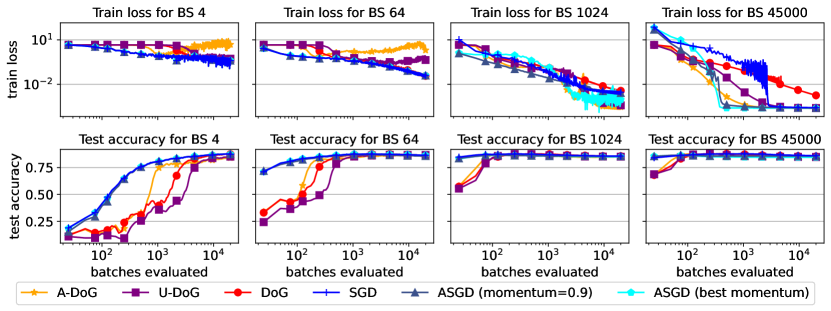
Figure 4: Training a linear model with ViT-32 features and log loss on CIFAR-100. Top: Train loss. Bottom: Test accuracy after iterate averaging. First column: Batch size scaling of complexity to reach target performance. Second column: Learning curves. Third column: ASGD performance at all learning rates and momenta, contrasted with DoG variants.

Figure 5: Training a linear model with ViT-32 features and log loss on CIFAR-100. Top: Loss vs. batches processed training for different batch sizes. Bottom: Test accuracy of averaged model vs. batches processed for different batch sizes.

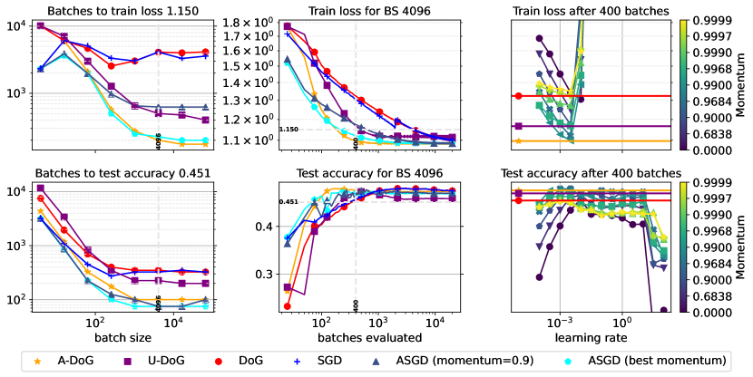
Figure 6: Training a linear model with ViT-32 features and log loss on DMLab. Top: Train loss. Bottom: Test accuracy after iterate averaging. First column: Batch size scaling of complexity to reach target performance. Second column: Learning curves. Third column: ASGD performance at all learning rates and momenta, contrasted with DoG variants.

Figure 7: Training a linear model with ViT-32 features and log loss on DMLab. Top: Loss vs. batches processed training for different batch sizes. Bottom: Test accuracy of averaged model vs. batches processed for different batch sizes.

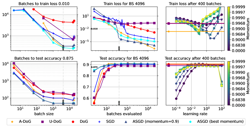
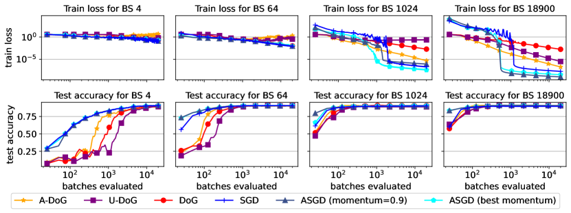
Figure 8: Training a linear model with ViT-32 features and log loss on Resisc45. Top: Train loss. Bottom: Test accuracy after iterate averaging. First column: Batch size scaling of complexity to reach target performance. Second column: Learning curves. Third column: ASGD performance at all learning rates and momenta, contrasted with DoG variants.

Figure 9: Training a linear model with ViT-32 features and log loss on Resisc45. Top: Loss vs. batches processed training for different batch sizes. Bottom: Test accuracy of averaged model vs. batches processed for different batch sizes.

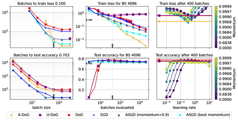
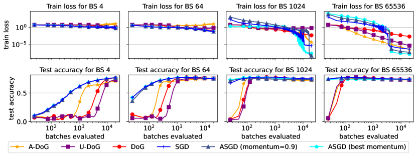
Figure 10: Training a linear model with ViT-32 features and log loss on Sun397. Top: Train loss. Bottom: Test accuracy after iterate averaging. First column: Batch size scaling of complexity to reach target performance. Second column: Learning curves. Third column: ASGD performance at all learning rates and momenta, contrasted with DoG variants.

Figure 11: Training a linear model with ViT-32 features and log loss on Sun397. Top: Loss vs. batches processed training for different batch sizes. Bottom: Test accuracy of averaged model vs. batches processed for different batch sizes.

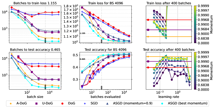
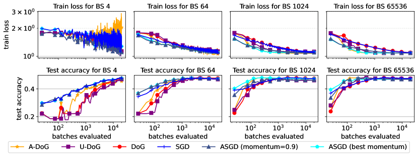
Figure 12: Training a linear model with ViT-32 features and log loss on CLEVR-Dist. Top: Train loss. Bottom: Test accuracy after iterate averaging. First column: Batch size scaling of complexity to reach target performance. Second column: Learning curves. Third column: ASGD performance at all learning rates and momenta, contrasted with DoG variants.

Figure 13: Training a linear model with ViT-32 features and log loss on CLEVR-Dist. Top: Loss vs. batches processed training for different batch sizes. Bottom: Test accuracy of averaged model vs. batches processed for different batch sizes.

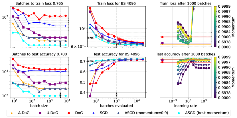
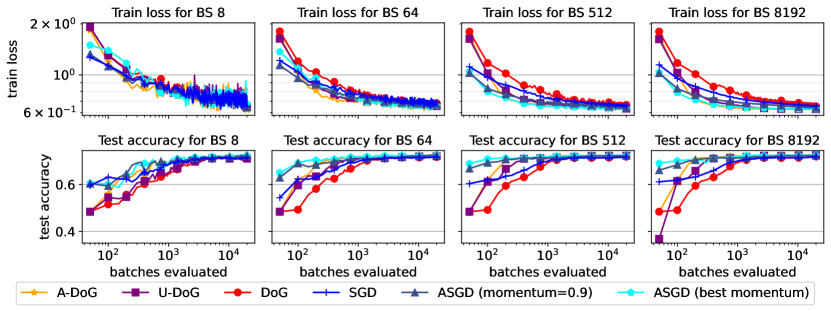
Figure 14: Training a linear model with log loss on LIBSVM/CovertypeScale. Top: Train loss. Bottom: Test accuracy after iterate averaging. First column: Batch size scaling of complexity to reach target performance. Second column: Learning curves. Third column: ASGD performance at all learning rates and momenta, contrasted with DoG variants.

Figure 15: Training a linear model with log loss on LIBSVM/CovertypeScale. Top: Loss vs. batches processed training for different batch sizes. Bottom: Test accuracy of averaged model vs. batches processed for different batch sizes.

We experiment with multi-class logistic regression on multiple tasks from the VTAB benchmark and the LIBSVM [10] suite (a full list is given in Section G.5). For VTAB tasks we use features obtained from a pretrained ViT-B/32 [18] model (i.e., perform linear probes), and for LIBSVM tasks we use apply logistic regression directly on the features provided. Figures 3, 5, 7, 9, 11, 13, 15 and 17 show a view of the results for different datasets analogous to Figure 1. Figures 3, 5, 7, 9, 11, 13, 15 and 17 give a complementary view by providing training curves at different batch sizes. As discussed in Section 5, we find that both U-DoG and A-DoG are competitive with well-tuned accelerated SGD (ASGD) and often significantly outperform DoG and tuned SGD. This is especially true for the training loss (for which our theory directly holds) and at large batch sizes, with A-DoG outperforming U-DoG in most cases, as both algorithms take advantage of the reduced variance in the gradient estimates to scale effectively with the batch size, as the theory suggests. In most experiments A-DoG attain and tuned ASGD attain superior convergence rate in terms of test accuracy as well as train loss; the only exception is CIFAR-100 (Figures 5 and 5, bottom rows) where the test accuracy does not closely track the train loss.

Least-squares.

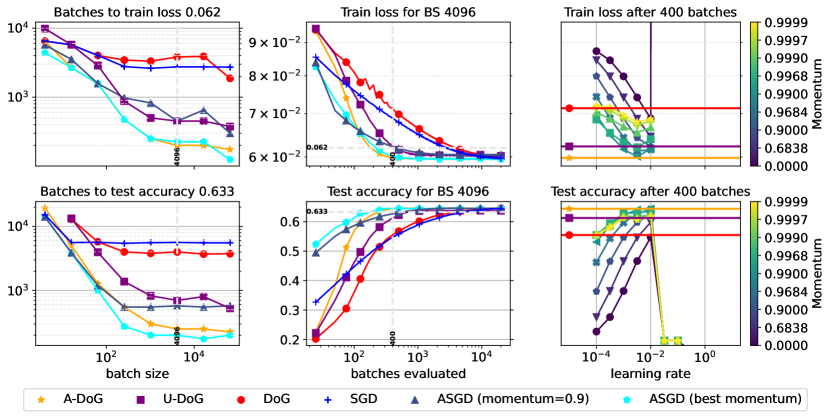
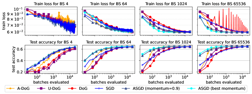
Figure 18: Training a linear model with ViT-32 features and least-squares loss on SVHN. Top: Train loss. Bottom: Test accuracy after iterate averaging. First column: Batch size scaling of complexity to reach target performance. Second column: Learning curves. Third column: ASGD performance at all learning rates and momenta, contrasted with DoG variants. This is the same as Figure 1.

Figure 19: Training a linear model with ResNet50 features and least-squares loss on SVHN. Top: Loss vs. batches processed training for different batch sizes. Bottom: Test accuracy of averaged model vs. batches processed for different batch sizes.

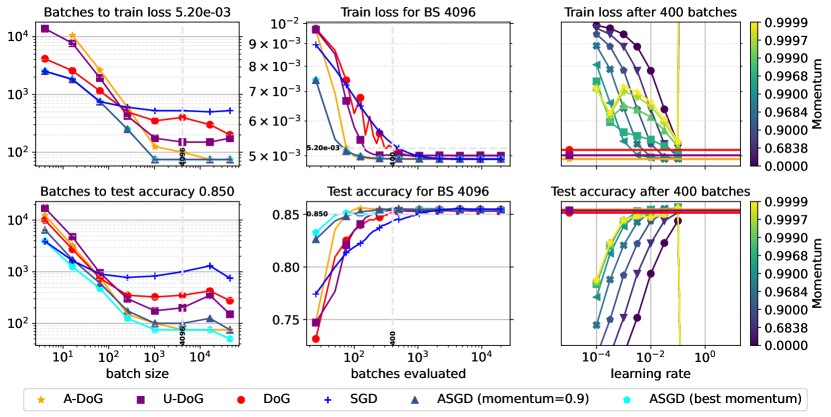
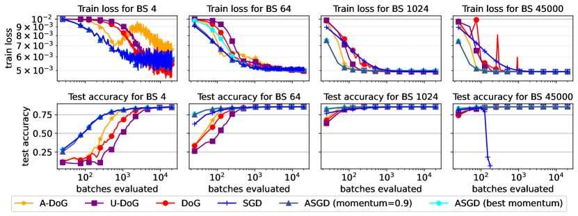
Figure 20: Training a linear model with ViT-32 features and least-squares loss on CIFAR-100. Top: Train loss. Bottom: Test accuracy after iterate averaging. First column: Batch size scaling of complexity to reach target performance. Second column: Learning curves. Third column: ASGD performance at all learning rates and momenta, contrasted with DoG variants.

Figure 21: Training a linear model with ResNet50 features and least-squares loss on CIFAR-100. Top: Loss vs. batches processed training for different batch sizes. Bottom: Test accuracy of averaged model vs. batches processed for different batch sizes.

We modify the loss on a subset of the previous experiments to least squares, learned over a one-hot encoding of the features. We use features obtained from a pretrained ViT-B/32, similar to what we used for the multiclass logistic regression. We find that our algorithms perform well in this setting as well. In comparison, while SGD and ASGD can perform well when tuned correctly, they become more sensitive to the choice of step size and momentum, performing poorly when not properly tuned and sometimes diverging completely. Similar to the other experiments, the results are given in Figures 19, 19, 21 and 21.

Noiseless quadratic experiments.

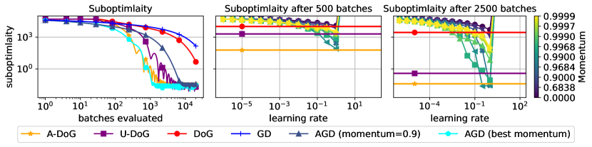
Figure 22: Training a model on a noiseless quadratic problem. At larger base learning rates, all AGD variants diverge while DoG variants remain stable, and U-DoG and A-DoG perform especially well.

As a final experiment, we compare the performance of the different algorithms on the quadratic function $f(x)=\sum_{i=1}^{n}\left(\frac{i}{2n}x_{i}^{2}+x_{i}\right)$ with $n=10^{4}$. The results agree with the theoretical analysis, with all algorithms reaching the optimal solution or very close to it, barring GD and AGD with excessively high momentum and learning rate. Results are depicted in Figure 22.

G.4 Non-convex experiments

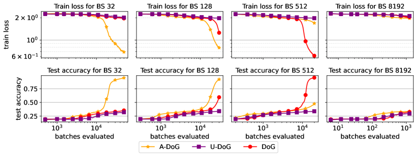
Figure 23: Training a ResNet50 model from scratch on SVHN. Top: Loss vs. batches processed training for different batch sizes. Bottom: Test accuracy vs. batches processed for averaged iterates at varied batch sizes.

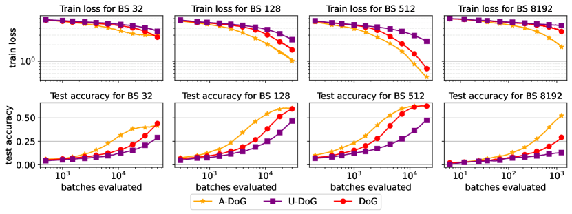
Figure 24: Training a ResNet50 model from scratch on Sun397. Top: Loss vs. batches processed training for different batch sizes. Bottom: Test accuracy vs. batches processed for averaged iterates at varied batch sizes.

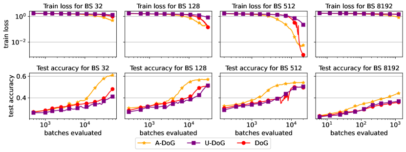
Figure 25: Training a ResNet50 model from scratch on DMLab. Top: Loss vs. batches processed training for different batch sizes. Bottom: Test accuracy vs. batches processed for averaged iterates at varied batch sizes.

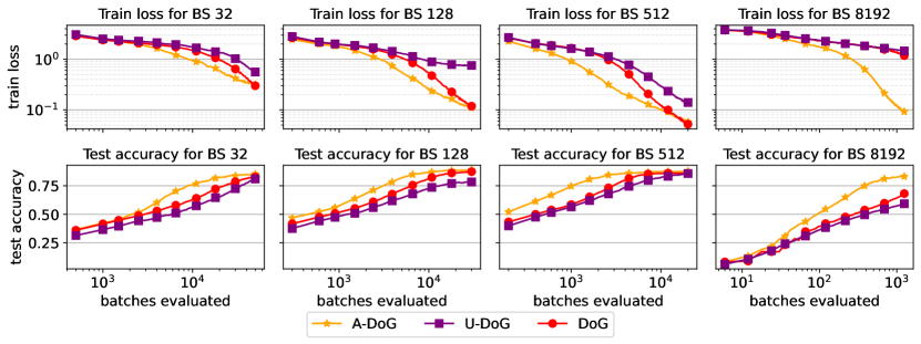
Figure 26: Training a ResNet50 model from scratch on Resisc45. Top: Loss vs. batches processed training for different batch sizes. Bottom: Test accuracy vs. batches processed for averaged iterates at varied batch sizes.

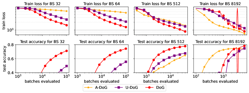
Figure 28: Fine-tuning a Clip-ViT-B/32 model on ImageNet, at different batch sizes. Top: Loss vs. step training curve for different batch sizes. Bottom: Test accuracy vs. step curve for averaged iterates at varied batch sizes.

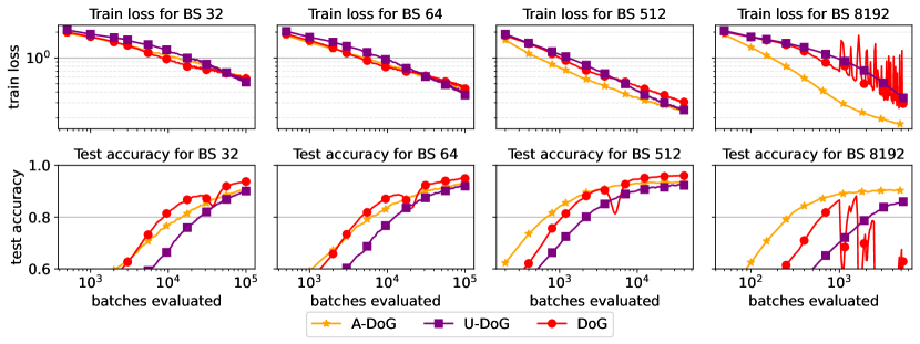
Figure 29: Training a Wide-ResNet-28-10 model on CIFAR-10 from scratch, at different batch sizes. Top: Loss vs. step training curve for different batch sizes. Bottom: Test accuracy vs. step curve for averaged iterates at varied batch sizes.

While we mainly focus on demonstrating the effectiveness of U-DoG and A-DoG in settings that match our theoretical analysis, we also perform preliminary experimentation in practical scenarios, namely training neural networks on datasets of moderate scales. In particular, we train a ResNet-50 [22] from scratch on a subset of the VTAB benchmark (Figures 23, 24, 25, 26 and 27). Additionally, we repeat two experiments from [25]: fine-tuning a CLIP model [50] on ImageNet (Figure 28), and training a WideResnet-28-10 [63] model from scratch on CIFAR-10 (Figure 29). We observe that U-DoG often fails to converge to competitive results, while A-DoG is quite competitive with DoG on the VTAB tasks, but under-performs it for CIFAR-10 and ImageNet fine-tuning, indicating that it is not a yet a viable general-purpose neural network optimizer.

G.5 Implementation details

Environment settings.

All of our experiments were based on PyTorch [48] (version 1.12.0). For DoG and the implementation of polynomial-decay model averaging [54], we used the the dog-optimizer package (version 1.0.3) [25]. For ASGD, we used the native PyTorch SGD with the Nesterov option enabled.

VTAB experiments were based on the PyTorch Image Models (timm, version0.7.0dev0) repository [60], with TensorFlow datasets (version 4.6.0) as a dataset backend [1]. LIBSVM [10] experiments were based on the libsvmdata (version 0.4.1) package.

To support the training and analysis of the results, we used numpy [21], scipy [58], pandas [59] and scikit-learn [49].

As much as possible, we leveraged existing recipes as provided by timm to train the models.

Datasets.

The subset of datasets used in our VTAB experiments are: CIFAR-100 [31], CLEVR-Dist [27], DMLab [4], Resisc45 [11], Sun397 [61, 62], and SVHN [43]. From LIBSVM, we used the Pendigits [2] and Covertype [7] datasets, where cover covertype we used the scaled features version (i.e., covtype.scale). We also experiment with CIFAR-10 [31] and ImageNet [16].

Models.

The computer vision pre-trained models were accessed via timm. The strings used to load the models were: ‘resnet50’, ‘vit_base_patch32_224_in21k’.

Complexity measure.

To fairly compare all algorithms, we measure complexity by the number of batches evaluated, i.e., the number of stochastic gradient queries performed by the algorithm. U-DoG requires two batches per iteration while the rest of the algorithms we consider require only one. We note that the algorithms we compare also have different memory footprints and runtimes per iteration (by constant factors). We focus on the number of batches as our complexity metric since it is most relevant to our theory. Memory and per-iteration runtime optimizations are potentially possible for U-DoG and A-DoG; we leave investigating those to future work.

ASGD model selection.

In the convex optimization experiments, we run (A)SGD over a wide range of momentum and learning rate parameters. For the batch size scaling figures (e.g., the left panels in Figure 1), we pick the parameters that reach the target metric in the smallest number of batches, providing a conservative upper bound on the performance obtainable with a very carefully tuned algorithm. The learning curve figures adjacent to the batch size scaling figures (e.g., the middle panels in Figure 1) show the learning curve for the (A)SGD run attaining the best target performance at the batch size indicated. For plots of learning curves at different batch sizes (e.g., Figure 19), we select the (A)SGD parameters that are the first to reach 95% of the best metric attained by A-DoG. If no such parameters exist, we take the parameters that reach the best performance within the iteration budget.

Iterate averaging.

When evaluating test accuracy, we follow Ivgi et al. [25] and apply polynomial-decay weight averaging [54] with parameter 8. We did not tune this parameter or comprehensively check how beneficial the averaging is. Nevertheless, a cursory examination of our data suggests that averaging is mostly helpful across the board, but much more so for DoG and SGD than their accelerated counterparts. This is in line with the theory, which provides guarantees on (essentially) the last iterate of U-DoG, but only the averaged iterate of DoG.

Learning rate schedule.

We use a constant learning rate schedule for (A)SGD. We do not use a decaying schedule such as cosine decay [34] as it would complicate comparing the smallest number of steps required to reach a target metric, since a decaying schedule requires knowing the number of steps in advance. Preliminary experiments indicate that, in the settings we study, cosine decay is not significantly better than a constant schedule combined with iterate averaging.

Setting $r_{\epsilon}$.

Similarly to Ivgi et al. [25] we set $r_{\epsilon}=\gamma\left(1+\|x_{0}\|\right)$ with $\gamma=10^{-6}$. Our theoretical analysis suggests that the particular choice of $r_{\epsilon}$ does not matter as long as it is sufficiently small relative to the distance between the weight initialization x0 and the optimum.

Weight decay.

We do not use weight decay in most experiments, except for training from scratch on CIFAR-10 (Figure 29), where we use a weight decay of $5\cdot 10^{-4}$. For DoG we decay the parameters toward zero, while for U-DoG and A-DoG we decay the parameters toward the initial point $x_{0}$. That is, for DoG we add $5\cdot 10^{-4}x$ to the stochastic gradient evaluated at $x$, while for U-DoG and A-DoG we add $5\cdot 10^{-4}(x-x_{0})$.

Gradient accumulation.

Due to GPU memory limitations, in the non-convex experiments, for large batch sizes we divide each batch into smaller sub-batches of size of either 128 or 256 samples. We calculate the gradient for each sub-batch and average those into a single gradient which we then use to perform a single step. When batch normalization is used (that is, for ResNet50), this is not mathematically identical to computing the gradient in one large batch.

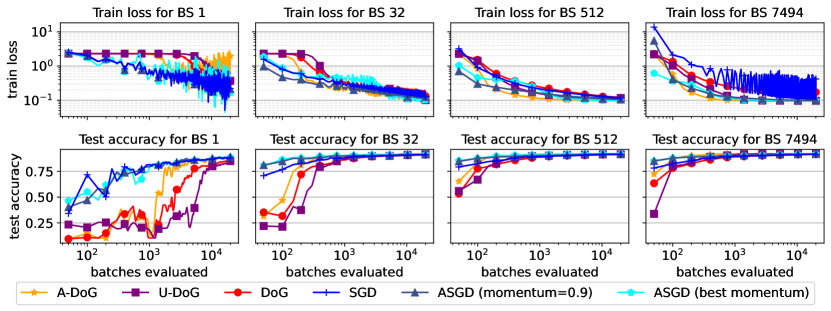
Figure 16: Training a linear model with log loss on LIBSVM/Pendigits. Top: Train loss. Bottom: Test accuracy after iterate averaging. First column: Batch size scaling of complexity to reach target performance. Second column: Learning curves. Third column: ASGD performance at all learning rates and momenta, contrasted with DoG variants.

Figure 17: Training a linear model with log loss on LIBSVM/Pendigits. Top: Loss vs. batches processed training for different batch sizes. Bottom: Test accuracy of averaged model vs. batches processed for different batch sizes. As most algorithms here fail to converge at reasonable rate, we use significantly lower targets to choose hyper-parameters.

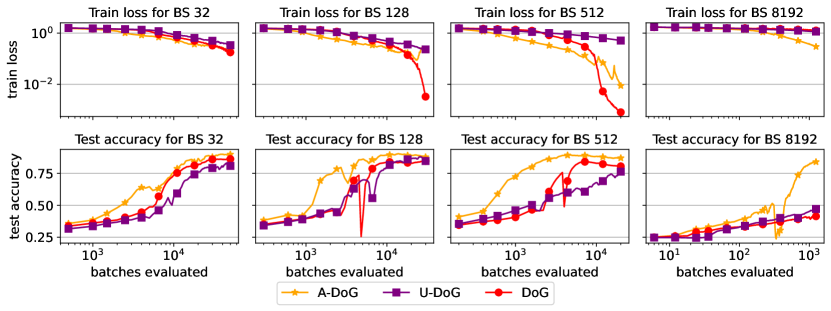
Figure 27: Training a ResNet50 model from scratch on CLEVR-Dist. Top: Loss vs. batches processed training for different batch sizes. Bottom: Test accuracy vs. batches processed for averaged iterates at varied batch sizes.

References

• Abadi et al. [2015] M. Abadi, A. Agarwal, P. Barham, E. Brevdo, Z. Chen, C. Citro, G. S. Corrado, A. Davis, J. Dean, M. Devin, S. Ghemawat, I. Goodfellow, A. Harp, G. Irving, M. Isard, Y. Jia, R. Jozefowicz, L. Kaiser, M. Kudlur, J. Levenberg, D. Mané, R. Monga, S. Moore, D. Murray, C. Olah, M. Schuster, J. Shlens, B. Steiner, I. Sutskever, K. Talwar, P. Tucker, V. Vanhoucke, V. Vasudevan, F. Viégas, O. Vinyals, P. Warden, M. Wattenberg, M. Wicke, Y. Yu, and X. Zheng. TensorFlow: Large-scale machine learning on heterogeneous systems, 2015.
• Alpaydin and Alimoglu [1998] E. Alpaydin and F. Alimoglu. Pen-Based Recognition of Handwritten Digits. UCI Machine Learning Repository, 1998. DOI: https://doi.org/10.24432/C5MG6K.
• Attia and Koren [2023] A. Attia and T. Koren. SGD with AdaGrad stepsizes: Full adaptivity with high probability to unknown parameters, unbounded gradients and affine variance. In International Conference on Machine Learning (ICML), 2023.
• Beattie et al. [2016] C. Beattie, J. Z. Leibo, D. Teplyashin, T. Ward, M. Wainwright, H. Küttler, A. Lefrancq, S. Green, V. Valdés, A. Sadik, et al. Deepmind lab. arXiv:1612.03801, 2016.
• Beck and Teboulle [2009] A. Beck and M. Teboulle. A fast iterative shrinkage-thresholding algorithm for linear inverse problems. SIAM journal on imaging sciences, 2(1):183–202, 2009.
• Bhaskara et al. [2020] A. Bhaskara, A. Cutkosky, R. Kumar, and M. Purohit. Online learning with imperfect hints. In International Conference on Machine Learning (ICML), 2020.
• Blackard [1998] J. Blackard. Covertype. UCI Machine Learning Repository, 1998. DOI: https://doi.org/10.24432/C50K5N.
• Carmon and Hinder [2022] Y. Carmon and O. Hinder. Making SGD parameter-free. In Conference on Learning Theory (COLT), 2022.
• Carmon et al. [2022] Y. Carmon, D. Hausler, A. Jambulapati, Y. Jin, and A. Sidford. Optimal and adaptive monteiro-svaiter acceleration. In Advances in Neural Information Processing Systems (NeurIPS), 2022.
• Chang and Lin [2011] C.-C. Chang and C.-J. Lin. LIBSVM: a library for support vector machines. ACM Transactions on Intelligent Systems and Technology, 2011.
• Cheng et al. [2017] G. Cheng, J. Han, and X. Lu. Remote sensing image scene classification: Benchmark and state of the art. Proceedings of the IEEE, 105(10):1865–1883, 2017.
• Cutkosky [2019a] A. Cutkosky. Anytime online-to-batch, optimism and acceleration. In International Conference on Machine Learning (ICML), pages 1446–1454, 2019a.
• Cutkosky [2019b] A. Cutkosky. Artificial constraints and hints for unbounded online learning. In Conference on Learning Theory (COLT), 2019b.
• Cutkosky and Orabona [2018] A. Cutkosky and F. Orabona. Black-box reductions for parameter-free online learning in Banach spaces. In Conference on Learning Theory (COLT), 2018.
• Defazio and Mishchenko [2023] A. Defazio and K. Mishchenko. Learning-rate-free learning by D-adaptation. In International Conference on Machine Learning (ICML), 2023.
• Deng et al. [2009] J. Deng, W. Dong, R. Socher, L.-J. Li, K. Li, and L. Fei-Fei. ImageNet: A large-scale hierarchical image database. In Conference on Computer Vision and Pattern Recognition (CVPR), 2009.
• Diakonikolas and Orecchia [2018] J. Diakonikolas and L. Orecchia. Accelerated extra-gradient descent: A novel accelerated first-order method. In Innovations in Theoretical Computer Science (ITCS), 2018.
• Dosovitskiy et al. [2021] A. Dosovitskiy, L. Beyer, A. Kolesnikov, D. Weissenborn, X. Zhai, T. Unterthiner, M. Dehghani, M. Minderer, G. Heigold, S. Gelly, J. Uszkoreit, and N. Houlsby. An image is worth 16x16 words: Transformers for image recognition at scale. In International Conference on Learning Representations (ICLR), 2021.
• Duchi et al. [2011] J. Duchi, E. Hazan, and Y. Singer. Adaptive subgradient methods for online learning and stochastic optimization. Journal of Machine Learning Research, 12(7), 2011.
• Gupta et al. [2017] V. Gupta, T. Koren, and Y. Singer. A unified approach to adaptive regularization in online and stochastic optimization. arXiv:1706.06569, 2017.
• Harris et al. [2020] C. R. Harris, K. J. Millman, S. J. van der Walt, R. Gommers, P. Virtanen, D. Cournapeau, E. Wieser, J. Taylor, S. Berg, N. J. Smith, R. Kern, M. Picus, S. Hoyer, M. H. van Kerkwijk, M. Brett, A. Haldane, J. F. del Río, M. Wiebe, P. Peterson, P. Gérard-Marchant, K. Sheppard, T. Reddy, W. Weckesser, H. Abbasi, C. Gohlke, and T. E. Oliphant. Array programming with NumPy. Nature, 585(7825):357–362, 2020.
• He et al. [2016] K. He, X. Zhang, S. Ren, and J. Sun. Deep residual learning for image recognition. Conference on Computer Vision and Pattern Recognition (CVPR), 2016.
• Howard et al. [2020] S. R. Howard, A. Ramdas, J. McAuliffe, and J. Sekhon. Time-uniform chernoff bounds via nonnegative supermartingales. Probability Surveys, 17:257–317, 2020.
• Howard et al. [2021] S. R. Howard, A. Ramdas, J. McAuliffe, and J. Sekhon. Time-uniform, nonparametric, nonasymptotic confidence sequences. The Annals of Statistics, 49(2):1055–1080, 2021.
• Ivgi et al. [2023] M. Ivgi, O. Hinder, and Y. Carmon. DoG is SGD’s best friend: A parameter-free dynamic step size schedule. In International Conference on Machine Learning (ICML), 2023. We refer to the latest arXiv version: https://arxiv.org/abs/2302.12022.
• Jacobsen and Cutkosky [2022] A. Jacobsen and A. Cutkosky. Parameter-free mirror descent. In Conference on Learning Theory (COLT), 2022.
• Johnson et al. [2017] J. Johnson, B. Hariharan, L. Van Der Maaten, L. Fei-Fei, C. Lawrence Zitnick, and R. Girshick. CLEVR: A diagnostic dataset for compositional language and elementary visual reasoning. In Conference on Computer Vision and Pattern Recognition (CVPR), 2017.
• Kavis et al. [2019] A. Kavis, K. Y. Levy, F. Bach, and V. Cevher. UniXGrad: A universal, adaptive algorithm with optimal guarantees for constrained optimization. Advances in Neural Information Processing Systems (NeurIPS), 2019.
• Khaled et al. [2023] A. Khaled, K. Mishchenko, and C. Jin. DoWG unleashed: An efficient universal parameter-free gradient descent method. In Advances in Neural Information Processing Systems (NeurIPS), 2023.
• Kingma and Ba [2015] D. P. Kingma and J. Ba. ADAM: A method for stochastic optimization. In International Conference on Learning Representations (ICLR), 2015.
• Krizhevsky [2009] A. Krizhevsky. Learning multiple layers of features from tiny images. Technical report, University of Toronto, 2009.
• Lan [2012] G. Lan. An optimal method for stochastic composite optimization. Mathematical Programming, 133(1):365–397, 2012.
• Levy et al. [2018] K. Y. Levy, A. Yurtsever, and V. Cevher. Online adaptive methods, universality and acceleration. Advances in Neural Information Processing Systems (NeurIPS), 2018.
• Loshchilov and Hutter [2017] I. Loshchilov and F. Hutter. SGDR: Stochastic gradient descent with warm restarts. International Conference on Learning Representations, 2017.
• McMahan [2017] H. B. McMahan. A survey of algorithms and analysis for adaptive online learning. The Journal of Machine Learning Research, 18(1):3117–3166, 2017.
• McMahan and Orabona [2014] H. B. McMahan and F. Orabona. Unconstrained online linear learning in Hilbert spaces: Minimax algorithms and normal approximations. In Conference on Learning Theory (COLT), 2014.
• McMahan and Streeter [2010] H. B. McMahan and M. Streeter. Adaptive bound optimization for online convex optimization. arXiv:1002.4908, 2010.
• Mhammedi and Koolen [2020] Z. Mhammedi and W. M. Koolen. Lipschitz and comparator-norm adaptivity in online learning. In Conference on Learning Theory (COLT), 2020.
• Mishchenko and Defazio [2023] K. Mishchenko and A. Defazio. Prodigy: An expeditiously adaptive parameter-free learner. arXiv:2306.06101, 2023.
• Nemirovski [2004] A. Nemirovski. Prox-method with rate of convergence $o(1/t)$ for variational inequalities with Lipschitz continuous monotone operators and smooth convex-concave saddle point problems. SIAM Journal on Optimization, 15(1):229–251, 2004.
• Nesterov [1983] Y. Nesterov. A method of solving a convex programming problem with convergence rate ${O}(1/k^{2})$. Soviet Mathematics Doklady, 27(2):372–376, 1983.
• Nesterov [2013] Y. Nesterov. Introductory Lectures on Convex Optimization: A Basic Course, volume 87. Springer Science & Business Media, 2013.
• Netzer et al. [2011] Y. Netzer, T. Wang, A. Coates, A. Bissacco, B. Wu, and A. Ng. Reading digits in natural images with unsupervised feature learning. In NIPS Workshop on Deep Learning and Unsupervised Feature Learning 2011, 2011.
• Orabona [2013] F. Orabona. Dimension-free exponentiated gradient. Advances in Neural Information Processing Systems (NeurIPS), 2013.
• Orabona [2021] F. Orabona. A modern introduction to online learning. arXiv:1912.13213, 2021.
• Orabona and Pál [2016] F. Orabona and D. Pál. Coin betting and parameter-free online learning. In Advances in Neural Information Processing Systems (NeurIPS), 2016.
• Paquette and Scheinberg [2020] C. Paquette and K. Scheinberg. A stochastic line search method with expected complexity analysis. SIAM Journal on Optimization, 30(1):349–376, 2020.
• Paszke et al. [2019] A. Paszke, S. Gross, F. Massa, A. Lerer, J. Bradbury, G. Chanan, T. Killeen, Z. Lin, N. Gimelshein, L. Antiga, A. Desmaison, A. Kopf, E. Yang, Z. DeVito, M. Raison, A. Tejani, S. Chilamkurthy, B. Steiner, L. Fang, J. Bai, and S. Chintala. PyTorch: An imperative style, high-performance deep learning library. In Advances in Neural Information Processing Systems (NeurIPS), 2019.
• Pedregosa et al. [2011] F. Pedregosa, G. Varoquaux, A. Gramfort, V. Michel, B. Thirion, O. Grisel, M. Blondel, P. Prettenhofer, R. Weiss, V. Dubourg, et al. Scikit-learn: Machine learning in Python. Journal of Machine Learning Research, 12:2825–2830, 2011.
• Radford et al. [2021] A. Radford, J. W. Kim, C. Hallacy, A. Ramesh, G. Goh, S. Agarwal, G. Sastry, A. Askell, P. Mishkin, J. Clark, et al. Learning transferable visual models from natural language supervision. In International Conference on Machine Learning (ICML), 2021.
• Rakhlin and Sridharan [2013] S. Rakhlin and K. Sridharan. Optimization, learning, and games with predictable sequences. In Advances in Neural Information Processing Systems (NeurIPS), 2013.
• Reddi et al. [2018] S. J. Reddi, S. Kale, and S. Kumar. On the convergence of Adam and beyond. In International Conference on Learning Representations (ICLR), 2018.
• Shallue et al. [2019] C. J. Shallue, J. Lee, J. Antognini, J. Sohl-Dickstein, R. Frostig, and G. E. Dahl. Measuring the effects of data parallelism neural network training. Journal of Machine Learning Research, 20:1–49, 2019.
• Shamir and Zhang [2013] O. Shamir and T. Zhang. Stochastic gradient descent for non-smooth optimization: Convergence results and optimal averaging schemes. In International Conference on Machine Learning (ICML), 2013.
• Shazeer and Stern [2018] N. Shazeer and M. Stern. Adafactor: Adaptive learning rates with sublinear memory cost. In International Conference on Machine Learning (ICML), 2018.
• Streeter and McMahan [2012] M. Streeter and H. B. McMahan. No-regret algorithms for unconstrained online convex optimization. In Advances in Neural Information Processing Systems (NeurIPS), 2012.
• Vaswani et al. [2019] S. Vaswani, A. Mishkin, I. Laradji, M. Schmidt, G. Gidel, and S. Lacoste-Julien. Painless stochastic gradient: Interpolation, line-search, and convergence rates. In Advances in Neural Information Processing Systems (NeurIPS), 2019.
• Virtanen et al. [2020] P. Virtanen, R. Gommers, T. E. Oliphant, M. Haberland, T. Reddy, D. Cournapeau, E. Burovski, P. Peterson, W. Weckesser, J. Bright, S. J. van der Walt, M. Brett, J. Wilson, K. J. Millman, N. Mayorov, A. R. J. Nelson, E. Jones, R. Kern, E. Larson, C. J. Carey, İ. Polat, Y. Feng, E. W. Moore, J. VanderPlas, D. Laxalde, J. Perktold, R. Cimrman, I. Henriksen, E. A. Quintero, C. R. Harris, A. M. Archibald, A. H. Ribeiro, F. Pedregosa, P. van Mulbregt, and SciPy 1.0 Contributors. SciPy 1.0: Fundamental Algorithms for Scientific Computing in Python. Nature Methods, 17:261–272, 2020.
• Wes McKinney [2010] Wes McKinney. Data Structures for Statistical Computing in Python. In Proceedings of the 9th Python in Science Conference, 2010.
• Wightman [2019] R. Wightman. PyTorch image models. https://github.com/rwightman/pytorch-image-models, 2019.
• Xiao et al. [2010] J. Xiao, J. Hays, K. A. Ehinger, A. Oliva, and A. Torralba. Sun database: Large-scale scene recognition from abbey to zoo. In Conference on Computer Vision and Pattern Recognition (CVPR), 2010.
• Xiao et al. [2016] J. Xiao, K. A. Ehinger, J. Hays, A. Torralba, and A. Oliva. Sun database: Exploring a large collection of scene categories. International Journal of Computer Vision, 119(1):3–22, 2016.
• Zagoruyko and Komodakis [2016] S. Zagoruyko and N. Komodakis. Wide residual networks. In British Machine Vision Conference (BMVC), 2016.
• Zhai et al. [2019] X. Zhai, J. Puigcerver, A. Kolesnikov, P. Ruyssen, C. Riquelme, M. Lucic, J. Djolonga, A. S. Pinto, M. Neumann, A. Dosovitskiy, L. Beyer, O. Bachem, M. Tschannen, M. Michalski, O. Bousquet, S. Gelly, and N. Houlsby. A large-scale study of representation learning with the visual task adaptation benchmark. arXiv:1910.04867, 2019.