[type=editor,orcid=0009-0007-9239-4092]
[1]
Conceptualisation, Investigation, Data curation, Formal Analysis, Software, Visualisation, Writing - original draft
1]organization=Department of Physics, addressline=University of Warwick, Gibbet Hill Road, city=Coventry, postcode=CV4 7AL, country=United Kingdom
[type=editor,orcid=0000-0002-8719-3313] \creditConceptualisation, Methodology, Writing - review & editing, Supervision
Real-space renormalisation approach to the Chalker-Coddington model revisited: improved statistics
Abstract
The real-space renormalisation group method can be applied to the Chalker-Coddington model of the quantum Hall transition to provide a convenient numerical estimation of the localisation critical exponent, . Previous such studies found which falls considerably short of the current best estimates by transfer matrix () and exact-diagonalisation studies (). By increasing the amount of data fold we can now measure closer to the critical point and find an improved estimate . This deviates only from the previous two values and is already better than the accuracy of the classical small-cell renormalisation approach from which our method is adapted. We also study a previously proposed mixing of the Chalker-Coddington model with a classical scattering model which is meant to provide a route to understanding why experimental estimates give a lower . Upon implementing this mixing into our RG unit, we find only further increases to the value of .
keywords:
Quantum Hall Effect \sepPhase Transition \sepLocalisation \sepCritical Exponent \sepRenormalisation \sepChalker-Coddington Model \sepReal-Space Renormalisation Group \sepGeometric DisorderWe measure the critical exponent of the quantum Hall transition, , ten times closer to the critical point by improving upon previous numerics with a fold increase in the number of data points.
We find an increased value of .
Our new value is just different from the current best numerical prediction based on large-scale transfer matrix computations.
1 Introduction
The plateau transitions of the quantum Hall effect (QHE) have retained interest over numerous decades [1, 2, 3, 4, 5, 6, 7, 8, 9, 10, 11, 12, 13, 14]. At least four reasons come to mind that might explain this continuing attention: (i) the QHE offers a fairly accessible approach, both theoretically and experimentally, to studying the interplay of many-body interactions and disorder, due to its low-dimensionality, its ready realization in well-understood semiconductor platforms and its by now fairly accommodating magnetic-field requirements [15, 16, 17, 18]. Next, (ii) the QHE exhibits the simplest of the topological phase transitions, serving both as a springboard into the field and a convenient benchmark case for the many advances in topological systems in the last decade [19, 20, 21, 22, 23, 24, 25]. Still, the QHE also retains some of its mysteries with (iii) ongoing interest in its microscopic mechanisms [26, 27, 28] and the importance of interactions in both integer and fractional QHEs [29, 30, 31, 32, 33, 34] and (iv) the remaining discrepancies between experimental measurements and theoretical predictions [35, 36, 37].
The precise value of the critical exponent governing the plateau-to-plateau transitions, even in the integer QHE, is a particularly intriguing such mystery [38]. While experimental results seem to have converged towards a value of [37], high-precision numerical studies have decisively shifted from earlier estimates, then in reasonable agreement with the experimental values, to a significantly higher value of [36, 39]. This later increase comes from three independent improvements, namely (1) studies with increased system sizes, allowing the analysis to move ever closer to the transition point, (2) better theoretical modelling of the behaviour close to the transition with a more convincing treatment of irrelevant finite-size corrections and (3) an improvement in the statistics of the generated data. A similar such improvement of experimental data, which could be achieved by (1) lowering experimental temperature and (2) better control of experimental parameters, has not yet been undertaken, but might lead to a similarly increasing exponent. Nevertheless, in the absence of improved experimental results one is drawn to evaluating other theoretical approaches. In a series of papers [40, 41], following on from [38], it was recently argued that a mix of classical and quantum networks can lead to a reduced estimate of to values again in agreement with experimental studies. Still, it remains unclear that such models can truly capture the QHE situation. Nevertheless, one should at least try and see if all the theoretical models formerly giving can now be shown to consistently give when (-) are followed.
This program is what we present here for the case of the real-space renormalisation group (RSRG) to the Chalker-Coddington (CC) network model of the integer QHE, a method judiciously adapted from a similar RSRG for classical percolation [42]. In the CC model, the method had previously been shown to give [43]. This is better than what should have been expected since the RSRG in the classical percolation only produces the critical exponent of the percolation transition within . As we will show here, by increasing the number of samples -fold, while also employing arbitrary-precision arithmetic [44], we now find a value of . In addition, we use the improved RSRG to also study the mixed problem of classical and quantum nodes proposed in [40, 38] mentioned above. Sadly, we find that the problem is very sensitive to the geometry of the chosen renormalisation group (RG) unit. While fixed point distributions can be constructed and estimates of critical exponents can be found, these do not readily correspond to known universality classes.
2 Real-Space Renormalisation Group on the Chalker-Coddington Model
2.1 Scattering matrix approach to the QH transition
The CC model describes the magnetic-field-induced chiral transport in the integer QHE via a 2D lattice populated with nodes representing saddle points in a continuous potential landscape. Electron wave packets can travel along directed equipotential paths – clockwise or counterclockwise according to the direction of the magnetic field – and scatter between such paths via tunelling across the saddlepoint nodes. Self-interference along the paths leads to localization while the tunnelling enhances electron transport. Taken together, the effects combine such that in summary the CC model exhibits a localisation-delocalisation-localisation transition at a single energy, hence modelling the plateau-to-plateau transitions of the QHE. The CC model has been previously employed in many studies of integer QHE physics [45, 35, 46, 47, 48, 49, 50]. In particular, when coupled with finite-size scaling, it can be used in transfer matrix studies to estimate the value of as discussed above [36].
Mathematically, each saddle point is represented by a matrix connecting two incoming, , with two outgoing channels, , as . Charge conservation is expressed via unitarity such that with representing a hermitian conjugate. The most general complex-valued matrix obeying these constraints is
| (1) |
with , , the complex conjugate and a phase. Popular choices are
| (2) |
Here, , refer to transmission and reflection amplitudes in the first representation with [51] while the latter uses a single mixing angle, [3].
With reference to the potential landscape, an effective saddle point height, , can be defined by [52]
| (3) |
In the following, we shall denote the distribution of these parameters over all saddle points as , and . A further parameter, of perhaps more direct experimental relevance, is the dimensionless conductance with . Furthermore, and .
2.2 RG determination of the fixed point distributions at the QH transition
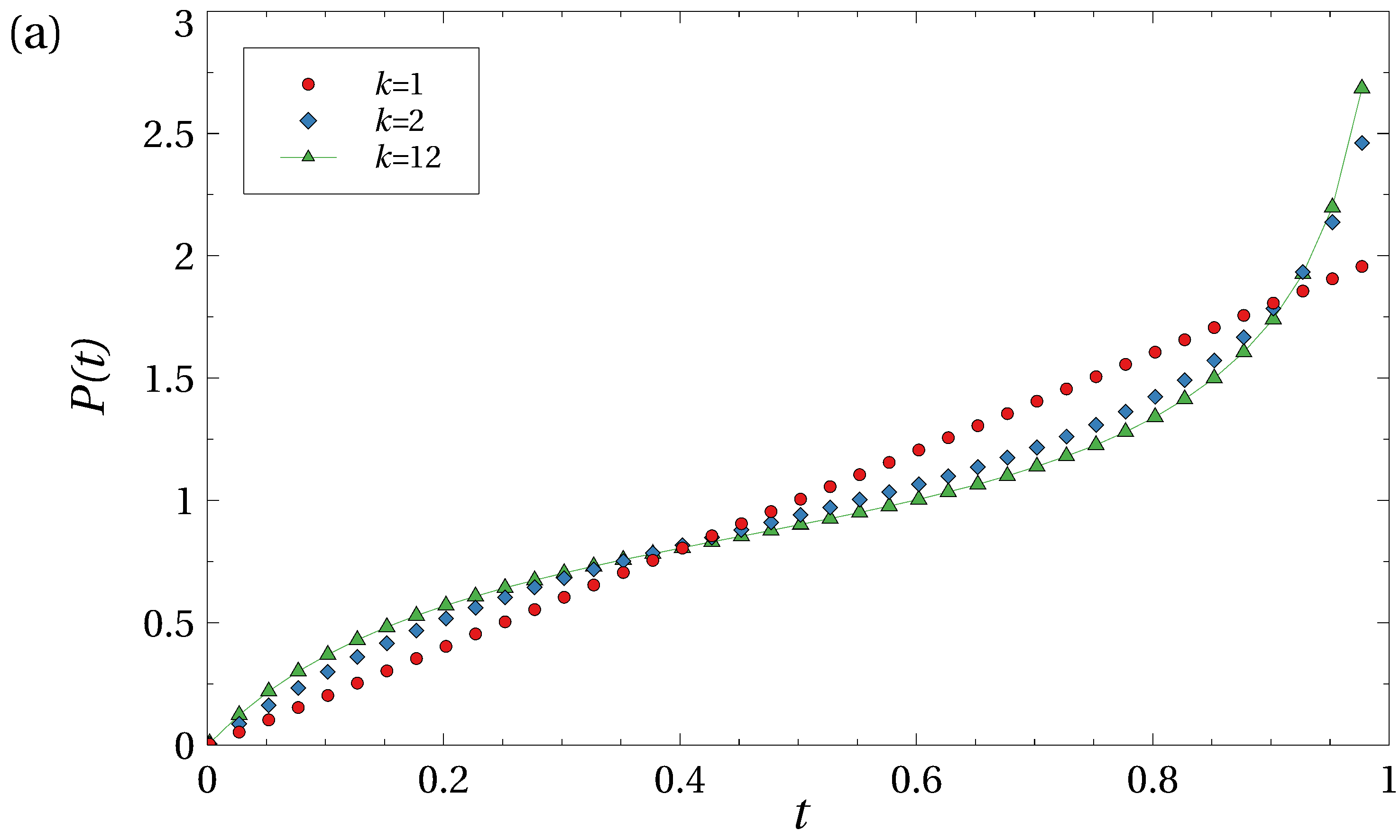
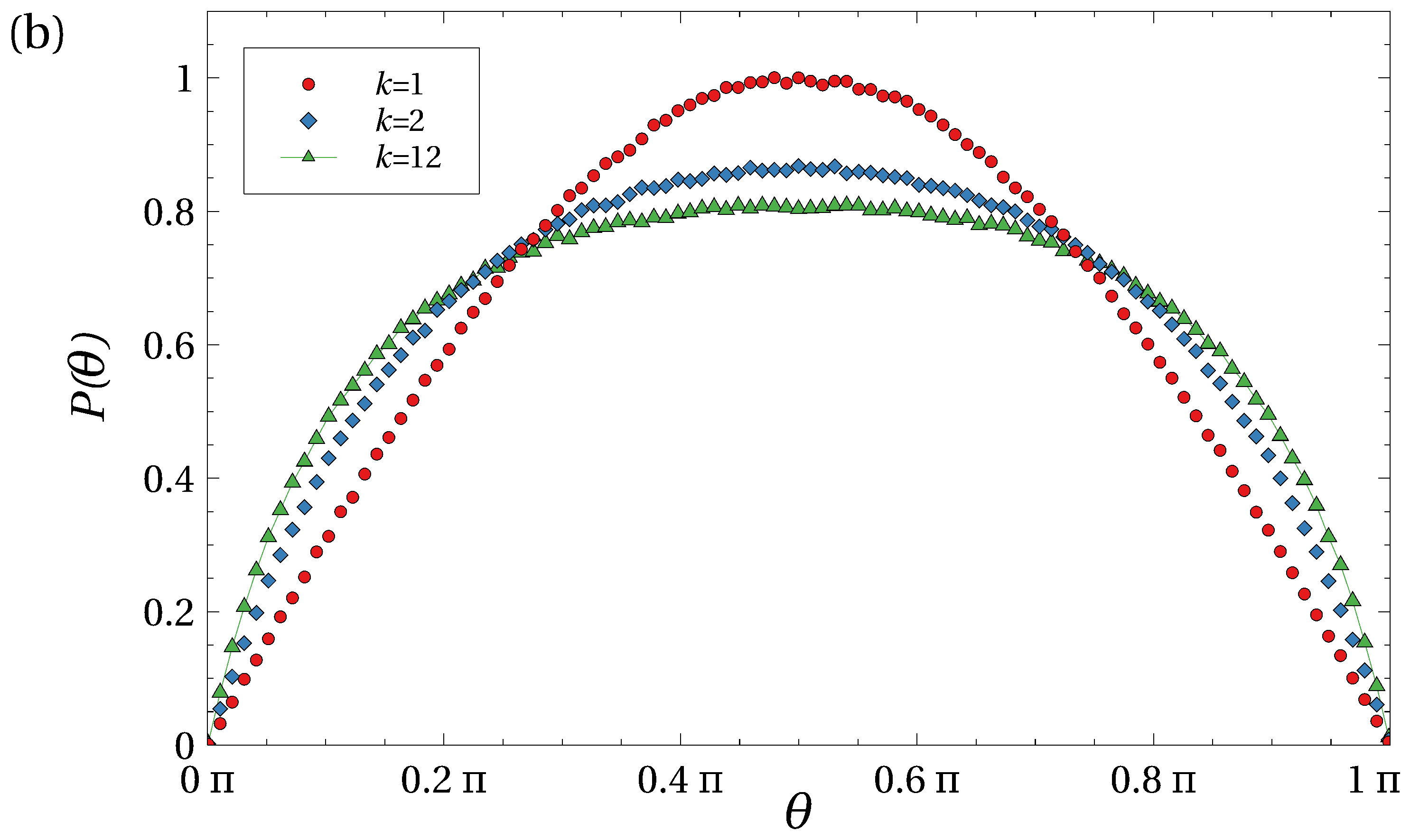
Transfer matrix and diagonalization studies of the CC model usually build up quasi-1D strips or 2D square lattices of saddle points and then proceed to compute localization lengths, participation numbers, etc. [53, 54]. The RSRG approach, on the other hand, works by considering a small subset of such a lattice structure by constructing an RG unit from several neighbouring nodes [52]. For the RG unit, we assemble the matrices of each participating node into a combined matrix and remove all unwanted connections to superfluous in- and outgoing channels such that we are only left with again two incoming and two outgoing channels. In figure 1, we show this RG unit graphically. We note that other RG units are possible, but none have thus far been shown to yield better results [55, 43] than the -node RG unit depicted in figure 1. We emphasize that in drawing the figure, we have used the fact that the phases along the four closed loops add. The five matrices combine into a single matrix equation, previously shown in Refs. [43, 55] in the , representation. Using , we find equation 4. In principle, starting with the five saddle points described by mixing angles , and the phases of the four closed loops , we can compute the effective mixing angle of the super-saddle point.
We are now ready to proceed with the RG process itself. We first need to construct a starting distribution of parameters. Then application of the RG for RG generations will allow us to find the distribution of super-parameters [52]. At criticality, we expect that for with denoting the unstable fixed point (FP) distribution [43].111Starting from a distribution too asymmetric or to far away from the , the RG flow will tend towards the stable classical FPs, e.g. or .
While this procedure can in principle be done using any of the , , or representations, here we choose a combination of and representations for convenience [51]. We start with , equivalent to (and ), and generate . The phases are chosen randomly in to model spatial variation among equipotentials. {strip}
| (4) |
We then transform each value to and find . Cain et al. [51] have shown that the approach to the fixed point results in a sequence of symmetric distributions such that with . Conversely, the symmetry can be enforced for each and a symmetrized with constructed following the transformation relations given at the end of section 2.1. This stabilizes the approach to the fixed point distributions , , etc.
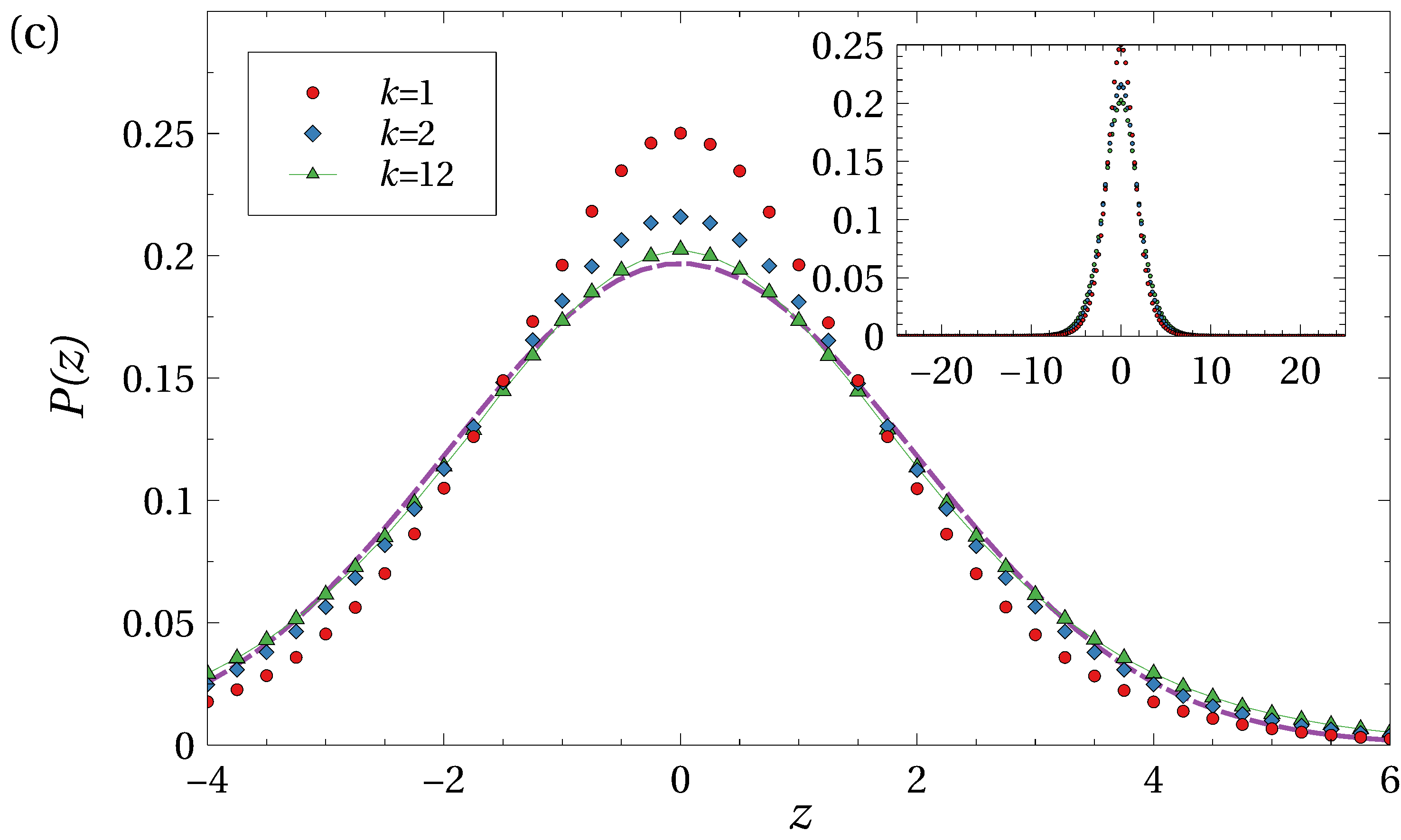

We implement this procedure and generate at least values for each RG generation . This is about times more than in previous such RG studies [56]. Since the generated super-distributions will be no longer comprised of simple functions, we employ the rejection method [57] to generate appropriate random numbers. Also, in the version implemented for this work, we use Mathematica’s arbitrary-precision arithmetic when evaluating Eq. (4) (in the representation [51]). This reduces inevitable rounding errors when computing and values with usual compiler-based double precision arithmetic, allowing us to keep accurate track of values ranging from ( to (.
In figure 2, we show the resulting FP distributions for (a) , (b) , (c) and (d) . We note that the spread of around reflects the distribution of the disorder landscape. A fit to a Gaussian for can be obtained via a usual minimization taking into account the uncertainties of the values. However, a perfect fit is only achieved when we increase the uncertainties -fold. Nevertheless, the coefficient of determination is with and standard deviation . The fitted Gaussian curve is shown alongside the data in Figure 2(c). We conclude that a Gaussian approximation is suitable, in particular for determining the maximum value of successive distributions with a restricted range, and we use it below in determining the mean shift in saddle point heights.
2.3 Determination of an improved critical exponent
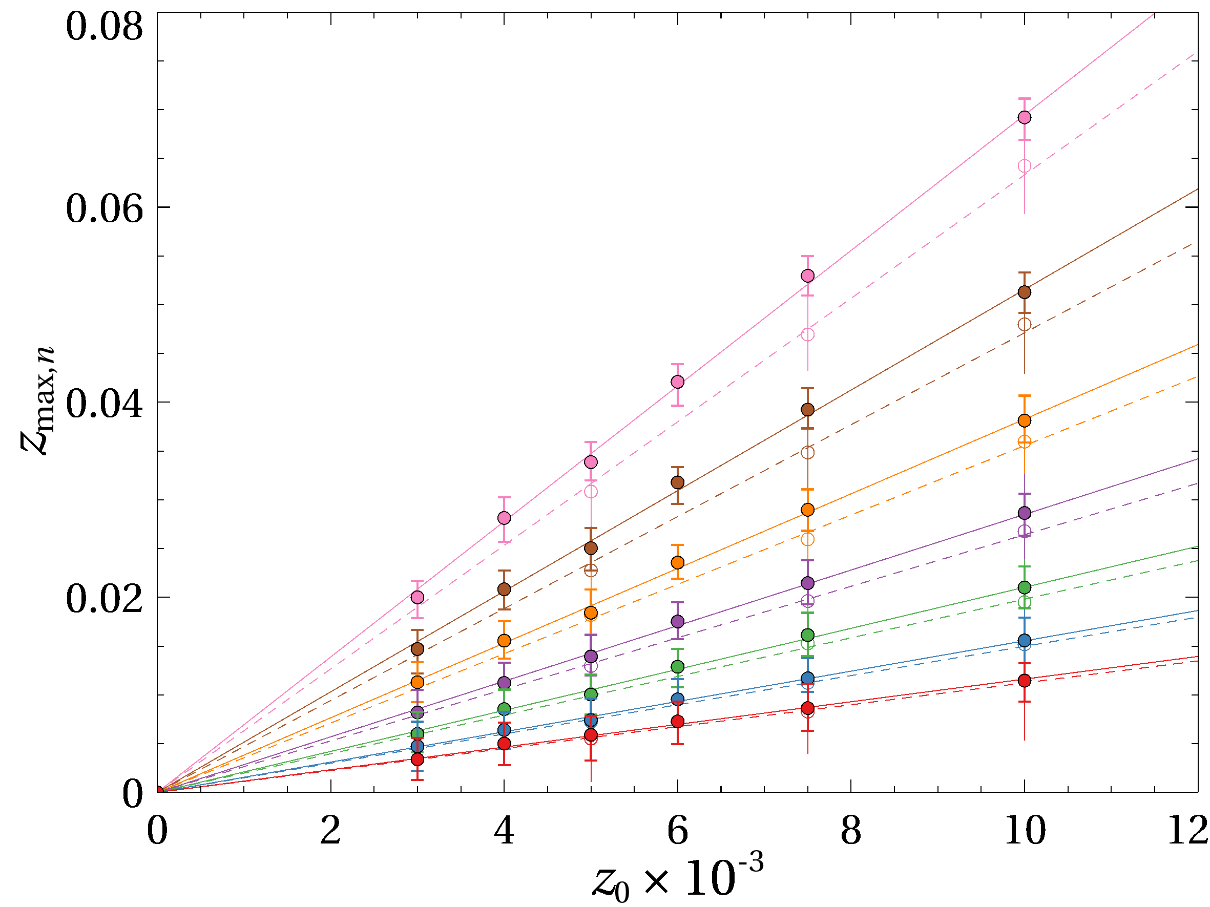
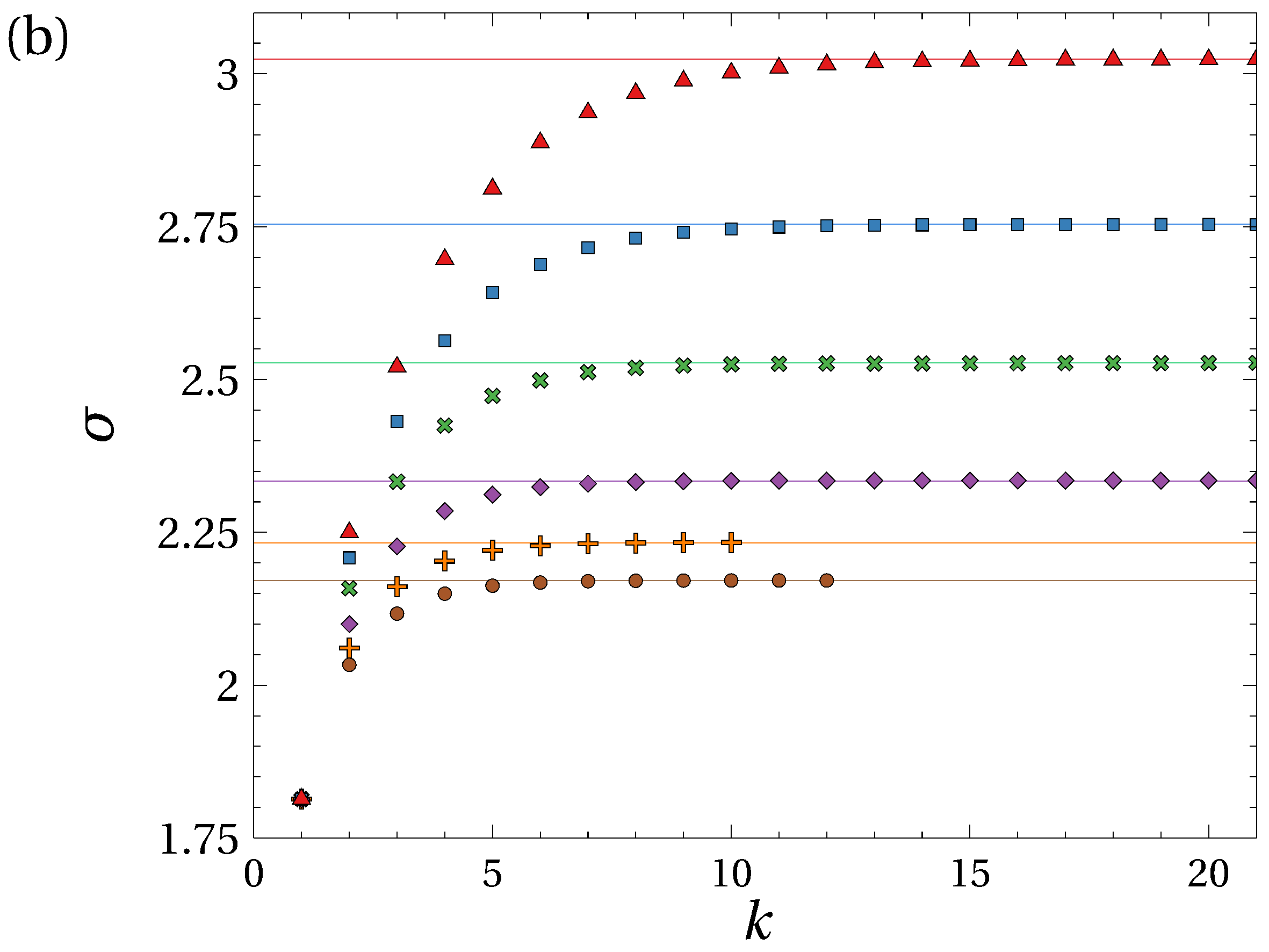
To determine the critical exponent , we next perturb the FP distribution by a constant shift , i.e. . We then observe how the perturbed distribution drifts away from criticality by monitoring the deviation of its maximum at from under repeated (unsymmetrized) RG steps [51]. Only the largest of values, corresponding approximately to all , are used to determine by fitting to a Gaussian as shown in figure 3.
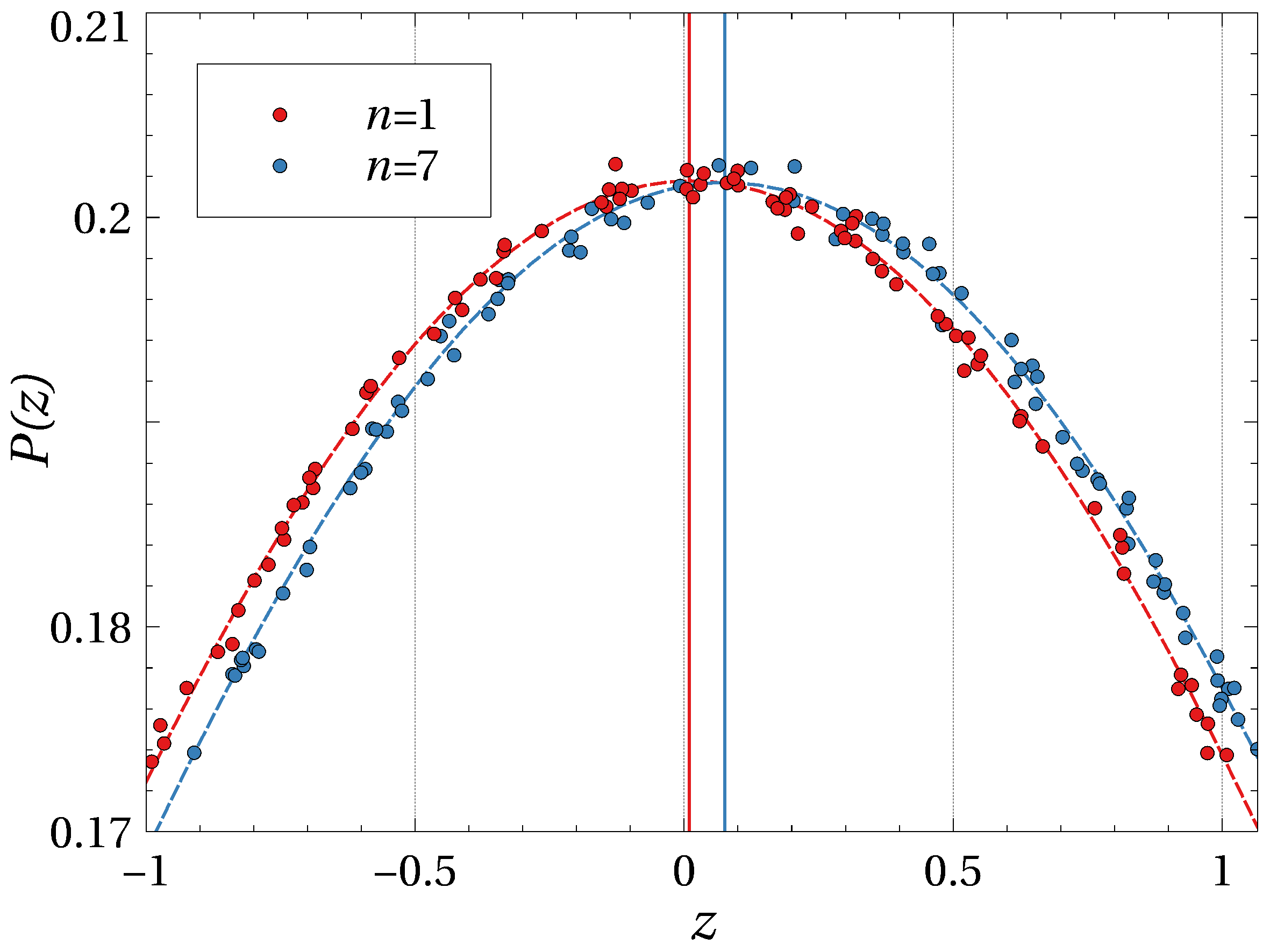
After such RG steps, we find that the position of the maximum follows with good accuracy as detailed in figure 4.
The critical exponent can then be computed via [52]
| (5) |
and should converge for . As presented in figure 5, we find for .
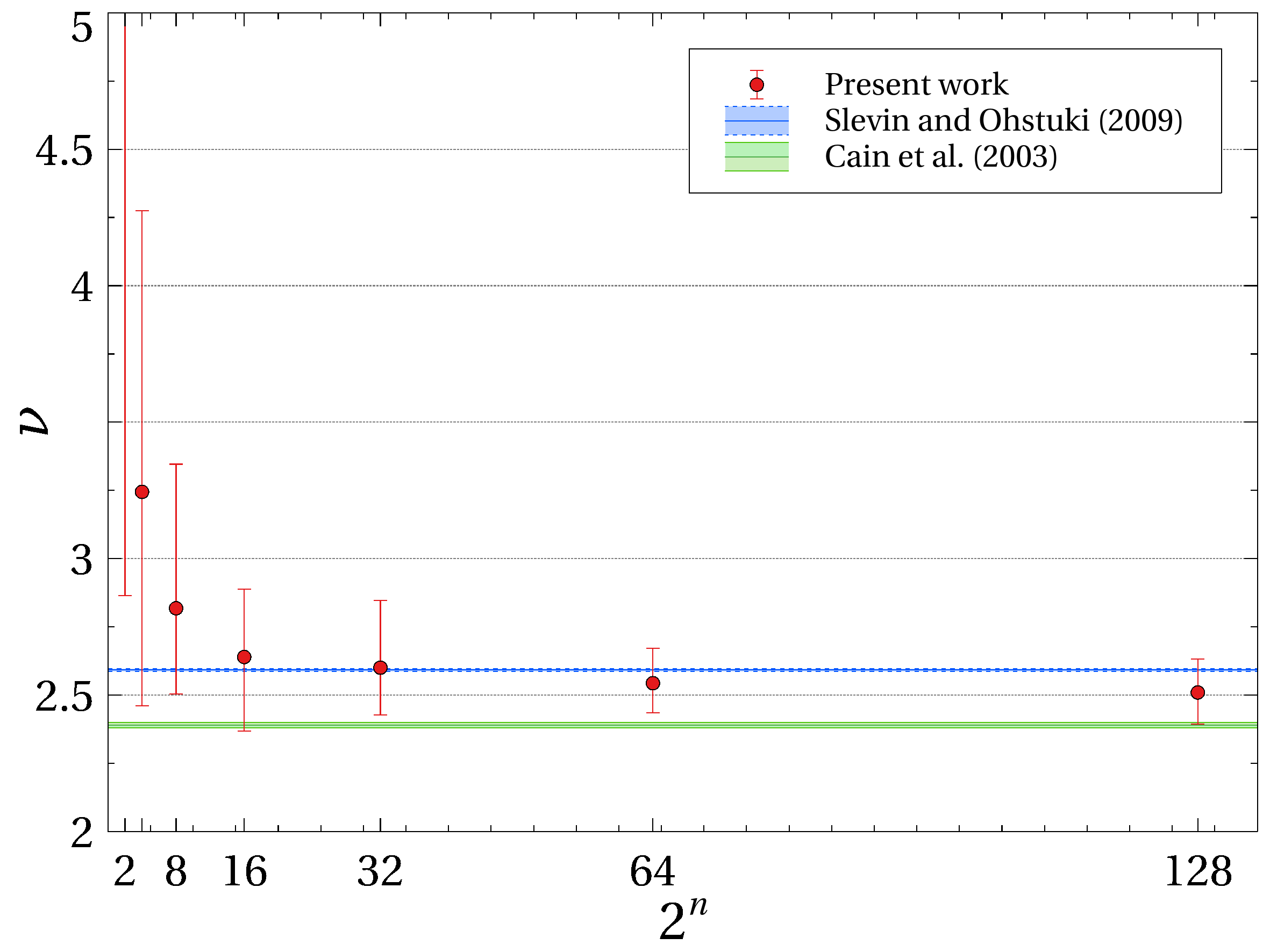
In obtaining this increased value, the enhanced statistics of allows us to study initial perturbations , and . These values are ten times smaller than used previously, hence increasing the accuracy of the determination for . With the accepted value from transfer matrix calculations [36], we find that our new result only deviates by . This is of course very good when compared to the accuracy in classical percolation [42].
3 Mixing classical and quantum percolation
While our new is now in better agreement with the high-precision estimates of Slevin and Ohtsuki [36] and Puschmann et al. [39], we have similarly increased the distance to the lower experimental estimates [37, 11]. Work by Nuding et al. [60] and others [38, 40] argues that this discrepancy could lie in the highly irregular arrangement of experimental scattering nodes which is nevertheless modelled on a square lattice in the CC model. They suggest that a mixed model, in which some nodes are left in the CC configuration, with and values, while other nodes are chosen fully open (, ) or fully closed (, ) with probability , could lower the value of to be in better agreement with the experiments.
3.1 Fixed point distributions for the mixed model
This type of mixed disorder, termed "geometric disorder" by Gruzberg et al. [38], can be implemented into the RSRG method by intentionally modifying values of the saddle points within the distributions. For distinction from the previous situation, we shall denote the resulting distributions as , , etc. With this notation, . Upon every th RG transformation each saddle point in the RG unit cell becomes, with probability , either entirely transmitting () or entirely reflecting (). Or, with probability , , the saddle point transmission amplitude remains a random number selected from the previous distribution , as before. But simply setting values to (i.e. ) in the analytic equation determining the renormalised (i.e. Eq. (4)) can result in a vanishing denominator. In terms of , the and values correspond to , respectively. Hence we see a build-up of large values in , which is increasing as increases. Clearly, if we were to use such distributions in our RG procedure, we would effectively double-count the influx of the mixed disorder [55]. We avoid this by neglecting all accumulated values beyond when computing in each RG step. Overall, the proportion of such events, , remains less than as we try to approach a new .
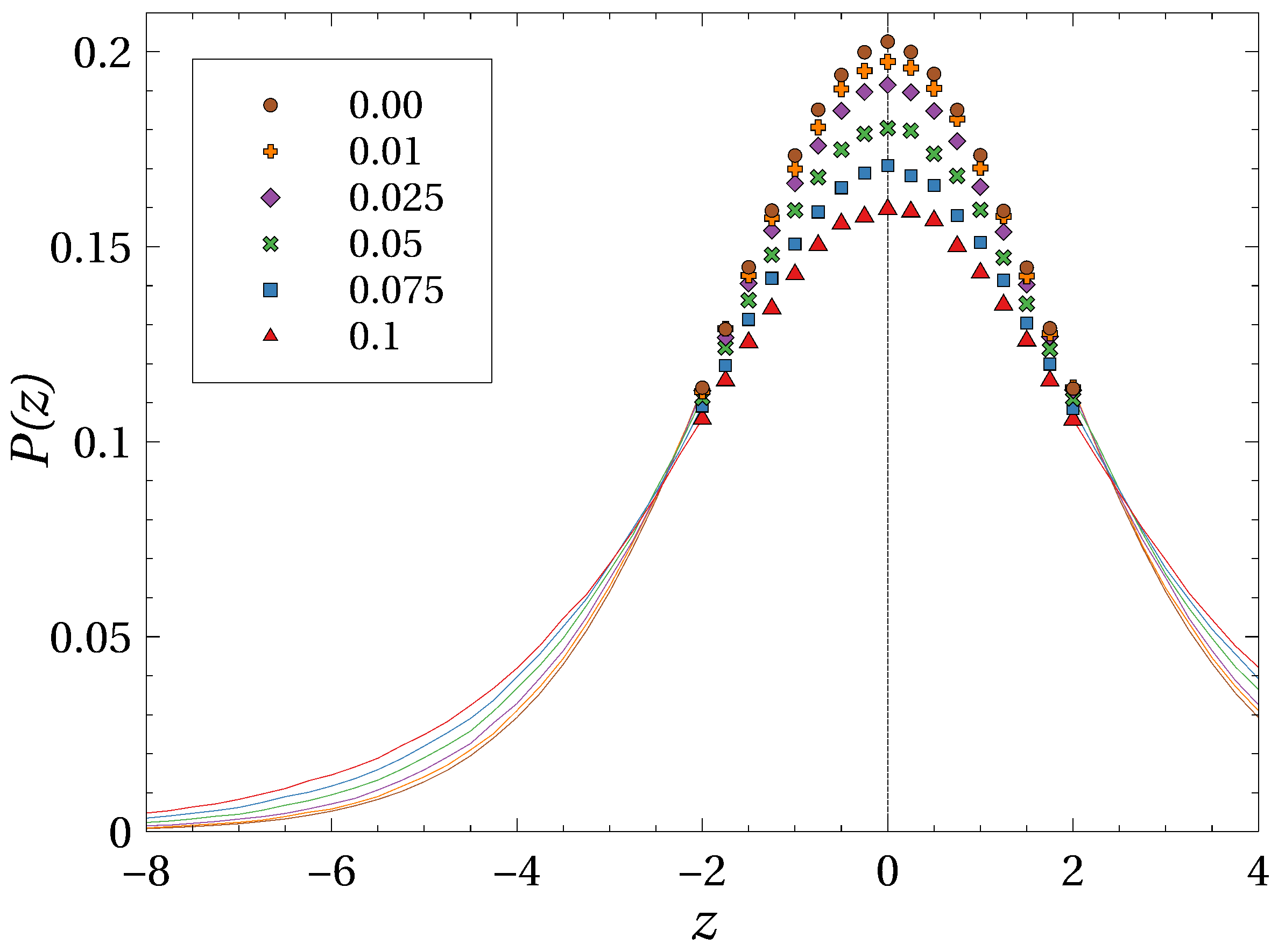
In figure 6 we show that we can indeed find this new FP distribution for the case of mixed disorder for various values. The fixed point distributions are again of roughly Gaussian shape with (e.g.) and () for , , , , , respectively, where denotes the number of bins used in constructing the distributions. In relation to , we note that the height-to-width ratio of is about times that of . The fixed point distributions with have significantly longer -tails, corresponding to a more rugged saddle point height landscape.
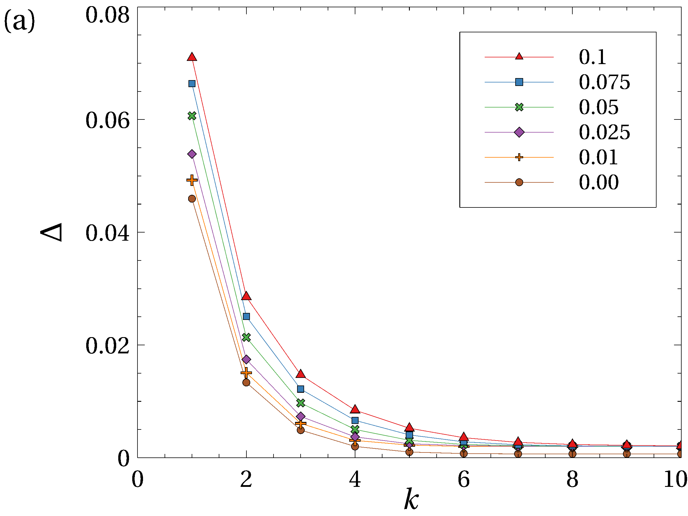
The introduction of mixed disorder has no effect on the mean value of the distribution, as random application of mixed disorder doesn’t bias the effective saddle point heights in either direction. However, the introduction of notably increases the amount of steps required to converge towards an FP distribution. This is shown in figure 7 with plotted against RG iteration number for varying values of . Additionally, the shape of the FP distribution changes depending on , as shown by the change in standard deviation converged upon for different values also in figure 7. For larger , we note a consistent increase in for each .
3.2 Critical exponent for the mixed model
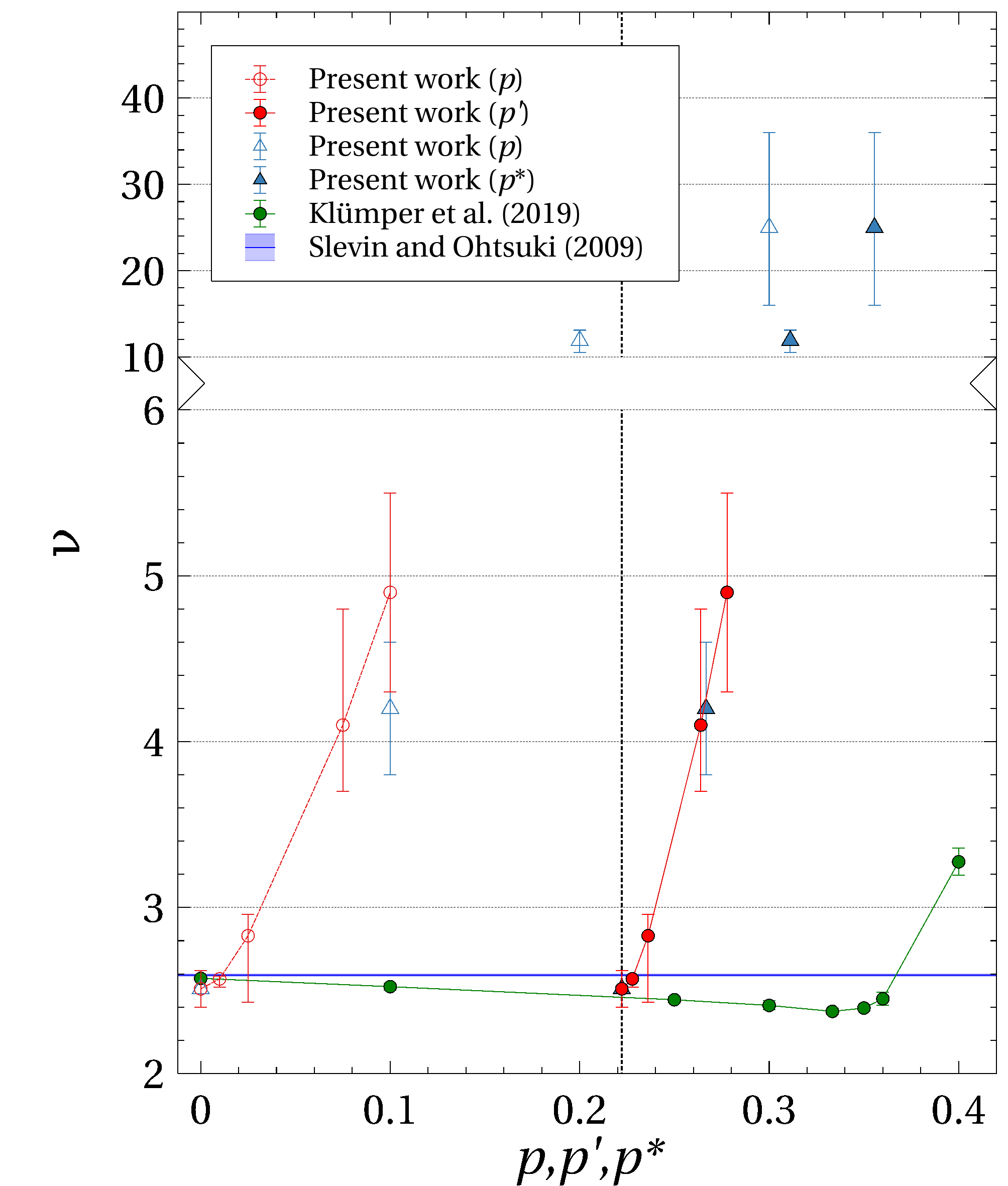
After having determined the FP distributions , we shift these as before by a small to determine the RG flow of the position on the maxima . As indicated in figure 4, we find good linearity and can hence proceed to determine, for each , a corresponding critical exponent of the mixed model, via equation (5). The results are astounding: the values of increase monotonically from to as shown in Table 1. Particularly the last number seems to indicate a behaviour at the QHE plateau-plateau transitions not found experimentally [59]. An increased value of up to was indeed observed in Klümper et al. [40]. But the overall quantitative agreement of our results with these previous results across all remains poor as shown in figure 8.
We find in particular that the agreement as a function of is unsatisfactory. When considering the structure of the RG unit in figure 1, we note that the four corner nodes had been chosen to correspond to and in the opposing corners of the RG unit. So instead of simply ignoring these four corner nodes and concentrating on the five-node RG unit, it would be equally justified to include them into a now nine-node RG unit in which the four corner nodes are already part of the mixed model. This then suggests that one might introduce a normalized with the in the initial expression chosen such that also. In figure 8, we show the results for . Clearly, is now in better agreement with the value of Klümper et al. [40]. But for other values, large differences remain.
Another source of systematic deviation from these results might be the small size of the RG unit and in particular, the privileged position of the central node, i.e. node three in figure 1. Effectively, it is the tunneling across this node which allows for self-interference in a figure-of-eight arrangement [52]. In our implementation of the mixed model, we have thus far allowed this node to also "percolate" with and . Excluding this possibility requires to rescale via such that . Our numerical results for both with and without this modification are displayed in table 1. The modification results in even larger values for than previously, as shown in figure 8. Clearly, we seem stuck in a situation where the RG approach cannot reproduce the results of the mixed model.
| 0 | 0.222 | ||
| 0.01 | 0.228 | ||
| 0.025 | 0.236 | ||
| 0.075 | 0.263 | ||
| 0.1 | 0.278 | ||
| 0.1 | 0.267 | ||
| 0.2 | 0.311 | ||
| 0.3 | 0.356 |
4 Conclusion
The localisation length critical exponent, , of the quantum Hall transition can be estimated with the RSRG applied to the Chalker-Coddington model. Increasing the number of the statistical sample sizes 500 times, and using a more precise model for numerical data, has allowed us to get more stable and reliable estimates for . This in turn has enabled us to study the RSRG description of closer to the fixed point, being able to reduce by a factor of ten when compared to earlier RSRG approaches [58]. We find an increased estimate of . This is in line with the general trend observed in the past - decades when studying critical properties of second-order (quantum) phase transitions: substantially better statistics coupled with larger system sizes shift critical exponents towards larger values. This is true for the exponent of the QHE [36, 39] as well as the 3D exponent of the Anderson metal-insulator transition [61, 62, 63]. A recent proposal for a deformed Wess-Zumino-Novikov-Witten type conformal field theoretic description of the QHE implies a resulting critical exponent [46], which would call for truly challenging computational resources or novel insight to allow a numerical validation.
For the mixed disorder model, proposed in reference [38], our results are inconclusive. Clearly, the model has its charms and attractions when discussed in connection to experimental results for the QHE. However, our current, very local RSRG cell fails to capture the expected behaviour of and returns rather unphysical results. Previous attempts to improve upon this by enlarging the RG cell have been shown to fail due to the inherent difficulties associated with such an approach [55].
5 Acknowledgments
We thank Warwick’s Scientific Computing Research Technology Platform for further computing time and support. UK research data statement: Data accompanying this publication are available at [64] while the code is at [65].
References
- von Klitzing et al. [2020] K. von Klitzing, T. Chakraborty, P. Kim, V. Madhavan, X. Dai, J. McIver, Y. Tokura, L. Savary, D. Smirnova, A. M. Rey, C. Felser, J. Gooth, X. Qi, 40 years of the quantum Hall effect, Nature Reviews Physics 2 (2020) 397–401.
- Girvin and Yang [2019] S. M. Girvin, K. Yang, Modern Condensed Matter Physics, Cambridge University Press, 2019. doi:10.1017/9781316480649.
- Son and Raghu [2021] J. H. Son, S. Raghu, Three-dimensional network model for strong topological insulator transitions, Physical Review B 104 (2021) 125142.
- Minkov and Savona [2016] M. Minkov, V. Savona, Haldane quantum Hall effect for light in a dynamically modulated array of resonators, Optica 3 (2016) 200.
- Ohgushi et al. [2000] K. Ohgushi, S. Murakami, N. Nagaosa, Spin anisotropy and quantum Hall effect in the kagomé lattice: Chiral spin state based on a ferromagnet, Physical Review B 62 (2000) R6065–R6068.
- Haldane [1988] F. D. M. Haldane, Model for a Quantum Hall Effect without Landau Levels: Condensed-Matter Realization of the "Parity Anomaly", Physical Review Letters 61 (1988) 2015–2018.
- Raghu and Haldane [2008] S. Raghu, F. D. M. Haldane, Analogs of quantum-Hall-effect edge states in photonic crystals, Physical Review A 78 (2008) 033834.
- Laughlin [1981] R. B. Laughlin, Quantized Hall conductivity in two dimensions, Physical Review B 23 (1981) 5632–5633.
- Tang et al. [2019] F. Tang, Y. Ren, P. Wang, R. Zhong, J. Schneeloch, S. A. Yang, K. Yang, P. A. Lee, G. Gu, Z. Qiao, L. Zhang, Three-dimensional quantum Hall effect and metal–insulator transition in ZrTe5, Nature 569 (2019) 537–541.
- Hannahs et al. [1989] S. T. Hannahs, J. S. Brooks, W. Kang, L. Y. Chiang, P. M. Chaikin, Quantum Hall effect in a bulk crystal, Physical Review Letters 63 (1989) 1988–1991.
- Hohls et al. [2002] F. Hohls, U. Zeitler, R. J. Haug, R. Meisels, K. Dybko, F. Kuchar, Dynamical Scaling of the Quantum Hall Plateau Transition Physical Review Letters 89(2002) 276801.
- Hashimoto et al. [2008] K. Hashimoto, C. Sohrmann, J. Wiebe, T. Inaoka, F. Meier, Y. Hirayama, R. A. Römer, R. Wiesendanger, M. Morgenstern, Quantum Hall Transition in Real Space: From Localized to Extended States, Physical Review Letters 101 (2008) 256802.
- d’Ambrumenil et al. [2011] N. d’Ambrumenil, B. I. Halperin, R. H. Morf, Model for dissipative conductance in fractional quantum Hall states, Physical Review Letters 106 (2011) 126804.
- Hashimoto et al. [2012] K. Hashimoto, T. Champel, S. Florens, C. Sohrmann, J. Wiebe, Y. Hirayama, R. A. Römer, R. Wiesendanger, M. Morgenstern, Robust Nodal Structure of Landau Level Wave Functions Revealed by Fourier Transform Scanning Tunneling Spectroscopy, Physical Review Letters 109 (2012) 116805.
- Parmentier et al. [2016] F. D. Parmentier, T. Cazimajou, Y. Sekine, H. Hibino, H. Irie, D. C. Glattli, N. Kumada, P. Roulleau, Quantum Hall effect in epitaxial graphene with permanent magnets, Scientific Reports 6 (2016) 38393.
- Novoselov et al. [2007] K. S. Novoselov, Z. Jiang, Y. Zhang, S. V. Morozov, H. L. Stormer, U. Zeitler, J. C. Maan, G. S. Boebinger, P. Kim, A. K. Geim, Room-Temperature Quantum Hall Effect in Graphene, Science 315 (2007) 1379–1379.
- Cao et al. [2012] H. Cao, J. Tian, I. Miotkowski, T. Shen, J. Hu, S. Qiao, Y. P. Chen, Quantized Hall Effect and Shubnikov–de Haas Oscillations in Highly Doped Bi2Se3 : Evidence for Layered Transport of Bulk Carriers, Physical Review Letters 108 (2012) 216803.
- Hill et al. [1998] S. Hill, S. Uji, M. Takashita, C. Terakura, T. Terashima, H. Aoki, J. S. Brooks, Z. Fisk, J. Sarrao, Bulk quantum Hall effect in eta-Mo4O11, Physical Review B 58 (1998) 10778–10783.
- Bernevig et al. [2006] B. A. Bernevig, T. L. Hughes, S.-C. Zhang, Quantum Spin Hall Effect and Topological Phase Transition in HgTe Quantum Wells, Science 314 (2006) 1757–1761.
- Hasan and Kane [2010] M. Z. Hasan, C. L. Kane, Topological insulators, Reviews of Modern Physics 82 (2010) 3045–3067.
- Qi et al. [2008] X. L. Qi, T. L. Hughes, S. C. Zhang, Topological field theory of time-reversal invariant insulators, Physical Review B - Condensed Matter and Materials Physics 78 (2008).
- Bernevig B A and Hughes T L [2013] Bernevig B A, Hughes T L, Topological Insulators and Topological Superconductors, Princeton University Press, 2013.
- Rachel [2018] S. Rachel, Interacting topological insulators: a review, Reports on Progress in Physics 81 (2018) 116501.
- Ozawa et al. [2019] T. Ozawa, H. M. Price, A. Amo, N. Goldman, M. Hafezi, L. Lu, M. C. Rechtsman, D. Schuster, J. Simon, O. Zilberberg, I. Carusotto, Topological photonics, Reviews of Modern Physics 91 (2019) 015006.
- Ding et al. [2022] K. Ding, C. Fang, G. Ma, Non-Hermitian topology and exceptional-point geometries, Nature Reviews Physics 4 (2022) 745–760.
- Ilani et al. [2004] S. Ilani, J. Martin, E. Teitelbaum, J. H. Smet, D. Mahalu, V. Umansky, A. Yacoby, The microscopic nature of localization in the quantum Hall effect, Nature 427 (2004) 328–332.
- Römer and Oswald [2021] R. A. Römer, J. Oswald, The microscopic picture of the integer quantum Hall regime, Annals of Physics 435 (2021) 168541.
- Weis and von Klitzing [2011] J. Weis, K. von Klitzing, Metrology and microscopic picture of the integer quantum Hall effect, Philosophical Transactions of the Royal Society A: Mathematical, Physical and Engineering Sciences 369 (2011) 3954–3974.
- Oswald [2023] J. Oswald, Revision of the edge channel picture for the integer quantum Hall effect, Results in Physics 47 (2023) 106381.
- Chklovskii et al. [1992] D. B. Chklovskii, B. I. Shklovskii, L. I. Glazman, Electrostatics of Edge Channels, Physical Review B 46 (1992) 4026–4034.
- Cooper and Chalker [1993] N. R. Cooper, J. T. Chalker, Coulomb interactions and the integer quantum Hall effect: Screening and transport, Physical Review B 48 (1993) 4530–4544.
- Oswald and Römer [2017a] J. Oswald, R. A. Römer, Manifestation of many-body interactions in the integer quantum Hall effect regime, Physical Review B 96 (2017a) 125128.
- Oswald and Römer [2017b] J. Oswald, R. A. Römer, Exchange-mediated dynamic screening in the integer quantum Hall effect regime, EPL (Europhysics Letters) 117 (2017b) 57009.
- Halperin and Jain [2020] B. I. Halperin, J. K. Jain, Fractional Quantum Hall Effects (2020).
- Kramer et al. [2005] B. Kramer, T. Ohtsuki, S. Kettemann, Random network models and quantum phase transitions in two dimensions, Physics Reports 417 (2005) 211-342.
- Slevin and Ohtsuki [2009] K. Slevin, T. Ohtsuki, Critical exponent for the quantum Hall transition, Physical Review B - Condensed Matter and Materials Physics 80 (2009).
- Li et al. [2009] W. Li, C. L. Vicente, J. S. Xia, W. Pan, D. C. Tsui, L. N. Pfeiffer, K. W. West, Scaling in plateau-to-plateau transition: A direct connection of quantum Hall systems with the Anderson localization model, Physical Review Letters 102 (2009).
- Gruzberg et al. [2017] I. A. Gruzberg, A. Klümper, W. Nuding, A. Sedrakyan, Geometrically disordered network models, quenched quantum gravity, and critical behavior at quantum Hall plateau transitions, Physical Review B 95 (2017) 125414.
- Puschmann et al. [2019] M. Puschmann, P. Cain, M. Schreiber, T. Vojta, Integer quantum Hall transition on a tight-binding lattice, Physical Review B 99 (2019) 121301.
- Klümper et al. [2019] A. Klümper, W. Nuding, A. Sedrakyan, Random network models with variable disorder of geometry, Physical Review B 100 (2019) 140201.
- Conti et al. [2021] R. Conti, H. Topchyan, R. Tateo, A. Sedrakyan, Geometry of random potentials: Induction of two-dimensional gravity in quantum Hall plateau transitions, Physical Review B 103 (2021).
- Stauffer and Aharony [1991] D. Stauffer, A. Aharony, Introduction to Percolation Theory, 2nd editio ed., Taylor & Francis Group, 1991.
- Cain and Römer [2005] P. Cain, R. A. Römer, Real-space renormalization-group approach to the integer quantum Hall effect, International Journal of Modern Physics B 19 (2005) 2085–2119.
- Wolfram Research [2022] Wolfram Research, Inc., Mathematica V13.x, Champaign, IL, 2022-2024.
- Chalker and Coddington [1988] J. T. Chalker, P. D. Coddington, Percolation, quantum tunnelling and the integer Hall effect, Journal of Physics C: Solid State Physics 21 (1988) 2665–2679.
- Zirnbauer [2021] M. R. Zirnbauer, Marginal CFT perturbations at the integer quantum Hall transition, Annals of Physics 431 (2021) 168559.
- Sedrakyan [2003] A. Sedrakyan, Action formulation of the network model of plateau-plateau transitions in the quantum Hall effect, Physical Review B 68 (2003) 235329.
- Chalker and Daniell [1988] J. T. Chalker, G. J. Daniell, Scaling, Diffusion, and the Integer Quantized Hall Effect, Physical Review Letters 61 (1988) 593–596.
- Kramer et al. [2003] B. Kramer, S. Kettemann, T. Ohtsuki, Localization in the quantum Hall regime, Physica E: Low-dimensional Systems and Nanostructures 20 (2003) 172–187.
- Evers and Brenig [1998] F. Evers, W. Brenig, Semiclassical theory of the quantum Hall effect, Physical Review B 57 (1998) 1805–1813.
- Cain et al. [2001] P. Cain, R. A. Römer, M. Schreiber, M. E. Raikh, Integer quantum Hall transition in the presence of a long-range-correlated quenched disorder, Physical Review B 64 (2001) 235326.
- Galstyan and Raikh [1997] A. G. Galstyan, M. E. Raikh, Localization and conductance fluctuations in the integer quantum Hall effect: Real-space renormalization-group approach, Physical Review B 56 (1997).
- Lee et al. [1993] D.-H. Lee, Z. Wang, S. Kivelson, Quantum percolation and plateau transitions in the quantum Hall effect, Physical Review Letters 70 (1993) 4130–4133.
- L Schweitzer et al. [1984] L Schweitzer, B Kramer, A MacKinnon, Magnetic field and electron states in two-dimensional disordered systems, Journal of Physics C: Solid State Physics 17 (1984) 4111–4125.
- Assi [2019] B. Assi, A Study of the Integer Quantum Hall Effect with a Modified Chalker-Coddington Network Model that Incorporates Geometric Disorder, Ph.D. thesis, University of Warwick, 2019.
- Cain et al. [2003] P. Cain, M. E. Raikh, R. A. Römer, Real-Space Renormalization Group Approach to the Quantum Hall Transition, Journal of the Physical Society of Japan 72 (2003) 135–136.
- Press et al. [2007] W. H. Press, S. A. Teukolsky, W. T. Vetterling, B. P. Flannery, Numerical recipes: the art of scientific computing, Cambridge University Press, 2007.
- Cain et al. [2003] P. Cain, R. A. Römer, M. E. Raikh, R. A. Römer, Renormalization group approach to the energy level statistics at the integer quantum Hall transition, Physica E: Low-dimensional Systems and Nanostructures 18 (2003) 126–127.
- Koch et al. [1991] S. Koch, R. J. Haug, K. von Klitzing, K. Ploog, Experiments on scaling in AlxGa1-xAs/GaAs heterostructures under quantum Hall conditions, Physical Review B 43 (1991) 6828–6831
- Nuding et al. [2015] W. Nuding, A. Klümper, A. Sedrakyan, Localization length index and subleading corrections in a Chalker-Coddington model: A numerical study, Physical Review B 91 (2015) 115107.
- Slevin and Ohtsuki [1999] K. Slevin, T. Ohtsuki, Corrections to Scaling at the Anderson Transition, Physical Review Letters 82 (1999) 382–385.
- Rodriguez et al. [2010] A. Rodriguez, L. J. Vasquez, K. Slevin, R. A. Römer, Critical Parameters from a Generalized Multifractal Analysis at the Anderson Transition, Physical Review Letters 105 (2010) 046403.
- Rodriguez et al. [2011] A. Rodriguez, L. J. Vasquez, K. Slevin, R. A. Römer, Multifractal finite-size scaling and universality at the Anderson transition, Physical Review B 84 (2011) 134209.
- Shaw and Romer [????] S. Shaw, R. A. Römer, Real-space renormalisation approach to the Chalker-Coddington model revisited: improved statistics, WRAP: Warwick Research Archive Portal, University of Warwick, URL: https://wrap.warwick.ac.uk/xxxxxx/.
- Shaw and Roemer [????] S. Shaw, R. A. Römer, DisQS/CCxD: Codes to simulate the real-space RG in variants of the Chalker-Coddington models, GitHub repository for the Disordered Quantum Systems Group, University of Warwick, URL: https://github.com/DisQS/CCxD.