Harmonic chain driven by active Rubin bath: transport properties and steady-state correlations
Abstract
Characterizing the properties of an extended system driven by active reservoirs is a question of increasing importance. Here we address this question in two steps. We start by investigating the dynamics of a probe particle connected to an ‘active Rubin bath’—a linear chain of overdamped run-and-tumble particles. We derive exact analytical expressions for the effective noise and dissipation kernels, acting on the probe, and show that the active nature of the bath leads to a modified fluctuation-dissipation relation. In the next step, we study the properties of an activity-driven system, modeled by a chain of harmonic oscillators connected to two such active reservoirs at the two ends. We show that the system reaches a nonequilibrium stationary state (NESS), remarkably different from that generated due to a thermal gradient. We characterize this NESS by computing the kinetic temperature profile, spatial and temporal velocity correlations of the oscillators, and the average energy current flowing through the system. It turns out that, the activity drive leads to the emergence of two characteristic length scales, proportional to the activities of the reservoirs. Strong signatures of activity are also manifest in the anomalous short-time decay of the velocity autocorrelations. Finally, we find that the energy current shows a non-monotonic dependence on the activity drive and reversal in direction, corroborating previous findings.
I Introduction
Nonequilibrium reservoirs, defying the fluctuation-dissipation relation (FDR) [1], show more complex behavior compared to their equilibrium counterparts [2, 3, 4, 5, 6]. Recent years have seen an increasing effort to model and characterize various kinds of nonequilibrium reservoirs. Active reservoirs refer to a special class of out-of-equilibrium reservoirs, which consist of a collection of self-propelled ‘active’ agents. Examples of active agents range from microorganisms like bacteria, and macroscopic living entities like birds to artificially synthesized Janus particles and nanobots. The self-propelled nature of active particles leads to a range of intriguing features for systems coupled to active reservoirs— examples include the emergence of negative friction, modification of equipartition theorem, anomalous relaxation dynamics, an algebraic behavior of the force-correlation, reduction of the efficiency of a Brownian Stirling engine, the emergence of short-range interaction, spontaneous rectification of chaotic motion, and linear scaling of diffusivity with activity [7, 8, 9, 10, 11, 12, 13, 14, 15].
A particularly important question is, how the nonequilibrium stationary state of an extended system is affected when driven by such active reservoirs. This question has recently been addressed in the context of energy transport through a harmonic chain, using a very simple model of an active reservoir[16, 17]. In these works, the effect of an active reservoir on a probe particle was modeled phenomenologically by introducing an ‘active’ self-propulsion force, in addition to the usual dissipative and white-noise forces coming from an equilibrium thermal reservoir. This simple model showed several intriguing features of the NESS including negative differential conductivity and a non-trivial directional reversal of the active current. It was also shown that this current-carrying NESS cannot be generated in a system driven by thermal reservoirs with activity-dependent effective temperatures, despite having an activity-dependent local kinetic temperature in the bulk. In this model, the active noise kernel is taken to be independent of the dissipation coefficient, which is assumed to be a constant. Recent studies, however, have shown that this is not the case— the noise and dissipation kernels arising from various microscopic models of active reservoirs, albeit violating FDR, are related to each other[18, 9, 19]. This raises an obvious and natural question— how many of the unusual features exhibited by the minimal model of activity-driven NESS survive when one considers the effect of these non-trivial noise and dissipation kernels? A direct and systematic way to address this question is to consider an explicit microscopic model for the active reservoir, the extended system, as well as the system-reservoir coupling. Perhaps the simplest model of an active reservoir is a one-dimensional chain of active particles, with nearest-neighbor interactions. While certain statistical properties of such active chains themselves have been studied recently [20, 21, 22, 23], the role of such systems as active reservoirs have not been explored so far.
In this work, we propose a microscopic model of an active reservoir in the form of a one-dimensional chain of run-and-tumble particles (RTP) particles [24, 25] with nearest-neighbor interactions. In the absence of any interaction, a one-dimensional RTP shows a persistent motion with a dichotomous self-propulsion velocity; the activity of the particle is characterized by the persistence time. We start with the simplest situation, where the active reservoir is a harmonic chain of such RTPs, each of which has independent self-propulsion dynamics. The persistence time of all the reservoir particles is assumed to be the same, which characterizes the activity of the reservoir. The presence of activity results in a modified FDR, which we derive explicitly, by computing exactly the effective noise and dissipation kernels experienced by an inertial probe particle coupled linearly to one end of the reservoir chain.
We use these results to investigate the nonequilibrium stationary state and transport properties of an ordered harmonic chain, which is driven by two such active reservoirs at the ends with different activities . We show that the presence of the activity drive introduces nontrivial spatial correlations in the system, unlike the thermally driven scenario, which we calculate exactly. In particular, in the stationary state, two characteristic length scales emerge, where is the frequency of the harmonic chain, and velocities of the oscillators are correlated over a distance . We also compute the nonzero average energy current flowing through the harmonic chain due to the activity drive, which retains the negative differential conductivity (NDC) and current reversal as observed in Ref. [16, 17]. Using numerical simulations, we show that our results remain qualitatively valid even when the reservoir particles have an anharmonic interaction.
II Characterization of the active reservoir
The behavior of a reservoir is usually characterized by its action on a probe particle coupled to it. Here we propose a simple model of an active reservoir as a one-dimensional ordered chain of active particles. In the absence of any interaction, the position of a self-propelled active particle evolves via an overdamped Langevin equation,
| (1) |
where is the friction coefficient and the stochastic force models the self-propulsion. Different dynamics of correspond to different active particle models [26, 27, 24, 25, 28, 29], the simplest one being the run-and-tumble particle (RTP), where is a dichotomous noise that has a constant magnitude and changes sign intermittently. In general, the self-propulsion force is taken to be a stationary colored noise with zero mean, a characteristic time , and an autocorrelation,
| (2) |
where the functional form of depends on the specific dynamics of . Note that, for any finite , Eqs. (1) and (2) implies that the active particle dynamics automatically violates Fluctuation-Dissipation Theorem[1].

The active reservoir consists of such identical active particles with nearest-neighbor interaction mediated by a potential ; see Fig. 1 for a schematic representation. We take a fixed boundary condition at one end—the left-most particle is attached to a fixed wall, while the other boundary particle , is coupled to an inertial probe particle. The displacement of the -th particle of the active reservoir from its equilibrium position evolves by,
| (3) | |||||
| (4) |
where is the self-propulsion force on the -th particle, which is assumed to be stationary with zero mean and autocorrelation
| (5) |
Moreover, denotes the displacement of the probe particle, which, in turn, evolves according to,
| (6) |
For simplicity, we have taken the same interaction potential between the right boundary particle and the probe. Note that, the fixed boundary condition for the first particle implies .
The most direct way to characterize the behavior of a probe particle coupled to a reservoir is to write an effective equation of motion for it by integrating out the reservoir degrees of freedom. However, this is very hard for general reservoir models with arbitrary interaction and one needs to take recourse to approximate methods like infinite time-scale separation and perturbative techniques [30, 31]. A special case, where exact computations are possible, is when the couplings are linear in nature; examples include the Feynman-Vernon [32], and Rubin bath [33, 34, 35] models to more recent models in the context of active particle dynamics [18]. In this work, we adopt this approach and first consider a harmonic interaction potential . This leads to a set of linear equations of motion for the reservoir particles and the probe,
| (7) | ||||
| (8) |
with the boundary condition . It should be noted that this model can be considered as an over-damped version of the Rubin bath with active noise. In the following, we characterize this active Rubin bath by deriving the generalized Langevin Equation for the probe particle.
To obtain an effective equation for , we need to solve Eq. (7), and express in terms of . This can be done explicitly due to the linear nature of Eq. (7) [see Appendix A for the details], which yields,
| (9) |
where is an matrix with elements
| (10) |
Integrating the first term on the right-hand side of Eq. (9) by parts and substituting the resulting expression in Eq. (8), we get a generalized Langevin equation for the motion of the probe particle,
| (11) |
It is useful to understand the physical significance of the various terms appearing in this effective equation. The first term on the right-hand side denotes the renormalized coupling constant of the probe with the reservoir. The second and third terms denote the dissipative and random forces experienced by the probe due to its coupling to the active reservoir.
We are particularly interested in the limit of large reservoir size , where the effective coupling constant vanishes and we have a simple form for the generalized Langevin equation,
| (12) |
where the dissipation kernel
| (13) |
and the effective noise
| (14) |
The behaviors of the dissipation kernel and the effective noise , in the thermodynamic limit, are discussed separately in the following.
Dissipation kernel: In the thermodynamic limit , the summation over in the dissipation kernel Eq. (13) can be replaced by an integral over , which leads to,
| (15) |
This integral can be performed exactly, leading to a simple form for the dissipation kernel,
| (16) |
where is the Heaviside-theta function and denotes the th order modified Bessel function of the first kind [36].
Interestingly, for large , the dissipation kernel shows a power-law decay, . Such power-law decays are generic and have been observed in polymer chains and active baths[37, 38, 39, 9]. Note that, in this system, the dissipation kernel Eq. (16) depends only on the interaction potential and is independent of the self-propulsion force .
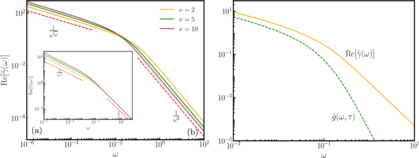
The spectral function of the reservoir, defined as the Fourier transform of the dissipation kernel , plays an important role in determining the transport properties of a system driven by the reservoir. Clearly, for the real function given in Eq. (16), we must have and . Hence, it suffices to compute the spectrum for , which is given by,
| (17) |
For small , both and decay as , consistent with the large behaviour of . On the other hand, for large , and decay as and respectively. Figure 2(a) illustrates these asymptotic behaviours of and .
Noise autocorrelation: We characterize the effective noise defined in Eq. (14) by computing its mean and auto-correlation. Since the self-propulsion force is assumed to be a stationary process with a zero mean, we must have . The autocorrelation of the effective noise can be written using Eq. (14) and Eq. (5) as,
| (18) | |||
| (19) |
The sum over can be immediately performed using the identity , which also allows us to perform the sum over . Finally, we arrive at,
| (20) |
In the thermodynamic limit , the sum over can be replaced by an integral over , which leads to,
| (21) |
where
| (22) |
For our purpose, it is convenient to write down the noise autocorrelation in the frequency domain,
| (23) |
Using Eq. (21) in Eq. (23), and performing the integrals over and , we get,
| (24) |
The integrals over and can also be performed exactly, leading to,
| (25) |
with the effective noise spectrum of the active bath given by,
| (26) |
Here denotes the spectrum of the active noise. Performing the integral over , it turns out that,
| (27) |
where is given in Eq. (17). The above equation is one of the main results of this work and represents the modified FDR for the active Rubin bath. For an equilibrium bath at temperature , consisting of passive oscillators, Eq. (27) would reduce to the usual form of FDT . The temperature being replaced by a frequency-dependent function indicates that, in general, such an active bath cannot be described by an effective temperature picture.
In what follows, we will mostly consider the case where the active oscillators follow a run-and-tumble dynamics, i.e., is a dichotomous noise that alternates between stochastically with a rate . The corresponding the autocorrelation Eq. (2) decays exponentially,
| (28) |
which in the frequency domain becomes a Lorentzian,
| (29) |
III Harmonic chain driven by active Rubin baths
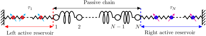
In this section, we investigate the stationary state properties of a one-dimensional extended system, modeled by a harmonic chain, driven by two active Rubin baths defined in the previous section [see Fig. 3]. We consider a chain of oscillators, each of mass , coupled with its nearest neighbors by a harmonic spring of stiffness . The left and right boundary oscillators are coupled to two active reservoirs with activities and , respectively. Let denote the displacement of the -th oscillator from its equilibrium position. In the limit of thermodynamically large reservoirs, using the results of the previous section [see Eq. (12)], the equations of motion describing the time-evolution of can be written as,
| (30) | |||||
| (31) | |||||
Note that, for simplicity, we have assumed that the dissipation kernel is the same for the two reservoirs i.e., the friction coefficient and the coupling constant are the same for both the reservoirs. However, the different activities of the reservoirs lead to different effective noises and , which are independent of each other. This activity drive leads to a NESS of the harmonic chain which we characterize in the following.
We start by solving Eq. (31), which is most conveniently done by using a matrix notation, which recasts Eq. (31) as,
| (32) |
where , is the mass matrix with elements and is the tridiagonal coupling matrix with elements,
| (33) |
The elements of the dissipation kernel matrix and the noise vector are given by,
| (34) |
Taking a Fourier transform, defined by , of Eq. (32), we get an algebraic matrix equation in the frequency domain,
| (35) |
where is the Fourier transform of . is the Greens function matrix [40, 41, 42] given by,
| (36) |
Clearly, is a tridiagonal matrix.
The displacement of the -th oscillator can be written from Eq. (36) as,
| (37) |
where the Fourier transforms of the effective noises and are given by [see Eq. (27)],
| (38) |
Our goal is to characterize the NESS of the activity-driven harmonic chain by computing the stationary kinetic temperature profile , two-time velocity autocorrelation of a single oscillator , equal time velocity-velocity correlation and the average current flowing through the system. However, before going to the activity-driven case, we present a brief overview of the thermally driven scenario which will be useful to discern the effect of activity.
III.1 Harmonic chain driven by thermal Rubin bath
The reservoir introduced in Sec. II reduces to a thermal one at temperature when the active noise in Eq. (7) is replaced by a white noise with autocorrelation . In this case, the effective noise spectrum and the dissipation kernel are related by the FDT,
| (39) |
The nonequilibrium stationary state of a harmonic chain driven by two such thermal reservoirs has been studied extensively [43, 41]. The resulting NESS is characterized by an energy current proportional to the temperature difference of the two reservoirs with temperature and respectively and a uniform kinetic temperature profile, given by the average temperature of the reservoirs, . In fact, the velocities of the bulk oscillators become uncorrelated in the thermodynamic limit i.e.,
| (40) |
Moreover, the two-time velocity correlation of a single oscillator in the bulk is given by,
| (41) |
where is the -th order Bessel function of the first kind [36]. Note that, although to the best of our knowledge, Eqs. (40) and (41) have not been reported in this form, these come out as a result of a straightforward calculation, which is discussed later in Secs. III.2.1 and III.2.3. In the following, we investigate how the activity drive affects these observables.
III.2 Stationary state correlations
We start with the velocity correlation of the bulk oscillators. In general, the two-point velocity correlation of the -th oscillator, is given by using Eq. (37) can be easily written as,
| (42) |
where we have used Eqs. (37) and (38). To compute such correlations, we need the matrix elements , which can be computed explicitly owing to the tridiagonal structure of [see Appendix B]. In particular, the relevant elements for the calculation of the correlations are given by,
| (43) |
where and are related by
| (44) |
Moreover, we have defined,
| (45) | ||||
| (46) |
for notational simplicity. We are particularly interested in the correlation among the bulk oscillators, i.e., , and in the thermodynamic limit , where the contribution to the integral Eq. (47) from frequency regime vanishes exponentially. Moreover, in this limit, one can integrate over the fast oscillations [see Appendix B for details], which yields,
| (47) |
As expected, the spatio-temporal two-point correlation in the bulk is a function of the distance between the two oscillators , and time separation . In the following, we separately discuss the equal-time spatial correlation , and the two-time correlation of a single oscillator in the bulk.
III.2.1 Velocity-velocity correlation
The velocity-velocity spatial correlation can be obtained by putting in Eq. (47),
| (48) |
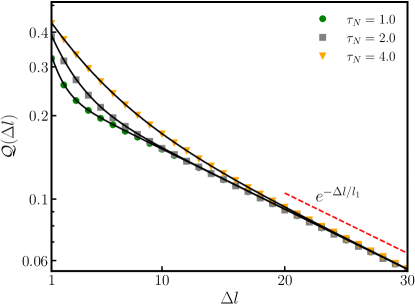
where we have used Eq. (44). For the above integral is dominated by the contributions coming from the small regime and can be approximated as,
| (49) |
where .
Clearly, the active drive leads to the emergence of two characteristic length scales associated with the reservoirs, and velocities of the bulk oscillators are correlated over a separation , determined by the reservoir with larger activity. The emergence of such a finite correlation is a direct consequence of the breaking of FDT and has been seen in the context of a boundary resetting-driven harmonic chain [44] and is also expected to appear for simpler models of active reservoirs [16, 17]. This is in sharp contrast to the thermally driven scenario, where the velocities of the bulk oscillators are uncorrelated [see Eq. (40)]. The above prediction (49) is compared with the numerical simulations in Fig. 4 which shows an excellent agreement.
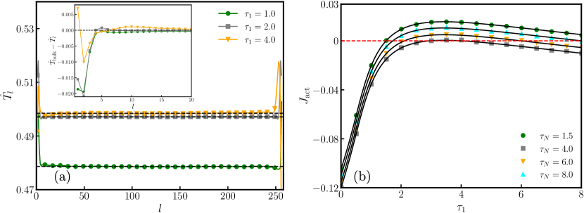
III.2.2 Kinetic temperature profile
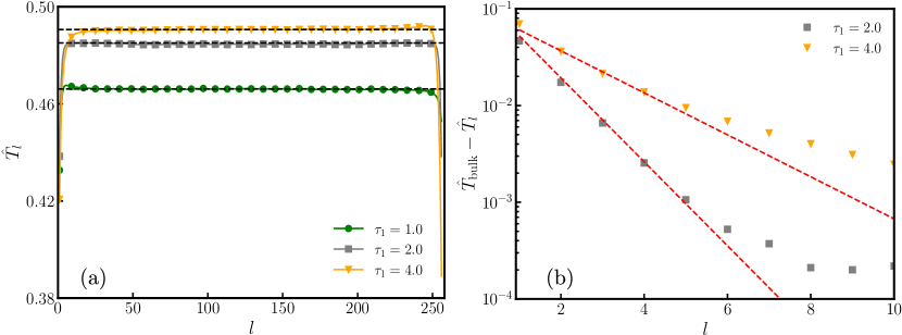
The kinetic temperature of the -th oscillator is defined as the average kinetic energy in the steady state. From Eq. (48), it is clear that, in the thermodynamic limit, the kinetic temperatures of the bulk oscillators attain a uniform value. This bulk kinetic temperature , obtained by putting in Eq. (48), is given by,
| (50) |
It is noteworthy that the bulk kinetic temperature does not depend on the dissipation kernel, and is determined only by the activity of the reservoirs. In fact, the form of is the same obtained in Ref. [16], where the active reservoir was modeled by a single correlated force. In fact, it has also been shown that, although the form of Eq. (50) is tempting [see Sec. III.1] to associate an effective temperature to the -th active reservoir, such a picture does not capture the effect of activity, except in the passive limit . In this limit, , and the bulk temperature can be expressed as,
| (51) |
III.2.3 Two-time velocity correlation
Next, we focus on the stationary two-time velocity autocorrelation of a single oscillator, which can be obtained by putting in Eq. (47). Using Eqs. (44) and (29), it is most conveniently expressed as,
| (52) |
To evaluate the -integral, we use the variable transformation , which recasts Eq. (52) as,
| (53) |
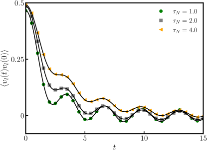
The above integral can be numerically evaluated to obtain the two-time velocity correlation at all times. Figure 6 shows the temporal decay of for different values of activity drive. The oscillatory nature of the two-time correlation is qualitatively similar to the thermally driven case [see Eq. (41)] and it is useful to investigate the effect of activity quantitatively.
To this end, we evaluate the integral in Eq. (53) term by term by expanding in a power series of , which leads to,
| (54) | ||||
| (55) |
Here denotes the regularized generalized Hypergeomatric function [36]. To understand the effect of activity on two-time velocity correlation, it is useful to analyze the asymptotic behavior of in the short-time () and long-time () regimes.
To extract the short-time behavior of we first expand for small values of [36],
| (56) |
Substituting the above equation in Eq. (55) and performing the sum over , we get,
| (57) |
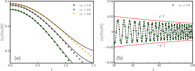
where is defined in Eq. (50). Note that, as expected, in the limit, converges to the bulk kinetic temperature [see Eq. (50)]. The short-time behavior of the two-time correlation is illustrated in Fig. 7(a). It is noteworthy that the anomalous short-time behavior Eq. (57), which is qualitatively different than the same in the thermally driven scenario [see Eq. (41)], shows strong signatures of activity.
To obtain the large-time behavior of , we note that for large ,
| (58) |
Using the above equation in Eq. (55) we get the large-time behavior of the two-time velocity correlation ,
| (59) |
where is defined in Eq. (50). The large time behavior of is shown in Fig. 7(b), which illustrates its oscillatory decay with a envelop.
It is noteworthy that Eq. (59) is similar to Eq. (41), i.e., the velocity two-time correlation in the thermally driven scenario, but with a prefactor different from the bulk kinetic temperature . This provides additional evidence that can not be thought of as an effective temperature for the active reservoirs, in general. However, as mentioned before, a consistent effective temperature picture arises in the passive limit , where Eq. (59) resembles Eq. (51) with playing the role of the effective temperature of the -th bath.
III.3 Stationary state current
The active reservoirs coupled to the boundary oscillators are expected to drive an energy current through the system when . To compute this current, it suffices to consider the instantaneous work done by one of the reservoirs (say, the left one) on the corresponding boundary oscillator. Thus, in the stationary state, the average energy current is given by [42, 40, 41],
| (60) |
This average active current can be computed using the Green’s function formalism introduced in Ref. [41] and adapted for nonequilibrium baths in Ref. [16, 17]. The details of the computation are provided in Appendix C; here we quote the main result. The active current is given by a ‘Landauer-like’ formula,
| (61) |
where the matrix , dissipation kernel and the autocorrelation of the active noise are defined in Eqs. (36), (17) and (29), respectively. Note that, the presence of frequency-dependent function in Eq. (61), which is indicative of the violation of FDR of the active reservoir, distinguishes the above expression from the case of the equilibrium bath [see Eq. (67) of Ref. [40]].
We are particularly interested in the thermodynamic limit , where Eq. (61) reduces to [see Appendix C],
| (62) |
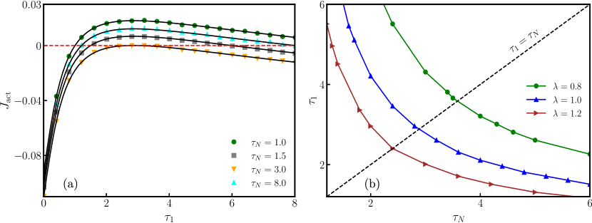
Although the integral in the above equation can not be performed exactly to obtain a closed form for , it can be evaluated numerically to arbitrary accuracy for any values of . This is illustrated in Fig. 8(a) where we have plotted the analytical prediction Eq. (62) with measured from numerical simulations which shows an excellent agreement.
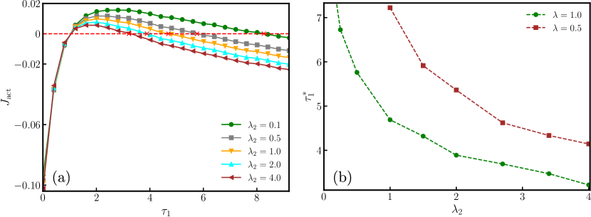
From Fig. 8(a) it is apparent that the active current shows a non-monotonic behavior as a function of as well as a non-trivial direction reversal at . This reversal point depends on reservoir coupling strength which is illustrated in Fig. 8(b) where is plotted as a function of for three different values of . As the average current is a nonmonotonic function of , the differential conductivity for a range of . The negative differential conductivity and nontrivial direction reversal are also reported in Ref. [16] using a much more simplified version of the active reservoir. The emergence of these features, even for the microscopic model of the active reservoir, indicates that these behaviors are rather robust which we illustrate in the following section using a more generalized model of the active reservoir.
IV Generalizations to non-Markovian and non-linear reservoirs
The linear nature of the active chain and the Poissonian tumbling protocol makes the active Rubin model analytically treatable. An obvious question is whether the results obtained so far are special due to the simplicity of this model. In this section, we investigate this question by generalizing the model of the active reservoir by introducing a Non-markovian tumbling protocol and non-linear interactions among the reservoir particles. It turns out that the qualitative behavior of the NESS remains the same in both of these cases, which illustrates the robustness of our results.
IV.1 Non-Markovian tumbling protocol
In general, the waiting time between two consecutive tumblings of the RTPs can be drawn from a distribution . The constant rate Markovian protocol considered so far corresponds to the case where the waiting-time distribution is exponential i.e., . One of the simplest ways to introduce a non-Markovian flipping protocol is to consider a Gamma-distribution for the waiting time, where still characterizes the activity. The corresponding autocorrelation of the active force in the time as well as in the frequency domain are given by [45, 46],
| (63) |
respectively. In this section, we discuss how the NESS of the activity-driven harmonic chain changes when the reservoir particles follow this particular flipping protocol.
The two-point velocity correlation of the bulk oscillator , in this case, can be obtained by substituting Eq. (63) and in Eq. (47). The integration can be performed exactly and yields,
| (64) |
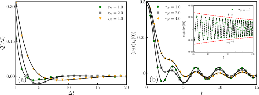
Clearly, in this case, too, we have the emergence of the two active length scales which remain the same as in the constant rate flipping case. However, the exponential decays are modulated by an oscillator function which makes it allows negative values for the correlation for some values of . Fig. 9(a) illustrates the oscillator behavior of for different values of the activity drive.
The two-time velocity correlation of a single oscillator for the non-Markovian flipping protocol can also be obtained by using Eq. (63) in Eq. (47) and substituting and . This leads to,
| (65) |
which can be evaluated numerically for all time. In the long-time limit , the dominant contribution to the integral in Eq. (65) comes from the region and one can get a closed form expression,
| (66) |
The temporal decay of for the non-Markovian tumbling protocol is shown in fig. 9(b).
It is also straightforward to calculate the bulk kinetic temperature, which, in this case, turns out to be,
| (67) |
Figure 10(a) shows the kinetic temperature profile for different values of . Interestingly, the non-Markovian flipping protocol gives rise to an oscillatory behavior in the boundary layer, which is illustrated in the inset of Figure 10(a). In the passive limit , an effective thermal picture emerges and the can be expressed as,
| (68) |
Clearly, the effective temperature of the -th reservoir, for the non-Markovian tumbling protocol, is reduced with respect to the Markovian case [see Eq. (51)].
Finally, one can calculate the stationary state current by substituting Eq. (63) in the Eq. (62) and integrating it numerically. In Fig. 10(b) we have shown the analytical prediction of with the numerical simulation. From Fig. 10(b), it is clear that the most important qualitative features of the namely the negative differential conductivity and the non-trivial sign reversal, mentioned in Sec. III.3, remain unaffected irrespective of change in the active force autocorrelation .
IV.2 Nonlinear active Rubin bath
Finally, in this section, we explore the effect of non-linear interactions in the active reservoirs. In particular, we consider the interparticle potential [see Eqs. Eq. (4) and Eq. (6)] to be of the famous Fermi-Pasta-Ulam-Tsingou form [47, 48],
| (69) |
Due to the non-linear nature of the corresponding equations of motion Eq. (4), it is difficult to obtain the effective equation of motion for the probe particle Eq. (6). We use numerical simulations to measure the stationary current flowing through the system. Fig. 11(a) shows the plot of for different values of the non-linear coupling constant . Clearly, the qualitative behavior of the current does not change—it shows a non-monotonic behavior as the activity drive is changed and undergoes a direction reversal at some non-trivial point . However, this reversal point now depends on the non-linear coupling strength— decreases monotonically as is increased. Figure 11(b) shows a plot of for different values of .
V Conclusions
In this work, we propose a model for an active Rubin bath—a microscopic model for an active reservoir in the form of a harmonic chain of overdamped run-and-tumble particles. The activity of such a reservoir is characterized by the persistence time of the constituent particles, which are assumed to be the same. We characterize the behavior of this active reservoir by explicitly computing the dissipation and noise kernels experienced by a passive inertial probe connected to it. The active nature of the reservoir leads to a modification of the FDR which can not be described by an effective temperature picture.
We also study the properties of an ordered harmonic chain driven by two such active reservoirs with different activities and . We characterize the NESS of the activity-driven system by computing the two-point correlation of the velocity of the bulk oscillators, kinetic temperature profile, and the average energy current flowing through the system. It turns out that the activity-driven NESS is characterized by several novel features compared to its thermally-driven counterpart. First, the active nature of the drive gives rise to a characteristic length scale over which the velocities of the bulk oscillators are correlated. This is in sharp contrast to the thermally-driven scenario where the velocity fluctuations of the bulk oscillators are uncorrelated. The two-time velocity correlation of a single oscillator also shows strong signatures of the activity in the short-time regime. Moreover, the average energy current shows a nonmonotonic behavior, accompanied by a nontrivial direction-reversal, as the activity drive is changed. It is to be noted that none of these behaviors, in general, can be explained by an effective temperature picture except in the passive limit . We also perform numerical simulations with more generalized models for the active reservoirs by considering FPUT-type interactions among the reservoir particles and non-Markovian activity dynamics and find the same qualitative behavior of the energy current.
The results obtained here and in some of our recent works [16, 17] suggest that the striking features of the current, namely, the non-monotonicity and the direction reversal are rather generic to the activity-driven harmonic systems. In this context, it would be interesting to investigate if other microscopic models of active reservoirs with hardcore or short-ranged interactions can lead to qualitative changes in the behavior of the energy current. Another relevant question is how the characteristic properties of the NESS change in the presence of disorder and correlated dynamics of the constituents of the reservoir particles. Finally, it is also worthwhile to investigate whether the qualitative behavior of the energy current changes in the presence of disorder and non-linearity in the driven system.
Acknowledgements.
R. S. acknowledges support from the CSIR, India [Grant No. 09/0575(11358)/2021-EMR-I]. U.B. acknowledges support from the Science and Engineering Research Board (SERB), India, under a MATRICS grant [No. MTR/2023/000392].Appendix A Derivation of the generalized Langevin equation
In this section, we provide the details of the computation of the effective noise and the dissipation kernel acting on the passive probe particle [see Fig. 1]. We start from Eq. (7), which can be conveniently recast in a matrix form,
| (70) |
where and . The information about the linear interaction of the active particles is encoded in the tridiagonal matrix with elements
| (71) |
Finally, encodes the position of the probe particle while matrix with the elements denotes the coupling between the reservoir and the probe particle.
Our goal is to write an equation of motion for the probe particle, by integrating out the reservoir particle positions . To this end, we first need to find the solution of Eq. (70) for a given , which can most conveniently be obtained by diagonalizing the tri-diagonal matrix [49]. The eigenvalues of are given by,
| (72) |
and the -th component of the normalized eigenvector corresponding to is,
| (73) |
Thus, is diagonalized by the similarity transformation,
| (74) |
where the diagonal matrix has the elements and the diagonalizing matrix with elements satisfies . Multiplying Eq. (70) with from the left, we get,
| (75) |
which can be readily integrated to obtain,
| (76) |
Using the explicit form of , and , we finally get,
| (77) |
where we have defined,
| (78) |
which is also quoted in Eq. (10) in the main text. Taking we get the equation of motion of , given in Eq. (9).
Appendix B Computation of the velocity correlation
In this appendix, we provide the details of the computation for the two-point correlation of the velocities of the bulk oscillators. Using Eq. (42), the two-point correlation can be written as a sum of the contributions coming from the reservoirs as,
| (79) |
with,
| (80) |
Here is the Greens’s function matrix defined in Eq. (36). Because of the tridiagonal nature of , the elements of can be computed explicitly [50]. The relevant elements required for our purpose are,
| (81) |
The explicit forms of for are given by [50, 51],
| (82) | ||||
| (83) | ||||
| (84) | ||||
| (85) |
where and are related by
| (86) |
For notational simplicity, we have also defined, and in Eq. (85) with,
| (87) | |||
| (88) |
Using Eqs. (81) and (85) we can write the contribution from the left active reservoir as,
| (89) | |||
| (90) |
From Eq. (86), it is clear that, in the region , becomes imaginary and the integrand in Eq. (90) vanishes exponentially as for real . Therefore, for large , non-zero contribution to the integral comes only from the region , or . It is important to note that, the imaginary term present in Eq. (90) vanishes as it turns out to be an odd function of (or ). Moreover, we are interested in the velocity correlation in the bulk, and without any loss of generality, we can take , . Thus, for large Eq. (90) reduces to,
| (91) | |||
| (92) |
which is a function of only. In the limit , one can average over the fast oscillations in [51] to get,
| (93) |
Note that, here we have used the identities,
| (94) | |||
| (95) |
Using the explicit expression of given in Eq. (88) we get,
| (96) |
The contribution from the right active reservoir can also be calculated in a similar manner. Finally, we arrive at Eq. (47) where we have used the fact that and and the explicit form of given in Eq. (27).
Appendix C Computation of the average stationary current
The average energy current in the steady state can be written as,
| (97) |
where,
| (98) |
It is convenient to recast these quantities in a matrix notation,
| (99) |
where we have defined,
| (100) | |||
| (101) | |||
| (102) |
In the following, we evaluate and separately. Using Eq. (35) in Eq. (99), we have,
| (103) |
where is the Fourier transform of defined in Eq. (102). Next, from Eq. (38), we have,
| (104) |
Substitution of (104) in Eq. (103) yields,
| (105) |
We can proceed similarly to evaluate , which leads to,
| (106) |
Thus, using Eqs. (105) and (106) in Eq. (97), the total average energy current in the stationary state can be expressed as,
| (107) |
where we have separated the terms containing and . As shown below, the above equation can be further simplified by exploiting properties of . From Eq. (36), we have,
| (108) |
Taking the complex conjugate of and subtracting it from Eq. (108), we arrive at,
| (109) |
Using Eq. (109) in Eq. (107), we can rewrite the term containing as,
| (110) |
The first term vanishes since the integrand is an odd function of . Moreover, multiplying Eq. (108) with from right, we get,
| (111) |
Substituting Eq. (111) in Eq. (110) we arrive at,
| (112) |
Once again, the first integral in the above equation vanishes as the integrand is an odd function of . Therefore, we are left with only one term that contains . Using Eq. (107) and combining the contributions from both reservoirs, we arrive at,
| (113) |
Using explicit forms of and from Eqs. (100) and (104), and taking the trace, we arrive at a ‘Landauer-like’ formula,
| (114) |
The matrix element [see Eq. (81)], where is given by Eq. (85). For thermodynamically large system size , the integrand in Eq. (114) is non-zero only within the band [see the discussion after Eq. (90)]. Furthermore, in this thermodynamic limit, one can also integrate out the fast oscillations using Eq. (95), which leads to a rather simple expression,
| (115) |
Note that, in the last step we have used Eq. (96). Substituting Eq. (115) and Eq. (27) in Eq. (114) we arrive at Eq. (62) in the main text.
References
- Kubo [1966] R. Kubo, Rep. Prog. Phys. 29, 255 (1966).
- Maes and Thomas [2013] C. Maes and S. R. Thomas, Phys. Rev. E 87, 022145 (2013).
- Maes [2014] C. Maes, J Stat Phys 154, 705 (2014).
- Maes and Steffenoni [2015] C. Maes and S. Steffenoni, Phys. Rev. E 91, 022128 (2015).
- Vandebroek and Vanderzande [2017] H. Vandebroek and C. Vanderzande, J Stat Phys 167, 14 (2017).
- Khali et al. [2023] S. S. Khali, F. Peruani, and D. Chaudhuri, (2023), 10.48550/arXiv.2305.03830.
- Wu and Libchaber [2000] X.-L. Wu and A. Libchaber, Phys. Rev. Lett. 84, 3017 (2000).
- Maggi et al. [2014] C. Maggi, M. Paoluzzi, N. Pellicciotta, A. Lepore, L. Angelani, and R. Di Leonardo, Phys. Rev. Lett. 113, 238303 (2014).
- Granek et al. [2022] O. Granek, Y. Kafri, and J. Tailleur, Phys. Rev. Lett. 129, 038001 (2022).
- Jayaram and Speck [2023] A. Jayaram and T. Speck, Euro. Phys. Lett. (2023), 10.1209/0295-5075/acdf1a.
- Guevara-Valadez et al. [2023] C. A. Guevara-Valadez, R. Marathe, and J. R. Gomez-Solano, Physica A: Stat. Mech. Appl. 609, 128342 (2023).
- Angelani et al. [2011] L. Angelani, C. Maggi, M. Bernardini, A. Rizzo, and R. Di Leonardo, Phys. Rev. Lett. 107, 138302 (2011).
- Angelani et al. [2009] L. Angelani, R. Di Leonardo, and G. Ruocco, Phys. Rev. Lett. 102, 048104 (2009).
- Kaiser et al. [2014] A. Kaiser, A. Peshkov, A. Sokolov, B. Ten Hagen, H. Löwen, and I. S. Aranson, Phys. Rev. Lett. 112, 158101 (2014).
- Dhar and Saintillan [2024] T. Dhar and D. Saintillan, (2024), 10.48550/arXiv.2402.11358.
- Santra and Basu [2022] I. Santra and U. Basu, SciPost Phys. 13, 041 (2022).
- Sarkar et al. [2023] R. Sarkar, I. Santra, and U. Basu, Phys. Rev. E 107, 014123 (2023).
- Santra [2023] I. Santra, J. Phys. Complex. 4, 015013 (2023).
- Maes [2020] C. Maes, Phys. Rev. Lett. 125, 208001 (2020).
- Paul et al. [2024] S. Paul, A. Dhar, and D. Chaudhuri, (2024), 10.48550/arXiv.2402.11358.
- Gupta and Sivak [2021] D. Gupta and D. A. Sivak, Phys. Rev. E 104, 024605 (2021).
- Singh and Kundu [2021] P. Singh and A. Kundu, J. Phys. A: Math. Theor. 54, 305001 (2021).
- Prakash et al. [2024] S. Prakash, U. Basu, and S. Sabhapandit, (2024), 10.48550/arXiv.2402.11964.
- Malakar et al. [2018] K. Malakar, V. Jemseena, A. Kundu, K. V. Kumar, S. Sabhapandit, S. N. Majumdar, S. Redner, and A. Dhar, J. Stat. Mech. , 043215 (2018).
- Santra et al. [2020] I. Santra, U. Basu, and S. Sabhapandit, Phys. Rev. E 101, 062120 (2020).
- Fodor et al. [2016] E. Fodor, C. Nardini, M. E. Cates, J. Tailleur, P. Visco, and F. van Wijland, Phys. Rev. Lett. 117, 038103 (2016).
- Martin et al. [2021] D. Martin, J. O’Byrne, M. E. Cates, E. Fodor, C. Nardini, J. Tailleur, and F. van Wijland, Phys. Rev. E 103, 032607 (2021).
- Étienne Fodor and Cristina Marchetti [2018] Étienne Fodor and M. Cristina Marchetti, Physica A: Stat. Mech. Appl. 504, 106 (2018).
- Basu et al. [2018] U. Basu, S. N. Majumdar, A. Rosso, and G. Schehr, Phys. Rev. E 98, 062121 (2018).
- Bhadra and Banerjee [2016] C. Bhadra and D. Banerjee, J. Stat. Mech. , 043404 (2016).
- Krüger and Maes [2016] M. Krüger and C. Maes, J. Phys.: Condens. Matter 29, 064004 (2016).
- Feynman and Vernon [1963] R. Feynman and F. Vernon, Ann. Physics 24, 118 (1963).
- Rubin [1961] R. J. Rubin, J. Math. Phys. 2, 373 (1961).
- Das et al. [2020] A. Das, A. Dhar, I. Santra, U. Satpathi, and S. Sinha, Phys. Rev. E 102, 062130 (2020).
- Das and Dhar [2012] S. G. Das and A. Dhar, Eur. Phys. J. B 85, 1 (2012).
- [36] DLMF, “NIST Digital Library of Mathematical Functions,” https://dlmf.nist.gov/, Release 1.2.0 of 2024-03-15, f. W. J. Olver, A. B. Olde Daalhuis, D. W. Lozier, B. I. Schneider, R. F. Boisvert, C. W. Clark, B. R. Miller, B. V. Saunders, H. S. Cohl, and M. A. McClain, eds.
- Lizana et al. [2010] L. Lizana, T. Ambjörnsson, A. Taloni, E. Barkai, and M. A. Lomholt, Phys. Rev. E 81, 051118 (2010).
- Saito and Sakaue [2015] T. Saito and T. Sakaue, Phys. Rev. E 92, 012601 (2015).
- Panja [2010] D. Panja, J. Stat. Mech. , L02001 (2010).
- Dhar [2008] A. Dhar, Adv. Phys. 57, 457 (2008).
- Dhar [2001] A. Dhar, Phys. Rev. Lett. 86, 5882 (2001).
- Lepri [2016] S. Lepri, ed., Thermal transport in low dimensions. From statistical physics to nanoscale heat transfer (Springer Cham, 2016).
- Rieder et al. [2004] Z. Rieder, J. L. Lebowitz, and E. Lieb, J. Math. Phys. 8, 1073 (2004).
- Sarkar and Roy [2023] R. Sarkar and P. Roy, J. Stat. Mech. , 103204 (2023).
- Nava et al. [2020] L. G. Nava, R. Großmann, M. Hintsche, C. Beta, and F. Peruani, Euro. Phys. Lett. 130, 68002 (2020).
- Odde and Buettner [1998] D. J. Odde and H. M. Buettner, Biophys. J. 75, 1189 (1998).
- Fermi et al. [1955] E. Fermi, P. Pasta, S. Ulam, and M. Tsingou, Studies of the nonlinear problems, Tech. Rep. (Los Alamos National Lab.(LANL), Los Alamos, NM (United States), 1955).
- Das et al. [2014] S. G. Das, A. Dhar, and O. Narayan, J Stat Phys 154, 204 (2014).
- Kouachi [2006] S. Kouachi, ELA 15, 115 (2006).
- Usmani [1994] R. Usmani, Comput. Math. Appl. 27, 59 (1994).
- Kannan et al. [2012] V. Kannan, A. Dhar, and J. L. Lebowitz, Phys. Rev. E 85, 041118 (2012).