Sparse Extended Mean-Variance-CVaR Portfolios with Short-selling

Ahmad Mousavi Emails: {mousavi and boukouva}@american.edu, salahim@guilan.ac.ir, Maziar Salahi Department of Applied Mathematics, Faculty of Mathematical Sciences, University of Guilan Zois Boukouvalas
Abstract

This paper introduces a novel penalty decomposition algorithm customized for addressing the non-differentiable and nonconvex problem of extended mean-variance-CVaR portfolio optimization with short-selling and cardinality constraints. The proposed algorithm solves a sequence of penalty subproblems using a block coordinate descent (BCD) method while striving to fully exploit each component of the objective function or constraints. Through rigorous analysis, the well-posed nature of each subproblem of the BCD method is established, and closed-form solutions are derived where possible. A comprehensive theoretical convergence analysis is provided to confirm the efficacy of the introduced algorithm in reaching a local minimizer of this intractable optimization problem in finance, whereas generic optimization techniques either only capture a partial minimum or are not efficient. Numerical experiments conducted on real-world datasets validate the practical applicability, effectiveness, and robustness of the introduced algorithm across various criteria. Notably, the existence of closed-form solutions within the BCD subproblems prominently underscores the efficiency of our algorithm when compared to state-of-the-art methods.

1 Introduction

The mean-variance CVaR problem is crucial in finance as it provides a robust framework for optimizing portfolios by considering both expected returns (mean) and associated risks (variance and conditional value at risk). This approach helps investors balance the trade-off between maximizing returns and minimizing losses, enhancing portfolio performance and risk management in volatile markets [12, 18, 23] . Including short-selling is essential as it allows investors to profit from downward market movements, improving portfolio diversification and risk management by providing additional opportunities for profit generation in declining markets [6, 19, 24].

Moreover, sparse optimization plays a critical role in various fields such as machine learning, signal processing, and finance, offering efficient solutions for problems where the underlying data or parameters exhibit sparsity [3, 10, 13, 16, 21, 25, 26]. In portfolio optimization, having only a few assets can significantly impact diversification, potentially increasing exposure to individual asset risk and volatility, thus highlighting the importance of careful asset selection and risk management strategies. As such the cardinality constraints have been imposed in portfolio optimization models [2, 9, 14, 15, 17].

In this paper, we tackle the following extended mean-variance-CVaR portfolio problem that includes short-selling and nonconvex cardinality constraints:

$\displaystyle\min_{x\in\mathbb{R}^{n},\gamma\in\mathbb{R}}$ $\displaystyle\ f(x):=\lambda_{1}x^{T}Ax-\lambda_{2}(\Psi^{T}x-\delta\|x-\phi\|_{1})+\lambda_{3}(\gamma+\frac{1}{m(1-\beta)}\sum_{j=1}^{m}(-d_{j}^{T}x-\gamma)^{+})$ ($P$)
subject to $\displaystyle\textbf{e}^{T}x=1,\quad L\leq x\leq U,\quad\left\{\begin{array}[]{ll}x_{i}\geq 0;\,\forall i\in\Gamma^{+}:=\{i\in[n]|\,\eta_{i}>0\},\\ x_{i}\leq 0;\,\forall i\in\Gamma^{-}:=\{i\in[n]|\,\eta_{i}<0\},\\ x_{i}\in\mathbb{R};\,\forall i\in\Gamma^{0}:=\{i\in[n]|\,\eta_{i}=0\},\\ \end{array}\right.\quad\text{and}\quad\|x\|_{0}\leq k,$

where $\lambda_{1},\lambda_{2},\lambda_{3}=1-\lambda_{1}-\lambda_{2},\beta\in(0,1),\delta\geq 0,\eta,L,U\in\mathbb{R}^{n}$ with $L<U$ element-wise, $d_{j}\in\mathbb{R}^{n}$ for each $j\in[m],A\succeq 0,k\in[n]$. Also, we have

$\displaystyle\Psi=\mu+r_{c}h,\quad\eta=\mu,\quad\mbox{and}\quad d_{j}:=b_{j}-r_{c}h;\ \forall j\in[m],$

where $r_{c}\geq 0$ is the risk-neutral interest rate, $\phi_{i}$ is the proportions of the weight invested in $i$th stock and $\mu$ is the return vector. Problem ($P$) has been the subject of several research [7, 22, 20]. When $\lambda_{1}=0$, it reduces to the widely studied mean-CVaR with cardinality constraint, see for example [4, 8] and references therein.

Most recently, the authors in [7] applied the penalty decomposition method (PDM) to solve ($P$) and reported promising numerical results. Nevertheless, the full structure of the problem was not exploited. Therefore, we here introduce a novel penalty decomposition algorithm customized to fully leverage every component of the objective function in ($P$) along with its constraints. We go through a sequence of penalty subproblems that a saddle point of them is efficiently identified using a BCD method. We meticulously examine each corresponding subproblem within this BCD method to derive closed-form solutions whenever feasible. Specifically, to handle the $\|.\|_{1}$ norm in the objective function along with bound constraints, we introduce a new variable. Additionally, another variable is required to manage the softmax function in the objective function. Lastly, we resort to a third variable to address the cardinality constraint along with the short-selling constraints. Our discussions show how these new variables lead to structured subproblems and efficient We rigorously establish the convergence of our introduced algorithm towards a local minimizer of the non-differentiable problem ($P$) with non-convex constraints.

Section 2 introduces Algorithm 2, a penalty decomposition algorithm designed to tackle the non-differentiable and nonconvex problem ($P$). This algorithm employs a block coordinate Algorithm 1 to address each penalty subproblem. We establish the well-posedness of these subproblems and derive closed-form solutions for three of them. The convergence analysis of both Algorithm 1 and Algorithm 2 is provided in Section 3, demonstrating that our introduced algorithm effectively reaches a local minimizer of ($P$). Additionally, Section 4 presents extensive numerical results obtained from real-world data.

Notation. The complement of a set $S$ is denoted as $S^{c}$. We use $|S|$ to represent its cardinality. For a natural number $n$, we define $[n]$ as the set $\{1,2,\dots,n\}$. Now, consider a set $S$ given by $S=\{i_{1},i_{2},\dots,i_{|S|}\}$, which is a subset of $[n]$. For any vector $x$ in $\mathbb{R}^{n}$, we denote the coordinate projection of $x$ with respect to the indices in $S$ as $[x_{S};0]$, which means that the $i$th element of this vector equals to $x_{i}$ when $i$ belongs to $S$, and it equals to 00 for $i$ in $S^{c}$. We determine whether a matrix $A$ is positive semidefinite or definite by the notations $A\succeq 0$ and $A\succ 0$, respectively. In this paper, we let ${\rm sgn}(a):=1$ for $a>0,{\rm sgn}(a):=-1$ for $a<0,$ and ${\rm sgn}(0):=0$. For $x$ and $y\in\mathbb{R}^{n}$, $x\circ y$ shows the Hadamard (element-wise) multiplication of $x$ and $y$. Recall that

$$\partial(\|\cdot\|_{1})|_{x}\,=\,J_{1}\times J_{2}\times\cdots\times J_{n},\quad\mbox{with}\quad J_{k}=\left\{\begin{array}[]{ll}[-1,1]&\mbox{if}\quad x_{i}=0,\\ \{{\rm sgn}(x)\}&\mbox{if}\quad x_{i}\neq 0.\\ \end{array}\right.$$

and

$$\partial(\cdot)^{+}|_{x}\,=\,J_{1}\times J_{2}\times\cdots\times J_{n},\quad\mbox{with}\quad J_{k}=\left\{\begin{array}[]{ll}[0,1]&\mbox{if}\quad x_{i}=0,\\ \{1\}&\mbox{if}\quad x_{i}>0,\\ \{0\}&\mbox{if}\quad x_{i}<0.\\ \end{array}\right.$$

2 An Efficient Customized Penalty Decomposition Algorithm

Here, we propose our customized penalty decomposition algorithm for solving ($P$) that fully exploits all the available structures of the objective function and constraints of this problem.

2.1 Methodology

In this subsection, we elaborate on how we design our customized penalty decomposition algorithm. Observe that can equivalently reformulate this nonconvex problem as follows:

$\displaystyle\min_{x,y,z,w\in\mathbb{R}^{n},\gamma\in\mathbb{R}}$ $\displaystyle\ \lambda_{1}x^{T}Ax-\lambda_{2}\Psi^{T}x+\lambda_{2}\delta\|z-\phi\|_{1}+\lambda_{3}(\gamma+\frac{1}{m(1-\beta)}\sum_{j=1}^{m}(-d_{j}^{T}w-\gamma)^{+})$ (1)
subject to $\displaystyle\textbf{e}^{T}x=1,\quad y_{i}\geq 0;\,\forall i\in\Gamma^{+},\quad y_{i}\leq 0;\,\forall i\in\Gamma^{-},\quad\|y\|_{0}\leq k,\quad L\leq z\leq U,$
$\displaystyle x-y=0,\quad x-z=0,\quad\text{and}\quad x-w=0.$

Specifically, we introduce $y$ to deal with sparsity, $z$ to handle $\|.\|_{1}$, and $w$ to effectively manage the last term of the objective function in ($P$). The constraints are also accordingly decoupled using these new variables such that we possibly can obtain closed-form solutions or if not, much simpler penalty subproblems in our customized penalty decomposition algorithm (see Subsection 2.2).

More precisely, suppose that

$\displaystyle q_{\rho}(x,y,z,w,\gamma):=$ $\displaystyle\,\lambda_{1}x^{T}Ax-\lambda_{2}\Psi^{T}x+\lambda_{2}\delta\|z-\phi\|_{1}+\lambda_{3}(\gamma+\frac{1}{m(1-\beta)}\sum_{j=1}^{m}(-d_{j}^{T}w-\gamma)^{+})$
$\displaystyle+\rho(\|x-y\|_{2}^{2}+\|x-z\|_{2}^{2}+\|x-w\|_{2}^{2}),$ (2)

and

$\displaystyle\mathcal{X}:=$ $\displaystyle\,\{x\in\mathbb{R}^{n}\,|\,\textbf{e}^{T}x=1\},$
$\displaystyle\mathcal{Y}:=$ $\displaystyle\,\{y\in\mathbb{R}^{n}\,|\,y_{i}\geq 0;\,\forall i\in\Gamma^{+},\quad y_{i}\leq 0;\,\forall i\in\Gamma^{-},\quad\text{and}\quad\|y\|_{0}\leq k\}$
$\displaystyle\mathcal{Z}:=$ $\displaystyle\,\{z\in\mathbb{R}^{n}\,|\,L\leq z\leq U\}$
$\displaystyle\mathcal{W}:=$ $\displaystyle\,\{w\in\mathbb{R}^{n}\,|\,\textbf{e}^{T}w=1\quad\text{and}\quad L\leq w\leq U\}.$

In our method, we consider a sequence of penalty subproblems as follows:

$$\min_{x,y,z,w,\gamma}\quad q_{\rho}(x,y,z,w,\gamma)\qquad\textrm{subject to}\qquad x\in\mathcal{X},\quad y\in\mathcal{Y},\quad z\in\mathcal{Z},\quad w\in\mathcal{W},\quad\text{and}\quad\gamma\in\mathbb{R}$$ ($P_{x,y,z,w,\gamma}$)

The idea is that by gradually increasing the value of $\rho$ towards infinity, we can effectively address the optimization problem (1). It is important to emphasize that ($P_{x,y,z,w,\gamma}$) is yet nonconvex. However, the following BCD method efficiently converges to a saddle point of it (see Theorem 3.1).

Algorithm 1 BCD Method for Solving ($P_{x,y,z,w,\gamma}$)
1:  Input: Select arbitrary $y_{0}\in\mathcal{Y},z_{0}\in\mathcal{Z},$ and $(w_{0},\gamma_{0})\in\mathcal{W}\times\mathbb{R}$.
2:  Set $l=0$.
3:  $x_{l+1}=\mbox{Argmin}_{x\in\mathcal{X}}\ q_{\rho}(x,y_{l},z_{l},w_{l},\gamma_{l})$.
4:  $y_{l+1}\in\mbox{Argmin}_{y\in\mathcal{Y}}\ q_{\rho}(x_{l+1},y,z_{l},w_{l},\gamma_{l}).$
5:  $z_{l+1}=\mbox{Argmin}_{z\in\mathcal{Z}}\ q_{\rho}(x_{l+1},y_{l+1},z,w_{l},\gamma_{l}).$
6:  $(w_{l+1},\gamma_{l+1})\in\mbox{Argmin}_{(w,\gamma)\in\mathcal{W}\times\mathbb{R}}\ q_{\rho}(x_{l+1},y_{l+1},z_{l+1},w,\gamma).$
7:  $l\leftarrow l+1$ and go to step (3).

We are now prepared to introduce our penalty decomposition algorithm, which begins with a positive penalty parameter and gradually increases it until convergence is achieved. Algorithm 1 handles the corresponding subproblem for a fixed $\rho$. For the problem ($P$), we assume having a feasible point denoted as $x^{\text{feas}}$ in hand, which is easy to obtain. To present this algorithm and its subsequent analysis, we define:

$$\Upsilon\geq\max\{f(x^{\text{feas}}),\min_{x\in\mathcal{X}}q_{\rho^{(0)}}(x,y^{(0)}_{0},z^{(0)}_{0},w^{(0)}_{0},\gamma^{(0)}_{0})\}>0\qquad\text{and}\qquad X_{\Upsilon}:=\{x\in\mathbb{R}^{n}\,|\,f(x)\leq\Upsilon\}.$$ (3)
Algorithm 2 A Customized Penalty Decomposition Algorithm for Solving ($P$)
1:  Inputs: $r>1,\rho^{(0)}>0$, and $y^{(0)}_{0}\in\mathcal{Y},z^{(0)}_{0}\in\mathcal{Z},w^{(0)}_{0}\in\mathcal{W},$ and $\gamma^{(0)}_{0}\in\mathbb{R}$
2:  Set $j=0$.
3:  repeat
4:     Set $l=0$.
5:     repeat
6:        Solve $x^{(j)}_{l+1}\in\mbox{Argmin}_{x\in\mathcal{X}}\ q_{\rho}(x,y^{(j)}_{l},z^{(j)}_{l},w^{(j)}_{l},\gamma^{(j)}_{l})$ [see (8)].
7:        Solve $y^{(j)}_{l+1}=\mbox{Argmin}_{y\in\mathcal{Y}}\ q_{\rho}(x^{(j)}_{l+1},y,z^{(j)}_{l},w^{(j)}_{l},\gamma^{(j)}_{l})$ [see (9)].
8:        Solve $z^{(j)}_{l+1}=\mbox{Argmin}_{z\in\mathcal{Z}}\ q_{\rho}(x^{(j)}_{l+1},y^{(j)}_{l+1},z,w^{(j)}_{l},\gamma^{(j)}_{l})$ [see (11)].
9:        Solve $(w^{(j)}_{l+1},\gamma^{(j)}_{l+1})\in\mbox{Argmin}_{(w,\gamma)\in\mathcal{W}\times\mathbb{R}}\ q_{\rho}(x^{(j)}_{l+1},y^{(j)}_{l+1},z^{(j)}_{l+1},w,\gamma)$ [see (16)].
10:        Set $l\leftarrow l+1$.
11:     until stopping criterion (4) is met.
12:     Set $\rho^{(j+1)}=r\cdot\rho^{(j)}$.
13:     Set $(x^{(j)},y^{(j)},z^{(j)},w^{(j)},\gamma^{(j)}):=(x^{(j)}_{l},y^{(j)}_{l},z^{(j)}_{l},w^{(j)}_{l},\gamma^{(j)}_{l})$.
14:     If $\min_{x\in\mathcal{X}}q_{\rho^{(j+1)}}(x,y^{(j)},z^{(j)},w^{(j)},\gamma^{(j)})>\Upsilon$, then $y_{0}^{(j+1)}=z_{0}^{(j+1)}=w_{0}^{(j+1)}=x^{\text{feas}}$ and $\gamma^{(j+1)}_{0}=\gamma^{\text{feas}}$. Otherwise, $y^{(j+1)}_{0}=y^{(j)},z^{(j+1)}_{0}=z^{(j)},w^{(j+1)}_{0}=w^{(j)}$, and $\gamma^{(j+1)}_{0}=\gamma^{(j)}$.
15:     Set $j\leftarrow j+1$.
16:  until stopping criterion (5) is met.

We stop the inner loop if

$$\max\left\{\frac{\|x_{l}-x_{l-1}\|_{\infty}}{\max\left(\|x_{l}\|_{\infty},1\right)},\frac{\|y_{l}-y_{l-1}\|_{\infty}}{\max\left(\|y_{l}\|_{\infty},1\right)},\frac{\|z_{l}-z_{l-1}\|_{\infty}}{\max\left(\|z_{l}\|_{\infty},1\right)},\frac{\|w_{l}-w_{l-1}\|_{\infty}}{\max\left(\|w_{l}\|_{\infty},1\right)},\frac{|\gamma_{l}-\gamma_{l-1}|}{\max\left(|\gamma_{l}|,1\right)}\right\}\leq\epsilon_{I},$$ (4)

and the outer loop when a convergence criterion is met:

$$\|x^{(j)}-y^{(j)}\|_{\infty}+\|x^{(j)}-z^{(j)}\|_{\infty}+\|x^{(j)}-w^{(j)}\|_{\infty}\leq\epsilon_{O}.$$ (5)

2.2 Subproblems of Algorithm 1

We discuss how to efficiently solve the constrained subproblems presented in Algorithm 1 below.

2.2.1 Subproblem of $x$

This subproblem ($\min_{x\in\mathcal{X}}\ q_{\rho}(x,y,z,w,\gamma)$) becomes the following convex quadratic optimization problem:

$\displaystyle\min_{x\in\mathbb{R}^{n}}$ $\displaystyle\lambda_{1}x^{T}Ax-\lambda_{2}\Psi^{T}x+\rho(\|x-y\|_{2}^{2}+\|x-z\|_{2}^{2}+\|x-w\|_{2}^{2})\qquad\textrm{subject to}\qquad\textbf{e}^{T}x=1.$ ($P_{x}$)

Since $A\succeq 0$ and $\rho>0$, we have $A+3\rho I\succ 0$. Hence, this strictly convex problem has a unique solution, and, for $t\in\mathbb{R}$, its KKT conditions are as follows:

$$2\lambda_{1}Ax_{*}-\lambda_{2}\Psi+2\rho(3x_{*}-y-z-w)+t\textbf{e}=0,\quad\mbox{and}\quad\textbf{e}^{T}x_{*}=1.$$ (6)

Thus, $2(\lambda_{1}A+3\rho I)x_{*}=2\rho(y+z+w)+\lambda_{2}\Psi-t\textbf{e}$. By letting

$$B:=\lambda_{1}A+3\rho I\qquad\text{and}\qquad\vartheta:=2\rho(y+z+w)+\lambda_{2}\Psi,$$ (7)

we see $x_{*}=0.5B^{-1}(\vartheta-t\textbf{e})$, which together with $1=\textbf{e}^{T}x_{*}=0.5\textbf{e}^{T}B^{-1}(\vartheta-t\textbf{e})$ implies

$$t=\frac{-1+0.5\textbf{e}^{T}B^{-1}\vartheta}{0.5\textbf{e}^{T}B^{-1}\textbf{e}},$$

This in turn yields

$$x_{*}=\frac{1}{2}B^{-1}\left(\vartheta+\frac{1-0.5\textbf{e}^{T}B^{-1}\vartheta}{0.5\textbf{e}^{T}B^{-1}\textbf{e}}\textbf{e}\right).$$ (8)

2.2.2 Subproblem of $y$

Recall that we let ${\rm sgn}(0)=0,$ so by slightly abusing the notation, this subproblem ($\min_{y\in\mathcal{Y}}\ q_{\rho}(x,y,z,w,\gamma)$) is as follows:

$$\min_{y\in\mathbb{R}^{n}}\ \|x-y\|_{2}^{2}\qquad\mbox{subject to}\qquad{\rm sgn}(\eta)\circ y\geq 0,\quad\textrm{and}\quad\|y\|_{0}\leq k.$$ ($P_{y}$)

To provide a closed-form solution to the latter problem, we first define the following generalized sparsifying operator.

Definition 2.1.

Let $x$ and $\mu\in\mathbb{R}^{n}$ and a natural number $k\in[n]$ be given. Denote $x^{+}=\max(x,0),\,x^{-}=\max(-x,0),\,\Gamma^{+}=\{i\,|\,\eta_{i}>0\},\,\Gamma^{-}=\{i\,|\,\eta_{i}<0\},$ and $\Gamma^{0}=[n]-(\Gamma^{+}\cup\Gamma^{-})=\{i\,|\,\eta_{i}=0\}$. Then, the generalized sparsifying operator $\mathcal{S}_{k,\eta}(x)$ is defined as follows:

$$\mathcal{S}_{k,\eta}(x)=([x^{+}_{\Gamma^{+}};0]-[x^{-}_{\Gamma^{-}};0]+[x_{\Gamma^{0}};0])_{\mathcal{J}}$$ (9)

where $\mathcal{J}$ is an index set corresponding to the $k$ largest components of $[x^{+}_{\Gamma^{+}};0]-[x^{-}_{\Gamma^{-}};0]+[x_{\Gamma^{0}};0]$ in absolute value.

Lemma 2.1.

The solution to the problem ($P_{y}$) is $y_{*}=\mathcal{S}_{k,\eta}(x)$ defined in (9).

Proof.

For any $y$ with $\|y\|_{0}\leq k$, we can write $y=[y_{\mathcal{I}};y_{\mathcal{I}^{c}}]$ such that $y_{\mathcal{I}}=0$ for some index set $\mathcal{I}\subseteq[n]$ with $|\mathcal{I}|=n-k$. Hence, for any index set $\mathcal{I}$ with $|\mathcal{I}|=n-k$, $(P_{y})$ can be written as the following indexed problem:

$$\min_{y\in\mathbb{R}^{n}}(\|x_{\mathcal{I}}-y_{\mathcal{I}}\|^{2}_{2}+\|x_{\mathcal{I}^{c}}-y_{\mathcal{I}^{c}}\|^{2}_{2})\qquad\text{subject to}\qquad{\rm sgn}(\eta_{i})y_{i}\geq 0;\quad\forall i,\quad\text{and}\quad y_{\mathcal{I}}=0,$$

which is equivalent to solving:

$$\min_{\theta\in\mathbb{R}^{|\mathcal{I}^{c}|}}\|\theta-x_{\mathcal{I}^{c}}\|^{2}_{2}\qquad\,\ \text{subject to}\,\qquad{\rm sgn}(\eta_{i})\theta_{i}\geq 0;\quad\forall i\in\mathcal{I}^{c}.$$

For any $i\in\Gamma^{0}\cap\mathcal{I}^{c}$, we do not have any constraints, which shows that $(\theta_{*})_{i}=x_{i}$ for all $i\in\Gamma^{0}\cap\mathcal{I}^{c}$. Thus, by letting $\Gamma=\mbox{supp}(\mu)=\Gamma^{+}\cup\Gamma^{-}$, it suffices to only focus on the following:

$$\min_{\nu\in\mathbb{R}^{|\Gamma\cap\mathcal{I}^{c}|}}\|\nu-x_{\Gamma\cap\mathcal{I}^{c}}\|^{2}_{2}\qquad\,\ \text{subject to}\,\qquad{\rm sgn}(\eta_{i})\nu_{i}\geq 0;\quad\forall i\in\Gamma\cap\mathcal{I}^{c}.$$

The KKT conditions for the global minimizer $\nu_{*}$ of this strictly convex problem can be written as:

$$x_{\Gamma\cap\mathcal{I}^{c}}=\nu_{*}-\zeta\circ({\rm sgn}(\eta))_{\Gamma\cap\mathcal{I}^{c}}\quad\text{and}\quad\nu_{*}\circ({\rm sgn}(\eta))_{\Gamma\cap\mathcal{I}^{c}}\geq 0,\quad\text{with}\quad\zeta\geq 0\quad\text{and}\quad\zeta^{T}({\rm sgn}(\eta)\circ\nu_{*})=0.$$

Let $a=({\rm sgn}(\eta)\circ x)_{\Gamma\cap\mathcal{I}^{c}}$, then it is known that $a=a^{+}-a^{-}$ for $a^{+}=\max(a,0)$ and $a^{-}=\max(-a,0)$ and $a^{+}\perp a^{-}$. It is easy to see that $(\nu_{*})_{i}={a_{i}^{+}}/{{\rm sgn}(\eta_{i})}$ and $\zeta_{i}={a^{-}_{i}}$ for any $i\in\Gamma\cap\mathcal{I}^{c}$, that is,

$$\nu_{*}={\rm sgn}(\eta)\circ({\rm sgn}(\eta)\circ x)^{+}_{\Gamma\cap\mathcal{I}^{c}}\qquad\text{and}\qquad\zeta=({\rm sgn}(\eta)\circ x)^{-}_{\Gamma\cap\mathcal{I}^{c}}$$

satisfy the given KKT conditions above. By recalling $\Gamma^{+}$ and $\Gamma^{-}$ defined inside ($P$), we see

$$(\nu_{*})_{\Gamma^{+}\cap\mathcal{I}^{c}}=x^{+}_{\Gamma^{+}\cap\mathcal{I}^{c}}\qquad\text{and}\qquad(\nu_{*})_{\Gamma^{-}\cap\mathcal{I}^{c}}=-x^{-}_{\Gamma^{-}\cap\mathcal{I}^{c}}.$$

Therefore, we have

$$(\theta_{*})_{\Gamma^{0}\cap\mathcal{I}^{c}}=x_{\Gamma^{0}\cap\mathcal{I}^{c}},\qquad(\theta_{*})_{\Gamma^{+}\cap\mathcal{I}^{c}}=x^{+}_{\Gamma^{+}\cap\mathcal{I}^{c}},\qquad\text{and}\qquad(\theta_{*})_{\Gamma^{-}\cap\mathcal{I}^{c}}=-x^{-}_{\Gamma^{-}\cap\mathcal{I}^{c}}.$$

So, for any index $\mathcal{I}$ specified above, the optimal value of the indexed problem is given by

$\displaystyle\|x_{\mathcal{I}^{c}}-\theta_{*}\|^{2}_{2}+\|x_{\mathcal{I}}\|^{2}_{2}$ $\displaystyle=$ $\displaystyle\|x_{\Gamma^{+}\cap\mathcal{I}^{c}}-x^{+}_{\Gamma^{+}\cap\mathcal{I}^{c}}\|^{2}_{2}+\|x_{\Gamma^{+}\cap\mathcal{I}}\|^{2}_{2}$
$\displaystyle+$ $\displaystyle\|x_{\Gamma^{-}\cap\mathcal{I}^{c}}+x^{-}_{\Gamma^{-}\cap\mathcal{I}^{c}}\|^{2}_{2}+\|x_{\Gamma^{-}\cap\mathcal{I}}\|^{2}_{2}$
$\displaystyle+$ $\displaystyle\|x_{\Gamma^{0}\cap\mathcal{I}^{c}}-x_{\Gamma^{0}\cap\mathcal{I}^{c}}\|^{2}_{2}+\|x_{\Gamma^{0}\cap\mathcal{I}}\|^{2}_{2},$

where

$$\|x_{\Gamma^{+}\cap\mathcal{I}^{c}}-x^{+}_{\Gamma^{+}\cap\mathcal{I}^{c}}\|^{2}_{2}+\|x_{\Gamma^{+}\cap\mathcal{I}}\|_{2}^{2}=\|x_{\Gamma^{+}\cap\mathcal{I}^{c}}\|_{2}^{2}-\|x^{+}_{\Gamma^{+}\cap\mathcal{I}^{c}}\|^{2}_{2}+\|x_{\Gamma^{+}\cap\mathcal{I}}\|_{2}^{2}=\|x_{\Gamma^{+}}\|^{2}_{2}-\|x^{+}_{\Gamma^{+}\cap\mathcal{I}^{c}}\|_{2}^{2},$$
$$\|x_{\Gamma^{-}\cap\mathcal{I}^{c}}+x^{-}_{\Gamma^{-}\cap\mathcal{I}^{c}}\|^{2}_{2}+\|x_{\Gamma^{-}\cap\mathcal{I}}\|_{2}^{2}=\|x_{\Gamma^{-}\cap\mathcal{I}^{c}}\|_{2}^{2}-\|x^{-}_{\Gamma^{-}\cap\mathcal{I}^{c}}\|^{2}_{2}+\|x_{\Gamma^{-}\cap\mathcal{I}}\|_{2}^{2}=\|x_{\Gamma^{-}}\|^{2}_{2}-\|x^{-}_{\Gamma^{-}\cap\mathcal{I}^{c}}\|_{2}^{2},$$

and

$$\|x_{\Gamma^{0}\cap\mathcal{I}^{c}}-x_{\Gamma^{0}\cap\mathcal{I}^{c}}\|^{2}_{2}+\|x_{\Gamma^{0}\cap\mathcal{I}}\|_{2}^{2}=\|x_{\Gamma^{0}}\|^{2}_{2}-\|x_{\Gamma^{0}\cap\mathcal{I}^{c}}\|_{2}^{2}.$$

Consequently, the optimal value becomes

$\displaystyle\|x_{\mathcal{I}^{c}}-\theta_{*}\|^{2}_{2}+\|x_{\mathcal{I}}\|^{2}_{2}$ $\displaystyle=$ $\displaystyle\|x_{\Gamma^{+}}\|^{2}_{2}-\|x^{+}_{\Gamma^{+}\cap\mathcal{I}^{c}}\|_{2}^{2}$
$\displaystyle+$ $\displaystyle\|x_{\Gamma^{-}}\|^{2}_{2}-\|x^{-}_{\Gamma^{-}\cap\mathcal{I}^{c}}\|_{2}^{2}$
$\displaystyle+$ $\displaystyle\|x_{\Gamma^{0}}\|^{2}_{2}-\|x_{\Gamma^{0}\cap\mathcal{I}^{c}}\|_{2}^{2}$
$\displaystyle=$ $\displaystyle\|x\|^{2}_{2}-\|x^{+}_{\Gamma^{+}\cap\mathcal{I}^{c}}\|_{2}^{2}-\|x^{-}_{\Gamma^{-}\cap\mathcal{I}^{c}}\|_{2}^{2}-\|x_{\Gamma^{0}\cap\mathcal{I}^{c}}\|_{2}^{2}.$

This implies that the minimal value of (Py)Py(\ref{pr: py}) is achieved when $\|x^{+}_{\Gamma^{+}\cap\mathcal{I}^{c}}\|_{2}^{2}+\|x^{-}_{\Gamma^{-}\cap\mathcal{I}^{c}}\|_{2}^{2}+\|x_{\Gamma^{0}\cap\mathcal{I}^{c}}\|_{2}^{2}$ is maximal or equivalently when $\mathcal{I}^{c}=\mathcal{J}([x^{+}_{\Gamma^{+}};0]-[x^{-}_{\Gamma^{+}};0]+[x_{\Gamma^{0}};0],k)$, where $\mathcal{J}(.,k)$ selects the $k$ largest components in absolute value. Therefore, a minimizer $y^{*}$ is defined in (9). ∎

2.2.3 Subproblem of $z$

This subproblem ($\min_{z\in\mathcal{Z}}\ q_{\rho}(x,y,z,w,\gamma)$) becomes the following generalized soft thresholding operator problem:

$\displaystyle\min_{z\in\mathbb{R}^{n}}$ $\displaystyle{\rho}\|z-x\|_{2}^{2}+\lambda_{2}\delta\|z-\phi\|_{1}\qquad\textrm{subject to}\qquad L\leq z\leq U.$ ($P_{z}$)

First, note that if $\lambda_{2}\delta=0,$ then we have:

$\displaystyle\min_{z\in\mathbb{R}^{n}}$ $\displaystyle\|x-z\|_{2}^{2}\qquad\textrm{subject to}\qquad L\leq z\leq U.$

In this case ${z_{*}}_{i}=U_{i}$ if $x_{i}>U_{i}$, ${z_{*}}_{i}=L_{i}$ if $x_{i}<L_{i}$, and otherwise ${z_{*}}_{i}=x_{i}$, for any $i\in[n]$, which can be rewritten as

$$z_{*}=\max(L,\min(x,U)).$$ (10)

Next, suppose that $\lambda_{2}\delta\neq 0$, due to the separability property of ($P_{z}$), letting $\tilde{z_{i}}=z_{i}-\phi_{i},\tilde{x}_{i}=x_{i}-\phi_{i},\tilde{L}_{i}=L_{i}-\phi_{i},$ and $\tilde{U}_{i}=U_{i}-\phi_{i}$, for $\kappa={(\lambda_{2}\delta)}/{(2\rho)}$, we shall focus on the following:

$$\min_{\tilde{z}_{i}\in\mathbb{R}}\quad\frac{1}{2}(\tilde{z}_{i}-\tilde{x}_{i})^{2}+\kappa|\tilde{z}_{i}|\qquad\textrm{subject to}\qquad\tilde{L}_{i}\leq\tilde{z}_{i}\leq\tilde{U}_{i}.$$

Let us assume that $\tilde{z}_{i}>0$, then we have $\tilde{z}_{i}=\tilde{x}_{i}-\kappa$. Thus, if $\tilde{x}_{i}-\kappa>0$ and $\tilde{L}_{i}\leq\tilde{x}_{i}-\kappa\leq\tilde{U}_{i}$, then $\tilde{z}_{*i}=x_{i}-\kappa$. If $0<\tilde{x}_{i}-\kappa<\tilde{L}_{i}$, we must have $\tilde{z}_{*i}=\tilde{L}_{i}$. If $\tilde{x}_{i}-\kappa>\max(\tilde{U}_{i},0)$, then $\tilde{z}_{*i}=\tilde{U}_{i}$. In the case of $\tilde{z}_{i}<0$, taking derivative gives $\tilde{z}_{i}=\tilde{x}_{i}+\kappa$. Thus, if $\tilde{x}_{i}+\kappa<0$, and $\tilde{L}_{i}\leq x_{i}+\kappa\leq\tilde{U}_{i}$, we have $z_{*i}=x_{i}+\kappa$. If $\tilde{x}_{i}+\kappa<0$, and $\tilde{x}_{i}+\kappa<L_{i}$, then we must have $\tilde{z}_{*i}=L_{i}$. Otherwise, $\tilde{x}_{i}+\kappa<0,$ and $\tilde{x}_{i}+\kappa>\tilde{U}_{i}$, so we have $\tilde{z}_{*i}=\tilde{U}_{i}$. For $\tilde{z}_{i}=0,$ we also consider three different possibilities. In this case, optimality conditions are: $-\tilde{x}_{i}+\kappa\partial(0)-T_{1}+T_{2}\in 0,\,0\leq T_{1}\perp(\tilde{L}_{i}-\tilde{z}_{i})\leq 0,\,\text{and}\,0\leq T_{2}\perp(\tilde{z}_{i}-\tilde{U}_{i})\leq 0$. It can be shown that we must have $|\tilde{x}_{i}|\leq\kappa,$ and next depending on three scenarios that $0<\tilde{L}_{i},0\in[\tilde{L}_{i},\tilde{U}_{i}],$ or $0>\tilde{U}_{i}$, we get solutions reported in below:

$$\tilde{z}_{*i}:=\left\{\begin{array}[]{ll}\tilde{x}_{i}-\kappa&\qquad\mbox{if \quad$\tilde{L}_{i}\leq\tilde{x}_{i}-\kappa\leq\tilde{U}_{i}$}\qquad\text{and}\qquad\mbox{$\tilde{x}_{i}-\kappa>0$};\\ \tilde{x}_{i}+\kappa&\qquad\mbox{if \quad$\tilde{L}_{i}\leq\tilde{x}_{i}+\kappa\leq\tilde{U}_{i}$}\qquad\text{and}\qquad\mbox{$\tilde{x}_{i}+\kappa<0$};\\ L_{i}&\qquad\mbox{if \quad$0<\tilde{x}_{i}-\kappa<\tilde{L}_{i}$}\qquad\text{or}\qquad\mbox{$\tilde{x}_{i}+\kappa<\min(0,\tilde{L}_{i})$};\\ U_{i}&\qquad\mbox{if \quad$\tilde{x}_{i}-\kappa>\max(\tilde{U}_{i},0)$}\qquad\text{or}\qquad\mbox{$\tilde{U}_{i}<\tilde{x}_{i}+\kappa<0$};\\ 0&\qquad\mbox{if \quad$-\kappa\leq\tilde{x}_{i}\leq\kappa$}\qquad\text{and}\qquad\mbox{$\tilde{L}_{i}\leq 0\leq\tilde{U}_{i}$};\\ \tilde{L}_{i}&\qquad\mbox{if \quad$-\kappa\leq\tilde{x}_{i}\leq\kappa$}\qquad\text{and}\qquad\mbox{$0<\tilde{L}_{i}$};\\ \tilde{U}_{i}&\qquad\mbox{if \quad$-\kappa\leq\tilde{x}_{i}\leq\kappa$}\qquad\text{and}\qquad\mbox{$0>\tilde{U}_{i}$};\end{array}\right.$$

If we summarize the above based on the original variables, we get the following:

$$z_{*i}:=\left\{\begin{array}[]{ll}x_{i}-\kappa&\qquad\mbox{if \quad$L_{i}\leq x_{i}-\kappa\leq U_{i}$}\qquad\text{and}\qquad\mbox{$x_{i}-\phi_{i}-\kappa>0$};\\ x_{i}+\kappa&\qquad\mbox{if \quad$L_{i}\leq x_{i}+\kappa\leq U_{i}$}\qquad\text{and}\qquad\mbox{$x_{i}-\phi_{i}+\kappa<0$};\\ 0&\qquad\mbox{if \quad$|x_{i}-\phi_{i}|\leq\kappa$}\qquad\text{and}\qquad\mbox{$\phi_{i}\in[L_{i},U_{i}]$};\\ L_{i}&\qquad\mbox{if}\quad\left\{\begin{array}[]{ll}\phi_{i}<x_{i}-\kappa<L_{i},\qquad\mbox{or}&\\ x_{i}+\kappa<\min(\phi_{i},L_{i}),\qquad\mbox{or}&\\ |x_{i}-\phi_{i}|\leq\kappa\qquad\mbox{and}\qquad L_{i}>\phi_{i};\end{array}\right.\\ U_{i}&\qquad\mbox{if}\quad\left\{\begin{array}[]{ll}U_{i}<x_{i}+\kappa<\phi_{i},\qquad\mbox{or}&\\ x_{i}-\kappa>\max(U_{i},\phi_{i})\qquad\mbox{or}&\\ |x_{i}-\phi_{i}|\leq\kappa\qquad\mbox{and}\qquad\phi_{i}>U_{i}.\end{array}\right.\end{array}\right.$$ (11)

Even though we obtained the closed-form solution of ($P_{z}$ by analysis, we will need its KKT conditions later for the convergence analysis:

$\displaystyle 2\rho(z_{*}-x)+\lambda_{2}\delta\partial\left(\|\cdot\|_{1})\right|_{z_{*}-\phi}-T_{1}+T_{2}=0,\quad 0\leq T_{1}\perp(z_{*}-L)\geq 0,\quad\mbox{and}\quad 0\leq T_{2}\perp(U-z_{*})\geq 0.$ (12)

2.2.4 Subproblem of $w$ and $\gamma$

This subproblem ($\min q_{\rho}(x,y,z,w,\gamma))$ becomes the following:

$\displaystyle\min_{(w,\gamma)\in\mathbb{R}^{n}\times\mathbb{R}}$ $\displaystyle\ c(w,\gamma):=\lambda_{3}(\gamma+\frac{1}{m(1-\beta)}\sum_{j=1}^{m}(-d_{j}^{T}w-\gamma)^{+})+\rho\|x-w\|_{2}^{2}$ ($P_{(w,\gamma)}$)
subject to $\displaystyle\textbf{e}^{T}w=1,\quad\text{and}\quad L\leq w\leq U.$
Lemma 2.2.

Let $\lambda_{3}\in(0,1]$ (or equivaneltly $\lambda_{1}\geq 0,\lambda_{2}\geq 0$ with $\lambda_{1}+\lambda_{2}<1$) and $\beta\in(0,1)$. Then, the problem ($P_{(w,\gamma)}$) has a unique solution.

Proof.

We first show the existence of a solution. It is enough to show that the objective function is bounded below over its feasible set. Since $\beta\in(0,1)$, we have $1-{1\over 1-\beta}<0$ such that

$\displaystyle\frac{c(w,\gamma)-\rho\|x-w\|_{2}^{2}}{\lambda_{3}}$ $\displaystyle=$ $\displaystyle\gamma+{1\over m(1-\beta)}\sum_{j=1}^{m}\max(0,-w^{T}d_{j}-\gamma)$
$\displaystyle=$ $\displaystyle\gamma+\sum_{j=1}^{m}\max(0,-{1\over m(1-\beta)}w^{T}d_{j}-{1\over m(1-\beta)}\gamma)$
$\displaystyle=$ $\displaystyle\sum_{j=1}^{m}\max({\gamma\over m},-{1\over m(1-\beta)}w^{T}d_{j}+{\gamma\over m}(1-{1\over 1-\beta}))$
$\displaystyle\geq$ $\displaystyle\sum_{j=1}^{m}{1\over{\beta\over 1-\beta}}(-{1\over m(1-\beta)}d_{j}^{T}w)$
$\displaystyle=$ $\displaystyle-{1\over m\beta}(\sum_{j=1}^{m}d_{j})^{T}w$
$\displaystyle\geq$ $\displaystyle-\frac{1}{m\beta}\|\sum_{j=1}^{m}d_{j}\|\|w\|$
$\displaystyle\geq$ $\displaystyle-\frac{1}{m\beta}\|U\|\|\sum_{j=1}^{m}d_{j}\|,$

where we used that $\max(t,u-at)\geq{u\over 1+a}$ whenever $a>0$ for $t=\gamma/m$ and $a=\beta/(1-\beta)$, and $u=-d_{j}^{T}w/m(1-\beta)$ in (2.2.4). This implies that

$\displaystyle c(w,\gamma)$ $\displaystyle\geq$ $\displaystyle-\frac{\lambda_{3}}{m\beta}\|U\|\|\sum_{j=1}^{m}d_{j}\|+\rho\|x-w\|_{2}^{2}$ (14)
$\displaystyle\geq$ $\displaystyle-\frac{\lambda_{3}}{m\beta}\|U\|\|\sum_{j=1}^{m}d_{j}\|,$

which establishes the problem ($P_{(w,\gamma)}$) is bounded below and thus it has a solution.

Note that $w_{*}$ is unique because the Hessian of the objective function is positive definite with respect to $w$. Once $w_{*}$ is known, it can be shown that $\gamma_{*}$ is either zero or it must be equal to $-w_{*}d_{j_{*}}$ for some $j_{*}\in[m]$. To see this, without loss of generality, suppose for $j=1,\dots,\bar{m}$ with $\bar{m}\leq m$, we have $-w_{*}^{T}d_{j}-\gamma>0$, thus ($P_{(w,\gamma)}$) reduces to

$\displaystyle\min_{\gamma\in\mathbb{R}}$ $\displaystyle\gamma+\frac{1}{m(1-\beta)}\sum_{j=1}^{\bar{m}}(-w_{*}^{T}d_{j}-\gamma)=\min_{\gamma\in\mathbb{R}}\quad$ $\displaystyle\frac{m(1-\beta)-\bar{m}}{m(1-\beta)}\gamma.$

If $m(1-\beta)-\bar{m}\geq 0$, then $\gamma_{*}=0$, otherwise we have $\gamma_{*}=\min_{j\in[\bar{m}]}-w_{*}^{T}d_{j}$. ∎

We need the KKT conditions for $w_{*}$ in our convergence analysis later:

$$\frac{-\lambda_{3}}{m(1-\beta)}\sum_{j=1}^{m}d_{j}\partial\left(.)^{+}\right|_{-d_{j}^{T}w_{*}-\gamma}+2\rho(w_{*}-x)=0,\quad\textbf{e}^{T}w_{*}=1,\quad\mbox{and}\quad L\leq w_{*}\leq U.$$ (15)

Eventually, we point out that solving this convex problem can be done using a standard solver because it can be transformed into the following convex quadratic program with linear constraints:

$\displaystyle\min_{w\in\mathbb{R}^{n},\gamma\in\mathbb{R},t\in\mathbb{R}^{m}}$ $\displaystyle\ \lambda_{3}(\gamma+\frac{1}{m(1-\beta)}\sum_{j=1}^{m}t_{j})+\rho\|x-w\|_{2}^{2}$ (16)
subject to $\displaystyle\textbf{e}^{T}w=1,\quad L\leq w\leq U,\quad t_{j}\geq 0,\quad\text{and}\quad t_{j}\geq-d_{j}^{T}w-\gamma;\,\,\forall j\in[m].$

3 Convergence Analysis

In this section, we begin by examining Algorithm 1 to address the penalty subproblem ($P_{x,y,z,w,\gamma}$) with a fixed $\rho\geq 1$. We demonstrate its efficacy in locating a saddle point for this subproblem. Subsequently, our attention shifts to Algorithm 2, where we illustrate its capability in identifying a convergent subsequence that converges a local minimizer of the original problem ($P$).

3.1 Analysis of Algorithm 1

We analyze a sequence $\{(x_{l},y_{l},z_{l},w_{l},\gamma_{l})\}$ generated by Algorithm 1 and provide a customized proof that any such sequence obtains a saddle point of ($P_{x,y,z,w,\gamma}$). This justifies the use of Algorithm 1 for this nonconvex problem.

Lemma 3.1.

Let $\lambda_{1}$ and $\lambda_{2}\geq 0,$ with $\lambda_{3}=1-\lambda_{1}-\lambda_{2}>0,\beta\in(0,1),\delta\geq 0$, $\eta,L,U\in\mathbb{R}^{n}$ with $L<U$ element-wise, $d_{j}\in\mathbb{R}^{n}$ for each $j\in[m],A\succeq 0,$ and $\rho\geq 1$. Consider the iterates of Algorithm 1. Then, we have

$$\max\{\|x_{l}\|,\|y_{l}\|,\|z_{l}\|,\|w_{l}\|,|\gamma_{l}|\}\leq C,$$ (17)

where $C>0$ is a function of the parameters of ($P$) except from $\rho$.

Proof.

For simplicity, we drop the subscript $l$ whenever it is clear. First, simply $\|w\|\leq\max(\|L\|,\|U\|)$. In Lemma 2.2, we also proved that $\gamma=-w^{T}d_{j}$ for some $j\in[m]$. Thus, we have $|\gamma|\leq\|w\|\max_{j\in[m]}\|d_{j}\|\leq\max(\|L\|,\|U\|)\max_{j\in[m]}\|d_{j}\|$, which implies that

$$\max\{|\gamma|,\|w\|\}\leq\max(\|L\|,\|U\|)\max(1,\max_{j\in[m]}\|d_{j}\|):=\bar{C}$$ (18)

Also, clearly $\|z\|\leq\max(\|L\|,\|U\|)$. Since $\|y\|\leq\|x\|$ from (2.1), we are remained to prove that $\|x\|$ is bounded. Recall the definitions in (7) and let $\alpha=0.5\textbf{e}^{T}B\textbf{e}$. We see

$$\|B^{-1}\|=\frac{1}{{\lambda_{\min}(B)}}=\frac{1}{{\lambda_{1}\lambda_{\min}(A)+3\rho}}\leq\frac{1}{3{\rho}},$$

and

$$2\alpha=\textbf{e}^{T}B^{-1}\textbf{e}\geq\|\textbf{e}\|^{2}\lambda_{\min}(B^{-1})=\|\textbf{e}\|^{2}\lambda^{-1}_{\max}(B)=\frac{n}{\lambda_{\max}(\lambda_{1}A+3\rho)}=\frac{n}{\lambda_{1}\lambda_{\max}(A)+3\rho}.$$

Also,

$$\|\vartheta\|\leq 3\rho(\|y\|+\|z\|+\|w\|)+\lambda_{2}(\|\mu\|+r_{c}\|h\|)\leq 3\rho(\|x\|+2\max(\|L\|,\|U\|))+\lambda_{2}(\|\mu\|+r_{c}\|h\|)\leq 3\rho\|x\|+\mathcal{O}(1)$$

Thus, the equation (8) together with $\|y\|\leq\|x\|$ leads to

$\displaystyle\|x\|$ $\displaystyle\leq\frac{1}{2}\|B^{-1}\|\left(\|\vartheta\|+\frac{1+0.5|\textbf{e}^{T}B^{-1}\vartheta|}{\alpha}\|\textbf{e}\|\right)$
$\displaystyle\leq\frac{1}{2}\|B^{-1}\|\left(\|\vartheta\|+\frac{1+0.5\|\textbf{e}\|\|B^{-1}\|\|\vartheta\|}{\alpha}\|\textbf{e}\|\right)$
$\displaystyle\leq\frac{1}{2}\|B^{-1}\|\left(\|\vartheta\|+\frac{1+0.5\|\textbf{e}\|\|\vartheta\|}{6n\rho}(\lambda_{1}\lambda_{\max}(A)+3\rho)\|\textbf{e}\|\right)$
$\displaystyle\leq\frac{1}{36\rho^{2}}((7.5\rho+0.5\lambda_{1}\lambda_{\max}(A))\|\vartheta\|+(\lambda_{1}\lambda_{\max}(A)+3\rho)\|\textbf{e}\|)$
$\displaystyle\leq\frac{1}{36\rho^{2}}(22.5\rho^{2}\|x\|+\mathcal{O}(\rho)).$

Thus, whenever $\rho\geq 1$, we have $\|x\|\leq{\mathcal{O}(1)}/{13.5\rho}\leq\mathcal{O}(1).$ Consequently, we can say that $\max\{\|x_{l}\|,$ $\|y_{l}\|,\|z_{l}\|,\|w_{l}\|,|\gamma_{l}|\}$ is bounded above and its bound is independent from $\rho$. ∎

The provided lemma above proves that any sequence formed by Algorithm 1 is bounded and specifically, this bound is independent of $\rho$ whenever $\rho\geq 1$, which is the case for our penalty decomposition algorithm. Hence, every sequence produced by Algorithm 1 possesses at least one accumulation point. The subsequent theorem further confirms that each accumulation point is indeed a saddle point of ($P_{x,y,z,w,\gamma}$).

Theorem 3.1.

Let $\{(x_{l},y_{l},z_{l},w_{l},\gamma_{l})\}$ be a sequence generated by Algorithm 1 for solving ($P_{x,y,z,w,\gamma}$). Then, its accumulation point $(x_{*},y_{*},z_{*},w_{*},\gamma_{*})$ is a saddle point of the nonconvex problem ($P_{x,y,z,w,\gamma}$). Moreover, $\left\{q_{\rho}(x_{l},y_{l},z_{l},w_{l},\gamma_{l})\right\}$ is a non-increasing sequence.

Proof.

By observing definitions of $x_{l+1},y_{l+1},z_{l+1},$ and $(w_{l+1},\gamma_{l+1})$ in steps 6-9 of Algorithm 1, we get

$\displaystyle q_{\rho}(x_{l+1},y_{l+1},z_{l+1},w_{l+1},\gamma_{l+1})$ $\displaystyle\leq$ $\displaystyle q_{\rho}(x_{l+1},y_{l+1},z_{l+1},w,\gamma);\qquad\forall w\in\mathcal{W}\quad\mbox{and}\quad\forall\gamma\in\mathbb{R},$
$\displaystyle q_{\rho}(x_{l+1},y_{l+1},z_{l+1},w_{l},\gamma_{l})$ $\displaystyle\leq$ $\displaystyle q_{\rho}(x_{l+1},y_{l+1},z,w_{l},\gamma_{l});\qquad\forall z\in\mathcal{Z},$
$\displaystyle q_{\rho}(x_{l+1},y_{l+1},z_{l},w_{l},\gamma_{l})$ $\displaystyle\leq$ $\displaystyle q_{\rho}(x_{l+1},y,z_{l},w_{l},\gamma_{l});\qquad\forall y\in\mathcal{Y},$
$\displaystyle q_{\rho}(x_{l+1},y_{l},z_{l},w_{l},\gamma_{l})$ $\displaystyle\leq$ $\displaystyle q_{\rho}(x,y_{l},z_{l},w_{l},\gamma_{l});\qquad\forall x\in\mathcal{X}.$ (19)

This leads to the following:

$\displaystyle q_{\rho}(x_{l+1},y_{l+1},z_{l+1},w_{l+1},\gamma_{l+1})$ $\displaystyle\leq q_{\rho}(x_{l+1},y_{l+1},z_{l+1},w_{l},\gamma_{l})$ (20)
$\displaystyle\leq q_{\rho}(x_{l+1},y_{l+1},z_{l},w_{l},\gamma_{l})$
$\displaystyle\leq q_{\rho}(x_{l+1},y_{l},z_{l},w_{l},\gamma_{l})$
$\displaystyle\leq q_{\rho}(x_{l},y_{l},z_{l},w_{l},\gamma_{l});\quad\forall l\in\mathbb{N},$

which shows that $q_{\rho}(x_{l},y_{l},z_{l},w_{l},\gamma_{l})$ is non-increasing sequence. Since it is also bounded below when $(x_{l},y_{l},z_{l},w_{l},\gamma_{l})\in\mathcal{X}\times\mathcal{Y}\times\mathcal{Z}\times\mathcal{W}\times\mathbb{R}$, we conclude its convergence.

Next, let $(x_{*},y_{*},z_{*},w_{*},\gamma_{*})$ be an accumulation point of $\{(x_{l},y_{l},z_{l},w_{l},\gamma_{l})\}$, there exists a subsequence $\bar{\mathcal{L}}$ such that $\lim_{l\in\bar{\mathcal{L}}\to\infty}(x_{l},y_{l},z_{l},w_{l},\gamma_{l})=(x_{*},y_{*},z_{*},w_{*},\gamma_{*})$. The continuity of $q_{\rho}(x_{l},y_{l},z_{l},w_{l},\gamma_{l})$ yields

$\displaystyle\lim_{l\to\infty}q_{\rho}(x_{l+1},y_{l+1},z_{l+1},w_{l},\gamma_{l})$ $\displaystyle=\lim_{l\to\infty}q_{\rho}(x_{l+1},y_{l+1},z_{l},w_{l},\gamma_{l})$
$\displaystyle=\lim_{l\to\infty}q_{\rho}(x_{l},y_{l},z_{l},w_{l},\gamma_{l})$
$\displaystyle=\lim_{l\in\bar{\mathcal{L}}\to\infty}q_{\rho}(x_{l},y_{l},z_{l},w_{l},\gamma_{l})$
$\displaystyle=q_{\rho}(x_{*},y_{*},z_{*},w_{*},\gamma_{*}).$

By the continuity of $q_{\rho}(x_{l},y_{l},z_{l})$ and taking the limit of both sides of (3.1) as $l\in\bar{\mathcal{L}}\to\infty$ , we have

$\displaystyle q_{\rho}(x_{*},y_{*},z_{*},w_{*},\gamma_{*})$ $\displaystyle\leq$ $\displaystyle q_{\rho}(x_{*},y_{*},z_{*},w,\gamma);\qquad\forall x\in\mathcal{W}\quad\mbox{and}\quad\forall\gamma\in\mathbb{R},$
$\displaystyle q_{\rho}(x_{*},y_{*},z_{*},w_{*},\gamma_{*})$ $\displaystyle\leq$ $\displaystyle q_{\rho}(x,y_{*},z,w_{*},\gamma_{*});\qquad\forall z\in\mathcal{Z},$
$\displaystyle q_{\rho}(x_{*},y_{*},z_{*},w_{*},\gamma_{*})$ $\displaystyle\leq$ $\displaystyle q_{\rho}(x_{*},y,z_{*},w_{*},\gamma_{*});\qquad\forall y\in\mathcal{Y},$
$\displaystyle q_{\rho}(x_{*},y_{*},z_{*},w_{*},\gamma_{*})$ $\displaystyle\leq$ $\displaystyle q_{\rho}(x,y_{*},z_{*},w_{*},\gamma_{*});\qquad\forall x\in\mathcal{X}.$

3.2 Analysis of Algorithm 2

Here, we establish that our proposed customized penalty decomposition Algorithm 2 obtains a local minimum of the original nondifferentiable nonconvex problem ($P$). Recall that Robinson’s constraint qualification conditions for a local minimizer $(x^{*},\gamma^{*})$ of ($P$) is the existence of an index set $\mathcal{L}$ such that $|\mathcal{L}|=k$ and $x^{*}_{\mathcal{L}^{c}}=0$ such that the following holds [11]:

$\displaystyle\left\{\begin{bmatrix}-d-v\\ d-\bar{v}\\ -d-\hat{v}\\ d-\tilde{v}\\ \textbf{e}^{T}d\\ d_{\mathcal{L}^{c}}\end{bmatrix}\ \big{|}\ \left\{\begin{array}[]{ll}d\in\mathbb{R}^{n}\\ v\in\mathbb{R}^{n}\quad\mbox{s.t.}\quad v_{i}\leq 0;\,\forall i\in\{i\,|\,x_{i}=L_{i}\}\\ \bar{v}\in\mathbb{R}^{n}\quad\mbox{s.t.}\quad\bar{v}_{i}\leq 0;\,\forall i\in\{i\,|\,x_{i}=U_{i}\}\\ \hat{v}=[\hat{v}_{\Gamma^{+}};0]\in\mathbb{R}^{n}\quad\mbox{s.t.}\quad\hat{v}_{i}\leq 0;\,\forall i\in\Gamma^{+}\cap\mathcal{L}^{c}\\ \tilde{v}=[\tilde{v}_{\Gamma^{-}};0]\in\mathbb{R}^{n}\quad\mbox{s.t.}\quad\hat{v}_{i}\leq 0;\,\forall i\in\Gamma^{-}\cap\mathcal{L}^{c}\end{array}\right.\right\}=\mathbb{R}^{n}\times\mathbb{R}^{n}\times\mathbb{R}^{n}\times\mathbb{R}^{n}\times\mathbb{R}\times\mathbb{R}^{|\mathcal{L}^{c}|}$ (26)

Through the linearity of constraints in ($P$) except the cardinality constraint, it is easy to show that Robinson’s conditions above always hold for an arbitrary $x^{*}$. Under these Robinson’s conditions, the KKT conditions for a local minimizer $(x^{*},\gamma^{*})$ of ($P$) are the existence of Lagrangian multipliers $(\bar{t},\bar{T}_{1},\bar{T}_{2},\bar{T}_{5},\bar{T}_{6})$ with $\bar{t}\in\mathbb{R},\bar{T}_{i}\in\mathbb{R}^{n};\forall i\in\{1,2,5,6\},$ and $\bar{\Omega}\in\mathbb{R}^{n}$ with $\mathcal{L}\subseteq[n]$ such that $|\mathcal{L}|=k$ and the following holds:

$$\left\{\begin{array}[]{ll}2\lambda_{1}Ax^{*}-\lambda_{2}\Psi+\bar{t}\textbf{e}-\bar{T}_{5}+\bar{T}_{6}+\bar{\Omega}+\lambda_{2}\delta\partial\left(\|\cdot\|_{1})\right|_{x^{*}-\phi}-\bar{T}_{1}+\bar{T}_{2}+\dots\vspace{0.2cm}\\ \qquad\qquad\qquad\quad\qquad\qquad\qquad\qquad\qquad\qquad\qquad\qquad\ \quad\quad+\dots-\frac{\lambda_{3}}{m(1-\beta)}\sum_{j=1}^{m}d_{j}\partial\left(.)^{+}\right|_{-d_{j}^{T}x^{*}-\gamma^{*}}=0,\vspace{.1cm}\\ \lambda_{3}-\frac{1}{m(1-\beta)}\sum_{j=1}^{m}\partial\left(.)^{+}\right|_{-d_{j}^{T}x^{*}-\gamma^{*}}=0,\vspace{.2cm}\\ \textbf{e}^{T}x^{*}=1,\quad 0\leq\bar{T}_{1}\perp(x^{*}-L)\geq 0,\quad 0\leq\bar{T}_{2}\perp(U-x^{*})\geq 0,\quad x^{*}_{{\mathcal{L}}^{c}}=0,\quad\bar{\Omega}_{\mathcal{L}}=0,\vspace{0.1cm}\\ 0\leq\bar{T}_{5}\perp[(x^{*})^{+}_{\Gamma^{+}};0]\geq 0,\quad 0\leq\bar{T}_{6}\perp-[(x^{*})^{-}_{\Gamma^{-}};0]\geq 0,\end{array}\right.$$ (28)
Theorem 3.2.

Suppose that $\lambda_{1}$ and $\lambda_{2}\geq 0,$ with $\lambda_{3}=1-\lambda_{1}-\lambda_{2}>0,\beta\in(0,1),\delta\geq 0$, $\eta,L,U\in\mathbb{R}^{n}$ with $L<U$ element-wise, $d_{j}\in\mathbb{R}^{n}$ for each $j\in[m],A\succeq 0,$ and $\rho\geq 1$. Let $\left\{\left(x^{(j)},y^{(j)},z^{(j)},w^{(j)},\gamma^{(j)}\right)\right\}$ be a sequence generated by Algorithm 2 for solving ($P$). Then, the following hold:

  • (i)

    $\left\{\left(x^{(j)},y^{(j)},z^{(j)},w^{(j)},\gamma^{(j)}\right)\right\}$ has a convergent subsequence whose accumulation point $(x^{*},y^{*},z^{*},w^{*},\gamma^{*})$ satisfies $x^{*}=y^{*}=z^{*}=w^{*}$. Further, there exists an index subset $\mathcal{L}\subseteq[n]$ with $|\mathcal{L}|=k$ such that $x^{*}_{\mathcal{L}^{c}}=0$.

  • (ii)

    Suppose that Robinson’s condition given in (26) holds at $(x^{*},\gamma^{*})$ with the index subset $\mathcal{L}$ indicated above. Then, $(x^{*},\gamma^{*})$ is a local minimizer of satisfying ($P$).

Proof.

Due to Lemma 3.1, the sequence $\{(x^{(j)},y^{(j)},z^{(j)},w^{(j)},\gamma^{(j)})\}$ is bounded and therefore, has a convergent subsequence. For our purposes, without loss of generality, we suppose that the sequence itself is convergent. Let $\left(x^{*},y^{*},z^{*},w^{*},\gamma^{*}\right)$ be its accumulation point. Under the given assumptions, in view of a similar technique used in Lemma 2.2, we can show that

$$\lambda_{1}{x^{(j)}}^{T}Ax^{(j)}-\lambda_{2}\Psi^{T}x^{(j)}+\lambda_{2}\delta\|z^{(j)}-\phi\|_{1}+\lambda_{3}(\gamma+\frac{1}{m(1-\beta)}\sum_{j=1}^{m}(-d_{j}^{T}w^{(j)}-\gamma)^{+})\geq\hat{C}>-\infty.$$

Thus, using definition (2.1) and step 14 of Algorithm 2 leads to

$$\rho^{(j)}\left(\|x^{(j)}-y^{(j)}\|^{2}+\|x^{(j)}-z^{(j)}\|^{2}+\|x^{(j)}-w^{(j)}\|^{2}\right)\leq\Upsilon-\hat{C},$$

and thus,

$$\max\{\|x^{(j)}-y^{(j)}\|,\|x^{(j)}-z^{(j)}\|,\|x^{(j)}-w^{(j)}\|\}\leq\sqrt{{(\Upsilon-\hat{C})}/{\rho^{(j)}}}.$$

Hence, $\max\{\|x^{(j)}-y^{(j)}\|,\|x^{(j)}-z^{(j)}\|,\|x^{(j)}-w^{(j)}\|\}\to 0$ when $\rho^{(j)}\to\infty$; proving that $x^{*}=y^{*}=z^{*}=w^{*}$.

Let $\mathcal{I}^{(j)}\subseteq[n]$ be defined such that $|\mathcal{I}^{(j)}|=k$, and $(y_{(\mathcal{I}^{(j)})^{c}})_{i}=0$ for every $j\in\mathbb{N}$ and $i\in(\mathcal{I}^{(j)})^{c}$. Given that $\{\mathcal{I}^{(j)}\}$ is a bounded sequence of indices, it possesses a convergent subsequence. This implies the existence of an index subset $\mathcal{L}\subseteq[n]$ with $|\mathcal{L}|=k$ and a subsequence $\{(x^{(j_{\ell})},y^{(j_{\ell})},z^{(j_{\ell})},w^{(j_{\ell})},\gamma^{(j_{\ell})})\}$ from the aforementioned convergent subsequence, such that $\mathcal{I}^{(j_{\ell})}=\mathcal{L}$ for all sufficiently large $j_{\ell}$’s. Consequently, because $x^{*}=y^{*}$ and $y^{*}_{\mathcal{L}^{c}}=0$, it follows that $x^{*}_{\mathcal{L}^{c}}=0$.

(ii) Recall that $\{(x^{(j_{\ell})},y^{(j_{\ell})},z^{(j_{\ell})},w^{(j_{\ell})},\gamma^{(j_{\ell})})\}$ is a saddle point of ($P_{x,y,z,w,\gamma}$) due to Theorem 3.1 and consequently, the KKT conditions of the problems ($P_{x}$), ($P_{y}$), ($P_{z}$), and ($P_{(w,\gamma)}$) yield:

$$\left\{\begin{array}[]{ll}2\lambda_{1}Ax^{(j_{\ell})}-\lambda_{2}\Psi+2\rho^{(j_{\ell})}\underbrace{(3x^{(j_{\ell})}-y^{(j_{\ell})}-z^{(j_{\ell})}-w^{(j_{\ell})})}_{=(x^{(j_{\ell})}-y^{(j_{\ell})})+(x^{(j_{\ell})}-z^{(j_{\ell})})+(x^{(j_{\ell})}-w^{(j_{\ell})})}+t^{(j_{\ell})}\textbf{e}=0,\vspace{0.25cm}\\ y^{(j_{\ell})}_{\mathcal{L}}=([x^{+}_{\Gamma^{+}};0]-[x^{-}_{\Gamma^{-}};0]+[x_{\Gamma^{0}};0])^{(j_{\ell})}_{\mathcal{L}},\vspace{0.25cm}\\ 2\rho^{(j_{\ell})}(z^{(j_{\ell})}-x^{(j_{\ell})})+\lambda_{2}\delta\partial\left(\|\cdot\|_{1})\right|_{z^{(j_{\ell})}-\phi}-T^{(j_{\ell})}_{1}+T^{(j_{\ell})}_{2}=0,\vspace{0.25cm}\\ \frac{-\lambda_{3}}{m(1-\beta)}\sum_{j=1}^{m}d_{j}\partial\left(.)^{+}\right|_{-d_{j}^{T}w^{(j_{\ell})}-\gamma^{(j_{\ell})}}+2\rho(w^{(j_{\ell})}-x^{(j_{\ell})})-T^{(j_{\ell})}_{3}+T^{(j_{\ell})}_{4}=0,\vspace{.25cm}\\ \lambda_{3}-\frac{1}{m(1-\beta)}\sum_{j=1}^{m}\partial\left(.)^{+}\right|_{-d_{j}^{T}w^{(j_{\ell})}-\gamma^{(j_{\ell})}}=0,\vspace{0.25cm}\\ \textbf{e}^{T}x^{(j_{\ell})}=1,\quad 0\leq T^{(j_{\ell})}_{1}\perp(z^{(j_{\ell})}-L)\geq 0,\quad 0\leq T^{(j_{\ell})}_{2}\perp(U-z^{(j_{\ell})})\geq 0,\quad 0\leq T^{(j_{\ell})}_{3}\perp(w^{(j_{\ell})}-L)\geq 0,\vspace{0.25cm}\\ \mbox{and}\quad 0\leq T^{(j_{\ell})}_{4}\perp(U-w^{(j_{\ell})})\geq 0.\end{array}\right.$$ (29)

Since for each $j_{\ell}$ we have $y^{(j_{\ell})}_{i}\geq 0;\forall i\in\Gamma^{+}$ and $y^{(j_{\ell})}_{i}\leq 0;\forall i\in\Gamma^{-}$, from the part (i), we can conclude $x^{(j_{\ell})}_{i}\geq 0;\forall i\in\Gamma^{+}$ and $x^{(j_{\ell})}_{i}\leq 0;\forall i\in\Gamma^{-}$. Further, $\textbf{e}^{T}x^{(j_{\ell})}=1$ and $x^{(j_{\ell})}-L\geq 0$ with $U-x^{(j_{\ell})}\geq 0$. Next, by injecting the second, third, and fourth equations of (29) into its first one, we get the following:

$\displaystyle 2\lambda_{1}Ax^{(j_{\ell})}-\lambda_{2}\Psi+t^{(j_{\ell})}\textbf{e}$ $\displaystyle+$ $\displaystyle\begin{bmatrix}2\rho^{(j_{\ell})}(x^{(j_{\ell})}-y^{(j_{\ell})})_{\mathcal{L}}\\ 0\end{bmatrix}+\begin{bmatrix}0\\ 2\rho^{(j_{\ell})}(x^{(j_{\ell})})_{\mathcal{L}^{c}}\end{bmatrix}$ (30)
$\displaystyle+$ $\displaystyle\lambda_{2}\delta\partial\left(\|\cdot\|_{1})\right|_{z^{(j_{\ell})}-\phi}-T^{(j_{\ell})}_{1}+T^{(j_{\ell})}_{2}$
$\displaystyle-$ $\displaystyle\frac{\lambda_{3}}{m(1-\beta)}\sum_{j=1}^{m}d_{j}\partial\left(\cdot)^{+}\right|_{-d_{j}^{T}w^{(j_{\ell})}-\gamma}-T^{(j_{\ell})}_{3}+T^{(j_{\ell})}_{4}$
$\displaystyle=$ $\displaystyle 0.$

From the other side, and using the second equation in (29), after dropping the superscript ${(j_{\ell})}$, we get

$\displaystyle\left(x-y\right)_{\mathcal{L}}$ $\displaystyle=$ $\displaystyle\left([x_{\Gamma^{+}};0]+[x_{\Gamma^{-}};0]+[x_{\Gamma^{0}};0]-y\right)_{\mathcal{L}}$
$\displaystyle=$ $\displaystyle\left([x_{\Gamma^{+}};0]+[x_{\Gamma^{-}};0]+[x_{\Gamma^{0}};0]-[x^{+}_{\Gamma^{+}};0]+[x^{-}_{\Gamma^{-}};0]-[x_{\Gamma^{0}};0]\right)_{\mathcal{L}}$
$\displaystyle=$ $\displaystyle\left([x_{\Gamma^{+}};0]-[x^{+}_{\Gamma^{+}};0]+[x_{\Gamma^{-}};0]+[x^{-}_{\Gamma^{-}};0]\right)_{\mathcal{L}}$
$\displaystyle=$ $\displaystyle\left(-[x^{-}_{\Gamma^{+}};0]+[x^{+}_{\Gamma^{-}};0]\right)_{\mathcal{L}}$

Therefore, we (30) reduces to:

$\displaystyle 2\lambda_{1}Ax^{(j_{\ell})}-\lambda_{2}\Psi+t^{(j_{\ell})}\textbf{e}$ $\displaystyle-$ $\displaystyle\underbrace{\begin{bmatrix}2\rho^{(j_{\ell})}{[x^{-}_{\Gamma^{+}};0]}^{(j_{\ell})}_{\mathcal{L}}\\ 0\end{bmatrix}}_{:=T_{5}^{(j_{\ell})}}+\underbrace{\begin{bmatrix}2\rho^{(j_{\ell})}{[x^{+}_{\Gamma^{-}};0]}^{(j_{\ell})}_{\mathcal{L}}\\ 0\end{bmatrix}}_{:=T_{6}^{(j_{\ell})}}+\underbrace{\begin{bmatrix}0\\ 2\rho^{(j_{\ell})}(x^{(j_{\ell})})_{\mathcal{L}^{c}}\end{bmatrix}}_{:=\Omega^{(j_{\ell})}}$ (31)
$\displaystyle+$ $\displaystyle\lambda_{2}\delta\partial\left(\|\cdot\|_{1})\right|_{z^{(j_{\ell})}-\phi}-T^{(j_{\ell})}_{1}+T^{(j_{\ell})}_{2}$
$\displaystyle-$ $\displaystyle\frac{\lambda_{3}}{m(1-\beta)}\sum_{j=1}^{m}d_{j}\partial\left(\cdot)^{+}\right|_{-d_{j}^{T}w^{(j_{\ell})}-\gamma^{(j_{\ell})}}-T^{(j_{\ell})}_{3}+T^{(j_{\ell})}_{4}$
$\displaystyle=$ $\displaystyle 0.$

Further, note that $0\leq T_{5}^{(j_{\ell})}\perp[x^{+}_{\Gamma^{+}};0]^{(j_{\ell})}\geq 0$ and $0\leq T_{6}^{(j_{\ell})}\perp[x^{+}_{\Gamma^{-}};0]^{(j_{\ell})}\geq 0$.

We next show that $\{(t^{(j_{\ell})},T_{1}^{(j_{\ell})}+T_{3}^{(j_{\ell})},T_{2}^{(j_{\ell})}+T_{4}^{(j_{\ell})},T_{5}^{(j_{\ell})},T_{6}^{(j_{\ell})},\Omega^{(j_{\ell})}\}$ is bounded under Robinson’s condition on $(x^{*},\gamma^{*})$. Suppose not and consider the following normalized sequence:

$$(\widetilde{t}^{(j_{\ell})},\widetilde{T}_{1}^{(j_{\ell})}+\widetilde{T}_{3}^{(j_{\ell})},\widetilde{T}_{2}^{(j_{\ell})}+\widetilde{T}_{4}^{(j_{\ell})},\widetilde{T}_{5}^{(j_{\ell})},\widetilde{T}_{6}^{(j_{\ell})},\widetilde{\Omega}^{(j_{\ell})}):=\frac{(t^{(j_{\ell})},T_{1}^{(j_{\ell})}+T_{3}^{(j_{\ell})},T_{2}^{(j_{\ell})}+T_{4}^{(j_{\ell})},T_{5}^{(j_{\ell})},T_{6}^{(j_{\ell})},\Omega^{(j_{\ell})})}{\|(t^{(j_{\ell})},T_{1}^{(j_{\ell})}+T_{3}^{(j_{\ell})},T_{2}^{(j_{\ell})}+T_{4}^{(j_{\ell})},T_{5}^{(j_{\ell})},T_{6}^{(j_{\ell})},\Omega^{(j_{\ell})})\|_{2}}.$$

Since this normalized sequence is bounded, it has a convergent subsequence, without loss of generality itself, $(\widetilde{t}^{(j_{\ell})},\widetilde{T}_{1}^{(j_{\ell})}+\widetilde{T}_{3}^{(j_{\ell})},\widetilde{T}_{2}^{(j_{\ell})}+\widetilde{T}_{4}^{(j_{\ell})},\widetilde{T}_{5}^{(j_{\ell})},\widetilde{T}_{6}^{(j_{\ell})},\widetilde{\Omega}^{(j_{\ell})})$ whose limit is given by $(\widetilde{t}^{*},\widetilde{T}_{1}^{*}+\widetilde{T}_{3}^{*},\widetilde{T}_{2}^{*}+\widetilde{T}_{4}^{*},\widetilde{T}_{5}^{*},\widetilde{T}_{6}^{*},\widetilde{\Omega}^{*})$ such that $\|(\widetilde{T}_{1}^{*}+\widetilde{T}_{3}^{*},\widetilde{T}_{2}^{*}+\widetilde{T}_{4}^{*},\widetilde{T}_{5}^{*},\widetilde{T}_{6}^{*},\widetilde{\Omega}^{*})\|_{2}=1$. After dividing both sides of (31) by $\|(t^{(j_{\ell})},T_{1}^{(j_{\ell})}+T_{3}^{(j_{\ell})},T_{2}^{(j_{\ell})}+T_{4}^{(j_{\ell})},T_{5}^{(j_{\ell})},T_{6}^{(j_{\ell})},\Omega^{(j_{\ell})})\|_{2}$ and then passing the limit $j_{\ell}\to\infty$, in virtue of the part (i) and boundedness of the remaining terms in (31), continuity of $\|.\|_{1}$ and $\max(x,0)$, and boundedness of their subgradients, we get:

$$\widetilde{t}^{*}\textbf{e}-\widetilde{T}_{5}^{*}+\widetilde{T}_{6}^{*}+\widetilde{\Omega}^{*}-\widetilde{T}_{1}^{*}+\widetilde{T}_{2}^{*}-\widetilde{T}_{3}^{*}+\widetilde{T}_{4}^{*}=0,$$ (32)

where $\widetilde{T}^{*}_{i}\geq 0$ with $(\widetilde{T}^{*}_{i})_{\mathcal{L}^{c}}=0;$ for $i=1,2$ and $\widetilde{T}_{i}^{*}\geq 0,$ for $i=1,2,3,4$ and $\widetilde{\Omega}^{*}_{\mathcal{L}}=0$. In light of Robinson’s condition (26), there exists $(d,v,\bar{v},\hat{v},\tilde{v})$ such that $\textbf{e}^{T}d=-\widetilde{t}^{*},-d-\hat{v}=-\widetilde{T}_{5}^{*},d-\tilde{v}=-T_{6}^{*},-d-v=-\widetilde{T}^{*}_{1}-\widetilde{T}^{*}_{3},d-\bar{v}=-\widetilde{T}^{*}_{2}-\widetilde{T}^{*}_{4},$ and $d_{\mathcal{L}^{c}}=-\widetilde{\Omega}^{*}$. Since $d_{\mathcal{L}^{c}}=-\widetilde{\Omega}^{*}_{\mathcal{L}^{c}}$ and $\widetilde{\Omega}^{*}_{\mathcal{L}}=0$, we see that $d^{T}\widetilde{\Omega}^{*}=-\|\widetilde{\Omega}^{*}\|^{2}_{2}$. By multiplying (32) and using the equations above, we get the following:

$$-(\widetilde{t}^{*})^{2}-(\widetilde{T}^{*}_{5}-\hat{v})^{T}\widetilde{T}^{*}_{5}+(\tilde{v}-\widetilde{T}^{*}_{6})^{T}\widetilde{T}^{*}_{6}-(\widetilde{T}^{*}_{1}+\widetilde{T}^{*}_{3}-v)^{T}(\widetilde{T}^{*}_{1}+\widetilde{T}^{*}_{3})+(\bar{v}-\widetilde{T}^{*}_{2}-\widetilde{T}^{*}_{4})^{T}(\widetilde{T}^{*}_{2}+\widetilde{T}^{*}_{4})=0,$$

which leads to

$$\|((\widetilde{t}^{*})^{2},\widetilde{T}^{*}_{5},\widetilde{T}^{*}_{6},\widetilde{T}^{*}_{1}+\widetilde{T}^{*}_{3},\widetilde{T}^{*}_{2}+\widetilde{T}^{*}_{4})\|_{2}^{2}=\underbrace{\hat{v}^{T}\widetilde{T}_{5}^{*}}_{\leq 0}+\underbrace{\tilde{v}^{T}\widetilde{T}^{*}_{6}}_{\leq 0}+\underbrace{v^{T}(\widetilde{T}^{*}_{1}+\widetilde{T}^{*}_{3})}_{\leq 0}+\underbrace{\bar{v}^{T}(\widetilde{T}^{*}_{2}+\widetilde{T}^{*}_{4})}_{\leq 0};$$

implying that $\|((\widetilde{t}^{*})^{2},\widetilde{T}^{*}_{5},\widetilde{T}^{*}_{6},\widetilde{T}^{*}_{1}+\widetilde{T}^{*}_{3},\widetilde{T}^{*}_{2}+\widetilde{T}^{*}_{4})\|_{2}^{2}=0$. This is a contradiction! Consequently, the sequence $\{(t^{(j_{\ell})},T_{1}^{(j_{\ell})}+T_{3}^{(j_{\ell})},T_{2}^{(j_{\ell})}+T_{4}^{(j_{\ell})},T_{5}^{(j_{\ell})},T_{6}^{(j_{\ell})},\Omega^{(j_{\ell})}\}$ is bounded and has a convergent subsequence. Let $\{(\bar{t},\bar{T}_{1},\bar{T}_{2},\bar{T}_{5},\bar{T}_{6},\bar{\Omega})$ be the limit point of this sequence, through passing limit in (31) and applying the results of the part (i), one can see the KKT conditions (29) are satisfied.

So far, we have proved that all the KKT conditions in (29) hold at $(x^{*},\gamma^{*})$ except its second equation. To show this, recall the fourth equation in (30):

$$\lambda_{3}-\frac{1}{m(1-\beta)}\sum_{j=1}^{m}\partial\left(.)^{+}\right|_{-d_{j}^{T}w^{(j_{\ell})}-\gamma^{(j_{\ell})}}=0.$$

By taking limit as $j_{\ell}\to\infty$, boundedness of $\gamma^{(j_{\ell})}$ shown in (3.1), continuity of $\max(x,0)$, and considering part (i), we see that

$$\lambda_{3}-\frac{1}{m(1-\beta)}\sum_{j=1}^{m}\partial\left(.)^{+}\right|_{-d_{j}^{T}x^{*}-\gamma^{*}}=0.$$

Therefore, we showed all the KKT conditions hold at $(x^{*},\gamma^{*})$. Together with the linearity of constraints in ($P$) except the cardinality one, we conclude that Algorithm 2 obtains a local minimizer of this problem under the given assumptions. ∎

4 Numerical Results

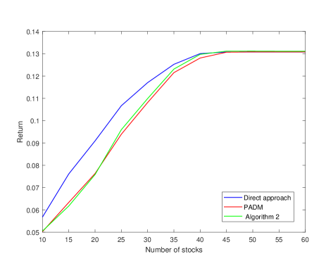
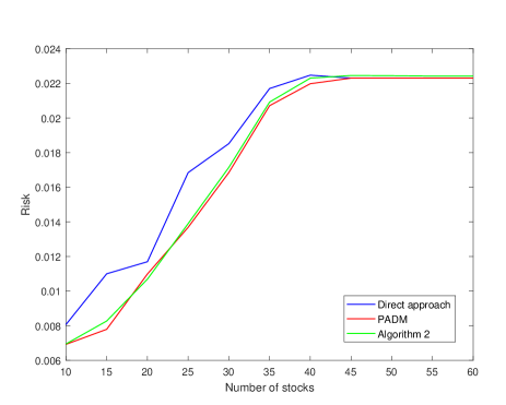
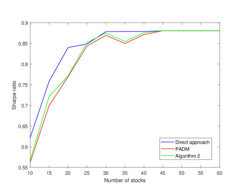
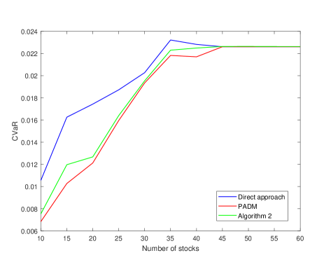
In this section, we compare the performance of Algorithm 2 with the algorithm in [7]. The direct approach of solving ($P$) by CVX-Mosek is also reported for gap computing. We use the data of S&P index for 2018-2021 with 120 stocks when $\lambda_{1}=\lambda_{2}={1}/{3}$, $\phi=0$, $U_{i}=-L_{i}=0.2;\forall i\in[n],\delta=0.002$ and $\beta=0.95$. Moreover, we apply the Geometric Brownian Motion (GBM) model in [1] to generate scenarios. In the PADM algorithm of [7], the initial penalty parameter is set to $1.2$ and it is updated with the factor 3. The inner loop is stopped when $||(x^{s,l},w^{s,l})-(x^{s,l-1},w^{s,l-1})||_{1}\leq 10^{-5}$. It terminates with a partial minimum if $||x-w||_{1}\leq 10^{-5}$. In Algorithm 2, the initial penalty parameter is set to $1.2$ as well and it is updated with the factor 3. In this Algorithm, the inner loop is stopped when $\epsilon_{I}=10^{-5}$ and the outer loop is stopped when a convergence criterion is met $\epsilon_{O}=10^{-5}$. All computations are performed in MATLAB R2017a on a 2.50 GHz laptop with 4 GB of RAM, and CVX 2.2 ([5]) is used to solve the optimization models. The results comparing returns, risks, Sharpe ratios, CVaR values, CPU times, and gaps for different $m$ values are reported in Table 1. The gap in this table is ${|f-\overline{f}|}/{(|f|+1)}$ where $f$ is the return (risk, Sharpe ratio, CVaR) for direct solution approach and $\overline{f}$ is the return (risk, Sharpe ratio, CVaR) for the PADM algorithm or Algorithm 2.

These results show that both Algorithm 2 and PADM are extremely faster than the direct solution approach. Also, Algorithm 2 is about twice as fast as the PADM while having competitive gaps of returns, risks, CVaR, and Sharpe ratios; for all $m$ values. These results for $m=3000$ also are depicted in Figure 1 for different numbers of stocks showing the competitiveness of Algorithm 2. These results confirm that Algorithm 2 is a better alternative to the direct solution approach than the PADM in [7].

5 Conclusion

In conclusion, this paper designs a penalty decomposition algorithm customized for tackling the challenging sparse extended mean-variance-CVaR portfolio optimization problem in finance. This algorithm needs to solve a sequence of penalty subproblems. By employing a block coordinate method, we adeptly exploit every structure in the problem to manage each penalty subproblem, establishing their well-posed nature and deriving closed-form solutions wherever feasible. Our comprehensive convergence analysis demonstrates the efficacy of our introduced algorithm in efficiently reaching a local minimizer of this non-differentiable and nonconvex optimization problem. Furthermore, extensive numerical experiments conducted on real-world datasets validate the practical applicability, effectiveness, and robustness of our introduced algorithm across various evaluation criteria. Overall, this research contributes significantly to the field of portfolio optimization by offering a novel and efficient solution approach with promising practical implications in finance.

Table 1: Comparison of returns, risks, Sharp ratios, CVaR and CPU times for the direct approach, PADM, and Algorithm 2 for different $m$ values for S&P index data with different confidence levels $\beta$ and different number of scenarios $m$ when $\lambda_{1}=\lambda_{2}=\dfrac{1}{3}$, and $k=30$.
$\beta=0.95$
Model m=1000 m=3000 m=5000
Direct approach
Return 0.1202 0.1195 0.1178
Risk 0.0201 0.0188 0.0161
Sharpe ratio 0.8470 0.8728 0.0242
CVaR 0.0191 0.0211 0.0194
CPU time 472.8531 $>$2.0029e+03 $>$ 2.0029e+03
PADM
Return 0.1134 0.1087 0.1109
Risk 0.0169 0.0159 0.0144
Sharpe ratio 0.8709 0.8625 0.9242
CVaR 0.0177 0.0183 0.0217
CPU time 53.2698 119.9078 312.8421
Return gap 0.0060 0.0097 0.0062
Risk gap 0.0031 0.0028 0.0016
Sharpe ratio gap 0.0130 0.0055 0.0030
CVaR gap 7.4739e-04 0.0019 0.0023
Algorithm 2
Return 0.1151 0.1108 0.1111
Risk 0.0173 0.0162 0.0147
Sharpe ratio 0.8755 0.8695 0.9174
CVaR 0.0188 0.0197 0.0224
CPU time 38.4394 58.4394 61.2368
Return gap 0.0045 0.0078 0.0060
Risk gap 0.0028 0.0025 0.0014
Sharpe ratio gap 0.0154 0.0018 0.0065
CVaR gap 3.0090e-04 0.0015 0.0018
Refer to caption
(a)
Refer to caption
(b)
Refer to caption
(c)
Refer to caption
(d)
Figure 1: Comparison of returns, risks, Sharpe ratios, and CVaR for different $k$ values for 130 stocks of S&P index.

References

  • [1] W Farida Agustini, Ika Restu Affianti, and Endah RM Putri. Stock price prediction using geometric brownian motion. In Journal of Physics: Conference Series, volume 974, page 012047. IOP Publishing, 2018.
  • [2] Weichuan Deng, Paweł Polak, Abolfazl Safikhani, and Ronakdilip Shah. A unified framework for fast large-scale portfolio optimization. Data Science in Science, 3(1):2295539, 2024.
  • [3] Jin-Hong Du, Yifeng Guo, and Xueqin Wang. High-dimensional portfolio selection with cardinality constraints. Journal of the American Statistical Association, pages 1–13, 2022.
  • [4] Fernando GDC Ferreira and Rodrigo TN Cardoso. Mean-cvar portfolio optimization approaches with variable cardinality constraint and rebalancing process. Archives of Computational Methods in Engineering, 28(5):3703–3720, 2021.
  • [5] Michael Grant, Stephen Boyd, and Y Ye. Cvx: Matlab software for disciplined convex programming, version 2.0 beta, 2013.
  • [6] Gustavo Grullon, Sébastien Michenaud, and James P Weston. The real effects of short-selling constraints. The Review of Financial Studies, 28(6):1737–1767, 2015.
  • [7] Abdelouahed Hamdi, Tahereh Khodamoradi, and Maziar Salahi. A penalty decomposition algorithm for the extended mean–variance–cvar portfolio optimization problem. Discrete Mathematics, Algorithms and Applications, 16(03):2350021, 2024.
  • [8] Ken Kobayashi, Yuichi Takano, and Kazuhide Nakata. Bilevel cutting-plane algorithm for cardinality-constrained mean-cvar portfolio optimization. Journal of Global Optimization, 81(2):493–528, 2021.
  • [9] AmirMohammad Larni-Fooeik, Hossein Ghanbari, Mostafa Shabani, and Emran Mohammadi. Bi-objective portfolio optimization with mean-cvar model: An ideal and anti-ideal compromise programming approach. In Progressive Decision-Making Tools and Applications in Project and Operation Management: Approaches, Case Studies, Multi-criteria Decision-Making, Multi-objective Decision-Making, Decision under Uncertainty, pages 69–79. Springer, 2024.
  • [10] Man-Fai Leung and Jun Wang. Cardinality-constrained portfolio selection based on collaborative neurodynamic optimization. Neural Networks, 145:68–79, 2022.
  • [11] Zhaosong Lu and Yong Zhang. Sparse approximation via penalty decomposition methods. 2012.
  • [12] Khin T Lwin, Rong Qu, and Bart L MacCarthy. Mean-var portfolio optimization: A nonparametric approach. European Journal of Operational Research, 260(2):751–766, 2017.
  • [13] Hossein Moosaei, Ahmad Mousavi, Milan Hladík, and Zheming Gao. Sparse l1-norm quadratic surface support vector machine with universum data. Soft Computing, 27(9):5567–5586, 2023.
  • [14] Ahmad Mousavi and George Michailidis. Mean-reverting portfolios with sparsity and volatility constraints. arXiv preprint arXiv:2305.00203, 2023.
  • [15] Ahmad Mousavi and George Michilidis. Statistical proxy based mean-reverting portfolios with sparsity and volatility constraints. International Transactions in Operational Research, 2024.
  • [16] Ahmad Mousavi, Mehdi Rezaee, and Ramin Ayanzadeh. A survey on compressive sensing: classical results and recent advancements. Journal of Mathematical Modeling, 8(3):309–344, 2020.
  • [17] Ahmad Mousavi and Jinglai Shen. A penalty decomposition algorithm with greedy improvement for mean-reverting portfolios with sparsity and volatility constraints. International Transactions in Operational Research, 2022.
  • [18] Diana Roman, Kenneth Darby-Dowman, and Gautam Mitra. Mean-risk models using two risk measures: a multi-objective approach. Quantitative Finance, 7(4):443–458, 2007.
  • [19] Pedro AC Saffi and Kari Sigurdsson. Price efficiency and short selling. The Review of Financial Studies, 24(3):821–852, 2011.
  • [20] Yu Shi, Xia Zhao, Xin Yan, et al. Optimal asset allocation for a mean-variance-cvar insurer under regulatory constraints. American Journal of Industrial and Business Management, 9(07):1568, 2019.
  • [21] Ralph E Steuer, Yue Qi, and Maximilian Wimmer. Computing cardinality constrained portfolio selection efficient frontiers via closest correlation matrices. European Journal of Operational Research, 313(2):628–636, 2024.
  • [22] A Taik, R Aboulaich, R Ellaia, and S El Moumen. The mean-variance-cvar model for portfolio optimization modeling using a multi-objective approach based on a hybrid method. Mathematical Modelling of Natural Phenomena, 5(7):103–108, 2010.
  • [23] Pieter M van Staden, Duy-Minh Dang, and Peter A Forsyth. The surprising robustness of dynamic mean-variance portfolio optimization to model misspecification errors. European Journal of Operational Research, 289(2):774–792, 2021.
  • [24] Shuang Wang, Li-Ping Pang, Shuai Wang, and Hong-Wei Zhang. Distributionally robust mean-cvar portfolio optimization with cardinality constraint. Journal of the Operations Research Society of China, pages 1–31, 2023.
  • [25] Siwei Xia, Yuehan Yang, and Hu Yang. High-dimensional sparse portfolio selection with nonnegative constraint. Applied Mathematics and Computation, 443:127766, 2023.
  • [26] Ziping Zhao, Rui Zhou, and Daniel P Palomar. Optimal mean-reverting portfolio with leverage constraint for statistical arbitrage in finance. IEEE Transactions on Signal Processing, 67(7):1681–1695, 2019.