Linguistic Calibration of Language Models

Abstract

Language models (LMs) may lead their users to make suboptimal downstream decisions when they confidently hallucinate. This issue can be mitigated by having the LM verbally convey the probability that its claims are correct, but existing models cannot produce text with calibrated confidence statements. Through the lens of decision-making, we formalize linguistic calibration for long-form generations: an LM is linguistically calibrated if its generations enable its users to make calibrated probabilistic predictions. This definition enables a training framework where a supervised finetuning step bootstraps an LM to emit long-form generations with confidence statements such as “I estimate a 30% chance of…” or “I am certain that…”, followed by a reinforcement learning step which rewards generations that enable a user to provide calibrated answers to related questions. We linguistically calibrate Llama 2 7B and find in automated and human evaluations of long-form generations that it is significantly more calibrated than strong finetuned factuality baselines with comparable accuracy. These findings generalize under distribution shift on question-answering and under a significant task shift to person biography generation. Our results demonstrate that long-form generations may be calibrated end-to-end by constructing an objective in the space of the predictions that users make in downstream decision-making.

1 Introduction

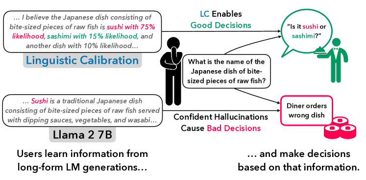
Figure 1: We define linguistic calibration of long-form generations (LC) as calibrating an LM’s long-form generations in a way that leads to calibrated downstream user forecasts. We apply LC to train an LM that emits calibrated statements of confidence in natural language, enabling better downstream decisions. Left: users read long-form generations on a variety of topics, such as Japanese cuisine. Middle: a user faces a decision (what to order). Lower Right: Few-shot prompted Llama 2 7B hallucinates confidently, leading to a suboptimal decision (ordering sushi). Upper Right: Even if the base LM cannot be confidently correct, it can spread probability over possible claims, enabling a better decision.

The claims made by language models (LMs) are increasingly used to inform real-world decisions, e.g., what to order at a restaurant (Fig. 1), what information to provide someone else about a topic, or which code completion to accept. However, LMs have knowledge gaps which manifest as hallucinations Ji et al. (2023), Huang et al. (2023). Currently, when an LM lacks knowledge about a topic, it will do one of two things: hallucinate incorrect claims with complete confidence, or, in the case of a few strong closed-source models OpenAI et al. (2023), Anthropic (2023), abstain from making claims.

Confident hallucinations are especially harmful. They decrease users’ trust in the errant LM and broadly make LMs unsuitable for settings where factuality is paramount such as medicine Thirunavukarasu et al. (2023) and law Dahl et al. (2024). Perhaps most importantly, they lead the user to confidently make poor decisions (Fig. 1 Lower). However, even abstentions are suboptimal, because they provide the user with no plausible claims and their likelihoods.

Linguistic calibration Mielke et al. (2022)—conveying confidence levels in natural language that equal the likelihood that one’s claims are correct—could mitigate the harms of hallucination. If an LM was linguistically calibrated in a manner interpretable to its users, they could make good decisions regardless of the LM’s underlying knowledge.

For example, suppose a clinical LM generates a patient’s case report, providing a diagnosis and treatment plan. If the LM was unsure of the best treatment for a patient, it could use numerical confidence with its corresponding claim (“I estimate that the best treatment is Antibiotic A with 60% confidence”). Then, when the doctor faces a decision—deciding the patient’s treatment—they have access to both a salient claim and an approximate likelihood of its correctness. The manner of conveying confidence is limited only by the use of language: e.g., the LM could provide linguistic confidence statements (“I am fairly sure that the best treatment is A”) or many mutually exclusive claims (“I estimate that the best treatment is A with 60% confidence, though B or C may work better”). However, both classic calibration methods like temperature scaling Guo et al. (2017) and methods for LMs Kadavath et al. (2022), Tian et al. (2023), Kuhn et al. (2023), Mielke et al. (2022), Lin et al. (2022), Jiang et al. (2021) are restricted to classification or short outputs and hence cannot calibrate the many claims made in each long-form LM generation (cf. §5 for related work).

We make progress on this challenge by leveraging the connection between calibration and decision theory Zhao et al. (2021), Zhao and Ermon (2021). LMs fit cleanly within the framework of decision-making. Users query LMs, learn from their generations, and later encounter decision-making tasks with associated questions (“which treatment?”). They forecast an answer based on what they learned, and finally make a decision using their forecast for which they receive some reward.

Because linguistic calibration improves downstream user decisions, we might hope to calibrate an LM by directly optimizing real-world downstream rewards. While intuitively appealing, this process is unsurprisingly challenging; it entails tracing the knowledge learnt by users through to their decisions, and further propagating the associated rewards back to the LM.

Our contributions.

We propose a definition of linguistic calibration for long-form generations (LC) which sidesteps the difficulty of tracing real-world rewards and enables training an LM to emit calibrated confidence statements in long-form generations. Our contributions are as follows:

• We define an LM to be linguistically calibrated if it enables users to produce calibrated forecasts relevant to their decision tasks, which in turn enable optimal decision-making.

• We instantiate this definition in a training objective and framework that calibrates long-form generations through a decision-theoretic lens. Our training framework first bootstraps an LM to express confidence statements with supervised finetuning. Then, it optimizes our objective using reinforcement learning (RL), rewarding the LM policy for generating text that enables calibrated forecasts on related questions.

• We linguistically calibrate Llama 2 7B using our training framework and find it significantly improves calibration versus strong baselines finetuned for factuality while matching their accuracy, in human and API-based LLM evaluation of long-form generations. We also show that linguistic calibration has zero-shot transfer beyond the training task. Specifically, an LM calibrated using a single off-the-shelf question-answering dataset is also calibrated on out-of-distribution question-answering datasets, and on an entirely held-out task of biography generation.

Instead of working in the space of text, our decision-based approach constructs an objective in the space of the predictions that users make in the process of decision-making. This makes the standard calibration machinery of proper scoring rules Gneiting and Raftery (2007) tractable as an objective for end-to-end calibration of long-form generations.

2 Preliminaries

Our goal is to formulate a tractable objective that enables the end-to-end linguistic calibration of long-form LM generations. To begin, we give a formal framework for how LMs factor into the decisions of users. Then we will be able to define what it means for an LM to be linguistically calibrated and construct an objective to optimize for it.

2.1 User Decision Problem

Users learn about a variety of topics by reading LM generations: for example, doing research, planning trips, or reviewing clinical notes. Long-form generations in particular are increasingly ubiquitous and useful. Instead of needing to prompt an LM with many precise questions, users can quickly accumulate knowledge by providing LMs with open-ended queries. Then, they can use this knowledge to make predictions which inform decisions. We will formalize this process as decision-making based on probabilistic forecasts Zhao and Ermon (2021).

Decision-making with LM assistance.

In decision-making with LM assistance, the user first prompts an LM $\pi$ with an open-ended query $q$ (“Generate a clinical note for this patient…”). The LM generates a long-form context $z\sim\pi(z\mid q)$ which the user learns from: e.g., the doctor reads the LM-generated clinical note about the patient’s condition. Next, at some point in the future, the user encounters a decision task which is related to the context $z$: e.g., they need to decide on a treatment for the patient. More precisely, the user needs to select an action $a\in\mathcal{A}$ (which treatment to provide the patient). Any decision task has an associated question $x$ (“Which treatment should the patient take?”) with answer $y$ (“Antibiotic A”), so we associate each decision task with a question-answer pair $(x,y)\sim p(x,y)$. The true distribution over answers $p(y\mid x)$ is unknown to the user.

In order to make a decision, the user first forms a probabilistic forecast over possible answers. Because the LM’s long-form context $z$ is relevant to this decision task, the user conditions on it to form forecast $\widehat{p}(y\mid x,z)$. Now, the user can choose an action $a\in\mathcal{A}$ according to this forecast and a loss function $L:(\mathcal{A},\mathcal{Y})\rightarrow\mathbb{R}$. For example, the user may make a Bayes-optimal decision by choosing the action which minimizes their loss under the forecast distribution $a^{*}=\operatorname*{arg\,min}_{a}\mathbb{E}_{\widehat{y}\sim\widehat{p}(y\mid x,z)}[L(a,\widehat{y})]$. Based on the realized answer $y\sim p(y\mid x)$, the user suffers a loss of $L(a^{*},y)$.

2.2 Linguistic Calibration by Calibrating Generations to Forecasts

Ideally, one would follow this LM-assisted process and directly train an LM to generate contexts $z$ which minimize the user’s downstream loss $L(a^{*},y)$. However, it is difficult to obtain real-world rewards from decision-making, and moreover to obtain a real-world distribution over queries to LMs and related user decision tasks $p(q,x,y)$. To overcome these challenges, we make two approximations. First, instead of measuring downstream losses $L(a^{*},y)$, we will construct a surrogate loss $\ell(z;x,y)$ in the form of a proper scoring rule Gneiting and Raftery (2007) of the user’s probabilistic forecast over answers $\widehat{p}(y\mid x,z)$. Intuitively, optimizing this objective will encourage the LM to generate contexts $z$ that enable users to provide calibrated answers to decision task questions $x$. Second, we will switch to a surrogate distribution over decision tasks; we use knowledge-intensive question-answering datasets to generate a set of user decision tasks.

In the rest of this section, we focus on the surrogate loss, demonstrating optimality properties which make it a reasonable approximation. We discuss our surrogate decision task distribution in §3.1.

Optimizing long-form generations for linguistic calibration.

By construction, our surrogate loss $\ell(z;x,y)$ is independent of the action $a$ and the downstream losses $L(a^{*},y)$, meaning we sidestep the challenge of tracing real-world decisions and losses. Nonetheless, if user forecasts are calibrated, we are in fact guaranteed that decision-making based on those forecasts is optimal in a certain sense Zhao et al. (2021). Specifically, we will show the following guarantee: if we can minimize our objective $\ell(z;x,y)$, we will also minimize the user’s downstream loss $L(a^{*},y)$. This provides us a definition of linguistic calibration that applies to long-form generations (LC):

Prior work defines linguistic calibration in the context of single-claim utterances, considering a linguistically calibrated LM to be one that emits verbalized confidence statements matching the likelihood of a response’s correctness Mielke et al. (2022). However, the long-form, multi-claim generations that users encounter in practice have neither a single closed-form confidence nor a correctness; each generation contains information that answers many possible downstream questions. Our definition generalizes linguistic calibration to long-form generations by explicitly defining it with respect to downstream users and their LM-assisted forecasts $\widehat{p}(y\mid x,z)$. This work focuses on calibrating long-form text, and therefore any future uses of the terms linguistic calibration, linguistically calibrated, etc. refer to the definition above.

Training framework.

Our definition is also actionable; we will instantiate a scalable training framework to linguistically calibrate an LM by simulating user forecasts with neural net surrogate forecasts. Then we may optimize our objective $\ell(z;x,y)$ end-to-end, training the LM to emit contexts $z$ that lead to calibrated surrogate forecasts.

We will next explain why optimizing $\ell(z;x,y)$ is a reasonable proxy to directly optimizing downstream losses $L(a^{*},y)$, using a connection between calibration and decision-making. Then we will be able to state our objective for linguistic calibration.

2.3 Calibration and Decision-making

Calibration implies that Bayes-optimal decisions are zero expected regret.

Zhao et al. (2021) prove correspondences between the calibration of forecasts and zero regret strategies under a Bayes-optimal decision-maker. This theoretical connection motivates our approach of calibrating user forecasts; optimizing $\ell(z;x,y)$ is a sensible proxy to directly optimizing losses $L(a^{*},y)$. At the same time, by formulating our objective in the space of probabilistic forecasts instead of in the space of text, we may now employ standard calibration techniques for classification settings. More concretely, our objective calibrates forecasts $\widehat{p}(y\mid x,z)$ using proper scoring rules, which we review next.

Proper Scoring Rules Gneiting and Raftery (2007).

Scoring rules measure the quality of a forecast. A scoring rule for forecast $\widehat{p}\in\Delta$ of a categorical variable $Y$ is a function $R:(\Delta,\mathcal{Y})\rightarrow\mathbb{R}$, i.e., with forecast $\widehat{p}$ and outcome $y$, the forecaster’s reward is $R(\widehat{p},y)$. If a scoring rule is proper, it has the desirable property that it is maximized when the forecaster predicts the true probability, i.e., $\widehat{p}=p$. Formally, $R$ is proper if

$$\mathbb{E}_{Y\sim p}[R(p,Y)]\geq\mathbb{E}_{Y\sim p}[R(\widehat{p},Y)],\;~{}\forall p,\widehat{p}\in\Delta.$$

$R$ is strictly proper if the unique maximizer of the expected reward is the true probability $p$. Strictly proper scoring rules are ubiquitous in ML, e.g., the (negative) log loss or Brier score Brier (1950), and are natural objectives for calibration methods such as temperature Guo et al. (2017) or Platt scaling Platt et al. (1999).

2.4 Linguistic Calibration Objective

Altogether, our surrogate loss is a strictly proper scoring rule of the user forecast:

$$\ell(z;x,y):=-R(\widehat{p}(\cdot\mid x,z),y),$$

where $R$ is strictly proper. We optimize this objective to linguistically calibrate an LM with the following guarantee: if we maximize $R(\widehat{p}(\cdot\mid x,z),y)$, then the user’s forecast $\widehat{p}(y\mid x,z)$ is perfectly calibrated, because it equals the ground-truth $p(y\mid x)$. Then, by the equivalence of calibration and optimal decision-making Zhao et al. (2021), a user making Bayes-optimal decisions will incur zero expected regret against all other decision rules.

Guarantees for weaker notions of calibration.

Of course, it is unreasonable to expect that we can perfectly maximize $R(\widehat{p}(\cdot\mid x,z),y)$. Nonetheless, we still obtain guarantees if we achieve linguistic calibration with respect to a weaker calibration metric $\phi$, i.e., the user’s forecast $\widehat{p}(y\mid x,z)$ is calibrated in a weaker sense. For example, consider confidence calibration, a common notion of a classifier’s calibration in the deep learning literature Guo et al. (2017), Minderer et al. (2021). Confidence calibration means that among the examples with top forecasted probability equal to $\beta$, the accuracy over those examples is also $\beta$; i.e., for all $\beta\in[0,1]$,

$$\Pr\left(Y=\operatorname*{arg\,max}_{y}\widehat{p}(y\mid x)\mathrel{\Big{|}}\max_{y}\widehat{p}(y\mid x)=\beta\right)=\beta.$$

We apply the results of Zhao et al. (2021) to demonstrate the following no-regret guarantee. Let $\phi_{\text{cc}}$ be the confidence calibration metric. Suppose that an LM is $\phi_{\text{cc}}$-linguistically calibrated with respect to a user (i.e., the user has confidence calibrated forecasts $\widehat{p}(y\mid x,z)$), and that the user has loss function $L$ from a certain family of losses $\mathcal{L}_{\text{r}}$. Then if the user acts Bayes-optimally, they will perform no worse than many other decision rules. Appendix B provides a formal statement and proof of this guarantee (Proposition B.5), along with a formal definition of linguistic calibration and discussion on other benefits of linguistic calibration for decision-making.

Lastly, we note that this connection between confidence calibration and optimal decision-making motivates our evaluation metric of forecast expected calibration error (defined in §4.1).

We proceed by discussing our training framework (§3), experimental results (§4), related work (§5), and lastly, limitations, future work, and conclusions (§6).

3 Method

Our procedure for linguistically calibrating an LM begins by constructing a surrogate distribution that approximates the real-world distribution of user decision tasks. Then, we apply a two-step training framework (Fig. 2). First, we obtain an LM with some ability to express confidences in a long-form generation. Second, we use it as an RL policy and optimize our proper scoring rule objective end-to-end, with supervision from the surrogate task distribution.

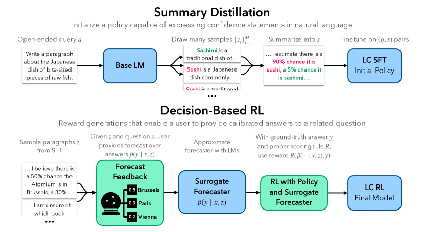
Figure 2: Our training framework for linguistic calibration of long-form generations (LC) calibrates the long-form generations of an LM by calibrating downstream user forecasts. It involves two steps: summary distillation (Upper) and decision-based RL (Lower). Datasets are in white, LMs in blue, and steps involving user or surrogate forecasts are in green.

3.1 Generating Supervision for Long-Form Calibration

In our setup (§2.1), the process of user decision-making with LM assistance involves a tuple $(q,z,x,y)$, where $q$ are user-written queries to the LM, $z\sim\pi(z\mid q)$ are long-form generations sampled from the LM, and $(x,y)$ is a related question-answer pair that specifies a real-world user decision task.

Our training framework will closely follow this process and therefore requires access to a dataset of tuples $(q,z,x,y)$. We will synthetically generate this dataset in a manner agnostic to any downstream task, making use of arbitrary question-answer pairs $(x,y)$. In this work, we make a particular choice to use $(x,y)$ pairs from off-the-shelf question-answering datasets.

Specifically, we use the following synthetic data generation process. First, we sample a question-answer pair $(x,y)\sim p(x,y)$ from a question-answering dataset, which implicitly specifies some actual decision task. Next, we need an LM query $q$ such that $z\sim\pi(z\mid q)$ is a long-form generation salient to $(x,y)$. We obtain one by taking the question $x$ and converting it into an open-ended query ($q:=$ “Write a paragraph about {$x$}”) using an API-based LLM. Altogether, this gives us a tuple $(q,z,x,y)$ where $(q,x,y)\sim p(q,x,y)$ and $z\sim\pi(z\mid q)$. We henceforth use this notation.

Next, we describe our two-step training framework.

3.2 Summary Distillation

Summary distillation (Fig. 2 Upper) bootstraps a base LM $\pi_{\text{Base}}$ to have some ability to express its confidence in long-form natural language generations. We follow a simple approach inspired by Self-Consistency Wang et al. (2023), which obtains calibrated LM confidences for short answer questions by computing a statistic of many output samples. Summary distillation generalizes this idea to longer generations, and then finetunes on our equivalent of the statistics.

First, we provide the base LM with an open-ended query $q$ and sample many long-form responses: $\{z_{i}\}_{i=1}^{M}\sim\pi_{\text{Base}}(z\mid q)$. To obtain statements of confidence that are faithful to the base model’s internal confidence levels, we prompt an API-based LLM to summarize these samples into a single consensus paragraph $s$ with statements of confidence based on the frequency of claims: $s\sim\text{Summarize}(s\mid z_{1},\dots,z_{M})$. For example, we would expect the summary shown in Fig. 2 (Upper) if $90\%$ of the $M$ samples answer the question with Sushi and $5\%$ with Sashimi. We perform frequency-based summarization at the claim level, meaning that each summary paragraph $s$ contains multiple claims with various confidence levels and styles (e.g., numerical and linguistic).

Finally, to distill these extracted confidences back into the base model, we finetune $\pi_{\text{Base}}$ on the dataset of open-ended query and summary pairs $\{(q^{(i)},s^{(i)})\}_{i=1}^{N}$ to obtain the supervised finetuned (SFT) model $\pi_{\text{SFT}}$. $\pi_{\text{SFT}}$ serves as a strong initial policy for the second RL-based step.

3.3 Decision-Based RL

Decision-based RL (Fig. 2 Lower) linguistically calibrates a policy $\pi_{\text{RL}}$ (initialized at $\pi_{\text{SFT}}$) by finetuning it to emit long-form generations $z$ that improve the calibration of a user forecast $\widehat{p}(y\mid x,z)$.

Reward function.

Following our discussion on scoring rules (§2.3), any strictly proper scoring rule is a suitable choice as a reward function to encourage calibration of the forecast $\widehat{p}(y\mid x,z)$. We simply choose the log likelihood:

$$R_{\texttt{LC}}(\widehat{p}(\cdot\mid x,z),y^{\prime}):=\log\widehat{p}(y^{\prime}\mid x,z).$$ (1)

RL objective.

Our RL objective, which optimizes rewards over our semi-synthetic distribution, is

$$\max_{\pi_{\text{RL}}}\underset{(q,x,y)\sim p(q,x,y),~{}z\sim\pi_{\text{RL}}(z\mid q)}{\mathbb{E}}\left[R_{\texttt{LC}}\left(\widehat{p}(\cdot\mid x,z),y\right)\right].$$ (2)

3.4 Implementation

We next describe our instantiation of decision-based RL, which we used in our experiments. However, we note that the notion of linguistic calibration defined in §2 is agnostic to these design decisions. Algorithm 1 presents the pseudocode.

Given: SFT LM $\pi_{\text{SFT}}$, LLM forecaster $\widehat{p}_{\text{LLM}}(y\mid x,z)$, decision task joint distribution $p(q,x,y)$.

Result: linguistically calibrated LM $\pi_{\texttt{LC}}$.

/* Construct datasets for training surrogate forecaster functions: */

/*     ExtractAnswers (EA) and ForecastProbs (FP). */

$\mathcal{D}_{\text{EA}}\leftarrow\{\},\mathcal{D}_{\text{FP}}\leftarrow\{\}$.

for i = 1, …, N do

       /* LM-assisted user decision-making, up to forecast step. */

       Sample open-ended query and decision task: $(q,x,y)\sim p(q,x,y)$.

       Sample long-form generation $z\sim\pi_{\text{SFT}}(z\mid q).$

       Obtain API-based LLM forecast $\widehat{p}_{\text{LLM}}(\cdot\mid x,z)$.

       /* Add ExtractAnswers example. */

       $\mathcal{D}_{\text{EA}}\leftarrow\mathcal{D}_{\text{EA}}\cup\Big{(}x,z,\text{Support}(\widehat{p}_{\text{LLM}}(\cdot\mid x,z))\Big{)}$.

       /* Add ForecastProbs example for ground-truth answer. */

       $\mathcal{D}_{\text{FP}}\leftarrow\mathcal{D}_{\text{FP}}\cup\Big{(}x,z,y,\widehat{p}_{\text{LLM}}(y\mid x,z)\Big{)}$.

       /* Add ForecastProbs example for all extracted answers. */

       for extracted answer $y^{\prime}\in\text{Support}(\widehat{p}_{\text{LLM}}(\cdot\mid x,z))$ do

             $\mathcal{D}_{\text{FP}}\leftarrow\mathcal{D}_{\text{FP}}\cup\Big{(}x,z,y^{\prime},\widehat{p}_{\text{LLM}}(y^{\prime}\mid x,z)\Big{)}$.

            

       end for

      

end for

/* Finetune surrogate LMs. */

  Finetune ExtractAnswers on $\mathcal{D}_{\text{EA}}$ and ForecastProbs on $\mathcal{D}_{\text{FP}}$.

/* Optimize RL objective. */

$\pi_{\texttt{LC}}\leftarrow$ PPO with initial policy $\pi_{\text{SFT}}$, surrogate forecaster $\widetilde{p}$, and Objective 3.

return $\pi_{\texttt{LC}}$

Algorithm 1 Decision-Based RL with a Surrogate Forecaster

Surrogate forecaster.

For our training framework to be as scalable as possible, we would ideally avoid the use of user forecasting (both human and LLM-simulated) in the RL loop. We find that we can train a neural net surrogate forecaster $\widetilde{p}(y\mid x,z)$ which produces reasonable forecasts, because forecasting conditional on $z$ is not a fundamentally challenging task. For example, if $z$ provides a clear list of possible answers to the question $x$ and associated percentage likelihoods, forecasting is a simple extractive task.

Using the surrogate, we optimize approximate reward $R_{\texttt{LC}}(\widetilde{p}(\cdot\mid x,z),y)\approx R_{\texttt{LC}}(\widehat{p}(\cdot\mid x,z),y)$. In our evaluation, we will test if our LM calibrated on this approximate reward generalizes to produce long-form generations $z$ which improve simulated LLM and human forecasts $\widehat{p}(y\mid x,z)$.

We cannot simply train a neural net to directly predict a softmax output $\widetilde{p}(y\mid x,z)$, because $\mathcal{Y}$ is the vast space of all answers expressible in a finite-length string. Instead, we decompose forecasting into two operations:

1. ExtractAnswers: $(x,z)\mapsto\text{ExtractAnswers}(x,z)\subset\mathcal{Y}$, which extracts all possible answers to the question $x$ from the paragraph $z$. We implement this by finetuning a pretrained LM (RedPajama 3B, together.ai (2023)).

2. ForecastProbs: $(x,z,y^{\prime})\mapsto[0,1]$, which assigns a probability value to an answer $y^{\prime}$ to question $x$ based on the paragraph $z$. We implement this by finetuning $\pi_{\text{SFT}}$ with a cross-entropy loss.

We define the surrogate forecast $\widetilde{p}(y|x,z)$ as a categorical distribution with probability $\text{ForecastProbs}(x,z,y^{\prime})$ on each answer $y^{\prime}\in\text{ExtractAnswers}(x,z)$, and probability 0 on all others. In this particular construction, we are not guaranteed that the surrogate forecast $\widetilde{p}(y\mid x,z)$ will be normalized, but in practice we find that adding a regularization term is sufficient to enforce normalization:

$$R_{\texttt{LC}}(\widetilde{p}(\cdot\mid x,z),y^{\prime})= \log\widetilde{p}(y^{\prime}\mid x,z)\!-\!\lambda\left|1\!-\!\textstyle\sum_{y\in\mathcal{Y}}\widetilde{p}(y\mid x,z)\right|,$$

where $\lambda>1$ restores strict propriety (cf. C.1 for proof). Lastly, we use a standard KL penalty from $\pi_{\text{SFT}}$ to mitigate over-optimization of the surrogate forecaster Ouyang et al. (2022), giving us the following objective (where $\beta$ is the KL reward coefficient):

$$\max_{\pi_{\text{RL}}}\underset{(q,x,y)\sim p(q,x,y),~{}z\sim\pi_{\text{RL}}(z\mid q)}{\mathbb{E}}\left[R_{\texttt{LC}}(\widetilde{p}(\cdot\mid x,z),y)-\beta\log\frac{\pi_{\text{RL}}(z\mid q)}{\pi_{\text{SFT}}(z\mid q)}\right].$$ (3)

See Appendix C for further implementation details.

4 Experiments

This section empirically validates our training and evaluation framework for linguistic calibration, demonstrating that it fulfills the following three goals:

1. LC provides better calibration with comparable accuracy. We show that our linguistically calibrated LM $\pi_{\texttt{LC}}$ emits long-form generations $z$ which improve the calibration of user forecasts with accuracy comparable to strong baselines finetuned for factuality with RL.

2. LC is computationally tractable. We show that $\pi_{\texttt{LC}}$—which avoids the need to obtain many costly human forecasts by training with cheap surrogates—improves the calibration of human forecasts at evaluation time. Moreover, we develop an automated framework to evaluate linguistic calibration with simulated forecasts and validate its agreement with crowdworkers.

3. LC generalizes well out-of-distribution. We demonstrate that the improvement in forecast calibration due to adopting LM $\pi_{\texttt{LC}}$ generalizes under a shift in the decision task distribution $(x,y)\sim p_{\text{OOD}}(x,y)$, where $p_{\text{OOD}}(x,y)\neq p(x,y)$. We also evaluate $\pi_{\texttt{LC}}$ on an entirely held-out task of person biography generation, finding that $\pi_{\texttt{LC}}$ produces calibrated claims throughout the long-form generation $z$ according to a fine-grained simulated evaluation.

4.1 Setup

We use our training framework to linguistically calibrate Llama 2 7B, with TriviaQA Joshi et al. (2017) as a source of decision task question-answer (QA) pairs $(x,y)$ (cf. §3.1). We emphasize that our LMs produce long-form generations $z$ on the question’s topic, unlike previous works which calibrate models that directly predict a class distribution or short answer (cf. §5). We refer the reader to Appendix C for further details on the training framework.

Question-answering evaluation framework.

Following our generative process during training (§3.1), we use off-the-shelf QA datasets as a proxy for real-world decision tasks, and evaluate the linguistic calibration of generations $z$ through the performance of downstream forecasts. Specifically, for a held-out decision task $(x,y)$, we convert $x$ into an open-ended query $q$, sample a long-form generation $z\sim\pi(z\mid q)$ from various LMs $\pi$, and evaluate the calibration and accuracy of forecast $\widehat{p}(y\mid x,z)$.

Naturally, this framework depends on which users are providing forecasts and how. We are interested in the case where users strongly rely on the knowledge of the LM. Therefore, we include instructions to the user (either simulated or human) to ignore their background knowledge about the correct answer when providing a forecast (cf. Appendix D for further evaluation details).

Forecast Expected Calibration Error.

We measure the calibration of LM-assisted forecasts $\widehat{p}(y\mid x,z)$ with Expected Calibration Error (ECE) Guo et al. (2017). Intuitively, forecast ECE is a proxy for decision-making performance through the equivalence of confidence calibration and optimal decision-making: see Proposition B.5 in Appendix B for details. Given $N$ question-answer pairs $\{(x^{(i)},y^{(i)})\}_{i=1}^{N}$ and corresponding long-form generations $\{z^{(i)}\}_{i=1}^{N}$, we partition them into $M$ bins by max forecast probability $\max_{y}\widehat{p}(y\mid x^{(i)},z^{(i)})$. ECE is then expressed as

$$\text{ECE}=\sum_{j=1}^{M}\frac{|B_{j}|}{N}\left|\text{Acc}(B_{j})-\text{Conf}(B_{j})\right|,\quad\text{where}$$

$$\text{Conf}(B_{j})=\frac{1}{|B_{j}|}\sum_{i\in B_{j}}\max_{y}\widehat{p}(y\mid x^{(i)},z^{(i)}),\quad~{}\text{Acc}(B_{j})=\frac{1}{|B_{j}|}\sum_{i\in B_{j}}\mathbbm{1}[y^{(i)}=\operatorname*{arg\,max}_{y}\widehat{p}(y\mid x^{(i)},z^{(i)})].$$

We set the number of bins as $M=20$ on simulated QA evaluations, and $M=10$ on all others. Note that log loss is not a reasonable evaluation metric in our setting because simulated and human forecasters can assign zero probability to the ground-truth class label resulting in infinite log loss.

Baselines.

In our main evaluations, we compare LC RL ($\pi_{\texttt{LC}}$) with two types of baselines, all derived from Llama 2 7B: non-confidence and confidence. We provide a strong data-matched comparison to LC by finetuning directly for factuality using RL. This baseline is similar to Tian et al. (2024), but instead of using self-supervised or automated factuality scores as the RL reward, we use correctness determined with ground-truth question-answer pairs from TriviaQA. In-context learning (ICL) baselines use TriviaQA examples from a prompt development split, and SFT/RL-based baselines use the same splits as $\pi_{\text{SFT}}$ and $\pi_{\texttt{LC}}$. Each example in our splits is a $(q,x,y)$ tuple, where $q$ is an open-ended query obtained from question $x$ (cf. §3.1).

We include the following non-confidence baselines:

• ICL. We randomly sample 8 open-ended queries, generate long-form responses with GPT-4, manually fact-check those responses using Wikipedia, and use these fact-checked (query, response) pairs as ICL examples for Llama 2 7B.

• Claude Distill. We generate long-form responses with Claude 2 over all queries in the SFT split, and finetune Llama 2 7B on these (query, response) pairs.

• Factuality SFT. We use the above ICL baseline to generate long-form responses over all queries in the SFT split, and finetune Llama 2 7B on these (query, response) pairs. We found Factuality SFT to outperform Claude Distill on a validation split, so we use it as the starting point for the following baseline, Factuality RL.

• Factuality RL. To provide a strong RL-based baseline, we train a reward model which scores the correctness of long-form outputs and use it in RL. Our approach for obtaining this baseline is analogous to the decision-based RL algorithm (Algorithm 1), except instead of training surrogate forecasters, we train a single reward model that, given a generation $z$ and question-answer pair $(x,y)$, predicts a binary indicator whether $z$ provides the correct answer to the question. This serves as the RL reward. We use Factuality SFT as the initial policy for PPO.

When training our confidence methods, we use the ICL baseline above to generate the responses which are summarized in summary distillation. Our confidence baselines include the LC SFT model ($\pi_{\text{SFT}}$) and the following baseline:

• Summary ICL. We use the summary distillation algorithm (§3.2) on 8 queries sampled from the prompt development split to produce 8 Claude 2 summaries $\{s^{(i)}\}_{i=1}^{8}$, which we use in (query, summary) ICL examples.

Other baselines including GPT-4.

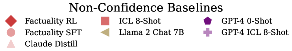
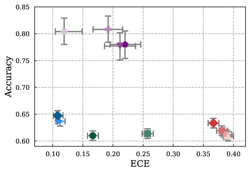
Figure 8: Accuracy-ECE Frontier for All Methods on TriviaQA, evaluated with simulated forecaster (upper left is better). GPT-4 Summary ICL works well despite its simplicity. LC RL outperforms all methods in ECE, including GPT-4 Summary ICL and Direct Summary Eval. Llama 2 Chat 7B performs significantly worse than all other methods and is not displayed for clarity (cf. Table 1 for all numerical results).

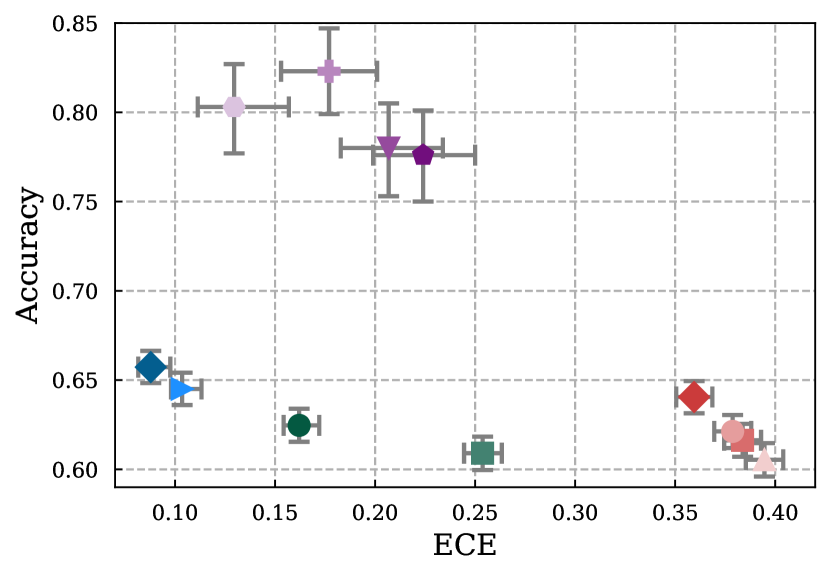
Figure 10: Accuracy-ECE Frontier for All Methods on Jeopardy, evaluated with simulated forecaster (upper left is better). Results are similar to TriviaQA. GPT-4 Summary ICL works well despite its simplicity. LC RL outperforms all methods in ECE, including GPT-4 Summary ICL and Direct Summary Eval. Llama 2 Chat 7B performs significantly worse than all other methods and is not displayed for clarity (cf. Table 1 for all numerical results).

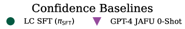
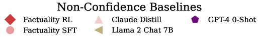
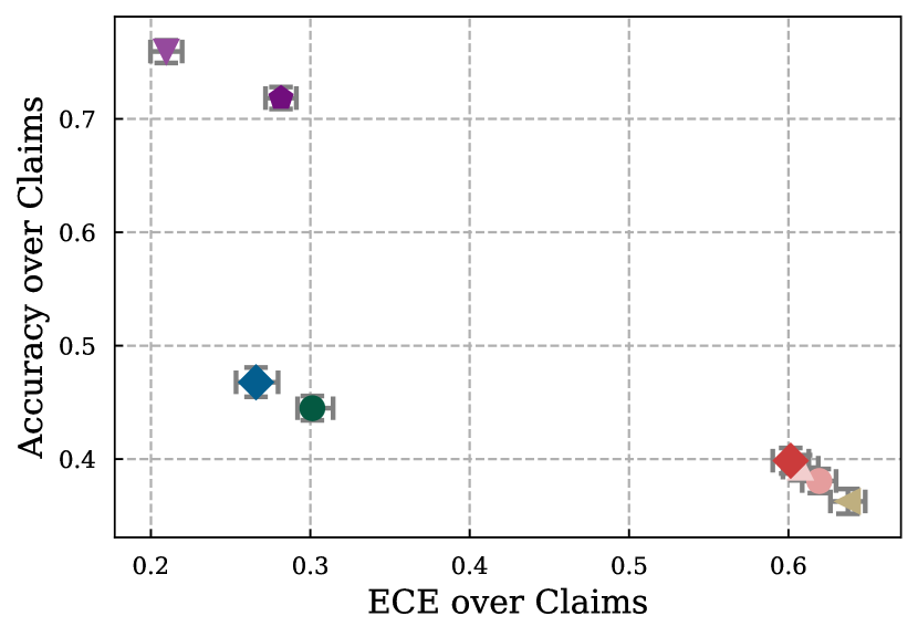
Figure 12: Accuracy-ECE Frontier for All Methods on Person Biography Generation, evaluated with simulated forecaster (upper left is better). GPT-4 is a strong baseline, and GPT-4 Just Ask for Uncertainty (JAFU) does improve both accuracy and ECE. Notably, LC RL has better ECE than GPT-4 0-Shot, despite being trained from a Llama 2 7B base model.

We include results for several other methods in Appendix A including Llama 2 Chat (which underperformed Factuality SFT), the oracle baseline of direct evaluation of summaries $s$, and GPT-4–based methods including GPT-4 0-Shot, GPT-4 ICL 8-Shot, asking GPT-4 for confidence statements zero-shot, and Summary ICL using GPT-4. Unsurprisingly, GPT-4–based methods are far more factual than all Llama 2 7B–based methods. However, we find that LC RL has forecast ECE comparable to GPT-4 baselines (cf. Figs. 8, 10, 12), despite significantly worse factuality. This demonstrates that even small LLMs with relatively weak factuality can be well-calibrated with the right objective.

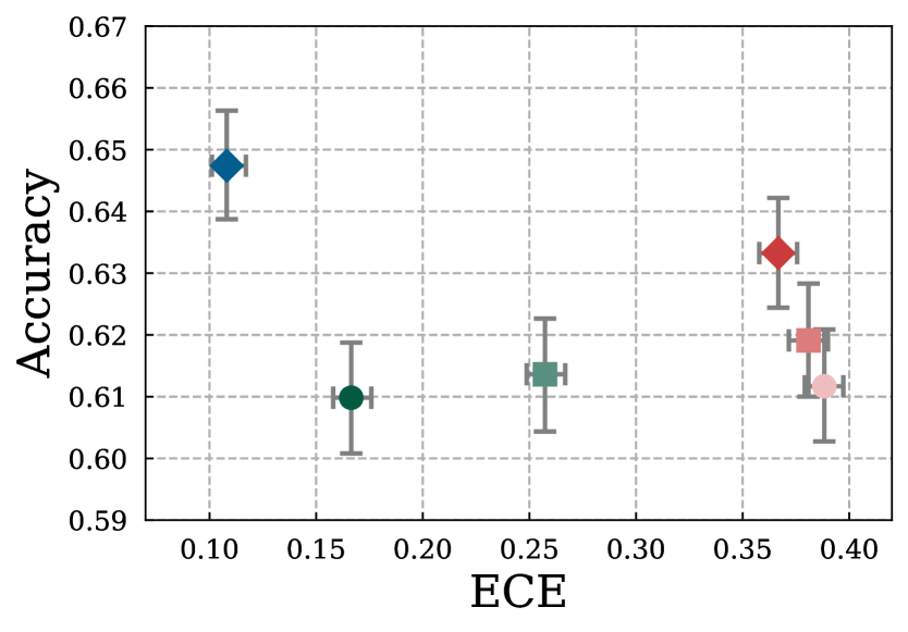
(a) TriviaQA (in-distribution),
 simulated forecaster.

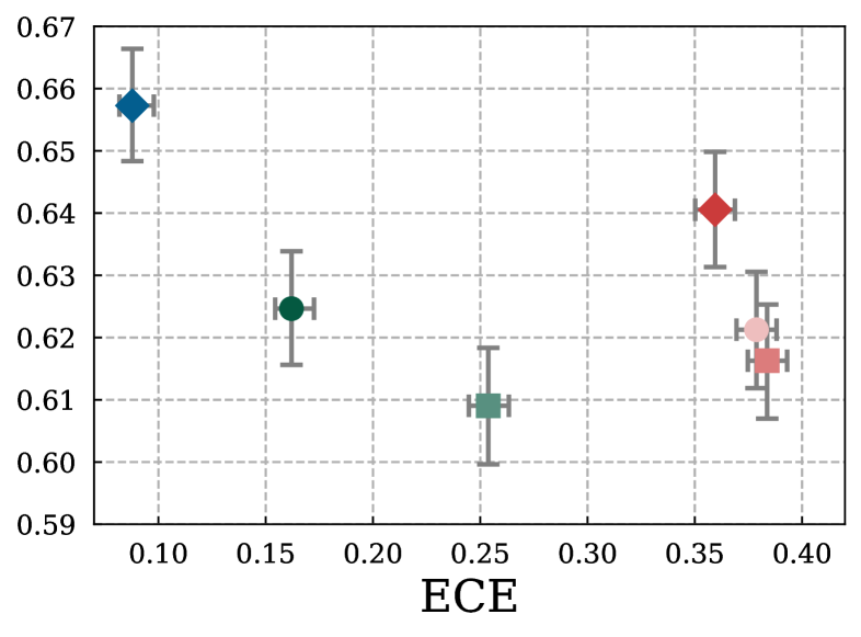
(b) Jeopardy (out-of-distribution),
 simulated forecaster.

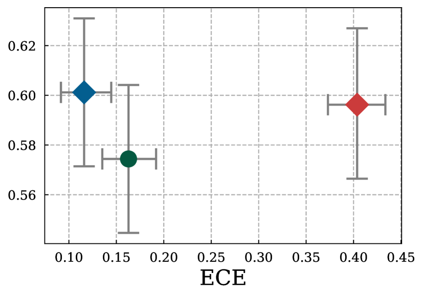
(c) TriviaQA (in-distribution),
 human forecaster.

Figure 3: Accuracy-ECE Frontier for Question-Answering (upper left is better). LC RL pareto-dominates Factuality RL and SFT, with significantly better forecast ECE while matching or exceeding their accuracy.

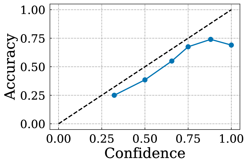
(a) LC SFT, human
forecasters. ECE: $0.163$

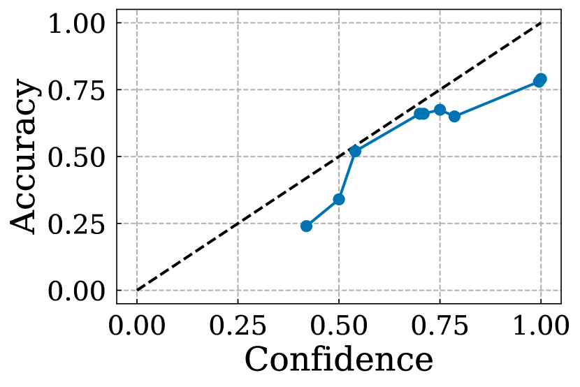
(b) LC RL, human
forecasters. ECE: $0.116$

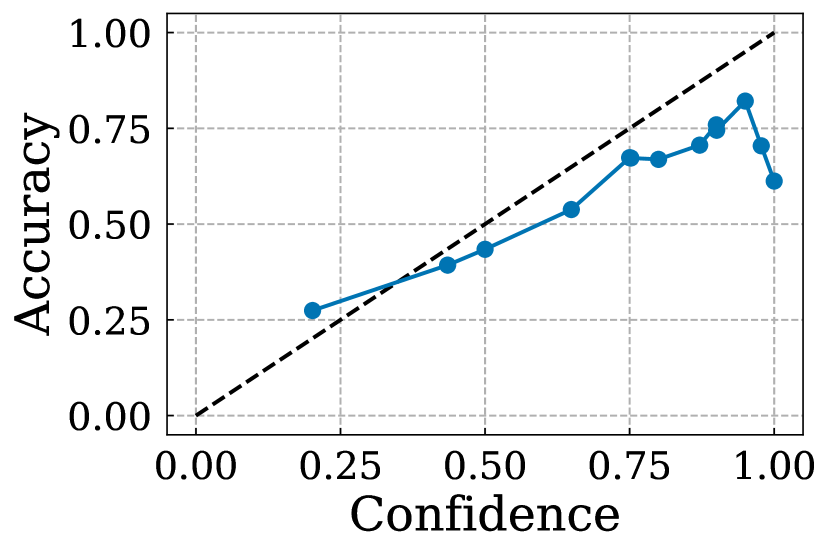
(c) LC SFT, simulated
forecaster. ECE: $0.166$

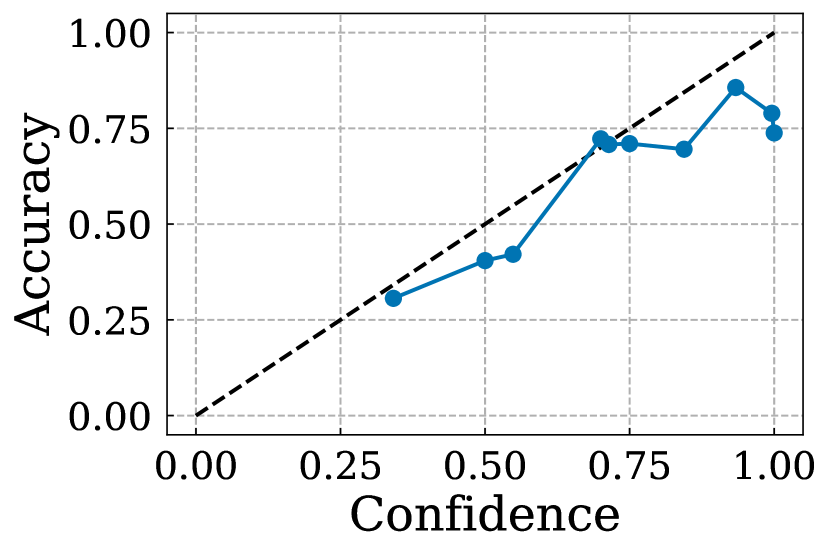
(d) LC RL, simulated
forecaster. ECE: $0.108$

Figure 4: TriviaQA Reliability Diagrams. LC models display a wide range of confidences and good calibration in their long-form generations, with LC RL improving calibration further. Human and simulated results closely match.

4.2 Linguistic Calibration using Question-Answering Datasets

To begin, we evaluate our methods using held-out $(x,y)$ pairs from the TriviaQA and Jeopardy Kaggle (2020) question-answering datasets as decision task examples. These QA evaluations validate two of our three goals: we find that LC improves calibration without compromising accuracy, and that our training and evaluation framework are computationally tractable. Our strong results on the Jeopardy dataset also provide a partial validation of our final goal of strong generalization under distribution shift. Throughout QA evaluations, we use simulated evaluation test sets with more than $10$k examples and human test sets with more than $1$k examples.

Better ECE with comparable accuracy in long-form generation.

Our main result in Fig. 3 is that LC RL has significantly better ECE than non-confidence baselines, including Factuality RL, while matching or exceeding their accuracy. This result holds in-distribution on TriviaQA with both simulated (Fig. 3(a)) and human (Fig. 3(c)) forecasters, and on the out-of-distribution (OOD) Jeopardy dataset (Fig. 3(b)) with a simulated forecaster, demonstrating that LC generalizes across distribution shifts in the decision task distribution $p(x,y)$.

Our results also support the effectiveness of decision-based RL. LC RL significantly improves over LC SFT in both ECE and accuracy, with a greater absolute improvement in ECE/accuracy than Factuality SFT to Factuality RL. This supports our claim that optimizing proper scoring rules of downstream forecasts is an effective way to induce calibration in long-form generations.

Prompt: Write a paragraph bio about Rory Byrne.

Figure 5: Qualitative example from Factuality and LC RL when evaluated under task distribution shift on biography generation. LC RL produces numerical and linguistic confidence statements throughout the paragraph, highlighted in blue. False statements are highlighted in red. We include additional examples in Appendix A.8.

Reliability diagrams demonstrate meaningful confidences.

A natural question is whether the confidences learned by our LC models are meaningful. For example, if all confidences of a model collapsed to its average accuracy, it would obtain perfect ECE despite having confidences that are useless for tasks such as conveying the likelihood of hallucination. To obtain a more fine-grained understanding of a model’s calibration, we use reliability diagrams DeGroot and Fienberg (1983), Niculescu-Mizil and Caruana (2005), which visualize the average confidence and accuracy of each ECE bin. The pathological model above would have a single point on the reliability diagram. A perfectly calibrated model with meaningful confidences will have a reliability plot matching the identity $y=x$. In Fig. 4, we observe that the LC model confidences are indeed both meaningful (they cover a wide range of confidence values), and are consistently close to the identity across confidence values. This validates that LC is effective in linguistically conveying the likelihood of hallucination in a long-form generation. We refer the reader to Appendix A for results with all baselines.

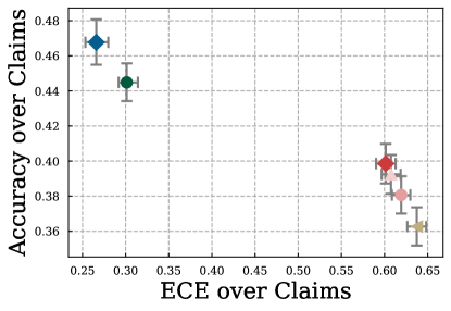
Figure 6: Accuracy-ECE Frontier for Person Biography Generation, simulated forecaster (upper left is better). Accuracy and ECE are computed at the claim level, using a finetuned retrieval model and API-based LLM for fact checking, following Min et al. (2023). LC RL significantly outperforms non-confidence methods in accuracy and ECE.

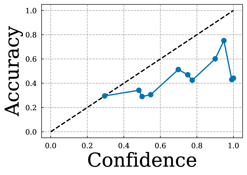
(a) LC SFT. ECE: $0.301$

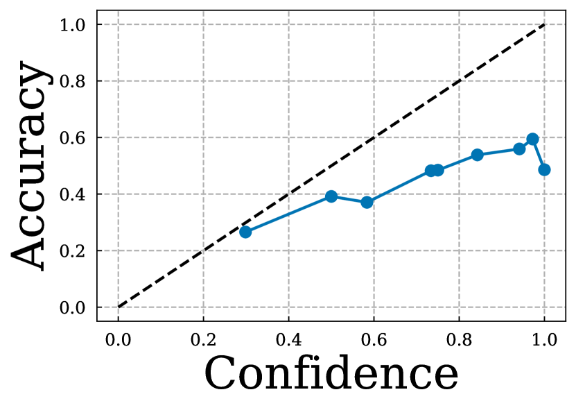
(b) LC RL. ECE: $0.266$

Figure 7: Person Biography Generation Reliability Diagrams for LC SFT (Left) and LC RL (Right); simulated forecaster. LC methods demonstrate non-trivial calibration in an entirely out-of-distribution task which requires calibrated statements of confidence throughout the paragraph.

4.3 Zero-Shot Generalization to a Biography Generation Task

The QA evaluation validated two of our three goals: (1) LC RL pareto-dominates baselines on the accuracy-ECE frontier. Its significant improvement over LC SFT validates the effectiveness of decision-based RL. (2) We demonstrated the computational efficiency of our training and evaluation framework, because LC RL is trained with cheap surrogates but performs well in evaluations with human forecasters, and our simulated forecasters have high agreement with human forecasters (see Appendix D.3 for full forecaster agreement statistics). Lastly, the QA evaluation partially validates (3) OOD generalization: LC RL performs well on the Jeopardy dataset with simulated forecasters.

To conclusively validate this final goal, we evaluate LC on a significant distribution shift in the task. Our models were trained to perform long-form generation about trivia-style questions, and we now test their ability to write factual biographies on people sampled from Wikipedia. Specifically, we source 500 people from the unlabeled split of FactScore Min et al. (2023) and use prompt “Write a paragraph bio about {person}” (cf. Fig. 5 for a qualitative example, and additional ones in Appendix A.8). We emphasize that our models were not trained on biography generation.

FactScore-based metric.

We also use a more fine-grained simulated evaluation than the QA tasks, testing the accuracy and calibration of generated biographies $z$ at the per-claim level. More specifically, we split generations into a list of claims, filter out subjective claims, and then pool all remaining claims across biographies to compute accuracy and ECE over all claims, following FactScore Min et al. (2023). Splitting and filtering steps are performed with Claude 2. We use an identical fact checking pipeline to Min et al. (2023) other than using Claude 2 instead of ChatGPT for fact-checking conditioned on retrieved context paragraphs from Wikipedia. In order to compute ECE, we need to assign confidence values to each atomic claim. For numerical uncertainties such as percentages, this is a simple extractive task which API-based LLMs perform well. For interpreting linguistic confidences into probabilities, we provide Claude 2 with a short list of mappings between linguistic phrases and consensus probabilities collected in a human study Wallsten (1990), and allow the LLM to generalize from this to assign probabilities for other linguistic phrases not present in the mapping. See Appendix D.2 for additional details.

LC generalizes to biography generation and claim-level evaluation.

Both LC methods demonstrate significant improvements in ECE and accuracy compared to non-confidence baselines, generalizing well to an entirely held-out task (Fig. 6). Because we here compute ECE at the per-claim level and the LC methods obtain reasonable ECE values and reliability diagrams (Fig. 7), we confirm that they incorporate calibrated statements of confidence throughout their long-form generations. Additionally, decision-based RL significantly improves both accuracy and ECE over LC SFT even under a significant task distribution shift, further validating our linguistic calibration objective.

Lastly, we note the surprising finding that LC SFT improves in accuracy compared to Factuality RL. We attribute this to the tendency of LC models to generate a higher proportion of less “precise” claims which are still objective and correct and therefore count towards the accuracy metric.

Altogether, our strong results in a challenging distribution shift setting validate our final goal.

5 Related Work

Calibration.

The calibration of probabilistic forecasts is an extensively studied topic Brier (1950), Murphy (1973), Dawid (1984), Zadrozny and Elkan (2001), Gneiting and Raftery (2007), Hebert-Johnson et al. (2018), Kull and Flach (2015). In particular, isotonic regression Niculescu-Mizil and Caruana (2005), Platt scaling Platt et al. (1999), temperature scaling Guo et al. (2017), and histogram binning Kumar et al. (2019) are effective approaches for improving the calibration of probability estimates. Other established methods improve calibration through ensembling (Lakshminarayanan et al., 2017) and Bayesian model averaging using an approximate posterior over model parameters Blundell et al. (2015), Gal and Ghahramani (2016), Band et al. (2021), Malinin et al. (2021), Nado et al. (2022), Tran et al. (2022).

Recent works also studied the probabilistic calibration of LMs, showing that LMs can be well-calibrated Kadavath et al. (2022). LMs that went through RL from human feedback (RLHF) tend to be ill-calibrated on multiple-choice questions OpenAI et al. (2023), but simple temperature scaling fixes the issue. Chain-of-thought prompting leads to ill-calibration Bai et al. (2022). The present focus is the linguistic calibration of LMs that produce long-form natural language, a setting to which established recalibration methods do not apply. This is because long-form generations may contain multiple claims, each of which has its confidence expressed in language.

Calibration and decision-making.

The particular decision-making framework we adopted was originally used to convey the confidence of individual predictions to decision-makers Zhao and Ermon (2021), and later used to draw an equivalence between different notions of calibration and optimal decision-making Zhao et al. (2021) (cf. §2.3 and Appendix B). In seminal work, Foster and Vohra (1999, 1998) showed that the existence of certain no regret schemes in an online decision-making setting imply the existence of calibrated probabilistic forecasts. More recently, Cresswell et al. (2024) explore using conformal prediction sets in classification tasks to improve human decision-making, but do not consider calibrating long-form LM generations.

LMs producing uncertainty.

The literature has studied methods to let LMs produce confidence scores or express uncertainty. Works have linguistically analyzed how LMs express uncertainty (Zhou et al., 2023), benchmarked the uncertainty quantification capabilities of LMs on multiple choice tasks (Ye et al., 2024), and studied how sampling variance could be used to estimate uncertainty (Malinin and Gales, 2021, Kuhn et al., 2023, Wang et al., 2022, Xiong et al., 2024).

Existing works on enabling LMs to directly express uncertainty have focused on short utterances (Mielke et al., 2022, Xiong et al., 2024), arithmetic problems (Lin et al., 2022), and question-answering (Jiang et al., 2021, Tian et al., 2023). All these prior works consider settings where the set of responses is a small closed set and the notion of calibration is well-defined. Other works finetune LMs to abstain Cheng et al. (2024) or to output templated uncertainty phrases Yang et al. (2023) on question-answering tasks. Lastly, concurrent work Huang et al. (2024) evaluates methods such as self-consistency Wang et al. (2022) and supervised finetuning in calibrating long-form generations. To the best of our knowledge, our method is the first to simultaneously provide calibrated text-based statements of confidence, which are important for interpretability to users Mielke et al. (2022), while working in the setting of long-form, multi-claim generations, which is how users interact with LLMs in practice. We overcome the challenge of defining calibration in this setting by drawing connections between decision-making and uncertainty quantification, enabling us to build a single end-to-end objective that can calibrate long-form generations.

Other LM finetuning works.

Improving the factuality of LMs is a complementary approach to calibration in mitigating LM hallucinations. Previous works have improved the factuality of LMs by finetuning on self-supervised or automated factuality scores Tian et al. (2024), Akyürek et al. (2024). A related line of work uses supervised finetuning and RL to improve the honesty of LLMs Askell et al. (2021), Ouyang et al. (2022), Park et al. (2023), Evans et al. (2021), Cui et al. (2023), hypothesizing that the pretraining objective alone is insufficient to encourage honest responses. Because improving factuality alone can improve calibration metrics such as ECE, we include a strong baseline finetuned with RL on ground-truth factuality labels and find that our approach to linguistic calibration significantly improves ECE beyond this baseline while matching or exceeding its accuracy.

6 Limitations, Future Work, and Conclusions

Limitations and Future Work.

Our linguistically calibrated LM generalizes well from surrogate to crowdworker forecasts. However, many of the confidence statements it emits are fairly unambiguous, e.g., percentages. Therefore, we believe investigating how LM interpretations of ambiguous linguistic confidence statements match up with human interpretations is important future work, and could enable training LMs with even better calibration of linguistic confidence statements that are tailored to user populations. Additionally, we use off-the-shelf question-answering datasets as a proxy for real-world decision-making tasks. Future work should consider curating a more representative dataset of decision-making tasks, to improve LC’s generalization to user decisions in-the-wild. Lastly, we work in a white-box setting where finetuning LMs is possible; our training framework could not be used to calibrate API-based LLMs that only provide access to completions.

Conclusions.

We defined linguistic calibration of long-form generations: calibrating the long-form generations of an LM in a way that leads to calibrated probabilistic forecasts by its downstream users. By constructing an objective in the space of these forecasts, we were able to apply the standard calibration machinery of proper scoring rules for end-to-end linguistic calibration. Instantiating this objective in a training framework and linguistically calibrating Llama 2 7B enables it to emit calibrated confidence statements, significantly improving the calibration of downstream human and simulated forecasts while matching or exceeding strong RL-tuned baselines in accuracy.

7 Acknowledgements

We thank Michael Y. Li, Yann Dubois, and members of the Tatsu Lab, Ma Lab, and Stanford Machine Learning Group for their helpful feedback. This work was supported by Open Philanthropy, IBM, NSF IIS 2211780, the Stanford HAI–Google Cloud Credits Program, and the Anthropic Researcher Access Program. NB acknowledges funding from an NSF Graduate Research Fellowship and a Quad Fellowship. XL acknowledges funding from a Stanford Graduate Fellowship and a Meta PhD Fellowship.

Linguistic Calibration of Language Models

Supplementary Material

Table of Contents

[sections] [sections]l1

Appendix A Additional Results

A.1 Additional Baselines

In addition to the baselines described in §4.1, we below provide full results including several other baselines. Throughout this paper’s experiments, we use GPT-4 version gpt-4-1106-preview and Claude 2 version claude-2.0. For question-answering dataset evaluations (TriviaQA and Jeopardy), all GPT-4 baselines are evaluated with 1000 evaluation samples (instead of approximately 11k) due to cost constraints. We refer the reader to the codebase for all prompts for all baselines and methods.

We include the following additional non-confidence baselines:

• Llama 2 Chat. We zero-shot prompt Llama 2 Chat to generate long-form responses to evaluation queries.

• GPT-4 0-Shot. We zero-shot prompt GPT-4 to generate long-form responses to evaluation queries.

• GPT-4 ICL 8-Shot. Analogous to the Llama 2 7B ICL baseline. We randomly sample 8 queries, generate long-form responses with GPT-4, manually fact-check those responses using Wikipedia, and use these fact-checked (query, response) pairs as ICL examples for GPT-4.

We also include the following additional confidence baselines:

• GPT-4 Just Ask for Uncertainty (JAFU) 0-Shot. We zero-shot prompt GPT-4 to generate long-form responses to evaluation queries, and include an instruction in the prompt directing GPT-4 to indicate any uncertainty in its claims using probabilities.

• GPT-4 Summary ICL 8-Shot. Analogous to the Llama 2 7B Summary ICL baseline. We sample 8 queries from the prompt development split $\{q^{(i)}\}_{i=1}^{8}$ (i.e., questions $x$ which have been converted to open-ended queries). For each query $q^{(i)}$, we generate 8 long-form responses from GPT-4: $\{z^{(i)}_{j}\}_{j=1}^{8}\sim\pi_{\text{GPT-4}}(z\mid q^{(i)})$. We then summarize these responses into a single consensus response: $s^{(i)}\sim\text{Summarize}(s\mid z^{(i)}_{1},\dots,z^{(i)}_{8})$. Finally, we use the queries and summaries as ICL examples $\{(q^{(i)},s^{(i)})\}_{i=1}^{8}$.

• Direct Summary Eval. For a given evaluation query $q$, we use the Llama 2 7B ICL baseline to generate 8 long-form responses $\{z_{i}\}_{i=1}^{8}$, and use Claude 2 to summarize these responses into a single consensus response: $s\sim\text{Summarize}(s\mid z_{1},\dots,z_{8})$. Then, we directly evaluate these summaries $s$. This is an oracle baseline because it requires sampling several long-form generations from the base LM at evaluation time, followed by summarization with an API-based LLM.

A.2 TriviaQA: Full Accuracy-ECE Frontier

A.3 TriviaQA: Additional Reliability Diagrams

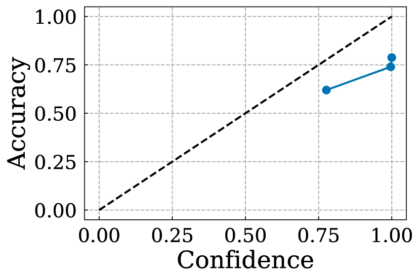
(a) GPT-4 JAFU 0-Shot. ECE: $0.212$

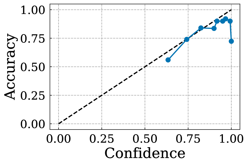
(b) GPT-4 Summary ICL 8-Shot. ECE: $0.119$

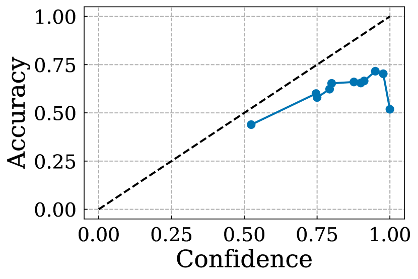
(c) Summary ICL 8-Shot. ECE: $0.257$

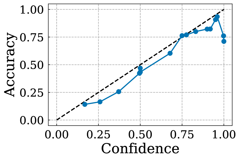
(d) Direct Summary Eval. ECE: $0.112$

Figure 9: TriviaQA Reliability Diagrams for additional baselines and oracle methods, simulated forecaster. Notably, Summary ICL works well for both Llama 2 7B (Summary ICL 8-Shot) and GPT-4. The oracle baseline of Direct Summary Eval has strong ECE.

A.4 Jeopardy: Full Accuracy-ECE Frontier

A.5 Jeopardy: All Reliability Diagrams

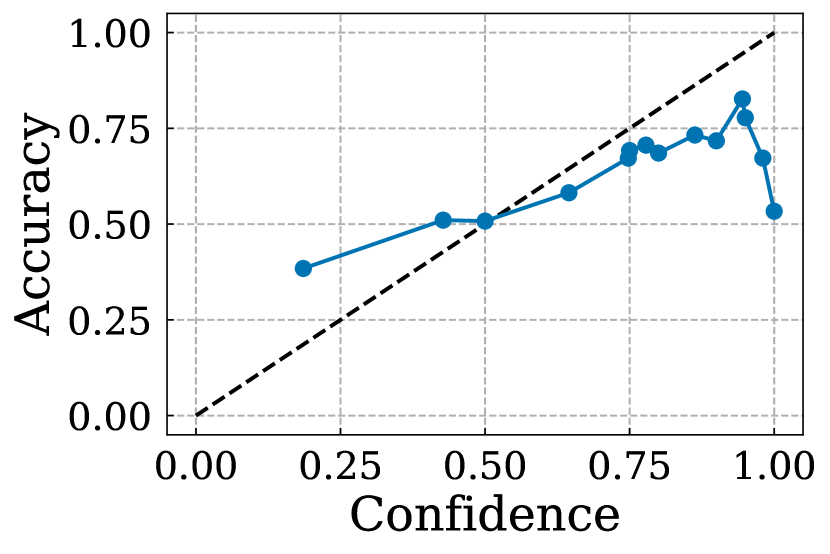
(a) LC SFT ($\pi_{\mathtt{SFT}})$. ECE: $0.162$

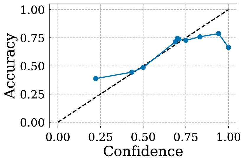
(b) LC RL ($\pi_{\mathtt{RL}})$. ECE: $0.088$

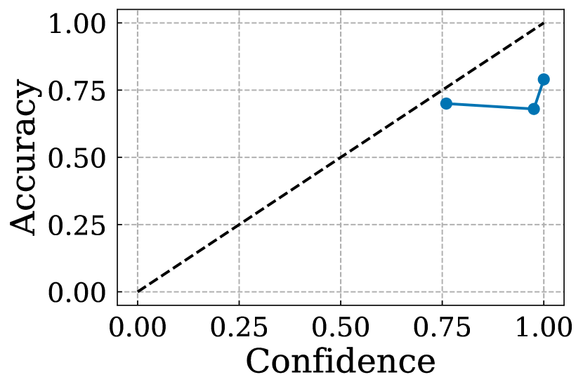
(c) GPT-4 JAFU 0-Shot. ECE: $0.207$

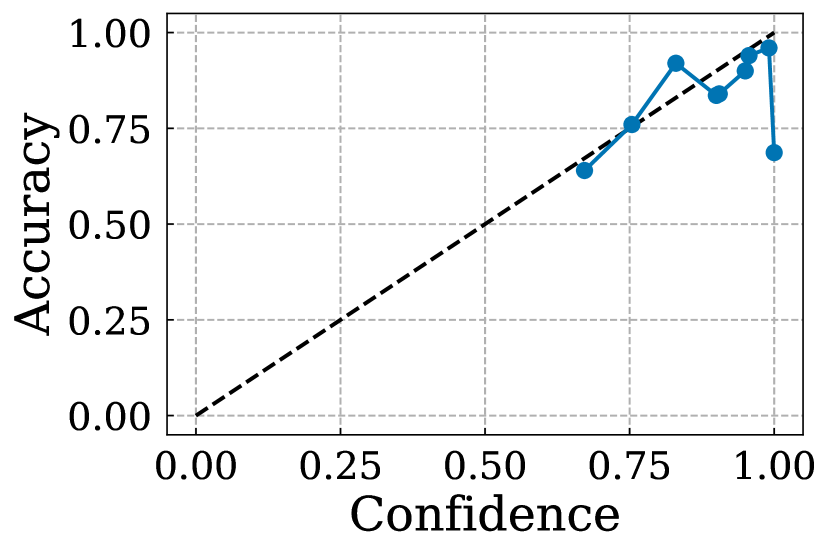
(d) GPT-4 Summary ICL 8-Shot. ECE: $0.130$

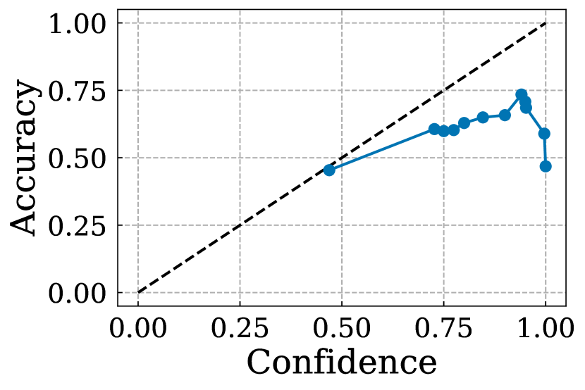
(e) Summary ICL 8-Shot. ECE: $0.254$

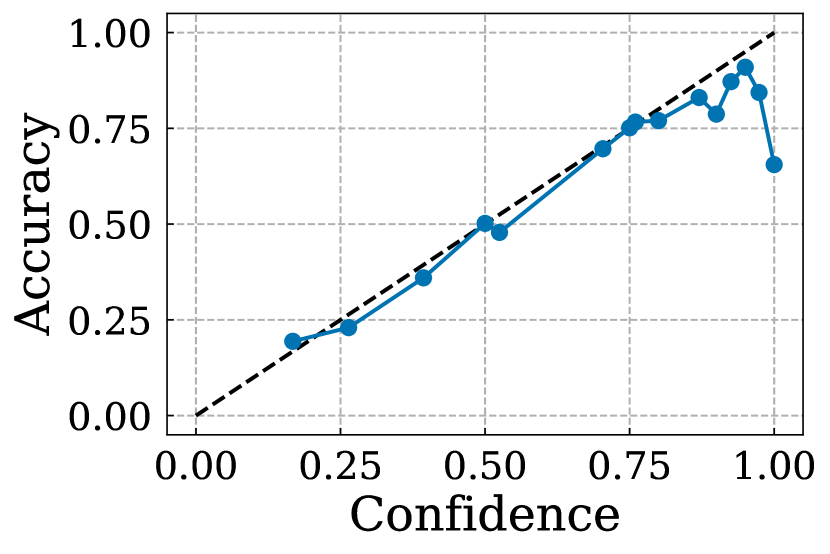
(f) Direct Summary Eval. ECE: $0.104$

Figure 11: Jeopardy Reliability Diagrams for all methods, simulated forecaster. LC RL has better ECE than all other methods while predicting a variety of confidence levels. Notably, Summary ICL works well for both Llama 2 7B (Summary ICL 8-Shot) and GPT-4. The oracle baseline of Direct Summary Eval has strong ECE.

A.6 Person Biography Generation Frontier

A.7 Tabular Results

Table 1: Question-Answering Results. Accuracy and expected calibration error (ECE) of Llama 2 7B and GPT-4–based methods on the in-distribution TriviaQA and out-of-distribution (OOD) Jeopardy question-answering datasets. We report results with simulated (sim.) and human forecasters for TriviaQA, and simulated forecaster for Jeopardy. “API-Based LLM Methods” are those that use either GPT-4 or Claude 2 at test time. 95% bootstrap CIs are reported as $(\text{lower},\text{upper})$.

	TriviaQA (sim. forecaster)		Jeopardy (OOD, sim. forecaster)		TriviaQA (human forecaster)
Method	Accuracy (%) $\uparrow$	ECE $\downarrow$	Accuracy (%) $\uparrow$	ECE $\downarrow$	Accuracy (%) $\uparrow$	ECE $\downarrow$
Llama 2 7B–Based Methods
Llama 2 Chat 7B	52.32 ${\scriptstyle(51.42,~{}53.27)}$	0.477 ${\scriptstyle(0.467,~{}0.486)}$	50.86 ${\scriptstyle(49.91,~{}51.82)}$	0.491 ${\scriptstyle(0.482,~{}0.501)}$	$-$	$-$
Claude Distill	60.89 ${\scriptstyle(59.98,~{}61.78)}$	0.391 ${\scriptstyle(0.382,~{}0.400)}$	60.54 ${\scriptstyle(59.64,~{}61.44)}$	0.395 ${\scriptstyle(0.386,~{}0.404)}$	$-$	$-$
ICL 8-Shot	61.91 ${\scriptstyle(61.02,~{}62.81)}$	0.381 ${\scriptstyle(0.372,~{}0.390)}$	61.63 ${\scriptstyle(60.69,~{}62.57)}$	0.384 ${\scriptstyle(0.374,~{}0.393)}$	$-$	$-$
Factuality SFT	61.17 ${\scriptstyle(60.26,~{}62.07)}$	0.388 ${\scriptstyle(0.379,~{}0.397)}$	62.13 ${\scriptstyle(61.21,~{}63.05)}$	0.379 ${\scriptstyle(0.370,~{}0.388)}$	$-$	$-$
Factuality RL	63.33 ${\scriptstyle(62.44,~{}64.21)}$	0.367 ${\scriptstyle(0.358,~{}0.376)}$	64.05 ${\scriptstyle(63.14,~{}64.97)}$	0.359 ${\scriptstyle(0.350,~{}0.369)}$	59.62 ${\scriptstyle(56.65,~{}62.60)}$	0.404 ${\scriptstyle(0.374,~{}0.434)}$
Summary ICL 8-Shot	61.36 ${\scriptstyle(60.47,~{}62.25)}$	0.257 ${\scriptstyle(0.248,~{}0.267)}$	60.90 ${\scriptstyle(59.98,~{}61.83)}$	0.254 ${\scriptstyle(0.245,~{}0.263)}$	$-$	$-$
LC SFT ($\pi_{\mathtt{SFT}})$	60.98 ${\scriptstyle(60.10,~{}61.88)}$	0.166 ${\scriptstyle(0.158,~{}0.176)}$	62.46 ${\scriptstyle(61.53,~{}63.36)}$	0.162 ${\scriptstyle(0.154,~{}0.172)}$	57.44 ${\scriptstyle(54.37,~{}60.52)}$	0.163 ${\scriptstyle(0.135,~{}0.192)}$
LC RL ($\pi_{\mathtt{LC}}$)	64.74 ${\scriptstyle(63.86,~{}65.63)}$	0.108 ${\scriptstyle(0.101,~{}0.117)}$	65.73 ${\scriptstyle(64.83,~{}66.61)}$	0.088 ${\scriptstyle(0.082,~{}0.098)}$	60.12 ${\scriptstyle(57.14,~{}63.19)}$	0.116 ${\scriptstyle(0.091,~{}0.145)}$
API-Based LLM Methods
GPT-4 0-Shot	78.00 ${\scriptstyle(75.30,~{}80.50)}$	0.220 ${\scriptstyle(0.195,~{}0.247)}$	77.60 ${\scriptstyle(75.00,~{}80.10)}$	0.224 ${\scriptstyle(0.199,~{}0.250)}$	$-$	$-$
GPT-4 ICL 8-Shot	80.80 ${\scriptstyle(78.40,~{}83.20)}$	0.192 ${\scriptstyle(0.168,~{}0.216)}$	82.30 ${\scriptstyle(80.00,~{}84.70)}$	0.177 ${\scriptstyle(0.153,~{}0.200)}$	$-$	$-$
GPT-4 JAFU 0-Shot	77.70 ${\scriptstyle(75.10,~{}80.20)}$	0.212 ${\scriptstyle(0.187,~{}0.238)}$	78.00 ${\scriptstyle(75.40,~{}80.50)}$	0.207 ${\scriptstyle(0.182,~{}0.234)}$	$-$	$-$
GPT-4 Summary ICL 8-Shot	80.40 ${\scriptstyle(77.90,~{}82.80)}$	0.119 ${\scriptstyle(0.104,~{}0.148)}$	80.30 ${\scriptstyle(77.80,~{}82.70)}$	0.130 ${\scriptstyle(0.111,~{}0.156)}$	$-$	$-$
Direct Summary Eval	63.67 ${\scriptstyle(62.78,~{}64.55)}$	0.112 ${\scriptstyle(0.105,~{}0.120)}$	64.50 ${\scriptstyle(63.59,~{}65.43)}$	0.104 ${\scriptstyle(0.098,~{}0.114)}$	$-$	$-$

Table 2: Person Biography Generation Results. Accuracy and expected calibration error (ECE) of Llama 2 7B and GPT-4–based methods on the Person Biography Generation dataset, using a FactScore-based automated metric Min et al. (2023). Metrics are computed over atomic claims pooled across all biography generations. 95% bootstrap CIs are reported as $(\text{lower},\text{upper})$.

Method	Accuracy (%) $\uparrow$	ECE $\downarrow$
Llama 2 7B–Based Methods
Llama 2 Chat 7B	36.27 ${\scriptstyle(35.18,~{}37.36)}$	0.637 ${\scriptstyle(0.626,~{}0.648)}$
Claude Distill	39.24 ${\scriptstyle(38.13,~{}40.34)}$	0.608 ${\scriptstyle(0.597,~{}0.619)}$
Factuality SFT	38.07 ${\scriptstyle(37.01,~{}39.13)}$	0.619 ${\scriptstyle(0.609,~{}0.630)}$
Factuality RL	39.86 ${\scriptstyle(38.72,~{}40.98)}$	0.601 ${\scriptstyle(0.590,~{}0.613)}$
LC SFT ($\pi_{\mathtt{SFT}})$	44.49 ${\scriptstyle(43.42,~{}45.57)}$	0.301 ${\scriptstyle(0.292,~{}0.314)}$
LC RL ($\pi_{\mathtt{LC}}$)	46.77 ${\scriptstyle(45.50,~{}48.08)}$	0.266 ${\scriptstyle(0.253,~{}0.280)}$
GPT-4–Based Methods
GPT-4 0-Shot	71.84 ${\scriptstyle(70.88,~{}72.81)}$	0.282 ${\scriptstyle(0.272,~{}0.291)}$
GPT-4 JAFU 0-Shot	75.95 ${\scriptstyle(74.93,~{}76.93)}$	0.210 ${\scriptstyle(0.200,~{}0.220)}$

A.8 Qualitative Examples

We randomly sample two examples from each evaluation dataset and compare Factuality RL with LC RL. We manually fact-check each generation using Wikipedia and other Google-accessible sources and highlight incorrect statements in red. Numerical and linguistic confidence statements are highlighted in blue.

Dataset: TriviaQA
Query $q$: Write a paragraph about the classic book in which a boy hides in a ship’s barrel of apples.
Ground-Truth Answer $y$: Treasure Island

Dataset: TriviaQA
Query $q$: Write a paragraph about the type of creature that a tanager is.
Ground-Truth Answer $y$: Bird

Dataset: Jeopardy
Query $q$: Write a paragraph about what Hiram Percy Maxim invented for guns, in addition to inventing the muffler for cars.
Ground-Truth Answer $y$: A silencer

Dataset: Jeopardy
Query $q$: Write a paragraph about the planet that a probe from the Galileo spacecraft plunged into the atmosphere of on December 7, 1995.
Ground-Truth Answer $y$: Jupiter

Dataset: Person Biography Generation
Query $q$: Write a paragraph bio about Griselda Blanco.

Dataset: Person Biography Generation
Query $q$: Write a paragraph bio about Uee.

Appendix B Benefits of Linguistic Calibration for Decision-making

In §2, we describe the connection between calibration and decision-making Zhao and Ermon (2021), Zhao et al. (2021) and how it motivates our objective for linguistic calibration: namely, that maximizing our objective implies zero expected regret for a downstream Bayes-optimal decision-maker. Here, we expand on this guarantee and provide additional ones using the results of Zhao et al. (2021), which apply even if we cannot perfectly maximize the linguistic calibration objective. In particular, we will see that forecasts fulfilling weaker notions of calibration still guarantee that decisions are optimal in a weaker sense.

For the remainder of the section, we assume that the linguistic calibration objective is optimized using samples from the real-world distribution of LM queries and related decision tasks $p(q,x,y)$. In practice, we found that using off-the-shelf question-answering datasets to generate a surrogate decision task distribution (cf. §3.1) robustly improves an LM’s ability to express confidence levels in text, including under distribution shift. Therefore, the generalization properties of LC may justify this assumption. Moreover, we believe an exciting avenue for future work is to curate a more representative decision task distribution (cf. §6).

B.1 Review of the LC Objective

Our decision-based RL algorithm optimizes a strictly proper scoring rule $R_{\texttt{LC}}$ of user forecasts with respect to an LM $\pi_{\text{RL}}$ producing long-form generations $z\sim\pi_{\text{RL}}(z\mid q)$ (restatement of Eq. 2 for convenience):

$$\max_{\pi_{\text{RL}}}\underset{(q,x,y)\sim p(q,x,y),~{}z\sim\pi_{\text{RL}}(z\mid q)}{\mathbb{E}}\left[R_{\texttt{LC}}\left(\widehat{p}(\cdot\mid x,z),y\right)\right].$$ (B.1)

Because $R_{\texttt{LC}}$ is strictly proper (cf. §2.3), if our training procedure maximizes Eq. B.1, then the user’s forecast exactly equals the ground-truth conditional distribution: $\widehat{p}(y\mid x,z)=p(y\mid x)$. Then, intuitively, making Bayes-optimal decisions according to the user forecast should be optimal in some sense. Zhao et al. (2021) make this notion of optimal decision-making concrete as decision calibration. We will provide the definition of decision calibration below, and then use it to precisely describe the guarantees that linguistic calibration provides for decision-making.

B.2 Decision Calibration

Setup and notation.

To define decision calibration, we first introduce some notation closely following Zhao et al. (2021), §2. Recall that in the user decision process, users receive a decision task question $x^{\prime}\in\mathcal{X}^{\prime}$, forecast a possible answer to the question with their forecaster function $\widehat{p}(y\mid\cdot):\mathcal{X}^{\prime}\rightarrow\Delta$, and finally choose from a set of available actions $\mathcal{A}$ based on their loss function $L:(\mathcal{A},\mathcal{Y})\rightarrow\mathbb{R}$ and their forecast $\widehat{p}(y\mid x^{\prime})\in\Delta$.

The process of choosing an action can be described by a decision rule which maps forecasts to actions $\delta:\Delta\rightarrow\mathcal{A}$, where ${{}_{\text{all}}}$ is the set of all decision rules. Additionally, define the set of all loss functions as $\mathcal{L}_{\text{all}}=\{L:(\mathcal{A},\mathcal{Y})\rightarrow\mathbb{R}\}$.

We are interested in Bayes decision rules, i.e., the set of rules that are optimal for some loss function. More specifically, consider some particular loss function $L\in\mathcal{L}_{\text{all}}$. Then its corresponding Bayes decision rule is

$$\delta_{L}(\widehat{p}(y\mid\cdot))=\operatorname*{arg\,min}_{a\in\mathcal{A}}\mathbb{E}_{\widehat{y}\sim\widehat{p}(y\mid\cdot)}[L(a,\widehat{y})].$$ (B.2)

For some subset $\mathcal{L}\subset\mathcal{L}_{\text{all}}$, we denote the corresponding Bayes decision rules as ${{}_{\mathcal{L}}}:=\{\delta_{L}\mid L\in\mathcal{L}\}.$

Decision calibration.

Zhao et al. (2021) defines decision calibration to formalize the following intuition: ideally, a decision-maker with loss function $L$ should be able to consider an arbitrary decision rule $\delta\in{{}_{\text{all}}}$ and compute the expected loss of using $\delta$ in decision-making, given a forecaster function $\widehat{p}(y\mid\cdot)$.

Definition B.1 (Decision Calibration, Definition 2 in Zhao et al. (2021)).

For any set of loss functions $\mathcal{L}\subset\mathcal{L}_{\text{all}}$, we say that a forecaster $\widehat{p}(y\mid\cdot)$ is $\mathcal{L}$-decision calibrated (with respect to the ground-truth conditional distribution $p(y\mid\cdot)$) if for each $L\in\mathcal{L}$ and $\delta\in{{}_{\mathcal{L}}}$,

$$\mathbb{E}_{x^{\prime}\sim p(x^{\prime})}\mathbb{E}_{\widehat{y}\sim\widehat{p}(y\mid x^{\prime})}\Big{[}L\big{(}\delta(\widehat{p}(y\mid x^{\prime})),\widehat{y}\big{)}\Big{]}=\mathbb{E}_{x^{\prime}\sim p(x^{\prime})}\mathbb{E}_{y\sim p(y\mid x^{\prime})}\Big{[}L\big{(}\delta(\widehat{p}(y\mid x^{\prime})),y\big{)}\Big{]}.$$ (B.3)

Following the analysis of Zhao et al. (2021) (§3.1), the left-hand side of Eq. B.3 simulates the loss of taking decisions according to the loss $L$ and rule $\delta$ using data drawn from the forecast $\widehat{y}\sim\widehat{p}(y\mid x^{\prime})$. This simulated loss can be computed by a user without observing any ground-truth outcome $y\sim p(y\mid\cdot)$. The right-hand side is the true loss for using decision rule $\delta$ with loss $L$. Therefore, decision calibration means that a forecaster function $\widehat{p}(y\mid\cdot)$ can be used to accurately estimate the expected loss of a decision rule under the true data distribution.

Decision calibration with LM assistance.

With a few particular choices, we can apply this general definition to the setting of LM-assisted decision-making. In our context, the relevant variables are the decision task question-answer pair $(x,y)$, the related query to the LM $q$, and the LM response $z$. These variables are distributed by the joint $p(q,x,y,z):=p(q,x,y)\pi_{\text{RL}}(z\mid q)$. Let $p(x,z):=\sum_{q^{\prime},y^{\prime}}p(q^{\prime},x,y^{\prime},z)$ be the marginal over questions and related LM responses. In the notation of Definition B.3, we define the input $x^{\prime}:=(x,z)$.

Lastly, we make the following technical conditional independence assumption, which we assume throughout the rest of the section.

Assumption B.2.

Under the ground-truth distribution, the answer $Y$ and the LM response $Z$ are conditionally independent given the question $X$: $p(Y\mid X,Z)=p(Y\mid X)$.

To be concrete, we reiterate decision calibration in our context, where users also condition their forecasts on LM outputs.

Definition B.3 (Decision Calibration with LM Assistance).

For any set of loss functions $\mathcal{L}\subset\mathcal{L}_{\text{all}}$, we say that an LM-assisted forecaster $\widehat{p}(y\mid\cdot):(\mathcal{X},\mathcal{Z})\rightarrow\Delta$ is $\mathcal{L}$-decision calibrated (with respect to the ground-truth conditional distribution $p(y\mid\cdot)$) if for each $L\in\mathcal{L}$ and $\delta\in{{}_{\mathcal{L}}}$,

$$\mathbb{E}_{(x,z)\sim p(x,z)}\mathbb{E}_{\widehat{y}\sim\widehat{p}(y\mid x,z)}\Big{[}L\big{(}\delta(\widehat{p}(y\mid x,z)),\widehat{y}\big{)}\Big{]}=\mathbb{E}_{(x,z)\sim p(x,z)}\mathbb{E}_{y\sim p(y\mid x)}\Big{[}L\big{(}\delta(\widehat{p}(y\mid x,z)),y\big{)}\Big{]}.$$

Zhao et al. (2021) proves that if a forecaster function $\widehat{p}(y\mid\cdot)$ is decision calibrated, it provides the downstream decision-maker with two key guarantees. First, a decision-maker with loss $L$ is assured that the Bayes decision rule $\delta_{L}$ outperforms alternative decision rules. Second, the decision-maker is able to accurately estimate the loss that they will incur by using the Bayes decision rule $\delta_{L}$, despite not having access to outcomes $y\sim p(y\mid\cdot)$. These guarantees are stated formally in the below proposition from Zhao et al. (2021) instantiated for our LM-assisted setting.

Proposition B.4 (instantiation of Proposition 1 in Zhao et al. (2021)).

If a forecaster $\widehat{p}(y\mid\cdot)$ is $\mathcal{L}$-decision calibrated, then it satisfies:

1. No regret: for each $\delta^{\prime}\in{{}_{\mathcal{L}}}$,

   $$\mathbb{E}_{(x,z)\sim p(x,z)}\mathbb{E}_{y\sim p(y\mid x)}\Big{[}L\big{(}\delta_{L}(\widehat{p}(y\mid x,z)),y\big{)}\Big{]}\leq\mathbb{E}_{(x,z)\sim p(x,z)}\mathbb{E}_{y\sim p(y\mid x)}\Big{[}L\big{(}\delta^{\prime}(\widehat{p}(y\mid x,z)),y\big{)}\Big{]}.$$

2. Accurate loss estimation:

   $$\mathbb{E}_{(x,z)\sim p(x,z)}\mathbb{E}_{\widehat{y}\sim\widehat{p}(y\mid x,z)}\Big{[}L\big{(}\delta_{L}(\widehat{p}(y\mid x,z)),\widehat{y}\big{)}\Big{]}=\mathbb{E}_{(x,z)\sim p(x,z)}\mathbb{E}_{y\sim p(y\mid x)}\Big{[}L\big{(}\delta_{L}(\widehat{p}(y\mid x,z)),y\big{)}\Big{]}.$$

To summarize, no regret means that the Bayes decision rule $\delta_{L}$ performs no worse than any other decision rule $\delta^{\prime}\in{{}_{\mathcal{L}}}$. Accurate loss estimation means that the decision-maker can determine before observing any ground-truth outcomes what their expected loss will be, allowing them to prepare for the future.

B.3 Linguistic Calibration and Optimal Decision-making

Now that we have defined decision calibration in our context, we can precisely describe the guarantees that linguistic calibration can provide for decision-making. We do so using a key result from Zhao et al. (2021) (Theorem 1): standard notions of calibration are equivalent to $\mathcal{L}$-decision calibration for particular choices of the loss family $\mathcal{L}$. We highlight two such notions of calibration here and direct the interested reader to Zhao et al. (2021) for others.

A distribution calibrated forecaster implies $\mathcal{L}_{\text{all}}$-decision calibration.

The strongest standard notion of calibration is distribution calibration Bröcker (2009). Intuitively, a forecaster $\widehat{p}(y\mid\cdot)$ is distribution calibrated if its forecast $p:=\widehat{p}(y\mid x^{\prime})\in\Delta$ is faithful to the predictive uncertainty Minderer et al. (2021). For example, among all inputs $x^{\prime}$ for which the forecasted probability of class $y^{\prime}$ is 0.4 (i.e., $p_{y^{\prime}}=0.4$), 40% of those inputs should have label $y^{\prime}$. Formally, for each $p\in\Delta$,

$$\Pr\left(Y=y^{\prime}\mathrel{\Big{|}}\widehat{p}(y\mid x^{\prime})=p\right)=p_{y^{\prime}}.$$

Zhao et al. (2021) (Theorem 1) proves that distribution calibration is equivalent to $\mathcal{L}_{\text{all}}$-decision calibration. Therefore, if we optimize the linguistic calibration objective $R_{\texttt{LC}}$ in Eq. B.1 and obtain a forecaster function $\widehat{p}(y\mid\cdot)$ that is distribution calibrated—for example, by maximizing $R_{\texttt{LC}}$—then the forecaster is $\mathcal{L}_{\text{all}}$-decision calibrated, and therefore a Bayes-optimal decision-maker is guaranteed to perform no worse than any decision rule $\delta^{\prime}\in{{}_{\text{all}}}$. Unsurprisingly, this is very difficult to achieve in practice. However, we will next show that even if linguistic calibration only manages to calibrate the forecaster in a weaker sense, we still have $\mathcal{L}$-decision calibration with respect to a smaller family of losses $\mathcal{L}$.

A confidence calibrated forecaster implies $\mathcal{L}_{\text{r}}$-decision calibration.

Likely the most common notion of calibration in the deep learning literature is confidence calibration. Confidence calibration is a relaxation of the distribution calibration condition, only requiring it to hold for the most likely label. Specifically, a forecaster $\widehat{p}(y\mid\cdot)$ is confidence calibrated Guo et al. (2017), Minderer et al. (2021) if among the examples with top forecasted probability equal to $\beta$, the accuracy over those examples is also $\beta$; i.e., for all $\beta\in[0,1]$,

$$\Pr\left(Y=\operatorname*{arg\,max}_{y}\widehat{p}(y\mid x^{\prime})\mathrel{\Big{|}}\max_{y}\widehat{p}(y\mid x^{\prime})=\beta\right)=\beta.$$

Zhao et al. (2021) (Theorem 1) demonstrates that confidence calibration is equivalent to $\mathcal{L}_{\text{r}}$-decision calibration, where

$$\mathcal{L}_{\text{r}}:=\Big{\{}L(a,y)=\mathbbm{1}[y\neq a\cap a\neq\perp]+\beta\cdot\mathbbm{1}[a=\perp]\mathrel{\big{|}}a\in\mathcal{Y}\cup\{\perp\},\forall\beta\in[0,1]\Big{\}}.$$ (B.4)

$\mathcal{L}_{\text{r}}$ is the class of loss functions for the refrained prediction task, where the decision-maker can either take an action corresponding to an answer $y\in\mathcal{Y}$ or report “I don’t know” with the action $\perp$. Then, the decision-maker incurs a loss of 0 for correctly predicting the ground-truth answer $y$, a loss of 1 for predicting an incorrect answer, or a loss of $\beta<1$ for reporting $\perp$.

Formal definition of linguistic calibration.

Linguistic calibration is a property of an LM generating responses $z$, and is defined with respect to a calibration metric $\phi$ and a given user. It means that the responses $z$ of the LM enable that user to make calibrated forecasts according to $\phi$. Formally:

Definition B.5 (Linguistic Calibration).

Consider an LM $\pi_{\text{RL}}$ producing long-form generations $z\sim\pi_{\text{RL}}(z\mid q)$, a calibration metric $\phi$ for a classifier (such as confidence calibration), and a user that is specified by their LM-assisted forecaster function $\widehat{p}(y\mid\cdot):(\mathcal{X},\mathcal{Z})\rightarrow\Delta$. Let $p(q,x,y,z):=p(q,x,y)\pi_{\text{RL}}(z\mid q)$ be the joint distribution over LM queries $q$, decision task pairs $(x,y)$, and LM generations $z$.

Then we say that $\pi_{\text{RL}}$ is $\phi$-linguistically calibrated with respect to $\widehat{p}(y\mid\cdot)$ if $\widehat{p}(y\mid\cdot)$ is $\phi$-calibrated over the marginal distribution of forecaster inputs and outputs $p(x,z,y):=\sum_{q^{\prime}}p(q^{\prime},x,y,z)$.

As a concrete example, let us consider linguistic calibration with respect to the confidence calibration metric $\phi_{\text{cc}}$. If $\pi_{\text{RL}}$ is $\phi_{\text{cc}}$-linguistically calibrated with respect to a forecaster $\widehat{p}(y\mid\cdot)$, then over the distribution $p(x,z,y)$, the forecaster $\widehat{p}(y\mid\cdot)$ is confidence calibrated, i.e., for all $\beta\in[0,1]$,

$$\Pr\left(Y=\operatorname*{arg\,max}_{y}\widehat{p}(y\mid x,z)\mathrel{\Big{|}}\max_{y}\widehat{p}(y\mid x,z)=\beta\right)=\beta.$$

Drawing the link through linguistic calibration, confidence calibration, and $\mathcal{L}_{\text{r}}$-decision calibration, we have the following proposition:

Proposition B.6 ($\phi_{\text{cc}}$-linguistic calibration enables Bayes-optimal decisions to outperform any $\delta^{\prime}\in{}_{\mathcal{L}_{\text{r}}}$.).

Suppose that

• An LM $\pi_{\text{RL}}$ is $\phi_{\text{cc}}$-linguistically calibrated with respect to a user with LM-assisted forecaster function $\widehat{p}(y\mid\cdot):(\mathcal{X},\mathcal{Z})\rightarrow\Delta$.

• The user’s loss function $L:(\mathcal{A},\mathcal{Y})\rightarrow\mathbb{R}$ is in the set of refrained prediction losses $\mathcal{L}_{\text{r}}$ (cf. Eq. B.4).

• The conditional independence assumption B.2 holds.

Define $\delta_{L}$ as the Bayes decision rule with respect to loss $L$ and ${}_{\mathcal{L}_{\text{r}}}$ as the set of all Bayes decision rules induced by $\mathcal{L}_{\text{r}}$. Then we have that $\forall\delta^{\prime}\in{}_{\mathcal{L}_{\text{r}}}$,

$$\mathbb{E}_{(x,z)\sim p(x,z)}\mathbb{E}_{y\sim p(y\mid x)}\Big{[}L\big{(}\delta_{L}(\widehat{p}(y\mid x,z)),y\big{)}\Big{]}\leq\mathbb{E}_{(x,z)\sim p(x,z)}\mathbb{E}_{y\sim p(y\mid x)}\Big{[}L\big{(}\delta^{\prime}(\widehat{p}(y\mid x,z)),y\big{)}\Big{]}.$$ (B.5)

Proof.

Recall that $p(x,z):=\sum_{q^{\prime},y^{\prime}}p(q^{\prime},x,y^{\prime},z)$ is the marginal over questions and related LM responses. Let $x^{\prime}:=(x,z)$ and $p(x^{\prime}):=p(x,z)$. Using the confidence calibration of the forecaster, apply Theorem 1 from Zhao et al. (2021) (equivalence of confidence calibration and $\mathcal{L}_{\text{r}}$-decision calibration) to observe that $\widehat{p}(y\mid\cdot)$ is $\mathcal{L}_{\text{r}}$-decision calibrated according to Definition B.3, Eq. B.3.

Now an application of Proposition 1 from Zhao et al. (2021) (in particular, the no regret guarantee of decision calibration) and the conditional independence statement $p(Y\mid X,Z)=p(Y\mid X)$ (Assumption B.2) gives the desired no regret condition (B.5). ∎

Because of the equivalence of confidence calibration and $\mathcal{L}_{\text{r}}$-decision calibration, if our optimization of $R_{\texttt{LC}}$ produces a confidence calibrated forecaster function $\widehat{p}(y\mid\cdot)$, we obtain $\mathcal{L}_{\text{r}}$-decision calibration and its corresponding guarantees for the decision-maker. Because confidence calibration is weaker than distribution calibration, this implies that the Bayes decision rule $\delta_{L}$ is guaranteed to outperform decision rules $\delta^{\prime}\in{}_{\mathcal{L}_{\text{r}}}$, where ${}_{\mathcal{L}_{\text{r}}}$ is a set of decision rules induced by $\mathcal{L}_{\text{r}}$ and is therefore a more restricted set than ${{}_{\text{all}}}$.

Summary: linguistic calibration provides optimal decision-making guarantees.

If we maximize the linguistic calibration objective, our forecasts are distribution calibrated and therefore we obtain $\mathcal{L}_{\text{all}}$-decision calibration, i.e., the Bayes optimal decision rule outperforms all other decision rules. Even if our optimization only achieves a weaker notion of calibration such as confidence calibration, we still obtain decision calibration over a more restricted class of loss functions. This fact also justifies our use of forecast ECE as an evaluation metric, because it estimates confidence calibration and can therefore be thought of as a proxy for the quality of downstream user decision-making. For further discussion, we direct the reader to Zhao et al. (2021) and Zhao and Ermon (2021).

Appendix C Training Framework

Linguistic calibration is a general-purpose definition that is agnostic to the particular design decisions we made in our proof-of-concept training framework. Nevertheless, this section details the design choices we made, including the regularized objective function we used to train with our neural net–based surrogate forecaster, and our implementation of PPO.

C.1 Regularized Linguistic Calibration Objective

Objective regularized to encourage normalized surrogate forecasts.

In our instantiation of linguistic calibration, we use a surrogate forecast $\widetilde{p}(y\mid x,z)$ which is not guaranteed to be normalized: we may have $\widetilde{p}(y\mid x,z)\in[0,1]^{K}\setminus\Delta$. We remedy this by adding a regularization term in the reward function which encourages $\widetilde{p}(y\mid x,z)$ to be normalized, restoring strict propriety (cf. §2.3) even with forecasts in $[0,1]^{K}$. We indeed find in practice that training with this objective results in normalized forecasts.

Our regularized reward function $R_{\texttt{LC}}:([0,1]^{K},\mathcal{Y})\rightarrow R$ is written as:

$$R_{\texttt{LC}}(\widetilde{p}(\cdot\mid x,z),y^{\prime})=\log\widetilde{p}(y^{\prime}\mid x,z)-\lambda\left|1-\sum_{y\in\mathcal{Y}}\widetilde{p}(y\mid x,z)\right|+C,$$ (C.6)

where $\lambda>0,C>0$ are hyperparameters. $C$ is a small positive constant which we find to reduce reward hacking during PPO.

Below, we prove that with $\lambda>1$, we indeed have a strictly proper objective.

C.2 Proof: Regularized Objective is Strictly Proper

Setup.

In decision-based RL, we wish to optimize an objective that encourages the surrogate forecast $\widetilde{p}(y\mid x,z)$ to exactly match the ground-truth distribution $p(y\mid x)$, which is supported over all possible answers in $\mathcal{Y},|\mathcal{Y}|=K$. Let $\Delta^{K-1}$ be the $(K-1)$-dimensional simplex. $\widetilde{p}(y\mid x,z)$ is not necessarily in $\Delta^{K-1}$ because it is obtained by several independent neural network predictions falling in the range $[0,1]$, i.e., $\widetilde{p}(y\mid x,z)\in[0,1]^{K}$. Therefore, in addition to a log loss term, we also add a regularizer which encourages $\widetilde{p}(y\mid x,z)$ to fall in the simplex, i.e., be normalized.

We would like our reward function to be strictly proper—its unique maximizer should be the ground-truth answer distribution. We will prove that our reward function is indeed strictly proper below. First, we define (strictly) proper scoring rules in our setting, which is slightly more general than the standard definition (e.g., in Gneiting and Raftery (2007)) in that the first argument need not be a probability distribution: it may fall in $[0,1]^{K}\setminus\Delta^{K-1}$. As shorthand throughout this proof, we will refer to the ground-truth answer distribution as $p^{*}:=p(y\mid x)$ and the forecast as $\widetilde{p}:=\widetilde{p}(y\mid x,z)$, because this proof is done pointwise for a given (question, LM generation) tuple $(x,z)$.

Definition C.1 (based on Gneiting and Raftery (2007)).

Let $\bar{\mathbb{R}}$ be the extended real line $[-\infty,\infty]$. A scoring rule $R:([0,1]^{K},\mathcal{Y})\rightarrow\bar{\mathbb{R}}$ is proper if

$$\mathbb{E}_{Y\sim p^{*}}[R(p^{*},Y)]\geq\mathbb{E}_{Y\sim p^{*}}[R(\widetilde{p},Y)],\quad\forall p^{*}\in\Delta^{(K-1)},\widetilde{p}\in[0,1]^{K}.$$ (C.7)

It is strictly proper if Eq. C.7 holds with equality if and only if $p^{*}=\widetilde{p}$.

Equivalently, we may express the strictly proper condition as

$$\mathbb{E}_{Y\sim p^{*}}[R(p^{*},Y)]>\mathbb{E}_{Y\sim p^{*}}[R(\widetilde{p},Y)],\quad\forall p^{*}\in\Delta^{(K-1)},\widetilde{p}\in[0,1]^{K},\widetilde{p}\neq p^{*}.$$ (C.8)

In proving that $R_{\texttt{LC}}$ is strictly proper, we will also make use of the following standard result:

Lemma 1 (e.g., Gneiting and Raftery (2007)).

The logarithmic scoring rule $R_{\log}:(\Delta^{(K-1)},\mathcal{Y})\rightarrow\{-\infty\}\cup\mathbb{R}$ is strictly proper.

Lastly, we will also use the log-sum inequality:

Lemma 2 (e.g., p. 29, Cover and Thomas (1991)).

Let $a_{1},\dots,a_{n}$ and $b_{1},\dots,b_{n}$ be nonnegative numbers. Denote $a:=\sum_{i=1}^{n}a_{i}$ and $b:=\sum_{i=1}^{n}b_{i}$. Then

$$\sum_{i=1}^{n}a_{i}\log\frac{a_{i}}{b_{i}}\geq a\log\frac{a}{b}.$$

We will now prove that our regularized training framework objective $R_{\texttt{LC}}$ is a strictly proper scoring rule using the condition for strict propriety in Eq. C.8.

Theorem C.2.

For any $C\in\mathbb{R}$ and with $\lambda>1$, the reward function $R_{\texttt{LC}}(\widetilde{p},y)$ from Eq. C.6 is strictly proper.

Proof.

Take an arbitrary $p^{*}\in\Delta^{(K-1)}$ and $\widetilde{p}\in[0,1]^{K}$ such that $\widetilde{p}\neq p^{*}$. We need to show that

$$\mathbb{E}_{Y\sim p^{*}}[R_{\texttt{LC}}(p^{*},Y)]-\mathbb{E}_{Y\sim p^{*}}[R_{\texttt{LC}}(\widetilde{p},Y)]>0.$$ (C.9)

All expectations for the rest of the proof are taken with respect to $p^{*}$, so we omit the subscript $Y\sim p^{*}$. We also identify the space of answers $\mathcal{Y}$ with the index set $[K]$, and therefore use notation $p_{y}$ to refer to the $y$-th index of the vector $p$. Lastly, we write $\sum_{y^{\prime}\in\mathcal{Y}}\widetilde{p}_{y^{\prime}}$ as $\bm{1}^{\top}\widetilde{p}$ for brevity.

Plugging in with our reward function, Inequality C.9 is equivalent to

$$\mathbb{E}\left[\log p^{*}_{Y}-\lambda|1-\bm{1}^{\top}p^{*}|+C\right]-\mathbb{E}\left[\log\widetilde{p}_{Y}-\lambda|1-\bm{1}^{\top}\widetilde{p}|+C\right]>0.$$

We can simplify the LHS by applying linearity of expectation and simplifying expectations of constants:

$$\text{LHS}=\mathbb{E}\left[\log p^{*}_{Y}\right]-\lambda|1-\bm{1}^{\top}p^{*}|-\mathbb{E}\left[\log\widetilde{p}_{Y}\right]+\lambda|1-\bm{1}^{\top}\widetilde{p}|.$$

Note that we assume $p^{*}\in\Delta^{(K-1)}$ so $\bm{1}^{\top}p^{*}=1$, and we can simplify further to

$$\text{LHS}=\mathbb{E}\left[\log p^{*}_{Y}\right]-\mathbb{E}\left[\log\widetilde{p}_{Y}\right]+\lambda|1-\bm{1}^{\top}\widetilde{p}|.$$ (C.10)

Now we proceed by cases on whether or not $\widetilde{p}\in\Delta^{(K-1)}$. Suppose that indeed $\widetilde{p}\in\Delta^{(K-1)}$. Then its normalization term $\lambda|1-\bm{1}^{\top}\widetilde{p}|$ is also 0, and therefore this inequality condition is precisely the strict propriety condition for the logarithmic scoring rule (including the assumption that both $p^{*}$ and $\widetilde{p}$ are in the simplex):

$$\mathbb{E}\left[\log p^{*}_{Y}\right]-\mathbb{E}\left[\log\widetilde{p}_{Y}\right]>0,$$

which is true according to Lemma 1, and therefore this case is done.

So now assume that $\widetilde{p}\in[0,1]^{K}\setminus\Delta^{(K-1)}$. This implies that its normalization term is greater than 0, i.e., $|1-\bm{1}^{\top}\widetilde{p}|>0$. In this case, we can prove using the properties of $\log$ and the log-sum inequality that the LHS expression in Eq. C.10 is greater than 0, in order to complete the proof.

First, we use the properties of $\log$ to rewrite the expectations in Eq. C.10 into the entropy of $p^{*}$ plus a relative entropy between $p^{*}$ and $\widetilde{p}$:

LHS $$=\mathbb{E}\left[\log p^{*}_{Y}\right]-\mathbb{E}\left[\log\widetilde{p}_{Y}\right]+\lambda|1-\bm{1}^{\top}\widetilde{p}|$$

$$=-\mathbb{H}[p^{*}]-\mathbb{E}\left[\log\widetilde{p}_{Y}\right]+\lambda|1-\bm{1}^{\top}\widetilde{p}| (\text{definition of entropy functional $\mathbb{H}[\cdot]$})$$

$$=-\mathbb{H}[p^{*}]+\mathbb{H}[p^{*}]+\sum_{y\in\mathcal{Y}}p^{*}_{y}\log\frac{p^{*}_{y}}{\widetilde{p}_{y}}+\lambda|1-\bm{1}^{\top}\widetilde{p}| (\text{decomposition of cross-entropy)}$$

$$=\sum_{y\in\mathcal{Y}}p^{*}_{y}\log\frac{p^{*}_{y}}{\widetilde{p}_{y}}+\lambda|1-\bm{1}^{\top}\widetilde{p}|,$$

where the penultimate step used the decomposition of cross-entropy $=$ entropy $+$ relative entropy.

We cannot immediately apply the information inequality to show that the relative entropy is nonnegative, because $\widetilde{p}$ is not a probability distribution (and therefore the KL Divergence and relative entropy are not the same; see, e.g., p. 90 in Boyd and Vandenberghe (2004)). However, we may use the log-sum inequality to finish the proof. Applying Lemma 2 using the fact that all elements of $p^{*}$ and $\widetilde{p}$ are nonnegative, we can lower bound the relative entropy term as

$$\sum_{y\in\mathcal{Y}}p^{*}_{y}\log\frac{p^{*}_{y}}{\widetilde{p}_{y}}\geq\bm{1}^{\top}p^{*}\log\frac{\bm{1}^{\top}p^{*}}{\bm{1}^{\top}\widetilde{p}}=\log\frac{1}{\bm{1}^{\top}\widetilde{p}}.$$

Altogether, substituting normalizer $\mathcal{Z}:=\bm{1}^{\top}\widetilde{p}$, we currently have a lower bound of the LHS in Eq. C.10 of

$$\text{LHS}\geq\log\frac{1}{\mathcal{Z}}+\lambda|1-\mathcal{Z}|.$$ (C.11)

Inspecting this function for $\lambda>1$, we can see that it is positive for all values of $\mathcal{Z}$ other than $\mathcal{Z}=1$. To be rigorous, we complete the proof with cases on the values of $\mathcal{Z}$. Because $\widetilde{p}\in[0,1]^{K}$, $\mathcal{Z}$ is nonnegative, and recall that we already covered the case when $\mathcal{Z}=\bm{1}^{\top}\widetilde{p}=1$ by reduction to strict propriety of the logarithmic scoring rule (Lemma 1).

When $\mathcal{Z}\in[0,1)$, we immediately see that $\log\frac{1}{\mathcal{Z}}>0$ and $\lambda|1-\mathcal{Z}|>0$ (since $\lambda>1$ by assumption), implying that the lower bound in Eq. C.11 is positive as we needed to show.

Lastly, suppose that $\mathcal{Z}\in[1,\infty)$. In that case, $\lambda|1-\mathcal{Z}|=\lambda(\mathcal{Z}-1)$. Now, note that the derivative of the lower bound in Eq. C.11 is positive for all $\mathcal{Z}\geq 1$ (recalling that $\lambda>1$):

$$\frac{d}{d\mathcal{Z}}\left[\log\frac{1}{\mathcal{Z}}+\lambda(\mathcal{Z}-1)\right]=-\frac{1}{\mathcal{Z}}+\lambda>-\frac{1}{\mathcal{Z}}+1,$$

e.g., at $\mathcal{Z}=1$, we have that the derivative is greater than $-\frac{1}{1}+1=0$. And further, at precisely $\mathcal{Z}=1$, the lower bound equals $\log\frac{1}{1}+\lambda|1-1|=0$. This proves that the lower bound is positive for all $\mathcal{Z}\in(1,\infty)$, which implies that the LHS is also positive for $\mathcal{Z}\in(1,\infty)$. We have covered all values of $\mathcal{Z}$, concluding that when $\lambda>1$, the reward function in Eq. C.6 is strictly proper. ∎

C.3 Additional Details on Training Framework

We provide additional details on the training framework below. For other details, we direct the reader to the codebase.

Training and Validation Splits.

Our training framework and all baselines use examples from the TriviaQA Joshi et al. (2017) unfiltered.nocontext subset on HuggingFace Datasets Lhoest et al. (2021). These examples are randomly assigned to the following splits:

• SFT ($10000$ examples): used for summary distillation and the other SFT baselines (Factuality SFT, Claude Distill).

• Prompt Validation ($1000$ examples): used for all ICL-based baselines and to construct ICL examples for simulated forecasting with an API-based LLM.

• Reward Model ($20000$ examples): used to train surrogate forecaster for LC, and binary reward model for Factuality RL baseline.

• PPO ($40000$ examples): used for PPO with LC RL and Factuality RL methods.

• PPO Validation ($1000$ examples): during PPO, we evaluate reward model rewards on this split and store checkpoints every 20 steps.

• Validation ($1000$ examples): used for tuning evaluation temperature and model selection for RL methods (described below).

Summary distillation details.

For each SFT dataset query $q$, we use the (non-confidence) ICL baseline to sample eight long-form generations $\{z_{i}\}_{i=1}^{8}\sim\pi_{\text{ICL}}(z\mid q)$ (temperature 0.7) that are then summarized using a Claude few-shot prompt $s\sim\text{Summarize}(s\mid z_{1},\dots,z_{8})$ (temperature 0.3). We use the dataset of $(q,s)$ pairs to finetune the base Llama 2 7B model, obtaining $\pi_{\text{SFT}}$. The same temperature settings are used for obtaining Summary ICL context examples, and for the Direct Summary Eval oracle baseline.

Surrogate and reward model details.

Following our evaluation protocol for user forecasts (§4.1), we specify prompt instructions so that LLM simulated forecasts $\widehat{p}_{\text{LLM}}(y\mid x,z)$ used in Algorithm 1 avoid the use of background knowledge. Dataset construction for the surrogate forecaster models ForecastProbs and ExtractAnswers is described in Algorithm 1.

For LC RL, we use the following training details:

• ForecastProbs: a Llama 2 7B–based model initialized with the LC SFT parameters and trained using a binary cross-entropy loss on prompts from the Reward Model split.

• ExtractAnswers: a RedPajama 3B–based model initialized from the pretrained model weights and trained with causal language modeling on targets formatted as a delimited list of possible answers, e.g., “Sushi; Sashimi; Nigiri”. We used a 3B model instead of Llama 2 7B due to computational constraints, i.e., to fit all standard PPO models such as the policy, reference policy, value model, and reward models into GPU memory on an 8x80GB A100 node.

For Factuality RL, we use the following training details:

• Reward Model: a Llama 2 7B–based model initialized with the Factuality SFT parameters and trained using binary cross-entropy loss on prompts from the Reward Model split, with binary correctness labels from Claude 2.0. In producing binary correctness labels for a given (question, ground-truth answer, generation) tuple $(x,y,z)$, Claude is given access to the ground-truth answer. Therefore, determining binary correctness is a simple extractive task that we find Claude performs with very high accuracy.

We tune all reward models over a wide range of learning rates; see codebase for details on hyperparameters.

PPO implementation and training.

We use a standard implementation of PPO from Dubois et al. (2023) and train with 8 80GB A100 GPUs using Flash Attention 2 Dao et al. (2022), Dao (2023) and PyTorch FSDP Zhao et al. (2023). For both PPO-based methods (LC RL and Factuality RL), we use default hyperparameters other than the following:

• We use a larger step batch size (512) with one optimization epoch per step for better training stability.

• We shorten query_len to 128 tokens, because our PPO inputs were essentially all under this length.

• We use a slightly lower temperature during the rollout phase ($0.7$ instead of $1.0$).

• We use the paged_adamw_8bit optimizer Dettmers et al. (2022) due to computational constraints. We also use this optimizer for SFT and reward model training for consistency, and find it had no negative impact on validation performance compared to AdamW Loshchilov and Hutter (2019).

• We train for $1500$ PPO steps.

We tune the KL penalty and learning rate of both PPO methods across a wide range, ultimately finding that kl_coef of $0.1$ and learning rate of 1e-5 works best for both methods.

For the LC RL objective, we find that $\lambda=5,C=5$ works well to enforce normalization of downstream forecasts and prevent reward hacking. In the log-loss term, we clip the probability of the ground-truth answer at $\epsilon=$1e-4 for numerical stability.

Model selection for RL methods.

We perform model selection for PPO-based methods (LC RL, Factuality RL) by taking the 5 PPO checkpoints with the highest reward model rewards on the PPO Validation split, evaluating them on the Validation split with the API-based LLM forecaster, and selecting the checkpoint with the best ECE.

Appendix D Evaluation Framework

Test Dataset Splits.

We use the following test dataset splits.

• TriviaQA Joshi et al. (2017) (11313 examples): take the validation split from the unfiltered.nocontext subset from HuggingFace Datasets Wolf et al. (2020), Lhoest et al. (2021).

• Jeopardy Kaggle (2020) (10638 examples): take a random sample of the train subset from HuggingFace Datasets. These questions are initially written in the indirect Jeopardy-style format (“For the last 8 years of his life, Galileo was under house arrest for espousing this man’s theory”), so we use Claude 2.0 to convert them into direct questions $x$.

• Person Biography Generation Min et al. (2023) (500 entities): use the unlabeled split of Wikipedia entities from the FactScore dataset.

As we do at training time (cf. §3.1), for TriviaQA and Jeopardy, we use an API-based LLM (Claude 2.0) to convert questions $x$ into open-ended queries $q$ that allow us to sample long-form generations $z\sim\pi(z\mid q)$ on the topic of the question $x$. For Person Biography Generation, we construct open-ended queries using the fixed template “Write a paragraph bio about {entity}.”.

D.1 Simulated Evaluation

Simulated forecaster.

Simulated forecasts $\widehat{p}(y\mid x,z)$ are a distribution over possible answers to the question $x$, based on long-form LM generations $z$. All simulated forecasts in this paper are formed using an API-based LLM—we use Claude 2.0 due to compute constraints, but other LLMs such as GPT-4 are well-capable of producing high-quality forecasts. These simulated forecasts are used in two parts of our training and evaluation frameworks:

• Training framework: simulated forecasts are used as ground-truth targets for training the surrogate forecaster (cf. Algorithm 1). Then the surrogate forecaster is used during PPO, enabling efficient training by avoiding calls to API-based LLMs.

• Evaluation framework: in our question-answering evaluations (TriviaQA and Jeopardy), we sample a held-out question-answer decision task pair $(x,y)\sim p(x,y)$, convert $x$ into open-ended query $q$, and evaluate the accuracy and ECE of the simulated forecast $\widehat{p}(y\mid x,z)$ for $z\sim\pi(z\mid q)$ sampled from a variety of LMs such as LC RL and Factuality RL.

In both cases, we obtain simulated forecasts by decomposing forecasting into two prompts, one for ExtractAnswers and one for ForecastProbs, following the description in §3. This is just one way of implementing a forecaster, and there are likely other reasonable ways to obtain high-quality probabilistic predictions.

In order to compute accuracy and ECE for the evaluation framework, we need to obtain the confidence and correctness of each forecast. We direct the reader to our codebase for all prompts.

Accuracy and ECE for confidence-based methods.

The confidence of a forecast is obtained by simply taking its argmax probability $\max_{y^{\prime}\in\mathcal{Y}}\widehat{p}(y^{\prime}\mid x,z)$. Recall that for question-answering evaluation datasets, we prompt an API-based LLM to perform the ForecastProbs operation. We find a zero-shot prompt is effective because confidence statements in $z$ associated with the question $x$ are usually numerical (and even when they are occasionally linguistic, Claude 2.0 produces reasonable confidence estimations). The correctness is obtained by determining whether the top answer in the forecast is correct, i.e., $\mathbbm{1}[y=\operatorname*{arg\,max}_{y^{\prime}\in\mathcal{Y}}\widehat{p}(y^{\prime}\mid x,z)]$. In practice, we perform this check by prompting Claude 2.0 with the question $x$, ground-truth answer choice $y$, and the argmax answer choice, and asking the LLM to decide whether the two answers are semantically equivalent, using few-shot ICL examples. We find this to be very reliable and it avoids the false negative issues that string match–based metrics encounter due to paraphrases.

Accuracy and ECE for non-confidence methods.

Our evaluation for non-confidence methods closely follows the pipeline for confidence-based methods. We extract answers using the ExtractAnswers prompt, which accounts for the possibility that models may provide multiple mutually exclusive answers to the question $x$. We select the “argmax” answer by taking the answer which appears first in the paragraph $z$. Because non-confidence methods are not prompted or trained to produce confidence statements, we fix their confidence values to 1. Then, we compute ECE for non-confidence methods in closed form as $(1-\text{Accuracy})$. This approach is validated by our human evaluations, in which the correlation between a fixed confidence value of 1 and the human-interpreted argmax probability of Factuality RL is 0.993, over 1000+ samples (cf. Table 5).

Temperature tuning.

We tuned the decoding temperature for generating paragraphs across the range $\{0.1,0.3,0.5,0.7\}$ for the core methods (LC RL, LC SFT, Factuality RL, Factuality SFT) on the TriviaQA Validation split with simulated forecaster evaluation. We found that temperature $0.3$ uniformly performed the best across methods. Therefore we defaulted to paragraph decoding temperature $0.3$ for evaluation throughout. We found that temperature $0.2$ consistently worked well for simulated forecaster operations ExtractAnswers, ForecastProbs, and for checking semantic equivalence.

Other evaluation details.

Because we prompt our LMs with open-ended queries ($q:=$ “Write a paragraph about $\{x\}$”) it is rarely possible that a paragraph $z$ will not provide information that answers question $x$. We account for this during evaluation by allowing the ExtractAnswers prompt to return an empty list if $z$ does not provide any plausible answers to the question. For any example with an empty extracted list, we consider the accuracy to be 0 and the confidence to be 1, which is the most conservative possible penalty for both accuracy and ECE. Because we significantly outperform baselines finetuned with RL for factuality, we account for the possibility of better responsiveness to the prompt (and therefore fewer empty ExtractAnswers lists) explaining our improvements.

D.2 FactScore-Based Evaluation Metric

We use an automated FactScore-based Min et al. (2023) metric using an API-based LLM (Claude 2.0 in our case) to test the accuracy and calibration of generated biographies $z$ at the per-claim level, probing for the quality of confidences throughout long-form generations. §4.3 describes this metric in detail. Prompts and code for this metric are available in our codebase.

Forecasting confidences.

As part of this metric, for confidence-based methods, we need to forecast probabilities which are used to compute ECE. As compared to the question-answering evaluations, this evaluation considers all claims in the generated paragraph and tends to have a higher proportion of claims with linguistic confidence statements. Therefore, we use the following procedure to assign probabilities to each claim. When a claim has a clear numerical uncertainty (e.g., a percentage) this is a simple extractive task which API-based LLMs perform well by default. For interpreting linguistic uncertainties, we provide the LLM with a mapping between linguistic phrases and probabilities collected in a linguistics human study Wallsten (1990), and allow it to generalize from this mapping to phrases that are not present in it (Table 3).

Linguistic Confidence Phrase	Probability
Almost Impossible	0.05
Doubtful	0.1
Improbable	0.1
Unlikely	0.15
Possible	0.3
Tossup	0.5
Good Chance	0.65
Likely	0.75
Probable	0.75
Almost Certain	0.95

Table 3: Ground-truth linguistic confidence mapping used in our FactScore probability interpretation prompt, from Wallsten (1990).

We believe that developing better strategies to interpret linguistic confidence statements in a manner tailored to a given user population is exciting future work (discussed in §6).

D.3 Human Evaluation

Task.

In order to compute our accuracy and ECE metrics using forecasts from human crowdworkers, we asked crowdworkers to provide the following for a given question, ground-truth answer, and long-form generation tuple $(x,y,z)$:

• Confidence: the argmax probability of their forecast distribution $\max_{y^{\prime}\in\mathcal{Y}}\widehat{p}(y^{\prime}\mid x,z)$.

• Correctness: a binary indicator of whether or not their top answer was correct, $\mathbbm{1}[y=\operatorname*{arg\,max}_{y^{\prime}\in\mathcal{Y}}\widehat{p}(y^{\prime}\mid x,z)]$.

We asked human crowdworkers to interpret the generated paragraphs literally, and provided a couple examples. These examples were intentionally selected to be unambiguous, i.e., numerical confidences, to ensure we were not biasing towards any particular manner of interpreting linguistic confidences.

Qualification.

We conducted two qualification rounds with our human annotators for the question-answering TriviaQA experiment. In the first round, we sent a single decision task example $(x,y)$ sampled from TriviaQA, along with 3 model outputs (from LC RL, LC SFT, and Factuality RL) to 117 workers, out of which 32 matched the expected output. This example was selected to be unambiguous. In the second round, we sent the 32 workers who passed the previous test a roughly hour-long test (examples also selected to be unambiguous; the student authors of this paper agreed on all confidence and correctness labels of the hour-long test). Among these annotators, we took the top 15 performers for the main annotation process.

Main annotation round.

During the main annotation process, we simply selected examples uniformly at random from the TriviaQA test set, including examples which were potentially ambiguous due to linguistic confidence statements. Overall, we collected annotations for 1008 examples (each with 3 model outputs) from human crowdworkers.

Quality assurance.

We compared crowdworker agreement with Claude 2.0 as a quality assurance measure. Five of the annotators had agreement rates which dropped significantly after the qualification round, from perfect performance on the hour-long test to less than 0.40 Cohen’s kappa agreement with Claude. Therefore, we discontinued working with these annotators and removed their labels.

Payment.

To determine payment, the authors of this paper timed our own completion time of the task, which was an average of approximately 1.3 minutes. Following best practices for crowdworker payment Whiting et al. (2019), Liang et al. (2023), we used a conservative estimate of annotation time of 3 minutes per task and set the per-task payment to $0.85 amounting to a compensation of $17 per hour, greater than the California minimum wage of $16 per hour.

Agreement statistics.

In Table 4 we report interannotator agreement (i.e., agreement between crowdworkers) computed over 5% of the collected samples, for each of the tested models.

Model	Correlation on Confidence	Cohen’s Kappa on Correctness
LC RL	0.886	0.850
LC SFT	0.719	0.842
Factuality RL	1.000	0.758

Table 4: Interannotator Agreement.

In Table 5, we report human agreement with Claude 2.0 over all examples.

Model	Correlation on Confidence	Cohen’s Kappa on Correctness
LC RL	0.626	0.739
LC SFT	0.618	0.748
Factuality RL	0.993	0.741

Table 5: Human-Claude 2.0 Agreement.

References

- Akyürek et al. (2024) Afra Feyza Akyürek, Ekin Akyürek, Leshem Choshen, Derry Wijaya, and Jacob Andreas. Deductive closure training of language models for coherence, accuracy, and updatability, 2024.
- Anthropic (2023) Anthropic. Model card and evaluations for claude models, 2023.
- Askell et al. (2021) Amanda Askell, Yuntao Bai, Anna Chen, Dawn Drain, Deep Ganguli, Tom Henighan, Andy Jones, Nicholas Joseph, Ben Mann, Nova DasSarma, Nelson Elhage, Zac Hatfield-Dodds, Danny Hernandez, Jackson Kernion, Kamal Ndousse, Catherine Olsson, Dario Amodei, Tom Brown, Jack Clark, Sam McCandlish, Chris Olah, and Jared Kaplan. A general language assistant as a laboratory for alignment, 2021.
- Bai et al. (2022) Yuntao Bai, Saurav Kadavath, Sandipan Kundu, Amanda Askell, Jackson Kernion, Andy Jones, Anna Chen, Anna Goldie, Azalia Mirhoseini, Cameron McKinnon, et al. Constitutional ai: Harmlessness from ai feedback. arXiv preprint arXiv:2212.08073, 2022.
- Band et al. (2021) Neil Band, Tim G. J. Rudner, Qixuan Feng, Angelos Filos, Zachary Nado, Michael W Dusenberry, Ghassen Jerfel, Dustin Tran, and Yarin Gal. Benchmarking bayesian deep learning on diabetic retinopathy detection tasks. In NeurIPS Datasets and Benchmarks Track, 2021.
- Blundell et al. (2015) Charles Blundell, Julien Cornebise, Koray Kavukcuoglu, and Daan Wierstra. Weight Uncertainty in Neural Networks. In Francis Bach and David Blei, editors, PMLR, volume 37 of Proceedings of Machine Learning Research, pages 1613–1622, Lille, France, 07–09 Jul 2015. PMLR.
- Boyd and Vandenberghe (2004) Stephen Boyd and Lieven Vandenberghe. Convex optimization. Cambridge University Press, 2004.
- Brier (1950) Glenn W. Brier. Verification of forecasts expressed in terms of probability. Monthly Weather Review, 78(1):1–3, 1950. doi: 10.1175/1520-0493(1950)078<0001:VOFEIT>2.0.CO;2. URL https://journals.ametsoc.org/view/journals/mwre/78/1/1520-0493_1950_078_0001_vofeit_2_0_co_2.xml.
- Bröcker (2009) Jochen Bröcker. Reliability, sufficiency, and the decomposition of proper scores. Quarterly Journal of the Royal Meteorological Society, 135(643):1512–1519, 2009. doi: https://doi.org/10.1002/qj.456. URL https://rmets.onlinelibrary.wiley.com/doi/abs/10.1002/qj.456.
- Cheng et al. (2024) Qinyuan Cheng, Tianxiang Sun, Xiangyang Liu, Wenwei Zhang, Zhangyue Yin, Shimin Li, Linyang Li, Zhengfu He, Kai Chen, and Xipeng Qiu. Can ai assistants know what they don’t know?, 2024.
- Cover and Thomas (1991) Thomas M. Cover and Joy A. Thomas. Elements of Information Theory. Wiley, New York, 1991.
- Cresswell et al. (2024) Jesse C. Cresswell, Yi Sui, Bhargava Kumar, and Noël Vouitsis. Conformal prediction sets improve human decision making, 2024.
- Cui et al. (2023) Ganqu Cui, Lifan Yuan, Ning Ding, Guanming Yao, Wei Zhu, Yuan Ni, Guotong Xie, Zhiyuan Liu, and Maosong Sun. Ultrafeedback: Boosting language models with high-quality feedback, 2023.
- Dahl et al. (2024) Matthew Dahl, Varun Magesh, Mirac Suzgun, and Daniel E. Ho. Large legal fictions: Profiling legal hallucinations in large language models, 2024.
- Dao (2023) Tri Dao. Flashattention-2: Faster attention with better parallelism and work partitioning, 2023.
- Dao et al. (2022) Tri Dao, Daniel Y. Fu, Stefano Ermon, Atri Rudra, and Christopher Ré. Flashattention: Fast and memory-efficient exact attention with io-awareness, 2022.
- Dawid (1984) A Philip Dawid. Present position and potential developments: Some personal views statistical theory the prequential approach. Journal of the Royal Statistical Society: Series A (General), 147(2):278–290, 1984.
- DeGroot and Fienberg (1983) Morris H. DeGroot and Stephen E. Fienberg. The comparison and evaluation of forecasters, 1983.
- Dettmers et al. (2022) Tim Dettmers, Mike Lewis, Sam Shleifer, and Luke Zettlemoyer. 8-bit optimizers via block-wise quantization, 2022.
- Dubois et al. (2023) Yann Dubois, Xuechen Li, Rohan Taori, Tianyi Zhang, Ishaan Gulrajani, Jimmy Ba, Carlos Guestrin, Percy Liang, and Tatsunori Hashimoto. Alpacafarm: A simulation framework for methods that learn from human feedback. In Thirty-seventh Conference on Neural Information Processing Systems, 2023. URL https://openreview.net/forum?id=4hturzLcKX.
- Evans et al. (2021) Owain Evans, Owen Cotton-Barratt, Lukas Finnveden, Adam Bales, Avital Balwit, Peter Wills, Luca Righetti, and William Saunders. Truthful ai: Developing and governing ai that does not lie, 2021.
- Foster and Vohra (1999) Dean P. Foster and Rakesh Vohra. Regret in the on-line decision problem. Games and Economic Behavior, 29(1):7–35, 1999. ISSN 0899-8256. doi: https://doi.org/10.1006/game.1999.0740. URL https://www.sciencedirect.com/science/article/pii/S0899825699907406.
- Foster and Vohra (1998) Dean P. Foster and Rakesh V. Vohra. Asymptotic calibration. Biometrika, 85(2):379–390, 1998. ISSN 00063444. URL http://www.jstor.org/stable/2337364.
- Gal and Ghahramani (2016) Yarin Gal and Zoubin Ghahramani. Dropout As a Bayesian Approximation: Representing Model Uncertainty in Deep Learning. In Proceedings of the 33rd International Conference on International Conference on Machine Learning - Volume 48, Icml 2016, pages 1050–1059, 2016.
- Gneiting and Raftery (2007) Tilmann Gneiting and Adrian E Raftery. Strictly proper scoring rules, prediction, and estimation. Journal of the American Statistical Association, 102(477):359–378, 2007. doi: 10.1198/016214506000001437. URL https://doi.org/10.1198/016214506000001437.
- Guo et al. (2017) Chuan Guo, Geoff Pleiss, Yu Sun, and Kilian Q. Weinberger. On calibration of modern neural networks. In Doina Precup and Yee Whye Teh, editors, Proceedings of the 34th International Conference on Machine Learning, volume 70 of Proceedings of Machine Learning Research, pages 1321–1330. PMLR, 06–11 Aug 2017. URL https://proceedings.mlr.press/v70/guo17a.html.
- Hebert-Johnson et al. (2018) Ursula Hebert-Johnson, Michael Kim, Omer Reingold, and Guy Rothblum. Multicalibration: Calibration for the (Computationally-identifiable) masses. In Jennifer Dy and Andreas Krause, editors, Proceedings of the 35th International Conference on Machine Learning, volume 80 of Proceedings of Machine Learning Research, pages 1939–1948. PMLR, 10–15 Jul 2018. URL https://proceedings.mlr.press/v80/hebert-johnson18a.html.
- Huang et al. (2023) Lei Huang, Weijiang Yu, Weitao Ma, Weihong Zhong, Zhangyin Feng, Haotian Wang, Qianglong Chen, Weihua Peng, Xiaocheng Feng, Bing Qin, and Ting Liu. A survey on hallucination in large language models: Principles, taxonomy, challenges, and open questions, 2023.
- Huang et al. (2024) Yukun Huang, Yixin Liu, Raghuveer Thirukovalluru, Arman Cohan, and Bhuwan Dhingra. Calibrating long-form generations from large language models, 2024.
- Ji et al. (2023) Ziwei Ji, Nayeon Lee, Rita Frieske, Tiezheng Yu, Dan Su, Yan Xu, Etsuko Ishii, Ye Jin Bang, Andrea Madotto, and Pascale Fung. Survey of hallucination in natural language generation. ACM Comput. Surv., 55(12), mar 2023. ISSN 0360-0300. doi: 10.1145/3571730. URL https://doi.org/10.1145/3571730.
- Jiang et al. (2021) Zhengbao Jiang, Jun Araki, Haibo Ding, and Graham Neubig. How Can We Know When Language Models Know? On the Calibration of Language Models for Question Answering. Transactions of the Association for Computational Linguistics, 9:962–977, 09 2021. ISSN 2307-387X. doi: 10.1162/tacl_a_00407. URL https://doi.org/10.1162/tacl_a_00407.
- Joshi et al. (2017) Mandar Joshi, Eunsol Choi, Daniel S. Weld, and Luke Zettlemoyer. Triviaqa: A large scale distantly supervised challenge dataset for reading comprehension. In Proceedings of the 55th Annual Meeting of the Association for Computational Linguistics, Vancouver, Canada, July 2017. Association for Computational Linguistics.
- Kadavath et al. (2022) Saurav Kadavath, Tom Conerly, Amanda Askell, Tom Henighan, Dawn Drain, Ethan Perez, Nicholas Schiefer, Zac Hatfield-Dodds, Nova DasSarma, Eli Tran-Johnson, Scott Johnston, Sheer El-Showk, Andy Jones, Nelson Elhage, Tristan Hume, Anna Chen, Yuntao Bai, Sam Bowman, Stanislav Fort, Deep Ganguli, Danny Hernandez, Josh Jacobson, Jackson Kernion, Shauna Kravec, Liane Lovitt, Kamal Ndousse, Catherine Olsson, Sam Ringer, Dario Amodei, Tom Brown, Jack Clark, Nicholas Joseph, Ben Mann, Sam McCandlish, Chris Olah, and Jared Kaplan. Language models (mostly) know what they know, 2022.
- Kaggle (2020) Kaggle. 200,000+ jeopardy! questions, 2020. URL https://www.kaggle.com/datasets/tunguz/200000-jeopardy-questions/data.
- Kuhn et al. (2023) Lorenz Kuhn, Yarin Gal, and Sebastian Farquhar. Semantic uncertainty: Linguistic invariances for uncertainty estimation in natural language generation, 2023.
- Kull and Flach (2015) Meelis Kull and Peter Flach. Novel decompositions of proper scoring rules for classification: Score adjustment as precursor to calibration. In Annalisa Appice, Pedro Pereira Rodrigues, Vítor Santos Costa, Carlos Soares, João Gama, and Alípio Jorge, editors, Machine Learning and Knowledge Discovery in Databases, pages 68–85, Cham, 2015. Springer International Publishing. ISBN 978-3-319-23528-8.
- Kumar et al. (2019) Ananya Kumar, Percy S Liang, and Tengyu Ma. Verified uncertainty calibration. Advances in Neural Information Processing Systems, 32, 2019.
- Lakshminarayanan et al. (2017) Balaji Lakshminarayanan, Alexander Pritzel, and Charles Blundell. Simple and Scalable Predictive Uncertainty Estimation using Deep Ensembles. In Isabelle Guyon, Ulrike von Luxburg, Samy Bengio, Hanna M. Wallach, Rob Fergus, S. V. N. Vishwanathan, and Roman Garnett, editors, Advances in Neural Information Processing Systems 30: Annual Conference on Neural Information Processing Systems 2017, December 4-9, 2017, Long Beach, CA, USA, pages 6402–6413, 2017.
- Lhoest et al. (2021) Quentin Lhoest, Albert Villanova del Moral, Yacine Jernite, Abhishek Thakur, Patrick von Platen, Suraj Patil, Julien Chaumond, Mariama Drame, Julien Plu, Lewis Tunstall, Joe Davison, Mario Šaško, Gunjan Chhablani, Bhavitvya Malik, Simon Brandeis, Teven Le Scao, Victor Sanh, Canwen Xu, Nicolas Patry, Angelina McMillan-Major, Philipp Schmid, Sylvain Gugger, Clément Delangue, Théo Matussière, Lysandre Debut, Stas Bekman, Pierric Cistac, Thibault Goehringer, Victor Mustar, François Lagunas, Alexander Rush, and Thomas Wolf. Datasets: A community library for natural language processing. In Proceedings of the 2021 Conference on Empirical Methods in Natural Language Processing: System Demonstrations, pages 175–184, Online and Punta Cana, Dominican Republic, November 2021. Association for Computational Linguistics. URL https://aclanthology.org/2021.emnlp-demo.21.
- Liang et al. (2023) Percy Liang, Rishi Bommasani, Tony Lee, Dimitris Tsipras, Dilara Soylu, Michihiro Yasunaga, Yian Zhang, Deepak Narayanan, Yuhuai Wu, Ananya Kumar, Benjamin Newman, Binhang Yuan, Bobby Yan, Ce Zhang, Christian Cosgrove, Christopher D. Manning, Christopher Ré, Diana Acosta-Navas, Drew A. Hudson, Eric Zelikman, Esin Durmus, Faisal Ladhak, Frieda Rong, Hongyu Ren, Huaxiu Yao, Jue Wang, Keshav Santhanam, Laurel Orr, Lucia Zheng, Mert Yuksekgonul, Mirac Suzgun, Nathan Kim, Neel Guha, Niladri Chatterji, Omar Khattab, Peter Henderson, Qian Huang, Ryan Chi, Sang Michael Xie, Shibani Santurkar, Surya Ganguli, Tatsunori Hashimoto, Thomas Icard, Tianyi Zhang, Vishrav Chaudhary, William Wang, Xuechen Li, Yifan Mai, Yuhui Zhang, and Yuta Koreeda. Holistic evaluation of language models, 2023.
- Lin et al. (2022) Stephanie Lin, Jacob Hilton, and Owain Evans. Teaching models to express their uncertainty in words, 2022.
- Loshchilov and Hutter (2019) Ilya Loshchilov and Frank Hutter. Decoupled weight decay regularization. In International Conference on Learning Representations, 2019.
- Malinin and Gales (2021) Andrey Malinin and Mark Gales. Uncertainty estimation in autoregressive structured prediction. In International Conference on Learning Representations, 2021. URL https://openreview.net/forum?id=jN5y-zb5Q7m.
- Malinin et al. (2021) Andrey Malinin, Neil Band, Yarin Gal, Mark Gales, Alexander Ganshin, German Chesnokov, Alexey Noskov, Andrey Ploskonosov, Liudmila Prokhorenkova, Ivan Provilkov, Vatsal Raina, Vyas Raina, Denis Roginskiy, Mariya Shmatova, Panagiotis Tigas, and Boris Yangel. Shifts: A Dataset of Real Distributional Shift Across Multiple Large-Scale Tasks. In Thirty-fifth Conference on Neural Information Processing Systems Datasets and Benchmarks Track, 2021.
- Mielke et al. (2022) Sabrina J. Mielke, Arthur Szlam, Emily Dinan, and Y-Lan Boureau. Reducing conversational agents’ overconfidence through linguistic calibration. Transactions of the Association for Computational Linguistics, 10:857–872, 2022. doi: 10.1162/tacl_a_00494. URL https://aclanthology.org/2022.tacl-1.50.
- Min et al. (2023) Sewon Min, Kalpesh Krishna, Xinxi Lyu, Mike Lewis, Wen-tau Yih, Pang Koh, Mohit Iyyer, Luke Zettlemoyer, and Hannaneh Hajishirzi. FActScore: Fine-grained atomic evaluation of factual precision in long form text generation. In Houda Bouamor, Juan Pino, and Kalika Bali, editors, Proceedings of the 2023 Conference on Empirical Methods in Natural Language Processing, pages 12076–12100, Singapore, December 2023. Association for Computational Linguistics. doi: 10.18653/v1/2023.emnlp-main.741. URL https://aclanthology.org/2023.emnlp-main.741.
- Minderer et al. (2021) Matthias Minderer, Josip Djolonga, Rob Romijnders, Frances Hubis, Xiaohua Zhai, Neil Houlsby, Dustin Tran, and Mario Lucic. Revisiting the calibration of modern neural networks. In M. Ranzato, A. Beygelzimer, Y. Dauphin, P.S. Liang, and J. Wortman Vaughan, editors, Advances in Neural Information Processing Systems, volume 34, pages 15682–15694. Curran Associates, Inc., 2021. URL https://proceedings.neurips.cc/paper_files/paper/2021/file/8420d359404024567b5aefda1231af24-Paper.pdf.
- Murphy (1973) Allan H Murphy. A new vector partition of the probability score. Journal of Applied Meteorology and Climatology, 12(4):595–600, 1973.
- Nado et al. (2022) Zachary Nado, Neil Band, Mark Collier, Josip Djolonga, Michael W. Dusenberry, Sebastian Farquhar, Qixuan Feng, Angelos Filos, Marton Havasi, Rodolphe Jenatton, Ghassen Jerfel, Jeremiah Liu, Zelda Mariet, Jeremy Nixon, Shreyas Padhy, Jie Ren, Tim G. J. Rudner, Faris Sbahi, Yeming Wen, Florian Wenzel, Kevin Murphy, D. Sculley, Balaji Lakshminarayanan, Jasper Snoek, Yarin Gal, and Dustin Tran. Uncertainty baselines: Benchmarks for uncertainty & robustness in deep learning, 2022.
- Niculescu-Mizil and Caruana (2005) Alexandru Niculescu-Mizil and Rich Caruana. Predicting good probabilities with supervised learning. In Proceedings of the 22nd International Conference on Machine Learning, ICML ’05, page 625–632, New York, NY, USA, 2005. Association for Computing Machinery. ISBN 1595931805. doi: 10.1145/1102351.1102430. URL https://doi.org/10.1145/1102351.1102430.
- OpenAI et al. (2023) OpenAI, Josh Achiam, Steven Adler, Sandhini Agarwal, Lama Ahmad, Ilge Akkaya, Florencia Leoni Aleman, Diogo Almeida, Janko Altenschmidt, Sam Altman, Shyamal Anadkat, Red Avila, Igor Babuschkin, Suchir Balaji, Valerie Balcom, Paul Baltescu, Haiming Bao, Mo Bavarian, Jeff Belgum, Irwan Bello, Jake Berdine, Gabriel Bernadett-Shapiro, Christopher Berner, Lenny Bogdonoff, Oleg Boiko, Madelaine Boyd, Anna-Luisa Brakman, Greg Brockman, Tim Brooks, Miles Brundage, Kevin Button, Trevor Cai, Rosie Campbell, Andrew Cann, Brittany Carey, Chelsea Carlson, Rory Carmichael, Brooke Chan, Che Chang, Fotis Chantzis, Derek Chen, Sully Chen, Ruby Chen, Jason Chen, Mark Chen, Ben Chess, Chester Cho, Casey Chu, Hyung Won Chung, Dave Cummings, Jeremiah Currier, Yunxing Dai, Cory Decareaux, Thomas Degry, Noah Deutsch, Damien Deville, Arka Dhar, David Dohan, Steve Dowling, Sheila Dunning, Adrien Ecoffet, Atty Eleti, Tyna Eloundou, David Farhi, Liam Fedus, Niko Felix, Simón Posada Fishman, Juston Forte, Isabella Fulford, Leo Gao, Elie Georges, Christian Gibson, Vik Goel, Tarun Gogineni, Gabriel Goh, Rapha Gontijo-Lopes, Jonathan Gordon, Morgan Grafstein, Scott Gray, Ryan Greene, Joshua Gross, Shixiang Shane Gu, Yufei Guo, Chris Hallacy, Jesse Han, Jeff Harris, Yuchen He, Mike Heaton, Johannes Heidecke, Chris Hesse, Alan Hickey, Wade Hickey, Peter Hoeschele, Brandon Houghton, Kenny Hsu, Shengli Hu, Xin Hu, Joost Huizinga, Shantanu Jain, Shawn Jain, Joanne Jang, Angela Jiang, Roger Jiang, Haozhun Jin, Denny Jin, Shino Jomoto, Billie Jonn, Heewoo Jun, Tomer Kaftan, Łukasz Kaiser, Ali Kamali, Ingmar Kanitscheider, Nitish Shirish Keskar, Tabarak Khan, Logan Kilpatrick, Jong Wook Kim, Christina Kim, Yongjik Kim, Hendrik Kirchner, Jamie Kiros, Matt Knight, Daniel Kokotajlo, Łukasz Kondraciuk, Andrew Kondrich, Aris Konstantinidis, Kyle Kosic, Gretchen Krueger, Vishal Kuo, Michael Lampe, Ikai Lan, Teddy Lee, Jan Leike, Jade Leung, Daniel Levy, Chak Ming Li, Rachel Lim, Molly Lin, Stephanie Lin, Mateusz Litwin, Theresa Lopez, Ryan Lowe, Patricia Lue, Anna Makanju, Kim Malfacini, Sam Manning, Todor Markov, Yaniv Markovski, Bianca Martin, Katie Mayer, Andrew Mayne, Bob McGrew, Scott Mayer McKinney, Christine McLeavey, Paul McMillan, Jake McNeil, David Medina, Aalok Mehta, Jacob Menick, Luke Metz, Andrey Mishchenko, Pamela Mishkin, Vinnie Monaco, Evan Morikawa, Daniel Mossing, Tong Mu, Mira Murati, Oleg Murk, David Mély, Ashvin Nair, Reiichiro Nakano, Rajeev Nayak, Arvind Neelakantan, Richard Ngo, Hyeonwoo Noh, Long Ouyang, Cullen O’Keefe, Jakub Pachocki, Alex Paino, Joe Palermo, Ashley Pantuliano, Giambattista Parascandolo, Joel Parish, Emy Parparita, Alex Passos, Mikhail Pavlov, Andrew Peng, Adam Perelman, Filipe de Avila Belbute Peres, Michael Petrov, Henrique Ponde de Oliveira Pinto, Michael, Pokorny, Michelle Pokrass, Vitchyr Pong, Tolly Powell, Alethea Power, Boris Power, Elizabeth Proehl, Raul Puri, Alec Radford, Jack Rae, Aditya Ramesh, Cameron Raymond, Francis Real, Kendra Rimbach, Carl Ross, Bob Rotsted, Henri Roussez, Nick Ryder, Mario Saltarelli, Ted Sanders, Shibani Santurkar, Girish Sastry, Heather Schmidt, David Schnurr, John Schulman, Daniel Selsam, Kyla Sheppard, Toki Sherbakov, Jessica Shieh, Sarah Shoker, Pranav Shyam, Szymon Sidor, Eric Sigler, Maddie Simens, Jordan Sitkin, Katarina Slama, Ian Sohl, Benjamin Sokolowsky, Yang Song, Natalie Staudacher, Felipe Petroski Such, Natalie Summers, Ilya Sutskever, Jie Tang, Nikolas Tezak, Madeleine Thompson, Phil Tillet, Amin Tootoonchian, Elizabeth Tseng, Preston Tuggle, Nick Turley, Jerry Tworek, Juan Felipe Cerón Uribe, Andrea Vallone, Arun Vijayvergiya, Chelsea Voss, Carroll Wainwright, Justin Jay Wang, Alvin Wang, Ben Wang, Jonathan Ward, Jason Wei, CJ Weinmann, Akila Welihinda, Peter Welinder, Jiayi Weng, Lilian Weng, Matt Wiethoff, Dave Willner, Clemens Winter, Samuel Wolrich, Hannah Wong, Lauren Workman, Sherwin Wu, Jeff Wu, Michael Wu, Kai Xiao, Tao Xu, Sarah Yoo, Kevin Yu, Qiming Yuan, Wojciech Zaremba, Rowan Zellers, Chong Zhang, Marvin Zhang, Shengjia Zhao, Tianhao Zheng, Juntang Zhuang, William Zhuk, and Barret Zoph. Gpt-4 technical report, 2023.
- Ouyang et al. (2022) Long Ouyang, Jeff Wu, Xu Jiang, Diogo Almeida, Carroll L. Wainwright, Pamela Mishkin, Chong Zhang, Sandhini Agarwal, Katarina Slama, Alex Ray, John Schulman, Jacob Hilton, Fraser Kelton, Luke Miller, Maddie Simens, Amanda Askell, Peter Welinder, Paul Christiano, Jan Leike, and Ryan Lowe. Training language models to follow instructions with human feedback, 2022. URL https://arxiv.org/abs/2203.02155.
- Park et al. (2023) Peter S. Park, Simon Goldstein, Aidan O’Gara, Michael Chen, and Dan Hendrycks. Ai deception: A survey of examples, risks, and potential solutions, 2023.
- Platt et al. (1999) John Platt et al. Probabilistic outputs for support vector machines and comparisons to regularized likelihood methods. Advances in large margin classifiers, 10(3):61–74, 1999.
- Thirunavukarasu et al. (2023) Arun James Thirunavukarasu, Darren Shu Jeng Ting, Kabilan Elangovan, Laura Gutierrez, Ting Fang Tan, and Daniel Shu Wei Ting. Large language models in medicine. Nature Medicine, 29(8):1930–1940, Aug 2023. ISSN 1546-170X. doi: 10.1038/s41591-023-02448-8. URL https://doi.org/10.1038/s41591-023-02448-8.
- Tian et al. (2023) Katherine Tian, Eric Mitchell, Allan Zhou, Archit Sharma, Rafael Rafailov, Huaxiu Yao, Chelsea Finn, and Christopher Manning. Just ask for calibration: Strategies for eliciting calibrated confidence scores from language models fine-tuned with human feedback. In Houda Bouamor, Juan Pino, and Kalika Bali, editors, Proceedings of the 2023 Conference on Empirical Methods in Natural Language Processing, pages 5433–5442, Singapore, December 2023. Association for Computational Linguistics. doi: 10.18653/v1/2023.emnlp-main.330. URL https://aclanthology.org/2023.emnlp-main.330.
- Tian et al. (2024) Katherine Tian, Eric Mitchell, Huaxiu Yao, Christopher D Manning, and Chelsea Finn. Fine-tuning language models for factuality. In The Twelfth International Conference on Learning Representations, 2024. URL https://openreview.net/forum?id=WPZ2yPag4K.
- together.ai (2023) together.ai. Releasing 3b and 7b redpajama-incite family of models including base, instruction-tuned & chat models, 2023. URL https://www.together.ai/blog/redpajama-models-v1.
- Tran et al. (2022) Dustin Tran, Andreas Kirsch, Balaji Lakshminarayanan, Huiyi Hu, Du Phan, D. Sculley, Jasper Snoek, Jeremiah Zhe Liu, Jie Ren, Joost van Amersfoort, Kehang Han, E. Kelly Buchanan, Kevin Patrick Murphy, Mark Collier, Michael W Dusenberry, Neil Band, Nithum Thain, Rodolphe Jenatton, Tim G. J. Rudner, Yarin Gal, Zachary Nado, Zelda E Mariet, Zi Wang, and Zoubin Ghahramani. Plex: Towards reliability using pretrained large model extensions. In ICML 2022 Workshop on Pre-training, 2022.
- Wallsten (1990) Thomas Wallsten. Measuring Vague Uncertainties and Understanding Their Use in Decision Making, pages 377–398. Measuring Vague Uncertainties and Understanding Their Use in Decision Making, 01 1990. ISBN 978-90-481-5785-3. doi: 10.1007/978-94-015-7873-8_15.
- Wang et al. (2022) Xuezhi Wang, Jason Wei, Dale Schuurmans, Quoc Le, Ed Chi, Sharan Narang, Aakanksha Chowdhery, and Denny Zhou. Self-consistency improves chain of thought reasoning in language models, 2022. URL https://arxiv.org/abs/2203.11171.
- Wang et al. (2023) Xuezhi Wang, Jason Wei, Dale Schuurmans, Quoc V Le, Ed H. Chi, Sharan Narang, Aakanksha Chowdhery, and Denny Zhou. Self-consistency improves chain of thought reasoning in language models. In The Eleventh International Conference on Learning Representations, 2023. URL https://openreview.net/forum?id=1PL1NIMMrw.
- Whiting et al. (2019) Mark E. Whiting, Grant Hugh, and Michael S. Bernstein. Fair work: Crowd work minimum wage with one line of code. Proceedings of the AAAI Conference on Human Computation and Crowdsourcing, 7(1):197–206, Oct. 2019. doi: 10.1609/hcomp.v7i1.5283. URL https://ojs.aaai.org/index.php/HCOMP/article/view/5283.
- Wolf et al. (2020) Thomas Wolf, Lysandre Debut, Victor Sanh, Julien Chaumond, Clement Delangue, Anthony Moi, Pierric Cistac, Tim Rault, Rémi Louf, Morgan Funtowicz, Joe Davison, Sam Shleifer, Patrick von Platen, Clara Ma, Yacine Jernite, Julien Plu, Canwen Xu, Teven Le Scao, Sylvain Gugger, Mariama Drame, Quentin Lhoest, and Alexander M. Rush. Transformers: State-of-the-art natural language processing. In Proceedings of the 2020 Conference on Empirical Methods in Natural Language Processing: System Demonstrations, pages 38–45, Online, October 2020. Association for Computational Linguistics. URL https://www.aclweb.org/anthology/2020.emnlp-demos.6.
- Xiong et al. (2024) Miao Xiong, Zhiyuan Hu, Xinyang Lu, YIFEI LI, Jie Fu, Junxian He, and Bryan Hooi. Can LLMs express their uncertainty? an empirical evaluation of confidence elicitation in LLMs. In The Twelfth International Conference on Learning Representations, 2024. URL https://openreview.net/forum?id=gjeQKFxFpZ.
- Yang et al. (2023) Yuqing Yang, Ethan Chern, Xipeng Qiu, Graham Neubig, and Pengfei Liu. Alignment for honesty, 2023.
- Ye et al. (2024) Fanghua Ye, Mingming Yang, Jianhui Pang, Longyue Wang, Derek F. Wong, Emine Yilmaz, Shuming Shi, and Zhaopeng Tu. Benchmarking llms via uncertainty quantification, 2024.
- Zadrozny and Elkan (2001) Bianca Zadrozny and Charles Elkan. Obtaining calibrated probability estimates from decision trees and naive bayesian classifiers. In Icml, volume 1, pages 609–616, 2001.
- Zhao and Ermon (2021) Shengjia Zhao and Stefano Ermon. Right decisions from wrong predictions: A mechanism design alternative to individual calibration. In Arindam Banerjee and Kenji Fukumizu, editors, Proceedings of The 24th International Conference on Artificial Intelligence and Statistics, volume 130 of Proceedings of Machine Learning Research, pages 2683–2691. PMLR, 13–15 Apr 2021. URL https://proceedings.mlr.press/v130/zhao21a.html.
- Zhao et al. (2021) Shengjia Zhao, Michael Kim, Roshni Sahoo, Tengyu Ma, and Stefano Ermon. Calibrating predictions to decisions: A novel approach to multi-class calibration. In M. Ranzato, A. Beygelzimer, Y. Dauphin, P.S. Liang, and J. Wortman Vaughan, editors, Advances in Neural Information Processing Systems, volume 34, pages 22313–22324. Curran Associates, Inc., 2021. URL https://proceedings.neurips.cc/paper_files/paper/2021/file/bbc92a647199b832ec90d7cf57074e9e-Paper.pdf.
- Zhao et al. (2023) Yanli Zhao, Andrew Gu, Rohan Varma, Liang Luo, Chien-Chin Huang, Min Xu, Less Wright, Hamid Shojanazeri, Myle Ott, Sam Shleifer, Alban Desmaison, Can Balioglu, Pritam Damania, Bernard Nguyen, Geeta Chauhan, Yuchen Hao, Ajit Mathews, and Shen Li. Pytorch fsdp: Experiences on scaling fully sharded data parallel, 2023.
- Zhou et al. (2023) Kaitlyn Zhou, Dan Jurafsky, and Tatsunori Hashimoto. Navigating the grey area: How expressions of uncertainty and overconfidence affect language models. In Houda Bouamor, Juan Pino, and Kalika Bali, editors, Proceedings of the 2023 Conference on Empirical Methods in Natural Language Processing, pages 5506–5524, Singapore, December 2023. Association for Computational Linguistics. doi: 10.18653/v1/2023.emnlp-main.335. URL https://aclanthology.org/2023.emnlp-main.335.