Addressing Both Statistical and Causal Gender Fairness in NLP Models

Abstract

Statistical fairness stipulates equivalent outcomes for every protected group, whereas causal fairness prescribes that a model makes the same prediction for an individual regardless of their protected characteristics. Counterfactual data augmentation (CDA) is effective for reducing bias in NLP models, yet models trained with CDA are often evaluated only on metrics that are closely tied to the causal fairness notion; similarly, sampling-based methods designed to promote statistical fairness are rarely evaluated for causal fairness. In this work, we evaluate both statistical and causal debiasing methods for gender bias in NLP models, and find that while such methods are effective at reducing bias as measured by the targeted metric, they do not necessarily improve results on other bias metrics. We demonstrate that combinations of statistical and causal debiasing techniques are able to reduce bias measured through both types of metrics.

YJ

Addressing Both Statistical and Causal Gender Fairness in NLP Models

Hannah Chen, Yangfeng Ji, David Evans Department of Computer Science University of Virginia Charlottesville, VA 22904 {yc4dx,yangfeng,evans}@virginia.edu

1 Introduction

Auditing NLP models is crucial to measure potential biases that can lead to unfair or discriminatory outcomes when models are deployed. Several methods have been proposed to quantify social biases in NLP models including intrinsic metrics that probe bias in the internal representations of the model (Caliskan et al., 2017; May et al., 2019; Guo and Caliskan, 2021) and extrinsic metrics that measure model behavioral differences across protected groups (e.g., gender and race). In this paper, we focus on extrinsic metrics as they align directly with how models are used in downstream tasks (Goldfarb-Tarrant et al., 2021; Orgad and Belinkov, 2022).

Proposed extrinsic bias metrics can be categorized based on whether they correspond to a statistical or causal notion of fairness. A bias metric quantifies model bias based on a fairness criterion. Two common kinds of fairness criteria are statistical and causal fairness. Statistical fairness calls for statistically equivalent outcomes for all protected groups. Statistical bias metrics estimate the difference in prediction outcomes between protected groups based on observational data (Barocas et al., 2019; Hardt et al., 2016). Causal fairness shifts the focus from statistical association to identifying root causes of unfairness through causal reasoning (Loftus et al., 2018). Causal bias metrics measure the effect of the protected attribute on the model’s predictions via interventions that change the value of the protected attribute. A model satisfies counterfactual fairness, as defined by Kusner et al. (2017), if the same prediction is made for an individual in both the actual world and in the counterfactual world in which the protected attribute is changed.

While there is no consensus on which metric is the right one to use (Czarnowska et al., 2021), most work on bias mitigation only uses a single type of metric in their evaluation. This is typically a metric that is closely connected to the proposed debiasing method. For example, counterfactual data augmentation (CDA) (Lu et al., 2019), has been shown to reduce bias in NLP models. However, prior works that adopt this method often evaluate only on causal bias metrics and do not include any tests using statistical bias metrics (Park et al., 2018; Lu et al., 2019; Zayed et al., 2022; Lohia, 2022; Wadhwa et al., 2022). We find only one exception—Garg et al. (2019) found causal debiasing exhibits some tradeoffs between statistical and causal metrics (Section 2.3). This raises concerns about the effectiveness and reliability of these debiasing methods in settings where multiple fairness criteria may be desired.

In this work, we first show that methods designed to reduce bias according to one fairness criteria often do not reduce bias as measured by other bias metrics. Then, we propose training methods to achieve statistical and causal fairness for gender in NLP models. We focus on gender bias as it is a well-studied problem in the literature.

Contributions. We empirically show the differences between statistical and causal bias metrics and explain why optimizing one of them may not improve the other (Section 3). We find that they may even disagree on which gender the model is biased towards. We cross-evaluate statistical and causal-based debiasing methods on both types of bias metrics (Section 4), and find that debiasing methods targeted to one type of fairness may even make other bias metrics worse (Section 4.3). We propose debiasing methods that combine statistical and causal debiasing techniques (Section 5). Our results, summarized in Figure 1, show that a combined debiasing method achieves the best overall results when both statistical and causal bias metrics are considered.

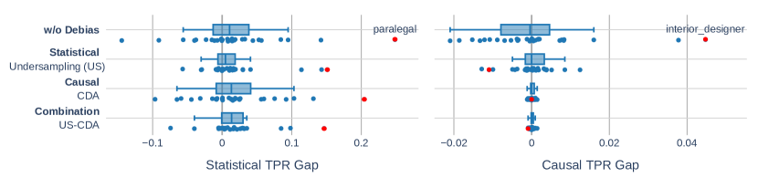
Figure 1: Statistical and causal debiasing methods perform best on the bias metric aligned with their targeted fairness notion. However, CDA is not effective at reducing statistical TPR gap. Our proposed combination approach achieves the best overall results. Results are based on BiasBios dataset with BERT-Base-Uncased model. Section 4 provides details on the experiments.

2 Background

This section provides background on bias metrics based on statistical and causal notions of fairness and overviews bias mitigation techniques.

2.1 Bias Metrics

We consider a model fine-tuned for a classification task where the model $f$ makes predictions $\hat{Y}$ given inputs $X$ and the ground truths are $Y$.

Statistical bias metrics. Statistical bias metrics quantify bias based on statistical fairness (also known as group fairness), which compares prediction outcomes between groups. Common statistical fairness definitions include demographic parity (DP), which requires equal positive prediction rates (PPR) for every group (Barocas et al., 2019). Different from DP, equalized odds consider ground truths and demand equal true positive rates (TPR) and false positive rates (FPR) across groups (Hardt et al., 2016).

Statistical PPR gap ($\mathcal{SG}^{\mathsf{PPR}}$) between binary genders $g$ (female) and $\neg g$ (male) can be defined as (Zayed et al., 2022):

$$\mathbb{E}[\hat{Y}=1\;|\;G=g]-\mathbb{E}[\hat{Y}=1\;|\;G=\neg g]$$

where the model predictions $\hat{Y}$ can be either 0 or 1. If $\mathcal{SG}^{\mathsf{PPR}}>0$, the model produces positive predictions for females more often than for males.

Statistical TPR gap of binary genders for class $y$ can be formulated as (De-Arteaga et al., 2019):

$$\mathcal{SG}^{\mathsf{TPR}}_{y} =\mathsf{TPR}_{s}(g,y)-\mathsf{TPR}_{s}(\neg g,y)$$

$$\mathsf{TPR}_{s}(g,y) =\mathbb{E}[\hat{Y}=y\;|\;G=g,Y=y]$$

A positive $\mathcal{SG}^{\mathsf{TPR}}$ would mean that the model outputs the correct positive prediction for female inputs more often than for male inputs. Statistical FPR gap can be defined analogously as in Equation 1 (Appendix A).

Causal bias metrics. Causality-based bias metrics for NLP models are usually based on counterfactual fairness (Kusner et al., 2017), which requires the model to make the same prediction for the text input even when group identity terms in the input are changed. The evaluation set is usually constructed by perturbing the identity tokens in the inputs from datasets (Prabhakaran et al., 2019; Garg et al., 2019; Qian et al., 2022) or by creating synthetic sentences from templates (Dixon et al., 2018; Lu et al., 2019; Huang et al., 2020).

Following Garg et al. (2019), we can define causal gender gap for an input $x$ as:

$$|f(x\,|\,\mathit{do}(G=g))-f(x\,|\,\mathit{do}(G=\neg g))|$$

where the $\mathit{do}$-operator enforces an intervention on gender. The term $f(x\,|\,\mathit{do}(G=g))$ indicates the model’s prediction for $x$ if the gender of $x$ were set to female. To identify the bias direction, we will consider the causal gap without the absolute value. More information on how we perform gender intervention on texts is given in Appendix B.3.

Causal PPR Gap ($\mathcal{CG}^{\mathsf{PPR}}$) can be estimated by the average causal effect of the protected characteristic on the model’s prediction being positive. (Rubin, 1974; Pearl et al., 2016):

$$\mathbb{E}[\hat{Y}=1\,|\,\mathit{do}(G=g)]-\mathbb{E}[\hat{Y}=1\,|\,\mathit{do}(G=\neg g)]$$

If $\mathcal{CG}^{\mathsf{PPR}}$ is zero, it would mean that gender has no influence on model’s positive prediction outcome. To compare with statistical TPR gap, we formulate causal TPR gap by averaging the TPR difference for each individual:

$$\mathcal{CG}^{\mathsf{TPR}}_{y} =\mathsf{TPR}_{c}(g,y)-\mathsf{TPR}_{c}(\neg g,y)$$

$$\mathsf{TPR}_{c}(g,y) =\mathbb{E}[\hat{Y}=y\,|\,do(G=g),Y=y]$$

Similarly, we can define causal FPR gap as in Equation 2 (Appendix A).

Comparing statistical and causal bias metrics. The key difference between statistical and causal metrics is how the test examples are selected and generated for evaluation. Statistical metrics are based on the original unperturbed examples, while causal metrics consider an additional perturbation process to generate test examples besides the original examples. Proponents of causal metrics argue that statistical metrics are based on observational data, which may contain spurious correlations and therefore cannot determine whether the protected attribute is the reason for the observed statistical differences (Kilbertus et al., 2017; Nabi and Shpitser, 2018). On the other hand, statistical metrics are easy to assess, whereas causal metrics require a counterfactual version of each instance. Due to the discrete nature of texts, we can conveniently generate counterfactuals at the intervention level by perturbing the identity terms in the sentences (Garg et al., 2019). Yet, it is possible to produce ungrammatical or nonsensical sentences using such perturbations (Morris et al., 2020). In addition, changing the identity terms alone may not be enough to hide the identity signals as there could be other terms or linguistic tendencies that are correlated with the target identity. Czarnowska et al. (2021) provides a comprehensive comparison of existing extrinsic bias metrics in NLP.

2.2 Bias Mitigation

Bias mitigation techniques for NLP models can be categorized broadly based on whether the mitigation is done to the training data (pre-processing methods), to the learning process (in-processing), or to the model outputs (post-processing).

Pre-processing methods attempt to mitigate bias by modifying the training data before training. Statistical methods adjust the distribution of the training data through resampling or reweighting. Resampling can be done by either adding examples for underrepresented groups (Dixon et al., 2018; Costa-jussà and de Jorge, 2020) or removing examples for overrepresented groups (Wang et al., 2019; Han et al., 2022). Reweighting assigns a weight to each training example according to the frequency of its class label and protected attribute (Calders et al., 2009; Kamiran and Calders, 2012; Han et al., 2022). Causal methods such as counterfactual data augmentation (CDA) augment the training set with examples substituted with different identity terms (Lu et al., 2019). This is the same as data augmentation based on gender swapping (Zhao et al., 2018; Park et al., 2018). While both statistical and causal methods seek to balance the group distribution, CDA performs interventions on the protected attribute whereas resampling and reweighing do not modify the attribute in the examples. Previous works have also considered removing protected attributes De-Arteaga et al. (2019). However, this “fairness through blindness” approach is ineffective as there may be other proxies correlate with the protected attributes (Chen et al., 2019).

In-processing methods incorporate a fairness constraint in the training process. The constraint can be either based on statistical fairness (Kamishima et al., 2012; Zafar et al., 2017; Donini et al., 2018; Subramanian et al., 2021; Shen et al., 2022b) or causal fairness (Garg et al., 2019). Adversarial debiasing methods train the model jointly with a discriminator network from a typical GAN as an adversary to remove features corresponding to the protected attribute from the intermediate representations (Zhang et al., 2018; Elazar and Goldberg, 2018; Li et al., 2018; Han et al., 2021)

Post-processing methods adjust the outputs of the model at test time to achieve desired outcomes for different groups (Kamiran et al., 2010; Hardt et al., 2016; Woodworth et al., 2017). Zhao et al. (2017) use a corpus-level constraint during inference. Ravfogel et al. (2020) remove protected attribute information from the learned representations.

2.3 Related Work

Garg et al. (2019) is the only work that evaluates NLP models with both statistical and causal bias metrics. They evaluate toxicity classifiers trained with CDA and counterfactual logit pairing and observe a tradeoff between counterfactual token fairness and TPR gaps. Han et al. (2023) is the only work that attempts to achieve both statistical and causal fairness through fair representational learning on tabular data.

Previous work has studied the impossibility theorem of statistical fairness, which states that, for binary classification, equalizing multiple common statistical bias metrics between protected attributes is impossible unless the distribution of outcome is equal for both groups (Kleinberg et al., 2016; Chouldechova, 2017; Bell et al., 2023). While these works focus on tabular data and statistical bias metrics, our work studies statistical and causal bias metrics used for NLP tasks.

Comparison between various bias metrics for NLP models has also been explored. Intrinsic and extrinsic bias metrics have been shown to have no correlation with each other (Delobelle et al., 2022; Cabello et al., 2023). Delobelle et al. (2022) also shows that the measure of intrinsic bias varies depending on the choice of words and templates used for evaluation. Shen et al. (2022a) find no correlation between statistical bias metrics and an adversarial-based bias metric, which measures the leakage of protected attributes from the intermediate representation of a model.

Dwork et al. (2012) proposes individual fairness, which demands similar outcomes to similar individuals. This is similar to counterfactual fairness in the sense that two similar individuals can be considered as counterfactuals of each other (Loftus et al., 2018; Pfohl et al., 2019). The difference is that individual fairness considers similar individuals based on some distance metrics while counterfactual fairness considers a counterfactual example for each individual from a causal perspective. Zemel et al. (2013) proposes learning representations with group information sanitized and individual information preserved to achieve both individual and group (statistical) fairness.

3 Bias Metrics Are Disparate

Disparities between different statistical fairness definitions and group and individual fairness have been studied in the tabular data settings (Section 2.3). We focus on the most common type of bias metrics, statistical and causal, used for evaluating NLP tasks. We first explain why statistical and causal bias metrics may produce inconsistent results. We then report on the experiments to measure disparities between the metrics on evaluating gender bias in an occupation classification task.

3.1 Statistical does not Imply Causal Fairness

While correlation and causation can happen simultaneously, correlation does not imply causation (Fisher, 1958). Correlation refers to the statistical dependence between two variables. Statistical correlation is not causation when there is a confounding variable that influences both variables (Pearl, 2009), leading to spurious correlations (Pearson, 1896).

To equate statistical estimates with causal estimates, the exchangeability assumption must be satisfied (Neal, 2015). This means that the potential outcome of a protected group is independent of the group assignment. The model’s prediction outcome should be the same even when the groups are swapped. One common way to achieve this is through randomized control trials by randomly assigning individuals to different groups (Fisher, 1935), making the groups more comparable. In the case of bias evaluation, it is impossible to assign gender or identity to a person randomly. Furthermore, most data are sampled from the Internet, which does not guarantee diversity and may still encode bias (Bender et al., 2021). Despite the disparities between statistical and causal bias estimation, it does not entail that achieving both statistical and causal fairness is impossible.

3.2 Evaluation

Task. We use the BiasBios dataset (De-Arteaga et al., 2019) comprising nearly 400,000 online biographies of 28 unique occupations scraped from the CommonCrawl. The task is to predict the occupation given in the biography with the occupation title removed. Each biography includes the name and the pronouns of the subject. The gender of the subject is determined by a pre-defined list of explicit gender indicators (Appendix B.3). We use the train-dev-test split of the BiasBios dataset from Ravfogel et al. (2020). We perform a different data pre-processing for the biographies (see Appendix B.2 for details).

Setup. We fine-tune ALBERT-Large (Lan et al., 2020) and BERT-Base-Uncased (Devlin et al., 2019) on the BiasBios dataset with normal training. We then evaluate the models with statistical and causal TPR gap.

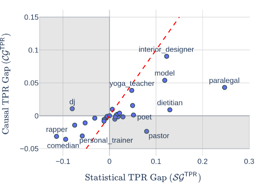
(a) ALBERT-Large

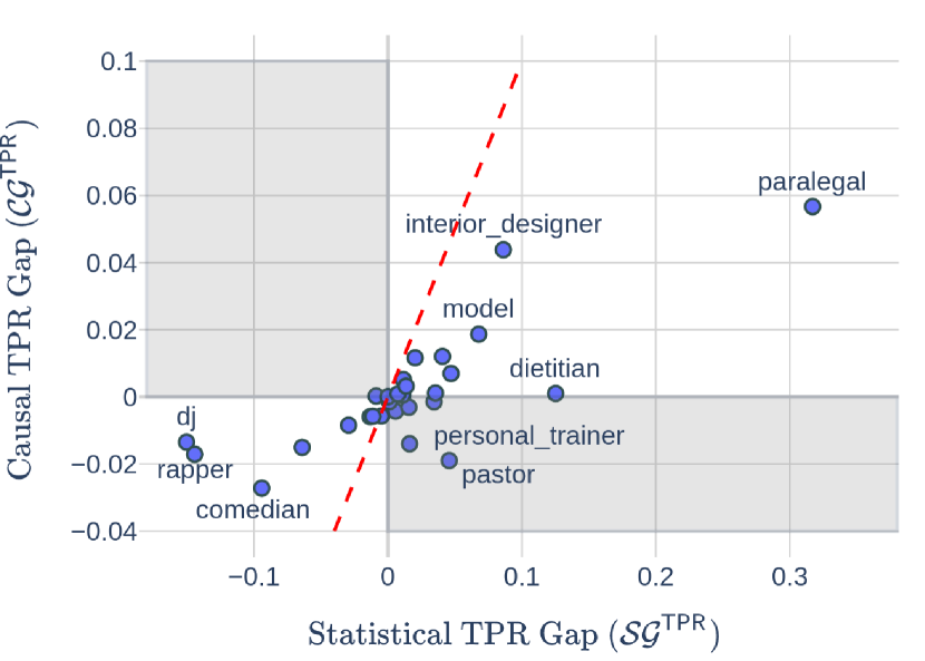
(b) BERT-Base-Uncased

Figure 2: Statistical and causal TPR gaps evaluated on models with normal training. Red dashed line indicates $\mathcal{SG}=\mathcal{CG}$. Shaded areas represent $\mathcal{SG}$ and $\mathcal{CG}$ reporting opposite gender bias direction.

Results. Figure 2 shows the statistical and causal TPR gap for ALBERT and BERT models. Each data point represents the TPR gap of an occupation evaluated over the test examples with the occupation label. The results reveal the disparity between statistical estimation and causal estimation. Most occupations are off the red dashed line where $\mathcal{SG}=\mathcal{CG}$. For nearly all occupations, $\mathcal{CG}$ is closer to zero than $\mathcal{SG}$. In addition, we find a few cases where $\mathcal{SG}$ and $\mathcal{CG}$ show bias in opposite directions such as dj and pastor in 2(a). Similar results are found for statistical and causal FPR gap (see Appendix D).

3.3 Bag-of-Words Analysis

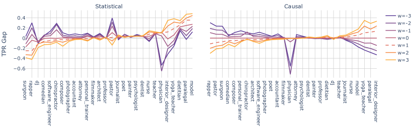
Figure 3: Statistical and causal TPR gap of BoW model per occupation when adjusting both gender token weights. $w=1$ indicates the weight is unchanged. Occupations are sorted by gap with $w=1$. Increasing the magnitude of the gender token weights increases bias on both statistical and causal bias metrics. Yet, $\mathcal{CG}^{\mathsf{TPR}}=0$ when $w=0$.

To test the extent to which statistical and causal bias metrics can capture gender bias we train a Bag-of-Words (BoW) model with logistic regression on the BiasBios dataset where we can intentionally control the model’s bias. We do this by identifying the model weights corresponding to gender signal tokens (Appendix B.3) and multiplying the weights for these tokens by a weight $w$. This allows us to tune the bias of a simple model and see how the different bias metrics measure the resulting bias.

Figure 3 shows $\mathcal{SG}^{\mathsf{TPR}}$ and $\mathcal{CG}^{\mathsf{TPR}}$ of the BoW model when changing the weights for all gender-associated tokens. The magnitude of both bias scores increases as we increase the weighting of the gender tokens. The model is biased in the opposite gender direction when we reverse the weight $w$ by multiplying by a negative value. This demonstrates that both metrics are indeed able to capture bias in the model and, for the most part, reflect the amount of bias in the expected direction. Note that $\mathcal{CG}^{\mathsf{TPR}}=0$ for all occupations when $w=0$. This is because $\mathcal{CG}^{\mathsf{TPR}}$ considers the average difference between pairs of sentences that only differ in tokens representing the gender. When $w=0$, the model would exclude all gender tokens and each sentence pair would render the same to the model. On the other hand, $\mathcal{SG}^{\mathsf{TPR}}$ is nonzero for most occupations when $w=0$, meaning that it captures gender bias beyond explicit gender indicators. This suggests models trained to achieve causal fairness may still be biased toward other implicit gender features not identified in our explicit gender token list.

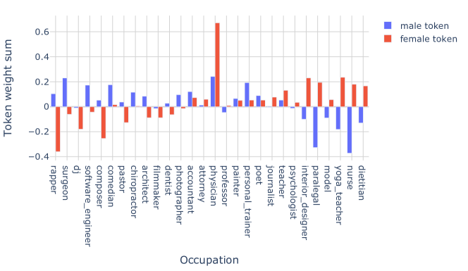
Figure 11: The sum of model weights for male and female gender tokens weighted by the token frequency in test examples of the occupation class.

The spikes in Figure 3 may be attributed to the relatively large gap in token weights between the two genders for predicting the occupation, as shown in Figure 11. The increased TPR gap is particularly significant for occupations with positive token weights for the dominant gender and negative token weights for the other gender, such as rapper and paralegal. In one extreme case, both gender token weights are positive for physician, with female tokens having a lot higher weight value than male tokens. This results in a huge TPR gap increase only in the negative direction when applying a larger negative value of $w$.

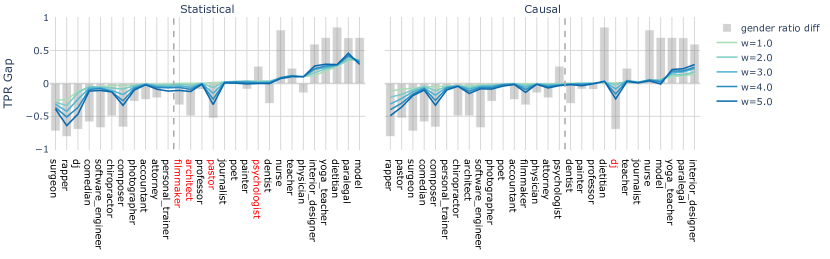
Figure 4: Statistical and causal TPR gap of BoW model per occupation when increasing female token weights in the model. The occupations highlighted in red demonstrate an increased TPR gap toward the opposite bias direction. The grey dashed line shows where the gap is zero when $w=1$. The grey bars are the gender ratio difference of the occupation in the training set.

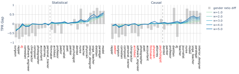
Figure 10: Statistical and causal TPR gaps of BoW model for each occupation when increasing the male token weights. Occupations are sorted by gap with $w=1$.

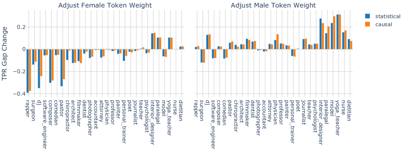
Figure 12: The TPR gap difference when increasing either female or male token weights from $w=1$ to $w=5$. Both metrics show similar patterns of TPR gap change for all occupations.

We further analyze how model weights of individual gender affect bias scores. Figure 4 shows the statistical and causal TPR gap of each occupation when increasing female token weights, and Figure 10 (in Appendix D.2) shows the results of increasing male token weights. We observed that increasing female token weights has a greater effect on increasing the TPR gap of male-biased occupations (on the left side of the grey dashed line in Figure 4), and vice versa. In addition, some occupations (as highlighted in red) show an increased TPR gap to the opposite gender bias direction of their bias scores indicated by the metric when $w=1$. For instance, filmmaker, architect, and pastor are female-biased based on the statistical metric but become male-biased when increasing the female token weights due to their negative weight values (Figure 11). We find that these occupations are the ones that the two metrics contradict in the bias direction (Table 3). However, both metrics show similar patterns and directions of TPR gap increase across occupations (Figure 12). The only difference is the starting point of TPR gap score when $w=1$.

4 Cross-Evaluation

This section cross-evaluates the effectiveness of existing debiasing methods on gender bias in an occupation classification and toxicity detection task. We show using statistical and causal debiasing methods alone may not achieve both types of fairness.

4.1 Setup

We focus on pre-processing methods since Shen et al. (2022b) found that resampling and reweighting achieve better statistical fairness than the in-processing and post-processing methods. For the statistical methods, we apply both resampling using oversampling (OS) and undersampling (US) and reweighting (RW) using the weight calculation from Kamiran and Calders (2012). For the causal methods, we fine-tune the model with CDA.

We apply each debiasing method to the ALBERT-Large (Lan et al., 2020) and BERT-Base-Uncased (Devlin et al., 2019) models. We also include experiments with Zari (Webster et al., 2020), which is an ALBERT-Large model pre-trained with CDA. To consider the effect of CDA during pre-training alone and during both pre-training and fine-tuning, we fine-tune Zari with normal training and CDA. Training details are provided in Appendix E.

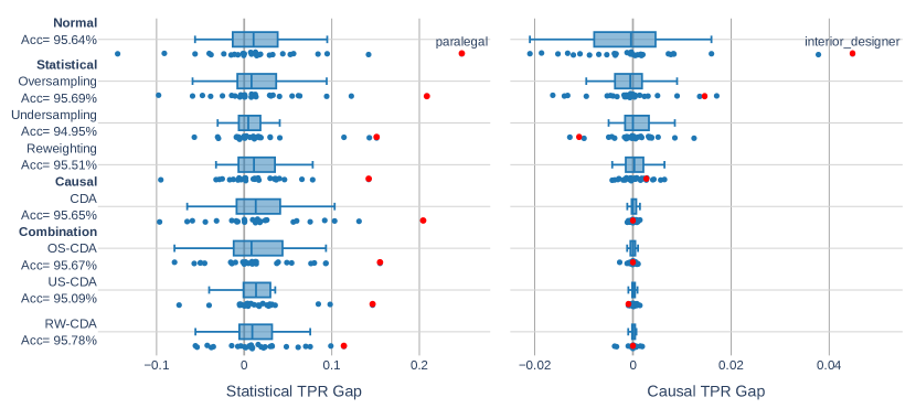
Figure 5: Statistical and causal TPR gap per occupation evaluated on BERT-Base-Uncased model, averaged over 3 different runs. Each data point is computed over test examples labeled with the same occupation. We show outliers for normal training in red dots and how their values change with different debiasing methods. Statistical and causal debiasing methods perform better on the metric they are targeting, but may not reduce bias on the other metric. Our proposed methods, US-CDA and RW-CDA, achieve the best overall performance.

4.2 Tasks

We test all the models on two benchmark tasks for bias detection: occupation classification and toxicity detection.

Occupation Classification. We use the BiasBios dataset introduced in Section 3.2. We evaluate gender bias with TPR and FPR gap based on both statistical and causal notions of fairness as defined in Section 2.1. Since the BiasBios dataset contains multiple classes, we follow Romanov et al. (2019) and compute a single score that quantifies overall gender bias. For each bias metric $\mathit{M}$ (e.g., $\mathcal{SG}^{\mathsf{TPR}}_{g,y}$), we compute the root mean square of the bias score across all occupation classes $Y$:

$$\mathit{RMS}_{\mathit{M}}=\sqrt{\frac{1}{|Y|}\sum_{y\in Y}(\mathit{M}_{y})}$$

where $\mathit{M}_{y}$ is the bias score for occupation $y$ computed with $\mathit{M}$.

Toxicity Detection. We use the Jigsaw dataset consisting of approximately 1.8M comments taken from the Civil Comments platform. The task is to predict the toxicity score of each comment. For our experiments, we use binary toxicity labels, toxic and non-toxic. In addition to the toxicity score, a subset of examples are labeled with the identities mentioned in the comment. We only select the examples labeled with female and male identities and with high annotator agreement on the gender identity labels. Since some examples contain a mix of genders, we assign the gender to each example based on the gender labeled with the highest agreement. To perform gender intervention with CDA, we use the gender-bender Python package to generate counterfactual examples . Appendix C.1 provides details on how we preprocess the data. Following Zayed et al. (2022), we compute statistical and causal PPR gap. As female and male groups do not have the same label distribution, the PPR gap of a perfect predictor will be non-zero. Therefore, we also compute statistical and causal TPR gap for toxic and non-toxic classes.

4.3 Results

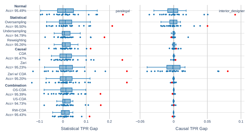
Figure 6: Statistical and causal TPR gap per occupation results for ALBERT-Large, averaged over 3 different runs.

Occupation classification. Figure 5 and Figure 6 show statistical and causal TPR gap per occupation evaluated on BERT and ALBERT models with each debiasing method. Causal debiasing methods show greater effectiveness when evaluated with the causal metric (we discuss the combination methods included in these figures in Section 5). Fine-tuning with CDA reduces $\mathcal{CG}^{\mathsf{TPR}}$ to nearly zero for all occupations, but does not produce any significant reduction for $\mathcal{SG}^{\mathsf{TPR}}$. On the other hand, Zari exhibits higher statistical and causal gap than performing CDA during fine-tuning (Figure 6). Thus, using CDA during pre-training alone is insufficient to reduce bias. Statistical debiasing methods such as undersampling and reweighting reduce bias on both statistical and causal metrics, though the bias reduction on the causal metric is not as significant as CDA. We find that oversampling is less effective than other statistical debiasing methods on both metrics. We found similar results with statistical and causal FPR gaps (Appendix F.2).

Toxicity detection. Table 1 shows the bias evaluation results for the BERT model trained with different debiasing methods on the Jigsaw dataset. We find that statistical and causal bias metrics sometimes disagree on which gender the model is biased toward. Similar to the results for the BiasBios task, statistical and causal debiasing methods do particularly well on the bias metrics based on their targeted fairness definition. However, they increase bias on metrics that use the other type of fairness notion. Similar results are found for ALBERT model (Appendix G.1).

Method	$\mathcal{SG}^{\mathsf{PPR}}$	$\mathcal{CG}^{\mathsf{PPR}}$	$\mathcal{SG}^{\mathsf{TPR}}_{y=1}$	$\mathcal{CG}^{\mathsf{TPR}}_{y=1}$	$\mathcal{SG}^{\mathsf{TPR}}_{y=0}$	$\mathcal{CG}^{\mathsf{TPR}}_{y=0}$
Normal	$-2.79$$\pm$$0.28$	$0.89$$\pm$$0.10$	$-2.77$$\pm$$0.67$	$2.33$$\pm$$1.06$	$1.28$$\pm$$0.30$	$-0.73$$\pm$$0.11$
CDA	$-3.02$$\pm$$0.23$	$0.25$$\pm$$0.08$	$-2.62$$\pm$$2.07$	$0.36$$\pm$$0.57$	$1.52$$\pm$$0.29$	$-0.24$$\pm$$0.06$
OS	$-1.21$$\pm$$0.22$	$1.33$$\pm$$0.31$	$2.21$$\pm$$0.35$	$5.24$$\pm$$0.42$	$0.20$$\pm$$0.17$	$-0.88$$\pm$$0.30$
US	$-1.54$$\pm$$0.26$	$1.67$$\pm$$0.29$	$1.61$$\pm$$1.11$	$4.56$$\pm$$0.63$	$0.37$$\pm$$0.24$	$-1.34$$\pm$$0.26$
RW	$-1.44$$\pm$$0.31$	$1.44$$\pm$$0.24$	$2.09$$\pm$$0.85$	$4.92$$\pm$$0.53$	$0.39$$\pm$$0.26$	$-1.05$$\pm$$0.25$
OS-CDA	$-2.09$$\pm$$0.30$	$0.18$$\pm$$0.16$	$-1.11$$\pm$$0.99$	$0.39$$\pm$$0.46$	$0.79$$\pm$$0.28$	$-0.15$$\pm$$0.15$
US-CDA	$-1.90$$\pm$$0.19$	$0.11$$\pm$$0.11$	$-1.66$$\pm$$1.88$	$0.14$$\pm$$0.70$	$0.57$$\pm$$0.26$	$-0.11$$\pm$$0.06$
RW-CDA	$-1.76$$\pm$$0.36$	$0.33$$\pm$$0.11$	$0.56$$\pm$$1.27$	$1.08$$\pm$$0.74$	$0.62$$\pm$$0.40$	$-0.24$$\pm$$0.10$

Table 1: Bias evaluation results evaluated on the Jigsaw dataset with BERT-Base-Uncased model. The results shown are averaged over 5 different runs. All values are on a log scale with base $10^{-2}$.

5 Achieving Both Statistical and Causal Fairness

In the previous section, we saw that using either statistical or causal debiasing method alone may not achieve both statistical and causal fairness. To counter this problem, this section considers simple methods that combine both statistical and causal debiasing techniques.

5.1 Composed Debiasing Methods

We introduce three approaches that combine techniques from both statistical and causal debiasing:

Resampling with CDA. OS-CDA and US-CDA combines resampling methods (oversampling and undersampling) with CDA. For Biasbios, we first perform resampling on the training set, then augment the resampled set with CDA. For Jigsaw, we balance the original examples based on the original gender and the counterfactual examples based on the counterfactual gender.

Reweighting with CDA. RW-CDA applies CDA on the training set and fine-tunes the model with reweighting. For BiasBios, we use the same weight computed on the original training set for both the original and its counterfactual pair. For Jigsaw, we use weight of 1 for all counterfactual examples.

We use different combination strategies for the two datasets as we noticed the methods used for BiasBios do not work well on the Jigsaw dataset. This may be due to the mix of genders in a subset of examples in the Jigsaw dataset. The gender signals in the examples may be flipped after performing CDA. We provide performance comparisons between the different combination strategies we have tried on the Jigsaw task in Appendix G.2.

5.2 Results

Figure 5 and Figure 6 show statistical and causal TPR gap per occupation evaluated on the BiasBios dataset for BERT and ALBERT models. The combined methods US-CDA and RW-CDA are more effective at reducing bias on both metrics compared to other methods. To compare overall performance, we show the root mean square of each bias metric in Table 4 and Table 5 (both in Appendix F.1). All three combination approaches perform better on $\mathcal{CG}^{\mathsf{TPR}}$ compared to using a statistical or causal debiasing method alone. OS-CDA and US-CDA also reduce bias on $\mathcal{SG}^{\mathsf{TPR}}$ (11–16% decrease) and $\mathcal{SG}^{\mathsf{FPR}}$ (1–8% decrease), comparing to their statistical debiasing counterparts. RW-CDA achieves comparable performance on $\mathcal{SG}$ to reweighting. Undersampling and US-CDA sacrifice the general performance with a decrease of around 0.7% in accuracy compared to other methods, which preserve the baseline accuracy within 0.3%.

Table 1 and Table 6 (Appendix G.1) report the results of BERT and ALBERT models for the Jigsaw dataset. While statistical and causal debiasing methods only improve one type of bias metric and worsen the other, our proposed combination approaches are able to reduce bias on both types of bias metrics. The combined methods OS-CDA and US-CDA perform better than CDA on all causal bias metrics. RW-CDA performs better on $\mathcal{SG}$ but is less effective at reducing bias on $\mathcal{CG}$ compared to the other combination approaches.

6 Summary

We demonstrate the disparities between statistical and causal bias metrics and provide insight into how and why optimizing based on one type of metric does not necessarily improve the other. We show this by cross-evaluating existing statistical and causal debiasing methods on both metrics and find that they sometimes may even worsen the other type of bias metrics. To obtain models that perform well on both types of bias metrics, we introduce simple debiasing strategies that combine both statistical and causal debiasing techniques.

Limitations

Due to the limited benchmark datasets compatible with extrinsic metrics (Orgad and Belinkov, 2022), we only conduct experiments on two gender bias tasks. Further testing is needed to determine if the bias metric disparities are present in other tasks and whether our proposed debiasing methods can still be effective. The gender intervention method used for counterfactual data augmentation is based on a predefined list of gender tokens, which may not cover all possible tokens representing gender. In addition, our experiments exclusively focus on binary-protected attributes. Future work should explore how to generalize our results to tasks with non-binary protected attributes. While our proposed debiasing methods are able to reduce bias on both statistical and causal bias metrics, there is room for improvements in the statistical bias metrics when compared to statistical debiasing methods. Future work could consider other types of debiasing techniques beyond pre-processing-based methods. For instance, in-processing methods can be adapted by enforcing both statistical and causal fairness constraints during training.

Appendix A False Positive Rate Gap

Statistical FPR gap between binary gender $g$ (female) and $\neg g$ (male) for class $y$ is defined as:

$$\mathcal{SG}^{\mathsf{FPR}}_{y} =\mathsf{FPR}_{s}(g,y)-\mathsf{FPR}_{s}(\neg g,y)$$ (1)

$$\mathsf{FPR}_{s}(g,y) =\mathbb{E}[\hat{Y}=y\;|\;G=g,Y\not=y]$$

Causal FPR gap is computed by averaging the FPR difference for each individual:

$$\mathcal{CG}^{\mathsf{FPR}}_{y} =\mathsf{FPR}_{c}(g,y)-\mathsf{FPR}_{c}(\neg g,y)$$ (2)

$$\mathsf{TPR}_{c}(g,y) =\mathbb{E}[\hat{Y}=y\,|\,do(G=g),Y\not=y]$$

Appendix B BiasBios Dataset Details

B.1 Dataset Statistics

The dataset contains 255,707 training examples, 39,369 validation examples, and 98,339 testing examples. Figure 7 shows the full list of occupations and their gender frequency in the BiasBios training set. The gender and occupation distribution for validation and testing sets are similar to the training set.

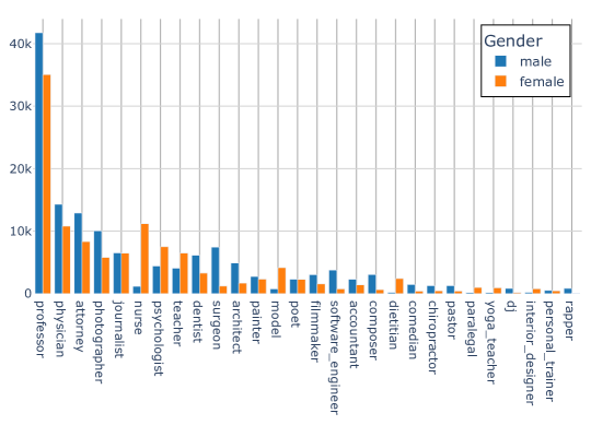
Figure 7: Gender frequency for each occupation in the training set.

B.2 Dataset Construction

The original BiasBios dataset consists of extracted biographies with the first sentences removed from each biography as they include the occupation titles corresponding to the ground truth labels. We notice a lot of the important information is in the first sentences and it is hard to correctly identify the occupation of some examples without the first sentences even for humans. Thus, we keep the first sentence but replace any occupation tokens that appear in the biography with an underscore (e.g., "Alice is a nurse working at a hospital" to "Alice is a _ working at a hospital"). We notice that our model performance is higher than the same model trained on the original dataset (Webster et al., 2020). This can be attributed to having longer sequences and more context information in the inputs.

B.3 Gender Intervention

To perform gender intervention, we first identify words with explicit gender indicators in the input. If the assigned gender value is different from the original input, we swap the identified words with the corresponding words in the mapping with an opposite gender. We use the same list of explicit gender indicators used in BiasBios dataset and perform gender mapping as follows:

• Bidirectional: he $\leftrightarrow$ she, himself $\leftrightarrow$ herself, mr $\leftrightarrow$ ms

• Unidirectional: hers $\rightarrow$ his, his $\rightarrow$ her, him $\rightarrow$ her, her $\rightarrow$ his or him, mrs $\rightarrow$ mr

Words in blue are associated with male gender and words in red are associated with female gender. Since "her" can be mapped to either "his" or "him" depending on the context, we use Part-of-Speech tagging to determine which one to map to.

Appendix C Jigsaw Dataset Details

C.1 Dataset Construction

Each comment is associated with a toxicity label and several identity labels. The label values range from 0.0 to 1.0 representing the percentage of annotators who agreed that the label fit the comment. We binarized the toxicity values and considered comments as toxic if their toxicity values exceeded 0.5. We assigned female gender to an example if its female identity label value is higher than the male one and assigned male gender vice versa. To make better differentiation between the two genders, we filtered out examples if the difference between male and female label values is smaller or equal to 0.5. We use train.csv from the Kaggle competition for training and validation with an 80/20 split. We use test_public_expanded.csv and test_private_expanded.csv for testing.

Label	Gender	Count	Percentage (%)
Toxic	F	2504	5.89
Toxic	M	2123	4.99
Non-Toxic	F	22,465	52.83
Non-Toxic	M	15,431	26.29

Table 2: Gender and label distribution of Jigsaw training set.

C.2 Dataset Statistics

The final dataset after pre-processing contains 42,523 training examples, 10,631 validation examples, and 5,448 testing examples. Table 2 shows the gender and label distribution on the training set. All three data splits have similar distributions. We also show the distribution of the gender label values in Figure 8. For examples that contain a mix of both female and male genders, we show the gender label value of the final gender we assigned (the gender with a higher label value).

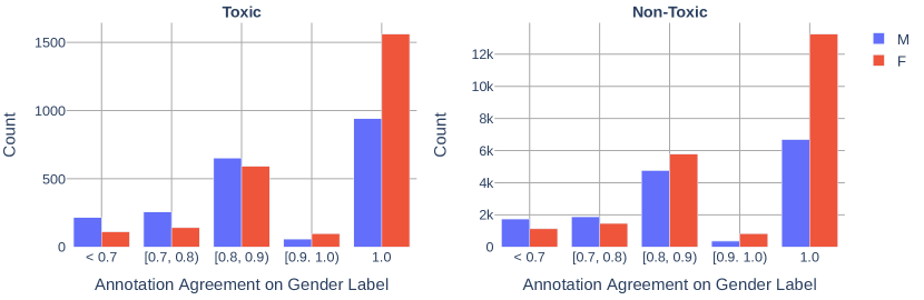
Figure 8: Distribution of annotation agreement on the gender labels. 1.0 indicates all annotators agree that the gender is mentioned in the comment.

Appendix D Disparities between Statistical and Causal Bias Metrics

D.1 Statistical vs Causal FPR Gap

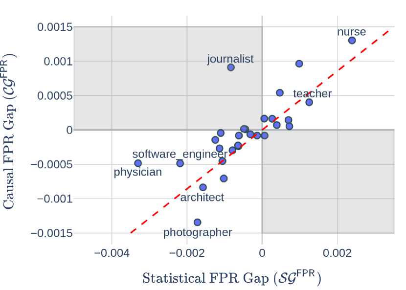
(a) ALBERT-Large

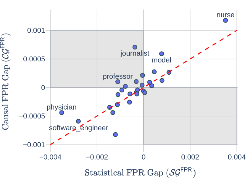
(b) BERT-Base-Uncased

Figure 9: Statistical and causal FPR gap on ALBERT-Large and BERT-Base-Uncased models with normal training. Red dashed line indicates $\mathcal{SP}=\mathcal{CP}$. Shaded areas represent $\mathcal{SP}$ and $\mathcal{CP}$ reporting opposite gender bias direction.

D.2 BoW Analysis

Occupation	$\mathcal{SG}^{\mathsf{TPR}}$	$\mathcal{CG}^{\mathsf{TPR}}$	Diff	Gender ratio diff in train set
dj	-0.115	0.008	0.123	-0.695
physician	0.105	-0.005	0.110	-0.140
pastor	0.013	-0.088	0.101	-0.523
psychologist	0.036	-0.003	0.039	0.260
poet	0.028	-0.010	0.038	-0.008
architect	0.002	-0.030	0.033	-0.490
filmmaker	0.02	-0.009	0.011	-0.325

Table 3: Occupations where statistical and causal TPR gap shows contradictory bias direction.

Appendix E Training Details

Computing Infrastructure. All the models were trained on 4 Nvidia RTX 2080Ti GPUs.

BiasBios Dataset. We trained all the models with a learning rate of 2e-5 and batch size of 64. We fine-tuned the models for 5-8 epochs with early stopping and choose the model checkpoints with the best validation accuracy. Most models reach the best validation accuracy before epoch 5. We notice that ALBERT with subsampling requires training a few epochs longer than other models to reach comparable performance due to the downsized training data.

Jigsaw Dataset. We trained all the models with a learning rate of 1e-5 and batch size of 128 for 4 epochs with early stopping. Most models converge after 2-3 epochs.

Appendix F BiasBios Results

F.1 Overall Bias Scores

		$\mathcal{SG}$		$\mathcal{CG}$
Method	Acc (%)	$\mathsf{TPR}$	$\mathsf{FPR}$	$\mathsf{TPR}$	$\mathsf{FPR}$
Normal	$95.49$$\pm$$0.13$	$7.853$$\pm$$0.761$	$0.127$$\pm$$0.009$	$2.569$$\pm$$0.509$	$0.051$$\pm$$0.005$
OS	$95.50$$\pm$$0.04$	$6.430$$\pm$$0.172$	$0.115$$\pm$$0.004$	$1.590$$\pm$$0.035$	$0.041$$\pm$$0.003$
US	$94.79$$\pm$$0.08$	$5.600$$\pm$$0.422$	$0.097$$\pm$$0.005$	$0.529$$\pm$$0.402$	$0.011$$\pm$$0.005$
RW	$95.26$$\pm$$0.06$	$4.269$$\pm$$0.427$	$0.085$$\pm$$0.011$	$0.391$$\pm$$0.094$	$0.010$$\pm$$0.001$
CDA	$95.47$$\pm$$0.09$	$7.266$$\pm$$0.870$	$0.113$$\pm$$0.007$	$0.207$$\pm$$0.043$	$0.003$$\pm$$0.000$
Zari	$95.23$$\pm$$0.09$	$8.353$$\pm$$0.550$	$0.132$$\pm$$0.006$	$2.849$$\pm$$0.341$	$0.067$$\pm$$0.005$
Zari w/ CDA	$95.20$$\pm$$0.01$	$7.559$$\pm$$0.787$	$0.119$$\pm$$0.008$	$0.216$$\pm$$0.048$	$0.004$$\pm$$0.001$
OS-CDA	$95.39$$\pm$$0.13$	$5.403$$\pm$$0.176$	$0.109$$\pm$$0.006$	$0.130$$\pm$$0.020$	$0.013$$\pm$$0.011$
US-CDA	$94.73$$\pm$$0.09$	$4.969$$\pm$$0.230$	$0.096$$\pm$$0.015$	$0.174$$\pm$$0.051$	$0.007$$\pm$$0.009$
RW-CDA	$95.43$$\pm$$0.11$	$4.300$$\pm$$0.424$	$0.095$$\pm$$0.011$	$0.137$$\pm$$0.020$	$0.008$$\pm$$0.004$

Table 4: Root mean square of bias metrics for ALBERT-Large model fine-tuned with different debiasing methods. The results shown are averaged over 3 different runs. $\mathcal{SG}$ and $\mathcal{CG}$ are on a log scale with base $10^{-2}$.

		$\mathcal{SG}$		$\mathcal{CG}$
Method	Acc (%)	$\mathsf{TPR}$	$\mathsf{FPR}$	$\mathsf{TPR}$	$\mathsf{FPR}$
Baseline	$95.64$$\pm$$0.02$	$7.472$$\pm$$0.898$	$0.129$$\pm$$0.004$	$1.456$$\pm$$0.271$	$0.033$$\pm$$0.005$
OS	$95.69$$\pm$$0.17$	$6.161$$\pm$$0.282$	$0.116$$\pm$$0.018$	$0.805$$\pm$$0.134$	$0.029$$\pm$$0.008$
US	$94.95$$\pm$$0.19$	$5.257$$\pm$$0.865$	$0.108$$\pm$$0.017$	$0.595$$\pm$$0.083$	$0.023$$\pm$$0.000$
RW	$95.51$$\pm$$0.06$	$4.630$$\pm$$0.288$	$0.096$$\pm$$0.008$	$0.377$$\pm$$0.074$	$0.014$$\pm$$0.004$
CDA	$95.65$$\pm$$0.08$	$6.490$$\pm$$1.159$	$0.109$$\pm$$0.011$	$0.138$$\pm$$0.046$	$0.002$$\pm$$0.001$
OS-CDA	$95.67$$\pm$$0.09$	$5.485$$\pm$$0.327$	$0.106$$\pm$$0.022$	$0.121$$\pm$$0.033$	$0.005$$\pm$$0.003$
US-CDA	$95.09$$\pm$$0.12$	$4.673$$\pm$$0.270$	$0.104$$\pm$$0.007$	$0.131$$\pm$$0.012$	$0.009$$\pm$$0.002$
RW-CDA	$95.78$$\pm$$0.07$	$4.601$$\pm$$0.190$	$0.102$$\pm$$0.002$	$0.148$$\pm$$0.021$	$0.004$$\pm$$0.003$

Table 5: Root mean square of bias metrics for BERT-Base-Uncased model fine-tuned with different debiasing methods. The values shown are averaged over 3 different runs on a log scale with base $10^{-2}$.

F.2 Statistical vs Causal FPR Gap

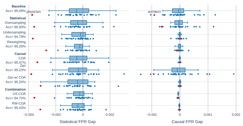
(a) ALBERT-Large

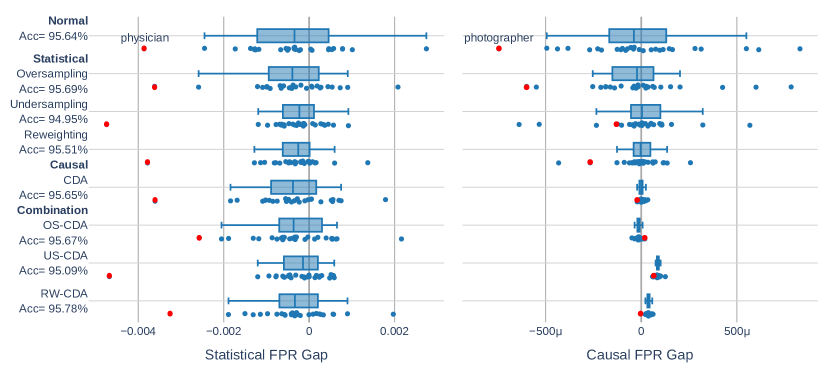
(b) BERT-Base-Uncased

Figure 13: Statistical and Causal FPR gap per occupation, averaged over 3 different runs. Each data point is computed over test examples labeled with the same occupation. We show the outliers for normal training in red dots and how their values change with different debiasing methods. Causal-based debiasing methods perform particularly better on the causal FPR gap while statistical-based debiasing methods are able to reduce bias based on both metrics.

F.3 Correlation to Gender Imbalances in Training Data

In Figure 14, we compare the statistical and causal TPR gap to the female ratio in the training data for each occupation. Both bias metrics show a positive correlation with the gender distribution in the training data. This observation is consistent with the results found in De-Arteaga et al. (2019), where they measure the statistical TPR gap on non-transformer-based models such as BoW.

(a) ALBERT Large

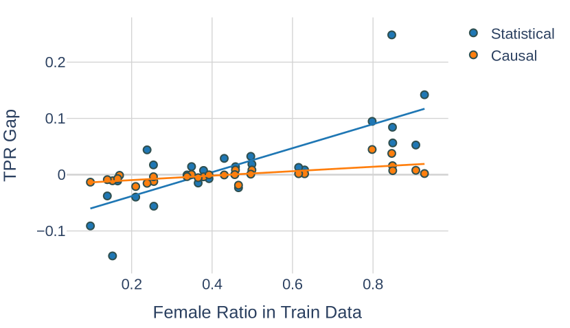
(b) BERT Base Uncased

Figure 14: Statistical and causal TPR gap versus the female ratio of each occupation in the training data.

Appendix G Jigsaw Results

G.1 Overall Bias Scores for ALBERT Model

Method	$\mathcal{SG}^{\mathsf{PPR}}$	$\mathcal{CG}^{\mathsf{PPR}}$	$\mathcal{SG}^{\mathsf{TPR}}_{y=1}$	$\mathcal{CG}^{\mathsf{TPR}}_{y=1}$	$\mathcal{SG}^{\mathsf{TPR}}_{y=0}$	$\mathcal{CG}^{\mathsf{TPR}}_{y=0}$
Normal	$-2.73$$\pm$$0.42$	$0.42$$\pm$$0.21$	$-4.60$$\pm$$3.65$	$1.90$$\pm$$1.37$	$1.21$$\pm$$0.45$	$-0.25$$\pm$$0.08$
CDA	$-3.14$$\pm$$0.59$	$0.20$$\pm$$0.08$	$-3.56$$\pm$$3.08$	$0.86$$\pm$$0.67$	$1.66$$\pm$$0.36$	$-0.13$$\pm$$0.07$
Zari w/ CDA	$-2.89$$\pm$$0.98$	$-0.05$$\pm$$0.12$	$-5.68$$\pm$$2.10$	$-0.32$$\pm$$0.57$	$1.31$$\pm$$0.92$	$0.02$$\pm$$0.07$
US	$-2.37$$\pm$$0.58$	$1.00$$\pm$$0.10$	$-2.57$$\pm$$2.75$	$4.20$$\pm$$0.82$	$1.03$$\pm$$0.45$	$-0.63$$\pm$$0.08$
RW	$-1.70$$\pm$$0.21$	$0.95$$\pm$$0.25$	$-2.07$$\pm$$2.15$	$4.13$$\pm$$0.30$	$0.39$$\pm$$0.29$	$-0.58$$\pm$$0.28$
OS	$-1.79$$\pm$$0.24$	$0.81$$\pm$$0.22$	$-3.18$$\pm$$2.75$	$3.99$$\pm$$0.80$	$0.48$$\pm$$0.22$	$-0.45$$\pm$$0.21$
OS-CDA	$-2.29$$\pm$$0.42$	$0.01$$\pm$$0.11$	$-3.40$$\pm$$2.74$	$0.29$$\pm$$0.69$	$0.83$$\pm$$0.30$	$0.02$$\pm$$0.06$
US-CDA	$-2.22$$\pm$$0.23$	$0.08$$\pm$$0.10$	$-2.57$$\pm$$2.60$	$0.36$$\pm$$0.25$	$0.88$$\pm$$0.30$	$-0.05$$\pm$$0.11$
RW-CDA	$-1.96$$\pm$$0.25$	$0.24$$\pm$$0.09$	$-1.98$$\pm$$1.36$	$0.97$$\pm$$0.73$	$0.76$$\pm$$0.25$	$-0.16$$\pm$$0.07$

Table 6: Bias evaluation results evaluated on the Jigsaw dataset with ALBERT-Large model. The results shown are averaged over 5 different runs. All values are on a log scale with base $10^{-2}$.

G.2 Combination Strategies Comparison

Table 7 shows the performance of two different strategies of combining resampling and CDA. Resample $\rightarrow$ CDA performs resampling first, then applies CDA on the resampled set. CDA $\rightarrow$ Resample performs CDA first, then resamples the original and the counterfactual sets separately. The original examples are resampled based on the original gender distribution. The counterfactual examples are resampled based on their counterfactual genders (not the gender of the original example they originated from). The difference between the two methods is that Resample $\rightarrow$ CDA uses the original gender label for both original and counterfactual examples while CDA $\rightarrow$ Resample considers the counterfactual gender for the counterfactual examples during resampling. We find that the second method performs better on $\mathcal{SG}^{\mathsf{PPR}}$ but increases $\mathcal{CG}^{\mathsf{PPR}}$ compared to the first method. The increase in the causal bias metric may be due to separate resampling on original and counterfactual sets, meaning that some of them may not come in pairs. Nonetheless, the performance still exceeds CDA.

		BERT-Base-Uncased		ALBERT-Large
Strategy	Method	$\mathcal{SG}^{\mathsf{PPR}}$	$\mathcal{CG}^{\mathsf{PPR}}$	$\mathcal{SG}^{\mathsf{PPR}}$	$\mathcal{CG}^{\mathsf{PPR}}$
Resample $\rightarrow$ CDA	OS-CDA	$-2.73$$\pm$$0.72$	$0.011$$\pm$$0.086$	$-2.51$$\pm$$0.49$	$0.004$$\pm$$0.082$
	US-CDA	$-2.12$$\pm$$0.51$	$0.117$$\pm$$0.114$	$-2.88$$\pm$$0.78$	$0.022$$\pm$$0.134$
CDA $\rightarrow$ Resample	OS-CDA	$-2.09$$\pm$$0.30$	$0.176$$\pm$$0.160$	$-2.29$$\pm$$0.42$	$0.015$$\pm$$0.107$
	US-CDA	$-1.90$$\pm$$0.19$	$0.114$$\pm$$0.113$	$-2.22$$\pm$$0.23$	$0.084$$\pm$$0.096$

Table 7: Debiasing performance between two different strategies of combining resampling and CDA. The results shown are evaluated on the BERT model, averaged over 5 different runs. $\mathcal{SG}^{\mathsf{PPR}}$ and $\mathcal{CG}^{\mathsf{PPR}}$ are on a log scale with base $10^{-2}$.

Table 8 shows the performance of using different reweighting strategies on counterfactual examples for RW-CDA. We tried RW-CDA method for training on BiasBios dataset, which uses the same weight for both the original and counterfactual examples (first row in Table 8). It is not effective at reducing $\mathcal{SG}^{\mathsf{PPR}}$, but very effective on $\mathcal{CG}^{\mathsf{PPR}}$. We think it may be due to the gender signals of some examples being flipped by CDA. We then tried using weights that correspond to the counterfactual gender for the counterfactual examples. This decreases bias on $\mathcal{SG}^{\mathsf{PPR}}$, but increases bias on $\mathcal{CG}^{\mathsf{PPR}}$. We found that setting the weight to 1 for all counterfactual examples gives the best overall balance between $\mathcal{SG}^{\mathsf{PPR}}$ and $\mathcal{CG}^{\mathsf{PPR}}$. It also outperforms other strategies on $\mathcal{SG}^{\mathsf{PPR}}$.

	BERT-Base-Uncased		ALBERT-Large
Strategy	$\mathcal{SG}^{\mathsf{PPR}}$	$\mathcal{CG}^{\mathsf{PPR}}$	$\mathcal{SG}^{\mathsf{PPR}}$	$\mathcal{CG}^{\mathsf{PPR}}$
Same weight	$-2.30$$\pm$$0.35$	$0.162$$\pm$$0.109$	$-2.41$$\pm$$0.30$	$0.070$$\pm$$0.059$
Counterfactual gender weight	$-1.82$$\pm$$0.36$	$0.653$$\pm$$0.242$	$-2.19$$\pm$$0.31$	$0.371$$\pm$$0.063$
Weight=1	$-1.76$$\pm$$0.36$	$0.327$$\pm$$0.110$	$-1.96$$\pm$$0.25$	$0.239$$\pm$$0.091$

Table 8: Debiasing performance of different reweighting strategies on counterfactual examples for RW-CDA. The results shown are evaluated on the BERT model, averaged over 5 different runs. $\mathcal{SG}^{\mathsf{PPR}}$ and $\mathcal{CG}^{\mathsf{PPR}}$ are on a log scale with base $10^{-2}$.

G.3 General Performance

Method	AUC (ALBERT)	AUC (BERT)
Normal	$0.930$$\pm$$0.002$	$0.925$$\pm$$0.003$
CDA	$0.930$$\pm$$0.002$	$0.928$$\pm$$0.002$
Zari w/ CDA	$0.928$$\pm$$0.005$	—
OS	$0.931$$\pm$$0.001$	$0.932$$\pm$$0.002$
US	$0.929$$\pm$$0.003$	$0.924$$\pm$$0.004$
RW	$0.930$$\pm$$0.005$	$0.929$$\pm$$0.003$
OS-CDA	$0.930$$\pm$$0.003$	$0.931$$\pm$$0.002$
US-CDA	$0.929$$\pm$$0.003$	$0.931$$\pm$$0.002$
RW-CDA	$0.929$$\pm$$0.002$	$0.930$$\pm$$0.003$

Table 9: AUC scores of different debiasing methods. The results shown are averaged over 5 different runs.

G.4 Gender Label Annotation Agreement

We test if gender label annotation agreement in the Jigsaw dataset has an effect on the bias scores. In Figure 15, we show statistical and causal PPR gap of examples with different range of annotation agreement for each debiasing methods. All methods have the highest score of statistical PPR gap at [0.85, 0.96) including the normal training method and have the lowest score when annotation agreement >=0.95. On the other hand, causal PPR gap of each debiasing method remain similar at different range of gender annotation agreement.

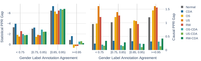
(a) BERT-Base-Uncased

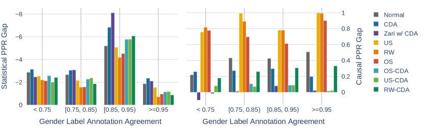
(b) ALBERT-Large

Figure 15: Statistical and Causal PPR Gap of examples with different range of gender label annotation agreement.

References

- Barocas et al. (2019) Solon Barocas, Moritz Hardt, and Arvind Narayanan. 2019. Fairness and Machine Learning: Limitations and Opportunities. fairmlbook.org. http://www.fairmlbook.org.
- Bell et al. (2023) Andrew Bell, Lucius Bynum, Nazarii Drushchak, Tetiana Zakharchenko, Lucas Rosenblatt, and Julia Stoyanovich. 2023. The possibility of fairness: Revisiting the impossibility theorem in practice. In Proceedings of the 2023 ACM Conference on Fairness, Accountability, and Transparency, FAccT ’23, page 400–422, New York, NY, USA. Association for Computing Machinery.
- Bender et al. (2021) Emily M. Bender, Timnit Gebru, Angelina McMillan-Major, and Shmargaret Shmitchell. 2021. On the dangers of stochastic parrots: Can language models be too big? In Proceedings of the 2021 ACM Conference on Fairness, Accountability, and Transparency, FAccT ’21, page 610–623, New York, NY, USA. Association for Computing Machinery.
- Cabello et al. (2023) Laura Cabello, Anna Katrine Jørgensen, and Anders Søgaard. 2023. On the independence of association bias and empirical fairness in language models.
- Calders et al. (2009) Toon Calders, Faisal Kamiran, and Mykola Pechenizkiy. 2009. Building classifiers with independency constraints. In 2009 IEEE International Conference on Data Mining Workshops, pages 13–18.
- Caliskan et al. (2017) Aylin Caliskan, Joanna J. Bryson, and Arvind Narayanan. 2017. Semantics derived automatically from language corpora contain human-like biases. Science, 356(6334):183–186.
- Chen et al. (2019) Jiahao Chen, Nathan Kallus, Xiaojie Mao, Geoffry Svacha, and Madeleine Udell. 2019. Fairness under unawareness: Assessing disparity when protected class is unobserved. In Proceedings of the Conference on Fairness, Accountability, and Transparency, FAT* ’19, page 339–348, New York, NY, USA. Association for Computing Machinery.
- Chouldechova (2017) Alexandra Chouldechova. 2017. Fair prediction with disparate impact: A study of bias in recidivism prediction instruments. Big Data, 5(2):153–163.
- Costa-jussà and de Jorge (2020) Marta R. Costa-jussà and Adrià de Jorge. 2020. Fine-tuning neural machine translation on gender-balanced datasets. In Proceedings of the Second Workshop on Gender Bias in Natural Language Processing, pages 26–34, Barcelona, Spain (Online). Association for Computational Linguistics.
- Czarnowska et al. (2021) Paula Czarnowska, Yogarshi Vyas, and Kashif Shah. 2021. Quantifying Social Biases in NLP: A Generalization and Empirical Comparison of Extrinsic Fairness Metrics. Transactions of the Association for Computational Linguistics, 9:1249–1267.
- De-Arteaga et al. (2019) Maria De-Arteaga, Alexey Romanov, Hanna Wallach, Jennifer Chayes, Christian Borgs, Alexandra Chouldechova, Sahin Geyik, Krishnaram Kenthapadi, and Adam Tauman Kalai. 2019. Bias in bios: A case study of semantic representation bias in a high-stakes setting. In Proceedings of the Conference on Fairness, Accountability, and Transparency, FAT* ’19, page 120–128, New York, NY, USA. Association for Computing Machinery.
- Delobelle et al. (2022) Pieter Delobelle, Ewoenam Tokpo, Toon Calders, and Bettina Berendt. 2022. Measuring fairness with biased rulers: A comparative study on bias metrics for pre-trained language models. In Proceedings of the 2022 Conference of the North American Chapter of the Association for Computational Linguistics: Human Language Technologies, pages 1693–1706, Seattle, United States. Association for Computational Linguistics.
- Devlin et al. (2019) Jacob Devlin, Ming-Wei Chang, Kenton Lee, and Kristina Toutanova. 2019. Bert: Pre-training of deep bidirectional transformers for language understanding.
- Dixon et al. (2018) Lucas Dixon, John Li, Jeffrey Sorensen, Nithum Thain, and Lucy Vasserman. 2018. Measuring and mitigating unintended bias in text classification. In Proceedings of the 2018 AAAI/ACM Conference on AI, Ethics, and Society, AIES ’18, page 67–73, New York, NY, USA. Association for Computing Machinery.
- Donini et al. (2018) Michele Donini, Luca Oneto, Shai Ben-David, John Shawe-Taylor, and Massimiliano Pontil. 2018. Empirical risk minimization under fairness constraints. In Proceedings of the 32nd International Conference on Neural Information Processing Systems, NIPS’18, page 2796–2806, Red Hook, NY, USA. Curran Associates Inc.
- Dwork et al. (2012) Cynthia Dwork, Moritz Hardt, Toniann Pitassi, Omer Reingold, and Richard Zemel. 2012. Fairness through awareness. In Proceedings of the 3rd Innovations in Theoretical Computer Science Conference, ITCS ’12, page 214–226, New York, NY, USA. Association for Computing Machinery.
- Elazar and Goldberg (2018) Yanai Elazar and Yoav Goldberg. 2018. Adversarial removal of demographic attributes from text data. In Proceedings of the 2018 Conference on Empirical Methods in Natural Language Processing, pages 11–21, Brussels, Belgium. Association for Computational Linguistics.
- Fisher (1935) R. A. Fisher. 1935. The Design of Experiments. Oliver and Boyd.
- Fisher (1958) Ronald Fisher. 1958. Cigarettes, cancer, and statistics. The Centennial Review of Arts & Science, 2:151–166.
- Garg et al. (2019) Sahaj Garg, Vincent Perot, Nicole Limtiaco, Ankur Taly, Ed H. Chi, and Alex Beutel. 2019. Counterfactual fairness in text classification through robustness. In Proceedings of the 2019 AAAI/ACM Conference on AI, Ethics, and Society, AIES ’19, page 219–226, New York, NY, USA. Association for Computing Machinery.
- Goldfarb-Tarrant et al. (2021) Seraphina Goldfarb-Tarrant, Rebecca Marchant, Ricardo Muñoz Sánchez, Mugdha Pandya, and Adam Lopez. 2021. Intrinsic bias metrics do not correlate with application bias. In Proceedings of the 59th Annual Meeting of the Association for Computational Linguistics and the 11th International Joint Conference on Natural Language Processing (Volume 1: Long Papers), pages 1926–1940, Online. Association for Computational Linguistics.
- Guo and Caliskan (2021) Wei Guo and Aylin Caliskan. 2021. Detecting emergent intersectional biases: Contextualized word embeddings contain a distribution of human-like biases. In Proceedings of the 2021 AAAI/ACM Conference on AI, Ethics, and Society, AIES ’21, page 122–133, New York, NY, USA. Association for Computing Machinery.
- Han et al. (2023) Sungwon Han, Seungeon Lee, Fangzhao Wu, Sundong Kim, Chuhan Wu, Xiting Wang, Xing Xie, and Meeyoung Cha. 2023. Dualfair: Fair representation learning at both group and individual levels via contrastive self-supervision. In Proceedings of the ACM Web Conference 2023, WWW ’23, page 3766–3774, New York, NY, USA. Association for Computing Machinery.
- Han et al. (2021) Xudong Han, Timothy Baldwin, and Trevor Cohn. 2021. Diverse adversaries for mitigating bias in training. In Proceedings of the 16th Conference of the European Chapter of the Association for Computational Linguistics: Main Volume, pages 2760–2765, Online. Association for Computational Linguistics.
- Han et al. (2022) Xudong Han, Timothy Baldwin, and Trevor Cohn. 2022. Balancing out bias: Achieving fairness through balanced training. In Proceedings of the 2022 Conference on Empirical Methods in Natural Language Processing, pages 11335–11350, Abu Dhabi, United Arab Emirates. Association for Computational Linguistics.
- Hardt et al. (2016) Moritz Hardt, Eric Price, Eric Price, and Nati Srebro. 2016. Equality of opportunity in supervised learning. In Advances in Neural Information Processing Systems, volume 29. Curran Associates, Inc.
- Huang et al. (2020) Po-Sen Huang, Huan Zhang, Ray Jiang, Robert Stanforth, Johannes Welbl, Jack Rae, Vishal Maini, Dani Yogatama, and Pushmeet Kohli. 2020. Reducing sentiment bias in language models via counterfactual evaluation. In Findings of the Association for Computational Linguistics: EMNLP 2020, pages 65–83, Online. Association for Computational Linguistics.
- Kamiran and Calders (2012) Faisal Kamiran and Toon Calders. 2012. Data preprocessing techniques for classification without discrimination. Knowl. Inf. Syst., 33(1):1–33.
- Kamiran et al. (2010) Faisal Kamiran, Toon Calders, and Mykola Pechenizkiy. 2010. Discrimination aware decision tree learning. In 2010 IEEE International Conference on Data Mining, pages 869–874.
- Kamishima et al. (2012) Toshihiro Kamishima, Shotaro Akaho, Hideki Asoh, and Jun Sakuma. 2012. Fairness-aware classifier with prejudice remover regularizer. In Machine Learning and Knowledge Discovery in Databases, pages 35–50, Berlin, Heidelberg. Springer Berlin Heidelberg.
- Kilbertus et al. (2017) Niki Kilbertus, Mateo Rojas Carulla, Giambattista Parascandolo, Moritz Hardt, Dominik Janzing, and Bernhard Schölkopf. 2017. Avoiding discrimination through causal reasoning. In Advances in Neural Information Processing Systems, volume 30. Curran Associates, Inc.
- Kleinberg et al. (2016) Jon Kleinberg, Sendhil Mullainathan, and Manish Raghavan. 2016. Inherent trade-offs in the fair determination of risk scores.
- Kusner et al. (2017) Matt J Kusner, Joshua Loftus, Chris Russell, and Ricardo Silva. 2017. Counterfactual fairness. In Advances in Neural Information Processing Systems, volume 30. Curran Associates, Inc.
- Lan et al. (2020) Zhenzhong Lan, Mingda Chen, Sebastian Goodman, Kevin Gimpel, Piyush Sharma, and Radu Soricut. 2020. Albert: A lite bert for self-supervised learning of language representations.
- Li et al. (2018) Yitong Li, Timothy Baldwin, and Trevor Cohn. 2018. Towards robust and privacy-preserving text representations. In Proceedings of the 56th Annual Meeting of the Association for Computational Linguistics (Volume 2: Short Papers), pages 25–30, Melbourne, Australia. Association for Computational Linguistics.
- Loftus et al. (2018) Joshua R. Loftus, Chris Russell, Matt J. Kusner, and Ricardo Silva. 2018. Causal reasoning for algorithmic fairness.
- Lohia (2022) Pranay Lohia. 2022. Counterfactual multi-token fairness in text classification.
- Lu et al. (2019) Kaiji Lu, Piotr Mardziel, Fangjing Wu, Preetam Amancharla, and Anupam Datta. 2019. Gender bias in neural natural language processing.
- May et al. (2019) Chandler May, Alex Wang, Shikha Bordia, Samuel R. Bowman, and Rachel Rudinger. 2019. On measuring social biases in sentence encoders. In Proceedings of the 2019 Conference of the North American Chapter of the Association for Computational Linguistics: Human Language Technologies, Volume 1 (Long and Short Papers), pages 622–628, Minneapolis, Minnesota. Association for Computational Linguistics.
- Morris et al. (2020) John Morris, Eli Lifland, Jack Lanchantin, Yangfeng Ji, and Yanjun Qi. 2020. Reevaluating adversarial examples in natural language. In Findings of the Association for Computational Linguistics: EMNLP 2020, pages 3829–3839, Online. Association for Computational Linguistics.
- Nabi and Shpitser (2018) Razieh Nabi and Ilya Shpitser. 2018. Fair inference on outcomes. Proceedings of the AAAI Conference on Artificial Intelligence, 32(1).
- Neal (2015) Brady Neal. 2015. Introduction to causal inference. Course lecture notes.
- Orgad and Belinkov (2022) Hadas Orgad and Yonatan Belinkov. 2022. Choose your lenses: Flaws in gender bias evaluation. In Proceedings of the 4th Workshop on Gender Bias in Natural Language Processing (GeBNLP), pages 151–167, Seattle, Washington. Association for Computational Linguistics.
- Park et al. (2018) Ji Ho Park, Jamin Shin, and Pascale Fung. 2018. Reducing gender bias in abusive language detection. In Proceedings of the 2018 Conference on Empirical Methods in Natural Language Processing, pages 2799–2804, Brussels, Belgium. Association for Computational Linguistics.
- Pearl (2009) Judea Pearl. 2009. Simpson’s Paradox, Confounding, and Collapsibility, 2 edition, page 173–200. Cambridge University Press.
- Pearl et al. (2016) Judea Pearl, M Maria Glymour, and Nicholas P. Jewell. 2016. The effects of interventions. In Causal Inference in Statistics: A Primer, chapter 3, pages 53–88. John Wiley & Sons.
- Pearson (1896) Karl Pearson. 1896. Mathematical contributions to the theory of evolution.–on a form of spurious correlation which may arise when indices are used in the measurement of organs. Proceedings of the Royal Society of London, 60:489–498.
- Pfohl et al. (2019) Stephen R. Pfohl, Tony Duan, Daisy Yi Ding, and Nigam H. Shah. 2019. Counterfactual reasoning for fair clinical risk prediction. In Proceedings of the 4th Machine Learning for Healthcare Conference, volume 106 of Proceedings of Machine Learning Research, pages 325–358.
- Prabhakaran et al. (2019) Vinodkumar Prabhakaran, Ben Hutchinson, and Margaret Mitchell. 2019. Perturbation sensitivity analysis to detect unintended model biases. In Proceedings of the 2019 Conference on Empirical Methods in Natural Language Processing and the 9th International Joint Conference on Natural Language Processing (EMNLP-IJCNLP), pages 5740–5745, Hong Kong, China. Association for Computational Linguistics.
- Qian et al. (2022) Rebecca Qian, Candace Ross, Jude Fernandes, Eric Michael Smith, Douwe Kiela, and Adina Williams. 2022. Perturbation augmentation for fairer NLP. In Proceedings of the 2022 Conference on Empirical Methods in Natural Language Processing, pages 9496–9521, Abu Dhabi, United Arab Emirates. Association for Computational Linguistics.
- Ravfogel et al. (2020) Shauli Ravfogel, Yanai Elazar, Hila Gonen, Michael Twiton, and Yoav Goldberg. 2020. Null it out: Guarding protected attributes by iterative nullspace projection. In Proceedings of the 58th Annual Meeting of the Association for Computational Linguistics, pages 7237–7256, Online. Association for Computational Linguistics.
- Romanov et al. (2019) Alexey Romanov, Maria De-Arteaga, Hanna Wallach, Jennifer Chayes, Christian Borgs, Alexandra Chouldechova, Sahin Geyik, Krishnaram Kenthapadi, Anna Rumshisky, and Adam Kalai. 2019. What’s in a name? Reducing bias in bios without access to protected attributes. In Proceedings of the 2019 Conference of the North American Chapter of the Association for Computational Linguistics: Human Language Technologies, Volume 1 (Long and Short Papers), pages 4187–4195, Minneapolis, Minnesota. Association for Computational Linguistics.
- Rubin (1974) Donald Rubin. 1974. Estimating causal effects of treatments in experimental and observational studies. Educational Psychology, 66(5):688–701.
- Shen et al. (2022a) Aili Shen, Xudong Han, Trevor Cohn, Timothy Baldwin, and Lea Frermann. 2022a. Does representational fairness imply empirical fairness? In Findings of the Association for Computational Linguistics: AACL-IJCNLP 2022, pages 81–95, Online only. Association for Computational Linguistics.
- Shen et al. (2022b) Aili Shen, Xudong Han, Trevor Cohn, Timothy Baldwin, and Lea Frermann. 2022b. Optimising equal opportunity fairness in model training. In Proceedings of the 2022 Conference of the North American Chapter of the Association for Computational Linguistics: Human Language Technologies, pages 4073–4084, Seattle, United States. Association for Computational Linguistics.
- Subramanian et al. (2021) Shivashankar Subramanian, Xudong Han, Timothy Baldwin, Trevor Cohn, and Lea Frermann. 2021. Evaluating debiasing techniques for intersectional biases. In Proceedings of the 2021 Conference on Empirical Methods in Natural Language Processing, pages 2492–2498, Online and Punta Cana, Dominican Republic. Association for Computational Linguistics.
- Wadhwa et al. (2022) Mohit Wadhwa, Mohan Bhambhani, Ashvini Jindal, Uma Sawant, and Ramanujam Madhavan. 2022. Fairness for text classification tasks with identity information data augmentation methods.
- Wang et al. (2019) Tianlu Wang, Jieyu Zhao, Mark Yatskar, Kai-Wei Chang, and Vicente Ordonez. 2019. Balanced datasets are not enough: Estimating and mitigating gender bias in deep image representations. In International Conference on Computer Vision (ICCV).
- Webster et al. (2020) Kellie Webster, Xuezhi Wang, Ian Tenney, Alex Beutel, Emily Pitler, Ellie Pavlick, Jilin Chen, Ed H. Chi, and Slav Petrov. 2020. Measuring and reducing gendered correlations in pre-trained models.
- Woodworth et al. (2017) Blake Woodworth, Suriya Gunasekar, Mesrob I. Ohannessian, and Nathan Srebro. 2017. Learning non-discriminatory predictors. In Conference on Learning Theory, volume 65.
- Zafar et al. (2017) Muhammad Bilal Zafar, Isabel Valera, Manuel Gomez Rodriguez, and Krishna P. Gummadi. 2017. Fairness beyond disparate treatment & disparate impact: Learning classification without disparate mistreatment. In Proceedings of the 26th International Conference on World Wide Web, WWW ’17, page 1171–1180, Republic and Canton of Geneva, CHE. International World Wide Web Conferences Steering Committee.
- Zayed et al. (2022) Abdelrahman Zayed, Prasanna Parthasarathi, Goncalo Mordido, Hamid Palangi, Samira Shabanian, and Sarath Chandar. 2022. Deep learning on a healthy data diet: Finding important examples for fairness.
- Zemel et al. (2013) Rich Zemel, Yu Wu, Kevin Swersky, Toni Pitassi, and Cynthia Dwork. 2013. Learning fair representations. In Proceedings of the 30th International Conference on Machine Learning, Atlanta, Georgia, USA.
- Zhang et al. (2018) Brian Hu Zhang, Blake Lemoine, and Margaret Mitchell. 2018. Mitigating unwanted biases with adversarial learning. In Proceedings of the 2018 AAAI/ACM Conference on AI, Ethics, and Society, AIES ’18, page 335–340, New York, NY, USA. Association for Computing Machinery.
- Zhao et al. (2017) Jieyu Zhao, Tianlu Wang, Mark Yatskar, Vicente Ordonez, and Kai-Wei Chang. 2017. Men also like shopping: Reducing gender bias amplification using corpus-level constraints. In Proceedings of the 2017 Conference on Empirical Methods in Natural Language Processing, pages 2979–2989, Copenhagen, Denmark. Association for Computational Linguistics.
- Zhao et al. (2018) Jieyu Zhao, Tianlu Wang, Mark Yatskar, Vicente Ordonez, and Kai-Wei Chang. 2018. Gender bias in coreference resolution: Evaluation and debiasing methods. In Proceedings of the 2018 Conference of the North American Chapter of the Association for Computational Linguistics: Human Language Technologies, Volume 2 (Short Papers), pages 15–20, New Orleans, Louisiana. Association for Computational Linguistics.