Communication Efficient Distributed Training with Distributed Lion

Abstract

The Lion optimizerhas been a promising competitor with the AdamWfor training large AI models,with advantages on memory, computation, and sample efficiency.In this paper, we introduce Distributed Lion, an innovative adaptation of Lion for distributed training environments.Leveraging the sign operator in Lion,our Distributed Liononly requires tocommunicate binary or lower-precision vectorsbetween workers to the center server,significantly reducing the communication cost.Our theoretical analysis confirms Distributed Lion’s convergence properties. Empirical results demonstrate its robustness across a range of tasks, worker counts, and batch sizes, on both vision and language problems. Notably, Distributed Lion attains comparable performance to standard Lion or AdamW optimizers applied on aggregated gradients, but with significantly reduced communication bandwidth. This feature is particularly advantageous for training large models. In addition, we also demonstrate that Distributed Lion presents a more favorable performance-bandwidth balance compared to existing efficient distributed methods such as deep gradient compression and ternary gradients.

1 Introduction

The pursuit of modern artificial intelligence hinges on the training of large-scale models like large language models(OpenAI, 2023) and large vision models (LVM)(Kirillov et al., 2023). As the stakes – in terms of time, cost, and environmental impact – grow ever higher for training expansive AI systems, the hunt for efficient optimizers becomes critical.Recently, a new optimization named Lion (evolved sign momentum) (Chen et al., 2023b) has been discovered with an evolutionary program.It was shown that it exhibits performance on par with the current state-of-the-art AdamW (Loshchilov & Hutter, 2017) across a wide range of tasks, while reducing the memory cost and training time.Consider optimizing a loss function $f_{\mathcal{D}}(x)$ on $\mathbb{R}^{d}$ associated with a dataset $\mathcal{D}$, the update rule of Lion is:

$$\begin{split}&m_{t+1}=\beta_{2}m_{t}+(1-\beta_{2})\nabla f_{\mathcal{D}}(x_{t}),\\ &\delta_{t}=\texttt{Lion}(x_{t},\mathcal{D})\overset{def}{=}\mathrm{sign}(\beta_{1}m_{t}+(1-\beta_{1})\nabla f_{\mathcal{D}}(x_{t})),\\ &x_{t+1}=x_{t}-\epsilon\big{(}\delta_{t}+\lambda x_{t}\big{)},\end{split}$$ (1)

where $m_{t}$ plays the role of the momentum, $\epsilon$ is the learning rate, $\beta_{1},\beta_{2}\in[0,1]$ are two momentum related coefficients, and $\lambda\geq 0$ is the weight decay coefficient. Comparing Lion against AdamW, one observes that Lion only requires the storage of the first-order momentum term, which results in a more relaxed memory requirement.

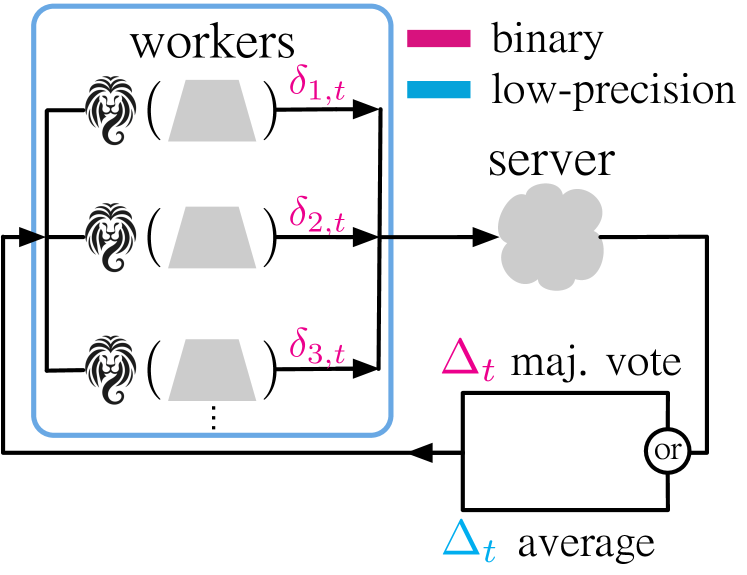
Figure 1: Illustration of Distributed-Lion. Each worker keeps its own optimizer state and applies the Lion optimizer individually to a binary update $\delta_{i,t}=\texttt{Lion}(x,\mathcal{D}_{i})$ (without the weight decay), then the server aggregates all $\delta_{i,t}$ to producea binary $\Delta_{t}$ by majority vote (or a integer $\Delta_{t}$ by averaging) and send it back to all workers. The workers then apply $\Delta_{t}$ and weight decay to update their model parameters. See Algorithm 1 for details.

In this study,we tailor the Lion optimizer for distributed training. The Lion optimizer is particularly suitable for this context due to two main attributes: (1) its simple update mechanism that relies solely on first-order momentum, and (2) its use of the $\mathrm{sign}(\cdot)$ function. We showcase the effective employment of the $\mathrm{sign}(\cdot)$ function to streamline communication processes, leading to the development of a novel distributed training framework named Distributed Lion. Within the Distributed Lion framework, each participating worker independently adjusts the model parameters using a distinct instance of the Lion optimizer, thereby maintaining separate optimizer states. A distinctive feature of this framework is the mode of communication between workers and the central server, which is restricted to binary or low-precision vectors.Crucially, in this setup, workers convey updates rather than raw gradients to the central server. The server, in turn, aggregates these updates through either a straightforward averaging process (Distributed Lion-Avg) or a majority voting mechanism (Distributed Lion-MaVo). In the case of Distributed Lion-MaVo, the consolidated update is maintained as a binary vector, whereas for Distributed Lion-Avg, given the presence of $n$ workers, each element of the update vector is encoded using $\log(n)$ bits. This approach markedly reduces the bandwidth requirements compared to traditional distributed training methods, which typically rely on high-precision floating-point vectors for communication. The bandwidth efficiencies achieved by our method are detailed in Table 1. We summarize our primary contributions as follows:

	Bandwidth Requirement
Method	Worker$\rightarrow$Server	Server$\rightarrow$Worker
Global Lion/AdamW	$32d$	$32d$
TernGrad (Wen et al., 2017)	$1.5d$	$\log(2n+1)d$
DGC (Lin et al., 2017)	$(1-\eta)32d$	$32d$
Distributed Lion-Avg	$d$	$\log(n)d$
Distributed Lion-MaVo	$d$	$d$

Table 1: Minimum bandwidth requirements of different methods for a model with $d$ parameters and $n$ workers. For Deep Gradient Compression (DGC), $\eta$ denotes the compression rate (default: $\eta=0.96$).

• We introduce the Distributed Lion algorithm, a simple yet effective approach to extend Lion to distributed training, where all communications between workers and the server are done through binary or low-precision vectors (Section 3).

• We provide theoretical analysis to ensure the convergence of Distributed Lion (Section 4).

• Empirically, we demonstrate that on both vision and language modeling tasks, Distributed Lion achieves comparable performance against applying Lion and Adam with the synchronized gradients from all workers, while being significantly more communication efficient. In addition, we show that Distributed Lion achieves a better trade-off than existing efficient distributed training methods like deep gradient compression (Lin et al., 2017) and ternary gradients (Wen et al., 2017) (Section 5).

2 Related Work

In this section, we provide a summary of optimizers that use the sign function and existing literature on bandwidth-friendly distributed training.

Sign Operation in Optimization

The sign operation is integral to optimization for several reasons. Primarily, it acts as a normalization mechanism by disregarding the magnitude of gradients, thereby equilibrating updates across different dimensions and potentially facilitating the avoidance of saddle points. Additionally, the binary nature of the sign function’s output significantly reduces the memory footprint required for storing gradient updates. The concept of sign-based optimization dates back to RProp (Riedmiller & Braun, 1993) and has seen renewed interest with the advent of SignSGD and its momentum-enhanced variant, Signum (Bernstein et al., 2018b). A more recent advancement is the generalized SignSGD algorithm introduced by (Crawshaw et al., 2022), which incorporates a preconditioner, making it a superset of SignSGD and akin to Adam in certain aspects. A noteworthy addition to sign-based optimizers is the Lion optimizer, which emerged from evolutionary program search, achieving performance comparable to Adam (Kingma & Ba, 2014) and AdamW (Loshchilov & Hutter, 2017) for the first time. Lion distinguishes itself from Signum by employing a different convex combination for outputting local updates, a technique referred to as the double-$\beta$ scheme, reminiscent of Nesterov’s momentum update, and encapsulates Signum as a particular case. On the theoretical front, SignSGD and Signum have been shown to exhibit convergence rates comparable to traditional SGD (Bernstein et al., 2018b). Recent work by (Sun et al., 2023) has extended the theoretical understanding by providing a convergence theory that relaxes the requirements for bounded stochastic gradients and enlarged batch sizes. Additionally, Lion has demonstrated its capability in performing constrained optimization under the $\ell_{\infty}$-norm constraint (Chen et al., 2023a).

Distributed Training

In addressing the communication constraints of distributed training, the research community has devised several innovative strategies, prominently featuring asynchronous Stochastic Gradient Descent (SGD), gradient quantization, and sparsification techniques. Asynchronous SGD offers a solution by enabling parameter updates immediately after back-propagation, bypassing the need for gradient synchronization, thereby expediting the training process (Chen et al., 2016; Zheng et al., 2017; Liu et al., 2024). Li et al. (2022) utilizes sketch-based algorithms for lossless data compression (Li et al., 2024), achieving an asymptotically optimal compression ratio (Li et al., 2023). However, its applicability is limited to highly sparse gradients, making it orthogonal to our research. In the realm of gradient quantization, methods such as 1-bit SGD (Seide et al., 2014), QSGD (Alistarh et al., 2017), and TernGrad (Wen et al., 2017) are pivotal. These approaches compact the gradient data, substantially reducing the required communication bandwidth, with 1-bit SGD demonstrating a tenfold acceleration in speech applications and both QSGD and TernGrad confirming the feasibility of quantized training in maintaining convergence. Moreover, gradient sparsification further mitigates the communication load by transmitting only the most substantial gradients. Techniques like threshold quantization and Gradient Dropping (Aji & Heafield, 2017) exemplify this, with Gradient Dropping notably achieving a 99 reduction in gradient exchange with minimal impact on performance metrics, such as a mere 0.3 loss in BLEU score for machine translation tasks. The recent Deep Gradient Compression (DGC) strategy (Lin et al., 2017) also contributes to this field by incorporating momentum correction and local gradient clipping among other methods to maintain accuracy while significantly reducing communication demands, albeit at the cost of increased computational overhead. Compared to gradient quantization methods, Distributed Lion uniquely leverages the binary nature of Lion’s update and can be viewed as performing quantization on updates rather than the gradient.

Algorithm 1 Distributed Lion Training

  Inputs: Initial parameters $x_{0}\in\mathbb{R}^{d}$, datasets $\{\mathcal{D}_{1},\dots,\mathcal{D}_{N}\}$, loss function $f$, learning rate $\epsilon$, hyper-parameters $\beta_{1},\beta_{2}\in[0,1]$ (default to $0.9,0.99$), and the weight decay $\lambda$.

  

  Initialization: $t=0$,  $\forall i,m_{i,0}=\bm{0}$, and $x_{i,0}=x_{0}$.

  while not convergent do

     Worker-side: Each worker $i$ samples a batch $\xi_{i,t}\in D_{i}$, computes the following, and sends ${\color[rgb]{1,0,1}\delta_{i,t}}$ to the server:

$$\text{if}\leavevmode\nobreak\ t>0,\leavevmode\nobreak\ \leavevmode\nobreak\ x_{i,t} \leftarrow x_{i,t-1}-\epsilon\big{(}\Delta_{t-1}+\lambda x_{i,t-1}\big{)}$$

$${\color[rgb]{1,0,1}\delta_{i,t}} \leftarrow\mathrm{sign}\big{(}\beta_{1}m_{i,t}+(1-\beta_{1})\nabla_{x}f(x_{i,t};\xi_{i,t})\big{)}$$

$$m_{i,t+1} \leftarrow\beta_{2}m_{i,t}+(1-\beta_{2})\nabla_{x}f(x_{i,t};\xi_{i,t}).$$

     Server-side: The server computes the aggregated update $\Delta_{t}$ and broadcast it to all workers:

$$\Delta_{t}=\begin{cases}{\color[rgb]{0,1,1}\frac{1}{N}\big{(}\sum_{i=1}^{N}\delta_{i,t}\big{)}}&\text{(Averaging)}\\ {\color[rgb]{1,0,1}\mathrm{sign}\big{(}\sum_{i=1}^{N}\delta_{i,t}\big{)}}&\text{(Majority Vote)}\\ \end{cases}\leavevmode\nobreak\ \leavevmode\nobreak\ \leavevmode\nobreak\ \leavevmode\nobreak\ \text{and}\leavevmode\nobreak\ \leavevmode\nobreak\ \leavevmode\nobreak\ \leavevmode\nobreak\ t\leftarrow t+1.$$

  end while

3 The Distributed Lion

We introduce the distributed learning problem and then our Distributed Lion framework.

3.1 Distributed Training

In distributed training, we aim to minimize the following learning objective:

$$\min_{x}F(x)=\frac{1}{N}\sum_{i=1}^{N}\mathbb{E}_{\xi_{i}\sim\mathcal{D}_{i}}\bigg{[}f(x;\xi_{i})\bigg{]}.$$ (2)

Here, $N$ denotes the number of workers, $\{\mathcal{D}_{i}\}$ are $N$ datasets, and $x$ is the model parameter (e.g., the weights of a neural network). In the distributed learning setting, each worker $i\in[n]$ will get its own dataset $\mathcal{D}_{i}$, and we assume there is a centralized server that all workers can communicate with. The simplest distributed training technique is to perform distributed gradient aggregation:

$$g_{\text{server}}=\frac{1}{N}\sum_{i=1}^{N}g_{i},\leavevmode\nobreak\ \leavevmode\nobreak\ \leavevmode\nobreak\ \text{where}\leavevmode\nobreak\ \leavevmode\nobreak\ \leavevmode\nobreak\ g_{i}=\mathbb{E}_{\xi_{i}\sim\mathcal{D}_{i}}\big{[}\nabla_{x}f(x;\xi_{i})\big{]}.$$ (3)

Here, each local gradient $g_{i}$ is an unbiased estimation of the true gradient $\nabla_{x}F(x)$ when $\mathcal{D}_{i}$ are i.i.d. drawn from the same underlying distribution. The server aggregates all local gradients into $g_{\text{server}}$, and then applies an optimizer like Adam (Kingma & Ba, 2014) on top of $g_{\text{server}}$. However,the aggregation step requires communicating the full gradient vectors $g_{i}$,which can be expensive for large models.

Notation.

Given a function $f(x;\xi)$, the gradient $\nabla f(x;\xi)$ is taken with respect to variable $x$. We use $\|\cdot\|$, $\|\cdot\|_{1}$, and $\|\cdot\|_{\infty}$ to denote the $\ell_{2}$, $\ell_{1}$, and $\ell_{\infty}$ norm, respectively. $\xi_{i,t}$ is the sampled data at time $t$ for the $i$-th worker and $g_{i,t}=\nabla f(x_{t};,\xi_{i,t})$. We similarly denote $z_{i,t}$ as any variable $z$ at time $t$ from worker $i$.

3.2 Distributed Lion

The main idea of Distributed Lion is to leverage the binary nature of the Lion’s update for efficient communication. To enable that, we want the workers to only send the binary updates to the server. As a result, we let each worker keep tracks of its own optimizer state, i.e., the momentum $m_{i,t}$. Then at each step, each worker $i$ first computes:

$$\begin{split}m_{i,t+1}=\beta_{2}m_{i,t}+(1-\beta_{2})g_{i,t},\\ {\color[rgb]{1,0,1}\delta_{i,t}}=\mathrm{sign}(\beta_{1}m_{i,t}+(1-\beta_{1})g_{i,t}).\\ \end{split}$$ (4)

Then all workers send the $\delta_{i,t}$ back to the server. The server receives the binary “updates” from all workers and then aggregates them. Here, we propose two simple ways for aggregation. Denote $S_{t}=\sum_{i=1}^{N}\delta_{i,t}$, which is a vector of integers in $\{0,\ldots N\}$. Define the aggregation as follows:

$$\Delta_{t}=\text{aggregate}(S_{t})=\begin{cases}{\color[rgb]{0,1,1}\frac{1}{N}S_{t}}&\text{(Averaging)}\\ {\color[rgb]{1,0,1}\mathrm{sign}(S_{t})}&\text{(Majority Vote)}\\ \end{cases}.$$ (5)

So we simply average or take the majority vote from all $\{\delta_{i,t}\}$. Here, we denote binary vectors in magenta and low precision vectors in cyan. In the end, the server broadcasts $\Delta_{t}$ back to each worker $i$, and each worker performs

$$x_{i,t+1}=x_{i,t}-\epsilon(\Delta_{t}+\lambda x_{i,t}),$$ (6)

where $\epsilon$ is the step size and $\lambda$ is the weight decay coefficient.

Communication Cost

In both variants of Distributed Lion,the $N$ workers only need to send the binaryvectors $\delta_{i,t}$ to the server.The servers need to send the aggregated updates $\Delta_{t}$ back to the workers,which is binary when using the majority vote aggregation, and an integer in $\{0,\ldots,N\}$when using the averaging aggregation.Note that an integer in $\{0,\ldots,N\}$can be represented by at most $\log(N)$ bits.In practice, usually $N\ll 2^{32}$ hence $\log(N)<32$ and we still save the communication bandwidth even with the average aggregation, comparing against communicating with floating point numbers (Check Table 1). The whole Distributed Lion algorithm is summarized in Algorithm 1.

4 Theoretical Analysis

We provide our theoretical analysis of the Distributed Lion algorithm, both with the averaging and the majority vote aggregation methods. In the following, we first describe that the distributed training problem can be viewed as a constrained optimization problem when Distributed Lion is used. We provide convergence results for Distributed Lion with both aggregation methods.

4.1 Lion as Constrained Optimization

Chen et al. (2023a) showed that the (global) Lion is a theoretically novel and principled approach for minimizing a general loss function $f(x)$ while enforcing a box constrained optimization problem:

$$\min_{x\in\mathbb{R}^{d}}f(x)\leavevmode\nobreak\ \leavevmode\nobreak\ \leavevmode\nobreak\ \leavevmode\nobreak\ s.t.\leavevmode\nobreak\ \leavevmode\nobreak\ \leavevmode\nobreak\ \leavevmode\nobreak\ \left\lVert\lambda x\right\rVert_{\infty}\leq 1,$$ (7)

where the constrained is introduceddue to the use of the weight decay coefficient $\lambda$.Moreover, Chen et al. (2023a) showed that the Lion dynamics consists of two phases:1) [Phase 1] Whenthe constraint is not satisfied, that is, $x\not\in\mathcal{F}$, where $\mathcal{F}$ is the feasible set

$$\mathcal{F}\overset{def}{=}\{x\colon\left\lVert\lambda x\right\rVert_{\infty}\leq 1\},$$ (8)

it exponentially decays the distance to $\mathcal{F}$:there exists an $\alpha\in(0,1)$, such that

$$\mathrm{dist}(x_{t+n},\mathcal{F})\leq\alpha^{n}\mathrm{dist}(x_{t},\mathcal{F}).$$

where $n\geq 0$.Hence, $x_{t}$ converges to $\mathcal{F}$ rapidly and stays within $\mathcal{F}$ once it arrived it.2) [Phase 2]After $\lambda x_{t}$ enters $\mathcal{F}$, the dynamics minimizes the objective $f(x)$ while being confined within the set $\mathcal{F}$.This step is proved in Chen et al. (2023a)by constructing a Lyapunov function when $\mathrm{sign}(\cdot)$is treated as the sub-gradient of a convex function.

4.2 Convergence Analysis

In this section,we analyze the convergence of distributed Lion algorithms.Similar to the case of global Lion,we show that distributed Lion also solves the box constrained optimization (7).Its dynamics also unfolds into two phasesaligning with Lion’s dynamics: Phase I shows rapid convergence to a feasible set $\mathcal{F}$, while Phase II seeks to minize the objective $f(x)$ within the feasible set $\mathcal{F}$.Different from the Lyapunov approach used in Chen et al. (2023a),the proof of our Phase II resultis made by introducinga surrogate metric $\mathcal{S}(x)$ of constrained optimality, and providing upper bound of $\mathcal{S}(x_{t})$ following the algorithm.Our analysis makes the following assumptions.

Assumption 4.1 (Variance bound).

$\mathcal{D}_{i}$ is i.i.d. drawn from a common distribution $\mathcal{\pi}_{*}$, and the stochastic sample $\xi^{i}\sim\mathcal{D}_{i}$ is i.i.d. and upon receiving query $x\in\mathbb{R}^{d}$, the stochastic gradient oracle gives us an independent unbiased estimate $\nabla f(x;\xi^{i})$ from the $i$-th worker that has coordinate bounded variance:

$$\mathbb{E}_{\xi}[\nabla f(x;\xi^{i})]=\nabla f(x),$$

$$\mathbb{E}_{\xi}\left[\|\nabla f(x;\xi^{i})-\nabla f(x)\|^{2}\right]\leq\sigma^{2}.$$

Assumption 4.2 (Smooth and Differentiable $f$).

Function $f(\cdot)$ is differentiable and L-smooth.

Assumption 4.3 (Bias Correction).

Consider the sequence $\{m_{t}^{i}\}_{t>0,i\in[N]}$ generated by Algorithm 1, $\mathbb{E}[\tilde{m}_{t}^{i}]/\mathbb{E}[\mathrm{sign}(\tilde{m}_{t}^{i})]\geq 0$.

Note that assumption 4.2 4.1 are standard in the analysis of stochastic optimization algorithms (Bottou et al., 2018; Sun et al., 2023).When Assumption 4.1 holds, $\mathbb{E}\|\frac{1}{N}\sum_{i=1}^{N}\nabla f(x;\xi_{i})-\nabla f(x)\|^{2}\leq\sigma^{2}/N$.In distributed training setting, $m_{1,t},m_{2,t},\cdots,m_{N,t}$ are i.i.d., so $\mathbb{E}[\beta_{1}m_{i,t}+(1-\beta_{1})g_{i,t}]$ and $\mathbb{E}[\mathrm{sign}(\tilde{m}_{t+1}^{i})]$ don’t depend on $i$. Assumption 4.3 evaluates the discrepancy between the expected value and the expected sign of a measure, positing that the expected values of $\tilde{m}_{t}^{i}$ and $\tilde{\mathrm{sign}}(m_{t}^{i})$ ought to share the same sign.We now present our results.Similar to the case of global Lion,the dynamics of distributed lion can also be divided into two phasesdepending on if the constraint $x\in\mathcal{F}$ is satisfied.

Phase I ($x\not\in\mathcal{F}$)

In line with the behavior observed in the global Lion model,when the constraint is not satisfied,both variants of distributed Lion decrease the distance to the feasible set exponentially fast.

Theorem 4.4 (Phase I).

Assume $f\colon\mathbb{R}^{d}\to\mathbb{R}$ is $L$-smooth, $\beta_{1},\beta_{2}\in(0,1)$, and $\beta_{2}>\beta_{1}$, and $\epsilon,\lambda>0$. Let $(x_{t})_{t\geq 0}$ be generated by Algorithm 1.Define $\mathcal{F}=\{x\colon\left\lVert\lambda x\right\rVert_{\infty}\leq 1\}$, and $\mathrm{dist}(x_{t},\mathcal{F})=\inf_{z\in\mathcal{F}}\left\lVert z-x_{t}\right\rVert$ w.r.t. any norm $\left\lVert\cdot\right\rVert$.For any two non-negative integers $s\leq t$, then $\forall s\leq t$, we have

$$\mathrm{dist}(x_{t},\mathcal{F})\leq(1-\epsilon\lambda)^{t-s}\mathrm{dist}(x_{s},\mathcal{F}).$$

Hence, $x_{t}$ converges to $\mathcal{F}$ rapidly and stays within $\mathcal{F}$ once it arrived.

Phase II ($x\in\mathcal{F}$)

Now, we present the main result of the analysis for Phase II in Theorems 4.6, 4.7, and 4.8.We start with introducing a surrogate metricthat quantifies the optimality of the solution within Phase II:

$$\mathcal{S}(x):=\langle\nabla f(x),\mathrm{sign}(\nabla f(x))+\lambda x\rangle.$$ (9)

Let’s delve into the implications of $\mathcal{S}(x)=0$.

Proposition 4.5.

Assume $f$ is continuously differentiable, $\lambda>0$, and $\left\lVert\lambda x\right\rVert_{\infty}\leq 1$.Then $\mathcal{S}(x)=0$ implies a KKT stationary condition of $\min_{x}f(x)\leavevmode\nobreak\ s.t.\leavevmode\nobreak\ \left\lVert\lambda x\right\rVert_{\infty}\leq 1$.

This KKT score (9) is tailored to encompass the stationary solutions of the box-constrained problem as described in (7). Building on this, we then proceed to analyze the convergence for the majority vote, averaging, and global LION strategies throughout this section.

Theorem 4.6 (Majority Vote).

Assumptions 4.1, 4.2, and 4.3 hold, consider the Majority vote scheme in Algorithm 1, $\beta_{1},\beta_{2}\in(0,1)$, and $\beta_{2}>\beta_{1}$, and $\sigma\leq 2\sqrt{d}\beta_{1}\beta_{2}^{t}\|\nabla f(x_{0})\|,1\leq t\leq T$ , and $\epsilon,\lambda>0$. Let $(x_{t})_{t\geq 0}$ be generated by Majority Vote, and it is in Phase II: $\|\lambda x_{t}\|_{\infty}\leq 1$ for all $t$.We have

$$\frac{1}{T}\sum_{t=1}^{T}\mathbb{E}\mathcal{S}(x_{t})\leq\frac{f(x_{0})-f^{*}}{T\epsilon}+\frac{2D\beta_{1}\beta_{2}\sqrt{d}\|\nabla f(x_{0})\|}{T(1-\beta_{2})}$$

$$+\frac{4\beta_{1}L\epsilon d}{1-\beta_{2}}+\frac{2\sqrt{d}\sigma(1+\sqrt{C})+2\rho}{\sqrt{N}}+2L\epsilon d,$$

where $C=\beta_{1}^{2}(1-\beta_{2})\frac{1}{1+\beta_{2}}+(1-\beta_{1})^{2}$, $D=\max\{1,\sigma/\left(2\sqrt{d}\beta_{1}\beta_{2}^{T}\|\nabla f(x_{0})\|\right)\}$,

$$\rho_{t}[k]=\begin{cases}0\leavevmode\nobreak\ \leavevmode\nobreak\ \leavevmode\nobreak\ \leavevmode\nobreak\ \leavevmode\nobreak\ \leavevmode\nobreak\ \leavevmode\nobreak\ \leavevmode\nobreak\ \leavevmode\nobreak\ \leavevmode\nobreak\ \leavevmode\nobreak\ \leavevmode\nobreak\ \leavevmode\nobreak\ \leavevmode\nobreak\ \leavevmode\nobreak\ \leavevmode\nobreak\ \leavevmode\nobreak\ \leavevmode\nobreak\ \leavevmode\nobreak\ \leavevmode\nobreak\ \leavevmode\nobreak\ \leavevmode\nobreak\ \leavevmode\nobreak\ \leavevmode\nobreak\ \text{if\leavevmode\nobreak\ $\mathbb{E}[\mathrm{sign}(\tilde{m}_{t+1}^{i}[k])]=0$,}\\ \mathbb{E}[\tilde{m}_{t+1}^{i}[k]]/\mathbb{E}[\mathrm{sign}(\tilde{m}_{t+1}^{i}[k])]\leavevmode\nobreak\ \leavevmode\nobreak\ \leavevmode\nobreak\ \leavevmode\nobreak\ \leavevmode\nobreak\ \leavevmode\nobreak\ \leavevmode\nobreak\ \leavevmode\nobreak\ \leavevmode\nobreak\ \leavevmode\nobreak\ \text{else,}\end{cases}$$

, and $\rho=\max_{1\leq t\leq T}\left\lVert\rho_{t}\right\rVert$.

The result above shows that $\frac{1}{T}\sum_{t=1}^{T}\mathbb{E}\mathcal{S}(x_{t})$ decays with an $\mathcal{O}(\frac{1}{T\epsilon}+\frac{1}{T(1-\beta_{2})}+\epsilon+\frac{1}{\sqrt{N}})$.This rate is in fact on par with global Lion as we show in the following result:

Theorem 4.7 (Global).

Assumptions 4.1 and 4.2 hold, Consider the scheme in Algorithm (15), with the same settings in Theorem 4.6,we have

$$\frac{1}{T}\sum_{t=1}^{T}\mathbb{E}\mathcal{S}(x_{t}) \leq\frac{f(x_{0})-f^{*}}{T\epsilon}+\frac{2\beta_{1}\beta_{2}\sqrt{d}\|\nabla f(x_{0})\|}{T(1-\beta_{2})}$$

$$+\frac{4\beta_{1}L\epsilon d}{1-\beta_{2}}+\frac{2(1-\beta_{1})\sqrt{d}\sigma}{\sqrt{N}}+2L\epsilon d.$$

Theorem 4.8 (Averaging).

Assumptions 4.1 and 4.2 hold, consider the Averaging scheme in Algorithm 1, with the same settings in Theorem 4.6,we have

$$\frac{1}{T}\sum_{t=1}^{T} \mathbb{E}\mathcal{S}(x_{t})\leq\frac{f(x_{0})-f^{*}}{T\epsilon}+\frac{2\beta_{1}\beta_{2}\sqrt{d}\|\nabla f(x_{0})\|}{T(1-\beta_{2})}$$

$$+\frac{4\beta_{1}L\epsilon d}{1-\beta_{2}}+\frac{2\beta_{1}\sqrt{d}\sigma}{\sqrt{1+\beta_{2}}}+2(1-\beta_{1})\sqrt{d}\sigma+2L\epsilon d$$

The Averaging method’s convergence bound doesn’t improve with more workers since $\frac{1}{N}\sum_{i=1}^{N}\mathrm{sign}(\delta_{i,t})$ doesn’t approximate $\mathrm{sign}(\sum_{i=1}^{N}\delta_{i,t})$ effectively, unlike the Majority Vote’s approach $\mathrm{sign}(\sum_{i=1}^{N}\mathrm{sign}(\delta_{i,t}))$.

5 Experiment

In this section, we perform a thorough evaluation of the Distributed Lion algorithm, employing both the averaging and majority vote aggregation methods. The design of our experiments is aimed at addressing the following questions to ascertain the algorithm’s efficacy and performance:

• (Q1) How does Distributed Lion stand in comparison to global distributed training approaches, i.e., methods that aggregate gradients from local workers and employ an optimizer on the collective gradient?

• (Q2) How does Distributed Lion perform when compared to established communication-efficient distributed training methodologies?

• (Q3) How does Distributed Lion scale on large vision or language problems?

Figure 2: Performance of Distributed Lion v.s. other efficient distributed optimizers on CIFAR-10 with 4, 8, 16, and 32 workers, each worker at each iteration runs on a local batch with size 32. All results are averaged over three seeds.

5.1 Comparing Distributed Lion Against Established Methods on CIFAR-10

To address Q1 and Q2, we compare Distributed Lion with both the averaging and the majority vote methods, against established low-bandwidth distributed training techniques and the global distributed training methods. We consider the following baseline methods: 1) Global AdamW (G-AdamW), where we apply AdamW with the averaged gradients from all workers. 2) Global Lion (G-Lion), where we apply Lion with the averaged gradients from all workers. Note that Global AdamW and Global Lion serve as the performance and communication upper bounds. 3) Distributed Lion with Averaged Updates (D-Lion (Avg)), In contrast to the majority vote mechanism used in Distributed Lion, this variant averages the binary update vectors from all workers. While D-Lion (Avg) might offer improved performance in principle, it comes at the cost of non-binary communication from the server to the workers. 4) TernGrad (Wen et al., 2017). The main idea is to tenarize the gradient into a vector of $\{-1,0,1\}$, which is similar to what Lion does. But this process is done on the gradient level instead of on the update level 5) Gradient Dropping (GradDrop) (Aji & Heafield, 2017). The main idea is to drop insignificant gradient entries and only transmit sparse gradient signals. 6) Deep Gradient Compression (DGC) (Lin et al., 2017). DGC is built on top of the GradDrop, but additionally applies momentum correction, local gradient clipping, momentum factor masking, and warm-up training.

Experiment Setup

For GradDrop, DGC, and TernGrad, we choose the compression rate of $0.04$ (note that $1/32=0.03125$) to match the bandwidth of the D-Lion (MaVo). We conduct experiments on the CIFAR-10 dataset using a vision transformer (ViT) with 6 layers, 8 heads, and a hidden dimension of 512. This is because ViT has arguably become the most widely used architecture in computer vision, and we empirically found no additional gain in performance when using a larger ViT on CIFAR-10. In addition, to validate how Distributed Lion performs with different numbers of workers, we consider $k\in\{4,8,16,32\}$, each worker at each iteration will sample an i.i.d data batch of size 32.We list the optimal hyperparameters selected for each method from Figure 2 in Table 2. The learning rates are selected from $\{0.00005,0.001,0.005,0.01\}$ and the weight decays are selected from $\{0.0005,0.001,0.005\}$. For each experiment, we use a cosine learning rate scheduler and run for 200 epochs, and we ensure that in each epoch, each local worker sees the entire dataset once.

Method	lr $\epsilon$	wd $\lambda$	compression rate
G-AdamW	0.0001	0.0005	-
G-Lion	0.00005	0.005	-
DGC	0.01	0.0005	0.96
GradDrop	0.001	0.0005	0.96
TernGrad	0.001	0.0005	-
D-Lion (Avg)	0.00005	0.005	-
D-Lion (MaVo)	0.00005	0.005	-

Table 2: Hyperparameters for each method in Figure 2. Where lr represents learning rate and wd represents weight decay.

Each experiments are conducted with three random seeds $\{42,52,62\}$, which results in a total of $4\times 7\times 3=84$ experiments.

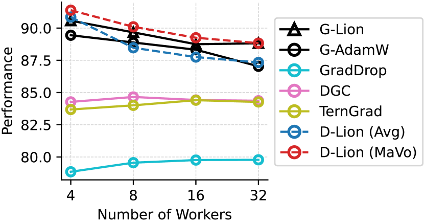
Figure 3: Performance of different methods v.s. $k$.

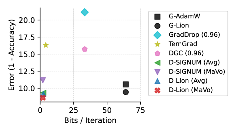
Figure 4: Test Error v.s. Communication Bits per Iteration (closer to the lower-left is better). Note that we set G-Lion and G-AdamW are both 64, because they require 32 bits per parameter, and there are both worker-to-server and server-to-worker communications.

Observation We plot the testing accuracy (Test Acc.) over epochs for different methods in Figure 2, the best testing accuracy of different methods over the number of workers in Figure 3, and the performance versus per-iteration bandwidth in Figure 4 when using $k=4$ workers. From the above plots, we make the following observations.

• Compared to global distributed training methods, D-Lion (MaVo) performs on par with G-Lion. D-Lion (Avg) performs slightly worse than G-Lion but is on par with G-Adamw (Figure 2).

• Compared to established communication efficient distributed training methods, both D-Lion (MaVo) and D-Lion (Avg) outperform GradDrop, DGC and TernGrad by a large margin (Figure 2).

• We observe that both D-Lion (MaVo) and D-Lion (Avg) exhibit strong performance while being 30x more communication efficient than global distributed training methods like G-AdamW. To broaden our comparison, we introduced two additional baseline methods: D-SIGNUM (Avg) and D-SIGNUM (MaVo). These baselines apply our proposed techniques to the SIGNUM framework instead of Lion. We set $\beta=0.99$ for D-SIGNUM. According to our results, depicted in Figure 4, these SIGNUM-based methods do not perform as well as their Lion-based counterparts.

• We notice that the overall performance of the same optimizer becomes worse as $k$ goes larger, this is consistent with the observation made in DGC (Lin et al., 2017). We hypothesize that this may be due to the larger effective batch size resulting in smaller stochasticity, which is consistent with why D-Lion (MaVo) performs a bit better than G-Lion on CIFAR-10 (Figure 3).

Method	Image Classification		Language Modeling
	ViT-S/16	ViT-B/16	GPT-2++ (350M)	GPT-2++ (760M)
AdamW	79.74	80.94	18.43	14.70
G-Lion	79.82	80.99	18.35	14.66
D-Lion (MaVo)	79.69	80.79	18.37	14.66
D-Lion (Avg)	80.11	81.13	18.39	14.69

Table 3: Results on ImageNet classification and OpenWebText language modeling. For ImageNet experiments, we report the Top-1 accuracy. For language modeling experiments, we report the validation perplexity. The best performance is marked with bold text, and the second best with an underline.

Method	Arc-Easy	Arc-Challenge	BoolQ	PIQA	SIQA	HellaSwag	OBQA
0-Shot	76.64	43.06	76.43	78.64	45.96	56.87	33.53
G-AdamW	77.06	46.06	77.23	79.18	48.97	59.23	35.51
G-Lion	77.11	45.54	77.50	79.18	49.64	58.93	35.51
D-Lion (MaVo)	76.86	45.72	77.14	78.92	49.75	58.96	35.71
D-Lion (Avg)	76.35	45.54	76.90	78.76	48.06	59.06	32.14

Table 4: 3-Shot instruction finetuning downstream evaluation results on various datasets. We mark the best performance with bold text and the second one with an underline.

5.2 Scale to Larger Models on Larger Datasets

To answer Q3, we validate Distributed Lion on several large-scale setups including both vision and natural language processing tasks. Under this setting, we compare D-Lion (MaVo) and D-Lion (Avg) against G-AdamW and G-Lion. For the vision task, we tested ViT-S/16 (Dosovitskiy et al., 2020) and ViT-B/16 on the ImageNet-1K (Russakovsky et al., 2015) classification benchmark. For the natural language processing task, we perform both language pretraining and finetuning tasks. This is because Lion has shown good results on language modeling. For the language model pretraining task, we pretrain GPT2++ (Radford et al., 2019) (the GPT-2 model with modern training techniques adopted from the LLaMA model (Touvron et al., 2023)) on the OpenWebText (Gokaslan & Cohen, 2019) benchmark, for both 350M and 760M size models. For the language model finetuning task, we conduct few-shot finetuning of the LLaMA 7B model (Touvron et al., 2023) and evaluate the models’ downstream performance on standard downstream evaluation benchmarks (Clark et al., 2018; Zellers et al., 2019; Clark et al., 2019; Mihaylov et al., 2018; Bisk et al., 2020; Sap et al., 2019).

Experiment Setup

For the ImageNet-1K benchmark, we train all methods for 300 epochs, using a global batch size of 4096 and data augmentations MixUp (Zhang et al., 2017) of 0.5 and AutoAug (Cubuk et al., 2018). When training ViT-S/16, we use a learning rate of $3e^{-3}$ for G-AdamW, with betas of $(0.9,0.999)$ and a weight decay of 0.1. For G-Lion, D-Lion (MaVo), and D-Lion (Avg), we use a learning rate of $3e^{-4}$, betas of $(0.9,0.99)$, and a weight decay of 1.0. As for ViT-B/16, we use a learning rate of $1e^{-3}$ for G-AdamW, with betas of $(0.9,0.999)$ and a weight decay of 1.0, while for all Lion variants, we use a learning rate of $1e^{-4}$, betas of $(0.9,0.99)$, and a weight decay of 10.0.For pretraining language models on the OpenWebText dataset, we build GPT2++ models using the original GPT2 model, but with modern training techniques from the LLaMA model, including using the Gated Linear Unit activation for the multilayer layer perceptron layers (MLPs) and the RMSNorm (Zhang & Sennrich, 2019) instead of the LayerNorm (Ba et al., 2016). Following the Chinchilla scaling law (Hoffmann et al., 2022), we trained the 350M model for 14,000 iterations and the 760M model for 30,000 iterations, both with 1,024 tokens. For G-AdamW, we use a learning rate of $3e^{-4}$, betas of $(0.95,0.99)$, and a weight decay of 0.1. For all Lion variants, we use a learning rate of $9e^{-5}$, betas of $(0.9,0.99)$, and a weight decay of 1.0. All the models are trained under a global batch size of 480. For the instruction finetuning task, we instruct finetune a LLaMA 7B model for 3 epochs with batch size 32. We use $2e^{-5}$ learning rate, betas of $(0.9,0.999)$, 0 weight decay for G-AdamW and $6e^{-6}$, $(0.9,0.99)$ betas, $0.01$ weight decay for all Lion variants. For all pretraining experiments, we use $4\text{nodes}\times 8\text{gpus}=32$ workers. For instruction finetuning experiments, we use 4 workers per experiment.Observation We summarize the results in Table 3 (ImageNet 1K and OpenWebText Language Model Pretraining) and Table 4 (Instruction Finetuning). From these two tables, it is evident that both D-Lion (Avg) and D-Lion (MaVo) can maintain a performance similar to, or even better than, that of G-AdamW and G-Lion, on both large-scale vision and language tasks. We observe that D-Lion (Avg) outperforms D-Lion (MaVo) on ImageNet, and observe the opposite on language modeling and instruction finetuning. We hypothesize that these differences are due to the impact of global batch size. As a result, we recommend using D-Lion (Avg) / (MaVo) when the global batch size is large / small.

6 Conclusion and Future Work

In this paper, we introduced Distributed Lion, a communication-efficient distributed training strategy that builds upon the Lion optimizer’s binary update mechanism. Distributed Lion is designed to minimize communication overhead by allowing workers to independently manage their optimizer states and exchange only binary or low-precision update vectors with the server. We proposed two aggregation techniques within the Distributed Lion framework: average-based (Distributed Lion Avg) and majority vote-based (Distributed Lion MaVo) algorithms. We provide both theoretical and empirical results to demonstrate Distributed Lion’s effectiveness, scalability, and efficiency. Notably, we show that Distributed Lion performs significantly better than existing communication-friendly methods. In the meantime, Distributed Lion demonstrates performance on par with strong global distributed training baselines, while being 32x more communication efficient. As our method is orthogonal to existing communication-efficient methods, an interesting future direction is to combine both techniques from both worlds for further improvement. As a limitation, currently Distributed Lion (Avg / MaVo) performs inconsistently across different datasets and benchmarks, it will be an interesting future research direction to understand when and why one performs better than the other.

7 Broader Impact

This paper presents a novel method that aims to improve distributed training. While we acknowledge that our work could have a multitude of potential societal consequences, we do not believe any specific ones need to be highlighted.

Appendix A Appendix I

This section is focusing on the proof of Lion dynamics, and will be organized into these folders:

• Phase I:

  • Constraint enforcing: Discrete time

• Phase II:

  • Majority Voting convergence

  • Avg update convergence

  • Global LION convergence

In line with the behavior observed in the global Lion approach, Lion under a distributed setting also exhibits the two phases. In Section A.1, we show that converging to box can be exponentially fast using our Algorithm 1. We start with introducing a notion of KKT score function that quantifies a stationary solution to the box constrained optimization problem (7) in Section A.2.Building on this, we then proceed to analyze the convergence in terms of the KKT score function for the majority vote (Section A.2.1), averaging (Section A.2.2), and global LION strategies (Section A.2.3).

A.1 Phase I: Constraint Enforcing

We study phase I in this section. We show that when the constraint is not satisfied,both variants of distributed Lion decrease the distance to the feasible set exponentially fast.

Theorem A.1 (Phase I).

Assume$f\colon\mathbb{R}^{d}\to\mathbb{R}$ is $L$-smooth, $\beta_{1},\beta_{2}\in(0,1)$, and $\beta_{2}>\beta_{1}$, and $\epsilon,\lambda>0$, and $1-\epsilon\lambda\in(0,1)$. Let $(x_{t})_{t\geq 0}$ be generated by Algorithm 1. Define $\mathcal{F}=\{x\colon\left\lVert\lambda x\right\rVert_{\infty}\leq 1\}$, and $\mathrm{dist}(x_{t},\mathcal{F})=\inf_{z\in\mathcal{F}}\left\lVert z-x_{t}\right\rVert$ w.r.t. any norm $\left\lVert\cdot\right\rVert$.For any two non-negative integers $s\leq t$, then $\forall s\leq t$, we have

$$\mathrm{dist}(x_{t},\mathcal{F})\leq(1-\epsilon\lambda)^{t-s}\mathrm{dist}(x_{s},\mathcal{F}).$$

Proof.

Recall Algorithm 1:

$$\delta_{i,t} \leftarrow\mathrm{sign}\big{(}\beta_{1}m_{i,t}+(1-\beta_{1})\nabla_{x}f(x_{t};\xi_{i,t})\big{)}$$

$$m_{i,t+1} \leftarrow\beta_{2}m_{i,t}+(1-\beta_{2})\nabla_{x}f(x_{t};\xi_{i,t})$$

$$\Delta_{t} =\begin{cases}\frac{1}{N}\big{(}\sum_{i=1}^{N}\delta_{i,t}\big{)}&\text{(Averaging)}\\ \mathrm{sign}\big{(}\sum_{i=1}^{N}\delta_{i,t}\big{)}&\text{(Majority Vote)}\\ \end{cases}$$

$$x_{t+1} =x_{t}-\epsilon(\Delta_{t}+\lambda x_{t})$$

Rewrite the update into the following form:

$$x_{t+1}=(1-\epsilon\lambda)x_{t}-\epsilon\Delta_{t},$$

Define $w_{s\to t}=(1-\epsilon\lambda)^{t-s}$.Unrolling this update yields,

$$x_{t} =(1-w_{s\to t})z_{s\to t}+w_{s\to t}x_{s},\leavevmode\nobreak\ \leavevmode\nobreak\ \leavevmode\nobreak\ \leavevmode\nobreak\ \leavevmode\nobreak\ \leavevmode\nobreak\ \leavevmode\nobreak\ \leavevmode\nobreak\ \leavevmode\nobreak\ \leavevmode\nobreak\ z_{s\to t}=\frac{\sum_{k=s}^{t-1}w_{k\to t}(-\Delta_{t}/\lambda)}{\sum_{k=s}^{t-1}w_{k\to t}}.$$

We have $z_{s\to t}\in\mathcal{F}$ since $-\Delta_{t}/\lambda\in\mathcal{F}$. For any $\epsilon>0$, let $\hat{x}_{s}\in\mathcal{F}$ be the point satisfying $\left\lVert\hat{x}_{s}-x_{s}\right\rVert\leq\mathrm{dist}(x_{s},\mathcal{F})+\eta$.Hence, we have

$$\mathrm{dist}(x_{t},\leavevmode\nobreak\ \mathcal{F}) =\inf_{z\in\mathcal{F}}\left\lVert x_{t}-z\right\rVert$$

$$\leq\left\lVert x_{t}-(1-w_{s\to t})z_{s\to t}-w_{s\to t}\hat{x}_{s})\right\rVert$$

$$=w_{s\to t}\left\lVert x_{s}-\hat{x}_{s}\right\rVert$$

$$\leq(1-\epsilon\lambda)^{t-s}(\mathrm{dist}(x_{s},\mathcal{F})+\eta).$$

As $\eta\to 0$, we achieve the desired result.∎

A.2 Phase II

We study the convergence of Phase II in this section. We begin by defining a KKT score function to quantify stationary solutions for the box-constrained optimization problem discussed in Section A.2. Following this, we analyze convergence through the KKT score across majority vote (Section A.2.1), averaging (Section A.2.2), and global Lion strategies (Section A.2.3).First, we list the following assumptions used in our proof.

Assumption A.2 (Smooth and Differentiable $f$).

Function $f(\cdot)$ is differentiable and L-smooth.

Assumption A.3 (Variance bound).

$\mathcal{D}_{i}$ is i.i.d. drawn from a common distribtion $\mathcal{\pi}_{*}$, and the stochastic sample $\xi^{i}\sim\mathcal{D}_{i}$ is i.i.d. and upon receiving query $x\in\mathbb{R}^{d}$, the stochastic gradient oracle gives us an independent unbiased estimate $\nabla f(x;\xi^{i})$ from the $i$-th worker that has coordinate bounded variance:

$$\mathbb{E}_{\xi}[\nabla f(x;\xi^{i})]=\nabla f(x),\qquad\mathbb{E}_{\xi}\left[\|\nabla f(x;\xi^{i})-\nabla f(x)\|^{2}\right]\leq\sigma^{2}.$$

Assumption A.4 (Bias Correction).

Consider the sequence $\{m_{t}^{i}\}_{t>0,i\in[N]}$ generated by Algorithm 1, $\mathbb{E}[\tilde{m}_{t}^{i}]/\mathbb{E}[\mathrm{sign}(\tilde{m}_{t}^{i})]\geq 0$.

Here we define the a KKT score function for box constrained problem (7):

$$\mathcal{S}(x):=\langle\nabla f(x),\mathrm{sign}(\nabla f(x))+\lambda x\rangle.$$

Proposition A.5.

Assume $f$ is continuously differentiable, $\lambda>0$, and $\left\lVert\lambda x\right\rVert_{\infty}\leq 1$.Then $\mathcal{S}(x)=0$ implies a KKT stationary condition of $\min_{x}f(x)\leavevmode\nobreak\ s.t.\leavevmode\nobreak\ \left\lVert\lambda x\right\rVert_{\infty}\leq 1$.

Proof.

We will verify that $\mathcal{S}(x)=0$ coincides with the first order KKT conditions of the box constrained optimization problem (7).Recall the box constrained problem in (7), we can rewrite it into the following formulation:

$$\min_{x\in\mathbb{R}^{d}}f(x)\leavevmode\nobreak\ \leavevmode\nobreak\ \leavevmode\nobreak\ \leavevmode\nobreak\ s.t.\leavevmode\nobreak\ \leavevmode\nobreak\ \leavevmode\nobreak\ \leavevmode\nobreak\ \lambda x_{i}-1\leq 0,\leavevmode\nobreak\ \leavevmode\nobreak\ \leavevmode\nobreak\ -\lambda x_{i}-1\leq 0,\leavevmode\nobreak\ \leavevmode\nobreak\ \leavevmode\nobreak\ \forall\leavevmode\nobreak\ i\in[d].$$

Let $\mu=(\mu_{1},\mu_{2},\cdots,\mu_{d})^{\top}$ and $\tilde{\mu}=(\tilde{\mu}_{1},\tilde{\mu}_{2},\cdots,\tilde{\mu}_{d})^{\top}$, then its first order KKT stationary condition can be written as:

$$\partial_{x_{i}}f(x)+\mu_{i}\lambda-\tilde{\mu}_{i}\lambda=0$$ //Stationarity

$$\mu_{i}(\lambda x_{i}-1)=0,\leavevmode\nobreak\ \leavevmode\nobreak\ \leavevmode\nobreak\ \tilde{\mu}_{i}(-\lambda x_{i}-1)=0$$ //Complementary slackness

$$\mu_{i}\geq 0,\leavevmode\nobreak\ \leavevmode\nobreak\ \leavevmode\nobreak\ \tilde{\mu}_{i}\geq 0$$ //Dual feasibility

$$\lambda x_{i}-1\leq 0,\leavevmode\nobreak\ \leavevmode\nobreak\ \leavevmode\nobreak\ -\lambda x_{i}-1\leq 0$$ //Primal feasibility

$$\forall\leavevmode\nobreak\ i\in\{1,2,\cdots,d\}.$$

Expressing $\mathcal{S}(x)$ element-wisely, we obtain:

$$\mathcal{S}(x)=\sum_{k=1}^{d}\mathcal{S}_{k}(x), \mathcal{S}_{k}(x)=\partial_{x_{k}}f(x)\cdot\left(\mathrm{sign}(\partial_{x_{k}}f(x))+\lambda x_{k}\right),$$ with

where $x_{k}$ denotes the $k$-th element of vector $x$.Since $\left\lVert\lambda x\right\rVert_{\infty}\leq 1$, we have $\mathcal{S}_{k}(x)\geq 0$, because

$$\mathcal{S}_{k}(x) =\partial_{x_{k}}f(x)\cdot\left(\mathrm{sign}(\partial_{x_{k}}f(x))+\lambda x_{k}\right)$$

$$=|\partial_{x_{k}}f(x)|+\lambda\partial_{x_{k}}f(x)\cdot x_{k}$$

$$\geq|\partial_{x_{k}}f(x)|-|\partial_{x_{k}}f(x)|\cdot|\lambda x_{k}|$$

$$=|\partial_{x_{k}}f(x)|(1-|\lambda x_{k}|)$$

$$\geq 0\leavevmode\nobreak\ \leavevmode\nobreak\ \leavevmode\nobreak\ \leavevmode\nobreak\ \leavevmode\nobreak\ \leavevmode\nobreak\ \leavevmode\nobreak\ \text{{\color[rgb]{1,0,1}//since $\left\lVert\lambda x\right\rVert_{\infty}\leq 1.$}}$$

Hence, if $\mathcal{S}(x)=0$, we have $\mathcal{S}_{k}(x)=0$for each component $k$. It means that we have either $\mathrm{sign}(\partial_{x_{k}}f(x))+\lambda x_{k}=0$ or $\partial_{x_{k}}f(x)=0$ for each coordinate $k$.There are two primary cases to consider for each $k$:

• Case I: $\partial_{x_{k}}f(x)=0$. This suggests that we reach a stationary condition of $f(x)$ w.r.t. coordinate $x_{k}$, and the KKT condition is satisfied in this case with $\mu_{k}=\tilde{\mu}_{k}=0$.

• Case II: $\mathrm{sign}(\partial_{x_{k}}f(x))+\lambda x_{k}=0$, it follows that $x_{k}=-\frac{1}{\lambda}\mathrm{sign}(\partial_{x_{k}}f(x))$.

  • if $\mathrm{sign}(\partial_{x_{k}}f(x)=1$, then $\partial_{x_{k}}f(x)\geq 0$, and the KKT condition is satisfied with $\mu_{k}=0$ and $\tilde{\mu}_{k}=\partial_{x_{k}}f(x)/\lambda$

  • if $\mathrm{sign}(\partial_{x_{k}}f(x))=-1$, then $\partial_{x_{k}}f(x)\leq 0$, and the KKT condition is satisfied with $\tilde{\mu}_{k}=0$ and $\mu_{k}=\partial_{x_{k}}f(x)/\lambda$.

It turns out the two cases above exactly covers the KKT stationary solution pair $(x,\mu,\tilde{\mu})$ of the box constrained problem in (7).In conclusion, $\mathcal{S}(x)=0$ signifies reaching a stationary point of the bound-constrained optimization problem, as formulated in (7), providing critical insights into the convergence behavior of the algorithm under consideration.∎

A.2.1 Majority Vote

Assume $f\colon\mathbb{R}^{d}\to\mathbb{R}$ is $L$-smooth, and $N$ is the number of workers, on the $i$-th worker,consider the following scheme based on the majority vote:

$$\begin{split}&g_{t}^{i}:=\nabla f(x_{t};\xi_{t}^{i})\\ &m_{t+1}^{i}=\beta_{2}m_{t}^{i}+(1-\beta_{2})g^{i}_{t}\\ &{\tilde{m}}_{t+1}^{i}=\beta_{1}m_{t}^{i}+(1-\beta_{1})g^{i}_{t}\\ &x_{t+1}=x_{t}-\epsilon\left(\mathrm{sign}\left(\sum_{i=1}^{N}\mathrm{sign}(\tilde{m}^{i}_{t+1})\right)+\lambda x_{t}\right).\leavevmode\nobreak\ \leavevmode\nobreak\ \leavevmode\nobreak\ \leavevmode\nobreak\ \leavevmode\nobreak\ \leavevmode\nobreak\ \leavevmode\nobreak\ \text{{\color[rgb]{1,0,1}//Majority Voting}}\end{split}$$ (10)

Theorem A.6 (Convergence in Phase II).

Assumption A.2 A.3 A.4 hold, consider the scheme in Algorithm 10, and $\beta_{1},\beta_{2}\in(0,1)$, and $\beta_{2}>\beta_{1}$, and $\epsilon,\lambda>0$.$\|\lambda x_{0}\|_{\infty}\leq 1$.We have

$$\frac{1}{T}\sum_{t=1}^{T}\mathbb{E}\mathcal{S}(x_{t})\leq\frac{f(x_{0})-f^{*}}{T\epsilon}+\frac{2D\beta_{1}\beta_{2}\sqrt{d}\|\nabla f(x_{0})\|}{T(1-\beta_{2})}+\frac{4\beta_{1}L\epsilon d}{1-\beta_{2}}+\frac{2\sqrt{d}\sigma(1+\sqrt{C})+2\rho}{\sqrt{N}}+2L\epsilon d,$$

where $C=\beta_{1}^{2}(1-\beta_{2})\frac{1}{1+\beta_{2}}+(1-\beta_{1})^{2}$, $D=\max\{1,\sigma/\left(2\sqrt{d}\beta_{1}\beta_{2}^{T}\|\nabla f(x_{0})\|\right)\}$, and

$$\rho_{t}[k]=\begin{cases}0&\text{if $\mathbb{E}[\mathrm{sign}(\tilde{m}_{t+1}^{i}[k])]=0$,}\\ \mathbb{E}[\tilde{m}_{t+1}^{i}[k]]/\mathbb{E}[\mathrm{sign}(\tilde{m}_{t+1}^{i}[k])]&\text{else.}\end{cases}$$

Proof.

Following Theorem A.1 from phase 1,once we have $\left\lVert\lambda x_{0}\right\rVert_{\infty}\leq 1$,we stay within the constraint set with $\left\lVert\lambda x_{t}\right\rVert\leq 1$ for all subsequent time $t\geq 0$.For notation, write $\tilde{M}_{t+1}=\sum_{i=1}^{N}\mathrm{sign}(\tilde{m}^{i}_{t+1})$. This yields$x_{t+1}=x_{t}-\epsilon\mathrm{sign}(\tilde{M}_{t+1})-\epsilon\lambda x_{t}$.We have

$$f(x_{t+1})-f(x_{t}) \leq\langle\nabla f(x_{t}),x_{t+1}-x_{t}\rangle+\frac{L}{2}\|x_{t+1}-x_{t}\|_{2}^{2}\leavevmode\nobreak\ \leavevmode\nobreak\ \leavevmode\nobreak\ \leavevmode\nobreak\ \leavevmode\nobreak\ \leavevmode\nobreak\ \leavevmode\nobreak\ \text{{\color[rgb]{1,0,1}//$L$-smoothness of $f$}}$$

$$=-\epsilon\langle\nabla f(x_{t}),\mathrm{sign}(\tilde{M}_{t+1})+\lambda x_{t}\rangle+\frac{L}{2}\|x_{t+1}-x_{t}\|_{2}^{2}$$

$$=-\epsilon\langle\nabla f(x_{t}),\mathrm{sign}(\nabla f(x_{t}))+\lambda x_{t}\rangle+\frac{L}{2}\|x_{t+1}-x_{t}\|_{2}^{2}$$

$$\quad+\epsilon\langle\nabla f(x_{t}),\mathrm{sign}(\nabla f(x_{t}))-\mathrm{sign}(\tilde{M}_{t+1}))\rangle$$

$$\leq-\epsilon\mathcal{S}(x_{t})+2L\epsilon^{2}d+\epsilon\langle\nabla f(x_{t}),\mathrm{sign}(\nabla f(x_{t}))-\mathrm{sign}(\tilde{M}_{t+1})\rangle,$$ (11)

where we used $\left\lVert x_{t+1}-x_{t}\right\rVert^{2}=\epsilon^{2}\left\lVert\mathrm{sign}(\tilde{M}_{t+1})+\lambda x_{t}\right\rVert^{2}\leq 4\epsilon^{2}d$, because $\left\lVert\lambda x_{t}\right\rVert_{\infty}\leq 1$.By Assumption A.3, $\tilde{m}_{t+1}^{1},\tilde{m}_{t+1}^{2},\cdots,\tilde{m}_{t+1}^{N}$ are i.i.d., so $\mathbb{E}[\tilde{m}_{t+1}^{i}]$ and $\mathbb{E}[\mathrm{sign}(\tilde{m}_{t+1}^{i})]$ don’t depend on $i$.Hence we can define $R_{t+1}=\mathbb{E}[\tilde{m}_{t+1}^{i}]/\mathbb{E}[\mathrm{sign}(\tilde{m}_{t+1}^{i})]$, where the division operation is element wise, so $R_{t+1}\in\mathbb{R}^{d}$.By Assumption  4.3, $R_{t}$ is non-negative, one special case for the ratio $R_{t}$ is when $\mathbb{E}[\mathrm{sign}(\tilde{m}_{t}^{i}[k])]=0$, yet $\mathbb{E}[\tilde{m}_{t}^{i}[k]]\neq 0$, leading to $R_{t}[k]=+\infty$ for $k\in[d]$. In such instance, $P(\tilde{m}_{t}^{i}[k]>0)=1/2$ derived from the equation $\mathbb{E}[\mathrm{sign}(\tilde{m}_{t}^{i}[k])]=2P(\tilde{m}_{t}^{i}[k]>0)-1=0$, for $k\in[d]$.First, recognizing that $\mathbb{E}[\mathrm{sign}(\tilde{M}_{t}[k])]=0$ is straightforward as we model it as a binomial distribution with success probability $p=1/2$ for $t>0$.This leads to the result $\mathbb{E}\nabla f(x_{t})[k]\left(\mathrm{sign}(\nabla f(x_{t})[k])-\mathrm{sign}(\tilde{M}_{t}[k])\right)=\mathbb{E}\left\lvert\nabla f(x_{t})[k]\right\rvert$.Given that $\mathbb{E}[X]=\operatorname*{arg\,min}_{z}\mathbb{E}\left\lVert X-z\right\rVert_{2}$ defines the expectation of a random variable $X$ as the value $z$ minimizes the expected euclidean distance to $X$, and the $\textit{median}\leavevmode\nobreak\ X=\operatorname*{arg\,min}_{z}\mathbb{E}\left\lVert X-z\right\rVert_{1}$ defines the median as the value $z$ minimizing the expected absolute distance to $X$, for a R.V. $X$ in $\mathbb{R}$, recall our case where $P(\tilde{m}_{t}^{i}[k]>0)=1/2$, which is equivalent to that the median is $0$. From this, it follows that

$$\mathbb{E}\left\lvert\nabla f(x_{t})[k]\right\rvert\leq\mathbb{E}[\mathbb{E}_{\xi}[\left\lvert\nabla f(x_{t};\xi_{t}^{i})[k]-\nabla f(x_{t})[k]\right\rvert_{1}]]\leq\mathbb{E}\sqrt{\mathbb{E}_{\xi}\left\lVert\nabla f(x_{t};\xi_{t}^{i})[k]-\nabla f(x_{t})[k]\right\rVert_{2}^{2}}\leq\sigma.$$

To bound the last term in (A.2.1) $\langle\nabla f(x_{t}),\mathrm{sign}(\nabla f(x_{t}))-\mathrm{sign}(\tilde{M}_{t+1})\rangle$, we follow a structured approach. Here’s an outline for bounding this term:To bound the last term in Equation (A.2.1), $\langle\nabla f(x_{t}),\mathrm{sign}(\nabla f(x_{t}))-\mathrm{sign}(\tilde{M}_{t+1})\rangle$, we follow a structured approach:

1. Transform Inner Product into Norm of Difference: Using Lemma A.8 to convert the inner product $\langle\nabla f(x_{t}),\mathrm{sign}(\nabla f(x_{t}))-\mathrm{sign}(\tilde{M}_{t+1})\rangle$ into the norm of a difference.

2. Introduce $R_{t}$ as a De-bias Ratio: $R_{t}$ is defined to adjust or correct for any bias in the expected value of $\tilde{m}_{t}^{i}$ and the expected sign of $\tilde{m}_{t}^{i}$ as in Assumption A.4.

3. Handle Cases of $R_{t}$ Separately: Given the possibility of $R_{t}[k]=+\infty$, it’s essential to treat the scenarios of $R_{t}[k]<+\infty$ and $R_{t}[k]=+\infty$ with separate proofs.

   • For $R_{t}[k]<+\infty$, standard bounding techniques can be applied, potentially leveraging properties of $R_{t}$ to establish a finite upper bound.

   • For $R_{t}[k]=+\infty$, it’s actually bounding $\left\lVert\nabla f(x_{t})\right\rVert$. This can be bounded by the variance of the stochastic gradient $g_{t}^{i}$.

4. Merge Cases with Finite $\rho_{t}$ Replacing $R_{t}$: After separately proving bounds for each case of $R_{t}$, the results are unified by substituting $R_{t}$ with a finite $\rho_{t}$, where $\rho_{t}$ serves a similar purpose but ensures a manageable, finite adjustment.

Case I (Finite $R_{t+1}$)The first step is to expand this inner product, we have

$$\mathbb{E}\langle\nabla f(x_{t}),\mathrm{sign}(\nabla f(x_{t}))-\mathrm{sign}(\tilde{M}_{t+1})\rangle$$

$$=\mathbb{E}\langle\nabla f(x_{t}),\mathrm{sign}(\nabla f(x_{t}))-\mathrm{sign}(\frac{1}{N}\tilde{M}_{t+1})\rangle$$

$$=\mathbb{E}\sum_{k=1}^{d}\nabla f(x_{t})[k]\left(\mathrm{sign}(\nabla f(x_{t})[k])-\mathrm{sign}(\frac{1}{N}\tilde{M}_{t+1}[k])\right)$$

$$=2\mathbb{E}\sum_{k=1}^{d}R_{t+1}[k]\left\lvert\nabla f(x_{t})[k]/R_{t+1}[k]-\frac{1}{N}\tilde{M}_{t+1}[k]\right\rvert$$

$$=2\mathbb{E}\sum_{k=1}^{d}R_{t+1}[k]\left\lvert\nabla f(x_{t})[k]/R_{t+1}[k]-\frac{1}{N}\sum_{i=1}^{N}\mathrm{sign}(\tilde{m}_{t+1}^{i}[k])\right\rvert.\leavevmode\nobreak\ \leavevmode\nobreak\ \leavevmode\nobreak\ \leavevmode\nobreak\ \leavevmode\nobreak\ \leavevmode\nobreak\ \leavevmode\nobreak\ \text{{\color[rgb]{1,0,1}//Lemma\leavevmode\nobreak\ \ref{lem:xylemma} and Assumption\leavevmode\nobreak\ \ref{ass::bias_corr}}}$$

By definition of $R_{t}$, it is a debiasing ratio between $\mathbb{E}[\tilde{m}_{t+1}^{i}]$ and $\mathbb{E}[\mathrm{sign}(\tilde{m}_{t+1}^{i})]$, so we construct a difference between $\frac{1}{N}\sum_{i=1}^{N}\mathrm{sign}(\tilde{m}_{t+1}^{i}[k])$ and $\frac{1}{N}\sum_{i=1}^{N}\tilde{m}_{t+1}^{i}[k]$ by decoupling the difference between $\nabla f(x_{t})[k]/R_{t+1}[k]$ and $\frac{1}{N}\mathrm{sign}(\tilde{m}_{t+1}^{i}[k])$.

$$\mathbb{E}R_{t+1}[k]\left\lvert\nabla f(x_{t})[k]/R_{t+1}[k]-\frac{1}{N}\sum_{i=1}^{N}\mathrm{sign}(\tilde{m}_{t+1}^{i}[k])\right\rvert$$

$$=\mathbb{E}R_{t+1}[k]\left\lvert\nabla f(x_{t})[k]/R_{t+1}[k]-\frac{1}{N}\sum_{i=1}^{N}\tilde{m}_{t+1}^{i}[k]/R_{t+1}[k]+\frac{1}{N}\sum_{i=1}^{N}\tilde{m}_{t+1}^{i}[k]//R_{t+1}[k]-\frac{1}{N}\sum_{i=1}^{N}\mathrm{sign}(\tilde{m}_{t+1}^{i}[k])\right\rvert$$

$$=\mathbb{E}R_{t+1}[k]\left\lvert\nabla f(x_{t})[k]/R_{t+1}[k]-\frac{1}{N}\sum_{i=1}^{N}\tilde{m}_{t+1}^{i}[k]/R_{t+1}[k]\right\rvert+R_{t+1}[k]\left\lvert\frac{1}{N}\sum_{i=1}^{N}\tilde{m}_{t+1}^{i}[k]/R_{t+1}[k]-\frac{1}{N}\sum_{i=1}^{N}\mathrm{sign}(\tilde{m}_{t+1}^{i}[k])\right\rvert$$

$$=\mathbb{E}\left\lvert\nabla f(x_{t})[k]-\frac{1}{N}\sum_{i=1}^{N}\tilde{m}_{t+1}^{i}[k]\right\rvert+R_{t+1}[k]\left\lvert\frac{1}{N}\sum_{i=1}^{N}\tilde{m}_{t+1}^{i}[k]/R_{t+1}[k]-\frac{1}{N}\sum_{i=1}^{N}\mathrm{sign}(\tilde{m}_{t+1}^{i}[k])\right\rvert.$$

The first term $\mathbb{E}\left\lvert\nabla f(x_{t})[k]-\frac{1}{N}\sum_{i=1}^{N}\tilde{m}_{t+1}^{i}[k]\right\rvert$ doesn’t depend on $R_{t+1}$, we can bound this term across $d$ coordinates using Lemma A.10:

$$\mathbb{E}\sum_{k=1}^{d}\left\lvert\nabla f(x_{t})[k]-\frac{1}{N}\sum_{i=1}^{N}\tilde{m}_{t+1}^{i}[k]\right\rvert \leq\sqrt{d}\mathbb{E}\left\lVert\nabla f(x_{t})-\frac{1}{N}\sum_{i=1}^{N}\tilde{m}_{t+1}^{i}\right\rVert$$

$$\leq\sqrt{d}\mathbb{E}\left\lVert\nabla f(x_{t})-\frac{1}{N}\sum_{i=1}^{N}\left(\beta_{1}m_{t}^{i}+(1-\beta_{1})g_{t}^{i}\right)\right\rVert$$

$$\leq\sqrt{d}\mathbb{E}\left\lVert\frac{1}{N}\sum_{i=1}^{N}\beta_{1}\left(\nabla f(x_{t})-m_{t}^{i}\right)\right\rVert+\left\lVert\frac{1}{N}\sum_{i=1}^{N}(1-\beta_{1})\left(\nabla f(x_{t})-g_{t}^{i}\right)\right\rVert$$

$$\leq\sqrt{d}\beta_{1}\left(\beta_{2}^{t}\|\nabla f(x_{0})\|+\frac{2L\epsilon\sqrt{d}}{1-\beta_{2}}+\frac{\sigma}{\sqrt{N(1+\beta_{2})}}\right)+\frac{\sqrt{d}\sigma(1-\beta_{1})}{\sqrt{N}}.\leavevmode\nobreak\ \leavevmode\nobreak\ \leavevmode\nobreak\ \leavevmode\nobreak\ \leavevmode\nobreak\ \leavevmode\nobreak\ \leavevmode\nobreak\ \text{{\color[rgb]{1,0,1}//Lemma\leavevmode\nobreak\ \ref{lem:core}}}$$

The second term $\mathbb{E}R_{t+1}[k]\left\lvert\frac{1}{N}\sum_{i=1}^{N}\tilde{m}_{t+1}^{i}[k]/R_{t+1}[k]-\frac{1}{N}\sum_{i=1}^{N}\mathrm{sign}(\tilde{m}_{t+1}^{i}[k])\right\rvert$ can be decoupled into the variance of $\frac{1}{N}\sum_{i=1}^{N}\mathrm{sign}(\tilde{m}_{t+1}^{i}[k])$ and the variance of $\frac{1}{N}\sum_{i=1}^{N}\tilde{m}_{t+1}^{i}[k]$:

$$\mathbb{E}\sum_{k=1}^{d}R_{t+1}[k]\left\lvert\frac{1}{N}\sum_{i=1}^{N}\tilde{m}_{t+1}^{i}[k]/R_{t+1}[k]-\frac{1}{N}\sum_{i=1}^{N}\mathrm{sign}(\tilde{m}_{t+1}^{i}[k])\right\rvert$$

$$=\mathbb{E}\sum_{k=1}^{d}R_{t+1}[k]\left\lvert\frac{1}{N}\sum_{i=1}^{N}\tilde{m}_{t+1}^{i}[k]/R_{t+1}[k]-\mathbb{E}\tilde{m}_{t+1}^{i}[k]/R_{t+1}[k]+\mathbb{E}\tilde{m}_{t+1}^{i}[k]/R_{t+1}[k]-\frac{1}{N}\sum_{i=1}^{N}\mathrm{sign}(\tilde{m}_{t+1}^{i}[k])\right\rvert$$

$$=\mathbb{E}\sum_{k=1}^{d}R_{t+1}[k]\left\lvert\frac{1}{N}\sum_{i=1}^{N}\tilde{m}_{t+1}^{i}[k]/R_{t+1}[k]-\mathbb{E}\tilde{m}_{t+1}^{i}[k]/R_{t+1}[k]+\mathbb{E}\mathrm{sign}(\tilde{m}_{t+1}^{i}[k])-\frac{1}{N}\sum_{i=1}^{N}\mathrm{sign}(\tilde{m}_{t+1}^{i}[k])\right\rvert$$

$$=\mathbb{E}\sum_{k=1}^{d}R_{t+1}[k]\left\lvert\frac{1}{N}\sum_{i=1}^{N}\tilde{m}_{t+1}^{i}[k]/R_{t+1}[k]-\mathbb{E}\tilde{m}_{t+1}^{i}[k]/R_{t+1}[k]\right\rvert+R_{t+1}[k]\left\lvert\mathbb{E}\mathrm{sign}(\tilde{m}_{t+1}^{i}[k])-\frac{1}{N}\sum_{i=1}^{N}\mathrm{sign}(\tilde{m}_{t+1}^{i}[k])\right\rvert$$

$$=\mathbb{E}\sum_{k=1}^{d}\left\lvert\frac{1}{N}\sum_{i=1}^{N}\tilde{m}_{t+1}^{i}[k]-\mathbb{E}\tilde{m}_{t+1}^{i}[k]\right\rvert+R_{t+1}[k]\left\lvert\frac{1}{N}\sum_{i=1}^{N}\mathrm{sign}(\tilde{m}_{t+1}^{i})-\mathbb{E}\mathrm{sign}(\tilde{m}_{t+1}^{i})\right\rvert$$

$$\leq\mathbb{E}\sqrt{d}\left\lVert\frac{1}{N}\sum_{i=1}^{N}\tilde{m}_{t+1}^{i}-\mathbb{E}\tilde{m}_{t+1}^{i}\right\rVert+\left\lVert R_{t+1}\right\rVert\left\lVert\frac{1}{N}\sum_{i=1}^{N}\mathrm{sign}(\tilde{m}_{t+1}^{i})-\mathbb{E}\mathrm{sign}(\tilde{m}_{t+1}^{i})\right\rVert.$$

Now we have got the variance of $\frac{1}{N}\sum_{i=1}^{N}\mathrm{sign}(\tilde{m}_{t+1}^{i}[k])$ and the variance of $\frac{1}{N}\sum_{i=1}^{N}\tilde{m}_{t+1}^{i}[k]$, let us bound them one by one:

The variance of $\frac{1}{N}\sum_{i=1}^{N}\mathrm{sign}(\tilde{m}_{t+1}^{i}[k])$

$$\sqrt{d}\mathbb{E}\left\lVert\frac{1}{N}\sum_{i=1}^{N}\tilde{m}_{t+1}^{i}-\mathbb{E}\tilde{m}_{t+1}^{i}\right\rVert \leq\sqrt{d}\sqrt{\mathbb{E}\left\lVert\frac{1}{N}\sum_{i=1}^{N}\tilde{m}_{t+1}^{i}-\mathbb{E}\tilde{m}_{t+1}^{i}\right\rVert^{2}}$$

$$=\sqrt{d}\sqrt{\frac{1}{N^{2}}\sum_{i=1}^{N}\mathbb{E}\left\lVert\tilde{m}_{t+1}^{i}-\mathbb{E}\tilde{m}_{t+1}^{i}\right\rVert^{2}}$$

$$\leq\sqrt{\frac{Cd\sigma^{2}}{N}},\leavevmode\nobreak\ \leavevmode\nobreak\ \leavevmode\nobreak\ \leavevmode\nobreak\ \leavevmode\nobreak\ \leavevmode\nobreak\ \leavevmode\nobreak\ \text{{\color[rgb]{1,0,1}//Lemma \ref{lem:martingale}}}$$

where $C=\beta_{1}^{2}(1-\beta_{2})\frac{1}{1+\beta_{2}}+(1-\beta_{1})^{2}$.

The variance of $\frac{1}{N}\sum_{i=1}^{N}\tilde{m}_{t+1}^{i}[k]$

$$\left\lVert R_{t+1}\right\rVert\mathbb{E}\left\lVert\frac{1}{N}\sum_{i=1}^{N}\mathrm{sign}(\tilde{m}_{t+1}^{i})-\mathbb{E}\mathrm{sign}(\tilde{m}_{t+1}^{i})\right\rVert \leq\sqrt{\mathbb{E}\left\lVert\sum_{i=1}^{N}\mathrm{sign}(\tilde{m}^{i}_{t+1})/N-\mathbb{E}[\mathrm{sign}(\tilde{m}^{i}_{t+1})]\right\rVert^{2}}$$

$$=\left\lVert R_{t+1}\right\rVert\sqrt{\frac{1}{N^{2}}\sum_{i=1}^{N}\mathbb{E}\left\lVert\mathrm{sign}(\tilde{m}^{i}_{t+1})-\mathbb{E}[\mathrm{sign}(\tilde{m}^{i}_{t+1})]\right\rVert^{2}}$$

$$\leq\left\lVert R_{t+1}\right\rVert\sqrt{\frac{1}{N}}.\leavevmode\nobreak\ \leavevmode\nobreak\ \leavevmode\nobreak\ \leavevmode\nobreak\ \leavevmode\nobreak\ \leavevmode\nobreak\ \leavevmode\nobreak\ \text{{\color[rgb]{1,0,1}//Lemma \ref{lem::sign_exp}}}$$

In above, we have the bound of the last term in (A.2.1) $\langle\nabla f(x_{t}),\mathrm{sign}(\nabla f(x_{t}))-\mathrm{sign}(\tilde{M}_{t+1})\rangle$:

$$\mathbb{E}\langle\nabla f(x_{t}),\mathrm{sign}(\nabla f(x_{t}))-\mathrm{sign}(\tilde{M}_{t+1})\rangle$$

$$\leq 2\mathbb{E}\sum_{k=1}^{d}\left\lvert\nabla f(x_{t})[k]-\frac{1}{N}\sum_{i=1}^{N}\tilde{m}_{t+1}^{i}[k]\right\rvert+2\mathbb{E}\sum_{k=1}^{d}R_{t+1}[k]\left\lvert\frac{1}{N}\sum_{i=1}^{N}\tilde{m}_{t+1}^{i}[k]/R_{t+1}[k]-\frac{1}{N}\sum_{i=1}^{N}\mathrm{sign}(\tilde{m}_{t+1}^{i}[k])\right\rvert$$

$$\leq 2\sqrt{d}\mathbb{E}\left\lVert\nabla f(x_{t})-\frac{1}{N}\sum_{i=1}^{N}\tilde{m}_{t+1}^{i}\right\rVert+2\mathbb{E}\sqrt{d}\left\lVert\frac{1}{N}\sum_{i=1}^{N}\tilde{m}_{t+1}^{i}-\mathbb{E}\tilde{m}_{t+1}^{i}\right\rVert+2\left\lVert R_{t+1}\right\rVert\left\lVert\frac{1}{N}\sum_{i=1}^{N}\mathrm{sign}(\tilde{m}_{t+1}^{i})-\mathbb{E}\mathrm{sign}(\tilde{m}_{t+1}^{i})\right\rVert$$

$$\leq 2\sqrt{d}\beta_{1}\left(\beta_{2}^{t}\|\nabla f(x_{0})\|+\frac{2L\epsilon\sqrt{d}}{1-\beta_{2}}+\frac{\sigma}{\sqrt{N(1+\beta_{2})}}\right)+2\frac{\sqrt{d}\sigma(1-\beta_{1})}{\sqrt{N}}+2\sqrt{\frac{Cd\sigma^{2}}{N}}+2\left\lVert R_{t+1}\right\rVert\sqrt{\frac{1}{N}}.$$

Case II (Infinite $R$)From our discussion above, we know that $P(\tilde{m}_{t}^{i}[k]>0)=1/2$ since $\mathbb{E}[\mathrm{sign}(\tilde{m}_{t}^{i}[k])]=2P(\tilde{m}_{t}^{i}[k]>0)-1=0$, where $k\in[d]$. For notion, write $\mathcal{D}=\{j\in[d]\leavevmode\nobreak\ |\leavevmode\nobreak\ \mathbb{E}[\mathrm{sign}(\tilde{m}_{t+1}^{i}[j])]=0\}$. In this case, we have

$$\mathbb{E}\sum_{j\in\mathcal{D}}\nabla f(x_{t})[j]\left(\mathrm{sign}(\nabla f(x_{t})[j])-\mathrm{sign}(\tilde{M}_{t}[j])\right) =\mathbb{E}\sum_{j\in\mathcal{D}}\left\lvert\nabla f(x_{t})[j]\right\rvert$$

$$\leq\mathbb{E}\left[\mathbb{E}_{\xi}\sum_{j\in\mathcal{D}}\left\lvert\nabla f(x_{t};\xi_{t}^{i})[j]-\nabla f(x_{t})[j]\right\rvert\right]$$

$$\leq\mathbb{E}\sqrt{\mathbb{E}_{\xi}\sum_{j\in\mathcal{D}}\left\lVert\nabla f(x_{t};\xi_{t}^{i})[j]-\nabla f(x_{t})[j]\right\rVert_{2}^{2}}$$

$$\leq\sigma.$$

So, the inner product $\langle\nabla f(x_{t}),\mathrm{sign}(\nabla f(x_{t}))-\mathrm{sign}(\tilde{M}_{t+1})\rangle$ is still bounded. Hence we can merge both cases into a unified bound by simply replacing $R_{t}$ by $\rho_{t}$:

$$\rho_{t}[k]=\begin{cases}0&\text{if $\mathbb{E}[\mathrm{sign}(\tilde{m}_{t+1}^{i}[k])]=0$,}\\ \mathbb{E}[\tilde{m}_{t+1}^{i}[k]]/\mathbb{E}[\mathrm{sign}(\tilde{m}_{t+1}^{i}[k])]&\text{else.}\end{cases}$$

Adding one constant $D\geq 1$ to make the bound in finite case adpative to infinite case:

$$\sigma\leq 2D\sqrt{d}\beta_{1}\beta_{2}^{t}\|\nabla f(x_{0})\|,\forall t,1\leq t\leq T.$$

Hence,

$$\mathbb{E}\sum_{j\in\mathcal{D}}\nabla f(x_{t})[j]\left(\mathrm{sign}(\nabla f(x_{t})[j])-\mathrm{sign}(\tilde{M}_{t}[j])\right)$$

$$\leq 2D\sqrt{d}\beta_{1}\beta_{2}^{t}\|\nabla f(x_{0})\|+\frac{4Ld\beta_{1}\epsilon}{1-\beta_{2}}+\frac{2\sqrt{d}\sigma(1+\sqrt{C})+2\left\lVert\rho_{t+1}\right\rVert}{\sqrt{N}}.$$

Finally, we have the bound for both cases:

$$\mathbb{E}\langle\nabla f(x_{t}),\mathrm{sign}(\nabla f(x_{t}))-\mathrm{sign}(\tilde{M}_{t+1})\rangle$$

$$\leq 2\sqrt{d}\beta_{1}\left(\beta_{2}^{t}\|\nabla f(x_{0})\|+\frac{2L\epsilon\sqrt{d}}{1-\beta_{2}}+\frac{\sigma}{\sqrt{N(1+\beta_{2})}}\right)+2\frac{\sqrt{d}\sigma(1-\beta_{1})}{\sqrt{N}}+2\sqrt{\frac{Cd\sigma^{2}}{N}}+2\left\lVert\rho_{t+1}\right\rVert\sqrt{\frac{1}{N}}$$

$$\leq 2D\sqrt{d}\beta_{1}\beta_{2}^{t}\|\nabla f(x_{0})\|+\frac{4Ld\beta_{1}\epsilon}{1-\beta_{2}}+\frac{2\sqrt{d}\sigma(1+\sqrt{C})+2\left\lVert\rho_{t+1}\right\rVert}{\sqrt{N}}.$$

Then we have

$$f(x_{t+1})-f(x_{t}) \leq-\epsilon\mathcal{S}(x_{t})+2L\epsilon^{2}d+\epsilon\langle\nabla f(x_{t}),\mathrm{sign}(\nabla f(x_{t}))-\mathrm{sign}(\tilde{M}_{t+1})\rangle$$

$$\leq-\epsilon\mathcal{S}(x_{t})+2L\epsilon^{2}d+\epsilon\left(2D\sqrt{d}\beta_{1}\beta_{2}^{t}\|\nabla f(x_{0})\|+\frac{4Ld\beta_{1}\epsilon}{1-\beta_{2}}+\frac{2\sqrt{d}\sigma(1+\sqrt{C})+2\left\lVert\rho_{t+1}\right\rVert}{\sqrt{N}}\right),$$

Hence, a telescope yields

$$\frac{1}{T}\sum_{t=1}^{T}\mathbb{E}\mathcal{S}(x_{t})\leq\frac{f(x_{0})-f^{*}}{T\epsilon}+\frac{2D\beta_{1}\beta_{2}\sqrt{d}\|\nabla f(x_{0})\|}{T(1-\beta_{2})}+\frac{4\beta_{1}L\epsilon d}{1-\beta_{2}}+\frac{2\sqrt{d}\sigma(1+\sqrt{C})+2\rho}{\sqrt{N}}+2L\epsilon d,$$

where $\rho=\max_{1\leq t\leq T}\left\lVert\rho_{t}\right\rVert$.∎

Lemma A.7.

Let $(X,Y)$ is a joint random variable on $\mathbb{R}^{d}\times\mathbb{R}^{d}$. For any constant $a\in(0,+\infty)$, we have

$$\mathbb{E}[\langle X,\mathrm{sign}(X)-\mathrm{sign}(Y)\rangle]\leq 2a\sqrt{d}\mathbb{E}\|X/a-Y\|.$$

Proof.

Without loss of generality, set $a=1$.

$$\mathbb{E}[\langle X,\mathrm{sign}(X)-\mathrm{sign}(Y)\rangle] =\mathbb{E}[\left\lVert X\right\rVert_{1}-\langle X,\mathrm{sign}(Y)\rangle]$$

$$\leq 2\mathbb{E}[\left\lVert X-Y\right\rVert_{1}]{\color[rgb]{1,0,0}\leavevmode\nobreak\ \leavevmode\nobreak\ \leavevmode\nobreak\ \leavevmode\nobreak\ \leavevmode\nobreak\ \leavevmode\nobreak\ \leavevmode\nobreak\ \text{{\color[rgb]{1,0,1}//Lemma\leavevmode\nobreak\ \ref{lem:xylemma}}}}$$

$$\leq 2\sqrt{d}\mathbb{E}[\left\lVert X-Y\right\rVert]\leavevmode\nobreak\ \leavevmode\nobreak\ \leavevmode\nobreak\ \leavevmode\nobreak\ \leavevmode\nobreak\ \leavevmode\nobreak\ \leavevmode\nobreak\ \text{{\color[rgb]{1,0,1}//by Cauchy-Schwarz,}}$$

where $\left\lVert\cdot\right\rVert_{1}$ is the $\ell_{1}$ norm and $\left\lVert\cdot\right\rVert$ denotes the Euclidean norm.∎

Lemma A.8.

For any $x,y\in\mathbb{R}$, we have

$$\left\lvert x\right\rvert-x\mathrm{sign}(y)\leq 2\left\lvert x-y\right\rvert.$$

Proof.

If $\mathrm{sign}(y)=\mathrm{sign}(x)$, we have$\left\lvert x\right\rvert-x\mathrm{sign}(y)=0\leq 2\left\lvert x-y\right\rvert$.If $\mathrm{sign}(y)=-\mathrm{sign}(x),$ we have$\left\lvert x\right\rvert-x\mathrm{sign}(y)=2\left\lvert x\right\rvert\leq 2\left\lvert x\right\rvert+2\left\lvert y\right\rvert=2\left\lvert x-y\right\rvert$.If $\mathrm{sign}(y)=0$, we have $\left\lvert x\right\rvert-x\mathrm{sign}(y)=\left\lvert x\right\rvert=\left\lvert x-y\right\rvert\leq 2\left\lvert x-y\right\rvert.$∎

Lemma A.9.

Let $X$ be a random variable in $\mathbb{R}$, we have $\mathbb{E}\left\lVert\mathrm{sign}(X)-\mathbb{E}[\mathrm{sign}(X)]\right\rVert^{2}<1$.

Proof.

The result is a direct derivation from Bernoulli distribution’s variance,

$$\mathbb{E}\left\lVert\mathrm{sign}(X)-\mathbb{E}[\mathrm{sign}(X)]\right\rVert^{2}=\mathbb{E}[\mathrm{sign}(X)^{2}]-\mathbb{E}[\mathrm{sign}(X)]^{2}<1.$$

∎

Lemma A.10.

Following the same setting in Theorem A.6, we have

$$\|\frac{1}{N}\sum_{i=1}^{N}m_{t}^{i}-\nabla f(x_{t})\|\leq\beta_{2}^{t}\|\nabla f(x_{0})\|+\frac{2L\varepsilon\sqrt{d}}{1-\beta_{2}}+\frac{\sigma}{\sqrt{N(1+\beta_{2})}}.$$

Proof.

We use the notions: $g_{t}^{i}:=\nabla f(x_{t};\xi_{t}^{i})$, $M_{t}=\frac{1}{N}\sum_{i=1}^{N}m_{t}^{i}$, $\varepsilon_{t}:=M_{t}-\nabla f(x_{t})$, $\bar{g_{t}}=\frac{1}{N}\sum_{i=1}^{N}g_{t}^{i}$, $\delta_{t}:=\bar{g_{t}}-\nabla f(x_{t})$, and $s_{t}=\nabla f(x_{t-1})-\nabla f(x_{t})$

$$\varepsilon_{t} =M_{t}-\nabla f(x_{t})$$

$$=\beta_{2}M_{t-1}+(1-\beta_{2})\bar{g_{t}}-\nabla f(x_{t})$$

$$=\beta_{2}(M_{t-1}-\nabla f(x_{t-1}))+(1-\beta_{2})(\bar{g_{t}}-\nabla f(x_{t}))+\beta_{2}(\nabla f(x_{t-1})-\nabla f(x_{t})$$

$$=\beta_{2}\varepsilon_{t-1}+(1-\beta_{2})\delta_{t}+\beta_{2}s_{t}.$$

That is

$$\varepsilon_{t}=\beta_{2}\varepsilon_{t-1}+(1-\beta_{2})\delta_{t}+\beta_{2}s_{t}.$$

Under the $L$-smoothness assumption A.2:

$$\|s_{t}\|=\|\nabla f(x_{t-1})-\nabla f(x_{t})\|\leq L\|x_{t-1}-x_{t}\|\leq 2L\sqrt{d}\epsilon,$$ (12)

where $\varepsilon$ is the step size.Using mathematical induction, we have

$$\varepsilon_{t}=\beta_{2}^{t}\varepsilon_{0}+\sum_{i=1}^{t}\beta_{2}^{t-i+1}s_{i}+(1-\beta_{2})\sum_{i=1}^{t}\beta_{2}^{t-i}\delta_{t}.$$ (13)

By taking the norms of both sides of the above equation and using the strong bound 12 we obtain

$$\|\varepsilon_{t}\|\leq\beta_{2}^{t}\|\varepsilon_{0}\|+2L\sqrt{d}\epsilon\sum_{i=1}^{t}\beta_{2}^{t-i+1}+(1-\beta_{2})\|\sum_{i=1}^{t}\beta_{2}^{t-i}\delta_{t}\|.$$

Taking expectations on both sides,

$$\mathbb{E}\|\varepsilon_{t}\|\leq\beta_{2}^{t}\|\varepsilon_{0}\|+\frac{2L\sqrt{d}\varepsilon}{1-\beta_{2}}+(1-\beta_{2})\|\sum_{i=1}^{t}\beta_{2}^{t-i}\delta_{t}\|.$$

Note that r.v.s $(\delta_{i})_{1\leq i\leq t}$ are mean zero, using A.11, we have

$$\mathbb{E}\left\|\sum_{i=1}^{t}\beta_{2}^{t-i}\delta_{i}\right\|=\sqrt{\mathbb{E}\sum_{i=1}^{t}\beta_{2}^{2t-2i}\frac{\sigma^{2}}{N}}\leq\frac{\sigma}{\sqrt{N(1-\beta_{2}^{2})}}$$

Hence,

$$\mathbb{E}\|\varepsilon_{t}\|\leq\beta_{2}^{t}\|\varepsilon_{0}\|+\frac{2L\sqrt{d}\varepsilon}{1-\beta_{2}}+\frac{\sigma}{\sqrt{N(1+\beta_{2})}}.$$

Note that $M_{0}=0$ under our setting, so $\varepsilon_{0}=-\nabla f(x_{0})$, we have

$$\mathbb{E}\|\varepsilon_{t}\|\leq\beta_{2}^{t}\|\nabla f(x_{0})\|+\frac{2L\sqrt{d}\varepsilon}{1-\beta_{2}}+\frac{\sigma}{\sqrt{N(1+\beta_{2})}}.$$

∎

Lemma A.11 (Cumulative error of stochastic gradient (Bernstein et al., 2018b)).

Assume the same settings as inTheorem A.6. Define $Y_{k}\coloneqq\sum_{l=1}^{k}\alpha_{\ell}\delta_{l}$ where $\delta_{t}:=\bar{g_{t}}-\nabla f(x_{t})$ with $\bar{g_{t}}=\sum_{i=1}^{N}g_{t}^{i}$ and$g_{t}^{i}:=\nabla f(x_{t};\xi_{t}^{i})$ following the update in (10),and $\{\alpha_{\ell}\colon\ell=0,1,\ldots\}$ is a deterministic sequence.Then $Y_{k}$ is a martingale, and

$$\mathbb{E}\left[\left[\sum_{l=1}^{k}\alpha_{l}\delta_{l}\right]^{2}\right]=\frac{1}{N}\sum_{l=1}^{k}\alpha_{l}^{2}{\sigma}^{2}.$$

Proof.

We simply check the definition of martingales.First, we have

$$\mathbb{E}[|Y_{k}|] =\mathbb{E}\left[\left\lvert\sum_{l=1}^{k}\alpha_{l}\delta_{l}\right\rvert\right]$$

$$\leq\sum_{l}|\alpha_{l}|\mathbb{E}[|\delta_{l}|]\leavevmode\nobreak\ \leavevmode\nobreak\ \leavevmode\nobreak\ \leavevmode\nobreak\ \leavevmode\nobreak\ \leavevmode\nobreak\ \leavevmode\nobreak\ \text{{\color[rgb]{1,0,1}//triangle inequality}}$$

$$=\sum_{l}|\alpha_{l}|\mathbb{E}[\mathbb{E}[|\delta_{l}||x_{l}]]\leavevmode\nobreak\ \leavevmode\nobreak\ \leavevmode\nobreak\ \leavevmode\nobreak\ \leavevmode\nobreak\ \leavevmode\nobreak\ \leavevmode\nobreak\ \text{{\color[rgb]{1,0,1}//law of total probability}}$$

$$\leq\sum_{l}|\alpha_{l}|\mathbb{E}[\sqrt{\mathbb{E}[\delta_{l}^{2}|x_{l}]}]\leavevmode\nobreak\ \leavevmode\nobreak\ \leavevmode\nobreak\ \leavevmode\nobreak\ \leavevmode\nobreak\ \leavevmode\nobreak\ \leavevmode\nobreak\ \text{{\color[rgb]{1,0,1}//Jensen's inequality}}$$

$$\leq\sum_{l}|\alpha_{l}|\sigma<\infty\leavevmode\nobreak\ \leavevmode\nobreak\ \leavevmode\nobreak\ \leavevmode\nobreak\ \leavevmode\nobreak\ \leavevmode\nobreak\ \leavevmode\nobreak\ \text{{\color[rgb]{1,0,1}//Assumption\leavevmode\nobreak\ \ref{pix_ass::variance}.}}$$

Second, again using the law of total probability,

$$\mathbb{E}[Y_{k+1}|Y_{1},...,Y_{k}] =\mathbb{E}\left[\sum_{l=1}^{k+1}\alpha_{l}\delta_{l}\middle|\alpha_{1}\delta_{1},...,\alpha_{k}\delta_{k}\right]$$

$$=Y_{k}+\alpha_{k+1}\mathbb{E}\left[\delta_{k+1}\middle|\alpha_{1}\delta_{1},...,\alpha_{k}\delta_{k}\right]$$

$$=Y_{k}+\alpha_{k+1}\mathbb{E}\left[\mathbb{E}\left[\delta_{k+1}\middle|x_{k+1},\alpha_{1}\delta_{1},...,\alpha_{k}\delta_{k}\right]|\alpha_{1}\delta_{1},...,\alpha_{k}\delta_{k}\right]$$

$$=Y_{k}+\alpha_{k+1}\mathbb{E}\left[\mathbb{E}\left[\delta_{k+1}\middle|x_{k+1}\right]|\alpha_{1}\delta_{1},...,\alpha_{k}\delta_{k}\right]$$

$$=Y_{k}.$$

This completes the proof that it is a martingale. We now make use of the properties of martingale difference sequences to establish a variance bound on the martingale.

$$\mathbb{E}[[\sum_{l=1}^{k}\alpha_{l}\delta_{l}]^{2}] =\sum_{l=1}^{k}\mathbb{E}[\alpha_{l}^{2}\delta_{l}^{2}]+2\sum_{l<j}\mathbb{E}[\alpha_{l}\alpha_{j}\delta_{l}\delta_{j}]$$

$$=\sum_{l=1}^{k}\alpha_{l}^{2}\mathbb{E}[\mathbb{E}[\delta_{l}^{2}|\delta_{1},...,\delta_{l-1}]]+2\sum_{l<j}\alpha_{l}\alpha_{j}\mathbb{E}\Big{[}\delta_{l}\mathbb{E}\big{[}\mathbb{E}[\delta_{j}|\delta_{1},...,\delta_{j-1}]\big{|}\delta_{l}\big{]}\Big{]}$$

$$=\sum_{l=1}^{k}\alpha_{l}^{2}\mathbb{E}[\mathbb{E}[\mathbb{E}[\delta_{l}^{2}|x_{l},\delta_{1},...,\delta_{l-1}]|\delta_{1},...,\delta_{l-1}]]+0$$

$$=\frac{1}{N}\sum_{l=1}^{k}\alpha_{l}^{2}\sigma^{2}.$$

∎

As a direct result of Lemma A.11, we have the following.

Lemma A.12.

Under the same settings as inTheorem 4.6,we have

$$\mathbb{E}\left\lVert\tilde{m}^{i}_{t+1}-\mathbb{E}[\tilde{m}^{i}_{t+1}]\right\rVert^{2}\leq\left(\beta_{1}^{2}(1-\beta_{2})\frac{1}{1+\beta_{2}}+(1-\beta_{1})^{2}\right)\sigma^{2}.$$

Proof.

$$\tilde{m}_{t+1}^{i} =\beta_{1}m_{t}^{i}+(1-\beta_{1})g_{t}^{i}$$

$$=\beta_{1}(1-\beta_{2})\left(g_{t-1}^{i}+\beta_{2}g_{t-2}^{i}+\cdots+\beta_{2}^{t-1}g_{0}^{i}\right)+(1-\beta_{1})g_{t}^{i}.$$

Note that

$$\beta_{1}^{2}(1-\beta_{2})^{2}\left(1+\beta_{2}^{2}+\cdots+\beta_{2}^{2(t-1)}\right)+(1-\beta_{1})^{2} =\beta_{1}^{2}(1-\beta_{2})^{2}\frac{1-\beta_{2}^{2t}}{1-\beta_{2}^{2}}+(1-\beta_{1})^{2}.$$

By using lemma A.11, we have

$$\mathbb{E}\left\lVert\tilde{m}^{i}_{t+1}-\mathbb{E}[\tilde{m}^{i}_{t+1}]\right\rVert^{2}\leq\left(\beta_{1}^{2}(1-\beta_{2})\frac{1}{1+\beta_{2}}+(1-\beta_{1})^{2}\right)\sigma^{2}.$$

∎

A.2.2 Averaging Update Convergence

Assume $f\colon\mathbb{R}^{d}\to\mathbb{R}$ is $L$-smooth, $N$ is the number of workers, on the $i$-th worker, consider the following scheme based on the averaging:

$$\begin{split}&g_{t}^{i}:=\nabla f(x_{t};\xi_{t}^{i}),\leavevmode\nobreak\ \leavevmode\nobreak\ \leavevmode\nobreak\ \leavevmode\nobreak\ \leavevmode\nobreak\ \leavevmode\nobreak\ \forall i=1,\ldots,N\\ &m_{t+1}^{i}=\beta_{2}m_{t}^{i}+(1-\beta_{2})g^{i}_{t},\leavevmode\nobreak\ \leavevmode\nobreak\ \leavevmode\nobreak\ \leavevmode\nobreak\ \leavevmode\nobreak\ \leavevmode\nobreak\ \forall i=1,\ldots,N\\ &{\tilde{m}}_{t+1}^{i}=\beta_{1}m_{t}^{i}+(1-\beta_{1})g^{i}_{t},\leavevmode\nobreak\ \leavevmode\nobreak\ \leavevmode\nobreak\ \leavevmode\nobreak\ \leavevmode\nobreak\ \leavevmode\nobreak\ \forall i=1,\ldots,N\\ &x_{t+1}=x_{t}-\epsilon\left(\frac{1}{N}\sum_{i=1}^{N}\mathrm{sign}(\tilde{m}^{i}_{t+1})+\lambda x_{t}\right).\leavevmode\nobreak\ \leavevmode\nobreak\ \leavevmode\nobreak\ \leavevmode\nobreak\ \leavevmode\nobreak\ \leavevmode\nobreak\ \leavevmode\nobreak\ \text{{\color[rgb]{1,0,1}//Average aggregation}}\\ \end{split}$$ (14)

Theorem A.13 (Convergence in Phase II).

Under Assumption A.2 A.3, consider the scheme in (14), and $\beta_{1},\beta_{2}\in(0,1)$, and $\beta_{2}>\beta_{1}$, and $\epsilon,\lambda>0$. $\|\lambda x_{0}\|_{\infty}\leq 1$.We have

$$\frac{1}{T}\sum_{t=1}^{T}\mathbb{E}\mathcal{S}(x_{t})\leq\frac{f(x_{0})-f^{*}}{T\epsilon}+\frac{2\beta_{1}\beta_{2}\sqrt{d}\|\nabla f(x_{0})\|}{T(1-\beta_{2})}+\frac{4\beta_{1}L\epsilon d}{1-\beta_{2}}+\frac{2\beta_{1}\sigma}{\sqrt{1+\beta_{2}}}+2(1-\beta_{1})\sigma+2L\epsilon d.$$

Proof.

For notation, write $\tilde{M}_{t+1}=\sum_{i=1}^{N}\mathrm{sign}(\tilde{m}^{i}_{t+1})$. This yields$x_{t+1}=x_{t}-\epsilon\tilde{M}_{t+1}-\epsilon\lambda x_{t}$.Following Theorem A.1 from phase 1,once we have $\left\lVert\lambda x_{0}\right\rVert_{\infty}\leq 1$,we stay within the constraint set with $\left\lVert\lambda x_{t}\right\rVert\leq 1$ for all subsequent time $t\geq 0$.Following a similar procedure in  A.6, we have

$$f(x_{t+1})-f(x_{t}) \leq\langle\nabla f(x_{t}),x_{t+1}-x_{t}\rangle+\frac{L}{2}\|x_{t+1}-x_{t}\|_{2}^{2}$$

$$\leq-\epsilon\langle\nabla f(x_{t}),\tilde{M}_{t+1}+\lambda x_{t}\rangle+\frac{L}{2}\|x_{t+1}-x_{t}\|_{2}^{2}$$

$$\leq-\epsilon\langle\nabla f(x_{t}),\mathrm{sign}(\nabla f(x_{t}))+\lambda x_{t}\rangle+\frac{L}{2}\|x_{t+1}-x_{t}\|_{2}^{2}$$

$$\quad+\epsilon\langle\nabla f(x_{t}),\mathrm{sign}(\nabla f(x_{t}))-\tilde{M}_{t+1}\rangle$$

$$\leq-\epsilon\mathcal{S}(x_{t})+2L\epsilon^{2}d+\epsilon\langle\nabla f(x_{t}),\mathrm{sign}(\nabla f(x_{t}))-\tilde{M}_{t+1}\rangle.$$

Let us bound the last term $\langle\nabla f(x_{t}),\mathrm{sign}(\nabla f(x_{t}))-\tilde{M}_{t+1}\rangle$,

$$\mathbb{E}\langle\nabla f(x_{t}),\mathrm{sign}(\nabla f(x_{t}))-\tilde{M}_{t+1}\rangle$$

$$=\mathbb{E}\langle\nabla f(x_{t}),\mathrm{sign}(\nabla f(x_{t}))-\frac{1}{N}\sum_{i=1}^{N}\mathrm{sign}(\tilde{m}^{i}_{t+1})\rangle$$

$$=\sum_{i=1}^{N}\frac{1}{N}\mathbb{E}\langle\nabla f(x_{t}),\mathrm{sign}(\nabla f(x_{t}))-\mathrm{sign}(\tilde{m}^{i}_{t+1})\rangle$$

$$=\mathbb{E}\langle\nabla f(x_{t}),\mathrm{sign}(\nabla f(x_{t}))-\mathrm{sign}(\tilde{m}^{i}_{t+1})\rangle\leavevmode\nobreak\ \leavevmode\nobreak\ \leavevmode\nobreak\ \leavevmode\nobreak\ \leavevmode\nobreak\ \leavevmode\nobreak\ \leavevmode\nobreak\ \text{{\color[rgb]{1,0,1}//$\{\tilde{m}^{i}_{t+1}\}_{1\leq i\leq N}$ are independent}}$$

$$\leq 2\sqrt{d}\mathbb{E}\left\|\nabla f(x_{t})-\tilde{m}^{i}_{t+1}\right\|\leavevmode\nobreak\ \leavevmode\nobreak\ \leavevmode\nobreak\ \leavevmode\nobreak\ \leavevmode\nobreak\ \leavevmode\nobreak\ \leavevmode\nobreak\ \text{{\color[rgb]{1,0,1}//Lemma \ref{lem:diff_sign}}}$$

$$\leq 2\sqrt{d}\mathbb{E}\left[\beta_{1}\left\|\nabla f(x_{t})-m^{i}_{t}\right\|+(1-\beta_{1})\left\|\nabla f(x_{t})-g^{i}_{t}\right\|\right]\leavevmode\nobreak\ \leavevmode\nobreak\ \leavevmode\nobreak\ \leavevmode\nobreak\ \leavevmode\nobreak\ \leavevmode\nobreak\ \leavevmode\nobreak\ \text{{\color[rgb]{1,0,1}//triangle inequality}}$$

$$\leq 2\sqrt{d}\left(\beta_{1}\left(\beta_{2}^{t}\|\nabla f(x_{0})\|+\frac{2L\epsilon\sqrt{d}}{1-\beta_{2}}+\frac{\sigma}{\sqrt{1+\beta_{2}}}\right)+(1-\beta_{1})\sigma\right).\leavevmode\nobreak\ \leavevmode\nobreak\ \leavevmode\nobreak\ \leavevmode\nobreak\ \leavevmode\nobreak\ \leavevmode\nobreak\ \leavevmode\nobreak\ \text{{\color[rgb]{1,0,1}//Lemma \ref{lem:core}}}$$

Then we have

$$f(x_{t+1})-f(x_{t}) \leq-\epsilon\mathcal{S}(x_{t})+2L\epsilon^{2}d+\epsilon\langle\nabla f(x_{t}),\mathrm{sign}(\nabla f(x_{t}))-\tilde{M}_{t+1}\rangle$$

$$\leq-\epsilon\mathcal{S}(x_{t})+2L\epsilon^{2}d+2\epsilon\sqrt{d}\left(\beta_{1}\left(\beta_{2}^{t}\|\nabla f(x_{0})\|+\frac{2L\epsilon\sqrt{d}}{1-\beta_{2}}+\frac{\sigma}{\sqrt{1+\beta_{2}}}\right)+(1-\beta_{1})\sigma\right).$$

Hence, a telescope yields

$$\frac{1}{T}\sum_{t=1}^{T}\mathbb{E}\mathcal{S}(x_{t})\leq\frac{f(x_{0})-f^{*}}{T\epsilon}+\frac{2\beta_{1}\beta_{2}\sqrt{d}\|\nabla f(x_{0})\|}{T(1-\beta_{2})}+\frac{4\beta_{1}L\epsilon d}{1-\beta_{2}}+\frac{2\beta_{1}\sigma\sqrt{d}}{\sqrt{1+\beta_{2}}}+2(1-\beta_{1})\sqrt{d}\sigma+2L\epsilon d.$$

∎

A.2.3 Global Lion Convergence

Assume $f\colon\mathbb{R}^{d}\to\mathbb{R}$ is $L$-smooth, $N$ is the number of workers, on the $i$-th worker,consider the following scheme based on the global Lion:

$$\begin{split}&g_{t}^{i}:=\nabla f(x_{t};\xi_{t}^{i})\\ &m_{t+1}^{i}=\beta_{2}m_{t}^{i}+(1-\beta_{2})g^{i}_{t}\\ &{\tilde{m}}_{t+1}^{i}=\beta_{1}m_{t}^{i}+(1-\beta_{1})g^{i}_{t}\\ &x_{t+1}=x_{t}-\epsilon\left(\mathrm{sign}(\frac{1}{N}\sum_{i=1}^{N}\tilde{m}^{i}_{t+1})+\lambda x_{t}\right).\leavevmode\nobreak\ \leavevmode\nobreak\ \leavevmode\nobreak\ \leavevmode\nobreak\ \leavevmode\nobreak\ \leavevmode\nobreak\ \leavevmode\nobreak\ \text{{\color[rgb]{1,0,1}//Global Lion}}\\ \end{split}$$ (15)

Theorem A.14 (Convergence in Phase II).

Under Assumption A.2 and A.3,consider the scheme in  (15), and $\beta_{1},\beta_{2}\in(0,1)$, and $\beta_{2}>\beta_{1}$, and $\epsilon,\lambda>0$. $\|\lambda x_{0}\|_{\infty}\leq 1$.We have

$$\frac{1}{T}\sum_{t=1}^{T}\mathbb{E}\mathcal{S}(x_{t})\leq\frac{f(x_{0})-f^{*}}{T\epsilon}+\frac{2\beta_{1}\beta_{2}\sqrt{d}\|\nabla f(x_{0})\|}{T(1-\beta_{2})}+\frac{4\beta_{1}L\epsilon d}{1-\beta_{2}}+\frac{2\sqrt{d}\sigma}{\sqrt{N}}.$$

Proof.

For notation, write $\tilde{G}_{t+1}=\frac{1}{N}\sum_{i=1}^{N}\tilde{m}^{i}_{t+1}$. This yields$x_{t+1}=x_{t}-\epsilon\mathrm{sign}(\tilde{G}_{t+1})-\epsilon\lambda x_{t}$.Following Theorem A.1 from phase 1,once we have $\left\lVert\lambda x_{0}\right\rVert_{\infty}\leq 1$,we stay within the constraint set with $\left\lVert\lambda x_{t}\right\rVert\leq 1$ for all subsequent time $t\geq 0$.Following the same procedure in  A.6, we have

$$f(x_{t+1})-f(x_{t}) \leq\langle\nabla f(x_{t}),x_{t+1}-x_{t}\rangle+\frac{L}{2}\|x_{t+1}-x_{t}\|_{2}^{2}$$

$$\leq-\epsilon\langle\nabla f(x_{t}),\mathrm{sign}(\tilde{G}_{t+1})+\lambda x_{t}\rangle+\frac{L}{2}\|x_{t+1}-x_{t}\|_{2}^{2}$$

$$\leq-\epsilon\langle\nabla f(x_{t}),\mathrm{sign}(\nabla f(x_{t}))+\lambda x_{t}\rangle+\frac{L}{2}\|x_{t+1}-x_{t}\|_{2}^{2}$$

$$\quad+\epsilon\langle\nabla f(x_{t}),\mathrm{sign}(\nabla f(x_{t}))-\mathrm{sign}(\tilde{G}_{t+1})\rangle$$

$$\leq-\epsilon\mathcal{S}(x_{t})+2L\epsilon^{2}d+\epsilon\langle\nabla f(x_{t}),\mathrm{sign}(\nabla f(x_{t}))-\mathrm{sign}(\tilde{G}_{t+1})\rangle.$$

Let us bound $\langle\nabla f(x_{t}),\mathrm{sign}(\nabla f(x_{t}))-\mathrm{sign}(\tilde{G}_{t+1})\rangle$,

$$\mathbb{E}\langle\nabla f(x_{t}),\mathrm{sign}(\nabla f(x_{t}))-\mathrm{sign}(\tilde{G}_{t+1})\rangle$$

$$=\mathbb{E}\langle\nabla f(x_{t}),\mathrm{sign}(\nabla f(x_{t}))-\mathrm{sign}(\frac{1}{N}\sum_{i=1}^{N}\tilde{m}^{i}_{t+1})\rangle$$

$$\leq 2\sqrt{d}\mathbb{E}\left\|\nabla f(x_{t})-\frac{1}{N}\sum_{i=1}^{N}\tilde{m}^{i}_{t+1}\right\|\leavevmode\nobreak\ \leavevmode\nobreak\ \leavevmode\nobreak\ \leavevmode\nobreak\ \leavevmode\nobreak\ \leavevmode\nobreak\ \leavevmode\nobreak\ \text{{\color[rgb]{1,0,1}//Lemma \ref{lem:diff_sign}}}$$

$$\leq 2\sqrt{d}\mathbb{E}\left[\beta_{1}\left\|\nabla f(x_{t})-\frac{1}{N}\sum_{i=1}^{N}m^{i}_{t}\right\|+(1-\beta_{1})\left\|\nabla f(x_{t})-\frac{1}{N}\sum_{i=1}^{N}g^{i}_{t}\right\|\right]\leavevmode\nobreak\ \leavevmode\nobreak\ \leavevmode\nobreak\ \leavevmode\nobreak\ \leavevmode\nobreak\ \leavevmode\nobreak\ \leavevmode\nobreak\ \text{{\color[rgb]{1,0,1}//triangle inequality}}$$

$$\leq 2\sqrt{d}\left(\beta_{1}\left(\beta_{2}^{t}\|\nabla f(x_{0})\|+\frac{2L\epsilon\sqrt{d}}{1-\beta_{2}}+\frac{\sigma}{\sqrt{N(1+\beta_{2}})}\right)+\frac{(1-\beta_{1})\sigma}{\sqrt{N}}\right)\leavevmode\nobreak\ \leavevmode\nobreak\ \leavevmode\nobreak\ \leavevmode\nobreak\ \leavevmode\nobreak\ \leavevmode\nobreak\ \leavevmode\nobreak\ \text{{\color[rgb]{1,0,1}//Lemma \ref{lem:core}}}$$

$$\leq 2\sqrt{d}\left(\beta_{1}\left(\beta_{2}^{t}\|\nabla f(x_{0})\|+\frac{2L\epsilon\sqrt{d}}{1-\beta_{2}}\right)+\frac{(1-\beta_{1})\sigma}{\sqrt{N}}\right).$$

Then we have

$$f(x_{t+1})-f(x_{t}) \leq-\epsilon\mathcal{S}(x_{t})+2L\epsilon^{2}d+\epsilon\langle\nabla f(x_{t}),\mathrm{sign}(\nabla f(x_{t}))-\tilde{M}_{t+1}\rangle$$

$$\leq-\epsilon\mathcal{S}(x_{t})+2L\epsilon^{2}d+2\epsilon\sqrt{d}\left(\beta_{1}\left(\beta_{2}^{t}\|\nabla f(x_{0})\|+\frac{2L\epsilon\sqrt{d}}{1-\beta_{2}}\right)+\frac{(1-\beta_{1})\sigma}{\sqrt{N}}\right).$$

Hence, a telescope yields

$$\frac{1}{T}\sum_{t=1}^{T}\mathbb{E}\mathcal{S}(x_{t})\leq\frac{f(x_{0})-f^{*}}{T\epsilon}+\frac{2\beta_{1}\beta_{2}\sqrt{d}\|\nabla f(x_{0})\|}{T(1-\beta_{2})}+\frac{4\beta_{1}L\epsilon d}{1-\beta_{2}}+\frac{2(1-\beta_{1})\sqrt{d}\sigma}{\sqrt{N}}+2L\epsilon d.$$

∎

References

• Aji & Heafield (2017) Aji, A. F. and Heafield, K. Sparse communication for distributed gradient descent. arXiv preprint arXiv:1704.05021, 2017.
• Alistarh et al. (2017) Alistarh, D., Grubic, D., Li, J., Tomioka, R., and Vojnovic, M. Qsgd: Communication-efficient sgd via gradient quantization and encoding. Advances in neural information processing systems, 30, 2017.
• Ba et al. (2016) Ba, J. L., Kiros, J. R., and Hinton, G. E. Layer normalization. arXiv preprint arXiv:1607.06450, 2016.
• Bernstein et al. (2018a) Bernstein, J., Wang, Y.-X., Azizzadenesheli, K., and Anandkumar, A. signsgd: Compressed optimisation for non-convex problems. In International Conference on Machine Learning, pp.  560–569. PMLR, 2018a.
• Bernstein et al. (2018b) Bernstein, J., Wang, Y.-X., Azizzadenesheli, K., and Anandkumar, A. signSGD: Compressed Optimisation for Non-Convex Problems, August 2018b. URL http://arxiv.org/abs/1802.04434. arXiv:1802.04434 [cs, math].
• Bernstein et al. (2018c) Bernstein, J., Zhao, J., Azizzadenesheli, K., and Anandkumar, A. signsgd with majority vote is communication efficient and fault tolerant. arXiv preprint arXiv:1810.05291, 2018c.
• Bisk et al. (2020) Bisk, Y., Zellers, R., Gao, J., Choi, Y., et al. Piqa: Reasoning about physical commonsense in natural language. In Proceedings of the AAAI conference on artificial intelligence, volume 34, pp.  7432–7439, 2020.
• Bottou et al. (2018) Bottou, L., Curtis, F. E., and Nocedal, J. Optimization methods for large-scale machine learning. SIAM review, 60(2):223–311, 2018.
• Chen et al. (2016) Chen, J., Pan, X., Monga, R., Bengio, S., and Jozefowicz, R. Revisiting distributed synchronous sgd. arXiv preprint arXiv:1604.00981, 2016.
• Chen et al. (2023a) Chen, L., Liu, B., Liang, K., and Liu, Q. Lion secretly solves constrained optimization: As lyapunov predicts. arXiv preprint arXiv:2310.05898, 2023a.
• Chen et al. (2023b) Chen, X., Liang, C., Huang, D., Real, E., Wang, K., Liu, Y., Pham, H., Dong, X., Luong, T., Hsieh, C.-J., et al. Symbolic discovery of optimization algorithms. arXiv preprint arXiv:2302.06675, 2023b.
• Clark et al. (2019) Clark, C., Lee, K., Chang, M.-W., Kwiatkowski, T., Collins, M., and Toutanova, K. Boolq: Exploring the surprising difficulty of natural yes/no questions. In NAACL, 2019.
• Clark et al. (2018) Clark, P., Cowhey, I., Etzioni, O., Khot, T., Sabharwal, A., Schoenick, C., and Tafjord, O. Think you have solved question answering? try arc, the ai2 reasoning challenge. ArXiv, abs/1803.05457, 2018. URL https://api.semanticscholar.org/CorpusID:3922816.
• Crawshaw et al. (2022) Crawshaw, M., Liu, M., Orabona, F., Zhang, W., and Zhuang, Z. Robustness to unbounded smoothness of generalized signsgd. arXiv preprint arXiv:2208.11195, 2022.
• Cubuk et al. (2018) Cubuk, E. D., Zoph, B., Mane, D., Vasudevan, V., and Le, Q. V. Autoaugment: Learning augmentation policies from data. arXiv preprint arXiv:1805.09501, 2018.
• Dosovitskiy et al. (2020) Dosovitskiy, A., Beyer, L., Kolesnikov, A., Weissenborn, D., Zhai, X., Unterthiner, T., Dehghani, M., Minderer, M., Heigold, G., Gelly, S., et al. An image is worth 16x16 words: Transformers for image recognition at scale. arXiv preprint arXiv:2010.11929, 2020.
• Gokaslan & Cohen (2019) Gokaslan, A. and Cohen, V. Openwebtext corpus. http://Skylion007.github.io/OpenWebTextCorpus, 2019.
• Hoffmann et al. (2022) Hoffmann, J., Borgeaud, S., Mensch, A., Buchatskaya, E., Cai, T., Rutherford, E., Casas, D. d. L., Hendricks, L. A., Welbl, J., Clark, A., et al. Training compute-optimal large language models. arXiv preprint arXiv:2203.15556, 2022.
• Kingma & Ba (2014) Kingma, D. P. and Ba, J. Adam: A method for stochastic optimization. arXiv preprint arXiv:1412.6980, 2014.
• Kirillov et al. (2023) Kirillov, A., Mintun, E., Ravi, N., Mao, H., Rolland, C., Gustafson, L., Xiao, T., Whitehead, S., Berg, A. C., Lo, W.-Y., et al. Segment anything. arXiv preprint arXiv:2304.02643, 2023.
• Li et al. (2022) Li, H., Chen, Q., Zhang, Y., Yang, T., and Cui, B. Stingy sketch: a sketch framework for accurate and fast frequency estimation. Proceedings of the VLDB Endowment, 15(7):1426–1438, 2022.
• Li et al. (2023) Li, H., Wang, L., Chen, Q., Ji, J., Wu, Y., Zhao, Y., Yang, T., and Akella, A. Chainedfilter: Combining membership filters by chain rule. Proceedings of the ACM on Management of Data, 1(4):1–27, 2023.
• Li et al. (2024) Li, H., Xu, Y., Chen, J., Dwivedula, R., Wu, W., He, K., Akella, A., and Kim, D. Accelerating distributed deep learning using lossless homomorphic compression, 2024.
• Lin et al. (2017) Lin, Y., Han, S., Mao, H., Wang, Y., and Dally, W. J. Deep gradient compression: Reducing the communication bandwidth for distributed training. arXiv preprint arXiv:1712.01887, 2017.
• Liu et al. (2024) Liu, B., Chhaparia, R., Douillard, A., Kale, S., Rusu, A. A., Shen, J., Szlam, A., and Ranzato, M. Asynchronous local-sgd training for language modeling. arXiv preprint arXiv:2401.09135, 2024.
• Loshchilov & Hutter (2017) Loshchilov, I. and Hutter, F. Decoupled weight decay regularization. arXiv preprint arXiv:1711.05101, 2017.
• Mihaylov et al. (2018) Mihaylov, T., Clark, P., Khot, T., and Sabharwal, A. Can a suit of armor conduct electricity? a new dataset for open book question answering. In Conference on Empirical Methods in Natural Language Processing, 2018. URL https://api.semanticscholar.org/CorpusID:52183757.
• OpenAI (2023) OpenAI. Gpt-4 technical report. ArXiv, abs/2303.08774, 2023. URL https://api.semanticscholar.org/CorpusID:257532815.
• Radford et al. (2019) Radford, A., Wu, J., Child, R., Luan, D., Amodei, D., Sutskever, I., et al. Language models are unsupervised multitask learners. OpenAI blog, 1(8):9, 2019.
• Riedmiller & Braun (1993) Riedmiller, M. and Braun, H. A direct adaptive method for faster backpropagation learning: The rprop algorithm. In IEEE international conference on neural networks, pp.  586–591. IEEE, 1993.
• Russakovsky et al. (2015) Russakovsky, O., Deng, J., Su, H., Krause, J., Satheesh, S., Ma, S., Huang, Z., Karpathy, A., Khosla, A., Bernstein, M., Berg, A. C., and Fei-Fei, L. ImageNet Large Scale Visual Recognition Challenge. International Journal of Computer Vision (IJCV), 115(3):211–252, 2015. doi: 10.1007/s11263-015-0816-y.
• Sap et al. (2019) Sap, M., Rashkin, H., Chen, D., LeBras, R., and Choi, Y. Socialiqa: Commonsense reasoning about social interactions. arXiv preprint arXiv:1904.09728, 2019.
• Seide et al. (2014) Seide, F., Fu, H., Droppo, J., Li, G., and Yu, D. 1-bit stochastic gradient descent and its application to data-parallel distributed training of speech dnns. In Fifteenth annual conference of the international speech communication association, 2014.
• Sun et al. (2023) Sun, T., Wang, Q., Li, D., and Wang, B. Momentum ensures convergence of signsgd under weaker assumptions. In International Conference on Machine Learning, pp.  33077–33099. PMLR, 2023.
• Touvron et al. (2023) Touvron, H., Lavril, T., Izacard, G., Martinet, X., Lachaux, M.-A., Lacroix, T., Rozière, B., Goyal, N., Hambro, E., Azhar, F., et al. Llama: Open and efficient foundation language models. arXiv preprint arXiv:2302.13971, 2023.
• Wen et al. (2017) Wen, W., Xu, C., Yan, F., Wu, C., Wang, Y., Chen, Y., and Li, H. Terngrad: Ternary gradients to reduce communication in distributed deep learning. Advances in neural information processing systems, 30, 2017.
• Zellers et al. (2019) Zellers, R., Holtzman, A., Bisk, Y., Farhadi, A., and Choi, Y. Hellaswag: Can a machine really finish your sentence? arXiv preprint arXiv:1905.07830, 2019.
• Zhang & Sennrich (2019) Zhang, B. and Sennrich, R. Root mean square layer normalization. Advances in Neural Information Processing Systems, 32, 2019.
• Zhang et al. (2017) Zhang, H., Cisse, M., Dauphin, Y. N., and Lopez-Paz, D. mixup: Beyond empirical risk minimization. arXiv preprint arXiv:1710.09412, 2017.
• Zheng et al. (2017) Zheng, S., Meng, Q., Wang, T., Chen, W., Yu, N., Ma, Z.-M., and Liu, T.-Y. Asynchronous stochastic gradient descent with delay compensation. In International Conference on Machine Learning, pp.  4120–4129. PMLR, 2017.