Extracting Manifold Information from Point Clouds

Abstract.

A kernel based method is proposed for the construction of signature (defining) functions of subsets of $\mathbb{R}^{d}$. The subsets can range from full dimensional manifolds (open subsets) to point clouds (a finite number of points) and include bounded smooth manifolds of any codimension. The interpolation and analysis of point clouds are the main application. Two extreme cases in terms of regularity are considered, where the data set is interpolated by an analytic surface, at the one extreme, and by a Hölder continuous surface, at the other. The signature function can be computed as a linear combination of translated kernels, the coefficients of which are the solution of a finite dimensional linear problem. Once it is obtained, it can be used to estimate the dimension as well as the normal and the curvatures of the interpolated surface. The method is global and does not require explicit knowledge of local neighborhoods or any other structure present in the data set. It admits a variational formulation with a natural “regularized” counterpart, that proves to be useful in dealing with data sets corrupted by numerical error or noise. The underlying analytical structure of the approach is presented in general before it is applied to the case of point clouds.

1. Introduction

The main goal of this paper is to propose a method to compute geometric information about a manifold (a hypersurface, in many cases) that is merely given as a point cloud, i.e. a set of points that are assumed to be a sampling of the points of the given manifold. Typically such an operation is performed by considering local neighborhoods of points and using some method like principal component analysis to estimate the tangent plane (normal vector). Futher geometric quantities are then derived from there. Here we take a different approach and use an optimization procedure to obtain a continuous (as opposed to discrete) defining function from which geometric quantities can be evaluated. The main advantage of the proposed approach is that it is global and does not require direct knowledge of the discrete neighborhood structure of the given point cloud. The method can be viewed as a generalization of the reproducing kernel method of interpolation theory.

2. Constructing (Approximate) Defining Functions

2.1. Minimal Regularity

Let $\mathcal{M}\subset\mathbb{R}^{d}$ be a bounded smooth oriented manifold, which will often be taken to be a (hyper)surface, and denote by $\delta_{\mathcal{M}}\in\mathcal{E}^{\prime}\subset\mathcal{S}^{\prime}$ the compactly supported generalized function (tempered distribution, in fact) defined by

$$\langle\delta_{\mathcal{M}},\varphi\rangle=\int_{\mathcal{M}}\varphi(x)\,d\sigma_{\mathcal{M}}(x),\>\varphi\in\operatorname{C}^{\infty}(\mathbb{R}^{n}),$$

where $d\sigma_{\mathcal{M}}$ is the volume form on $\mathcal{M}$. We are interested in a computable smooth function $u_{\mathcal{M}}:\mathbb{R}^{d}\to\mathbb{R}$ which has the property that

$$[u_{\mathcal{M}}=1]\cap\mathcal{M}_{\delta}=\mathcal{M}\text{ for some }\delta>0,$$

where $\mathcal{M}_{\delta}$ is a neighborhood ($\delta$-fattening) of $\mathcal{M}$ given by

$$\mathcal{M}_{\delta}=[d(\cdot,\mathcal{M})<\delta].$$

We take two approaches to generating functions $u_{\mathcal{M}}$ with the above properties characterized by two extremal choices for their global regularity. First we describe the “minimal regularity” case and consider the optimization problems

$$\operatorname{argmin}_{u\in\operatorname{H}^{\frac{d+1}{2}}(\mathbb{R}^{d}),u|_{\mathcal{M}}\equiv 1}\underset{E_{0}(u)}{\underbrace{\frac{1}{2c_{d}}\|(1-4\pi^{2}\Delta)^{\frac{d+1}{4}}u\|_{2}^{2}}}$$ (LRP₀)

and, for $\alpha>0$,

$$\operatorname{argmin}_{u\in\operatorname{H}^{\frac{d+1}{2}}(\mathbb{R}^{d})}\underset{E_{\alpha}(u)}{\underbrace{\Bigl{(}E_{0}(u)+\frac{1}{\alpha}\fint_{\mathcal{M}}\frac{1}{2}(u-1)^{2}\,d\sigma_{\mathcal{M}}\Bigr{)}}},$$ (LRP_α)

where $c_{d}=\Gamma(d+1)/\pi^{\frac{d+1}{2}}$ and $\fint_{\mathcal{M}}(\cdot)\,d\sigma_{\mathcal{M}}=\frac{1}{|\mathcal{M}|}\int_{\mathcal{M}}(\cdot)\,d\sigma_{\mathcal{M}}$ for $|\mathcal{M}|=\int_{\mathcal{M}}d\sigma_{\mathcal{M}}$. The objective functionals above are denoted by $E_{0}$ and by $E_{\alpha}$ for $\alpha>0$, respectively.

Lemma 2.1.

The optimization problems (LRP_α), $\alpha\geq 0$, possess a unique minimizer $u^{\alpha}_{\mathcal{M}}\in\operatorname{H}^{\frac{d+1}{2}}(\mathbb{R}^{d})$. For $\alpha>0$, the minimizer is a weak solution of the equation

$$Au^{\alpha}_{\mathcal{M}}:=\frac{1}{c_{d}}(1-4\pi^{2}\Delta)^{\frac{d+1}{2}}u^{\alpha}_{\mathcal{M}}=\frac{1}{\alpha|\mathcal{M}|}(1-u)\delta_{\mathcal{M}},$$ (2.1)

i.e. a solution of the equation in $\mathcal{E}^{\prime}$ (in fact, in $\operatorname{H}^{-\frac{d+1}{2}}(\mathbb{R}^{d}))$, or, explicitly it satisfies

$$\alpha\langle Au,v\rangle=\frac{\alpha}{c_{d}}\int_{\mathbb{R}^{d}}\bigl{[}(1-4\pi^{2}\Delta)^{\frac{d+1}{4}}u\bigr{]}(x)\cdot\bigl{[}(1-4\pi^{2}\Delta)^{\frac{d+1}{4}}v\bigr{]}(x)\,dx=\fint_{\mathcal{M}}(1-u)(x)v(x)\,d\sigma_{\mathcal{M}}(x),$$

for all $v\in\operatorname{H}^{\frac{d+1}{2}}(\mathbb{R}^{d})$. If $\alpha=0$, then it holds that $Au^{0}_{\mathcal{M}}$ is a distribution of order 0 with $\operatorname{supp}(Au_{\mathcal{M}})\subset\mathcal{M}$, that is,

$$Au^{0}_{\mathcal{M}}=\psi^{0}\frac{1}{|\mathcal{M}|}\delta_{\mathcal{M}},$$ (2.2)

for some $\psi^{0}\in\operatorname{L}^{1}(\mathcal{M})$, where

$$\langle\psi^{0}\delta_{\mathcal{M}},\varphi\rangle:=\int_{\mathcal{M}}\psi^{0}(x)\gamma_{\mathcal{M}}\varphi(x)\,d\sigma_{\mathcal{M}}(x),\>\varphi\in\operatorname{H}^{\frac{d+1}{2}}(\mathbb{R}^{d}),$$

and $\gamma_{\mathcal{M}}\varphi$ is the trace of $\varphi$ on $\mathcal{M}$.

Proof.

Notice first that $\operatorname{H}^{\frac{d+1}{2}}(\mathbb{R}^{d})\hookrightarrow\operatorname{BUC}(\mathbb{R}^{n})$ and thus the evaluation of functions in the Bessel space at points in $\mathbb{R}^{d}$ is well-defined. Consequently, the constraint $u\big{|}_{\mathcal{M}}\equiv 1$ is meaningful. The energy functional $E_{\alpha}$, $\alpha\geq 0$ appearing in (LRP_α) is convex and lower semi-continuous regardless of $\alpha\geq 0$. Convex, lower semi-countinuous functionals on a Hilbert space are weakly lower semi-continuous. Coercivity is also given since bounded subsets of $\operatorname{H}^{\frac{d+1}{2}}(\mathbb{R}^{d})$ are relatively weakly compact by the Banach-Alaoglu Theorem. These properties ensure existence, which is unique since the functionals are strictly convex. For the case $\alpha=0$ it has to be observed that minimization occurs over the closed convex (and hence weakly closed) set consisting of functions $u$ for which $u(\mathcal{M})=\{1\}$. Taking variations in direction of test functions $\varphi\in\mathcal{D}(\mathbb{R}^{d})$ at the minimizer and using the fact that the operator $(1-4\pi^{2}\Delta)^{\frac{d+1}{4}}$ is self-adjoint, it is seen that

$$0 =\left.\frac{d}{dr}\right|_{r=0}E_{\alpha}(u^{\alpha}_{\mathcal{M}}+r\varphi)=\frac{1}{c_{d}}\int(1-4\pi^{2}\Delta)^{\frac{d+1}{4}}u^{\alpha}_{\mathcal{M}}(1-4\pi^{2}\Delta)^{\frac{d+1}{4}}\varphi\,dx+\frac{1}{\alpha}\fint_{\mathcal{M}}(u^{\alpha}_{\mathcal{M}}-1)\varphi\,d\sigma_{\mathcal{M}}$$

$$=\frac{1}{c_{d}}\big{\langle}(1-4\pi^{2}\Delta)^{\frac{d+1}{4}}u^{\alpha}_{\mathcal{M}},(1-4\pi^{2}\Delta)^{\frac{d+1}{4}}\varphi\big{\rangle}_{\operatorname{L}^{2}(\mathbb{R}^{d})}+\frac{1}{\alpha}\big{\langle}u^{\alpha}_{\mathcal{M}}-1,\varphi\big{\rangle}_{\operatorname{L}^{2}(\mathcal{M})}$$

$$=\big{\langle}\frac{1}{c_{d}}(1-4\pi^{2}\Delta)^{\frac{d+1}{2}}u^{\alpha}_{\mathcal{M}},\varphi\big{\rangle}_{\operatorname{H}^{-\frac{d+1}{4}},\operatorname{H}^{\frac{d+1}{4}}}+\frac{1}{\alpha}\big{\langle}u^{\alpha}_{\mathcal{M}}-1,\varphi\big{\rangle}_{\operatorname{L}^{2}(\mathcal{M})},$$

which is valid for all $\alpha\geq 0$ with the understanding that the manifold term is absent when $\alpha=0$. Taking special test functions $\varphi\in\mathcal{D}(\mathbb{R}^{d}\setminus\mathcal{M})$, i.e. supported away from $\mathcal{M}$, the second term vanishes for all $\alpha\geq 0$. This shows that

$$\operatorname{supp}(Au^{\alpha}_{\mathcal{M}})\subset\mathcal{M}.$$

Compactly supported distributions are known to be of finite order. Using that

$$\operatorname{BUC}^{1}(\mathbb{R}^{d})\varsubsetneq\operatorname{H}^{\frac{d+1}{2}}(\mathbb{R}^{d})\hookrightarrow\operatorname{BUC}(\mathbb{R}^{d}),$$

it is concluded that the order of the distribution $Au^{\alpha}_{\mathcal{M}}$ indeed vanishes. When $\alpha>0$, the energy functional contains the manifold term, so that the above gives

$$\frac{1}{c_{d}}\big{\langle}(1-4\pi^{2}\Delta)^{\frac{d+1}{4}}u^{0}_{\mathcal{M}},(1-4\pi^{2}\Delta)^{\frac{d+1}{4}}\varphi\big{\rangle}_{\operatorname{L}^{2}}+\frac{1}{\alpha|\mathcal{M}|}\big{\langle}(u^{\alpha}_{\mathcal{M}}-1)\delta_{\mathcal{M}},\varphi\big{\rangle}_{\operatorname{L}^{2}(\mathcal{M})}=0$$

for all $\varphi\in\mathcal{D}(\mathbb{R}^{d})$ and hence for all $\varphi\in\operatorname{H}^{\frac{d+1}{2}}(\mathbb{R}^{d})$, which amounts to the claimed equation in weak form. ∎

Next we exploit the fact that a fundamental solution for the operator $A$ is known. It is indeed the so-called Laplace kernel $L$ given by $L(x)=e^{-|x|}$, $x\in\mathbb{R}^{d}$. This allows us to invert the operator $A$ by convolution with $L$. In particular, when $\alpha>0$, this leads to the equivalent formulation

$$\alpha u(x)=\fint_{\mathcal{M}}e^{-|x-y|}(1-u)(y)\,d\sigma_{\mathcal{M}}(y),\>x\in\mathbb{R}^{d},$$ (2.3)

from which we infer that the solution $u_{\mathcal{M}}$ is known if its values on $\mathcal{M}$ are known. This makes for a dimensional reduction akin to that obtained in interpolation via reproducing kernels where an infinite dimensional problem reduces to a finite dimensional one (see later discussion of the discrete counterpart of the current situation). Indeed, evaluating (2.3) at $x\in\mathcal{M}$, yields the integral equation of the second kind

$$\alpha\gamma_{\mathcal{M}}u+\fint_{\mathcal{M}}L(\cdot-y)\gamma_{\mathcal{M}}u(y)\,d\sigma_{\mathcal{M}}(y)=\fint_{\mathcal{M}}L(\cdot-y)\,d\sigma_{\mathcal{M}}(y),$$ (2.4)

for $\gamma_{\mathcal{M}}u$ on $\mathcal{M}$. When $\alpha=0$, the corresponding equation can be obtained using the Ansatz

$$u^{0}_{\mathcal{M}}(x)=L*\bigl{(}\psi^{0}(y)\frac{1}{|\mathcal{M}|}\delta_{\mathcal{M}}\bigr{)}.$$ (2.5)

Lemma 2.2.

If the density function $\psi^{0}\in\operatorname{L}^{1}(\mathcal{M})$ in (2.5) is known, then it holds that

$$u^{0}_{\mathcal{M}}(x)=\fint_{\mathcal{M}}\psi^{0}(y)e^{-|x-y|}\,d\sigma_{\mathcal{M}}(y),\>x\in\mathbb{R}^{n}.$$ (2.6)

Proof.

As observed above, the Laplace kernel $L=e^{-|\cdot|}$ is a fundamental solution of the (pseudo)differential operator $\frac{1}{c_{d}}(1-4\pi^{2}\Delta)^{\frac{d+1}{2}}$ and thus it holds that

$$\Bigl{(}L*(\psi^{0}\delta_{\mathcal{M}})\Bigr{)}(x)=\langle\tau_{x}\bigl{(}\psi^{0}\delta_{\mathcal{M}}\bigr{)},L\rangle=\langle\psi^{0}\delta_{\mathcal{M}},\tau_{x}L\rangle.$$

The convolution is to be understood in the sense of distributions where $\tau_{x}$ is translation by $x$, i.e. $\tau_{x}f=f(\cdot-x)$ for functions and $\tau_{x}$ is defined by duality for distributions. ∎

This lemma yields an equation for the density $\psi^{0}$ in the form

$$\fint_{\mathcal{M}}\psi^{0}(y)e^{-|x-y|}\,d\sigma_{\mathcal{M}}(y)=1,\>x\in\mathcal{M}.$$ (2.7)

This is a Fredholm integral equation of the first kind. Introducing a Lagrange multiplier $\Lambda:\mathcal{M}\to\mathbb{R}$ for the constraint $u\big{|}_{\mathcal{M}}\equiv 1$ yields the functional

$$E_{0}(u,\Lambda)=E_{0}(u)+\frac{1}{|\mathcal{M}|}\langle\Lambda,1-\gamma_{\mathcal{M}}u\rangle_{\mathcal{M}}$$

which entails that $u_{\mathcal{M}}$ weakly solves the equation

$$Au=\frac{1}{|\mathcal{M}|}\Lambda^{0}\delta_{\mathcal{M}}$$

once the Lagrange multiplier $\Lambda^{0}$ is known. This gives another justification to the Ansatz and of Equation (2.7). Any solution yields a critical point of $E_{0}$, which is necessarily a minimizer. The equation has a solution since a minimizer $u^{0}_{\mathcal{M}}$ of $E_{0}$ is a weak solution and it is known to exist. The density (or Lagrange multiplier) can be recovered from $Au^{0}_{\mathcal{M}}$ by means of Riesz representation theorem. As an equation of the first kind, (2.7) is ill-posed, while (2.4) is not, as an equation of the second kind. In fact the latter can be viewed and thought of as a regularization of the former.

Proposition 2.3.

Denoting by $u^{\alpha}_{\mathcal{M}}$ the minimizer of $E_{\alpha}$ for $\alpha\geq 0$, it holds that

$$u^{\alpha}_{\mathcal{M}}\to u^{0}_{\mathcal{M}}\text{ as }\alpha\to 0\text{ in }\operatorname{H}^{\frac{d+1}{2}-\varepsilon}(\mathbb{R}^{d}),$$

for any small $\varepsilon>0$.

Proof.

Denote the infimum of $E_{\alpha}$ by $e_{\alpha}\geq 0$ and notice that $e_{\alpha}\leq e_{0}$ for $\alpha>0$ since $u^{0}_{\mathcal{M}}\in\operatorname{H}^{\frac{d+1}{2}}(\mathbb{R}^{d})$ and $E_{\alpha}(u^{0}_{\mathcal{M}})=e_{0}$. This entails that $\|u^{\alpha}_{\mathcal{M}}\|_{\operatorname{H}^{\frac{d+1}{2}}(\mathbb{R}^{d})}\leq C<\infty$ independently of $\alpha>0$. Weak compactness yields a weakly convergent subsequence with limit $w\in\operatorname{H}^{\frac{d+1}{2}}(\mathbb{R}^{d})$, which, by weak lower semicontinuity of the norm, must satisfy $\frac{1}{2c_{d}}\|w\|^{2}_{\operatorname{H}^{\frac{d+1}{2}}(\mathbb{R}^{d})}\leq e_{0}$ and is therefore the unique minimizer $u^{0}_{\mathcal{M}}$. Finally weak convergence in $\operatorname{H}^{\frac{d+1}{2}}(\mathbb{R}^{d})$ implies the stated strong convergence by compact embedding. ∎

This natural regularization will prove very useful in numerical applications.

Proposition 2.4.

Using the same Ansatz

$$u^{\alpha}_{\mathcal{M}}=\fint_{\mathcal{M}}\Lambda^{\alpha}(y)e^{-|\cdot-y|}\,d\sigma_{\mathcal{M}}(y)$$ (2.8)

when $\alpha>0$, it holds that

$$u^{\alpha}_{\mathcal{M}}\big{|}_{\mathcal{M}}=\fint_{\mathcal{M}}\Lambda^{\alpha}(y)e^{-|\cdot-y|}\,d\alpha_{\mathcal{M}}(y)=1-\alpha\Lambda^{\alpha},$$

i.e. the validity of an equation for the density $\Lambda^{\alpha}$ given by

$$(\alpha+\mathcal{L})\Lambda=1\text{, where }\mathcal{L}\Lambda:=\fint_{\mathcal{M}}e^{-|\cdot-y|}\Lambda(y)\,d\sigma_{\mathcal{M}}(y)$$ (2.9)

Proof.

It follows from the Ansatz and from (2.1) that

$$\frac{1}{|\mathcal{M}|}\alpha\Lambda\delta_{\mathcal{M}}=\frac{1}{|\mathcal{M}|}\bigl{(}1-u^{\alpha}_{\mathcal{M}}\big{|}_{\mathcal{M}}\bigr{)}\delta_{\mathcal{M}},$$

which yields an equation for the densities amounting to (2.9). ∎

Remark 2.5.

Representation (2.8) and equation (2.9) are the most convenient for use in numerical calculations (and will be used in the numerical experiments presented later).

Remark 2.6.

The representations (2.3) and (2.6) show that

$$u^{\alpha}_{\mathcal{M}}\in\operatorname{C}^{\infty}(\mathbb{R}^{n}\setminus\mathcal{M})\cap\operatorname{H}^{\frac{d+1}{2}}(\mathbb{R}^{d}),$$

and therefore has generically smooth level sets. Notably $\mathcal{M}$ is one of them, the regularity of which coincides with that of $\mathcal{M}$, of course. Notice that, while $u^{\alpha}_{\mathcal{M}}$ is smooth away from $\mathcal{M}$, its low global regularity allows for a sharp transition in values away from it.

2.2. High Regularity

Inspired by the variational problems (LRP₀) we try to find a high regularity $u^{0}_{\mathcal{M}}\in\operatorname{C}^{\infty}(\mathbb{R}^{d})$ by considering the problem

$$\begin{cases}u_{t}-\Delta u=0,&\text{in }(0,\infty)\times\mathbb{R}^{d},\\ u(0,\cdot)=\frac{\pi^{\frac{d}{2}}}{|\mathcal{M}|}\psi^{0}\delta_{\mathcal{M}},&\text{in }\mathbb{R}^{d}.\end{cases}$$ (2.10)

Its solution $u\in\operatorname{C}^{\infty}\bigl{(}(0,\infty)\times\mathbb{R}^{d}\bigr{)}$ is analytic and given by

$$u(t,x)=\frac{1}{(4t)^{\frac{d}{2}}}\fint_{\mathcal{M}}e^{-|x-y|^{2}/4t}\psi^{0}(y)\,d\sigma_{\mathcal{M}}(y),\>(t,x)\in(0,\infty)\times\mathbb{R}^{d}.$$

as follows from knowledge of the heat kernel. We obtain a defining function in the form $u^{0}_{\mathcal{M}}=u(\frac{1}{4},\cdot)$ for $\mathcal{M}$ by imposing the condition

$$u(\frac{1}{4},x)=1,\>x\in\mathcal{M},$$

which, again, amounts to an integral equation of the first kind and reads

$$\fint_{\mathcal{M}}e^{-|x-y|^{2}}\psi^{0}(y)\,d\sigma_{\mathcal{M}}(y)=1,\>x\in\mathcal{M}.$$ (2.11)

Changing the initial datum to $\frac{\pi^{\frac{d}{2}}}{\alpha|\mathcal{M}|}\bigl{[}1-u(\frac{1}{4},\cdot)\bigr{]}\delta_{\mathcal{M}}$ for $\alpha>0$, which “penalizes” deviation from the value 1, leads the corresponding regularized problem

$$\alpha u^{\alpha}_{\mathcal{M}}(x)+\fint_{\mathcal{M}}e^{-|x-y|^{2}}u^{\alpha}_{\mathcal{M}}(y)\,d\sigma_{\mathcal{M}}(y)=\fint_{\mathcal{M}}e^{-|x-y|^{2}}\,d\sigma_{\mathcal{M}}(y),\>x\in\mathcal{M}.$$ (2.12)

Similar to the case of the Laplace kernel, for the Gauss kernel, we can make the Ansatz

$$u^{\alpha}_{\mathcal{M}}(x)=\fint_{\mathcal{M}}\Lambda^{\alpha}(y)e^{-|x-y|^{2}}\,d\sigma_{\mathcal{M}}(y),\>x\in\mathbb{R}^{d},$$

derive the regularized equation

$$(\alpha+\mathcal{G})\Lambda^{\alpha}=1\text{, where }\mathcal{G}\Lambda=\fint_{\mathcal{M}}e^{-|\cdot-y|^{2}}\Lambda^{\alpha}(y)\,dy,$$ (2.13)

and observe that $u^{\alpha}_{\mathcal{M}}=1-\alpha\Lambda^{\alpha}$ on $\mathcal{M}$. In both frameworks, the minimal regularity and the smooth ones, one obtains a defining function when $\alpha=0$ and an approximate defining function when $\alpha>0$. As we shall demonstrate later, even an approximate defining function can play an important role in search of geometric information from data sets.

Remark 2.7.

A formal but maybe more transparent way to interpret the smooth approach just described is to introduce the energy functional

$$G_{\alpha}(u)=\frac{1}{2}\|e^{-\frac{1}{8}\Delta}u\|^{2}_{\operatorname{L}^{2}(\mathbb{R}^{d})}+\frac{\pi^{d/2}}{2\alpha}\fint_{\mathcal{M}}(u-1)^{2}\,d\sigma_{\mathcal{M}},$$

where the manifold term is replaced by the constraint $u|_{\mathcal{M}}\equiv 1$ when $\alpha=0$. Formally its Euler equation is

$$e^{-\frac{1}{4}\Delta}u=\frac{\pi^{d/2}}{\alpha|\mathcal{M}|}(1-u)\delta_{\mathcal{M}}$$

Remark 2.8.

While the approach described so far is easier to understand mathematically for compact orientable hypersurfaces $\mathcal{M}$, it only requires the set $\mathcal{M}$ to admit integration over it. Numerical experiments will be shown later.

2.3. The Kernels and the Equations

An important property of the Laplace and the Gauss kernels is they are positive definite in the sense that the matrix

$$\bigl{[}K(x^{i}-x^{j})\bigr{]}_{1\leq i,j\leq m},\>K=L,G,$$

is positive definite for any choice of $m$ distinct points $x^{1},\dots,x^{m}$ in $\mathbb{R}^{d}$ and any choice of $m\in\mathbb{N}$. This follows from Bochner’s Theorem as the Fourier transforms $\widehat{L}$ and $\widehat{G}$ of these kernels are positive and integrable functions. At the continuous level, given a compact orientable smooth manifold $\mathcal{M}\subset\mathbb{R}^{d}$, the right-hand sides of (2.7) and of (2.11) define an integral operator $\mathcal{K}$ with kernel $K=L,G$

$$\mathcal{K}\psi=\int_{\mathcal{M}}K(\cdot-y)\psi(y)\,d\sigma_{\mathcal{M}}(y),\>\psi\in\operatorname{C}(\mathbb{R}^{d})``\subset\operatorname{L}^{2}(\mathcal{M})\text{''}.$$

Noticing that

$$\langle\psi,\mathcal{K}\psi\rangle_{\operatorname{L}^{2}(\mathcal{M})}=\langle\psi\delta_{\mathcal{M}},K*(\psi\delta_{\mathcal{M}})\rangle_{\mathcal{E}^{\prime}_{0},\mathcal{E}_{0}},$$

where the duality pairing on the right-hand side is that between compactly supported measures (zero order distributions) and continuous functions. Using (a generalization of) Plancherel’s Theorem in inner product form, we see that

$$\langle\psi,\mathcal{K}\psi\rangle_{\operatorname{L}^{2}(\mathcal{M})}=\langle\widehat{\psi\delta_{\mathcal{M}}},\widehat{K}\,\widehat{\psi\delta_{\mathcal{M}}}\rangle_{\operatorname{L}^{2}(\mathbb{R}^{d})}>0,$$

by the Paley-Wiener Theorem for compactly supported distributions and by the positivity and integrability (decay properties) of the Fourier transform of the kernel $K$. Thus there cannot exist a nontrivial function $\psi$ in the nullspace of $\mathcal{K}$ and equations (2.7) and (2.11) are uniquely solvable. As $\mathcal{K}$ is a compact operator, the inverse is clearly unbounded and the problems ill-posed. In this sense (2.4) and (2.12) can be thought of as regularizations of (2.7) and (2.11), respectively.

3. The Discrete Counterpart: Point Clouds

We now turn our attention to sets of points (point clouds) that are assumed to be an exact or corrupted sample of the points of a manifold $\mathcal{M}\subset\mathbb{R}^{d}$, where, in the later experiments, $d=2,3$. Let $\mathbb{X}\subset\mathbb{R}^{d}$ denote a finite subset of disinct points (possibly sampled from an underlying manifold $\mathcal{M}$) which we think as listed, i.e. $\mathbb{X}=\big{\{}x^{i}\,\big{|}\,i=1,\dots,m\big{\}}$, but where the order has no particular meaning. If this is all the information we are given about the manifold $\mathcal{M}$, it is natural to use these points as collocation points to approximate the various continuous quantities and equations of the previous section. In particular, it is natural to approximate the normalized measure

$$\frac{1}{|\mathcal{M}|}\delta_{\mathcal{M}}\simeq\frac{1}{m}\sum_{i=1}^{m}\delta_{x^{i}},$$ (3.1)

by the empirical measure obtained from $\mathbb{X}$. Then equations (2.7) and (2.11) can be approximated by

$$\frac{1}{m}\sum_{k=1}^{m}K(x^{i}-x^{k})\Lambda^{0}(x^{k})=1,\>i=1,\dots,m.$$ (3.2)

and equations (2.9) and (2.13) by

$$\alpha\Lambda^{\alpha}_{m}(x^{i})+\frac{1}{m}\sum_{k=1}^{m}K(x^{i}-x^{k})\Lambda^{\alpha}(x^{k})=1,\>i=1,\dots,m,$$ (3.3)

where $K$ is the Laplace kernel $L$ and Gauss kernel $G$, respectively. Both these kernels are positive definite and thus the matrix

$$\mathbb{R}^{m\times m}\ni M=\bigl{[}K(x^{i}-x^{k})\bigr{]}_{1\leq i,k\leq m}$$ (3.4)

is positive definite and hence invertible. Denoting the discrete density by $\Lambda^{\alpha}_{m}\in\mathbb{R}^{m}$ (which can be thought as an approximation for $\Lambda^{\alpha}(x^{k})$, $k=1,\dots,m$, we obtain the (approximate when $\alpha>0$) signature (defining) function of the point cloud $\mathbb{X}$ by

$$u_{\mathbb{X}}(x)=\frac{1}{m}\sum_{k=1}^{m}\Lambda^{\alpha,k}_{m}K(x-x^{k}),\>x\in\mathbb{R}^{d},$$ (3.5)

which has the important advantage of being defined and numerically computable everywhere.

Proposition 3.1.

The signature function $u_{\mathbb{X}}$ depends continuously on the data set $\mathbb{X}$ with respect to the $\operatorname{H}^{r}(\mathbb{R}^{d})$ norm for $r=\frac{d+1}{2}$ when using the Laplace kernel and $d\in\mathbb{N}$, when using the Gauss kernel. More precisely, the map

$$(x^{1},\dots,x^{m})\mapsto u_{\mathbb{X}},\>\mathbb{R}^{m}\to\operatorname{H}^{r}(\mathbb{R}^{d}),$$

where $\mathbb{X}=\{x^{1},\dots,x^{m}\}$, is continuous.

Proof.

We consider the case of the Laplace kernel first. The claim follows from the fact that, once the values of $u_{\mathbb{X}}$ on $\mathbb{X}$ are established, equations (2.1)-(2.2) can be used together with the continuous dependence of their solutions on the right hand-hand side. The latter depends itself continuously on the data set $\mathbb{X}$ because the Dirac distribution $\delta_{x}$ depends continuously on its location $x\in\mathbb{R}^{d}$ in the topology of $\operatorname{H}^{-\frac{d+1}{2}}(\mathbb{R}^{d})$ as follows from the Sobolev embedding

$$\|\delta_{x}-\delta_{\tilde{x}}\|_{-\frac{d+1}{2}}=\sup_{\|\varphi\|_{\frac{d+1}{2}}=1}\big{|}\langle\delta_{x}-\delta_{\tilde{x}},\varphi\rangle\big{|}=\sup_{\|\varphi\|_{\frac{d+1}{2}}=1}\big{|}\varphi(x)-\varphi(\tilde{x})\big{|}\leq\|\varphi\|_{\frac{d+1}{2}}|x-\tilde{x}|^{\frac{1}{2}},\>x,\tilde{x}\in\mathbb{R}^{d}$$

and because the values of $u_{\mathbb{X}}$ on $\mathbb{X}$ are obtained from a linear system, the matrix of which depends continuously on $\mathbb{X}$ as well. A similar reasoning can be applied when the chosen kernel is Gaussian. In that case, we use the continuous dependence of the solution of the heat equation on its initial data in any of the stated norms. The initial data are again a finite linear combination of Dirac distributions supported on the data set, the coefficients of which also depend continuously on the data set. ∎

Remark 3.2.

Thinking of equations (3.2)&(3.3) as discretizations of equations (2.7)&(2.11) and equations (2.9)&(2.13) (depending on the choice of kernel) it would appear, that that weight of the surface measure $d\sigma_{\mathcal{M}}$ has been neglected (and it has), but since the focus is on the signature function $u_{\mathbb{X}}$, there is no need to have direct access to it and we can think of it as being incorporated in the density function $\Lambda^{\alpha}_{m}$.

Remark 3.3.

Interpreting equations (3.2)&(3.3) as discretization of their continuous counterpart is useful for the structural understanding of the problem. It is, however, remarkable that the solutions $u_{\mathbb{X}}$ produced by equations (3.2)&(3.3) are themselves minimizers of an infinite dimensional optimization problem. Take the Laplace kernel case, for instance. Then $u_{\mathbb{X}}$ is the minimizer of the energy

$$E_{\alpha,\mathbb{X}}(u)=E_{0}(u)+\frac{1}{2\alpha m}\sum_{i=1}^{m}\big{|}u(x^{i})-1\big{|}^{2},$$

with the understanding that the second term is replaced by the constraint $u|_{\mathbb{X}}\equiv 1$ when $\alpha=0$. This optimization problem is well-defined for any data set $\mathbb{X}$ since $\operatorname{H}^{\frac{d+1}{2}}(\mathbb{R}^{d})\hookrightarrow\operatorname{BUC}(\mathbb{R}^{d})$. It was computed in [1] for $\alpha>0$ that the corresponding Euler-Lagrange equation is given by

$$\alpha Au=\frac{1}{m}\sum_{i=1}^{m}\bigl{[}1-u(x^{i})\bigr{]}\delta_{x^{i}}.$$

This connection also explains the efficacy of the use of the level sets of $u_{\mathbb{X}}$ for classification purposes demonstrated in [1]. A similar discussion applies in the case of the Gauss kernel. Indeed, the function

$$\frac{1}{m}\sum_{k=1}^{m}e^{-|x-x_{k}|^{2}}\Lambda^{k}_{m}$$

is the solution of the heat equation evaluated at time $t=\frac{1}{4}$ with initial datum

$$\frac{\pi^{d/2}}{m}\sum_{k=1}^{m}\Lambda^{k}_{m}\delta_{x^{k}},$$

thus yielding a direct intepretation of equation (3.2) (and similarly of equation (3.3)) when $K=G$.

Remark 3.4.

As a matter of fact, the discrete case can be subsumed to the general case by simply setting $\mathcal{M}=\mathbb{X}$ and setting

$$\delta_{\mathcal{M}}=\delta_{\mathbb{X}}:=\frac{1}{m}\sum_{i=1}^{m}\delta_{x^{i}}.$$

When $\mathbb{X}$ is used or thought of as an approximation of a continuous manifold $\mathcal{M}$, however, this interpretation is not fully compatible with convergence as the discrete points “fill” the manifold $\mathcal{M}$ as explained above.

Remark 3.5.

We point out that equations like (3.2) and (3.3) written as

$$M\Lambda=m{\bf 1}_{m}\text{ and }(m\alpha+M)\Lambda=m{\bf 1}_{m}$$

respectively, arise and have been extensively studied and used for interpolation and statistical purposes for general right-hand side (above ${\bf 1}_{m}$ denotes the vector of length $m$ with all components 1) . The first as the natural equation for the computation of an interpolant via the method of Reproducing Kernel Hilbert Spaces, and the second as a Ridge Regression in statistics. Of course in those cases $\mathcal{M}$ typically is a an open subset of the ambient space or a subset of full measure. The generalization and the different interpretation given here seem to have been overlooked in the literature. In the context of point clouds and the implicit representation of hypersurfaces, it appears in fact customary to find local neighborhoods and use methods like principal component analysis to obtain an approximate tangent plane (and normal vector) in order to construct a defining function by prescribing its values at off-surface points. This approach, often based on the identification of a number of nearest neighbors and principal component analysis, is described e.g. in [2] as an application of meshless interpolation methods. The framework developed here, shows how kernel methods of the kind discussed in [2] can, in fact, give direct access to the geometry of the surface simply using a (not necessarily ordered) sample of the points on (or near) it.

Remark 3.6.

While we will not pursue this angle in this paper further, we point out that the proposed approach, while global in nature, can be modulated to possess varying degrees of non-locality. The kernel $K$ can indeed be replaced by $K(d\cdot)$ for $d>0$, which determines the width of it bump. This is useful in practical applications when the manifold $\mathcal{M}$ can exhibit complex geometry, in which case a wide kernel may lead to excessive simplication of the manifold (level sets) in the absence of a very fine sampling.

4. Symmetries

In this short section we mainly remark that the signature function $u_{\mathbb{\mathcal{M}}}$ inherits any symmetries enjoyed by the manifold $\mathcal{M}$.

Proposition 4.1.

Let $R:\mathbb{R}^{d}\to\mathbb{R}^{d}$ be any rigid transformation with the property that $R(\mathcal{M})=\mathcal{M}$. Then it holds that

$$u_{\mathcal{M}}(R\,\cdot)=u_{\mathcal{M}}.$$

Proof.

For the Laplace case, notice that the energy functional $E_{0}$ satisfies $E_{0}(u)=E_{0}(u\circ R)$ so that $u$ and $u\circ r$ are both minimizers since they both satisify the constraint (which is also invariant under any self-map of $\mathcal{M}$). Uniqueness then implies that they coincide. When $\alpha>0$, the additional term in the functional satisfies

$$\fint_{\mathcal{M}}f(Rx)\,d\sigma_{\mathcal{M}}(x)=\fint_{R^{-1}\mathcal{M}}f(Rx)\,d\sigma_{\mathcal{M}}(Rx)=\fint_{\mathcal{M}}f(x)\,d\sigma_{\mathcal{M}}(x,)$$

for any $f\in\operatorname{L}^{1}(\mathcal{M})$ since $\mathcal{M}=R^{-1}\mathcal{M}$ and $R_{*}\sigma_{\mathcal{M}}=\sigma_{\mathcal{M}}$ by assumption, where here and below $R^{*}$ and $R_{*}$ are the pull-back and push-forward by $R$, respectively. For the Gaussian case, notice that equation (2.13) is invariant with respect to $R$

$${\bf 1}_{\mathcal{M}}=R_{*}{\bf 1}_{\mathcal{M}}=R_{*}\bigl{(}(\alpha+\mathcal{G})\Lambda\bigr{)}=R_{*}(\alpha+\mathcal{G})R^{*}R_{*}\Lambda=(\alpha+\mathcal{G})R_{*}\Lambda,$$

since

$$\fint_{\mathcal{M}}e^{-|Rx-z|^{2}}f(R^{-1}z)\,d\sigma_{\mathcal{M}}(z)=\fint_{R^{-1}\mathcal{M}}e^{-|Rx-Ry|^{2}}f(y)\,d\sigma_{\mathcal{M}}(Ry)=\fint_{\mathcal{M}}e^{-|x-y|^{2}}f(y)\,d\sigma_{\mathcal{M}}(y).$$

Uniqueness again yields the claim together with the fact that the restriction of the signature function to $\mathcal{M}$ is directly related to the density $\Lambda^{\alpha}$ in the Gaussian case via

$$u^{\alpha}_{\mathcal{M}}\big{|}_{\mathcal{M}}=1-\alpha\Lambda^{\alpha},$$

just as in the Laplace case, a fact which was noted in Proposition 2.4. When the data set $\mathbb{X}$ enjoys a symmetry, it will therefore be reflected in its signature function $u_{\mathbb{X}}$. ∎

When the data set is a sample of a continuous manifold, the symmetry properties of the manifold will be approximately reflected in the signature function of the sample, as well. This is apparent in some of the experiments considered in the last section. As already mentioned in passing above, in some cases the signature function is not a regular defining function in the sense that the value 1 is not a regular value for it. This happens when the manifold is flat, for instance. A simple example is given by the real line $\mathbb{R}\times\{0\}\in\mathbb{R}^{d}$ for which, taking $\alpha=0$ and using the Gaussian kernel we see that

$$\int_{-\infty}^{\infty}e^{-|x_{1}-y_{1}|^{2}-|x^{\prime}|^{2}}\Lambda(y_{1})\,dy_{1}=e^{-|x^{\prime}|^{2}}\int_{-\infty}^{\infty}e^{-|x_{1}-y_{1}|^{2}}\Lambda(y_{1})\,dy_{1},$$

where $x^{\prime}=(x_{2},\dots,x_{d})$. We know that the signature function and hence the density $\Lambda$ is translation invariant and hence constant on the real line so that

$$\Lambda=\bigl{(}\int_{-\infty}^{\infty}e^{-|x_{1}-y_{1}|^{2}}\,dy_{1}\bigr{)}^{-1}=\bigl{(}\int_{-\infty}^{\infty}e^{-y_{1}^{2}}\,dy_{1}\bigr{)}^{-1}.$$

Then 1 is not a regular value of $u_{\mathcal{M}}=e^{-|x^{\prime}|^{2}}$. It is, however, possible to compute the normal by moving even only slightly away from the line at any point of interest along it. In general, the presence of curvature will ensure that this does not happen as values on one side of a hypersurface will be higher than on the other as would be the case in the example, if the line were bent and $d=2$.

5. The Geometry of Point Clouds

In this section we use the signature functions obtained in the previous sections to analyze the normal and the curvature of manifolds sampled at finitely many points. If the starting point is a point cloud, then its signature function yields an interpolated continuous manifold of which geometric quantities can be computed and used to understand the point cloud itself. The idea is straightforward: if the point cloud is known or for some reason supposed to be smooth, then the use of the Gauss kernel is most appropriate, while, in cases where the surface is known to possess only low regularity, the best choice is the Laplace kernel. This points will be further discussed in the next section, where the noisy situation is considered as well and regularization plays an even important role. We discuss the approach for the case of hypersurfaces and for the Gauss kernel first because of its higer degree of smoothness. Given a point cloud $\mathbb{X}$ of size $m$, we compute the associate density function $\Lambda^{\alpha}_{m}\in\mathbb{R}^{m}$ by solving equation (3.3) and obtain

$$u_{\mathbb{X}}(x)=\frac{1}{m}\sum_{j=1}^{m}\lambda_{j}e^{-|x-x^{j}|^{2}},\>x\in\mathbb{R}^{d},$$

where, from now on, we set $\lambda_{j}=\Lambda^{\alpha,j}_{m}$ for simplicity of notation. Then we compute the normal $\nu_{\mathbb{X}}$ as

$$\nu_{\mathbb{X}}=-\frac{\nabla u_{\mathbb{X}}}{|\nabla u_{\mathbb{X}}|},$$

which is of particular interest at $x\in\mathbb{X}$, where

$$\nabla u_{\mathbb{X}}(x)=-2\sum_{j=1}^{m}\lambda_{j}e^{-|x-x^{j}|^{2}}(x-x^{j}),x\in\mathbb{R}^{d}$$

and where the sign is chosen in order to obtain the outer unit normal in the case of a unit circle. Next we compute

$$\bigl{[}D^{2}u_{\mathbb{X}}\bigr{]}_{kl}=4\sum_{j=1}^{m}\lambda_{j}e^{-|x-x^{j}|^{2}}(x_{k}-x_{k}^{j})(x_{l}-x_{l}^{j})-2\delta_{kl}\sum_{j=1}^{m}\lambda_{j}e^{-|x-x^{j}|^{2}},$$

from which a direct calculation yields

$$D\nu_{\mathbb{X}}=\frac{1}{|\nabla u_{\mathbb{X}}|}\bigl{(}D^{2}u_{\mathbb{X}}-D^{2}u_{\mathbb{X}}\nu_{\mathbb{X}}\nu_{\mathbb{X}}^{\mathsf{T}}\bigr{)}.$$

Now $\nu_{\mathbb{X}}$ is clearly an eigenvector of $D\nu_{\mathbb{X}}$ to the eigenvalue 0, while the other eigenvalues are the principal curvatures of the surface. Points at which $u_{\mathbb{X}}$ is not a regular defining function, i.e. at which $\nabla u_{\mathbb{X}}$ vanishes, cannot be excluded but a small perturbation can be applied numerically to still obtain a meaningful approximation and avoid the singularity as discussed previously. When the point cloud represents a full measure or open subset of the ambient space, the signature function is better thought of a smooth approximation of its characteristic set. When the codimension is higher than one, the method still computes a normal to the interpolated manifold and its curvatures. The latter are, however, found along with spurious curvatures due to the fact that the method always generates hypersurfaces for most of its level sets. In the case of the real line in higher dimensional space, it follows from the example at the end of the previous section that most level sets are cylinders. We shall come back to the issue of spurious curvatures at the end of this section.

The Laplace kernel would appear not to be a viable option for the computation of normals and curvatures due to its lack of smoothness. In pratice, however, it is sufficient to use a slight regularization of the kernel given by

$$L_{r}(x)=e^{-\sqrt{|x|^{2}+r}},\>x\in\mathbb{R}^{d},$$

for $r>0$ small, which leads to the well-defined expressions

$$\partial_{j}L_{r}(x)=-e^{-\sqrt{|x|^{2}+r}}\frac{x^{j}}{\sqrt{|x|^{2}+r}},x\in\mathbb{R}^{d},\>j=1,\dots,d$$

and

$$\partial_{i}\partial_{j}L_{r}(x)=e^{-\sqrt{|x|^{2}+r}}\Bigl{(}\frac{x^{i}x^{j}}{|x|^{2}+r}+\frac{\delta_{ij}}{\sqrt{|x|^{2}+r}}-\frac{x^{i}x^{j}}{(|x|^{2}+r)^{3/2}}\Bigr{)},\>x\in\mathbb{R}^{d},\>i,j=1,\dots,d,$$

that can be used as in the calculations described above for the case of the Gauss kernel. This approach consistently yields good estimates for the normal and, when the data set is dense enough (denser than the scale $r>0$), also computes viable curvature approximations.

Remark 5.1.

It is important to stress the fact that this approach does not require any organization of the points in the point cloud. The use of the kernel implicitly takes advantage of local neighborhoods while maintaing a global significance by including the influence of every single point in the cloud.

Remark 5.2.

The simplest point cloud consists of a single point $x_{0}\in\mathbb{R}^{d}$, in which case $u_{\mathbb{X}}$ yields a function peaked at $x_{0}$ and possessing spheres centered at $x_{0}$ as its level sets (regardless of the choice of kernel). In the general case, these building blocks combine in a way determined by the geometry of the point cloud and the underlying PDE to yield a meaningful signature function.

Remark 5.3.

The regularization approach described above for the Laplace kernel will be followed in the numerical implementation of the experiments performed in the next section.

Remark 5.4.

As a matter of fact, the approach described here can be taken with any of the commonly used kernels in interpolation theory. As in the case of interpolation, the explicit understanding of the method described in the previous sections is lost, however, and can lead to unexpected behavior (that we actually observed in numerical experiments).

6. Numerical Experiments

In this section we demonstrate how the two “extremal” methods described in the previous sections can be succesfully used for the purposes described and highlight their distinct specific behaviors and advantages. First we consider an analytic curve, the unit circle. We present the results of experiments using 30 regularly spaced points along the circle peformed with both the Gaussian and the Laplace kernel without noise as well as with various degrees of noise for several values of the regularization parameter $\alpha$. In the noisy experiments, the percent is of the maximal distance between consecutive points. In this way, the noise level depends only on the data itself but can be related to the discretization level if the data set represents a sample of points on the circle. The noise itself is uniform in direction and in size. Figure 1 depicts the implied level line (in red) and the implied normals. The latter are evaluated at the given points but, clearly, could be evaluated anywhere. The level lines are computed by evaluating the data signature function on a regular grid of a surrounding box. There is no discernible difference between the two regularization levels, $\alpha=0,10^{-10}$ in this smooth example with exact data. We shall see later that the curvature is accurately captured with the Gauss kernel, while it is not, for this coarse grid, for the Laplace kernel. It can in fact be seen in the images that the signature function’s level set (in red) has sharp corners at the data points. Away from the data, the level sets are smooth and reflect the symmetry properties of the point cloud.

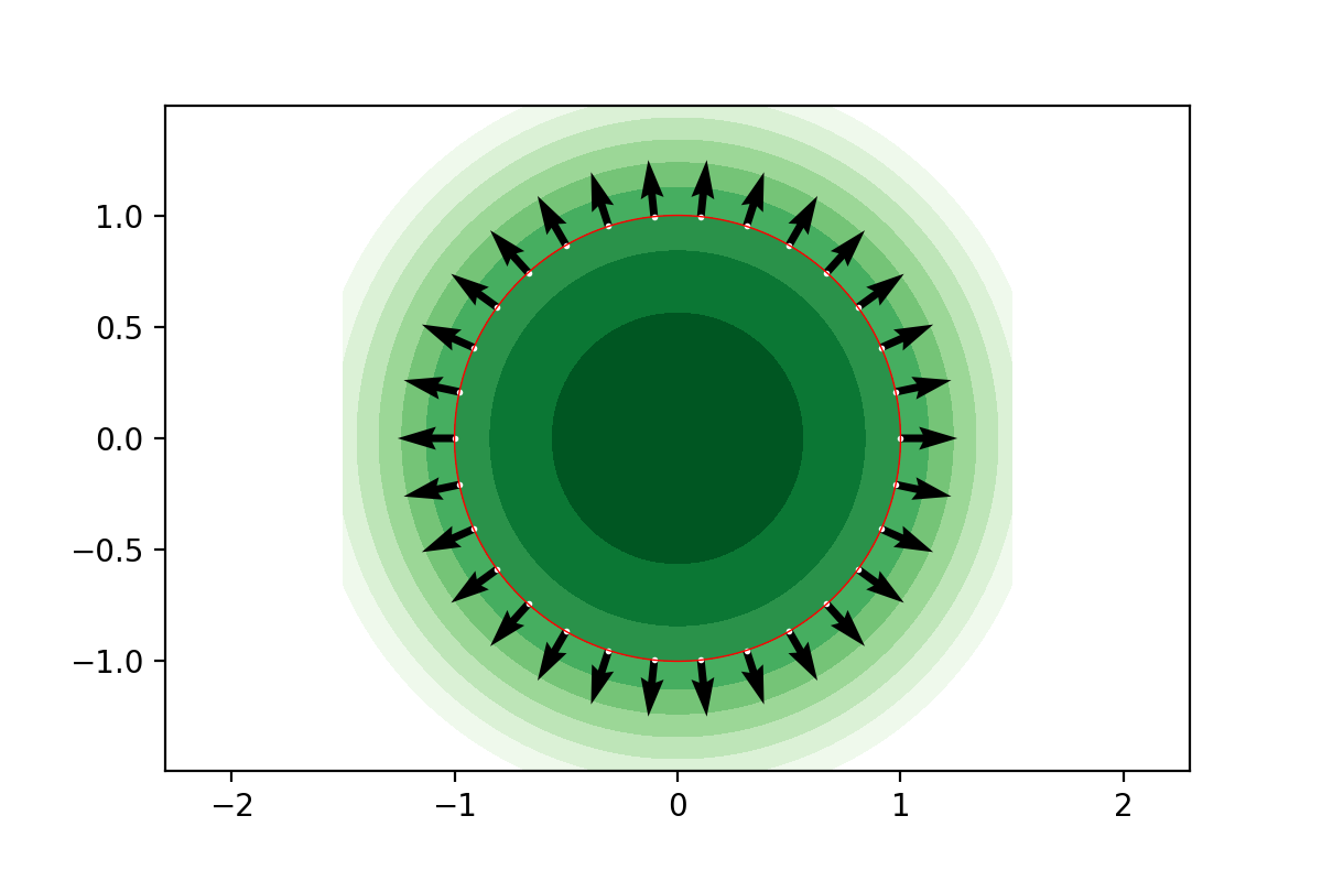
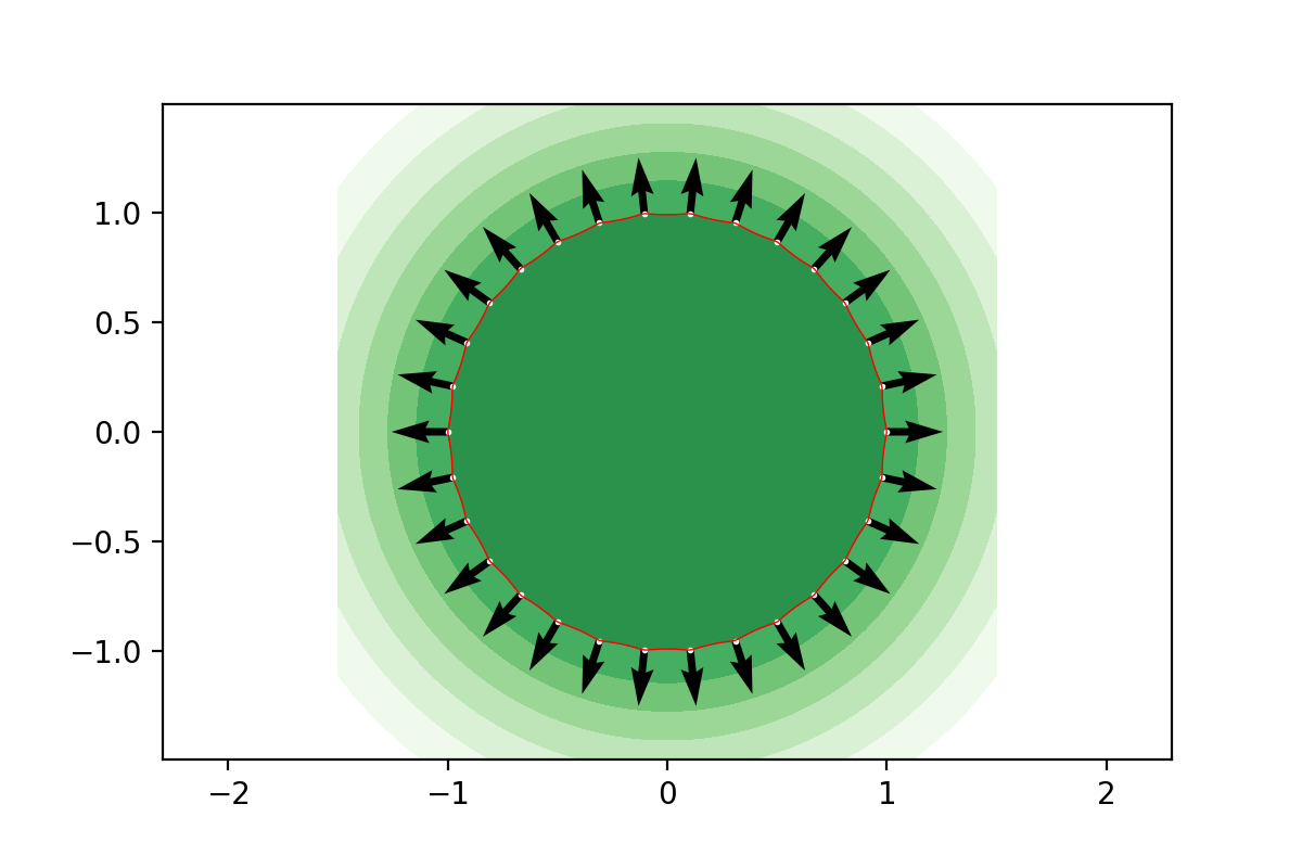
Figure 1. The top row depicts level lines of the signature function of the 30 white points and the implied normals obtained using the Gaussian kernel. The second row depicts the same for the Laplace kernel. The experiments in the first column correspond to no regularization ($\alpha=0$), where $\alpha=10^{-10}$ for the ones in the right column.

Next we consider a non-smooth curve, the boundary of a square. This example shows how the Laplace kernel can more closely follow the boundary as it generates a solution of a PDE that is merely continuous.

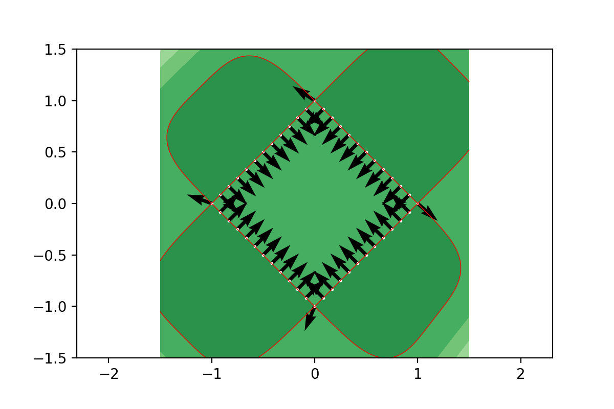
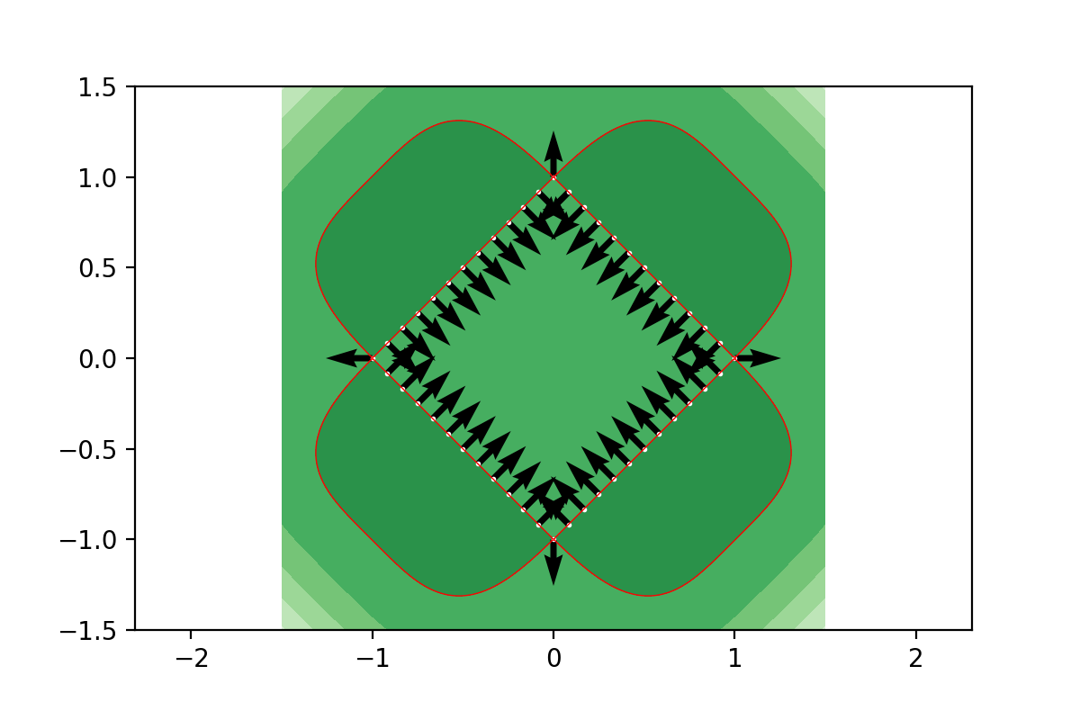
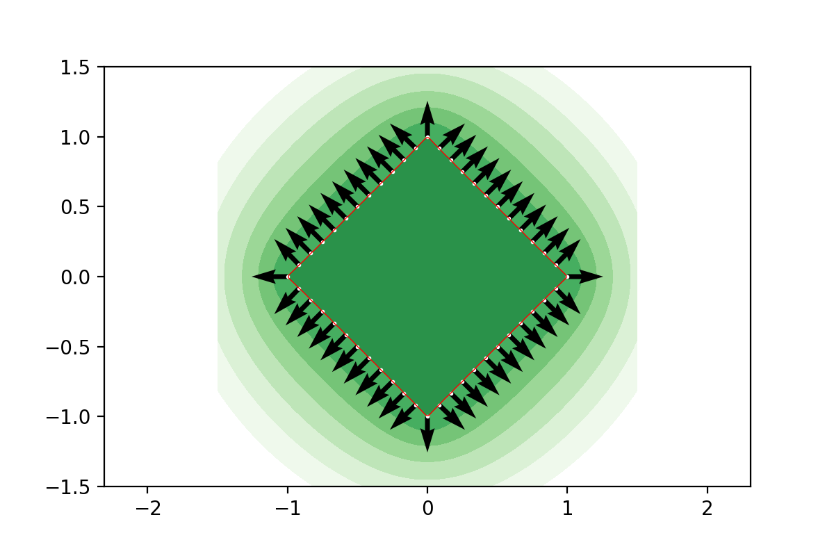
Figure 2. The top row depicts level lines of the signature function of the 48 white points and the implied normals obtained using the Gaussian kernel. The second row depicts the same for the Laplace kernel. The experiments in the first column correspond to no regularization ($\alpha=0$), whereas $\alpha=10^{-10}$ for the ones in the right column.

It is interesting to observe how the level lines of the signature function obtained with the Gauss kernel can also reproduce the square but since the signature function is analytic it does so by splitting the whole curve into two smooth closed curves, of which union the square is part of. We shall soon see that this does not prevent the use of the Gauss kernel in more general circumstances but leads to the need of using regularization to control the shape of level lines. Again it is apparent how the level lines smooth out and simplify away from the non-smooth curve considered. In Table 1 we compute the error between the exact and implied curvatures for a sector of a unit circle of angle $\frac{\pi}{16}$ for both the Gauss and Laplace kernels. It shows the high accuracy achieved with relatively few points by the Gauss kernel. It also showcases the ability of the (regularized) Laplace kernel to obtain a good approximation. We restrict the error analysis to the middle quarter of the sector since the accuracy deteriorates in the regions around the end points. It is also apparent that the accuracy of the unregularized Gauss kernel saturates (due to the increasing ill-conditioning of the discrete system), while regularization is essentially unnecessary for the Laplace kernel, again due to the fact that the discrete system corresponds to a differential operator of “minimal order” and leads to significantly less ill-conditioning.

Method/Points		32	64	128	256
Gauss	$\alpha=0$	$2.26\times 10^{-6}$	$2.16\times 10^{-6}$	$1.54\times 10^{-6}$	$5.51\times 10^{-6}$
	$\alpha=10^{-10}$	$5.47\times 10^{-4}$	$2.78\times 10^{-4}$	$1.24\times 10^{-4}$	$4.22\times 10^{-5}$
Laplace	$\alpha=0$	$4.84$	$0.24$	$5.12\times 10^{-4}$	$1.01\times 10^{-6}$
	$\alpha=10^{-10}$	$4.84$	$0.24$	$5.12\times 10^{-4}$	$7.55\times 10^{-7}$

Table 1. The average relative error between the exact and the implied curvature at the points found in the middle quarter of a sector of the unit circle of aperture $\frac{\pi}{16}$.

These experiments show the respective benefits of the two kernels. The Gauss kernel delivers an analytic signature which attempts to place the data points on a union of smooth curves, while the Laplace kernel leads to a merely continuous signature which can therefore exhibit level sets that more closely follow the data points, even as they go through corners (singularities in general). This will be even more evident in the experiments depicted in Figures 3-6 and 7-9, where the data points are randomly displaced from their original position along the circle and along the boundary of the square. The new points are obtained from the old ones by adding a displacement of 5%, 10%, and 50% which is uniform in direction and in distance. The percentage refers to maximal displacement size as a fraction of the maximal distance between consecutive data points. In this way, the error is directly related to the data set, which is in general all that is available. Notice, however, that the ordering (parametrization) of the points is not in any way required knowledge for the construction of the signature function. Figure 4 shows the realization of the random data sets with different level of noise for the experiments depicted in Figures 3-6 and 7-9 obtained by the use of the Gaussian kernel. The corresponding experiments with the Laplace kernel are based on a different realization of the perturbed data set that is not depicted in this paper.

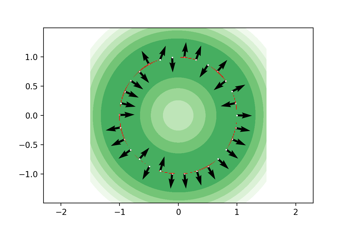
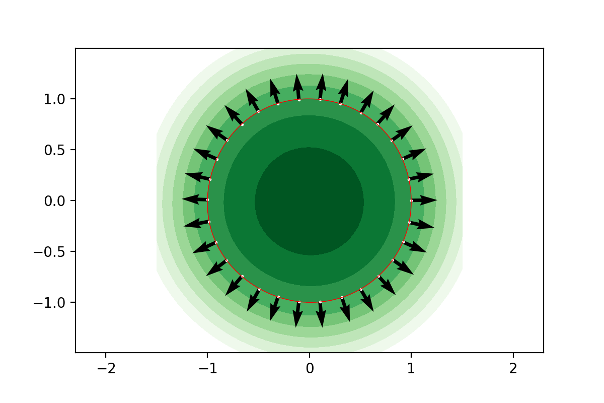
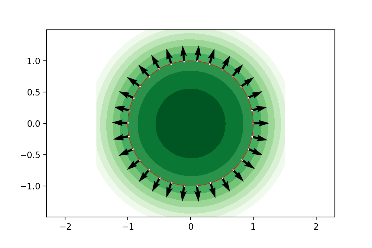
Figure 3. The circle example revisited by randomly displacing the original exact sample by 5% noise. Depicted are the level lines and implied normals obtained by means of the Gauss kernel based signature function compute with different regularization levels $\alpha=0,10^{-10},.01,.05,.1,.25$ in increasing order from top left to bottom right.

It is evident how the analytic signature tries to accomodate smooth level lines through the data without necessarily connecting the points in what the human eye would consider the natural way. Notice, however, how the implied normals can still approximately capture the tangent line to the “average curve”. The introduction of regularization, by allowing for approximate interpolation, makes it possible for the method to successfully connect the dots into a smooth line and capture its normal vector. In these and subsequent numerical experiments, the level line depicted in red is that corresponding the average value of the signature function on the data set.

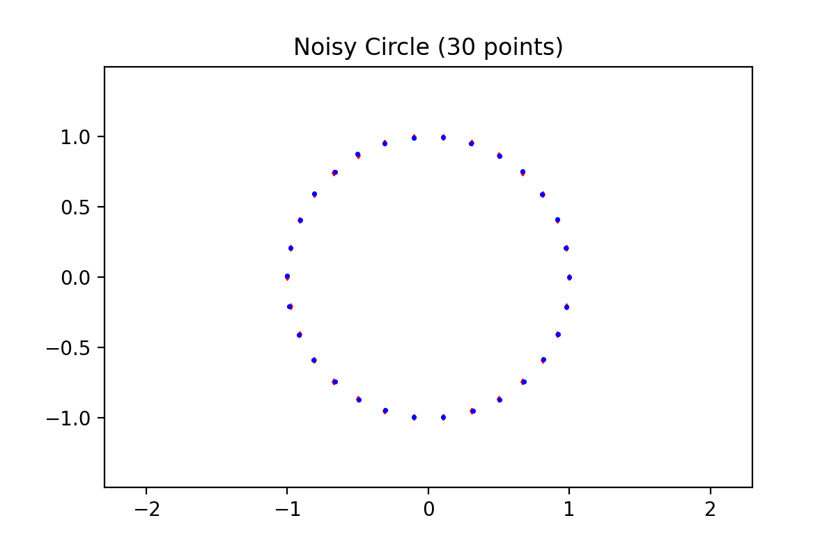
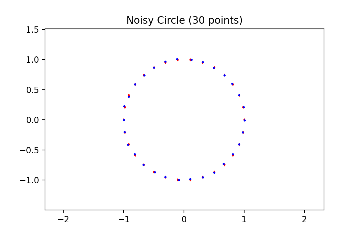
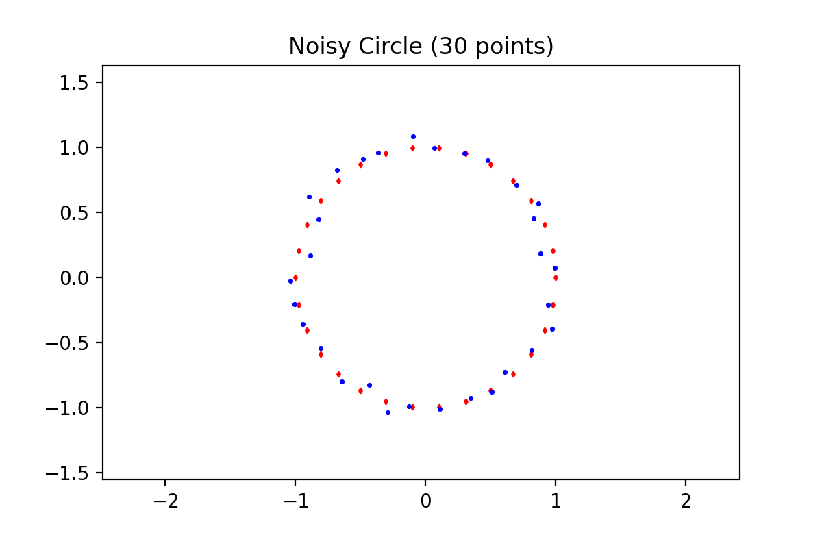
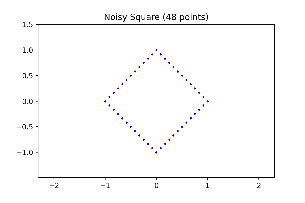
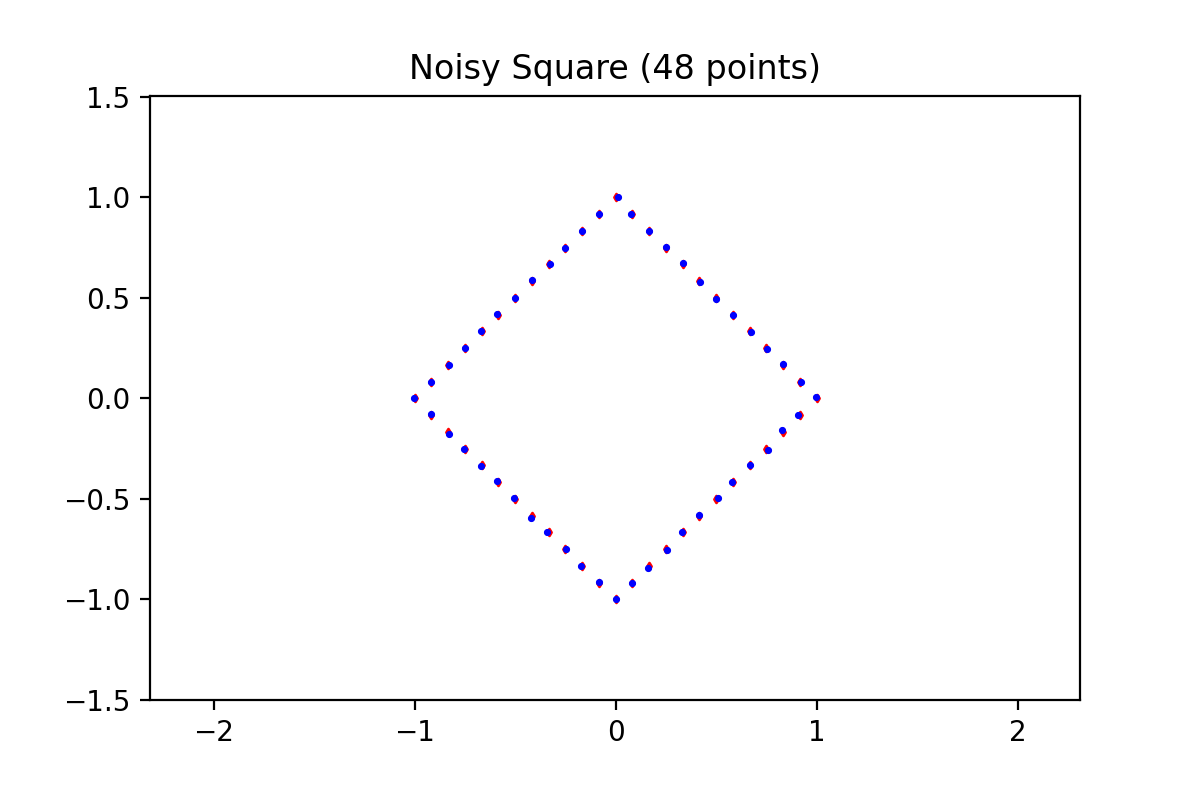
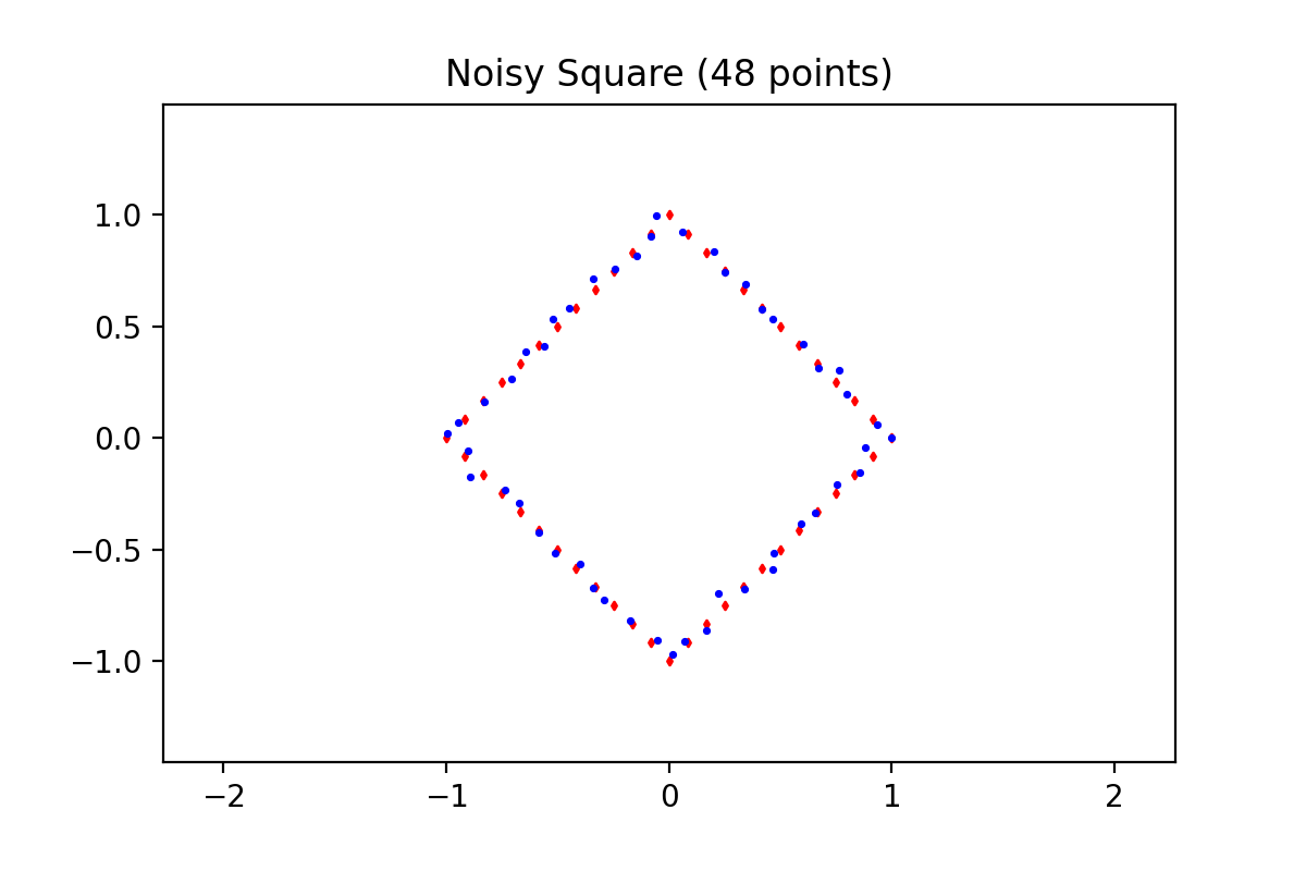
Figure 4. The original set of data points is shown in all images as red diamonds. The blue dots show the noise-perturbed data points at the different noise levels: 5%, 10%, and 50% from left to right.

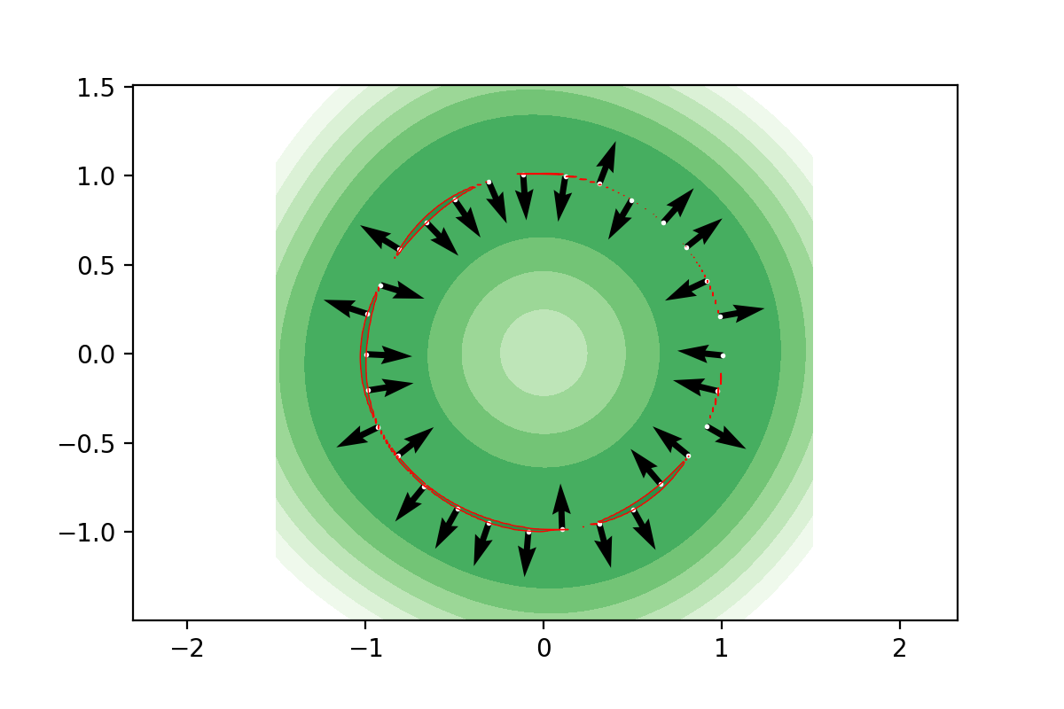
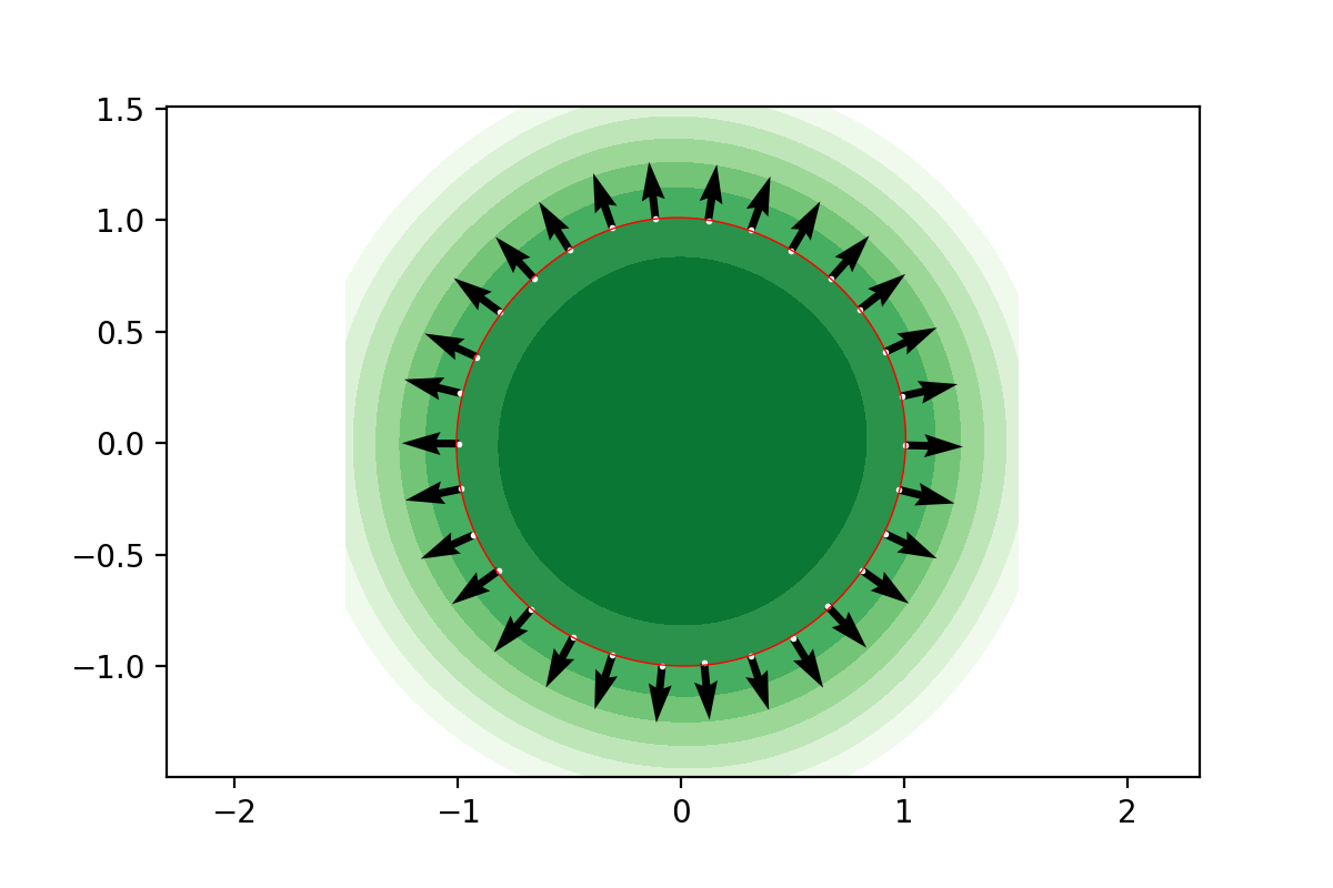
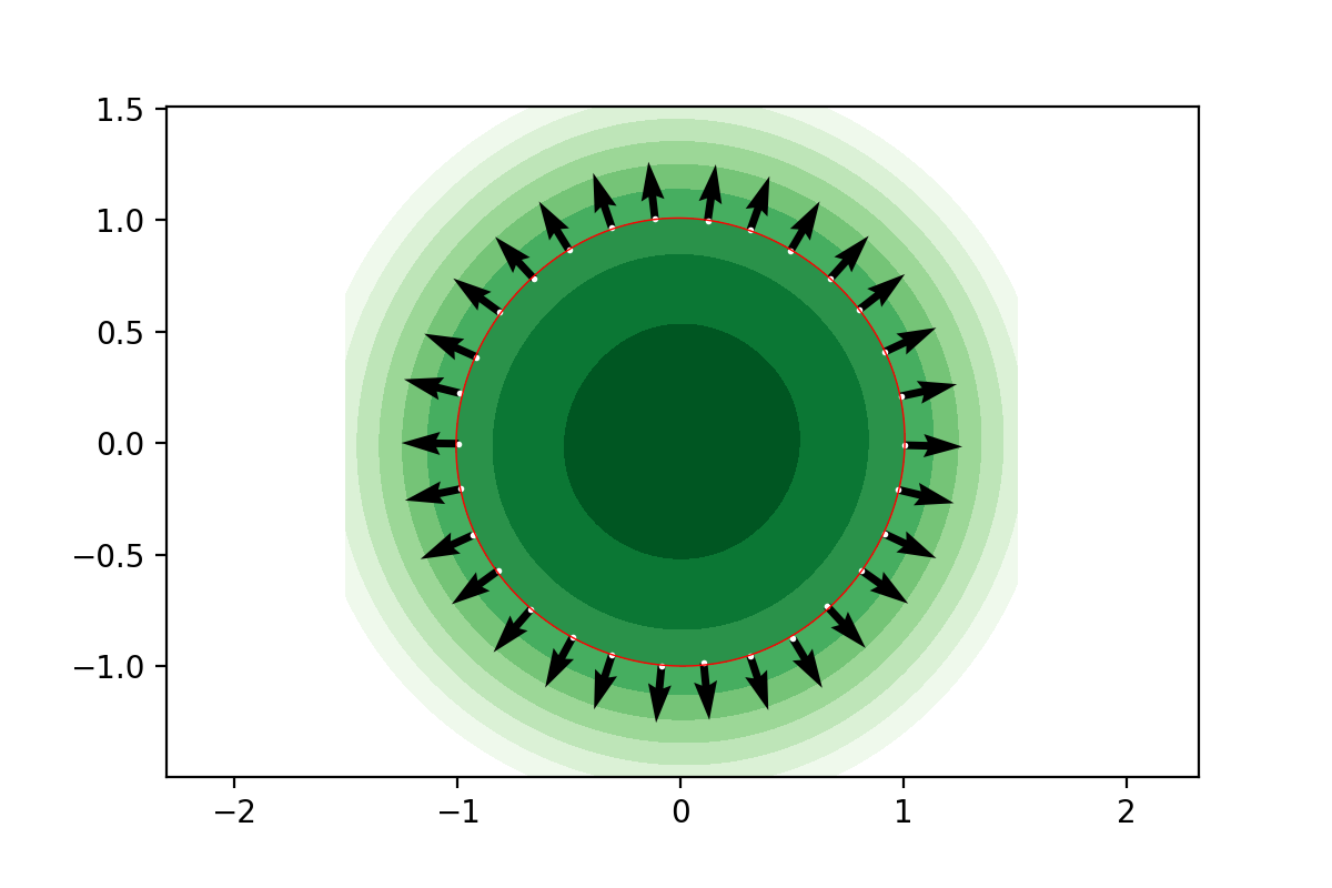
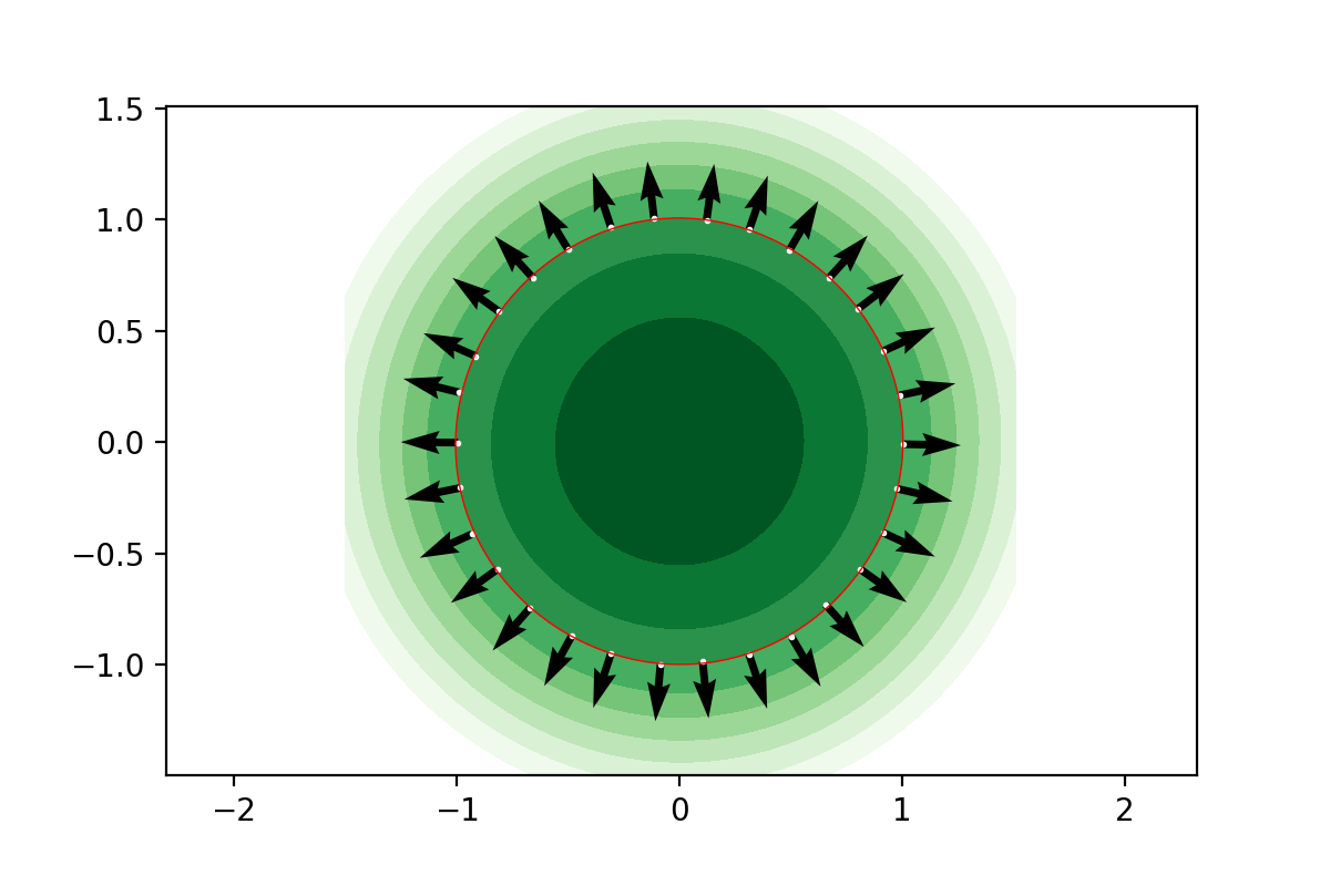
Figure 5. The circle example revisited by randomly displacing the original exact sample by 10% noise. Depicted are the level lines and implied normals obtained by means of the Gauss kernel based signature function compute with different regularization levels $\alpha=0,10^{-10},.01,.05,.1,.25$ in increasing order from top left to bottom right.

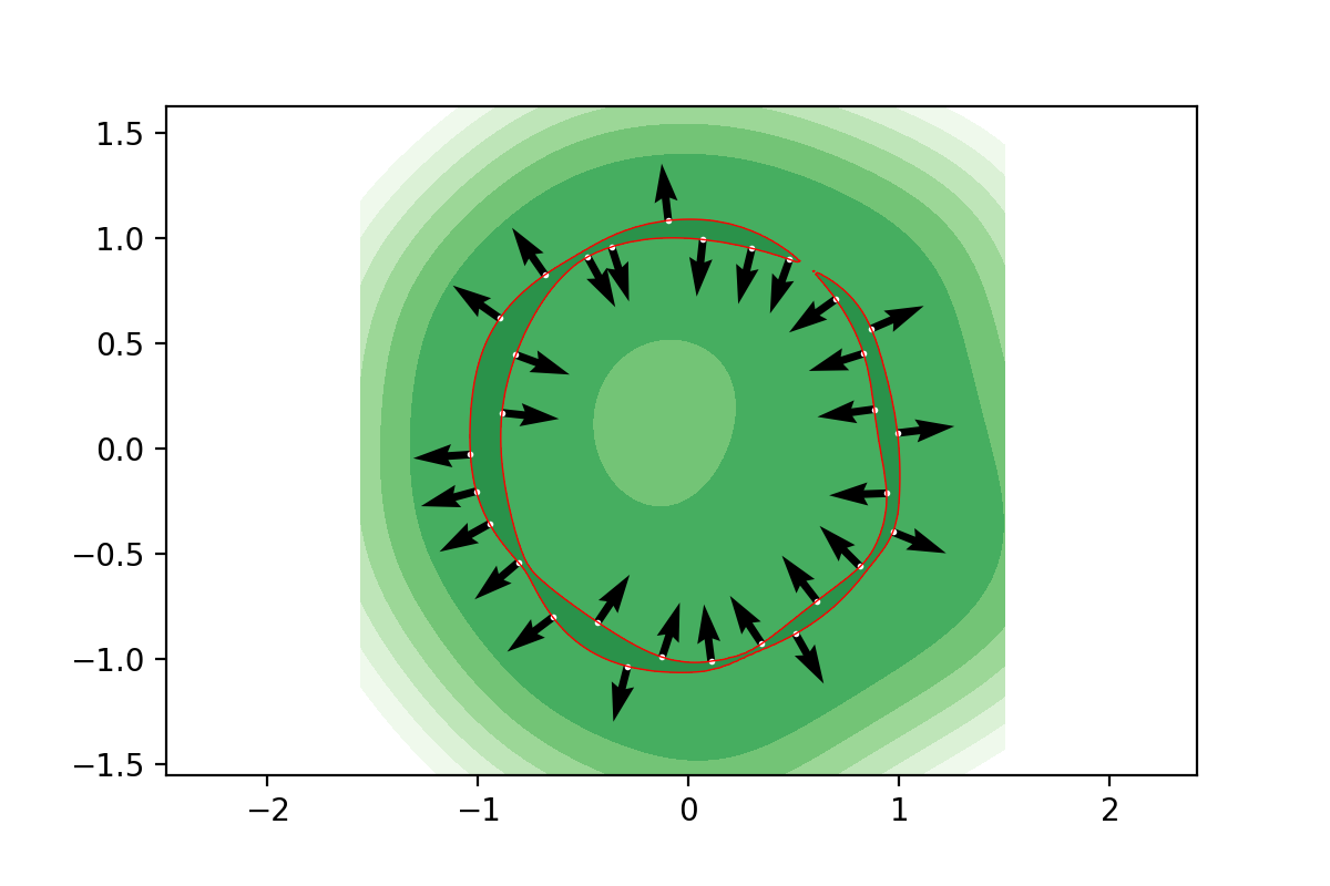
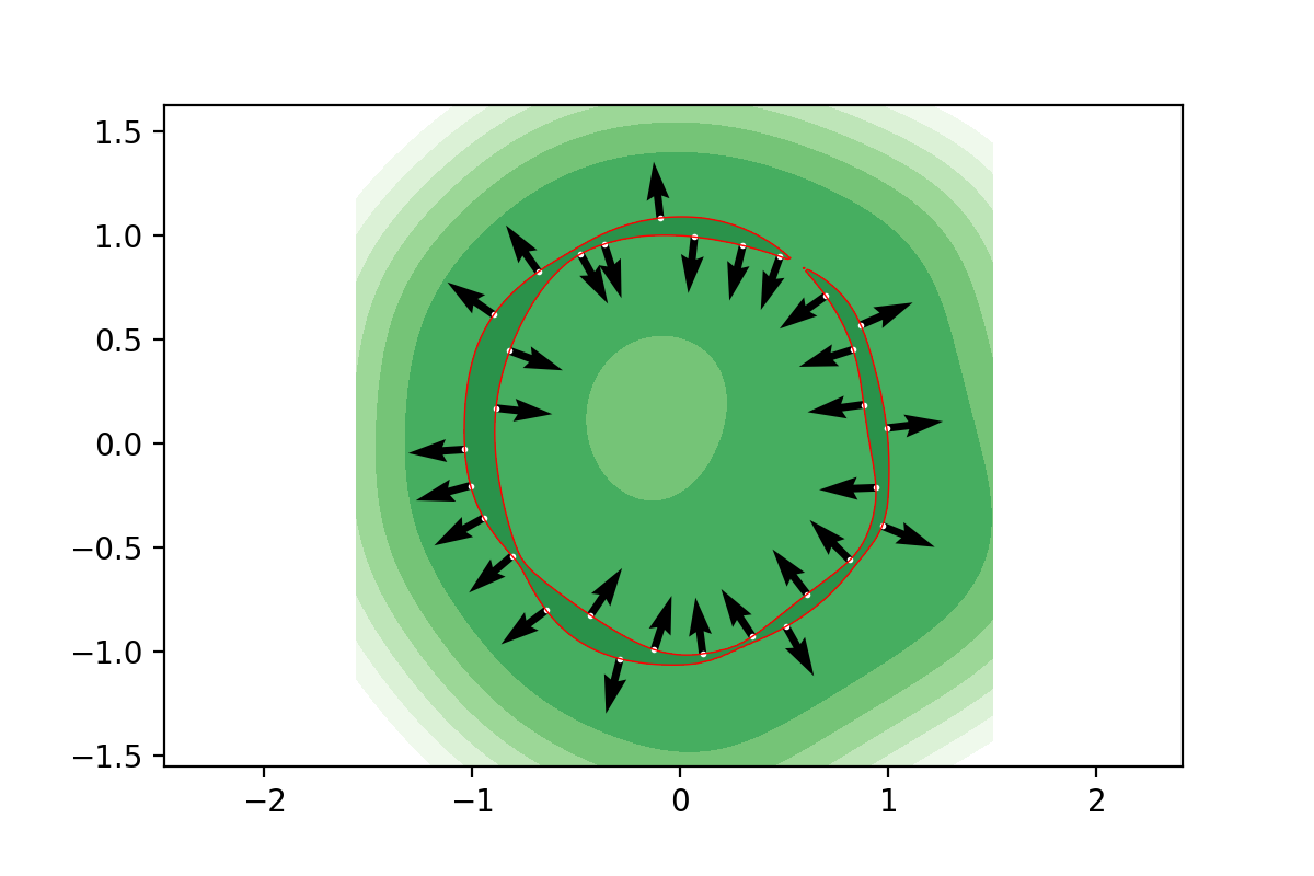
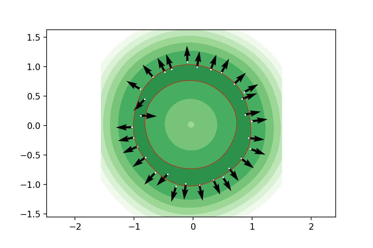
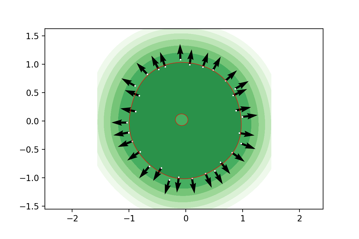
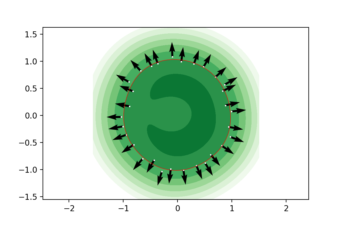
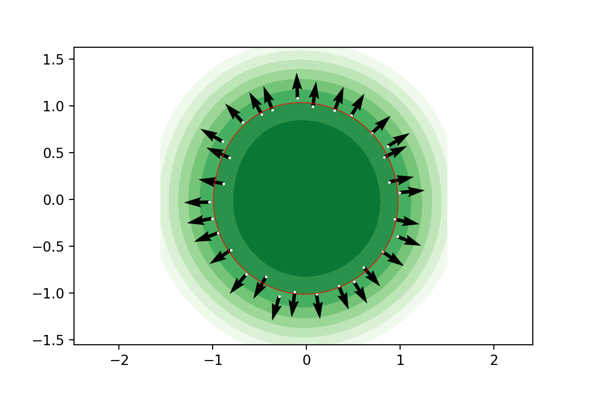
Figure 6. The circle example revisited by randomly displacing the original exact sample by 50% noise. Depicted are the level lines and implied normals obtained by means of the Gauss kernel based signature function compute with different regularization levels $\alpha=0,10^{-10},.01,.05,.1,.25$ in increasing order from top left to bottom right.

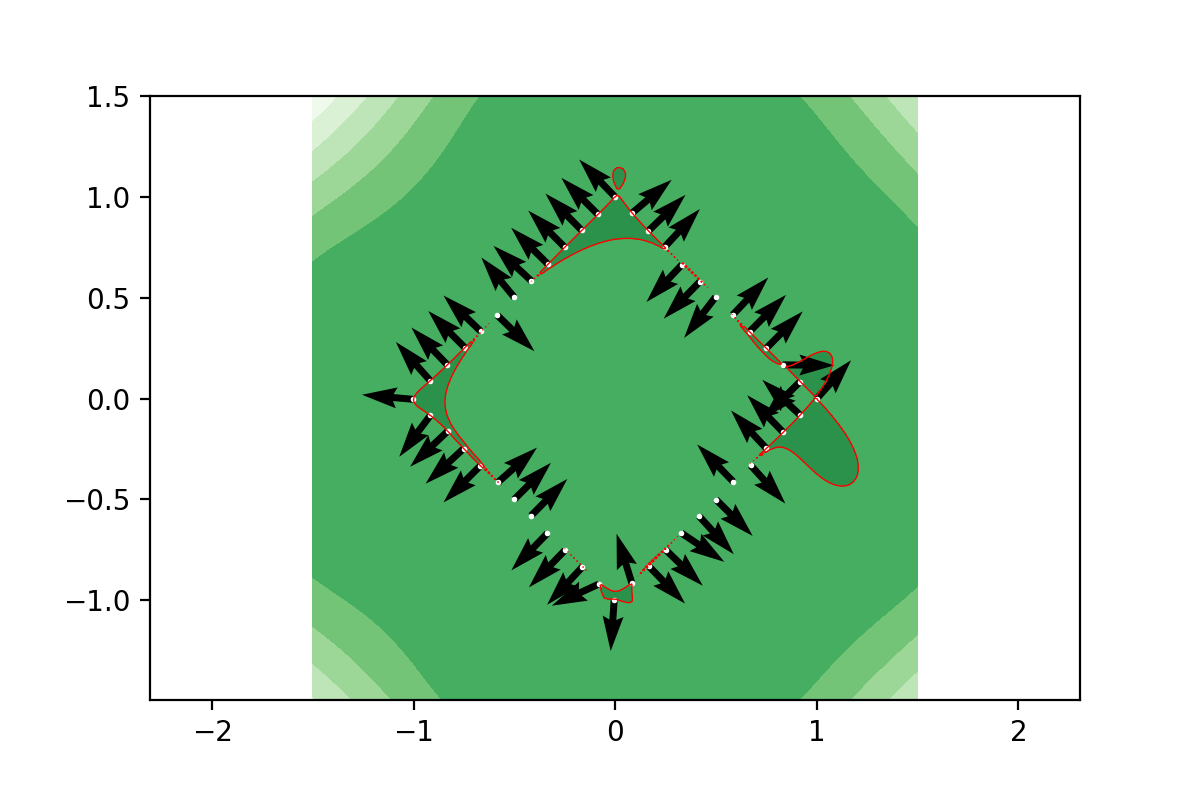
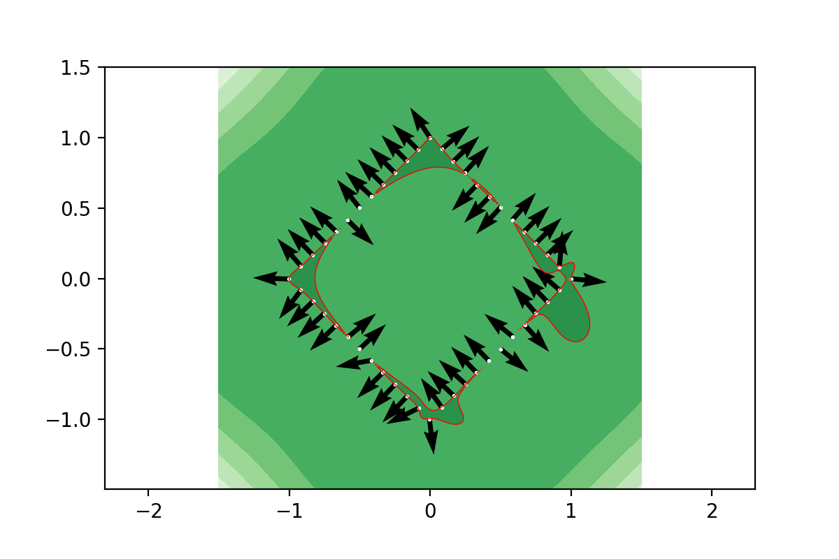
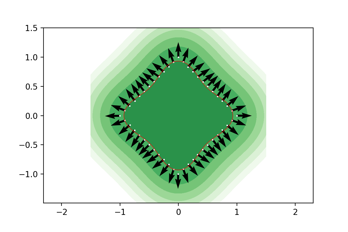
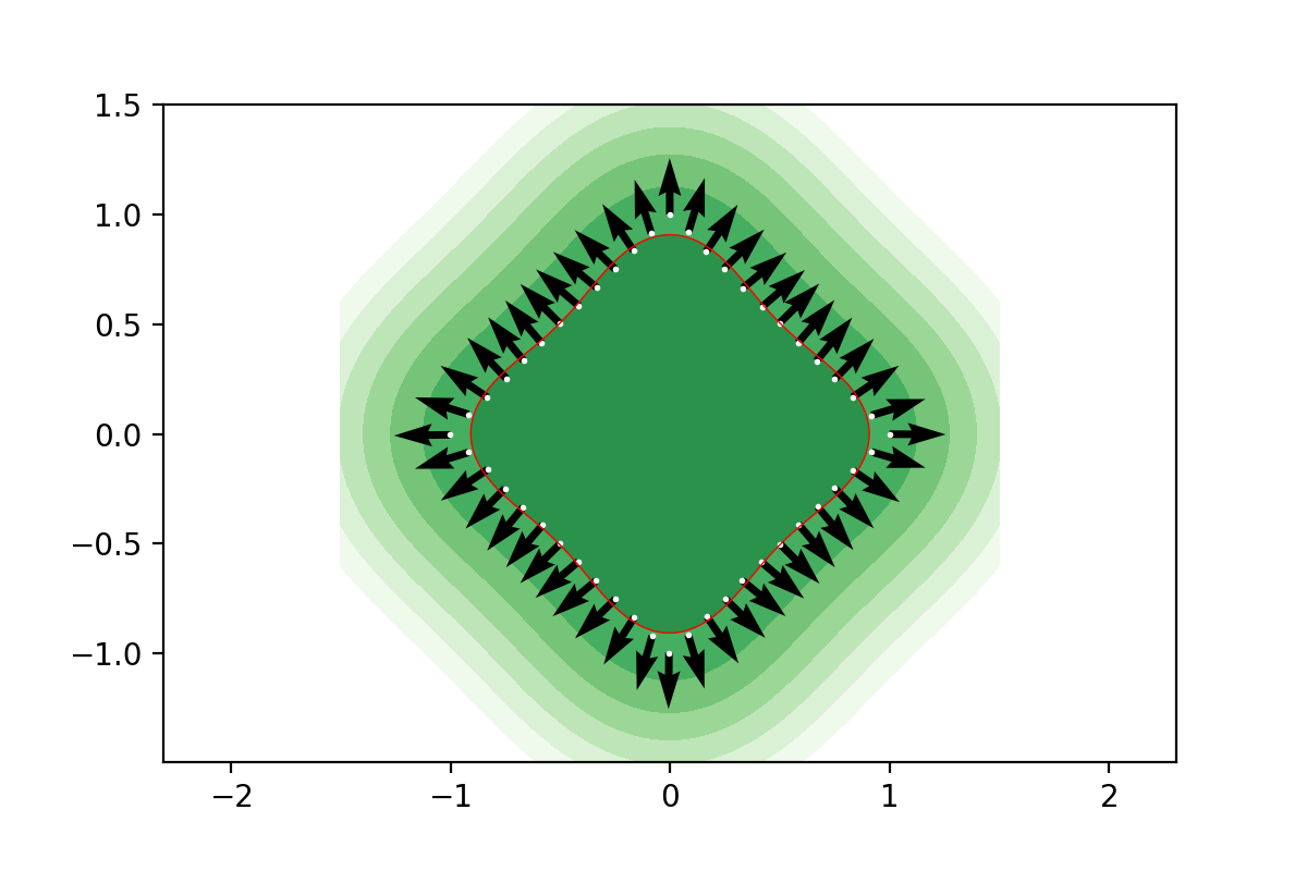
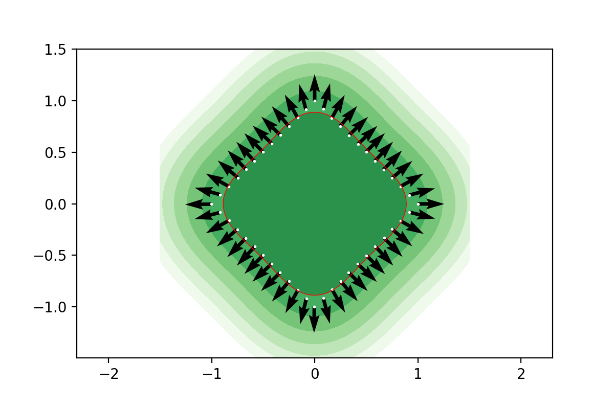
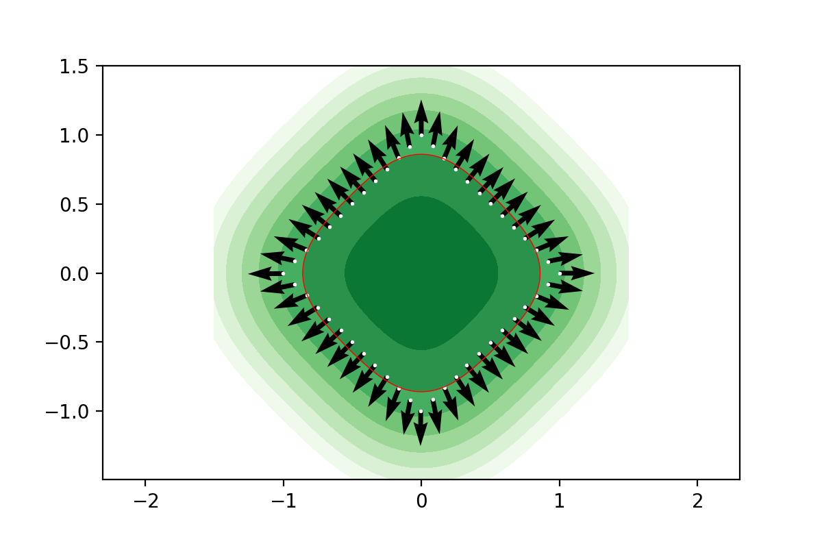
Figure 7. The square example revisited by randomly displacing the original exact sample by 5% noise. Depicted are the level lines and implied normals obtained by means of the Gauss kernel based signature function compute with different regularization levels $\alpha=0,10^{-10},.01,.05,.1,.25$ in increasing order from top left to bottom right.

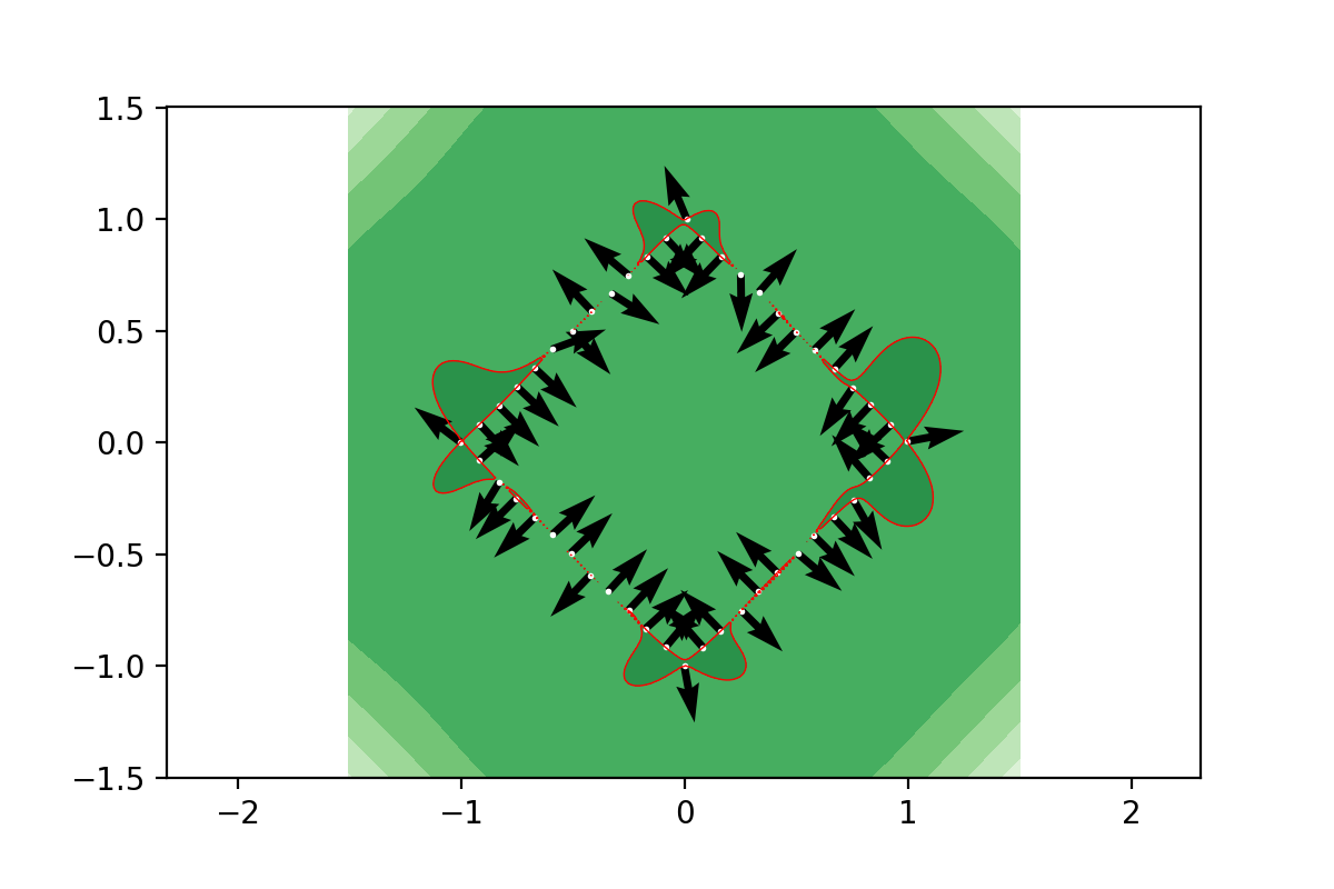
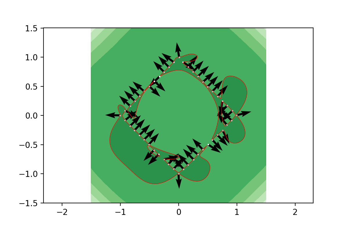
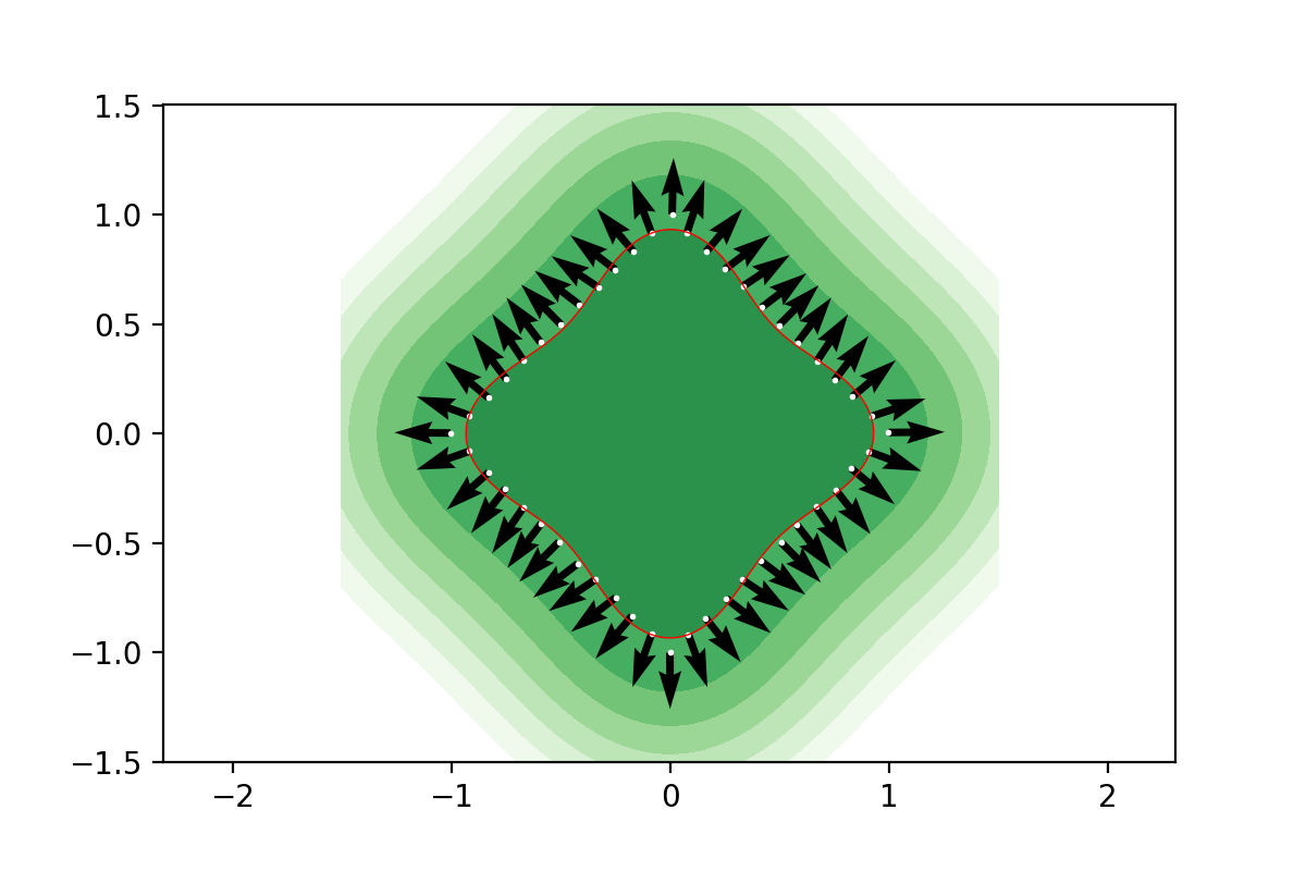
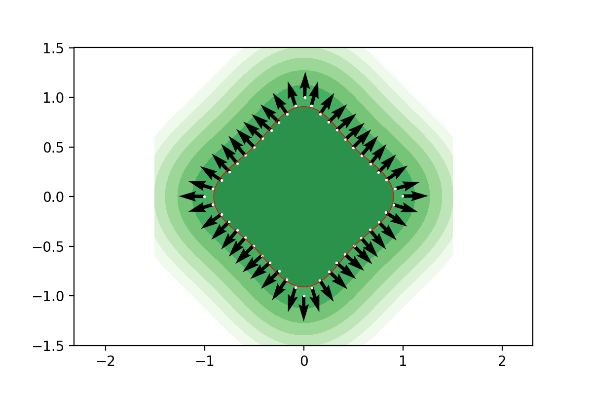
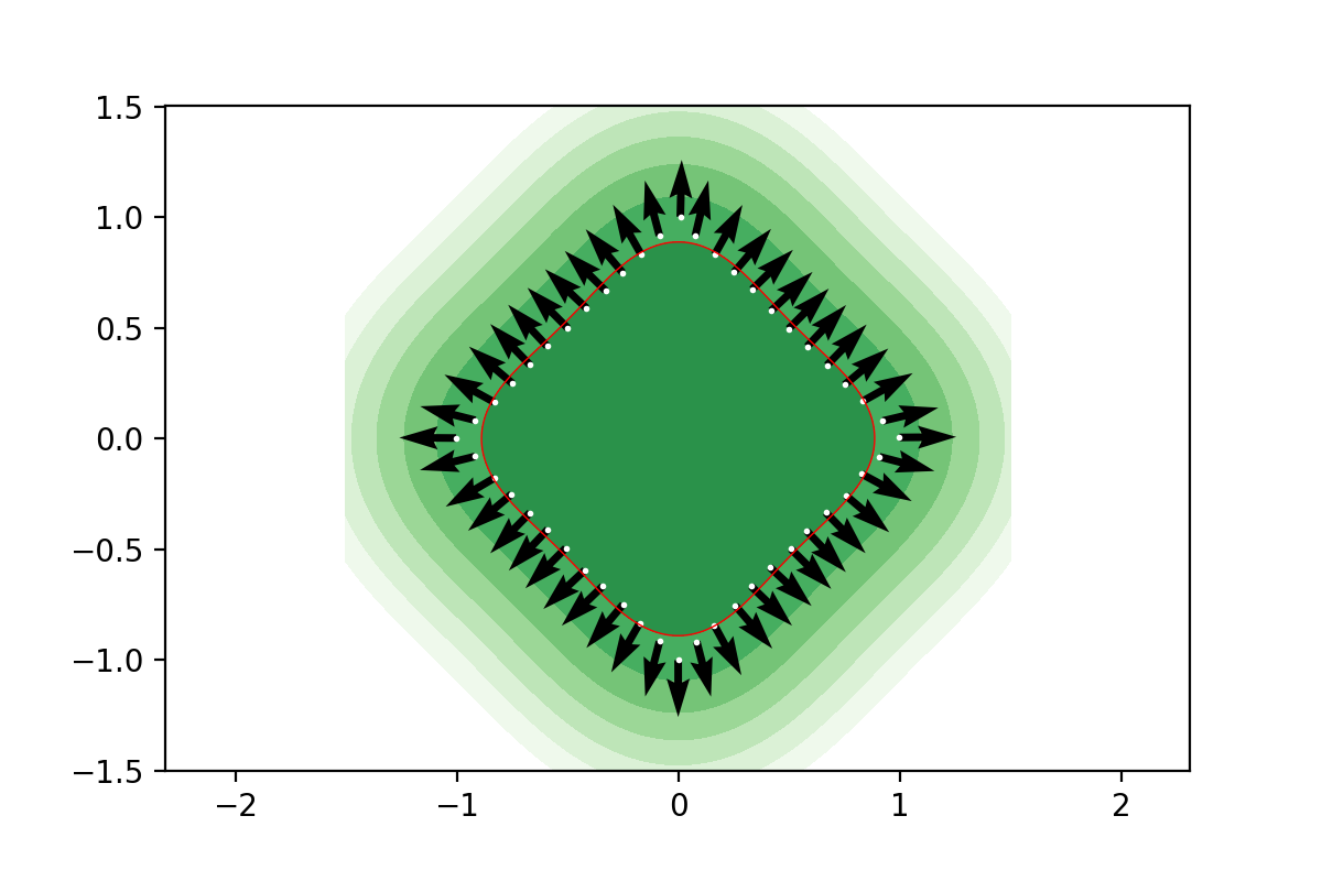
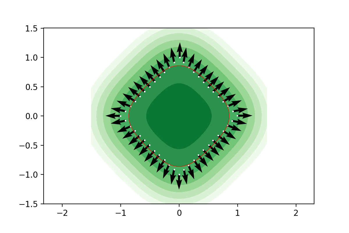
Figure 8. The square example revisited by randomly displacing the original exact sample by 10% noise. Depicted are the level lines and implied normals obtained by means of the Gauss kernel based signature function compute with different regularization levels $\alpha=0,10^{-10},.01,.05,.1,.25$ in increasing order from top left to bottom right.

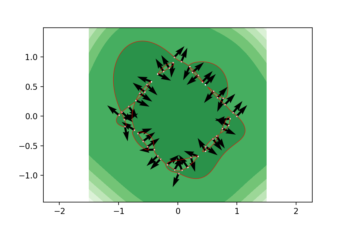
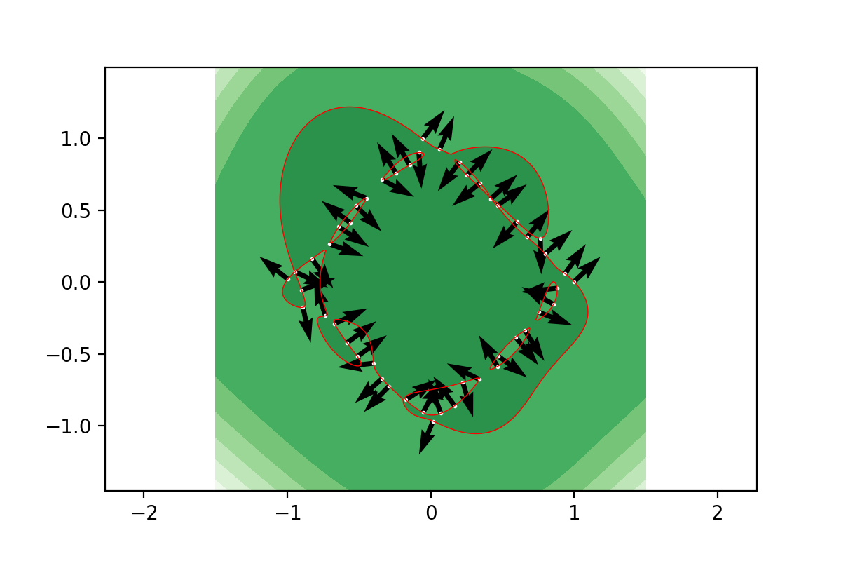
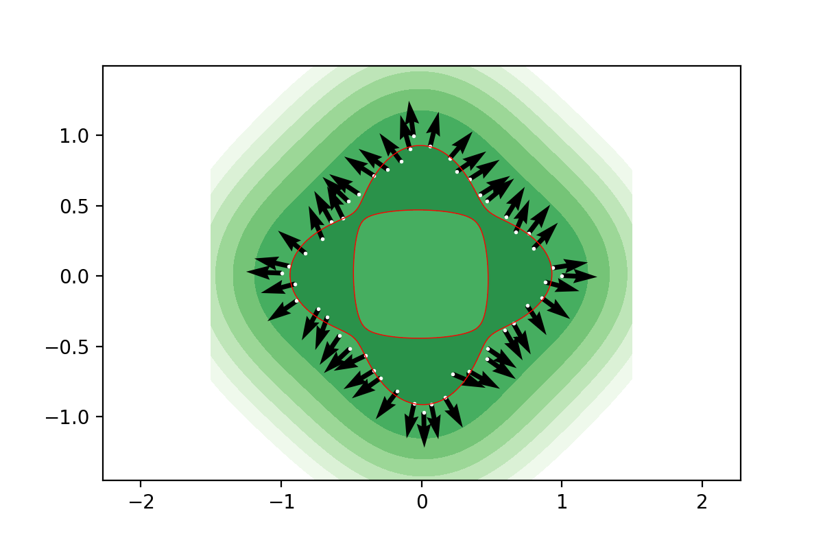
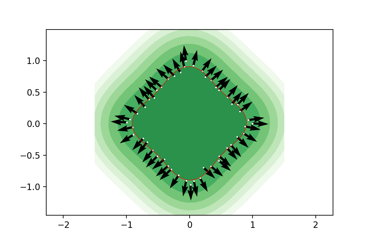
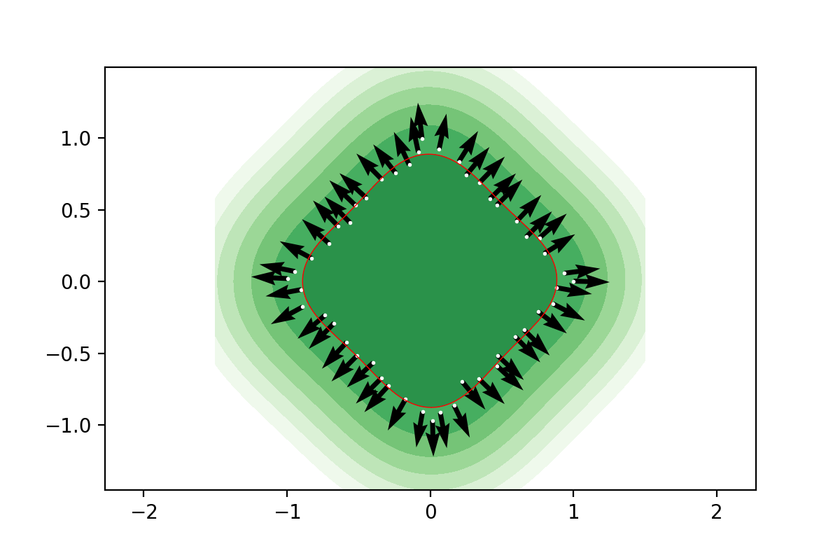
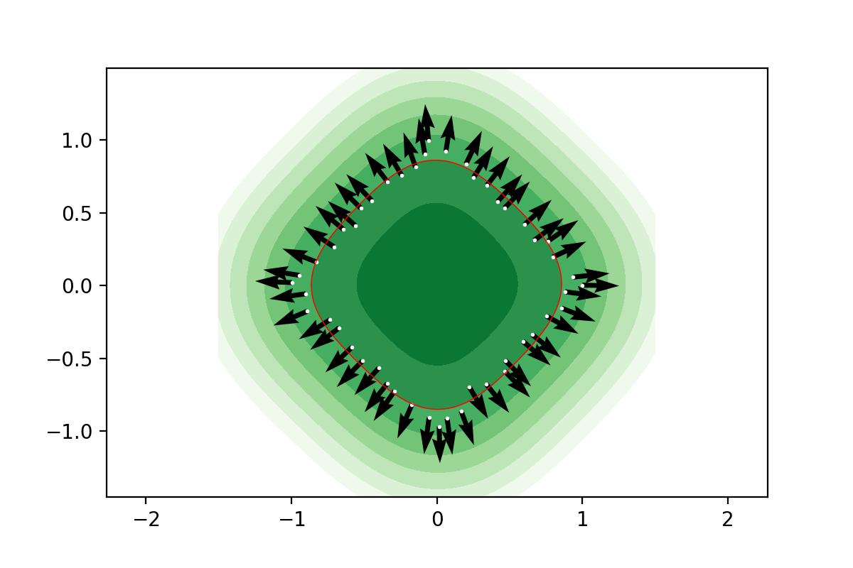
Figure 9. The square example revisited by randomly displacing the original exact sample by 50% noise. Depicted are the level lines and implied normals obtained by means of the Gauss kernel based signature function compute with different regularization levels $\alpha=0,10^{-10},.01,.05,.1,.25$ in increasing order from top left to bottom right.

Next we show in Figures 10-11 and Figures 12-13 the results of the same experiments that are obtained with the signature function built on the Laplace kernel but only with 10% and 50% noise levels. It is remarkable how the normals appear very stable across all choices of regularization. While the method does not need to acquire any specific knowledge of local neighborhoods of the data set, it can prove convenient to apply it locally when one is confronted with a very large (data) set. This especially true when some regularization is necessary and when using the Gaussian kernel which can lead to an overly simplified implied level set that interpolates all the data points. The experiments found in Figures 14 and 15 show the method applied to a non-smooth graph locally around the origin without and with noise. In Tables 2-3 we record the implied normals and curvatures computed at the origin with the Gauss kernel at various regularization and noise levels. Again the normal appears to be computed in a very stable manner across noise and regularization levels.

Noise/Regularization	0	$10^{-10}$	.01	.05	.1
0%	$(-.000002,1.)$	$(0.,-1.)$
5%	$(0.0568,-0.998)$	$(0.0025,-1.)$	$(-.000419,-1.)$	$(-.000368,-1.)$	$(-.000407,-1.)$
10%	$(.000892,1.)$	$(-0.0152,-0.9999)$	$(.000821,-1.)$	$(.000332,-1.)$	$(.000835,-1.)$
50%	$(0.016,1.)$	$(0.0885,0.996)$	$(0.0031-1.)$	$(-.000419,-1.)$	$(-0.00364,-1.)$

Table 2. Implied normal at the origin for the graph experiment.

Noise/Regularization	0	$10^{-10}$	.01	.05	.1
0%	$-4.$	$3.999$
5%	$40.10$	$3.0307$	$3.301$	$4.410$	$5.6205$
10%	$-4935$	$3.295$	$3.3$	$4.412$	$5.6385$
50%	$-0.9671$	$-10.52$	$3.359$	$4.513$	$5.764$

Table 3. Implied curvature at the origin for the graph experiment.

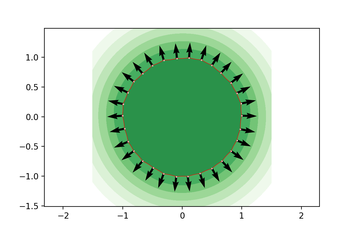
Figure 10. The circle example revisited by randomly displacing the original exact sample by 10% noise. Depicted are the level lines and implied normals obtained by means of the Laplace kernel based signature function compute with different regularization levels $\alpha=0,10^{-10},.01,.05,.1,.25$ in increasing order from top left to bottom right.

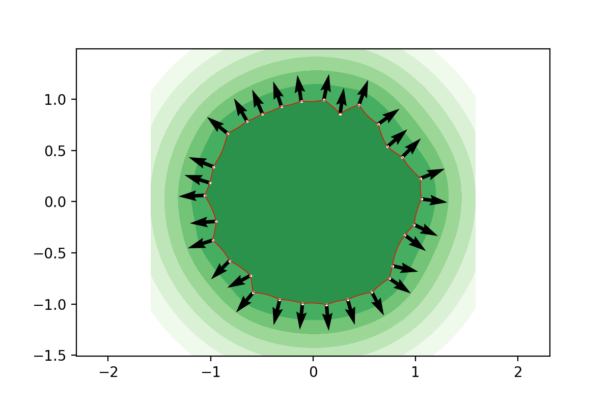
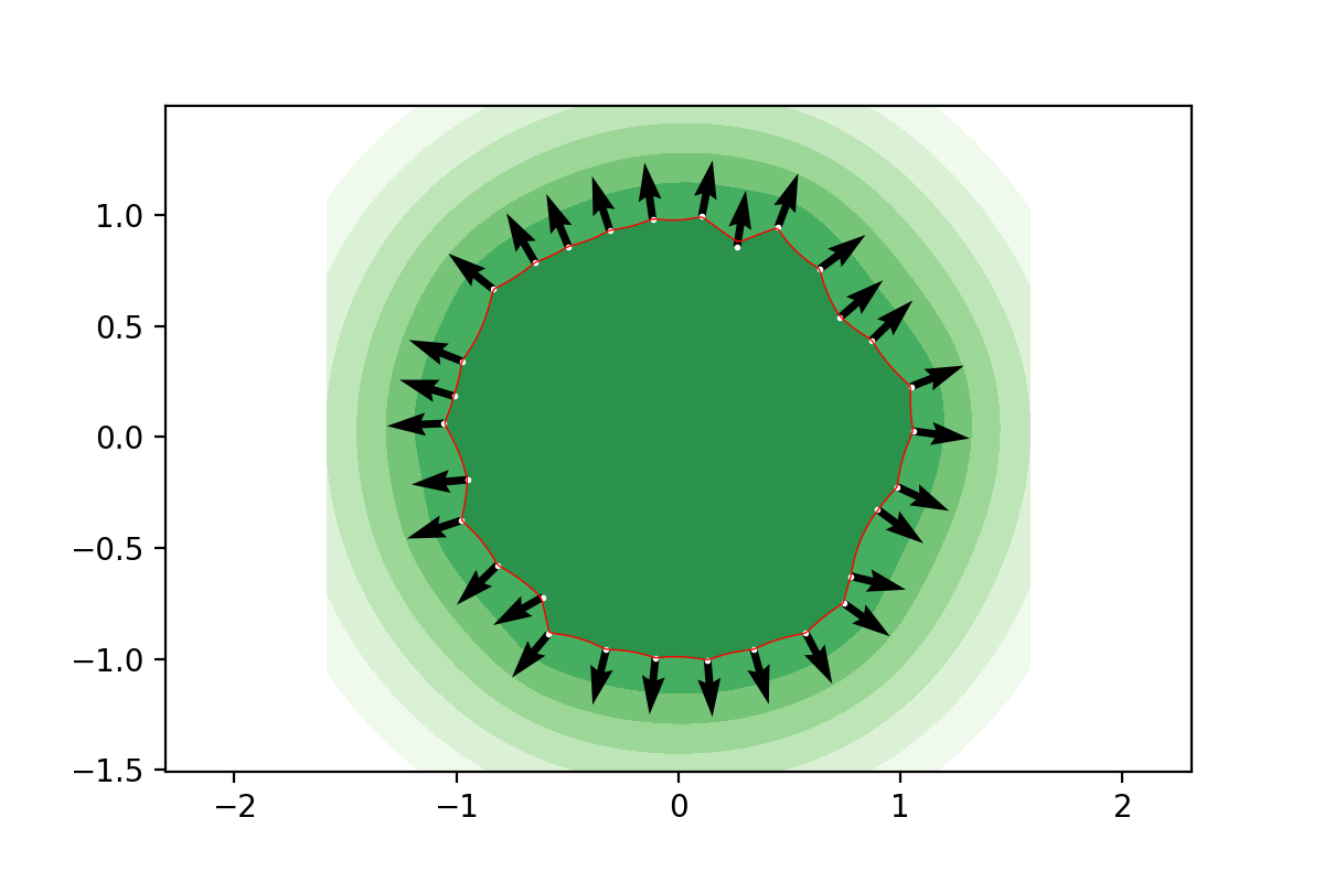
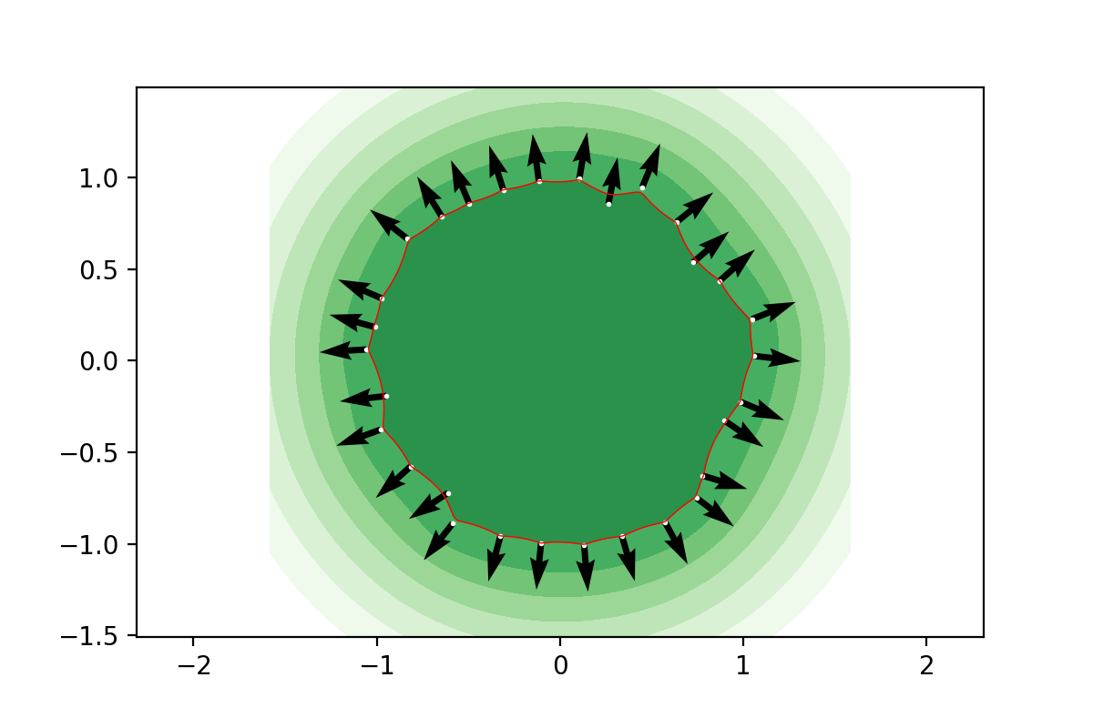
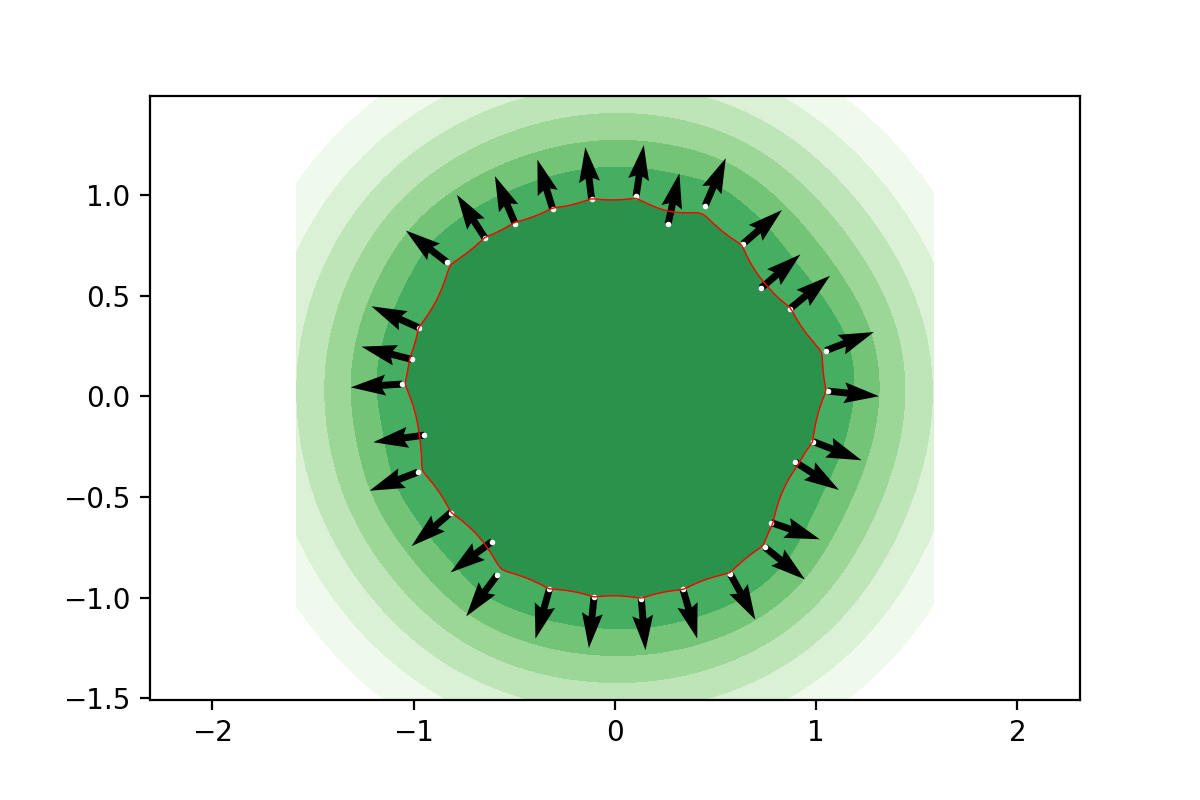
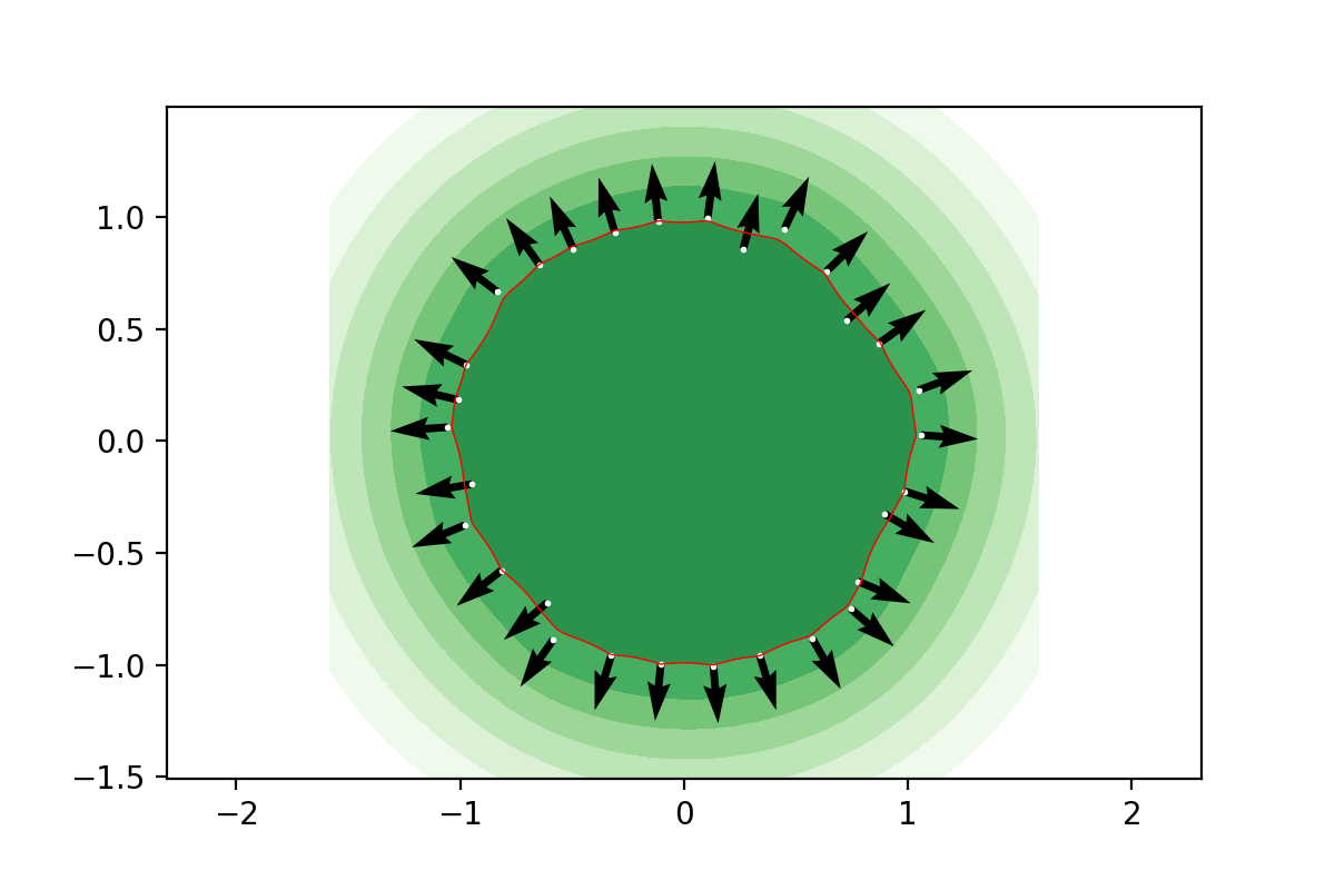
Figure 11. The circle example revisited by randomly displacing the original exact sample by 50% noise. Depicted are the level lines and implied normals obtained by means of the Laplace kernel based signature function compute with different regularization levels $\alpha=0,10^{-10},.01,.05,.1,.25$ in increasing order from top left to bottom right.

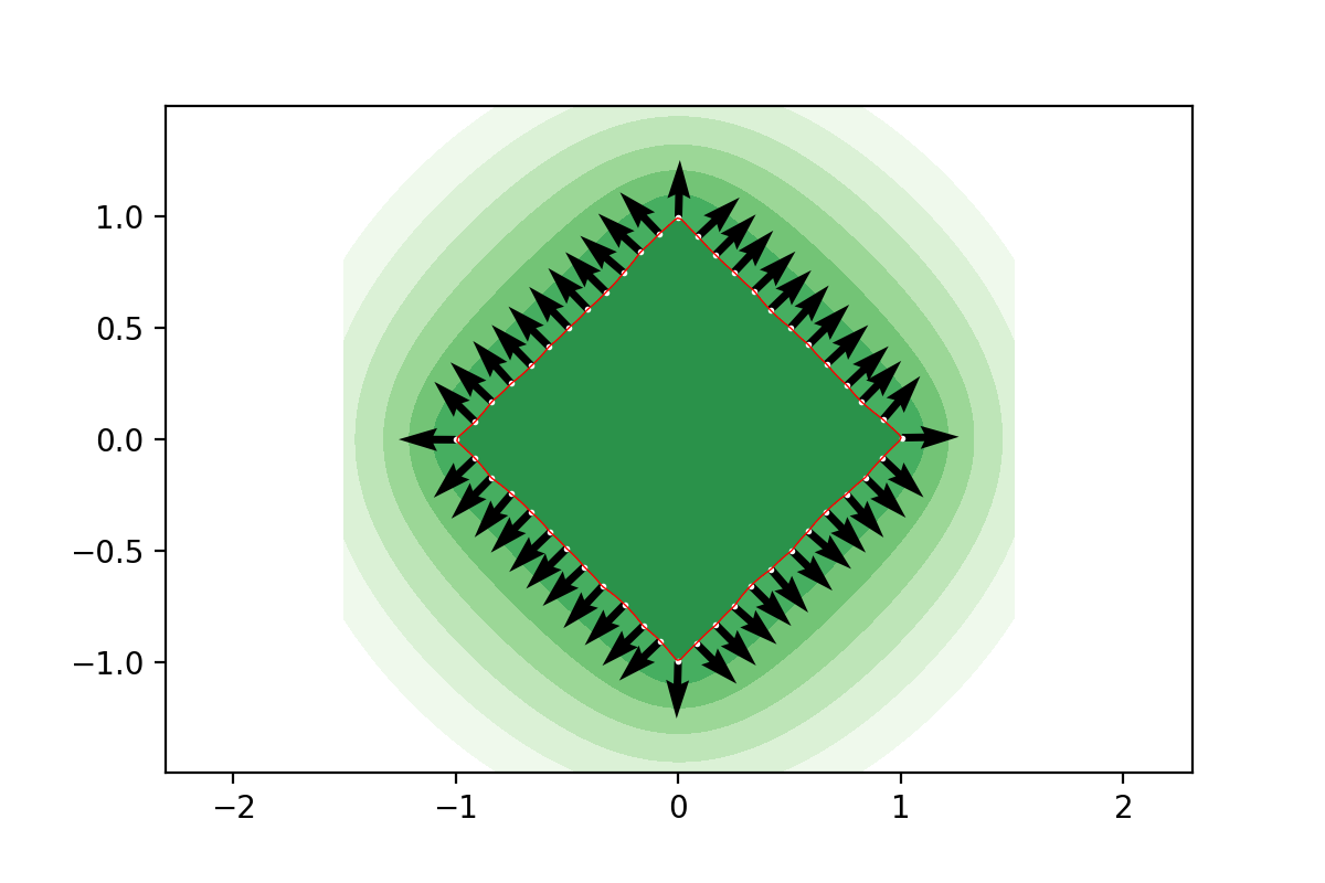
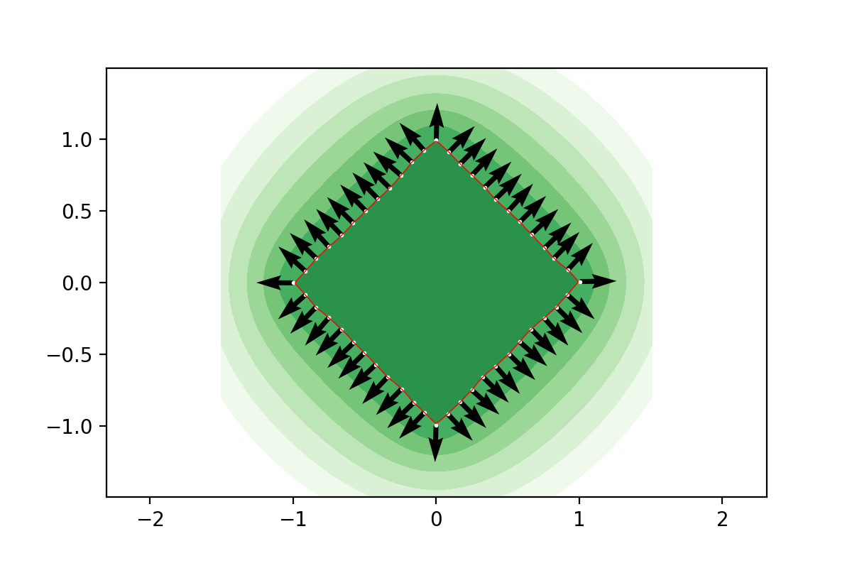
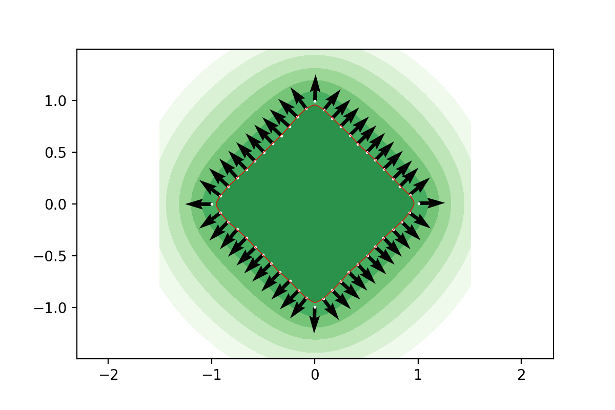
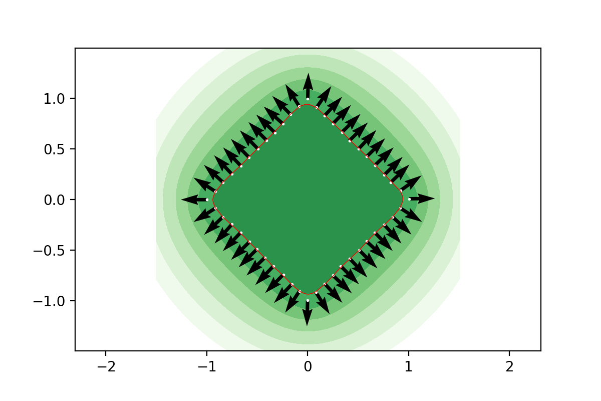
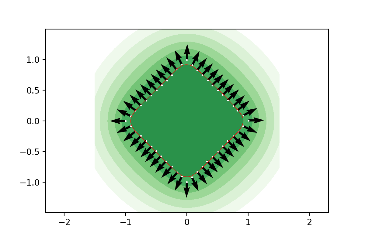
Figure 12. The square example revisited by randomly displacing the original exact sample by 10% noise. Depicted are the level lines and implied normals obtained by means of the Laplace kernel based signature function compute with different regularization levels $\alpha=0,10^{-10},.01,.05,.1,.25$ in increasing order from top left to bottom right.

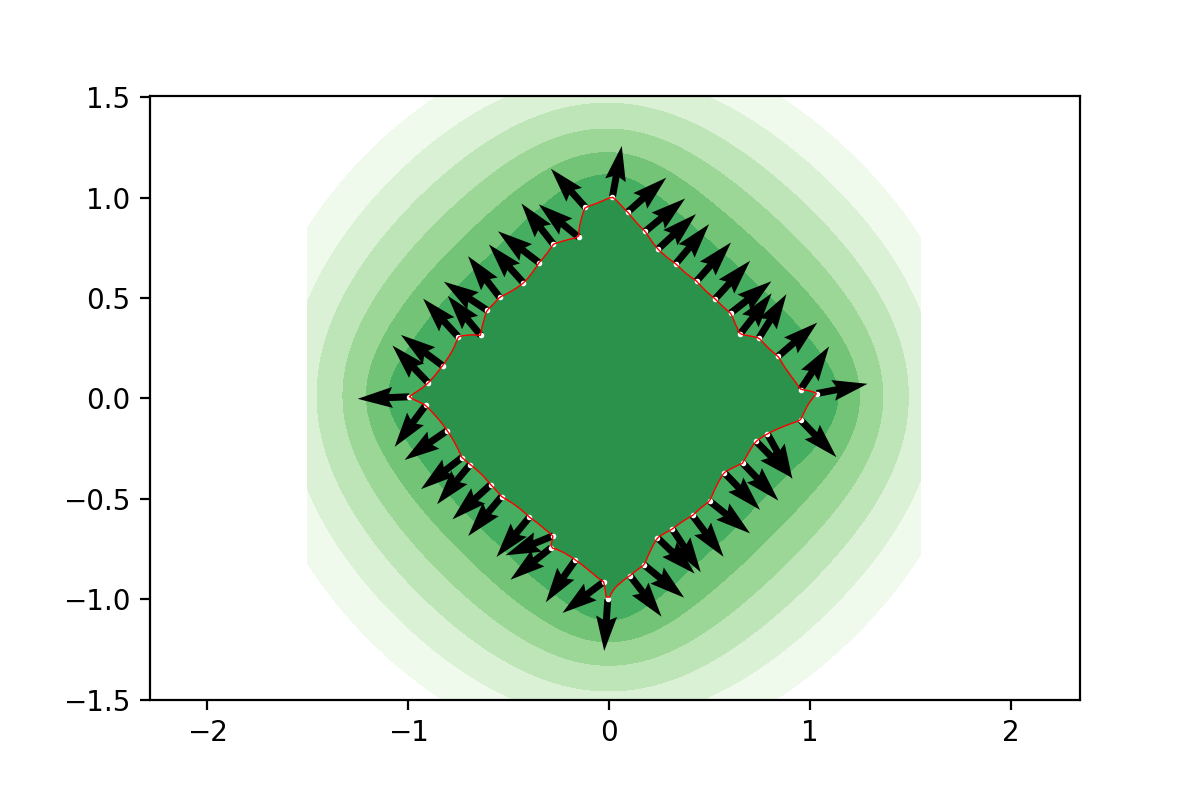
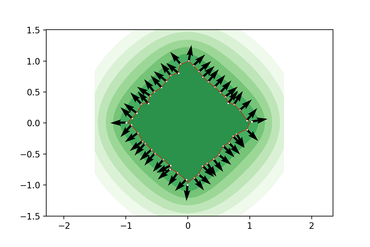
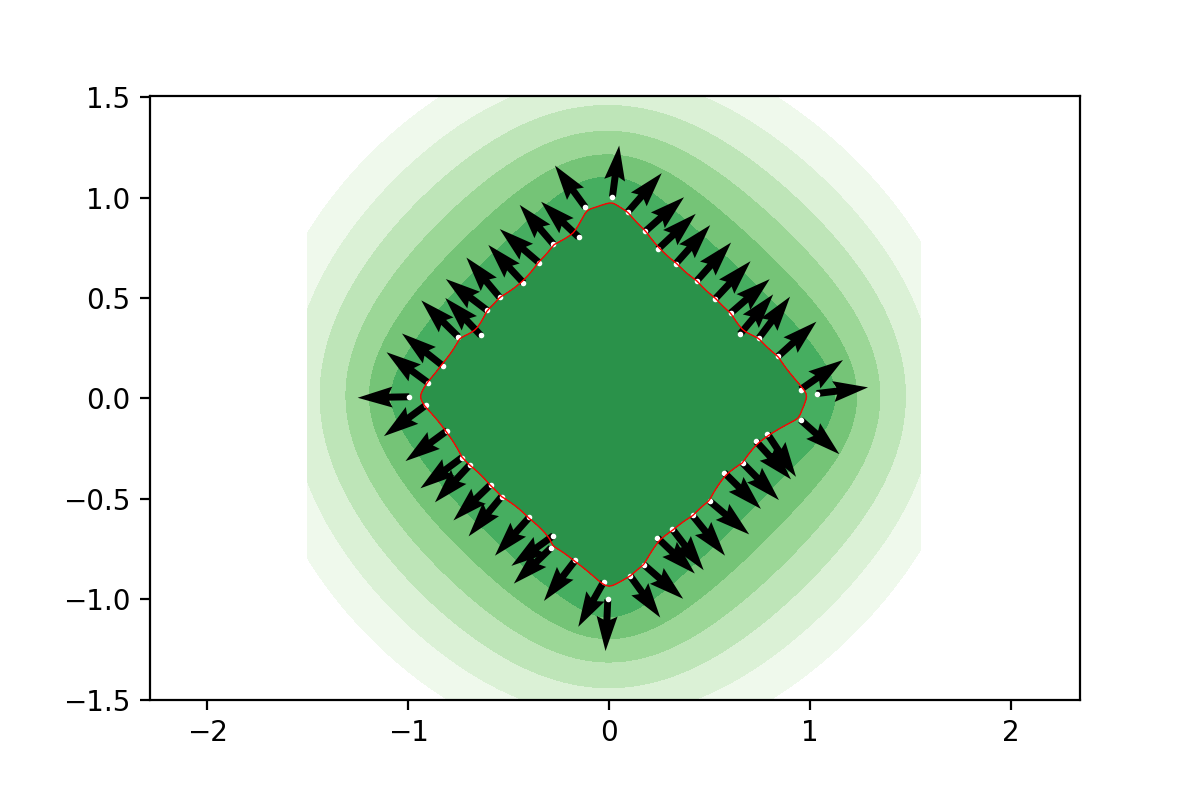
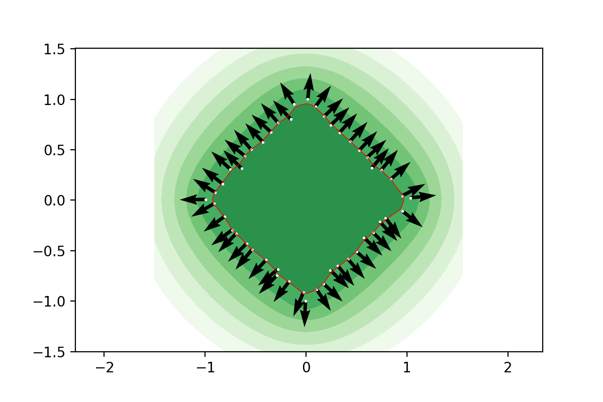
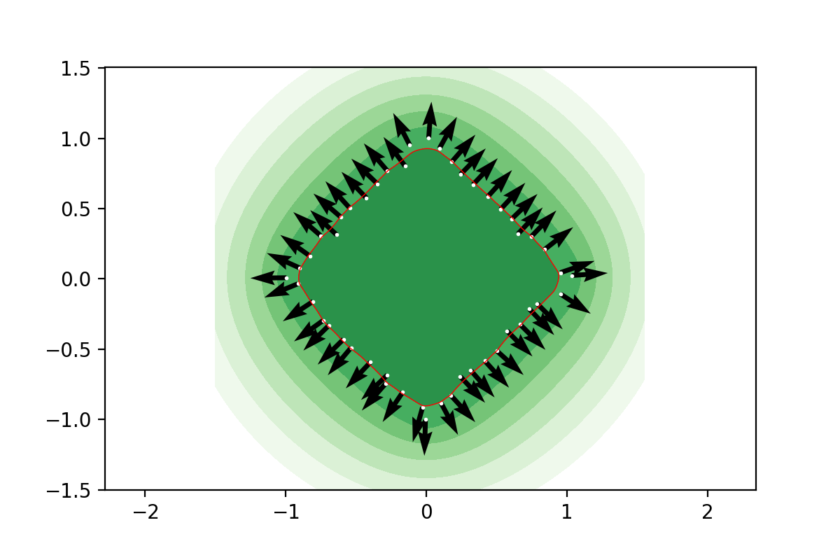
Figure 13. The square example revisited by randomly displacing the original exact sample by 50% noise. Depicted are the level lines and implied normals obtained by means of the Laplace kernel based signature function compute with different regularization levels $\alpha=0,10^{-10},.01,.05,.1,.25$ in increasing order from top left to bottom right.

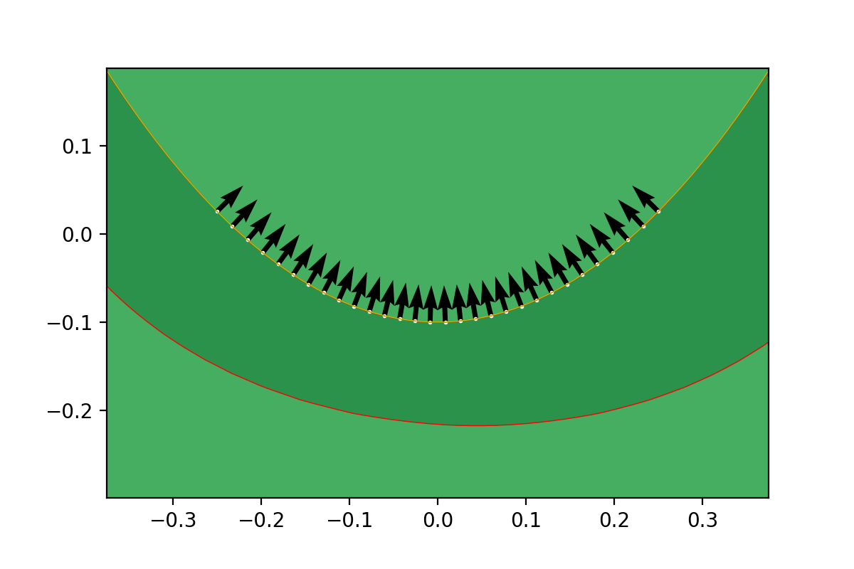
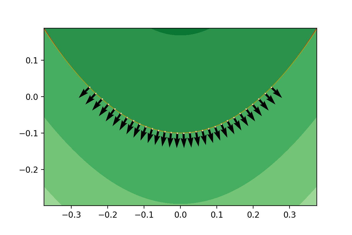
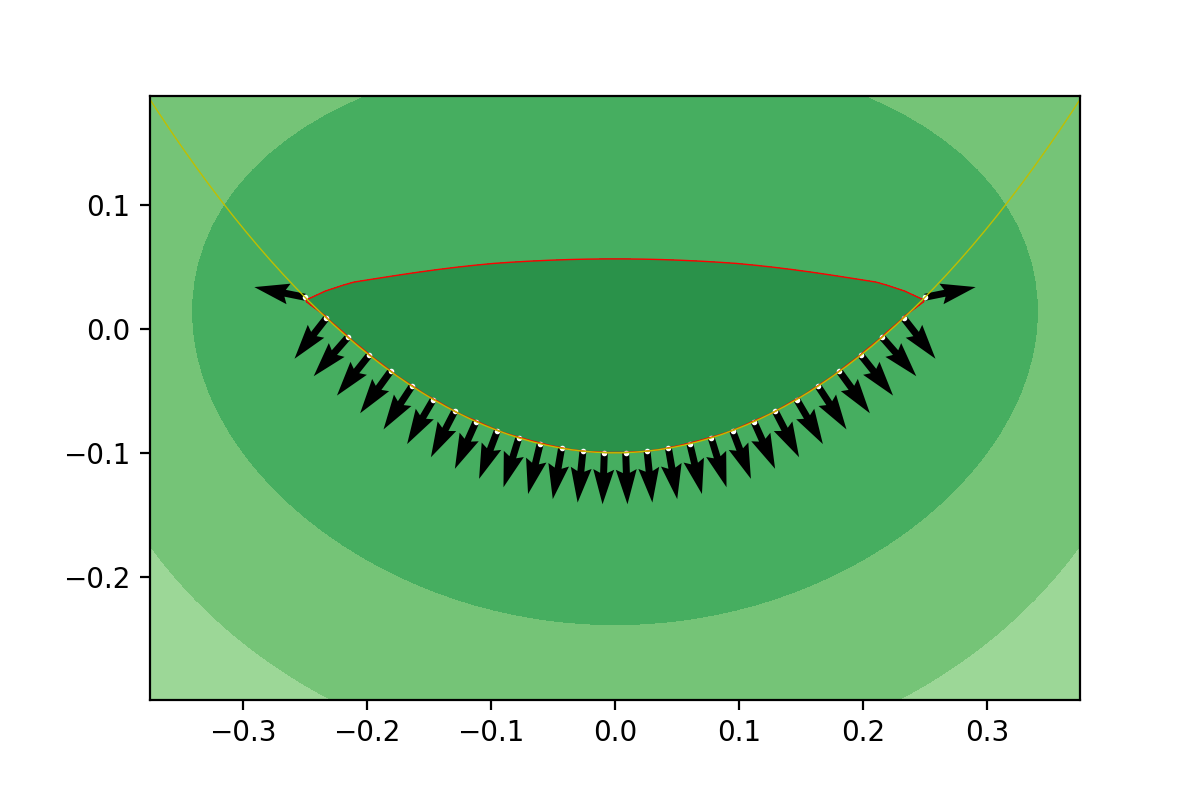
Figure 14. The top row depicts the implied level line (in red) of the signature function of the graph (in yellow) of the function $y=-1+x^{2}+|x|^{2.5}$ for $x\in[-.25,.25]$ along the implied normals (at the data points) obtained using the Gaussian kernel. The second row depicts the same for the Laplace kernel. The experiments in the first column correspond to no regularization ($\alpha=0$), where $\alpha=10^{-10}$ for the ones in the right column.

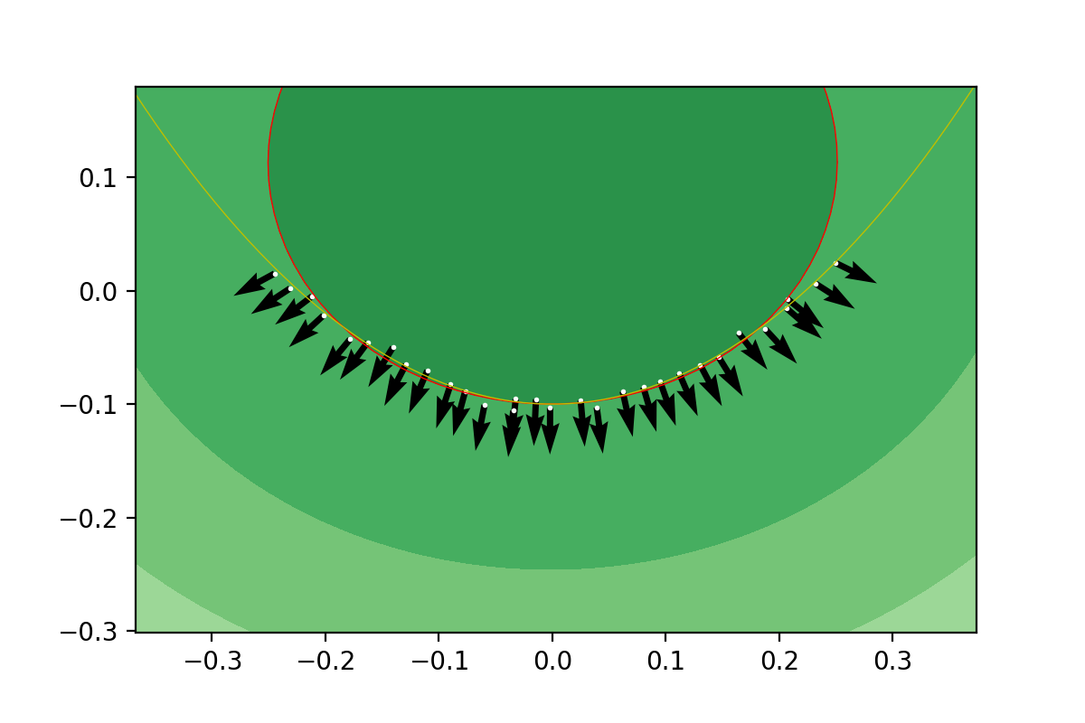
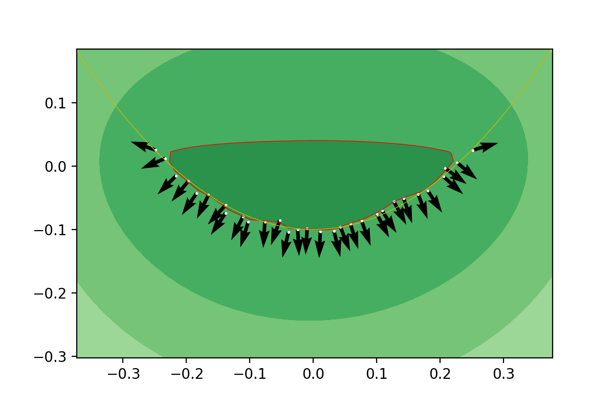
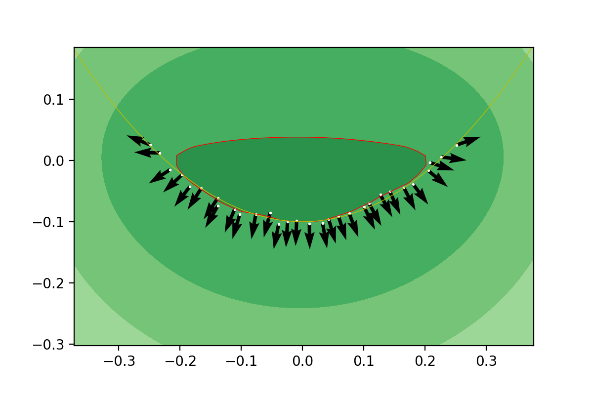
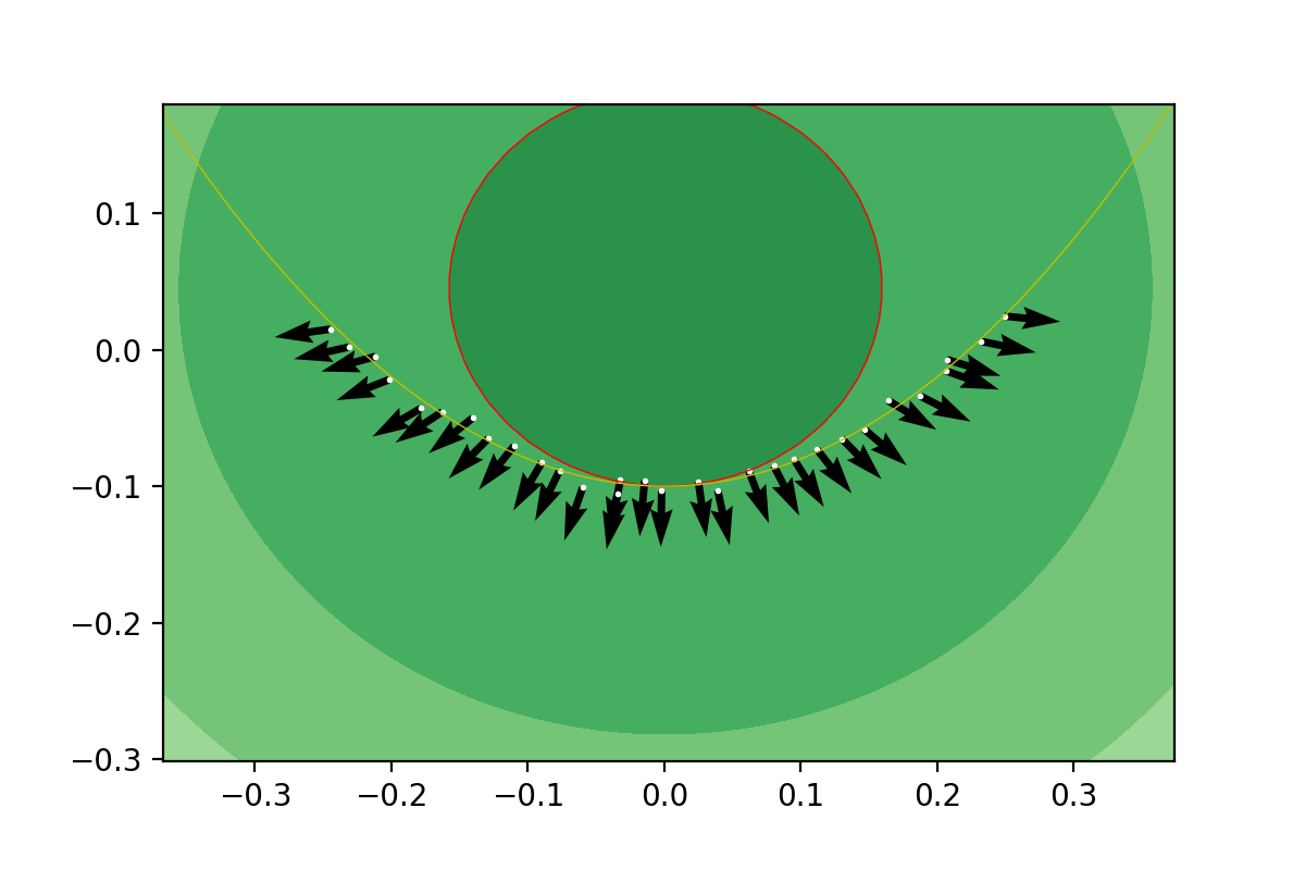
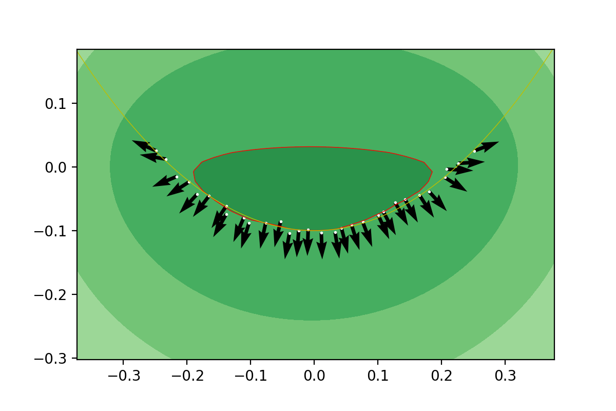
Figure 15. The graph example revisited by randomly displacing the original exact sample by 10% and 50% noise. Depicted are the level lines and implied normals obtained by means of the Gauss (left column) and Laplace (right column) kernel based signature function computed with different regularization levels $\alpha=.01,.05,.1$ in increasing order from top left to bottom right.

Next we consider some examples where $d=3$, starting with the unit sphere. We take a random sample of points of size $m=80$ that lie exactly on the sphere and used them to compute the signature function, which, in turn, we use to obtain the implied curvature at another set of randomly chosen points on the sphere. The random sample is generated by choosing $x_{3}$ uniformly at random from $[-1,1]$ and then setting $x=(\sqrt{1-x_{3}^{2}}\cos(\theta),\sqrt{1-x_{3}^{2}}\sin(\theta),x^{3})$ for $\theta$ uniformly distributed in $[0,2\pi)$. It is depicted in Figure 16.

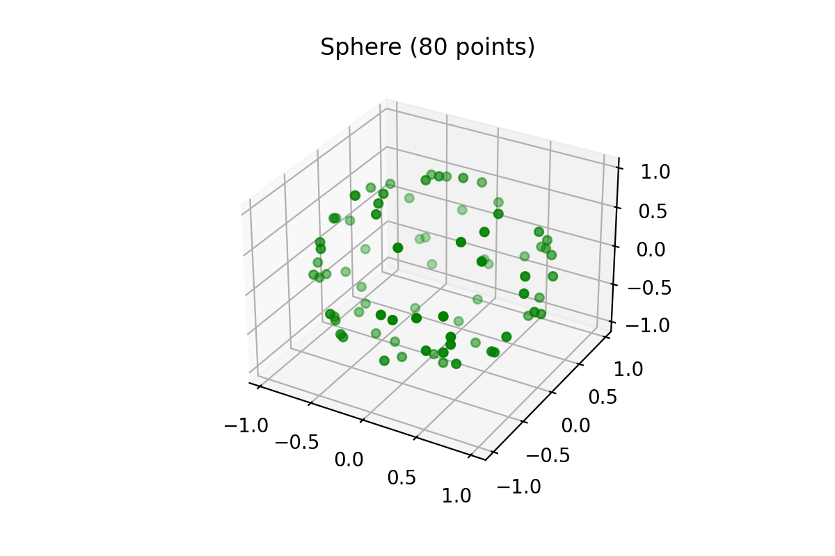
Figure 16. 80 points randomly sampled from the unit sphere.

Then we compute the implied normals and implied curvatures at 32 other points on the sphere sampled in the same way. The maximum deviation from the value 1 of the signature function at these points is $.0000225$, the maximum angle between the exact normal and the implied normal is $0.00873$ degrees, and the maximum error in curvature is $0.0143$. Finally we consider a higher codimension manifold. A portion of the spiral given by the parametrization

$$X:[0,1]\to\mathbb{R}^{3},\>t\mapsto\bigl{(}\cos(2\pi t),\sin(2\pi t),t\bigr{)}.$$

It has constant curvature $\kappa=\frac{4\pi^{2}}{4\pi^{2}+1}\simeq 0.97529$. In this case the method delivers a hypersurface that contains the spiral. One of the principal curvatures of this hypersurafce does approximate the curvature of the spiral but the other is spurious. It is, however, possible to use both kernels, which lead to distinct hypersurfaces containing the spiral and which happen to have significantly different spurious principal curvatures. Table 4 shows the implied curvatures ($\alpha=10^{-10}$) of the hypersurfaces generated with the two different kernels based on 256 points equally spaced along the spiral. These are computed about the midpoint of the spiral (the midpoint itself and the two neighbors on each side), where the accuracy is expected to be best. The “real” curvature can clearly be identified. Notice that we change the Laplace kernel in this calculation by setting the regularization parameter to $r=1$ in order for it to yield good approximations for the curvatures. The use of different kernels can also be used in order to estimate the dimension of geometrical object given a sample of its points. To illustrate this, we consider a spiral in $\mathbb{R}^{5}$ given by

$$X:[0,1]\to\mathbb{R}^{5},\>t\mapsto\bigl{(}\cos(2\pi t),\sin(2\pi t),t,t,t\bigr{)},$$

the curvature of which amounts to $\kappa=\frac{4\pi^{2}}{4\pi^{2}+3}\simeq.9294$. By comparing the curvatures computed using the two different kernels based on a sample of 256 points equally spaced along the curve, shown in Table 5, it is apparent that only one curvature remains “unchanged” when switching the kernel, pointing to the “correct” curvature and the one dimensionality of the point cloud.

Kernel/$|$Curvature$|$
Gauss (approximate)	0.9678	0.9742	0.9742	0.9742	0.9742
Laplace (approximate)	0.9752	0.9753	0.9753	0.9752	0.9752
Gauss (spurious)	3.1960	3.1965	3.1968	3.1968	3.1965
Laplace (spurious)	1.7175	1.7176	1.7177	1.7177	1.7176

Table 4. Absolute value of the implied curvature at points located in the center of the spiral in $\mathbb{R}^{3}$.

Kernel/$|$Curvature$|$
Gauss (approximate)	0.9468	0.9468	0.9468	0.9468	0.9468
Laplace (approximate)	0.9513	0.9514	0.9514	0.9513	0.9513
Gauss (spurious 1)	3.3624	3.3625	3.3625	3.3624	3.3621
Laplace (spurious 1)	1.7190	1.7191	1.7191	1.7190	1.7189
Gauss (spurious 2)	3.2080	3.2083	3.2083	3.2080	3.2073
Laplace (spurious 2)	1.5909	1.5910	1.5910	1.5909	1.5907
Gauss (spurious 3)	3.3624	3.3625	3.3625	3.3624	3.3621
Laplace (spurious 3)	1.7190	1.7191	1.7191	1.7190	1.7189

Table 5. Absolute value of the implied curvature at points located in the center of the spiral in $\mathbb{R}^{5}$.

References

- [1] P. Guidotti. Dimension Independent Data Sets Approximation and Applications to Classification. Advanced Modeling and Simulation in Engineering Sciences, 11(1), 2024.
- [2] H. Wendland. Scattered Data Approximations. Number 17 in Cambridge Monographs on Applied and Computational Mathematics. Cambridge University Press, Cambridge, 2004.