Loss-based prior for tree topologies in BART models

Abstract

We present a novel prior for tree topology within Bayesian Additive Regression Trees (BART) models. This approach quantifies the hypothetical loss in information and the loss due to complexity associated with choosing the “wrong” tree structure. The resulting prior distribution is compellingly geared toward sparsity—a critical feature considering BART models’ tendency to overfit. Our method incorporates prior knowledge into the distribution via two parameters that govern the tree’s depth and balance between its left and right branches. Additionally, we propose a default calibration for these parameters, offering an objective version of the prior. We demonstrate our method’s efficacy on both simulated and real datasets.

Keywords BART, Objective Bayes, Loss-based prior, Bayesian Machine learning.

1 Introduction

Bayesian additive regression trees (BART) introduced by Chipman et al. (2006, 2010) are a flexible class of semi-parametric models for regression and classification problems in the presence of a high number of covariates. The main objective of BART is to model an unknown function linking the covariates to the observations as a sum of binary regression trees (Breiman, 2017). They are a generalisation of the classification and regression tree (CART) models in which only one binary regression tree is considered (Chipman et al., 1998; Denison et al., 1998). BART models were firstly introduced for regression problems with Gaussian errors and multicategory classification problems but since then they have been generalised to multinomial and multinomial logit models (Murray, 2017), gaussian models where also the variance depends on covariates (Pratola et al., 2020), count data (Murray, 2017), gamma regression models (Linero et al., 2020), and to Poisson processes (Lamprinakou et al., 2023). They also have been adapted to face different problems such as variable selection (Linero, 2018), regression with monotonicity constraints (Chipman et al., 2022), survival analysis (Bonato et al., 2011; Sparapani et al., 2016), and causal inference (Hill, 2011; Hahn et al., 2020) just to name a few. Furthermore, much effort has been devoted building a theoretical framework for BART in order to study posterior convergence (Rocková and van der Pas, 2017; Ročková and Saha, 2019; Rocková, 2019; Jeong and Rockova, 2023). We refer to Hill et al. (2020) for a nice introduction to the BART models and their applications.

One characteristic of BART and CART models is that the prior on the tree space acts as a regularisation prior. Specifically, the prior is defined by specifying a distribution on binary tree space and the splitting rules at the internal nodes, and a conditional distribution on the value at the terminal nodes. The prior on the tree space is used to downweight undesirable trees according to specific characteristics such as tree complexity (e.g. number of terminal nodes, depth). This is because, especially in BART models, we want to avoid situations in which one tree is unduly influencial and to advantage cases where each tree captures a specific aspect of the data. The most used tree prior is the one proposed by (Chipman et al., 1998) which specifies, for each node, the probability that the node is a split as a decreasing function of the node’s depth, and the tree prior is the product of the nodes’ probabilities. We refer to this prior as the classic tree prior (CL) as it is the most used in practice. While intuitively appealing, using this prior is relative difficult to incorporate prior information on the number of terminal nodes. Denison et al. (1998) proposed another way by directly specifying a distribution on the number of terminal nodes and a uniform distribution over the trees with a given number of terminal nodes. However, this prior tends to concentrate around skewed trees with a large difference between terminal nodes on the left and right branch. Wu et al. (2007) proposed the pinball prior in which they tried to mix these approaches by considering a prior on the number of terminal nodes and cascading down from the top of tree specifying a probability on the number of terminal nodes going left and right. This gives control over the shape of tree being more or less skewed. Other examples that tries to overcome the problem are the spike-and-tree (Rocková and van der Pas, 2017) and the Dirichlet prior proposed by Linero (2018) which both penalise the complexity of the tree by specifying a sparse prior on the predictors space. For all the priors mentioned above the choice of parameters is subjective and researchers usually rely on default values which lack a mathematical and objective motivation.

A way to design an objective prior distribution is the loss-based prior approach developed by Villa and Walker (2015b). This is based on considering the prior for a tree to be proportional to a function of the loss that one would incur by selecting a different tree than the one generating the data. The loss is considered both in terms of information and in terms of complexity. The prior obtained with this approach is appealing for BART and CART models because it authomatically penalises for the complexity of the tree. Furthermore, the parameters of the prior distribution can be chosen by maximising the expected loss and therefore they are both mathematically justified and objective. The loss-based approach has been used to design objective priors in a variety of contexts: for the parameters of a standard, skewed and multivariate $t$-distribution (Villa and Walker, 2014; Leisen et al., 2017; Villa and Rubio, 2018), for discrete parameters spaces (Villa and Walker, 2015a), for time series analysis (Leisen et al., 2020), for change-point analysis (Hinoveanu et al., 2019), for the number of components in a mixture model (Grazian et al., 2020), for variable selection in linear regression (Villa and Lee, 2020), and for Gaussian grapichal models (Hinoveanu et al., 2020).

In this article, we apply the loss-based approach to design an objective prior distribution for the tree structure in BART and CART models. The prior we propose penalises for the number of terminal nodes and for the difference between the number of terminal nodes on the left and right branch (used as a measure of skeweness) favouring more balanced trees. This is similar in spirit to the pinball prior but presents multiple advantages. First of all, the prior has a clear and sound mathematical justification being based on a definition of loss in complexity and in information. This allows us to calibrate the parameters of the prior by maximizing the expected loss and provide an objective way to determine a default distribution in absence of prior knowledge. In the case where there is prior knowledge, we provide the analytical expression of the distribution of the number of terminal nodes and the difference between left and right terminal nodes, in contrast to approaches like Chipman et al. (1998) where these can be accessed only through simulations, and therefore is easier to find the value of the parameters by specifying the quantiles of the distributions. We have compared the performance of our prior against the prior proposed by (Chipman et al., 1998) on a simulated gaussian regression problem and real data classification problem. In both cases, we found that the loss-based prior with parameters calibrated via expected loss maximisation is the one providing the best results. Here, for best results we mean, in the simulated case, that the posterior distribution of the number of terminal nodes and depth is more concentrated around the true value. In the real data case, we mean that, under the loss based prior, during the MCMC search we visit shorter trees without losing out in terms of likelihood or missing rate. This can be particularly relevant for BART and CART models, and in any context in which the interest lies in avoiding unnecessarly complex trees.

The prior we propose in this article has some other useful features. Computationally, the loss-based prior needs only the number of terminal nodes and the difference between left and right terminal nodes which, for each MCMC sample, can be calculated knowing the previous tree in the chain. This property can be leveraged to design faster MCMC algorithms. Theoretically, the loss-based prior approach could be used to design a prior on the number of trees in a BART model, a quantity for which there is currently no prior distribution and is considered to be a tuning parameter (the default and most commonly used value is 200). This is problematic both because it would be interesting to be able to estimate this quantity from the data, to make inference on it, and because this choice is subjective, it is more a precautionary measure (it is better to consider more trees than necessary rather than less) that works well than something justified. Having a unified approach to design both the prior on the tree structure and the number of trees in the model would enable new lines of research, and add flexibility to previous models.

The paper is organised as follow: Section 2 introduces formally the BART model, the prior proposed by (Chipman et al., 1998) for the tree structure and the loss-based approach. Section 3 describes the prior on the tree structure obtained using the loss-based approach. Section 4 describes the MCMC algorithm used to explore the posterior distribution. Section 5 compares the performance of the CL prior with the loss-based prior obtained in Section 3 on simulated data. The comparison includes instances of the loss-based prior replicating the default CL prior, and vice versa. Section 6 compares the performance of the default classic prior and the default loss-based prior on the breast cancer data analysed in Chipman et al. (1998) and Wu et al. (2007). Finally, in Section 7 we discuss the results shown in the article and draw some conclusions.

2 Preliminaries on BART and loss-based approach

In this Section, we set up the notation used through the paper, give a formal description of the BART model, the CL prior proposed by Chipman et al. (1998), and the loss-based prior approach that is used in Section 3 to design an objective prior on the tree structure.

2.1 BART models

The Bayesian Additive Regression Trees model (BART, Chipman et al., 2010) is a way of making inference about an unknown function $f(\bm{x})$ that predicts an output $Y$ such that

$$Y=f(\bm{x})+\epsilon,\quad\quad\epsilon\sim N(0,\sigma^{2}),$$ (1)

where $\bm{x}=(x_{1},\dots,x_{p})$ is a p-dimensional vector of covariates, usually assumed to be $\bm{x}\in[0,1]^{p}$. The function $f(\cdot)$ is unknown and assumed to be smooth.

The aim of the BART model is to make inference on the function $f(\cdot)$ and the idea is to approximate $f(\cdot)$ using a sum of $m\geq 1$ regression trees so that

$$Y=\sum_{j=1}^{m}g(\bm{x},T_{j},M_{j})+\epsilon\quad\quad\epsilon\sim N(0,\sigma^{2}),$$ (2)

where $T_{j}$ is a binary tree composed by splitting rules of the kind $x_{i}\leq\tau$ at each internal node, $M_{j}=(\mu_{1},\dots,\mu_{n_{L}(T_{j})})$ contains the values at the terminal nodes, $n_{L}(T_{j})$ is the number of terminal nodes, and $g(\bm{x},T_{j},M_{j})$ represents the $j$-th regression tree.

Essentially, a regression tree is a way to represent a piecewise constant function on a partition. The internal nodes of the tree represent the partition, the terminal nodes represent the different elements of the partition, and the value at the terminal nodes represents the value assumed by the function on the corresponding element of the partition. However, regression trees are not capable of representing any partition, but only partitions composed by non-overlapping rectangles. In other words, we are interested in partitions obtained by nested parallel-axis splits.

Each internal node is equipped with a splitting rule on one of the predictor directions of the form $x_{i}\leq\tau$ for $i=1,...,p$. So, a splitting rule is composed by a splitting variable $i$ and splitting value $\tau$. The value $\tau$ is chosen to be one of the observed values $x_{ij}$ with $j=1,...,n$ ($n$, number of observations), or chosen uniformly in a range of values $(x_{il},x_{iu})$. If the observation meets the splitting rule than we move on the left branch of the tree, and we move on the right branch otherwise. In this way, each observation is associated with a terminal node of the tree. Therefore, the values at the terminal nodes depend on which observations are associated with each terminal node.

In order to be able to estimate the values at the terminal nodes we are mostly interested in partitions with at least one (or $n_{\mu}$) observations associated with each terminal node. Chipman et al. (1998) calls these partitions valid and this property depends on the data at hand. For example, if we have $n$ observations and we want at least one observations per terminal node, then, the maximum number of terminal node of a valid tree is $n$. A more formal definition can be given by starting from the notion of cell size. The cell size is:

Definition 1 (Cell Size)

Given a partition $\bm{\Omega}=\{\Omega_{k}\}_{k=1}^{N}$ of $\mathcal{X}=[0,1]^{p}$, and a set of observations $\bm{x}_{1},...,\bm{x}_{n}$ such that $\bm{x}_{i}\in\mathcal{X}$ for each $i=1,...,n$, the cell size $S(\Omega_{k})$ of $\Omega_{k}$ is the fraction of observations falling in $\Omega_{k}$, namely

$$S(\Omega_{k})=\frac{1}{n}\sum_{j=1}^{n}\mathbb{I}(\bm{x}_{j}\in\Omega_{k})$$ (3)

where $\mathbb{I}(\bm{x}\in\Omega_{k})$ is an indicator function assuming the value 1 if the condition is met and 0 otherwise.

Then, we can define a valid partition as

Definition 2 (Valid Partition)

Given a partition $\bm{\Omega}=\{\Omega_{k}\}_{k=1}^{N}$ of $\mathcal{X}=[0,1]^{p}$, and a set of observations $\bm{x}_{1},...,\bm{x}_{n}$ such that $\bm{x}_{i}\in\mathcal{X}$ for each $i=1,...,n$, the partition is valid if

$$S(\Omega_{k})\geq\frac{C^{2}}{n},\quad\emph{for any }k=1,...,N$$ (4)

for a constant $C^{2}\geq 1$.

A tree that induces a valid partition is called a valid tree. From now on, we will only focus on valid trees (partitions).

2.2 Priors for BART

Any bayesian analysis requires a prior distribution to be defined on the parameters of the model. For a single tree regression models, this means that we need to define a prior on the tree topology (the shape of the tree), the splitting rules, the values at the terminal nodes and the marginal variance. These priors are usually assumed to be independent (Chipman et al., 1998) so the prior for the whole set of parameters is the product of the prior on the tree topology, the prior on the splitting rules, the prior on the values at the terminal nodes and the prior on the marginal variance. Given that in this article we provide a new prior for the tree topology, in this section we will describe only this prior. Furthermore, we will specify the prior for one tree; the same prior is used for all the trees in the BART model formulation reported in Equation 2. We will assume through out the paper that the prior on the splitting rules, the values at the terminal nodes, and the marginal variance, are the same as described in Chipman et al. (1998) and Chipman et al. (2010).

In BART models, the prior on the tree topology plays the role of a regularisation prior. By regularisation prior, we mean that the prior acts as a penalty on the tree complexity. This is needed in order to avoid overfitting and to keep the relative contribution of each tree to the summation small. If the prior does not penalise for complexity, there is a high probability of having a complex and rich first tree and all the others having a negligible contribution to the summation. This limits interpretability and increase the chances of overfitting.

The most widely used regularisation prior for the tree topology is the one proposed by Chipman et al. (1998) originally proposed for a BART model with a single regression tree ($m=1$). Through out this article, we will refer to this prior as the classic tree prior (CL). The CL prior is defined by providing for each internal node the probability that the node is a split. For a node at depth $d$ (the minimum number of steps from the root to the node) the probability that the node is a split is given by

$$\alpha(1+d)^{-\beta},\quad\alpha\in(0,1),\beta\geq 0$$ (5)

Given a tree $T$ with internal nodes index set $a(T)$ and terminal nodes index set $b(T)$ the CL prior for tree $T$ is then given by

$$\pi_{C}(T)=\prod_{i\in a(T)}\alpha(1+d_{i})^{-\beta}\prod_{j\in b(T)}\left(1-\alpha(1+d_{j})^{-\beta}\right)$$ (6)

The CL prior penalises for complexity assuming that the probability that a node is a split decreases with the depth of the tree. The prior is governed by two parameters $\alpha$ and $\beta$. Parameter $\alpha$ corresponds to the probability that the first node is a split (the first node has depth 0). Parameter $\beta$ regulates how fast the probability that a node is a split decays as a function of the depth of the node. The default setting used in applications (Hill, 2011; Zhang et al., 2020; Sparapani et al., 2020) and in R-packages for BART models such as dbarts (Dorie et al., 2024) are $\alpha=0.95$ and $\beta=2$.

The CL prior formulation induces a distribution on the space of the binary trees which penalises for complexity, in the sense that trees with more terminal nodes, or with terminal nodes at greater depths, are assigned less prior probability. However, retrieving an analytical expression for the distribution on the number of terminal nodes or the depth of the tree (defined as the maximum depth of a node in the tree) is cumbersome. The only way to retrieve the distributions of these quantities is through simulation. Figures 1 and 2 shows the depth and number of terminal nodes distributions for different values of the prior parameters.

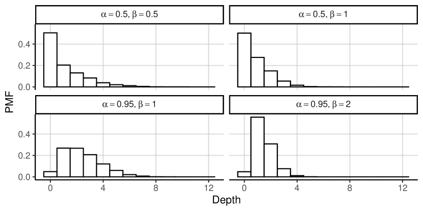
Figure 1: Depth distribution under the CL prior for different combinations of prior parameters $\alpha$ and $\beta$ obtained simulating 10000 trees from the prior.

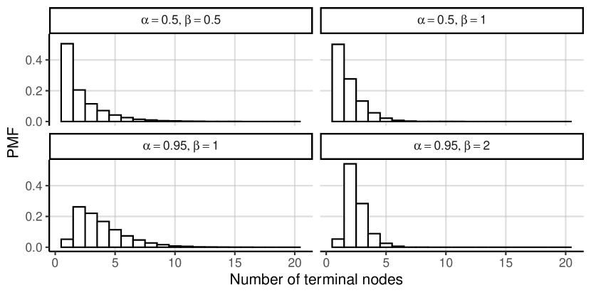
Figure 2: Number of terminal nodes probability mass function under the CL prior for different combinations of prior parameters $\alpha$ and $\beta$ obtained simulating 10000 trees from the prior.

The fact that the distributions of tree-related quantities such as the depth and the number of terminal nodes under the CL prior are obtainable only through simulation is a disadvantage of this prior. Indeed, this makes complicated calibrating the prior parameters by specifying the mean or quantiles of the number of terminal nodes or depth distributions because one have to find the right parameters value by trail and error. Researchers usually starts from the default and then tweek the parameters based on posterior results (Zhang et al., 2020; Hill, 2011). This procedure is inefficient and introduce a degree of subjectivity in the analysis. Instead, this problem vanishes when using our loss-based prior, both because the default parameter values are determined objectively, and because the distribution of the number of terminal nodes is analytically available.

2.3 Loss-based priors

The loss-based approach (Villa and Walker, 2015b) is a technique to design objective prior distributions and has been applied to different problems (Villa and Walker, 2015a; Leisen et al., 2020; Grazian et al., 2020; Hinoveanu et al., 2020). Loss-based priors are based on the idea that the choice of a “wrong” model yields to a loss, which has two components: one is in information and the other is associated to the complexity of the models. The former stems from a well-known Bayesina property (Berk, 1966) that, if a model is misspecified, then the posterior will asymptotically accumulate on the model that is the most similar to the true one, where this similarity is measured in terms of the Kullback-Leibler divergence (KLD Kullback and Leibler, 1951). The latter loss originates from the fact that the more complex a model is, the more of its components have to be considered and measured. Essentially, for a model $\mathcal{M}$ in a family $\mathcal{F}$ we have that

$$\pi(\mathcal{M})\propto\exp\{Loss_{I}(\mathcal{M})+Loss_{C}(\mathcal{M})\}$$ (7)

where $Loss_{I}(\mathcal{M})$ is the loss in information which occurs by selecting a model different from $\mathcal{M}$ when $\mathcal{M}$ is the data-generating model, and $Loss_{C}(\mathcal{M})$ is the loss in complexity incurred by selecting model $\mathcal{M}$. The idea behind this approach is that, models for which we incur a greater loss in information when misspecified should receive more prior probability, and more complex models should be penalised in accordance with a parsimony principle.

The loss in information for a model is considered to be the minimum Kullback-Leibler divergence between the model and the alternative models in a pre-defined family $\mathcal{F}$. For a model $\mathcal{M}$, the greater the minimum KLD distance, the more difficult is to find an alternative model within $\mathcal{F}$ bringing similar information. We assign greater prior distribution to models with higher KLD because we would incur in a greater loss if misspecified.

More formally, given a variable of interest $Y\in\mathcal{Y}$, a set of predictors $\bm{x}\in\mathcal{X}$, and two models $\mathcal{M}$ and $\mathcal{M}^{\prime}$ in $\mathcal{F}$, with distributions $\pi(y|\bm{x})$ and $\pi^{\prime}(y|\bm{x})$, the Kullback-Leibler divergence between the two models is

$$KL(\mathcal{M}||\mathcal{M}^{\prime})=\int_{\mathcal{Y}}\pi(y|\bm{x})\log\left(\frac{\pi(y|\bm{x})}{\pi^{\prime}(y|\bm{x})}\right)dy$$ (8)

and the loss of information is then given by

$$Loss_{I}(M)=\min_{\mathcal{M}^{\prime}\in\mathcal{F}}KL(\mathcal{M}||\mathcal{M}^{\prime})$$ (9)

Contrarily, the loss in complexity strictly depends on the problem at hand and different choices are possible. For example, a natural choice in problems of variable selection is to consider the number of active predictors as loss in complexity (Villa and Lee, 2020). This makes the loss-based prior approach very flexible and it can be tailored to the problem.

3 Loss-based prior for BART

In this Section, we show how to use the loss-based prior approach to design a prior distriution for the tree topology of a BART model. As for the CL prior (see Sec 2.2) the prior is defined for a single tree and applied to all the trees involved in the summation. In this context, the model $\mathcal{M}$ is represented by the tree $T$, the distribution of the observations $\pi(y|\bm{x})$ is the distribution induced by the tree $\pi(y|\bm{x},T,M)=\phi(g(\bm{x},T,M),\sigma^{2})$, where $\phi(a,b)$ is the normal density with mean $a$ and variance $b$, and the family $\mathcal{F}$ is the set of binary trees. We will discuss separately the loss in information, the loss in complexity and the resulting prior.

3.1 Loss in information

The KLD between two trees $T$ and $T^{\prime}$ is given by

$$KL(T||T^{\prime}|\bm{x},M,M^{\prime})=\int_{\mathcal{Y}}\pi(y|\bm{x},T,M)\log\left(\frac{\pi(y|\bm{x},T,M)}{\pi(y|\bm{x},T^{\prime},M^{\prime})}\right)dy,$$ (10)

and the loss in information is given by

$$Loss_{I}(T)=\min_{T^{\prime},M^{\prime}}KL(T||T^{\prime}|\bm{x},M,M^{\prime}).$$ (11)

The KLD is zero when it is possible to find a tree $T^{\prime}$ with terminal node values $M^{\prime}$ that replicates exactly $T$ and $M$. In other words, if we can find $T^{\prime},M^{\prime}$ such that $g(\bm{x},T,M)=g(\bm{x},T^{\prime},M^{\prime})$ for each $\bm{x}$, then the KLD is zero and there is no loss in information in misspecifying the model. This is similar to having nested models where the more complex model replicates the simpler ones. Without considering any limitation on the tree complexity (e.g. maximum number of terminal nodes, maximum depth, etc) it is always possible to find a tree $T^{\prime}\neq T$ with terminal nodes values $M^{\prime}$ that replicates $T,M$. Indeed, it is sufficient to consider $T^{\prime}$ to be obtained by splitting one terminal node (say $j$, with terminal node value $\mu_{j}$) of $T$ to obtain two additional terminal nodes in $T^{\prime}$ with values $\mu^{\prime}_{j},\mu^{\prime}_{j+1}$ and to set $\mu_{j}=\mu^{\prime}_{j}=\mu^{\prime}_{j+1}$. Therefore, with no limitations on the tree topology the KLD is always zero (as well as the loss in information).

Appendix A shows the KLD in the case where there is a maximum number of nodes. In this case, it turns out that the KLD depends on the values at the terminal nodes. Assuming the values at the terminal nodes are i.i.d. then the average KLD over the terminal nodes’ distribution is zero. Without averaging over the distribution of the values at the terminal nodes, considering the KLD will affect mostly the prior for the tree with the maximum number of nodes. Intuitively, this is because, we can assume that each tree, except the most complex one, is nested into a more complex tree. Given that the outer tree will contain at least the same amount of information as the inner one (as it carries more uncertainty), the loss in information will be zero for any tree except the one with the maximum terminal nodes for which the difference is negligible. For this reason, we will consider the loss in information to be equal zero for the remainder of the paper.

3.2 Loss in complexity

We have decided to base the loss in complexity of using tree $T$ on the number of terminal nodes of $T$, namely $n_{L}(T)$, and the difference between the left and right terminal nodes, $\Delta(T)$, where for left (right) terminal nodes we intend the terminal nodes of the left (right) branch of the tree. The number of terminal nodes is a natural measure of complexity for trees (Denison et al., 1998; Wu et al., 2007), while the difference between the number of left and right terminal nodes is included to have control over the skeweness of the tree for a given number of terminal nodes. The loss in complexity is then given by

$$Loss_{C}(T)=-\omega n_{L}(T)-\gamma\Delta(T)$$ (12)

where $\omega\leq 0$ and $\gamma\in\mathbb{R}$ are weights and will be the parameters of the prior. The loss in complexity is negatively oriented meaning that less complex models have loss in complexity closer to zero.

The parameter $\gamma$ is allowed to be negative. Indeed, $\gamma>0$ means that, given the number of terminal nodes, the prior favours trees with an equal number of terminal nodes on the left and right branch. This leads to shallower trees than when $\gamma<0$. On the other hand, when $\gamma<0$ the prior favours trees where the majority of the nodes lies on one of the branches. This induces deeper trees than when $\gamma>0$. In this work, we will consider only cases where $\gamma>0$ which provides a stricter penalty for complexity, however the proposed prior works also for $\gamma<0$, in case there is past evidence that the number of terminal nodes on the left and right branches should be different.

3.3 The prior distribution for the BART model

Considering the expressions given by Equations 11 and 12 for the loss in information and complexity (respectively), the loss-based prior for a tree topology $T$ is given by

$$\pi(T)\propto\exp\{-\omega n_{L}(T)-\gamma\Delta(T)\}$$ (13)

In order to find the normalising constant we consider the following factorisation where, for simplicity, we have dropped the dependence on $T$ of $n_{L}(T)$ and $\Delta(T)$,

$$\pi(T)=\frac{\pi(n_{L})\pi(\Delta|n_{L})}{\mathcal{N}(n_{L},\Delta)}$$ (14)

where $\mathcal{N}(n_{L},\Delta)$ is the number of binary trees with $n_{L}$ terminal nodes and difference between left and right terminal nodes $\Delta$. The analytical expression of $\mathcal{N}(n_{L},\Delta)$ is given in Appendix B. This is equivalent to consider $\pi(n_{L})$ for the number of terminal nodes, $\pi(\Delta|n_{L})$ for the left and right difference given the number of terminal nodes, and a uniform distribution on the trees with the same $n_{L}$ and $\Delta$.

Combining Equations 13 and 14 we have that $\pi(n_{L})$ and $\pi(\Delta|n_{L})$ are

$$\pi(n_{L})\propto e^{-\omega n_{L}},\quad\pi(\Delta|n_{L})\propto e^{-\gamma\Delta}$$ (15)

from which we can calculate the normalising constants for both distributions.

The calculations for the distribution on the number of terminal nodes (assuming no constraints on the maximum number of terminal nodes) are trivial and give

$$\pi(n_{L})=\frac{e^{-\omega n_{L}}}{\sum_{n=1}^{\infty}e^{-\omega n}}=e^{-\omega n_{L}}(e^{\omega}-1)$$ (16)

which is a Geometric distribution with parameter $p=1-e^{-\omega}$ (see Appendix C).

The calculations for the conditional distribution of $\Delta$ given $n_{L}$ are more complicated and we report them explicitly. The conditional distribution is given by

$$\pi(\Delta|n_{L})=\frac{e^{-\gamma\Delta}}{\mathcal{C}(n_{L})}$$ (17)

where $\mathcal{C}(n_{L})$ is the normalising constant which depends on the value of $n_{L}$. To calculate $\mathcal{C}(n_{L})$, we start by observing that if $n_{L}$ is odd then $\Delta$ is also odd (as the difference between an odd and an even number), and, symmetrically, if $n_{L}$ is even, $\Delta$ is even. Furthermore, we consider that $\Delta$ will always be comprised between $0$ and $n_{L}-2$ (as we can have at most $n_{L}-1$ nodes on one side). This implies that the normalising constant $\mathcal{C}(n_{L})$ for the conditional distribution $\pi(\Delta|n_{L})$ must be calculated differently depending on $n_{L}$ being odd or even, and we need to sum over only the odd or even numbers respectively. Therefore, it is useful to consider a change of variable and use $k=\lfloor\Delta/2\rfloor$ (where $\lfloor x\rfloor$ is the maximum integer smaller than $x$) instead of $\Delta$ so that

$$\mathcal{C}(n_{L})=\begin{cases}\sum\limits_{k=0}^{\lfloor\frac{n_{L}-2}{2}\rfloor}e^{-\gamma(2k+1)}=\frac{e^{\gamma}(1-e^{-\gamma(n_{L}-1)})}{e^{2\gamma}-1}&\text{if }n_{L}\text{ odd}\\ \\ \sum\limits_{k=0}^{\lfloor\frac{n_{L}-2}{2}\rfloor}e^{-\gamma(2k)}=\frac{e^{2\gamma}(1-e^{-\gamma n_{L}})}{e^{2\gamma}-1}&\text{if }n_{L}\text{ even}\end{cases}$$ (18)

Equation 18 can be rewritten by considering an indicator function $\delta_{o}(n_{L})$ which is equal to 1 when $n_{L}$ is odd and 0 when $n_{L}$ is even. The equation becomes

$$C(n_{L})=\frac{\delta_{o}(n_{L})(e^{-\gamma}-1)+1-e^{-\gamma n_{L}}}{1-e^{-2\gamma}}$$ (19)

From Equation 19 it is clear that the distribution is not proper for $\gamma=0$ which, indeed, correspond to the uniform case.

To conclude, the loss-based prior for the tree $T$ is given by

$$\pi(T)=\frac{1}{\mathcal{N}(n_{L},\Delta)}e^{-\omega n_{L}}(e^{\omega}-1)\frac{e^{-\gamma\Delta}}{\mathcal{C}(n_{L})}$$ (20)

with $\mathcal{C}(n_{L})$ given by Equation 19.

3.4 Parameter calibration

In this section, we show the tree depth distribution induced by different parameters of the loss-based prior, and we provide a ways to find the values of the parameters to be used as default. This is achieved by maximizing the expected loss.

Figures 3 and 4 show the depth probability mass function and cumulative distribution for different values of the paramters $\omega$ and $\gamma$. We do not show the distribution of the number of terminal nodes which only depends on $\omega$ and is a Geometric distribution. Regarding the depth distribution, it is strongly influenced by the value of $\omega$ which determines the expected number of terminal nodes. The effect of paramter $\gamma$ is most appreciable from Figure 4. We can see that $\gamma$ mostly influences the tail of distribution, and higher values of $\gamma$ provide lighter tails. The case where $\omega$ and $\gamma$ are zero corresponds to the uniform case on the space of possible binary trees.

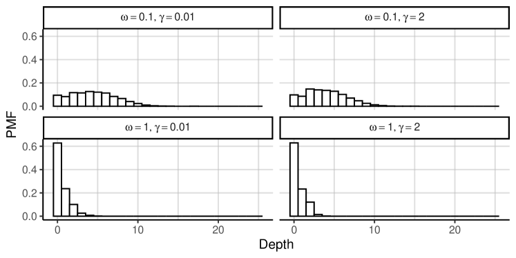
Figure 3: Depth probability mass function induced by the loss-based prior with different values of parameters $\omega$ and $\gamma$, estimated using 10000 tree samples from the prior.

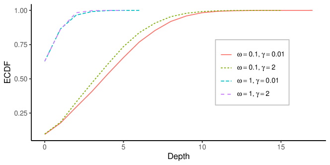
Figure 4: Depth empirical cumulative distribution induced by the loss-based prior with different values of parameters $\omega$ and $\gamma$ (represented by color and line-type), estimated using 10000 tree samples from the prior.

3.4.1 Maximizing the expected Loss

One way to find a default value for the loss-based prior parameters is to set an expression for the expected loss and find the value of the parameters that maximises the expected loss. As expected loss, we consider two alternatives that provides similar results. The two expected losses we consider are

$$E_{L}^{(1)}(\omega,\gamma) =\omega^{2}\mathbb{E}(n_{L})+\gamma\mathbb{E}(\Delta)$$ (21)

$$E_{L}^{(2)}(\omega,\gamma) =\omega^{2}\mathbb{E}(n_{L})+\omega\gamma\mathbb{E}(\Delta)$$ (22)

where $\mathbb{E}(n_{L})$ and $\mathbb{E}(\Delta)$ are the expected values of $n_{L}$ and $\Delta$ with respect to their marginal distributions. We notice that the marginal expected value of $\Delta$ is a function of both $\omega$ and $\gamma$.

Figure 5 shows the expected loss as a function of the parameters using the two expected loss formulations above. The values of the paramters (represented by the black dots) maximizing the expected loss is similar, indeed, we get $\omega^{*}_{1}=1.568$ and $\gamma^{*}_{1}=0.628$ using $E_{L}^{(1)}(\omega,\gamma)$, and $\omega^{*}_{2}=1.561$ and $\gamma^{*}_{2}=0.629$ using $E_{L}^{(2)}(\omega,\gamma)$ as the expected loss function. Given the small difference between the values of the parameters maximizing the expected loss in the two cases, we proceed considering $E_{L}^{(2)}(\omega,\gamma)$ as the expected loss function and $\omega^{*}=\omega^{*}_{2},\gamma^{*}=\gamma^{*}_{2}$ as default values of the parameters. From now on, when we refer to the default loss-based prior, we intend the loss-based prior with parameters $\omega^{*}=1.561$ and $\gamma^{*}=0.629$.

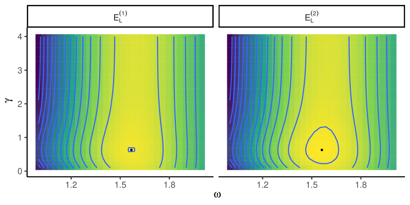
Figure 5: Expected loss as a function of loss-based prior parameters $\omega\in(1,2)$ and $\gamma\in(0,4)$ considering as expected loss the functions $E_{L}^{(1)}(\omega,\gamma)$ (left) and $E_{L}^{(2)}(\omega,\gamma)$ (right). In each panel, the black point represents the values of the parameters maximizing the expected loss in each case.

4 MCMC for BART

In this Section, we describe how to retrieve information on the posterior distribution of the BART model’s parameters which are the $m$ trees $T_{1},...,T_{m}$, the value at the terminal nodes $M_{1},...,M_{m}$, and the marginal variance $\sigma$. This is commonly done using a backfitting Markov-Chain Monte Carlo (MCMC Hastie and Tibshirani, 2000) algorithm introduced by Chipman et al. (1998) for the CART model and extended in Chipman et al. (2010) to the BART model. The MCMC algorithm for BART is based on the idea of recursively using the algorithm for CART to obtain samples fthe $j$-th tree in the summation conditionally on the value of the other trees, the process is repeated for each tree $j=1,...,m$. The MCMC algorithm for CART is a modification of the Metropolis-Hastings (MH) algorithm REF where, in each iteration, a new tree is proposed which is then accepted or rejected. For this reason this section is divided into a first part describing the general MCMC algorithm for BART and a second part describing the MH algorithm for CART.

4.1 Backfitting MCMC for BART

Given a set of observations, $\mathbf{y}=(y_{1},..,y_{n})$, the MCMC algorithm is used to produce samples from the posterior distribution

$$\pi((T_{1},M_{1}),...,(T_{m},M_{m}),\sigma|\mathbf{y}),$$

The backfitting MCMC algorithm is essentially a Gibbs sampler. Each of the $m$ couples $(T_{j},M_{j})$ is sampled conditionally on the other $m-1$. More formally, we call $\mathbf{T}_{-j}$ and $\mathcal{M}_{-j}$ the set of all $m$ trees and terminal nodes values except tree and set $j$. For each MCMC iteration and $(T_{j},M_{j}),j=1,...,m$ a sample from the conditional distribution of

$$(T_{j},M_{j})|\mathbf{T}_{-j},\mathbf{M}_{-j},\mathbf{y},\sigma$$ (23)

is obtained, followed by a sample from

$$\sigma|(T_{1},M_{1}),...,(T_{m},M_{m}),\mathbf{y}.$$ (24)

In order to draw $(T_{j},M_{J})$ from its conditional distribution, it is important to notice that the conditional distribution in Equation 23 depends on $\mathbf{T}_{-j}$, $\mathbf{M}_{-j}$ and $\mathbf{y}$ only through the vector of residuals $\mathbf{R}_{j}=(R_{1j},...,R_{nj})$ where the single component is given by

$$R_{ij}=\mathbf{y}_{i}-\sum_{k\neq j}g(\mathbf{x}_{i},T_{k},M_{k})$$ (25)

So, extracting a sample from Equation 23 is equivalent to sampling the posterior of a single tree model

$$(T_{j},M_{j})|\mathbf{R}_{j},\sigma$$ (26)

where $\mathbf{R}_{j}$ plays the role of the observations.

In this context, if a conjugate prior is used for the terminal node values, the posterior for the tree is given by

$$\pi(T_{j}|\mathbf{R}_{j},\sigma)=\pi(T_{j})\int\pi(\mathbf{R}_{j}|T_{j},M_{j},\sigma)\pi(M_{j}|T_{j},\sigma)dM_{j}$$ (27)

which is available in close form, and we can draw a sample from the posterior distribution of $(T_{j},M_{J})|\mathbf{R}_{j},\sigma$ by sampling a tree from the posterior of

$$T_{j}|\mathbf{R}_{j},\sigma.$$ (28)

This step is performed using the Metropolis-Hastings MCMC algorithm for CART models using $\mathbf{R}_{j}$ as observations. Then, conditionally on the obtained tree, we sample the value at the terminal nodes from

$$M_{j}|T_{j},\mathbf{R}_{j},\sigma.$$ (29)

It is common practice to assume a conjugate prior for the values at the terminal nodes, and therefore, for this step we can sample directly from the conditional posterior distribution. For example, considering the BART model in Equation 2 and assuming a normal prior for the terminal node values, also the posterior distribution is normal.

Lastly, for the marginal variance a conjugate prior is assumed. For example, considering the BART model in Equation 2, if an Inverse-Gamma distribution is chosen as prior for the marginal variance, the posterior of the marginal variance conditional on the values of $(T_{1},M_{1}),...,(T_{m},M_{m})$ it is also an Inverse-Gamma distribution, and therefore we can sample directly from it.

The algorithm for BART can be summarised in steps in Algorithm 1

Algorithm 1 MCMC for BART - $(i+1)$-th iteration

1:Previous step produces $(T_{j}^{(i)},M_{j}^{(i)})$ for $j=1,...,m$, and $\sigma^{(i)}$

2:for j = 1,…,m do

3:     Calculate residuals $\mathbf{R}_{j}^{(i)}$ using Equation 25

4:     Sample $T_{j}^{(i+1)}$ from $T_{j}|\mathbf{R}_{-j}^{(i)},\sigma$ $\triangleright$ Using algorithm for CART

5:     Sample $M_{j}^{(i+1)}$ from $M_{j}|T_{j}^{i+1},\mathbf{R}_{j},\sigma$$\triangleright$ From the conjugate posterior

6:end for

7:Sample $\sigma^{(i+1)}$ from $\sigma|(T_{1}^{(i+1)},M_{1}^{(i+1)}),...,(T_{m}^{(i+1)},M_{m}^{(i+1)}),\mathbf{y}$$\triangleright$ From the conjugate posterior

4.2 Metropolis-Hastings MCMC for CART

In this Section, we describe the Metropolis-Hastings MCMC algorithm (Chipman et al., 1998) used to sample $(T,M)$ from the conditional distribution of $T|\mathbf{y},\sigma$. This algorithm was developed to explore the posterior distribution of the tree of a CART model, which is an instance of the BART model described by Equation 2 considering $m=1$. The goal is to be able to generate samples $T^{(0)},T^{(1)},T^{(2)},\dots$ from the posterior distribution $\pi(T|\mathbf{y},\sigma)$.

At each iteration, the algorithm is based on proposing a new candidate tree $T^{*}$, and accepting/rejecting it based on some probability. At iteration $i+1$, the new tree is proposed by performing a move on the previous tree $T^{(i)}$. Here, we describe the original algorith in which a new tree is proposed according to one of four possible moves (GROW, PRUNE, SWAP, CHANGE). However, we notice that much research has been done in designing alternatives moves that provides better mixing (Wu et al., 2007; Pratola, 2016), but this is beyond the scope of this article.

To generate the tree $T^{*}$ from $T^{(i)}$, we pick at random one of the following possible moves

• GROW: Randomly choose a terminal node and split it into two additional terminal nodes. The new splitting rule is assigned according to the prior.

• PRUNE: Randomly choose a parent of a terminal node and turn it into a terminal node by remove its children.

• SWAP: Randomly choose a parent-child pair of internal nodes and swap their splitting rules.

• CHANGE: Randomly choose an internal node and assign a new splitting rule according to the prior distribution.

The moves are perfomed ensuring that $T^{*}$ yields a valid partition defined in Definition 2 for some $C^{2}\geq 1$. These moves define a transition kernel $q(T,T^{*})$ given by the probability of obtaining $T^{*}$ from $T$. An appealing feature of this kernel is that it produces a reversible Markov chain given that the PRUNE and GROW moves are counterparts, while SWAP and CHANGE are their own counterparts.

Once a tree $T^{*}$ is produced from tree $T^{(i)}$ according to $q(T^{(i)},T^{*})$, it is accepted with probability

$$\alpha(T^{(i)},T^{*})=\min\left(\frac{q(T^{*},T^{(i)})\pi(\mathbf{y}|T^{*})\pi(T^{*})}{q(T^{(i)},T^{*})\pi(\mathbf{y}|T^{(i)})\pi(T^{(i)})},1\right).$$ (30)

Otherwise, the tree does not change.

To summarise, the algorithm to explore the tree posterior of a CART model is given in Algorithm 2

Algorithm 2 MCMC for CART - $(i+1)$-th iteration

1:The previous step produces $T^{(i)}$

2:Generate $T^{*}\sim q(T^{(i)},T^{*})$

3:Compute acceptance probability $\alpha(T^{(i)},T^{*})$ according to Equation 30

4:Set $T^{(i+1)}=T^{*}$ with probability $\alpha(T^{(i)},T^{*})$, or $T^{(i+1)}=T^{(i)}$ otherwise

5 Simulation Study

In this section, we simulate observations from a known CART model and we compare the posterior distributions obtained using different instances of the loss-based and CL prior. The choice of using a CART model, which is a case of BART model with $m=1$, is motivated by the fact that the MCMC algorithm described in the previous section is influenced by the prior only when computing the acceptance probabilities in the MCMC for CART. Therfore, it is appropriate to compare the performance of the two priors in this simplified scenario without loss of generality.

We focus on the posterior distribution of the number of terminal nodes and the depth of the tree. These posterior distributions are estimated running the MCMC algorithm described in Section 4. We consider the marginal variance $\sigma^{2}$ as known, while for the splitting rules we consider a prior distribution given by assuming a discrete uniform distribution on the space of available predictors for the splitting variable and a continuous uniform distribution between a range of available values for the splitting value. The choice of prior distribution for the splitting rule does not change qualitatively the results shown in this section given that only the tree prior is changing between models. For each model, we run 100 chains in parallel, each chain has 500 iterations. The posterior distributions are obtained considering a born-in of 250 observations per chain.

We simulate 300 observations according to a single tree model ($m=1$) considering 3 available predictors $X_{1},X_{2},X_{3}$ distributed according to

$$X_{1j} \sim\begin{cases}\text{Unif}(0.1,0.4)&j=1,\dots,200\\ \text{Unif}(0.6,0.9)&j=201,\dots,300\end{cases}$$

$$X_{2j} \sim\begin{cases}\text{Unif}(0.1,0.4)&j=1,\dots,100\\ \text{Unif}(0.6,0.9)&j=101,\dots,200\\ \text{Unif}(0.1,0.9)&j=201,\dots,300\end{cases}$$ (31)

$$X_{3j} \sim\begin{cases}\text{Unif}(0.6,0.9)&j=1,\dots,200\\ \text{Unif}(0.1,0.4)&j=201,\dots,300\end{cases}$$

and observations given by

$$Y_{j}=\begin{cases}1+N(0,0.25)&\text{if }X_{1j}\leq 0.5,X_{2j}\leq 0.5\\ 3+N(0,0.25)&\text{if }X_{1j}\leq 0.5,X_{2j}>0.5\\ 5+N(0,0.25)&\text{if }X_{1j}>0.5\end{cases}$$ (32)

We assume the model described by Equation 32 is the same as the model in Equation 2 with $m=1$ and considers one regression tree $T$, given by the top-left panel of Figure 6. The marginal variance is $\sigma^{2}=0.25$. This is the same model used by Wu et al. (2007) in their simulation experiment. In this model, only predictors $X_{1}$ and $X_{2}$ are actually used to generate $Y$, while $X_{3}$ is there as a disturbance term. Figure 6 shows scatter plots of $Y$ against $X_{1},X_{2},X_{3}$.

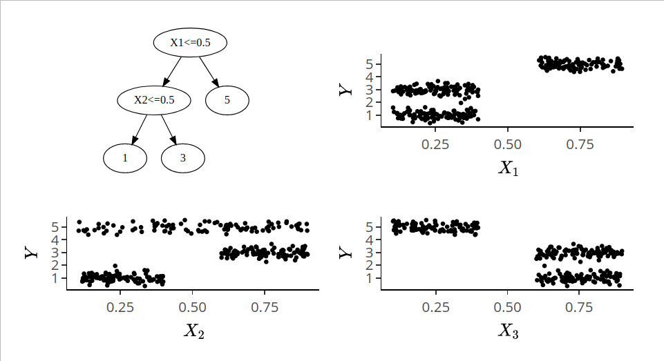
Figure 6: Tree and scatter plots of 300 observations taken from the model specified in Equation 32.

We consider six different models described in Table 1. More specifically, we consider three instances of the classic prior and three of the loss-based prior assuming different parameters values. We can appreciate the difference in the prior expected number of terminal nodes and depth of the default classic ($\alpha=0.95,\beta=2$) and loss-based ($\omega=1.56,\gamma=0.62$) priors. Indeed, the default classic prior has higher expected number of terminal nodes and depth which are around $2.51$ and $1.45$ (estimated using 10000 trees sampled from the prior), while for the loss-based prior they are around $1.26$ and $0.25$. We consider different parameters values defined in such a way to have a similar expected number of terminal nodes and depth. For example, the loss-based prior with parameters $\omega=0.5,\gamma=0.62$ has an expected number of terminal nodes and depth close to those provided by the default prior.

Prior	Parameters	$\mathbb{E}(n_{L})$	$\Pr(n_{l}>9)$	$\mathbb{E}(D)$	$\Pr(D>6)$	$\mathbb{E}(n_{L}|Y)$	$\Pr(n_{l}>9|Y)$	$\mathbb{E}(D|Y)$	$\Pr(D>6|Y)$
CL	$\alpha=0.95,\beta=2$	2.51	$<10^{-3}$	1.45	$<10{-3}$	8.399	0.346	4.66	0.166
CL	$\alpha=0.25,\beta=2$	1.29	$<10^{-3}$	0.28	$<10^{-3}$	7.241	0.238	4.17	0.106
CL	$\alpha=0.25,\beta=0.5$	1.36	$<10^{-3}$	0.35	$<10^{-3}$	7.494	0.280	4.16	0.126
LB	$\omega=1.56,\gamma=0.62$	1.26	$<10^{-3}$	0.25	$<10^{-3}$	5.946	0.123	3.40	0.046
LB	$\omega=0.5,\gamma=0.62$	2.52	0.03	1.21	$<10^{-3}$	8.077	0.317	4.49	0.153
LB	$\omega=0.5,\gamma=1.5$	2.52	0.03	1.2	$<10^{-3}$	8.004	0.305	4.33	0.098

Table 1: Priors compared in the simulation experiment. The columns represents the type of prior (CL: classic prior, LB: loss-based prior), the prior expected number of terminal nodes, the prior probability that the number of terminal nodes is greater than 9, the prior expected depth, the prior probability that the depth is greater than 6, the posterior expected number of terminal nodes, the posterior probability that the number of terminal nodes is greater than 9, the posterior expected depth, and the posterior probability that the depth is greater than 6. Prior quantities are estimated using a sample of 10000 trees from the priors, while posterior quantities are obtained by running 100 chains, with 500 samples per chain, and considering a burn-in of 250 samples per chain.

For each model we run the MCMC algorithm described in Section 4 considering the marginal variance $\sigma^{2}=0.25$ to be known (as we are only interested in the effect of different priors for the tree topology). All the models assume the same prior on the splitting rules and the values at the terminal nodes. We run 100 chains in parallel and each chain comprises 500 MCMC samples. The trace plots shown in Appendix D highilight the usual behavior described in Chipman et al. (1998) each chain quickly converges to a high likelihood region and stays there, exhibiting poor mixing.

Figures 7 and 8 shows the number of terminal nodes and depth posterior distributions considering the different priors listed in Table 1. Regarding the CL prior, we observe a clear effect of lowering parameter $\alpha$. Indeed, the posterior distributions when considering $\alpha=0.25$ are more concentrated around low values of the number of terminal nodes and depth. This is also shown in Table 1. When $\alpha=0.25$ the posterior mean of the number of terminal nodes and depth are higher than when $\alpha=0.95$. The same applies for the posterior exceedance probabilities. Lowering parameter $\beta$ has less effect than loweing parameter $\alpha$. Indeed, the posterior distributions for $\beta=0.5$ and $\beta=2$ are visually similar. Table 1 shows that there is a small difference both in terms of posterior mean and tail probabilities being smaller for higher values of $\beta$.

Regarding the loss-based prior, we can see that lowering $\omega$ (therefore the penalty for the number of terminal nodes) has the effect of spreading the posterior distributions. Indeed, the posterior distributions when $\omega=0.5$ are more spreaded than considering $\omega=1.56$. As for parameter $\beta$, the posterior distributions for different values of $\gamma$ are very similar. However, we can see from Table 1 that increasing parameter $\gamma$ lowers the posterior mean and the tail probabilities of the number of terminal nodes and depth of the trees, although they have the same prior distribution on the number of terminal nodes. This result is in line with the role of $\gamma$ in penalising trees with different numbers of left and right terminal nodes and therefore favoring shorter trees.

In order to compare the perfomance of the classic and loss-based priors we have tried different parameter combinations providing similar prior expectation and tail probabilities. In fact, the loss-based prior with parameters $(\omega,\gamma)=\{(0.5,0.62),(0.5,1.5)\}$ have similar expectations and tail probabilities to the default classic prior. Comparing these cases, both loss-based priors provide lower posterior means and tail probabilities than the default classic prior showing that the loss-based prior provides a greater penalty for complexity. This is confirmed looking at the instances of the classic prior with parameters $(\alpha,\beta)=\{(0.25,2),(0.25,0.5)\}$ which have similar prior expectations and tail probabilities to the defualt loss-based prior. Also in these cases, the loss-based prior provides a posterior more concentrated around low values on both statistics. This reflects in lower posterior expectations and tail probabilities. In general, the defult loss-based prior is the one providing posterior distributions more concentrated around the true value of the number of terminal nodes and the depth.

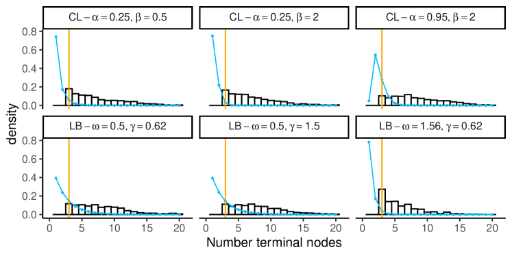
Figure 7: Number of terminal nodes posterior distributions using different priors for the tree topology. The posteriors are obtained by running 10 parallel chains each one composed of 1000 steps and burn-in of 200. The priors considered are the classic tree prior (CL) with parameter couples $(\alpha,\beta)=\{(0.25,0.5),(0.25,2),(0.95,2)\}$ and, the loss-based prior (LB) with parameters couples $(\omega,\gamma)=\{(0.5,0.62),(0.5,1.5),(1.56,0.62)\}$. The light blue lines represent the prior distributions, while the vertical orange line represents the true number of terminal nodes.

Figure 8: Depth posterior distributions using different priors for the tree topology. The posteriors are obtained by running 10 parallel chains each one composed of 1000 steps and burn-in of 200. The priors considered are the classic tree prior (CL) with parameters couples $(\alpha,\beta)=\{(0.25,0.5),(0.25,2),(0.95,2)\}$ and, the loss-based prior (LB) with parameter couples $(\omega,\gamma)=\{(0.5,0.62),(0.5,1.5),(1.56,0.62)\}$. The ligh-tblue lines represent the prior distributions, while the vertical orange line represents the true number of terminal nodes

6 Real Data application

In this section we compare the Loss-based prior and the CL prior described in Chipman et al. (1998) using the breast cancer data collected by William HI. Wolberg, University of Wisconsin Hospitals, Madison (Wolberg and Mangasarian, 1990), and already analysed by various authors (Breiman, 1996; Chipman et al., 1998; Wu et al., 2007). The dataset can be downloaded from the University of California Irvine repository of machine-learning databases . The variable of interest is a binary variable indicating whether cancer is malignant (1) or benign (0), therefore we need to consider a different likelihood for the observations. This section is divided in two parts: the first introduces the data and the likelihood and the second explores the results.

6.1 Data and Likelihood

The data provides 9 different predictors corresponding to different cellular characteristics listed in Table 2 and 699 observations. There are 16 observations with missing Bare Nuclei value, we discard them and use only 683 observations in the analysis. The predictors are normalised to vary between 0 and 1.

Variable	Range	Encoding	$Cor(X_{i},Y)$
Clump Thickness	1-10	$X_{1}$	0.714
Uniformity of Cell Size	1-10	$X_{2}$	0.820
Uniformity of Cell Shape	1-10	$X_{3}$	0.821
Marginal Adhesion	1-10	$X_{4}$	0.706
Single Epithelial Cell Size	1-10	$X_{5}$	0.690
Bare Nuclei	1-10	$X_{6}$	0.822
Bland Chromatin	1-10	$X_{7}$	0.758
Normal Nucleoli	1-10	$X_{8}$	0.718
Mitoses	1-10	$X_{9}$	0.423

Table 2: Table of available predictors in the breast cancer dataset. First column represents the name of the variable, the second represents the domain of the variable, the third represents how the variable is encoded, the fourth column reports the correlation with $Y$ assuming the value 1 if the cancer is malign and 0 otherwise.

The observations are binary in this case and therefore we need to consider a different marginal likelihood for the observations than the one described in Equation 2. We consider a Bernoulli likelihood with probability given by the value of the tree. More formally, given a set of $n$ observations $\mathbf{Y}\in\{0,1\}^{n}$ (in this case $n=683$), a predictors’ matrix $\mathbf{X}\in[0,1]^{n\times p}$ where each row represents an observations with $p$ predictors (in this case $p=9$), and a tree $T$ with terminal node values $M$, we consider

$$\pi(\mathbf{Y}|\mathbf{X},T,M)=\prod_{i=1}^{n}p_{i}^{Y_{i}}(1-p_{i})^{1-Y_{i}},$$ (33)

where $\bm{x}_{i}$ is the $i$-th row of $\mathbf{X}$, $p_{i}$ is the probability of observing $Y_{i}=1$, and it is given by the value of the terminal node corresponding to predictor value $\bm{x}_{i}$, $p_{i}=g(\bm{x}_{i},T,M)$.

Given the new likelihood and role of the terminal nodes values $M=(\mu_{1},...,\mu_{n_{L}(T)})$, which have to satisfy $\mu_{j}\in[0,1]$, the corresponding conjugate prior for $\mu_{j}$ is a Beta distribution with parameters $\alpha_{\mu},\beta_{\mu}$. The conditional posterior distribution is again a Beta distribution with parameters

$$\mu_{j}|\mathbf{Y},\mathbf{X},T\sim\text{Beta}\left(\alpha_{\mu}+\sum_{i}Y_{ij},\beta_{\mu}+n-\sum_{i}Y_{ij}\right)$$ (34)

where $Y_{ij}$ are the observations associated with the $j$-th terminal node. In this example, we consider $\alpha=1,\beta=1$ which corresponds to the uniform prior on the $[0,1]$ interval.

6.2 Results

In this section, we compare the posterior results obtained using the default classic prior with parameters $\alpha=0.95,\beta=2$ and the default loss-based prior with $\omega=1.56,\gamma=0.62$. The two priors provide prior distributions for the number of terminal nodes and depth with different means and tail probabilities as reported in Table 1 (light blue rows). Therefore, we expect the default loss-based prior to provide a stronger penalty and, consequently, to explore shorter trees during the MCMC routine. For both cases, we run 100 chains with starting tree the trivial tree with only one node, and each chain is of length 500. Posterior results are obtained considering a burn-in of 250 samples per chain, Figure 9 shows the traceplots of the log-likelihood for the posterior samples used in the analysis from which it appears that the chains are arrived at convergence. We also considered the classic prior with parameters $\alpha=0.95,\beta=1,0.5$ which performed well in Chipman et al. (1998) and the loss-based prior with parameters $\omega=0.3,0.42,\gamma=1.5,0.5$ which have the same expected number of terminal nodes as the classic prior; results for this additional cases are shown in Appendix 6 as they do not provide further insights.

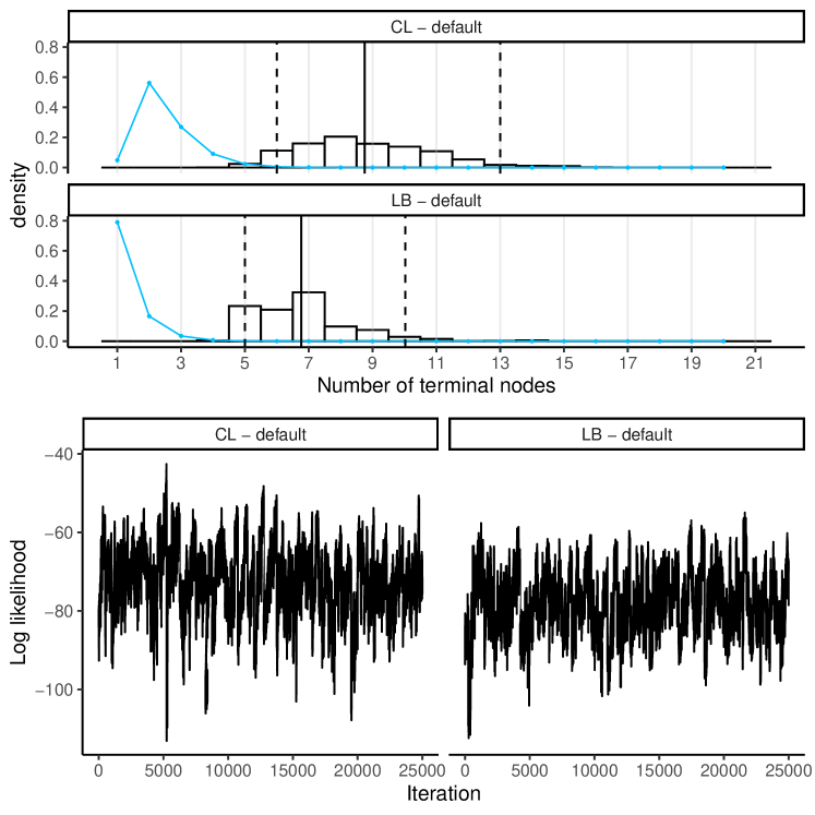
Figure 9: Top panels: Breast cancer data number of terminal nodes posterior distributions using the classic prior with default parameters ($\alpha=0.95,\beta=2$, first top panel) and the loss-based prior with default parameters ($\omega=1.56,\gamma=0.62$, second top panel). Light blue lines represent the prior distributions, black solid vertical lines represent the posterior means while the dashed lines represent $95\%$ posterior credibility intervals. Posterior results are obtained from 100 independent chains each composed of 500 posterior samples and considering a burn-in of 250 samples. Bottom panels: log-likelihood traceplots of the selected posterior samples.

Looking at the posterior distributions of the number of terminal nodes reported in Figure 9 we can see that, as expected, the default loss-based prior provides a posterior distribution more concentrated around low values of the number of terminal nodes. Indeed, the posterior mean of the number of terminal nodes (vertical solid lines) are 8.75 for the CL prior and 6.76 for the loss-based tree prior, while the $95\%$ posterior credibility intervals (vertical dashed lines) are $(6,13)$ for the CL prior and $(5,10)$ for the loss-based prior. We notice that the trees explored by the loss-based prior, despite being shorter, provide the same levels of log-likelihood as those explored by the CL prior. This is confirmed by Figure 10 which shows that using the loss-based prior all the trees visited with more than 12 nodes have high log-likelihood, while when using the CL prior they are more disperse. The same is true if we look at the missing rates versus the number of terminal nodes shown in Figure 11.

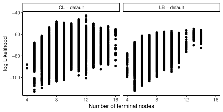
Figure 10: Log likelihood as a function of the number of terminal nodes of the trees explored during the MCMC routine.

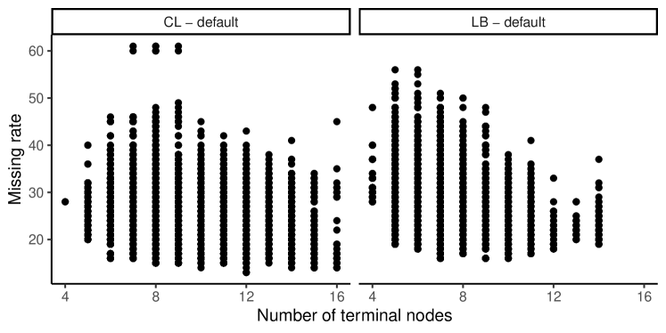
Figure 11: Missing rate as a function of the number of terminal nodes of the trees explored during the MCMC routine.

Figure 12 combines the information in Figures 10 and 11. From this figure is clear that using the loss-based prior the trees with high numbers of terminal nodes are also the ones with the highest log-likelihood and less variable missing rate. In contrast, using the CL prior with default parameters the trees with high number of terminal nodes do not provide a clear advantage in terms of log-likelihood and missing rate than the simpler ones. Looking at the loss-based prior we see that as the number of terminal nodes increases the log-likelihood is more concetrated around high values; this is not as clear for the CL prior. This is an important benefit of using the defualt loss-based prior over the default classic prior for this problem as it provides shorter trees with the same predictive capabilities and log-likelihood than the more complex ones explored under the CL prior. However, the CL prior is capable of achieving the highest log-likelihood (CL$=-42.60$, LB$=-54.97$) and lowest missing rate (CL$=13$, LB$=16$).

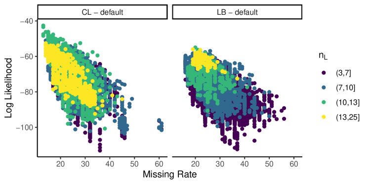
Figure 12: Log likelihood as a function of the missing rate for different number of terminal nodes classes (color) of the trees explored during the MCMC routine.

7 Discussion and conclusions

In this article, we have applied the loss-based prior approach proposed by Villa and Walker (2015b) to design a prior for the tree structure of the BART and CART models. The obtained prior penalises both for the number of terminal nodes and the difference between left and right terminal nodes giving more control over the shape of the trees. A uniform distribution is considered over trees with the same number of terminal nodes and difference between left and right terminal nodes. The prior proposed in this article is objective and can be calibrated objectively by maximising the expected loss. Furthermore, it turns out that following this approach the distribution of the number of terminal nodes is a Geometric distribution. This provides an advantage when we want to incorporate prior information in the model and it is possible to set the parameters in a way that the prior probability that the number of terminal nodes exceeds a certain threshold is below a certain value. Also, the loss-based prior is convenient from a computational point of view because we only need to know the number of terminal nodes ($n_{L}$) and the difference between left and right terminal nodes ($\Delta$) to calculate the prior for a tree. During the MCMC routine, this information can be easily retrieved by knowing the tree at the previous step and the move to be performed at the current step, so that the prior for the new tree can be calculated efficiently. The proposed prior can also be combined with priors on the splitting rules designed for specific goals (e.g. variable selection) such as the one proposed by Rocková and van der Pas (2017) and Linero (2018). This would provide an even stronger penalty on complex trees that can be useful in some applied problems where we are interested in keeping the complexity of the tree under control.

We have compared the performance of the proposed loss-based prior and the CL prior proposed by Chipman et al. (1998) using synthetic and real data. What is important in this comparison is the usual tradeoff between complexity of the tree and ability to explain the data (this can be seen in terms of log-likelihood or other measures of goodness-of-fit). Essentially, we would like to visit trees as short as possible but providing a good fit to the data and we want to avoid complex trees that do not provide a clear advantage. We have shown that the default loss-based prior penalises more for complexity than the default CL prior. The effects of having a stronger penalty are clearly visible in the breast cancer data example, where shorter trees are visited using the loss-based prior but with similar values in terms of log-likelihood and missing rate than the more complex ones visited under the CL prior. This is an advantage because it means that with the default loss-based prior we find shorter trees that explain the data as well as the more complex ones visited under the default CL prior. Moreover, we have shown in the synthetic data example, that also when considering loss-based priors calibrated to replicate CL priors, the number of terminal nodes and depth posterior distributions are more concentrated around low values of the variables. This again shows that the loss-based prior applies a stronger penalty for tree complexity even when the prior information is similar.

The loss-based prior approach described and used in this paper is not limited to the tree structure and can potentially be applied to other parts of the model, therefore providing a unified and objective framework to design priors for BART and CART answering different needs. Specifically, regarding the tree structure the prior we introduced in this paper is not the only one that can be obtained. Indeed, the approach is flexible and depends on which tree statistics are used in the defining the loss in complexity. For example, in early experiments we used the depth of the tree and a conditional distribution on the number of terminal nodes given the depth. This prior did not perform well in synthetic experiments and we had to change it. Nevertheless this testifies to the flexibility of the approach and the ability to target specific tree’s statistics and potentially tailor the loss-based prior on the problem at hand. This approach can also be used to design priors for other quantities. For example, it has already been used to perform variable selection (Villa and Lee, 2020) and therefore it could be used to design a prior on the splitting rules that penalises for the number of predictors used in a tree. Along the same lines, it can be used to design a prior distribution on the number of trees in BART. This would be highly beneficial because for now (w.r.t the authors knowledge) we do not do inference on this quantity which is considered as a tuning parameter with default value 200 (Chipman et al., 2010). Having a prior on the number of trees would allow us to make inference on this quantity based on observed data rather than trying different values and subjectively picking the best one. In conclusion, we believe our approach can provide a valuable and fruitful addition to the BART/CART model literature with the potential of opening up new lines of research in this field.

8 Data availability statement

The breast cancer data used in Section 6 has been collected by William HI. Wolberg, University of Wisconsin Hospitals, Madison (see Wolberg and Mangasarian 1990), and already analysed by various authors. The dataset can be downloaded from the University of California Irvine repository of machine-learning databases . The code used to produce the analyses in Section 5 and 6 as well as all the figures of the article is publicly available on GitHub .

Appendix A Appendix A: Kullback-Liebler divergence

In this section, I report the minimum Kullback-Liebler divergence between a CART model with $N$ terminal nodes and one with $N-1$ terminal nodes. I call $T$ the tree with $N$ terminal nodes, inducing the partition $\bm{\Omega}=\{\Omega_{k}\}_{k=1}{N}$ of the predictors space $\mathcal{X}$ and terminal node values $M=\mu_{1},...,\mu_{N}$, and $T^{\prime}$ the tree with $N-1$ terminal nodes, inducing the partition $\bm{\Omega}^{\prime}=\{\Omega^{\prime}_{k}\}_{k=1}^{N-1}$ and terminal nodes value $M^{\prime}=\mu^{\prime}_{1},...,\mu^{\prime}_{N-1}$. The two models induce a distribution of the data given by

$$\pi(y|\bm{x},T,M)=\sum_{k=1}^{N}\mathbb{I}(\bm{x}\in\Omega_{k})\phi(y,\mu_{k},\sigma^{2}),$$ (35)

and

$$\pi(y|\bm{x},T^{\prime},M^{\prime})=\sum_{k=1}^{N-1}\mathbb{I}(\bm{x}\in\Omega^{\prime}_{k})\phi(y,\mu^{\prime}_{k},\sigma^{2}),$$ (36)

where $\bm{x}$ is the predictors vector associated with observation $y$, $\mathbb{I}(\bm{x}\in\Omega_{k})$ is an indicator function assuming value $1$ if the condition is met and 0 otherwise, and $\phi(x,\mu,\sigma^{2})$ is a Gaussian density with mean $\mu$ and variance $\sigma^{2}$. From now on, we ignore the marginal variance $\sigma^{2}$ as it is the same for both models.

The KLD between tree $T$ and $T^{\prime}$ is then given by

$$KL(T||T^{\prime}|\bm{x}) =\int_{\mathbb{R}^{N}}\left(\int_{\mathbb{R}^{N-1}}\left(\int_{\mathcal{Y}}\pi(y|\bm{x},T,M)\log\left(\frac{\pi(y|\bm{x},T,M)}{\pi(y|\bm{x},T^{\prime},M^{\prime})}\right)dy\right)\pi(M^{\prime})dM^{\prime}\right)\pi(M)dM,$$ (37)

$$=\mathbb{E}_{M}\left(\mathbb{E}_{M^{\prime}}\left(\int_{\mathcal{Y}}\pi(y|\bm{x},T,M)\log\left(\frac{\pi(y|\bm{x},T,M)}{\pi(y|\bm{x},T^{\prime},M^{\prime})}\right)dy\right)\right),$$ (38)

$$=\mathbb{E}_{M}\left(\mathbb{E}_{M^{\prime}}\left(\sum_{k=1}^{N}\mathbb{I}(\bm{x}\in\Omega_{k})\int_{\mathcal{Y}}\phi(y,\mu_{k})\log\left(\frac{\phi(y,\mu_{k})}{\sum_{j=1}^{N-1}\mathbb{I}(\bm{x}\in\Omega^{\prime}_{j})\phi(y,\mu^{\prime}_{j})}\right)dy\right)\right)$$ (39)

where $\mathcal{Y}$ is the observations’ domain. We remove the dependance on the values at the terminal nodes by taking the expected value with respect the prior distribution.

Suppose now that $\bm{x}\in\Omega_{k^{*}}$ w.r.t. $T$, and $\bm{x}\in\Omega^{\prime}_{j^{*}}$ w.r.t. $T^{\prime}$, this simplifies the KLD to

$$KL(T||T^{\prime}|\bm{x}) =\mathbb{E}_{\mu_{k^{*}}}\left(\mathbb{E}_{\mu^{\prime}_{j^{*}}}\left(\int_{\mathcal{Y}}\phi(y,\mu_{k^{*}})\log\left(\frac{\phi(y,\mu_{k^{*}})}{\phi(y,\mu^{\prime}_{j^{*}})}\right)dy\right)\right)$$

$$=\mathbb{E}_{\mu_{k^{*}}}\left(\mathbb{E}_{\mu^{\prime}_{j^{*}}}\left(\int_{\mathcal{Y}}\phi(y,\mu_{k^{*}})\log\phi(y,\mu_{k^{*}}))dy-\int_{\mathcal{Y}}\phi(y,\mu_{k^{*}})\log\phi(y,\mu^{\prime}_{j^{*}}))dy\right)\right).$$

Notice that the expectations now are with respect to the prior distribution of $\mu_{k^{*}}$ and $\mu^{\prime}_{j^{*}}$

Considering that

$$\int_{\mathcal{Y}}\phi(y,\mu_{k^{*}})\log\phi(y,\mu_{k^{*}})dy=\log\left(\frac{1}{\sqrt{2\pi\sigma^{2}}}\right)-\frac{1}{2},$$ (40)

and

$$\int_{\mathcal{Y}}\phi(y,\mu_{k^{*}})\log\phi(y,\mu_{j^{*}})dy=\log\left(\frac{1}{\sqrt{2\pi\sigma^{2}}}\right)-\frac{1}{2}-\frac{\mu_{k^{*}}^{2}}{2\sigma^{2}}+\frac{\mu_{k^{*}}\mu^{\prime}_{j^{*}}}{\sigma^{2}}-\frac{(\mu^{\prime}_{j^{*}})^{2}}{2\sigma^{2}}$$ (41)

we have that

$$KL(T||T^{\prime}|\bm{x}) =\mathbb{E}_{\mu_{k^{*}}}\left(E_{\mu^{\prime}_{j^{*}}}\left(\frac{\mu_{k^{*}}^{2}}{2\sigma^{2}}-\frac{\mu_{k^{*}}\mu^{\prime}_{j^{*}}}{\sigma^{2}}+\frac{{\mu^{\prime}_{j^{*}}}^{2}}{2\sigma^{2}}\right)\right)$$ (42)

$$=\frac{1}{2\sigma^{2}}\mathbb{E}_{\mu_{k^{*}}}\left(E_{\mu^{\prime}_{j^{*}}}\left((\mu_{k^{*}}-\mu^{\prime}_{j^{*}})^{2}\right)\right)$$ (43)

Assuming that $\mu_{k^{*}}$ and $\mu^{\prime}_{j^{*}}$ have the same prior distribution the KLD is zero.

Appendix B Appendix B: Number of binary trees with given number of terminal nodes and left and right terminal nodes difference

In this section, we give the analytical expression of the number of possible binaries trees with fixed number of terminal nodes $n_{L}$, and left and right terminal nodes difference $\Delta$. We start by recalling that the number of possible binary trees with $n$ terminal nodes (with no constrain on $\Delta$) is given by the $n-1$ Catalan number which is

$$C(n)=\frac{(2(n-1))!}{n!(n-1)!}$$ (44)

To determine the possible number of binary trees with fixed $n_{L}$ and $\Delta$. We notice that the couple $n_{L}$, $\Delta$ determines the number of terminal nodes on the right and the left $n_{r}$ and $n_{l}$ through the following system of equations

$$\begin{cases}n_{l}+n_{r}=n_{L}\\ n_{l}-n_{r}=\Delta\end{cases}\quad\text{and}\quad\begin{cases}n_{l}+n_{r}=n_{L}\\ n_{l}-n_{r}=-\Delta\end{cases}$$ (45)

which has solution

$$\begin{cases}n_{l}=\frac{n_{L}+\Delta}{2}\\ n_{r}=\frac{n_{L}-\Delta}{2}\end{cases}\quad\text{and}\quad\begin{cases}n_{l}=\frac{n_{L}-\Delta}{2}\\ n_{r}=\frac{n_{L}+\Delta}{2}\end{cases}$$ (46)

I notice that given that $\Delta$ is odd (even) whenever $n_{L}$ is odd (even) the quantities $n_{L}-\Delta$ and $n_{L}+\Delta$ are always even and, therefore, the solution of the system is always an integer.

Given the above, the total number of possible binary trees with fixed $n_{L}$ and $\Delta$ is equal to the number of possible trees with $n_{l}$ and $n_{r}$ terminal nodes on the left and right branch. More formally, considering there are no contraints on the depth, we have that

$$\mathcal{N}(n_{L},\Delta\neq 0) =C\left(\frac{n_{L}-\Delta}{2}\right)C\left(\frac{n_{L}+\Delta}{2}\right)+C\left(\frac{n_{L}+\Delta}{2}\right)C\left(\frac{n_{L}-\Delta}{2}\right)$$

$$=2C\left(\frac{n_{L}-\Delta}{2}\right)C\left(\frac{n_{L}+\Delta}{2}\right)$$ (47)

where $C(n)$ is the $n-1$ Catalan number counting the number of possible trees with $n$ terminal nodes. This expression is valid only if $\Delta\neq 0$ in which case we have two solutions. When $Delta=0$ the two solutions concides ($n_{l}=n_{r}=n_{L}/2$) and we have

$$\mathcal{N}(n_{L},\Delta=0)=C\left(\frac{n_{L}}{2}\right)^{2}$$ (48)

Replacing Equation 44 into Equations 47 and 48 we can write

$$\mathcal{N}(n,\Delta_{n})=\begin{cases}2\left(\frac{(2(\frac{n-\Delta_{n}}{2}-1))!}{\frac{n-\Delta_{n}}{2}!(\frac{n-\Delta_{n}}{2}-1)!}\right)\left(\frac{(2(\frac{n+\Delta_{n}}{2}-1))!}{\frac{n+\Delta_{n}}{2}!(\frac{n+\Delta_{n}}{2}-1)!}\right)&\Delta\neq 0\\ \\ \left(\frac{(2(\frac{n_{L}}{2}-1))!}{\frac{n_{L}}{2}!(\frac{n_{L}}{2}-1)!}\right)^{2}&\Delta=0\end{cases}$$ (49)

Appendix C Connection with Geometric distribution

The prior on the number of terminal nodes $\pi(n_{L})$ used for the loss-based prior formulation is a case of geometric distribution. The geometric distribution for $k=1,...,\infty$ has one parameter $p\in(0,1)$ and probability mass function (PMF) defined by

$$\Pr(X=k)=(1-p)^{k-1}p,\quad k=1,...$$ (50)

the prior on the number of terminal node $\pi(n_{L})$ has one parameter $\omega>0$ and PMF given by

$$\Pr(n=k)=e^{-\omega k}(e^{\omega}-1),\quad k=1,...$$ (51)

The two expressions are the same considering $p=1-e^{-\omega}$, in fact

$$\Pr(X=k) =e^{-\omega(k-1)}(1-e^{-\omega})$$

$$=e^{-\omega k}e^{\omega}(1-e^{-\omega})$$

$$=e^{-\omega k}(e^{\omega}-1)$$

Appendix D Trace plots for the simulation experiment

Below are reported the trace plots of the number of terminal nodes, the depth and the likelihood regarding the simulation experiment described in Section 5.

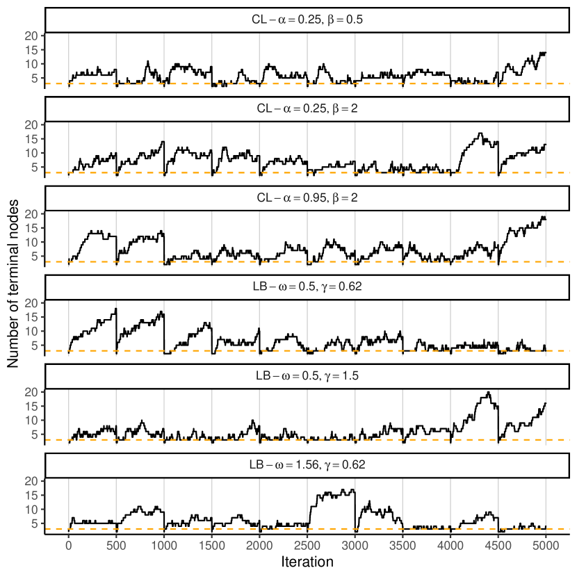
Figure 13: Number of terminal nodes trace plots considering different priors for the tree topology. The plots are obtained by running 10 parallel chains each one composed by 1000 steps. The priors considered are the classic tree prior (CL) with parameters couples $(\alpha,\beta)=\{(0.25,0.5),(0.25,2),(0.95,2)\}$ and, the loss-based prior (LB) with parameters couples $(\omega,\gamma)=\{(0.5,0.62),(0.5,1.5),(1.56,0.62)\}$. The horizontal orange line represents the number of terminal nodes of the data-generating tree.

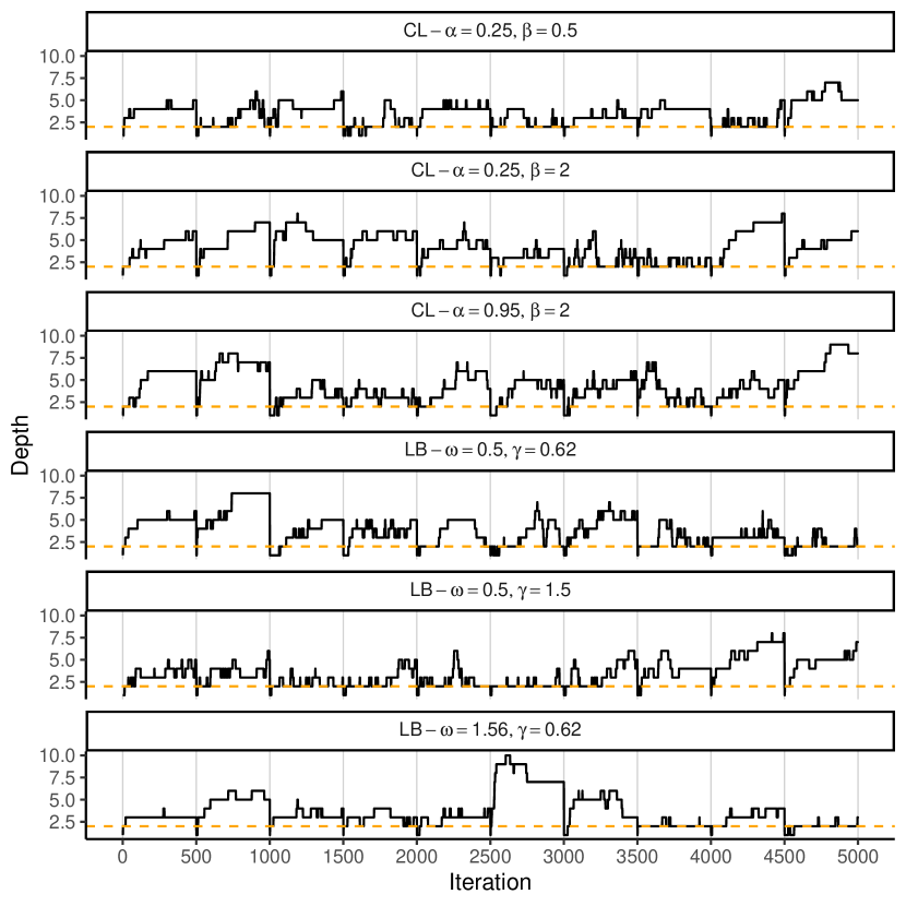
Figure 14: Depth trace plots considering different priors for the tree topology. The plots are obtained by running 10 parallel chains each one composed by 1000 steps. The priors considered are the classic tree prior (CL) with parameters couples $(\alpha,\beta)=\{(0.25,0.5),(0.25,2),(0.95,2)\}$ and, the loss-based prior (LB) with parameters couples $(\omega,\gamma)=\{(0.5,0.62),(0.5,1.5),(1.56,0.62)\}$. The horizontal orange line represents the depth of the data-generating tree.

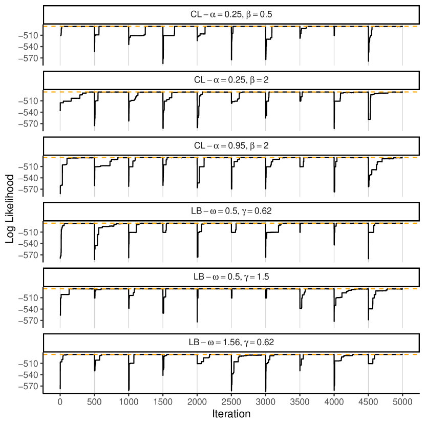
Figure 15: Log-likelihood trace plots considering different priors for the tree topology. The plots are obtained by running 10 parallel chains each one composed by 1000 steps. The priors considered are the classic tree prior (CL) with parameters couples $(\alpha,\beta)=\{(0.25,0.5),(0.25,2),(0.95,2)\}$ and, the loss-based prior (LB) with parameters couples $(\omega,\gamma)=\{(0.5,0.62),(0.5,1.5),(1.56,0.62)\}$. The horizontal orange line represents the log-likelihood using the data-generating tree.

Appendix E Breast cancer data - Additional models results

In this Section, we report the results on the breast cancer data of 6 additional models. We have considered the 2 classic tree priors with parameters $\alpha=0.95,\beta=1,1.5$ which were also considered in (Chipman et al., 1998). For each of these, we find the value of $\omega$ of the loss-based prior providing the same expected number of terminal nodes, we find out that $\omega=0.3$ replicates $\alpha=0.95,\beta=1$ while $\omega=0.42$ replicates $\alpha=0.95,\beta=1.5$. For both values of $\omega$ we consider two values of $\gamma=0.5,1.5$, for a total of 6 models. Figure 16 shows that we find very similar posterior distributions of the number of terminal nodes.

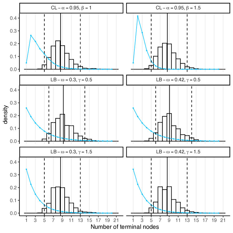
Figure 16: Breast cancer data number of terminal nodes posterior distribution for different priors and parameters (reported in the panel title). Light blue lines represents the prior distributions, the solid vertical lines represent the posterior mean, while dashed vertical lines represent the posterior $95\%$ credibility interval.

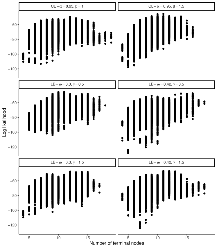
Figure 17: Breast cancer log likelihood as a function of the number of terminal nodes of the trees explored during the MCMC routine for different priors and parameters (reported in the panel title)

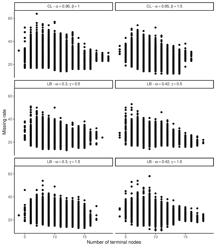
Figure 18: Breast cancer missing rate as a function of the number of terminal nodes of the trees explored during the MCMC routine for different priors and parameters (reported in the panel title)

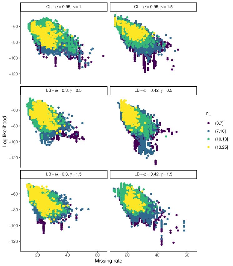
Figure 19: Breast cancer log likelihood as a function of the missing rate for different number of terminal nodes classes (color) of the trees explored during the MCMC routine for different priors and parameters (reported in the panel title).

References

- Berk (1966) Robert H Berk. Limiting behavior of posterior distributions when the model is incorrect. The Annals of Mathematical Statistics, 37(1):51–58, 1966.
- Bonato et al. (2011) Vinicius Bonato, Veerabhadran Baladandayuthapani, Bradley M Broom, Erik P Sulman, Kenneth D Aldape, and Kim-Anh Do. Bayesian ensemble methods for survival prediction in gene expression data. Bioinformatics, 27(3):359–367, 2011.
- Breiman (1996) Leo Breiman. Bagging predictors. Machine learning, 24:123–140, 1996.
- Breiman (2017) Leo Breiman. Classification and regression trees. Routledge, 2017.
- Chipman et al. (2006) Hugh Chipman, Edward George, and Robert McCulloch. Bayesian ensemble learning. Advances in neural information processing systems, 19, 2006.
- Chipman et al. (1998) Hugh A Chipman, Edward I George, and Robert E McCulloch. Bayesian cart model search. Journal of the American Statistical Association, 93(443):935–948, 1998.
- Chipman et al. (2010) Hugh A. Chipman, Edward I. George, and Robert E. McCulloch. BART: Bayesian additive regression trees. The Annals of Applied Statistics, 4(1):266 – 298, 2010. doi: 10.1214/09-AOAS285. URL https://doi.org/10.1214/09-AOAS285.
- Chipman et al. (2022) Hugh A Chipman, Edward I George, Robert E McCulloch, and Thomas S Shively. mbart: multidimensional monotone bart. Bayesian Analysis, 17(2):515–544, 2022.
- Denison et al. (1998) David GT Denison, Bani K Mallick, and Adrian FM Smith. A bayesian cart algorithm. Biometrika, 85(2):363–377, 1998.
- Dorie et al. (2024) Vincent Dorie, Hugh Chipman, and Robert McCulloch. dbarts: Discrete Bayesian Additive Regression Trees Sampler, 2024. URL https://CRAN.R-project.org/package=dbarts. R package version 0.9-26.
- Grazian et al. (2020) Clara Grazian, Cristiano Villa, and Brunero Liseo. On a loss-based prior for the number of components in mixture models. Statistics & Probability Letters, 158:108656, 2020.
- Hahn et al. (2020) P Richard Hahn, Jared S Murray, and Carlos M Carvalho. Bayesian regression tree models for causal inference: Regularization, confounding, and heterogeneous effects (with discussion). Bayesian Analysis, 15(3):965–1056, 2020.
- Hastie and Tibshirani (2000) Trevor Hastie and Robert Tibshirani. Bayesian backfitting (with comments and a rejoinder by the authors. Statistical Science, 15(3):196–223, 2000.
- Hill et al. (2020) Jennifer Hill, Antonio Linero, and Jared Murray. Bayesian additive regression trees: A review and look forward. Annual Review of Statistics and Its Application, 7:251–278, 2020.
- Hill (2011) Jennifer L Hill. Bayesian nonparametric modeling for causal inference. Journal of Computational and Graphical Statistics, 20(1):217–240, 2011.
- Hinoveanu et al. (2019) Laurentiu C Hinoveanu, Fabrizio Leisen, and Cristiano Villa. Bayesian loss-based approach to change point analysis. Computational statistics & data analysis, 129:61–78, 2019.
- Hinoveanu et al. (2020) Laurenţiu Cătălin Hinoveanu, Fabrizio Leisen, and Cristiano Villa. A loss-based prior for gaussian graphical models. Australian & New Zealand Journal of Statistics, 62(4):444–466, 2020.
- Jeong and Rockova (2023) Seonghyun Jeong and Veronika Rockova. The art of bart: Minimax optimality over nonhomogeneous smoothness in high dimension. Journal of Machine Learning Research, 24(337):1–65, 2023.
- Kullback and Leibler (1951) Solomon Kullback and Richard A Leibler. On information and sufficiency. The annals of mathematical statistics, 22(1):79–86, 1951.
- Lamprinakou et al. (2023) Stamatina Lamprinakou, Mauricio Barahona, Seth Flaxman, Sarah Filippi, Axel Gandy, and Emma J McCoy. Bart-based inference for poisson processes. Computational Statistics & Data Analysis, 180:107658, 2023.
- Leisen et al. (2017) Fabrizio Leisen, J Miguel Marin, and Cristiano Villa. Objective bayesian modelling of insurance risks with the skewed student-t distribution. Applied Stochastic Models in Business and Industry, 33(2):136–151, 2017.
- Leisen et al. (2020) Fabrizio Leisen, Luca Rossini, and Cristiano Villa. Loss-based approach to two-piece location-scale distributions with applications to dependent data. Statistical Methods & Applications, 29(2):309–333, 2020.
- Linero (2018) Antonio R Linero. Bayesian regression trees for high-dimensional prediction and variable selection. Journal of the American Statistical Association, 113(522):626–636, 2018.
- Linero et al. (2020) Antonio R Linero, Debajyoti Sinha, and Stuart R Lipsitz. Semiparametric mixed-scale models using shared bayesian forests. Biometrics, 76(1):131–144, 2020.
- Murray (2017) Jared S Murray. Log-linear bayesian additive regression trees for categorical and count responses. arXiv preprint arXiv:1701.01503, 3, 2017.
- Pratola (2016) Matthew T. Pratola. Efficient Metropolis–Hastings Proposal Mechanisms for Bayesian Regression Tree Models. Bayesian Analysis, 11(3):885 – 911, 2016. doi: 10.1214/16-BA999. URL https://doi.org/10.1214/16-BA999.
- Pratola et al. (2020) Matthew T Pratola, Hugh A Chipman, Edward I George, and Robert E McCulloch. Heteroscedastic bart via multiplicative regression trees. Journal of Computational and Graphical Statistics, 29(2):405–417, 2020.
- Rocková (2019) Veronika Rocková. On semi-parametric bernstein-von mises theorems for bart. arXiv preprint arXiv:1905.03735, 2019.
- Ročková and Saha (2019) Veronika Ročková and Enakshi Saha. On theory for bart. In The 22nd international conference on artificial intelligence and statistics, pages 2839–2848. PMLR, 2019.
- Rocková and van der Pas (2017) Veronika Rocková and Stéphanie van der Pas. Posterior concentration for bayesian regression trees and forests. arXiv preprint arXiv:1708.08734, 2017.
- Sparapani et al. (2020) Rodney Sparapani, Brent R Logan, Robert E McCulloch, and Purushottam W Laud. Nonparametric competing risks analysis using bayesian additive regression trees. Statistical methods in medical research, 29(1):57–77, 2020.
- Sparapani et al. (2016) Rodney A Sparapani, Brent R Logan, Robert E McCulloch, and Purushottam W Laud. Nonparametric survival analysis using bayesian additive regression trees (bart). Statistics in medicine, 35(16):2741–2753, 2016.
- Villa and Lee (2020) Cristiano Villa and Jeong Eun Lee. A Loss-Based Prior for Variable Selection in Linear Regression Methods. Bayesian Analysis, 15(2):533 – 558, 2020. doi: 10.1214/19-BA1162. URL https://doi.org/10.1214/19-BA1162.
- Villa and Rubio (2018) Cristiano Villa and Francisco J Rubio. Objective priors for the number of degrees of freedom of a multivariate t distribution and the t-copula. Computational Statistics & Data Analysis, 124:197–219, 2018.
- Villa and Walker (2015a) Cristiano Villa and SG Walker. An objective approach to prior mass functions for discrete parameter spaces. Journal of the American Statistical Association, 110(511):1072–1082, 2015a.
- Villa and Walker (2015b) Cristiano Villa and Stephen Walker. An objective bayesian criterion to determine model prior probabilities. Scandinavian Journal of Statistics, 42(4):947–966, 2015b.
- Villa and Walker (2014) Cristiano Villa and Stephen G. Walker. Objective Prior for the Number of Degrees of Freedom of a t Distribution. Bayesian Analysis, 9(1):197 – 220, 2014. doi: 10.1214/13-BA854. URL https://doi.org/10.1214/13-BA854.
- Wolberg and Mangasarian (1990) William H Wolberg and Olvi L Mangasarian. Multisurface method of pattern separation for medical diagnosis applied to breast cytology. Proceedings of the national academy of sciences, 87(23):9193–9196, 1990.
- Wu et al. (2007) Yuhong Wu, Håkon Tjelmeland, and Mike West. Bayesian cart: Prior specification and posterior simulation. Journal of Computational and Graphical Statistics, 16(1):44–66, 2007.
- Zhang et al. (2020) Tianyu Zhang, Guannan Geng, Yang Liu, and Howard H Chang. Application of bayesian additive regression trees for estimating daily concentrations of pm2. 5 components. Atmosphere, 11(11):1233, 2020.