Data-Driven Room Acoustic Modeling Via Differentiable Feedback Delay Networks With Learnable Delay Lines^†

Abstract

Over the past few decades, extensive research has been devoted to the design of artificial reverberation algorithms aimed at emulating the room acoustics of physical environments. Despite significant advancements, automatic parameter tuning of delay-network models remains an open challenge. We introduce a novel method for finding the parameters of a Feedback Delay Network (FDN) such that its output renders the perceptual qualities of a measured room impulse response. The proposed approach involves the implementation of a differentiable FDN with trainable delay lines, which, for the first time, allows us to simultaneously learn each and every delay-network parameter via backpropagation. The iterative optimization process seeks to minimize a time-domain loss function incorporating differentiable terms accounting for energy decay and echo density. Through experimental validation, we show that the proposed method yields time-invariant frequency-independent FDNs capable of closely matching the desired acoustical characteristics, and outperforms existing methods based on genetic algorithms and analytical filter design.

1 Introduction

Room acoustic synthesis involves simulating the acoustic response of an environment, a task that finds application in a variety of fields, e.g. in music production, to artistically enhance sound recordings; in architectural acoustics, to improve the acoustics of performance spaces; or in VR/AR/computer games, to enhance listeners’ sense of realism [1], immersion [2], and externalization [3].

Room acoustic models can be broadly classified in physical models, convolution models, and delay-network models [4]. Physical ones can be further divided in wave-based models, which provide high physical accuracy but at the cost of significant computational complexity, and geometrical-based ones, which make the simplifying approximation that sound travels like rays. Convolution models involve a set of stored room impulse responses (RIRs) and are therefore capable of replicating the true response of a real room [4]. Convolution is, however, an operation that despite recent advances [5] still carries a computational load that makes them ill-suited in certain real-time applications.

Delay-network models consist of recursively connected networks of delay lines and have a significantly lower computational cost than convolution. Rather than modeling the physical response of a specific room, delay-network models only aim to replicate certain perceptual aspects of room acoustics. These models have a long history, which can be traced back to the Schroeder reverberator [6]. Since then, a number of designs have been proposed, including feedback delay networks (FDNs) [7, 8, 9], scattering delay networks (SDNs) [10], and waveguide networks (WGNs) [11].

The parameters of delay-network models are typically designed to obtain certain desired acoustical characteristics, e.g., a target reverberation time. An alternative design paradigm is to fit the parameters such that the output is as close as possible to that of a measured RIR, hence combining the accuracy of convolution models with the low computational complexity of delay-network models. Several methods following this alternative design paradigm have been recently proposed for the case of FDNs, for instance using gradient-free methods [12, 13, 14, 15, 16] and gradient-based machine learning techniques [17, 18]. Existing approaches, however, involve a certain degree of human intervention and require heuristic-driven ad-hoc choices for several model parameters.

This paper proposes a new method for automatic FDN parameter fitting. The present work is rooted in a recent framework for the parameter estimation of lumped-element models [19] based on automatic differentiation [20], and its novelty is twofold. First, the cost function combines two objective measures of perceptual features, i.e., the energy decay curve (EDC) and a differentiable version of the normalized echo density profile (EDP) [21]. Second, the delay line lengths are optimized via backpropagation along with every other FDN parameter, thus allowing exploiting the flexibility of delay-network models to the fullest. We thus introduce a simple, robust, and fully automatic method for matching acoustic measurements at scale. The learned parameters can be then seamlessly plugged into off-the-shelf FDN software without further processing or mapping.

The paper is organized as follows. Section 2 introduces the background information on FDNs. Section 3 discusses the prior art on automatic FDN parameter tuning. Section 4 describes the proposed method, and Section 5 presents its evaluation. Section 6 concludes the manuscript.

Figure 1: Block diagram of a SISO FDN with $N=3$.

2 Feedback Delay Networks

The block diagram of a single-input-single-output (SISO) FDN is show in Figure 1 [22]. This system is characterized by

$$\begin{array}[]{rl}y[n]&=\mathbf{c}^{T}\mathbf{s}[n]+du[n]\\ \mathbf{s}[n+\bm{m}]&=\mathbf{A}\;\mathbf{s}[n]+\mathbf{b}u[n],\end{array}$$ (1)

where $u[n]$ is the input signal, $y[n]$ is the output signal, $\mathbf{b}\in\mathbb{R}^{N}$ is a vector of input gains, $\mathbf{c}\in\mathbb{R}^{N}$ is a vector of output gains, $(\cdot)^{T}$ denotes the transpose operation, $\mathbf{A}\in\mathbb{R}^{N\times N}$ is the feedback matrix, $d\in\mathbb{R}$ is the scalar gain associated to the direct path, and $\bm{m}=[m_{1},...,m_{N}]$ is a vector containing the length of the $N$ delay lines expressed in samples. The vector $\mathbf{s}[n]\in\mathbb{R}^{N}$ denotes the output of the delay lines at time index $n$, and we use the following notation $\mathbf{s}[n+\bm{m}]=\left[s_{1}[n+m_{1}],...,s_{N}[n+m_{N}]\right]^{T}$ to indicate $N$ parallel delay operations applied to $\mathbf{s}[n]$ of $m_{1},...,m_{N}$ samples, respectively.

If $\bm{m}=[1,...,1]$, then (1) corresponds to the measurement and state equations of a state-space model. In other words, an FDN corresponds to a generalized version of a state-space model with non-unit delays [22].

The standard approach to designing the FDN parameters involves choosing the feedback matrix, delays, and input/output weights so as to obtain certain desired acoustic characteristics—usually a sufficient echo density and a pre-set reverberation time. The most important parameters are the ones associated to the recursive loop, i.e., $\bm{m}$ and $\mathbf{A}$, since they determine the energy decay behavior of the model, as well as its stability. The delays, $\bm{m}$, are typically chosen as co-prime of each other, so as to reduce the number of overlapping echoes and increase the echo density [23]. The design of the feedback matrix, $\mathbf{A}$, starts from a lossless prototype, usually an orthogonal matrix such as Hadamard or Householder matrix, which have been shown to ensure (critical) stability regardless of the delays, a property defined by Schlecht and Habets as unilosslessness [8]. Losses are then incorporated by multiplying the unilossless matrix by a diagonal matrix of scalars designed to achieve a pre-set reverberation time, $T_{60}$.

While it is possible to design feedback matrices as time varying and/or frequency dependent [24, 7], this paper focuses on the time-invariant and frequency-independent case. With this assumption, the stability of the system can be easily enforced throughout the training, thanks to the model reparameterization strategies discussed later in Section 4.

3 Related Work

As mentioned earlier, automatic tuning of FDN parameters has been previously investigated by means of gradient-free methods, such as Bayesian optimization [12] and genetic algorithms [13, 15, 14, 16], as well as gradient-based machine learning techniques [17, 18].

Some works are concerned with the automatic tuning of off-the-shelf reverberation plug-ins. In [25], Heise and colleagues investigate four gradient-free optimization strategies: simulated evolution [26], the Nelder-Mead simplex method [27], Nelder-Mead with brute-force parallelization, and particle swarm optimization [28]. More recently, [12] applies Bayesian optimization using a Gaussian process as a prior to iteratively acquire the control parameters of an external FDN plug-in that minimize the mean absolute error between the multiresolution mel-spectrogram of the target RIR convolved with a 3-second logarithmic sine sweep and that of the artificial reverberator output. The FDN control parameters include the delay line length, reverberation time, fade-in time, high/low cutoff, high/low Q, high/low gain, and dry-wet ratio.

Conversely, other studies assume white-box access to the delay-network structure and apply genetic algorithms (GA) to optimize a subset of the FDN parameters. In [13], a GA is used to find both the $N^{2}$ coefficients of the feedback matrix $\mathbf{A}$ and $N$ cutoff frequencies of lowpass filters, one for each delay line. The authors of [14] aim at finding a mapping between room and FDN parameters for VR/AR applications. To this end, they synthesize the binaural RIR of a set of virtual shoebox rooms, apply a GA to tune the FDN’s delay lines and scalar feedback gain, and use the resulting training pairs to fit a support vector machine (SVM) regressor. In [15], Coggin and Pirkle apply a GA for the estimation of $\bm{m}$, $\mathbf{b}$, and $\mathbf{c}$. For every individual in a generation, attenuation and output filters are designed using the Yule-Walker method. The authors investigate several fitness functions before favoring the Chebyshev distance between the power envelopes of the target and predicted IR. The optimization is run for late reverberation only: the first 85 ms of the RIR are cut and convolved with the input signal, before being fed to the FDN to model late reverberation. Following [15], Ibnyahya and Reiss [16] recently introduced a multi-stage method combining more advanced analytical filter design methods and GAs to estimate the FDN parameters that would best approximate a target RIR in terms of a MFCC-based fitness function, similarly to the cost function used in [25].

Due to the well-known limitations of genetic algorithms, such as the high risk of finding sub-optimal solutions, overall slow convergence rate, and the challenges of striking a good exploration-exploitation balance [29], gradient-based techniques have been recently proposed.

Inspired by groundbreaking research on differentiable digital signal processing [30], Lee et al. [17] let the gradients of a multiresolution spectral loss flow through a differentiable artificial reverberator so that they may reach a trainable neural network tasked with yielding the reverberator parameters. This way, the authors train a convolutional-recurrent neural network tasked with inferring the input, output, and absorption filters of a FDN from a reference reverberation (RIR or speech). It is worth mentioning, however, that it is not the delay-network parameters those that are optimized via stochastic gradient descent, but rather it is the weights of the neural network serving as black-box parameter estimator. As such, the differentiable FDN is effectively used as a processing block in computing the loss of an end-to-end neural network instead of being the target of the optimization process.

In a different vein, several recent works aim at learning lumped parameters via gradient-based optimization directly within the digital structure of the model, and forgo parameter-yielding neural networks altogether [31, 32, 19]. In this respect, automatic differentiation has been recently proposed for learning $\mathbf{A},\mathbf{b},\mathbf{c}$ of an FDN (without parametrizing them as a neural network) so as to minimize spectral coloration and obtain a flat frequency response [18].

In this work, we adopt the latter approach and use the method detailed in the next section to learn the values of $\mathbf{A}$, $\mathbf{b}$, $\mathbf{c}$, $\bm{m}$, and $d$ such that the resulting FDN is capable of modeling perceptually meaningful characteristics of the acoustic response of real-life environments

4 Proposed Method

The proposed method involves an iterative gradient-based optimization algorithm. As a learning objective, we choose a perceptually-informed loss function, $\mathcal{L}(h,\hat{h})$, between a target RIR, $h[n]$, and the time-domain FDN output, $\hat{h}[n]$, obtained by setting the FDN input to the Kronecker delta, i.e., $u[n]=\delta[n]$.

We initialize the FDN parameters with no prior knowledge of $h[n]$. Then, at the beginning of each iteration, we calculate $\hat{h}[n]$ by evaluating (1) while freezing the current parameter estimates. Thus, we evaluate $\mathcal{L}(h,\hat{h})$. Finally, each trainable FDN parameter $\theta$ undergoes an optimization step using the error-free gradient $\nabla_{\theta}\mathcal{L}$ computed via reverse-mode automatic differentiation [20].

A typical approach is to use a delay network to only model the late reverberation while handling early reflections separately [12, 14, 15, 16]. Instead, we optimize the FDN such that it accounts for both early and late reverberation at the same time, exploiting thus the advantages of synthesizing the entire RIR with an efficient recursive structure.

At training time, we strip out the initial silence due to direct-path propagation, and disregard every sample beyond the $T_{60}$ of the target RIR. In other words, we only consider the first $L_{T_{60}}:=\left\lceil T_{60}\cdot f_{\mathrm{s}}\right\rceil$ samples of $h[n]$ and $\hat{h}[n]$ in computing the loss. The reason behind restricting the temporal scope only to the segment of the RIR associated with the $T_{60}$ is that, beyond this point, the values involved in the ensuing computations become so small that numerical errors might occur when using single-precision floating-point numbers, and the training process would unwantedly focus on the statistics of background/numerical noise. Notice that, at inference time, i.e., once the FDN parameters have been learned, the room acoustics simulation can be run indefinitely at a very low computational cost.

In this work, we optimize the input gains $\mathbf{b}\in\mathbb{R}_{\geq 0}^{N}$, the output gains $\mathbf{c}\in\mathbb{R}_{\geq 0}^{N}$, the direct gain $d\in\mathbb{R}_{\geq 0}$, the feedback matrix $\mathbf{A}\in\mathbb{R}^{N\times N}$, and the delays $\bm{m}\in\mathbb{R}_{\geq 0}^{N}$ expressed in fractional samples.

4.1 Model Reparameterization

Let $\theta$ be a scalar parameter of the FDN such that $\theta\in\mathbb{X}$ where $\mathbb{X}\subseteq\mathbb{R}$. In general, instead of learning $\theta$ directly, we learn an unconstrained proxy $\tilde{\theta}\in\mathbb{R}$ that maps onto $\theta$ through a differentiable (and possibly nonlinear) function $f:\mathbb{R}\rightarrow\mathbb{X}$. Hence, we can use $f(\tilde{\theta})$ in place of $\theta$ in any computation involved in the forward pass of the FDN. In case of vector-valued parameters $\bm{\theta}\in\mathbb{X}^{N}$, we apply $f$ in an element-wise fashion, i.e., $\bm{\theta}:=[f(\tilde{\theta}_{1}),...,f(\tilde{\theta}_{N})]^{T}$.

The reason behind such an explicit reparameterization method is that, while we would like $\bm{\theta}$ to take values in $\mathbb{X}^{N}$ at every iteration, gradient-based optimization may yield parameters that do not respect such a constraint, even when using implicit regularization strategies, e.g., by means of auxiliary loss functions and regularizers.

In our FDN model, we treat every parameter in a different fashion. We discuss gain reparameterization in Section 4.2 and present the feedback matrix reparameterization in Section 4.3. Finally, we outline the implementation of the differentiable delay lines and their reparameterization in Section 4.4.

4.2 Trainable Gains

We would like the input, output, and direct gains of our differentiable FDN to be nonnegative. This way, the gains only affect the amplitude of the signals and do not risk inverting their polarity. Instead, we let $\mathbf{A}$ model phase-reversing reflections. To enforce gain nonnegativity, we employ a differentiable nonlinear function $f_{\geq 0}:\mathbb{R}\rightarrow\mathbb{R}_{\geq 0}$, such as, e.g., the Softplus or exponential function. We then learn, e.g., $\mathbf{\tilde{b}}=[\tilde{b}_{1},...,\tilde{b}_{N}]^{T}$ while using $\mathbf{b}=[f_{\geq 0}(\tilde{b}_{1}),...,f_{\geq 0}(\tilde{b}_{N})]^{T}$ in every computation concerning the FDN. Among other options, we select $f_{\geq 0}(x)=\lvert x\rvert$ [19], where the requirement of $f_{\geq 0}$ being differentiable everywhere was relaxed as it is common for many widely-adopted activation functions, such as ReLU.

4.3 Trainable Feedback Matrix

We focus on lossy FDNs. In prior work [18], frequency-independent homogeneous decay has been modeled by parameterizing $\mathbf{A}$ as the product of a unilossless matrix $\mathbf{U}$ and a diagonal matrix $\bm{\Gamma}(\bm{m})=\operatorname{diag}\left(\gamma_{1},...,\gamma_{N}\right)=\operatorname{diag}\left(\gamma^{m_{1}},...,\gamma^{m_{N}}\right)$ containing a delay-dependent absorption coefficient for each delay line, where $\gamma\in(0,1)$ is a constant gain-per-sample coefficient. The feedback matrix is thus expressed as

$$\mathbf{A}=\mathbf{U}\bm{\Gamma}(\bm{m}).$$ (2)

We let $\mathbf{U}$ be an orthogonal matrix, satisfying the unitary condition for unilosslessness [33]. To ensure this property, $\mathbf{U}$ is further parametrized by means of $\mathbf{\tilde{W}}\in\mathbb{R}^{N\times N}$ that, at each iteration, yields [18]

$$\mathbf{U}=\exp\!\left(\mathbf{W}_{\text{Tr}}-\mathbf{W}_{\text{Tr}}^{T}\right),$$ (3)

where $\mathbf{W}_{\text{Tr}}$ is the upper triangular part of $\mathbf{\tilde{W}}$, and $\exp(\cdot)$ is the matrix exponential. In other words, instead of trying to directly learn a unilossless matrix, we learn an unconstrained real-valued matrix $\mathbf{\tilde{W}}$ that maps onto an orthogonal matrix through the exponential mapping in (3). In particular, $\mathbf{U}$ is ensured to be orthogonal because $\mathbf{W}_{\text{Tr}}-\mathbf{W}_{\text{Tr}}^{T}$ is skew-symmetric [34]. As for the matrix $\bm{\Gamma}(\bm{m})$, we noticed that tying the values of the absorption coefficients $\gamma_{1},...,\gamma_{N}$ to those of the fractional delays $m_{1},...,m_{N}$ led to instability during training since the values in $\bm{m}$ were concurrently acting on the temporal location of the IR taps as well as their amplitude. Conversely, we decouple $\bm{\Gamma}$ from $\bm{m}$, thus learning a possibly inhomogeneous FDN characterized by $\mathbf{A}=\mathbf{U}\bm{\Gamma}$, as opposed to the homogeneous FDNs studied in [18].

In learning the unconstrained absorption matrix $\bm{\tilde{\Gamma}}=\operatorname{diag}\left(\tilde{\bm{\gamma}}\right)=\operatorname{diag}(\tilde{\gamma}_{1},...,\tilde{\gamma}_{N})$, we define $f_{(0,1)}:\mathbb{R}\rightarrow(0,1)$ and optimize $\tilde{\bm{\gamma}}\in\mathbb{R}^{N}$ so that $\bm{\Gamma}=\operatorname{diag}\left(f_{(0,1)}(\tilde{\gamma}_{1}),...,f_{(0,1)}(\tilde{\gamma}_{N})\right)$. In the following, we use the well-known Sigmoid function to force the absorption coefficients to take values in the range of $0$ to $1$, i.e.,

$$f_{(0,1)}(x)=\frac{1}{1+e^{-x}}.$$ (4)

4.4 Trainable Delay Lines

In the digital domain, an integer delay can be efficiently implemented as a reading operation from a buffer that accumulates past samples. Unfortunately, this approach is non-differentiable. Instead, since the Fourier transform is a linear and differentiable operator, we may think to work in the frequency domain to circumvent such a problem. In particular, we evaluate the delays on the unit circle at discrete frequency points $\omega_{k}=2\pi k/K$, for $k=0,...,K-1$.

Each differentiable delay line comprises a $K$-sample buffer. First, we compute the Discrete Fourier Transform (DFT) of the signal $x[n]$ currently stored in the buffer. Then, we apply a (fractional) delay of $m$ samples by multiplying the resulting spectrum for the complex exponential $e^{-j\omega_{k}m}$. Finally, we go back in the time domain by computing the inverse Fourier transform limitedly to the $n$th time sample. We can express this sequence of differentiable operations as

$$x[n-m]=\frac{1}{K}\sum_{k=0}^{K-1}\mathcal{F}\left\{x[n]\right\}e^{j\omega_{k}(n-m)}\,,$$ (5)

where

$$\mathcal{F}\left\{x[n]\right\}\;=\!\sum_{\tau=-\infty}^{\infty}w[\tau]x[\tau]e^{-j\omega_{k}\tau}\,,$$ (6)

and

$$w[\tau]=\left\{\begin{array}[]{rl}1&\quad n-K\leq\tau\leq n\\ 0&\quad\text{elsewhere}\end{array}\right.$$ (7)

is the rectangular window corresponding to the finite dimension of the buffer. In practice, (6) is implemented as the FFT of the $K$-sample buffered signal. As such, all operations involved in (5) are linear and differentiable.

In addition, delays must be nonnegative to realize a casual system. Hence, we use $f_{\geq 0}$ to ensure nonnegativity of the fractional delays, i.e., $m_{i}=f_{\geq 0}(\tilde{m}_{i})$ where $\tilde{m}_{i}\in\mathbb{R}$ is the $i$th trainable delay-line length proxy, for $i=1,...,N$. Notice that such a parameterization, while enforcing nonegativity, imposes no upper bound on $m_{i}$. An alternative parametrization is $m_{i}=K\cdot f_{(0,1)}(\tilde{m}_{i})$, which ensures that $m_{i}\in(0,K)$ at all times. In this work, we favored the former for its lower computational cost.

Finally, it is worth highlighting three main reasons for labeling our FDN model as time-domain, despite the implementation of differentiable delay lines in the frequency domain. First, frequency-domain operations are confined within the delay filterbank. Second, we stress that our FDN yields the output one sample at a time according to (1). Third, we emphasize the difference between our approach and existing methods implementing every FDN operation in the frequency domain [17, 18].

4.5 Loss Function

Our goal is to learn an FDN capable of capturing the perceptual qualities of a target room. Hence, we avoid pointwise regression objectives such as $L^{p}$-losses between IR taps. Instead, we set out to minimize an error function ($\mathcal{L}_{\text{EDC}}$) between the true and predicted EDCs. Additionally, we use a novel regularization loss ($\mathcal{L}_{\text{EDP}}$) aimed at matching the echo distribution of the target RIR by acting on the normalized EDP. Namely, the composite loss function can be written as

$$\mathcal{L}=\mathcal{L}_{\text{EDC}}+\lambda\mathcal{L}_{\text{EDP}},$$ (8)

where $\lambda\in\mathbb{R}_{\geq 0}$. Similarly to [19], the loss is evaluated in the time domain, and, at each iteration, requires a forward pass through the discrete-time model defined by the current parameter estimates. In the following sections, we will analyze each of the terms in (8).

4.5.1 Energy Decay Curve Loss

For a discrete-time RIR of length $L$, the EDC can be computed through Schroeder’s backward integration [35]

$$\varepsilon[n]=\sum_{\tau=n}^{L}h^{2}[\tau].$$ (9)

Since (9) is differentiable, we can train the FDN to minimize a normalized mean squared error (NMSE) loss defined on the EDCs, i.e.,

$$\mathcal{L}_{\text{EDC}}=\frac{\sum_{n}\left(\varepsilon[n]-\hat{\varepsilon}[n]\right)^{2}}{\sum_{n}\varepsilon[n]^{2}},$$ (10)

where $\hat{\varepsilon}[n]=\sum_{\tau=n}^{L}\hat{h}^{2}[\tau]$.

It is worth noting that, whereas the EDC is typically expressed in dB, (10) is evaluated on a linear scale. The idea is that a linear loss emphasizes errors in the early portion of $\varepsilon[n]$, i.e., where discrepancies are more perceptually relevant [36], compared to a logarithmic loss that would put more focus on the reverberation tail.

4.5.2 Differentiable Normalized Echo Density Profile

In [21], Abel and Huang introduced the so-called normalized echo density profile (EDP) as a means to quantify reverberation echo density by analyzing consecutive frames of the reverberation impulse response. The EDP indicates the proportion of impulse response taps that fall above the local standard deviation. The resulting profile is normalized to a scale ranging from nearly zero, indicating a minimal presence of echoes, to around one, denoting a fully dense reverberation with Gaussian statistics [37].

The EDP is defined as [21]

$$\eta[n]=\frac{1}{\operatorname{erfc}(1/\sqrt{2})}\sum_{\tau=n-\nu}^{n+\nu}w[\tau]\mathbf{1}\!\left\{\lvert h[\tau]\rvert>\sigma_{n}\right\},$$ (11)

where $\operatorname{erfc}(\cdot)$ is the complementary error function,

$$\sigma_{n}=\sqrt{\sum_{\tau=n-\nu}^{n+\nu}w[\tau]h^{2}[\tau]},$$ (12)

is the standard deviation of the $n$th frame, $w[n]$ is a window function of length $2\nu+1$ samples (usually $20$ ms) such that $\sum_{\tau}w[\tau]=1$, and $\mathbf{1}\{\cdot\}$ is an indicator function

$$\mathbf{1}\!\left\{\lvert h[\tau]\rvert>\sigma\right\}=\left\{\begin{array}[]{cc}1&\quad\lvert h[\tau]\rvert>\sigma,\\ 0&\quad\lvert h[\tau]\rvert\leq\sigma.\end{array}\right.$$ (13)

Notably, $\mathbf{1}\{\cdot\}$ is non-differentiable. Thus, the EDP cannot be utilized within our automatic differentiation framework.

To overcome this problem, this section introduces a novel differentiable EDP approximation, which we call soft echo density profile.

First, we notice that the indicator function $\mathbf{1}\!\left\{\lvert h[\tau]\rvert>\sigma\right\}$ can be equivalently expressed as a Heaviside step function $\mathcal{H}\left(\lvert h[\tau]\rvert-\sigma\right)$. Then, we let $g(x)$ denote the Sigmoid function. We define the scaled Sigmoid function $g_{\kappa}(x)=g(\kappa x)$, where $\kappa\in\mathbb{R}_{\geq 0}$. Since

$$\lim_{\kappa\rightarrow\infty}g_{\kappa}(x)=\mathcal{H}(x),$$ (14)

we can define the Soft EDP function as

$$\eta_{\kappa}[n]=\frac{1}{\operatorname{erfc}(1/\sqrt{2})}\sum_{\tau=n-\nu}^{n+\nu}w[\tau]g_{\kappa}\!\left(\lvert h[\tau]\rvert-\sigma_{n}\right),$$ (15)

which approximates (11) for $\kappa\gg 1$.

It is worth mentioning that, whilst the EDP approximation improves as $\kappa$ becomes larger, this also has the side effect of increasing the risk of vanishing gradients. In fact, the derivative of the scaled Sigmoid function can be written as

$$g^{\prime}_{\kappa}(x)=g(\kappa x)\left(1-g(\kappa x)\right),$$ (16)

which approaches zero for large or small inputs. Hence, $g^{\prime}_{\kappa}(x)$ takes on near-zero values outside of a neighborhood of $x=0$ whose size is inversely proportional to $\kappa$, which, in turn, may impede the gradient flow for $\kappa\gg 1$.

In practice, we would like to choose a large value of $\kappa$ but not larger than what is needed. Notably, the need for a large scaling factor is not constant throughout the temporal evolution of a RIR. Early taps are typically sparse, and $\left(\lvert h[\tau]\rvert-\sigma_{n}\right)$ tends to fall within the saturating region of $g_{\kappa}(\cdot)$, even for lower values of $\kappa$. Conversely, in later portions of the RIR, $\kappa$ must take on very large values to contrast the fact that the amplitude of $\left(\lvert h[\tau]\rvert-\sigma_{n}\right)$ progressively decreases. For this reason, we introduce a time-varying scaling parameter, $\kappa_{n}=\xi n+\varrho$, where $\xi\in\mathbb{R}_{>0}$ and $\varrho\in\mathbb{R}_{\geq 0}$ are hyperparameters. Progressively increasing the scaling coefficient has the benefit of enhancing the gradient flow for early decay, while improving the EDP approximation for late reverberation. In general, a more principled definition for $\kappa_{n}$ could be devised, e.g., by tying it to the local statistics of the target RIR or its energy decay. In this work, however, we favor a simple and reproducible approach as it proved to work well in practice.

4.5.3 Soft EDP Loss

Despite the existing trade-off between vanishing gradients and goodness of fit, every operation involved in the computation of (15) is differentiable. This allows us to use the following EDP loss as a regularizer during the FDN training

$$\mathcal{L}_{\text{EDP}}=\frac{1}{L_{T_{60}}}\sum_{n}\left(\eta_{\kappa}[n]-\hat{\eta}_{\kappa}[n]\right)^{2},$$ (17)

where $\hat{\eta}_{\kappa}[n]$ is the Soft EDP of the predicted RIR, and $L_{T_{60}}=\left\lceil T_{60}\cdot f_{\mathrm{s}}\right\rceil$.

4.5.4 Model Summary

Figure 2 summarizes the proposed differentiable FDN model, listing all the unconstrained trainable parameters (top), their dimension, the corresponding reparameterization (middle), and illustrating once again how, through (1), the FDN processes time-domain signals, including unit impulses $\delta[n]$ (bottom).

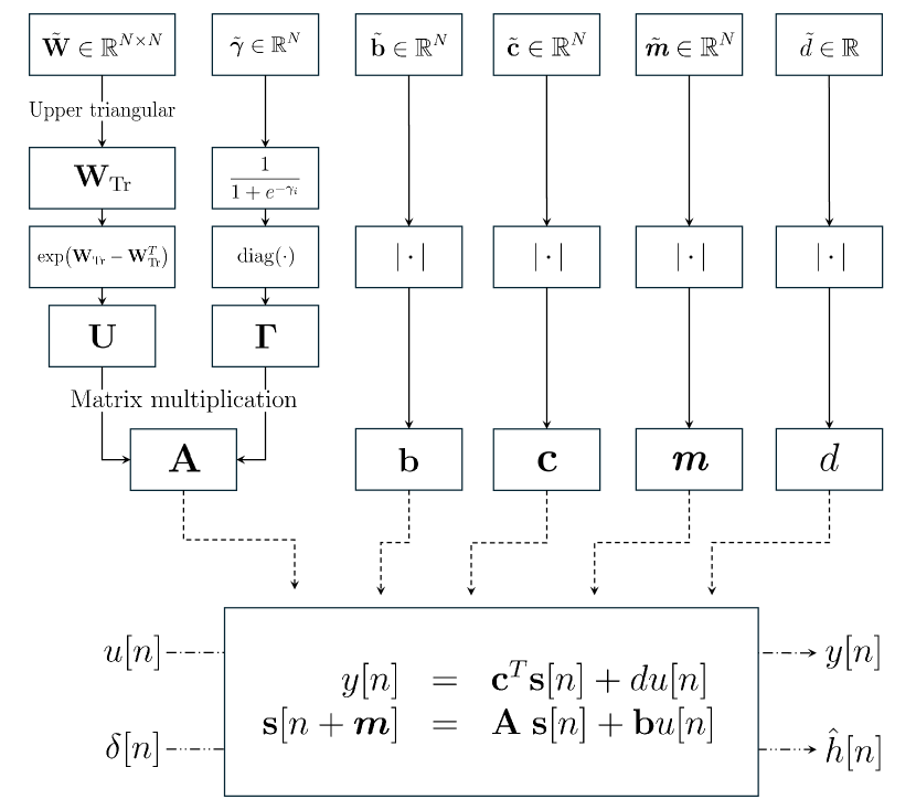
Figure 2: FDN model summary.

5 Evaluation

We evaluate the proposed method using real-world measured RIR from the 2016 MIT Acoustical Reverberation Scene Statistics Survey [38]. The MIT corpus contains single-channel environmental IRs of both open and closed spaces. Of the 271 IRs, we select three according to their reverberation time, which, across the dataset, ranges from a minimum of $0.06$ s to a maximum of $1.99$ s. We select three indoor environments, namely, (i) a small room ($T_{60}\approx 0.2$ s), (ii) a medium room ($T_{60}\approx 0.6$ s), and (iii) a larger room ($T_{60}\approx 1.2$ s). For reproducibility, the ID of the chosen RIRs is reported: (i) h214_Pizzeria_1txts, (ii) h270_Hallway_House_1txts, and (iii) h052_Gym_WeightRoom_3txts. The full IR Survey dataset is available online. For the evaluation, all IRs are resampled to 16 kHz and scaled to unit norm.

5.1 Baseline Method

From the overview presented in Section 3, it appears that no method in the literature is directly comparable with ours. In fact, existing automatic tuning approaches either focus on off-the-shelf reverb plug-ins [25, 12], limit the set of target parameters to just a few [13, 14], or augment the FDN topology with auxiliary frequency-dependent components [15, 16]. To the best of our knowledge, there is no state-of-the-art method addressing the simultaneous estimation of every FDN parameters in a purely data-driven fashion.

Nonetheless, with the aim of comparing our approach with existing techniques, we elect [16] as a baseline by virtue of being arguably the closest to the present work for what concerns the type and number of targeted parameters.

In [16], Ibnyahya and Reiss proposed a multi-stage automatic tuning approach that combines genetic algorithms [39] and analytical filter design [40]. The prototype FDN considered in [16] is equipped with attenuation filters $H_{i}(z)$ and a tone-correction filter $T(z)$ [41]. We depict the model architecture with $N=3$ in Figure 3, featuring the output filter and graphic equalizers for each delay line (cf. Figure 1). Our implementation of [16] uses $N=6$.

The genetic algorithm (GA) is run for five generations, each with a population of 50 FDNs [16]. Each FDN is therefore an individual characterized by $3N+1$ mutable parameters, namely, $\bm{m}$, $\mathbf{b}$, $\mathbf{c}$, and $d$. Throughout the optimization, scalar gains are constrained to take values in $[-1,1]$. Similarly, delays are constrained to take values in the range of 200 µs and 0.25 s [16]. The attenuation filters are analytically determined according to the individual’s delay values in $\bm{m}$ and the desired octave-band reverberation times [40]. In turn, the output graphic EQ filter [42] is found based on the initial level of the desired octave-band EDCs. All individuals implement the same random orthogonal feedback matrix [43], which is not affected by genetic optimization. The fitness of each individual at every generation is assessed through the mean absolute error between the MFCCs of the target RIR and those of the FDN output.

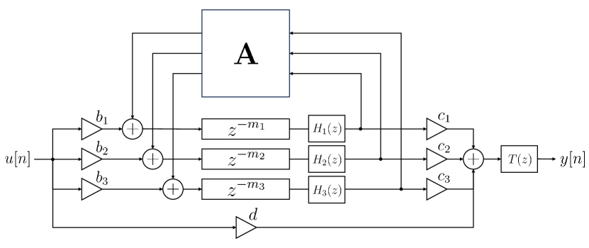
Figure 3: Block diagram of the prototype FDN used in [16].

In our implementation, we avail of the Feedback Delay Network Toolbox (FDNTB) by S. J. Schlecht [44] for fitting the graphic EQ filters and implementing the FDN, and use the GA solver included in MATLAB’s Global Optimization Toolbox for finding $\bm{m}$, $\mathbf{b}$, $\mathbf{c}$, and $d$. From now on, when there is no ambiguity, we will simply refer to this method as our baseline.

It is worth emphasizing the differences between the prototype FDN used in [16] (Figure 3) and the proposed differentiable delay network (Figure 1). First, [16] does not optimize the feedback matrix $\mathbf{A}$, whereas we do. Second, [16] relies on IIR filters to achieve the desired reverberation time, whereas our model does not. Introducing $H_{i}(z)$ and $T(z)$ makes the baseline arguably more powerful in modeling a target RIR. At the same time, though, prior knowledge must be injected into the model by means of filter design to successfully run the GA. In the following, we show that the proposed method is able to model the desired energy decay without augmenting the base FDN architecture described in Section 2.

5.2 Evaluation Metrics

As evaluation metrics, we select the $T_{20}$, $T_{30}$, and $T_{60}$, i.e., the reverberation time extrapolated considering the normalized IR energy decaying from $-5$ dB to $-25$ dB, $-35$ dB, and $-65$ dB, respectively. Ideally, these three metrics are the same if the energy decay exhibits a perfectly linear slope. In practice, this is often not the case, as it can be seen, e.g., in Figure 11. Hence, we believe that it is more informative to report all three of them, as together they provide a richer insight into the global behavior of the EDC as it approaches the $-60$ dB threshold. It is also worth pointing out that it is unclear whether the $T_{60}$ is entirely reliable in measuring the reverberation time of real-world RIRs due to the often non-negligible noise floor.

Moreover, we report clarity ($C_{80}$) in dB [45]

$$C_{80}=10\log_{10}\frac{\sum_{n=0}^{L_{80}-1}h^{2}[n]}{\sum_{n=L_{80}}^{L-1}h^{2}[n]},$$ (18)

where $L_{\tau}=\left\lceil\tau\cdot f_{\mathrm{s}}\cdot 10^{-3}\right\rceil$, definition ($D_{50}$) as a percentage [45]

$$D_{50}=100\cdot\frac{\sum_{n=0}^{L_{50}-1}h^{2}[n]}{\sum_{n=0}^{L-1}h^{2}[n]},$$ (19)

and center time ($t_{s}$) in ms [45]

$$t_{s}=10^{3}\cdot\frac{\sum_{n=0}^{L-1}n\cdot h^{2}[n]}{f_{\mathrm{s}}\cdot\sum_{n=0}^{L-1}h^{2}[n]}.$$ (20)

For all metrics considered, we report the error with respect to the target values. Absolute deviations are denoted by $\Delta$ in Tables 4, 4, and 4.

Finally, it is worth pointing out that the EDPs shown in the following sections are obtained using the (non-differentiable) formulation given in (11), unless explicitly stated otherwise.

5.3 Parameter Initialization

We initialize the differentiable FDN parameters as follows. We let $\mathbf{\tilde{b}}^{(0)}\sim\mathcal{N}(\bm{0},\frac{1}{N}\mathbf{I}_{N})$, where $\mathbf{I}_{N}$ is the $N\times N$ identity matrix. We let $\mathbf{\tilde{c}}^{(0)}=\frac{1}{N}\bm{1}_{N}$, where $\bm{1}_{N}$ is a vector of $N$ ones. As such, the dot product $\mathbf{c}^{T}\mathbf{s}[n]$ in (1) is initially equivalent to the arithmetic average of the outputs of the $N$ delay lines. We set $\tilde{d}^{(0)}=1$. We initialize $\mathbf{\tilde{W}}^{(0)}$ and $\bm{\tilde{\Gamma}}^{(0)}$ so that $\mathbf{\tilde{W}}^{(0)}_{ij}\sim\mathcal{N}(0,\frac{1}{N})$ and $\tilde{\gamma}^{(0)}_{i}\sim\mathcal{N}(0,\frac{1}{N})$. We initialize $\bm{m}^{(0)}$ so that $m^{(0)}_{i}=\psi\tilde{m_{i}}$ with $\tilde{m}_{i}\sim\text{Beta}(\alpha,\beta)$, for $i=1,...,N$, where $\alpha\geq 1$ and $\beta>\alpha$. We empirically set $\psi=1024$, $\alpha=1.1$, and $\beta=6$ to ensure a maximum possible delay of $64$ ms and a mean value of about $10$ ms. We let the Sigmoid scaling term $\kappa_{n}$ increase linearly from $10^{2}$ to $10^{5}$ as $n=0,...,L_{T_{60}}-1$. Finally, we manually tune the hyperparameter $\lambda$ balancing the two loss terms in (8) independently for each test case (see Table 1).

Table 1: Reverberation time, loss values, iteration indices, and linear combination weights $\lambda$. Iterations denoted with $(0)$ indicate pre-training random initialization.

	$T_{60}$ [s]	$\operatorname{iter.}$	$\mathcal{L}$	$\mathcal{L}_{\text{EDC}}$	$\mathcal{L}_{\text{EDP}}$	$\lambda$
Gym (h052)	$1.225$	$(0)$	$1.2070$	$0.9876$	$0.2194$	$1$
		$279$	$0.0201$	$0.0091$	$0.011$
Hallway (h270)	$0.607$	$(0)$	$1.0205$	$0.9904$	$0.3013$	$0.1$
		$340$	$0.0057$	$0.0052$	$0.0046$
Pizzeria (h214)	$0.206$	$(0)$	$0.9589$	$0.9345$	$0.2443$	$0.1$
		$583$	$0.0781$	$0.0766$	$0.0154$

5.4 Implementation Details

We implement our differentiable model in Python using PyTorch. We define the FDN as a class inheriting from nn.Module. We thus define the unconstrained trainable parameters as instances of nn.Parameter. Our model operates at a sampling rate of 16 kHz. As a result, its memory footprint turns out to be contained, allowing us to train all FDNs considered in the present study on a single NVIDIA Titan V graphics card. We optimize the models for a maximum of 650 iterations using Adam [46] with a learning rate of $0.1$, $\beta_{1}=0.9$, $\beta_{2}=0.999$, and no weight decay. In all cases, we present the model with the lowest composite loss.

5.5 Test Case: Gym (h052)

We start by considering the Gym RIR (h052). The FDN is trained setting $\lambda=1$, i.e., equally weighting $\mathcal{L}_{\text{EDC}}$ and $\mathcal{L}_{\text{EDP}}$. As shown in Table 1, the best model is reached at iteration 279, after the loss has decreased by two orders of magnitude with respect to the initial value obtained with the random initialization described in Section 5.3. Below, we offer a comparison between the target room acoustics (solid black line), the baseline algorithm [16] (dash-dotted blue line), and the proposed differentiable FDN optimized for 279 iterations (dashed orange line).

Figure 5, 5, and 6b show that the proposed method is capable of closely matching the EDC, EDP, and envelope of the target RIR, respectively.

Conversely, the baseline method produces poorer results. In Figure 5, we may notice that the EDC appears to overshoot that of target RIR in the first few ms, and that the energy of the IR rapidly decays afterwards, deviating from the target after just 200 ms. Furthermore, the EDP of the baseline method indicates a scarce echo density in the first 250 ms, and that the output of the FDN becomes identically zero just after approximately 0.9 s. The ensuing EDP pathologies are confirmed by the IR depicted in Figure 6a, where the baseline is shown to yield fewer, more prominent taps compared to the IR of the proposed FDN model shown in Figure 6b.

Notably, however, Figure 6 also suggests that both the proposed and baseline methods estimate a larger $d$ than what would correctly render the direct sound. We attribute this phenomenon to an attempt at compensating the lack of a noise floor that, in real-life measurements, contributes to the total energy of the RIR. We argue that, in FDN models with tunable direct gain, offsetting this bias is naively achieved by increasing $d$.

As far as reverberation metrics are concerned, Table 4 shows that the proposed method has an overall better performance, with a $\Delta T_{30}$ and $\Delta T_{60}$ of 2 ms and 40 ms, respectively. The $T_{20}$ is estimated with an error of 100 ms, i.e., approximately 2.5 times lower than that of the baseline method. Similarly, $\Delta C_{80}$ is halved with respect to the baseline, $\Delta D_{50}$ of the proposed method is below 1% that of the target, and $\Delta t_{s}$ is just 59 µs.

Figure 4: EDC of the Gym RIR after 279 iterations.

Figure 5: EDP of the Gym RIR after 279 iterations.

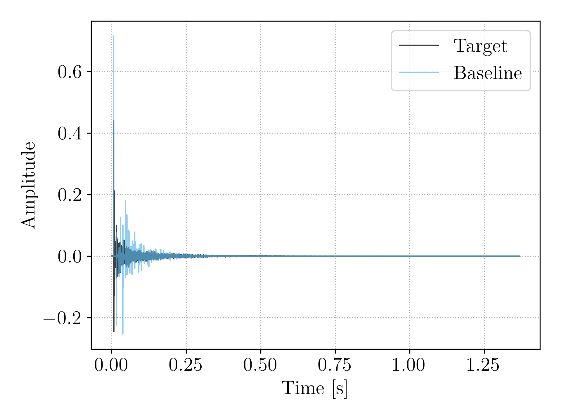
(a)

(b)

Figure 6: IRs of the FDNs approximating the Gym RIR.

Figure 7: EDC of the Hallway RIR after 340 iterations.

Figure 8: EDP of the Hallway RIR after 340 iterations.

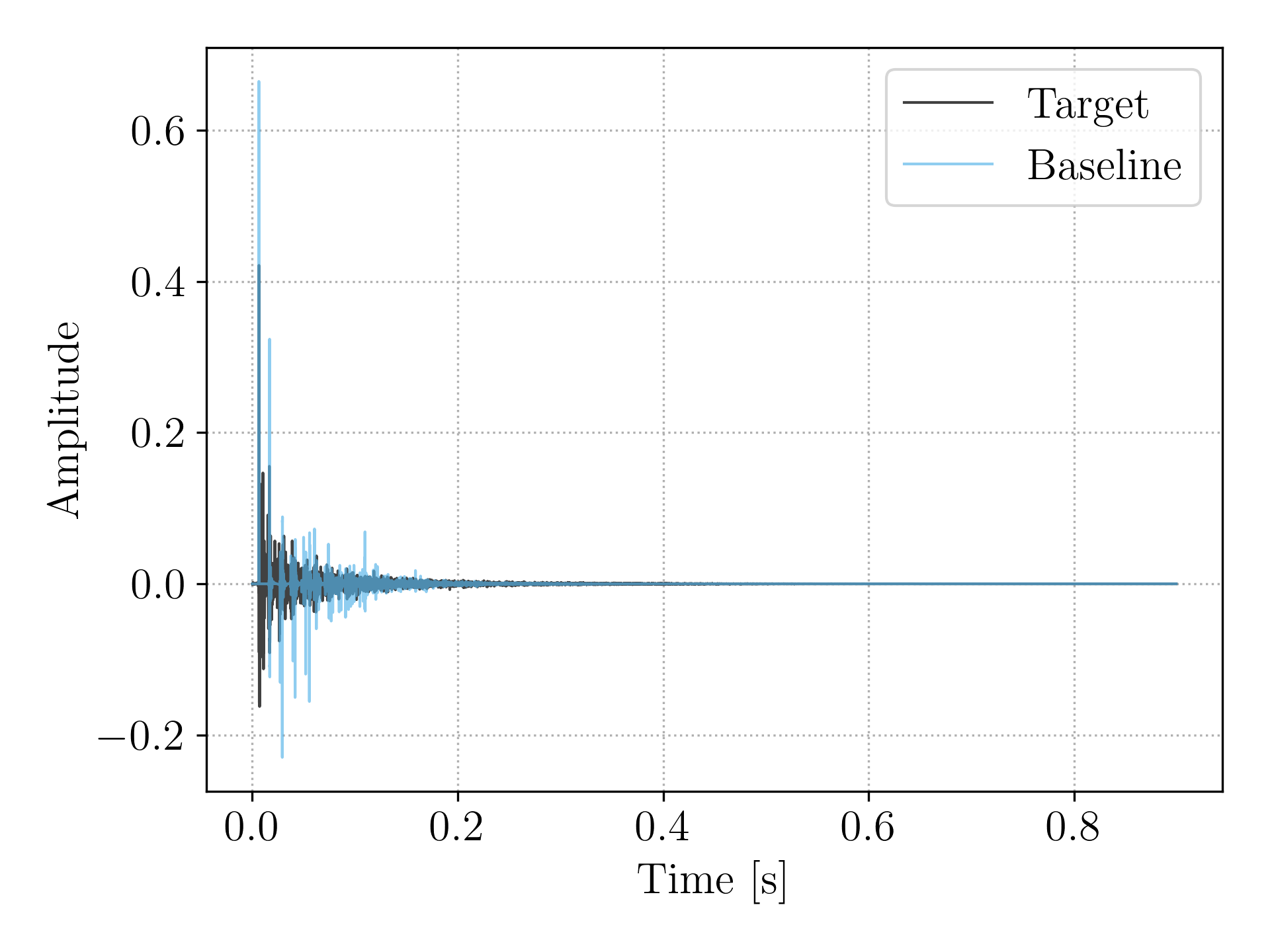
(a)

(b)

Figure 9: IRs of the FDNs approximating the Hallway RIR.

5.6 Test Case: Hallway (h270)

Let us now consider the Hallway RIR (h270), which is characterized by nearly half the $T_{60}$ of the previous case. Table 1 shows that the best results are obtained at iteration 340, where the loss is again lower by two orders of magnitude with respect to the starting point.

Figure 8 reports the EDCs of target (solid black line), baseline (dash-dotted blue line), and predicted (dashed orange line) IRs. Once again, we evince the good matching between our and target decays, as they start to part around $0.4$ s where the residual energy of the predicted RIR is low, i.e., around $-40$ dB. Instead, the baseline is only able to follow the correct decay for less than a third of the total reverberation time, thus providing a result in line with that shown in Section 5.5.

The EDPs depicted in Figure 8 indicate that our approach is able to generate a close match with the target EDP, further validating the effectiveness of proposed Soft EDP loss function. Indeed, the orange dashed curve nicely follows the target curve until the $T_{60}$; we remind, in fact, that the training is performed only on such a span of time. Instead, the EDP of the baseline method shows low values in the first 200 ms compared to the target one, and afterward, even if it takes on comparable values, it does not follow the correct trend. This is confirmed by the RIRs shown in Figure 9. Indeed, even in this test case, the FDN optimized by means of the proposed approach has an IR that resembles more of a realistic RIR, even though the amplitude is not entirely matched.

Table 4 reports the reverberation metrics. We can observe that the proposed optimization approach yields once again better results with respect to the baseline method. Notably, $\Delta T_{30}$ is just 30 ms, while the baseline yields an error of more than 220 ms. The proposed optimization performs better even for all the other metrics. In particular, the error $\Delta C_{80}$ associated with the clarity index is three orders of magnitude less than what can be achieved with the genetic algorithm. In addition, the error $\Delta t_{s}$ on the center time reaches 32 µs, while the baseline has an error of 4.6 ms, which corresponds to shifting the center of mass of the predicted IR energy more toward the reverberation tail.

5.7 Test Case: Pizzeria (h214)

Figure 10: EDC of the Pizzeria RIR after 583 iterations.

Figure 11: EDP of the Pizzeria RIR after 583 iterations.

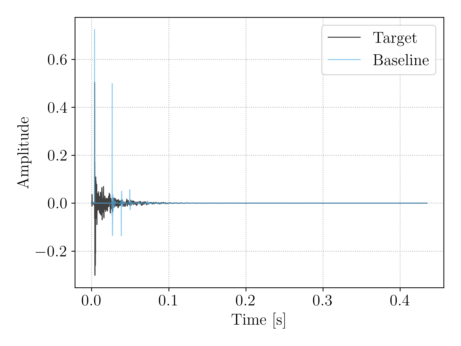
(a)

(b)

Figure 12: IRs of the FDNs approximating the Pizzeria RIR.

Finally, let us address the shortest RIR of the ones considered in the present study, i.e., h214, having a $T_{60}$ of just above 0.2 s.

Here, the baseline method appears to fail at modeling the target room. In particular, the IR shown in Figure 12a exhibits a few sparse taps and it is far from resembling a RIR. Since the backward-integrated energy abruptly decays with every peak, this results in a staircase-like behavior of the EDC depicted in Figure 11.

Facing the same difficulties, the proposed optimization method takes more gradient steps compared to the previous two test cases before finally converging at iteration 583.

In Figure 11, the resulting EDC (dashed orange line) closely follows that of the target RIR (solid black line) until the two reach approximately $-47$ dB. Then, the two deviate before meeting again at $-60$ dB. Still, a direct comparison between EDCs in the range of $-50$ dB to $-70$ dB is not entirely reliable since the RIR has so little energy that background and sensor noise take on a much more relevant role when it comes to integrating the energy of the measured signal.

Overall, the proposed optimization method proves to perform well in fitting the RIR under scrutiny, with Table 4 reporting an error on all three reverberation time metrics of approximately 10 ms, $\Delta D_{50}$ of 0.016%, and $\Delta t_{s}$ of 19 µs.

5.8 Excluding the EDP Loss Term

In developing our method, we noticed that using only the EDC loss function leads to ill-behaved IRs. Namely, we found that, while closely matching the desired EDC, the IR of an FDN trained using only $\mathcal{L}_{\text{EDC}}$, i.e., $\lambda=0$, tends to exhibit an unrealistic echo distribution compared to the RIRs of real-life environments. In this section, we compare the results of our differentiable FDN trained without EDP regularization loss with those presented in Section 5.6 obtained using the composite loss function in (8). For conciseness, we limit our analysis to the Hallway RIR (h270); results obtained with other RIRs are comparable to what is shown below.

When excluding the EDP loss term from (8), the NMSE between true and predicted EDCs (10) is slightly lower than that of the proposed method, i.e., $4.7\times 10^{-3}$ and $5.2\times 10^{-3}$, respectively. Yet, the MSE between true and predicted EDPs (17) is $0.395$, i.e., two orders of magnitude grater than the $0.0046$ reported in Table 1 for the proposed method. This can be observed in Figure 13b, showing that the echo density when $\lambda=0$ (dash-dotted purple line) is far from the desired profile (solid black line). The target RIR and the proposed method (dashed orange line) produce an EDP with values consistently around one, indicating dense reverberation. On the contrary, the FDN trained without Soft EDP regularization yields an EDP with small values, signaling an uneven echo density due to the presence of a few prominent reflections [37]. This observation is confirmed by the IR shown in Figure 13a that exhibits a few clearly noticeable taps peaking above a denser reverberation tail. We argue that this phenomenon occurs when only a few delays are strongly excited, and this turns out to be the case for minimization problems with no constraints discouraging the model to use just a small number of delay lines to capture the overall EDC behavior.

Table 2: Metrics for the Gym RIR ($\lambda=1$).

	$T_{20}$ [s]	$\Delta T_{20}$	$T_{30}$ [s]	$\Delta T_{30}$	$T_{60}$ [s]	$\Delta T_{60}$
Target	$0.8616$	—	$0.9161$	—	$1.2257$	—
Baseline	$0.6202$	$0.2413$	$0.6322$	$0.2839$	$0.7094$	$0.5163$
Ours	$0.7607$	$\mathbf{0.1009}$	$0.9136$	$\mathbf{0.0025}$	$1.1854$	$\mathbf{0.0403}$

	$C_{80}$ [dB]	$\Delta C_{80}$	$D_{50}$ [%]	$\Delta D_{50}$	$t_{s}$ [ms]	$\Delta t_{s}$
Target	$12.1061$	—	$89.0091$	—	$22.8994$	—
Baseline	$11.4695$	$0.6366$	$81.8520$	$7.1571$	$30.0076$	$7.1083$
Ours	$11.8266$	$\mathbf{0.2795}$	$88.2766$	$\mathbf{0.7325}$	$22.9584$	$\mathbf{0.0590}$

Table 3: Metrics for the Hallway RIR ($\lambda=0.1$).

	$T_{20}$ [s]	$\Delta T_{20}$	$T_{30}$ [s]	$\Delta T_{30}$	$T_{60}$ [s]	$\Delta T_{60}$
Target	$0.5289$	—	$0.6010$	—	$0.6067$	—
Baseline	$0.3891$	$0.1399$	$0.3796$	$0.2214$	$0.4102$	$0.1965$
Ours	$0.5031$	$\mathbf{0.0259}$	$0.5716$	$\mathbf{0.0294}$	$0.7023$	$\mathbf{0.0956}$

	$C_{80}$ [dB]	$\Delta C_{80}$	$D_{50}$ [%]	$\Delta D_{50}$	$t_{s}$ [ms]	$\Delta t_{s}$
Target	$14.0797$	—	$90.6917$	—	$20.1163$	—
Baseline	$12.8053$	$1.2743$	$83.9870$	$6.7047$	$24.7643$	$4.6480$
Ours	$14.0713$	$\mathbf{0.0083}$	$90.5123$	$\mathbf{0.1794}$	$20.1487$	$\mathbf{0.0324}$

Table 4: Metrics for the Pizzeria RIR ($\lambda=0.1$).

	$T_{20}$ [s]	$\Delta T_{20}$	$T_{30}$ [s]	$\Delta T_{30}$	$T_{60}$ [s]	$\Delta T_{60}$
Target	$0.1643$	—	$0.1794$	—	$0.2062$	—
Baseline	$0.0703$	$0.0939$	$0.0940$	$0.0854$	$0.1165$	$0.0897$
Ours	$0.1543$	$\mathbf{0.0099}$	$0.1694$	$\mathbf{0.0100}$	$0.2166$	$\mathbf{0.0104}$

	$C_{80}$ [dB]	$\Delta C_{80}$	$D_{50}$ [%]	$\Delta D_{50}$	$t_{s}$ [ms]	$\Delta t_{s}$
Target	$30.9883$	—	$99.3819$	—	$7.1698$	—
Baseline	$37.6095$	$6.6212$	$99.5095$	$0.1275$	$15.7271$	$8.5574$
Ours	$32.1683$	$\mathbf{1.1801}$	$99.3988$	$\mathbf{0.0168}$	$7.1891$	$\mathbf{0.0194}$

5.9 Soft EDP Approximation

Finally, we discuss the approximation capabilities of the proposed Soft EDP function introduced in Section 4.5.2. Figure 14 shows the non-differentiable EDP (solid black line) defined in (11) against several Soft EDP approximations of the three RIRs considered in the present study. We test various scaling parameters $\kappa$, namely $10^{2}$, $10^{3}$, and $10^{4}$, along with the proposed time-varying $\kappa_{n}$ linearly increasing from $10^{2}$ ($n=0$) to $10^{5}$ ($n=L_{T_{60}}-1$). We depict the profiles only for time indices below the $T_{60}$, as this range is the one considered when training the FDNs.

In Figure 14, we may notice that $\kappa=10^{2}$ yields a poor approximation of the reference EDP beyond the very first few ms. We also observe that $\kappa=10^{3}$ and $\kappa=10^{4}$ provide relative improvements. However, after some time, the approximation starts to degrade in a similar fashion as for $\kappa=10^{2}$. Conversely, the proposed Soft EDP with time-varying scaling (dashed orange line) is able to closely match the non-differentiable reference profile all the way up to the $T_{60}$ in Figure 14a, while gracefully combating gradient vanishing (see Section 4.5.2). Notably, however, Figure 14c shows that the approximation in the very last portion of the longest RIR considered, i.e., Gym (h052), significantly differs from the reference profile. To a lesser extent, this is also noticeable in Figure 14b. Nevertheless, it is worth mentioning that, around the estimated $T_{60}$, the energy of the RIR is already almost entirely vanished, and the EDP itself suffers from statistical uncertainty due to sensor and 16-bit quantization noise.

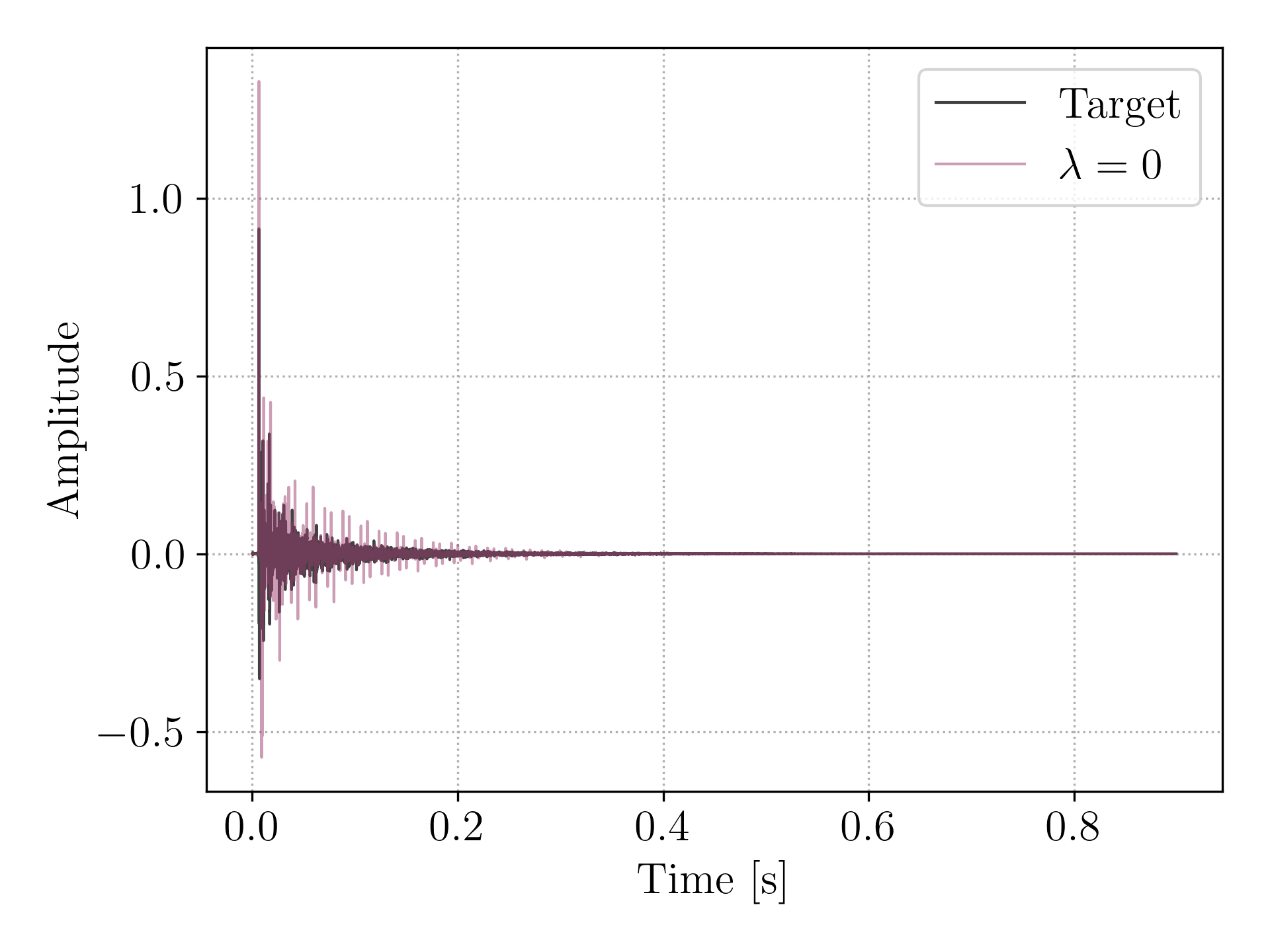
(a)

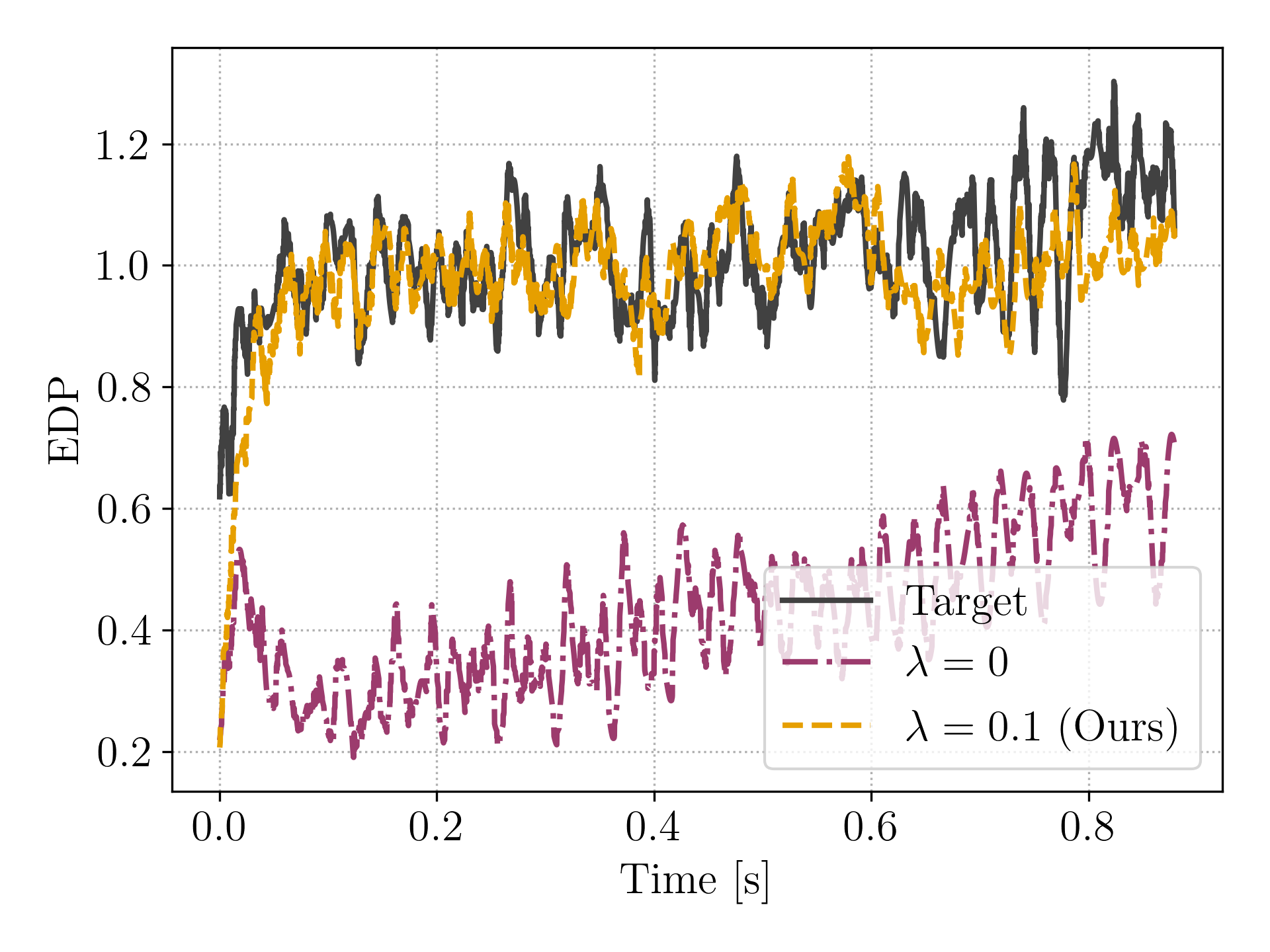
(b)

Figure 13: (a) IR and (b) EDP obtained by training the FDN without EDP regularization loss ($\lambda=0$).

(a)

(b)

(c)

Figure 14: Non-differentiable EDP (Reference) compared with the proposed Soft EDP function for different values of the Sigmoid scaling parameter.

6 Conclusions

We proposed a method for optimizing all the parameters of a time-invariant frequency-independent Feedback Delay Network (FDN) in order to match the reverberation of a given room through perceptually meaningful metrics. In the present work,

• we introduced a fully-differentiable FDN with learnable delay lines,

• we developed a novel optimization framework for all FDN parameters based on automatic differentiation,

• we presented an innovative use of established perceptually-motivated acoustic measures as loss terms,

• we proposed a differentiable implementation of the well-known normalized echo density profile.

In particular, we presented a new differentiable FDN that is characterized by learnable delay lines realized exploiting operations in the frequency domain. We proposed a novel differentiable approximation of the normalized echo density profile, which we call Soft EDP. Thus, we trained the FDN parameters taking into account a composite loss consisting of two terms: the normalized mean square error between target and predicted EDCs and the mean square error between target and predicted Soft EDPs. We tested the methodology on three RIRs of real rooms taken from a publicly available dataset, and we demonstrated that the Soft EDP term is essential for obtaining an IR that resembles a realistic RIR. Finally, we selected as baseline a recent method that tunes a subset of the FDN parameters by means of a genetic algorithm, and we evaluated the methods considering widespread metrics, including reverberation time, clarity, definition, and center time. In all the experiments, the proposed approach was able to consistently outperform the baseline across all the metrics, with errors lower, on average, of one order of magnitude.

Future work includes the application of the proposed approach to frequency-dependent FDNs, which are able to account for a frequency-specific decay in time, or to multiple-input multiple-output (MIMO) delay networks.

Acknowledgments Alessandro Ilic Mezza and Riccardo Giampiccolo wish to thank Xenofon Karakonstantis for the helpful discussion.

Declarations

• Availability of data and materials: The datasets generated and/or analysed during the current study are available on the MIT Acoustical Reverberation Scene Statistics Survey website, https://mcdermottlab.mit.edu/Reverb/IR_Survey.html.

• Funding: This work was partially supported by the European Union under the Italian National Recovery and Resilience Plan (NRRP) of NextGenerationEU, partnership on “Telecommunications of the Future” (PE00000001 — program “RESTART”), and received funding support as part of the JRC STEAM STM–Politecnico di Milano agreement and from the Engineering and Physical Sciences Research Council (EPSRC) under the “SCalable Room Acoustics Modelling (SCReAM)” Grant EP/V002554/1.

• Competing interests: The authors declare that they have no competing interests.

• Authors’ contributions: A. I. Mezza conceptualized the study, designed and implemented the proposed method, run the experiments, and drafted the manuscript. R. Giampiccolo contributed to the design of the proposed method, run the experiments, and drafted part of the manuscript. E. De Sena drafted part of the manuscript. A. Bernardini supervised the work.

References

- \bibcommenthead
- Apostolopoulos et al. [2012] Apostolopoulos, J.G., Chou, P.A., Culbertson, B., Kalker, T., Trott, M.D., Wee, S.: The road to immersive communication. Proc. of the IEEE 100(4), 974–990 (2012)
- Potter et al. [2022] Potter, T., Cvetković, Z., De Sena, E.: On the relative importance of visual and spatial audio rendering on VR immersion. Front. Signal Process. 2 (2022)
- Geronazzo et al. [2020] Geronazzo, M., Tissieres, J.Y., Serafin, S.: A minimal personalization of dynamic binaural synthesis with mixed structural modeling and scattering delay networks. In: Proc. IEEE Int. Conf. Acoust. Speech Signal Process., pp. 411–415 (2020)
- Välimäki et al. [2012] Välimäki, V., Parker, J.D., Savioja, L., Smith, J.O., Abel, J.S.: Fifty years of artificial reverberation. IEEE Trans. Audio Speech Lang. Process. 20(5), 1421–1448 (2012)
- Wefers [2015] Wefers, F.: Partitioned Convolution Algorithms for Real-time Auralization vol. 20. Logos Verlag Berlin GmbH, Berlin, Germany (2015)
- Schroeder [1961] Schroeder, M.R.: Natural sounding artificial reverberation. J. Audio Eng. Soc. 10(3), 219–223 (1961)
- Jot and Chaigne [1991] Jot, J.-M., Chaigne, A.: Digital delay networks for designing artificial reverberators. In: 90th Audio Eng. Soc. Convention (1991)
- Schlecht and Habets [2016] Schlecht, S.J., Habets, E.A.P.: On lossless feedback delay networks. IEEE Trans. Sig. Process. 65(6), 1554–1564 (2016)
- Bai et al. [2015] Bai, H., Richard, G., Daudet, L.: Late reverberation synthesis: From radiance transfer to feedback delay networks. IEEE Trans. Audio Speech Lang. Process. 23(12), 2260–2271 (2015) https://doi.org/10.1109/TASLP.2015.2478116
- De Sena et al. [2015] De Sena, E., Hacıhabiboğlu, H., Cvetković, Z., Smith, J.O.: Efficient synthesis of room acoustics via scattering delay networks. IEEE/ACM Trans. Audio Speech Lang. Process. 23(9), 1478–1492 (2015)
- Stevens et al. [2017] Stevens, F., Murphy, D.T., Savioja, L., Välimäki, V.: Modeling sparsely reflecting outdoor acoustic scenes using the waveguide web. IEEE/ACM Trans. Audio Speech Lang. Process. 25(8), 1566–1578 (2017)
- Bona et al. [2022] Bona, R., Fantini, D., Presti, G., Tiraboschi, M., Engel Alonso-Martinez, J.I., Avanzini, F.: Automatic parameters tuning of late reverberation algorithms for audio augmented reality. In: Proc. 17th Int. Audio Mostly Conf., pp. 36–43 (2022). https://doi.org/10.1145/3561212.3561236
- Chemistruck et al. [2012] Chemistruck, M., Marcolini, K., Pirkle, W.: Generating matrix coefficients for feedback delay networks using genetic algorithm. In: 133rd Audio Eng. Soc. Convention (2012)
- Shen and Duraiswami [2020] Shen, J., Duraiswami, R.: Data-driven feedback delay network construction for real-time virtual room acoustics. In: Proc. 15th Int. Audio Mostly Conf., pp. 46–52 (2020)
- Coggin and Pirkle [2016] Coggin, J., Pirkle, W.: Automatic design of feedback delay network reverb parameters for impulse response matching. In: 141st Audio Eng. Soc. Convention (2016)
- Ibnyahya and Reiss [2022] Ibnyahya, I., Reiss, J.D.: A method for matching room impulse responses with feedback delay networks. In: 153rd Audio Eng. Soc. Convention (2022)
- Lee et al. [2022] Lee, S., Choi, H.-S., Lee, K.: Differentiable artificial reverberation. IEEE/ACM Trans. Audio Speech Lang. Process. 30, 2541–2556 (2022) https://doi.org/10.1109/TASLP.2022.3193298
- Dal Santo et al. [2023] Dal Santo, G., Prawda, K., Schlecht, S., Välimäki, V.: Differentiable feedback delay network for colorless reverberation. In: Proc. 26th Int. Conf. Digital Audio Effects, pp. 244–251 (2023)
- Mezza et al. [2023] Mezza, A.I., Giampiccolo, R., Bernardini, A.: Data-driven parameter estimation of lumped-element models via automatic differentiation. IEEE Access 11, 143601–143615 (2023) https://doi.org/10.1109/ACCESS.2023.3339890
- Baydin et al. [2018] Baydin, A.G., Pearlmutter, B.A., Radul, A.A., Siskind, J.M.: Automatic differentiation in machine learning: a survey. J. Mach. Learning Res. 18, 1–43 (2018)
- Abel and Huang [2006] Abel, J.S., Huang, P.: A simple, robust measure of reverberation echo density. In: 121st Audio Eng. Soc. Convention (2006). Audio Engineering Society
- Rocchesso and Smith [1997] Rocchesso, D., Smith, J.O.: Circulant and elliptic feedback delay networks for artificial reverberation. IEEE Trans. Speech Audio Process. 5(1), 51–63 (1997) https://doi.org/10.1109/89.554269
- Schlecht and Habets [2016] Schlecht, S.J., Habets, E.A.P.: Feedback delay networks: Echo density and mixing time. IEEE/ACM Trans. Audio Speech Lang. Process. 25(2), 374–383 (2016)
- Schlecht and Habets [2015] Schlecht, S.J., Habets, E.A.P.: Time-varying feedback matrices in feedback delay networks and their application in artificial reverberation. J. Acoust. Soc. Am. 138(3), 1389–1398 (2015)
- Heise et al. [2009] Heise, S., Hlatky, M., Loviscach, J.: Automatic adjustment of off-the-shelf reverberation effects. In: 126th Audio Eng. Soc. Convention (2009)
- Fogel [1999] Fogel, L.J.: Intelligence Through Simulated Evolution: Forty Years of Evolutionary Programming. John Wiley & Sons, Inc., Hoboken, NJ, USA (1999)
- Nelder and Mead [1965] Nelder, J.A., Mead, R.: A simplex method for function minimization. Comput. J. 7(4), 308–313 (1965)
- Kennedy and Eberhart [1995] Kennedy, J., Eberhart, R.: Particle swarm optimization. In: Proc. Int. Conf. Neural Netw., vol. 4, pp. 1942–1948 (1995)
- Črepinšek et al. [2013] Črepinšek, M., Liu, S.-H., Mernik, M.: Exploration and exploitation in evolutionary algorithms: A survey. ACM Comput. Surv. 45(3), 1–33 (2013)
- Engel et al. [2020] Engel, J., Hantrakul, L.H., Gu, C., Roberts, A.: DDSP: Differentiable digital signal processing. In: Int. Conf. Learning Representations (2020)
- Esqueda et al. [2021] Esqueda, F., Kuznetsov, B., Parker, J.D.: Differentiable white-box virtual analog modeling. In: Proc. 23rd Int. Conf. Digital Audio Effects, pp. 41–48 (2021)
- Shintani et al. [2022] Shintani, M., Ueda, A., Sato, T.: Accelerating parameter extraction of power mosfet models using automatic differentiation. IEEE Trans. Power Electron. 37(3), 2970–2982 (2022) https://doi.org/10.1109/TPEL.2021.3118057
- Schlecht and Habets [2016] Schlecht, S.J., Habets, E.A.P.: On lossless feedback delay networks. IEEE Trans. Signal Process. 65(6), 1554–1564 (2016)
- Lezcano-Casado and Martınez-Rubio [2019] Lezcano-Casado, M., Martınez-Rubio, D.: Cheap orthogonal constraints in neural networks: A simple parametrization of the orthogonal and unitary group. In: Int. Conf. Mach. Learning, pp. 3794–3803 (2019)
- Schroeder [1965] Schroeder, M.R.: New method of measuring reverberation time. J. Acoust. Soc. Am. 37(6), 1187–1188 (1965)
- Howard and Angus [2013] Howard, D., Angus, J.: Acoustics and Psychoacoustics. Routledge, London, UK (2013)
- Huang and Abel [2007] Huang, P., Abel, J.S.: Aspects of reverberation echo density. In: 123rd Audio Eng. Soc. Convention (2007)
- Traer and McDermott [2016] Traer, J., McDermott, J.H.: Statistics of natural reverberation enable perceptual separation of sound and space. Proc. Natl. Acad. Sci. 113(48), 7856–7865 (2016) https://doi.org/10.1073/pnas.1612524113
- Goldberg [1989] Goldberg, D.E.: Genetic Algorithms in Search, Optimization, and Machine Learning. Addison-Wesley, Boston, MA, USA (1989)
- Schlecht and Habets [2017] Schlecht, S.J., Habets, E.A.P.: Accurate reverberation time control in feedback delay networks. Proc. Int. Conf. Digital Audio Effects, 337–344 (2017)
- Välimäki and Liski [2016] Välimäki, V., Liski, J.: Accurate cascade graphic equalizer. IEEE Signal Process. Lett. 24(2), 176–180 (2016)
- Välimäki and Reiss [2016] Välimäki, V., Reiss, J.D.: All about audio equalization: Solutions and frontiers. Appl. Sci. 6(5) (2016) https://doi.org/10.3390/app6050129
- Edelman and Rao [2005] Edelman, A., Rao, N.R.: Random matrix theory. Acta Numerica 14, 233–297 (2005) https://doi.org/10.1017/S0962492904000236
- Schlecht [2020] Schlecht, S.J.: FDNTB: The feedback delay network toolbox. In: Proc. Int. Conf. Digital Audio Effects, pp. 211–218 (2020)
- [45] Acoustics – Measurement of room acoustic parameters. Part 1: Performance spaces. ISO 3382-1:2009, International Organization for Standardization, Geneva, Switzerland, June 2009
- Kingma and Ba [2015] Kingma, D., Ba, J.: Adam: A method for stochastic optimization. In: Int. Conf. Learning Representations (2015)