Wave-Medium Interactions in Dynamic
Matter and Modulation Systems

Abstract

Space-time modulation systems have garnered significant attention due to their resemblance to moving-matter systems and promising applications. Unlike conventional moving-matter systems, modulation systems do not involve net motion of matter, and are therefore easier to implement and not restricted to subluminal velocities. However, canonical wave-medium interaction aspects, such as scattering and energy-momentum relations, have remained largely unexplored. In this paper, we address the aforementioned issues for three dynamic systems: moving-matter blocs, moving-perturbation interfaces and moving-perturbation periodic structures, and provide corresponding general formulations along with comparisons. Our investigation reveals the significant roles played by the “catch-up” effect between waves and interfaces. Even more interestingly, it reveals different energy and momentum exchanges between moving media and homogenized moving-perturbation structures as a result of conventional and reverse Fresnel-Fizeau drag effects.

I Introduction

Dynamic systems encompass not only moving-matter systems [1, 2, 3, 4, 5, 6, 7, 8, 9, 10, 11, 12, 13, 14, 15, 16], where molecules and atoms are in motion, but also moving-perturbation (or modulation) systems, where there is a change in the material properties due to an external modulation without net motion of matter. This modulation may manifest as step or gradient interfaces [17, 6, 18, 9, 19, 20, 21, 22, 23, 24, 25, 26, 27, 28, 29, 30, 31, 32, 33, 34, 35, 36, 37], or periodic ones [17, 38, 39, 40, 19, 41, 42, 25, 29, 43, 44, 45, 46, 47, 48, 49, 50, 51, 52, 53, 54, 55]. The spatial and temporal variation of electromagnetic parameters (e.g., the refractive index) within these dynamic systems modifies the conservation laws of momentum and energy [56], and as a result, new physics and applications occur. Among these are frequency transitions [17, 6], magnetless nonreciprocity [41, 42, 25] and parametric amplification [38, 44].

Understanding the interaction of waves with such systems, and specifically the related scattering phenomena and energy-momentum relations, is crucial for various research endeavors and practical applications. Significant progress has been made in understanding scattering phenomena in moving-matter [4, 6, 9] and moving-perturbation interface systems [9, 29, 51], yet challenges persist in moving-perturbation periodic structures. Particularly, the energy-momentum relation remains an essentially unsolved problem. While specific cases, such as considering the first medium as vacuum in moving-matter systems, have been addressed [5, 7], solutions for moving-perturbation systems are still elusive. A comprehensive and general solution for these canonical problems is imperative to advance our understanding and unlock the full potential of dynamic systems across various fields of science and engineering.

We present here a thorough study on wave-medium interactions in these dynamic matter and modulation systems. First, we demonstrate and compare the structure of different systems (Sec. II). Then, we explore and compare the Galilean and Lorentz frame-hopping homogenization techniques alongside the weighted-average method. Additionally, we present the dispersion relations for different systems in different velocity regimes (Sec. III). Next, we introduce a general formulation for scattering at dynamic discontinuities, encompassing frequency relations and scattering coefficients. Moreover, we analyze and compare the scattering behaviors observed in periodic and homogenized moving-perturbation structures, validated by full-wave Finite-Difference Time-Domain (FDTD) simulations (Sec. IV). Subsequently, we proceed to generalize the surface power transfer and force density formulas initially developed for moving-matter systems to encompass all dynamic systems (Sec. V). Lastly, we delve into an in-depth energy-momentum analysis, shedding light on crucial phenomena such as the “catch-up” effect between waves and interfaces and the Fresnel-Fizeau drag of the media (Sec. VI). Finally, we close the paper with a conclusion (Sec. VII).

II Types of Dynamic Systems

Figure 1 depicts the structure of the dynamic systems under consideration, where spheres of different colors represent the atoms and molecules in different media. In all the cases, the incidence medium, labeled as 1, is isotropic and stationary, with the refractive index of $n_{1}=\sqrt{\epsilon_{\mathrm{r}1}\mu_{\mathrm{r}1}}$, where $\epsilon_{\mathrm{r}1}$ and $\mu_{\mathrm{r}1}$ are the relative permittivity and permeability of the first medium, respectively.

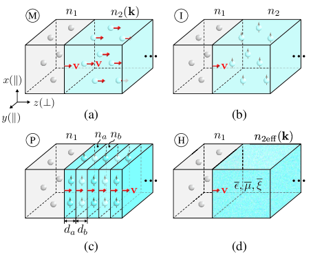
Figure 1: Dynamic systems considered in the paper. (a) Moving-matter bloc (M system). (b) Moving-perturbation interface (I system). (c) Moving-perturbation periodic (bilayer unit-cell) structure (P system). (d) Metamaterial homogenization of (c) (H system).

Figure 1(a) represents the structure of a moving-matter bloc (M system). This common dynamic system involves an object made of medium 2 (isotropic at rest with $n_{2}=\sqrt{\epsilon_{\mathrm{r}2}\mu_{\mathrm{r}2}}$), propelled by an external force and moves at the velocity of $\mathbf{v}$ in the background medium 1. The motion of molecules and atoms within medium 2 induces Fresnel-Fizeau drag, resulting in the transformation of its initial isotropic state into a bianisotropic medium described by $n_{2}(\mathbf{k})$ [10, 16]. Figure 1(b) illustrates the configuration of a moving-perturbation interface (I system). Unlike the moving-matter bloc, the interface of the system is formed by a traveling-wave modulation step. Therefore, there is no net motion of matter and only the perturbation (interface) moves. This system breaks the velocity limitation and can be both subluminal and superluminal, with the limiting case, where $v\rightarrow\infty$, corresponding to the pure-time modulation-interface system [17, 18, 21, 23, 24, 30, 31, 33, 34, 35]. Figure 1(c) shows a moving-perturbation periodic structure (P system). This system is created by a periodic modulation, composed of the bilayer unit-cell presented in Fig. 1(b). In the Bragg regime, where $d\approx\lambda_{\mathrm{i}}/2$, with $d=d_{a}+d_{b}$ representing the size of the unit cell and $\lambda_{\mathrm{i}}$ denoting the incident wavelength, multiple scatterings occur within each layer [29]; in the long-wavelength regime, where $d<<\lambda_{\mathrm{i}}$, as depicted in Fig. 1(d), the periodic structure can be homogenized as a bianisotropic medium with the effective refractive index of $n_{2\mathrm{eff}}(\mathbf{k})$ [48] (H system). The long-wavelength-regime periodic structure serves as the modulation counterpart to the modulation-type moving-matter material, which will be investigated in detail in this paper.

III Space-Time Homogenization and Fresnel-Fizeau Drag

In the long-wavelength regime, homogenization of the moving-perturbation periodic structure can simplify the media by representing them with effective parameters, such as the effective permittivity $\overline{\epsilon}$, permeability $\overline{\mu}$ and electromagnetic cross-coupling $\overline{\xi}$. Several space-time homogenization methods have been recently proposed in the literature. One of the most common ones is the frame-hopping method [15], which can be implemented either by employing Galilean transformation to the comoving frame $K^{\prime}$ with $c\rightarrow\infty$ [48, 53], or by using Lorentz transformation, maintaining $c$ as the speed of light in vacuum to ensure a physical transformation. In the case of Lorentz frame-hopping, transformation to the comoving frame ($v_{\mathrm{f}}=v$, where $v_{\mathrm{f}}$ is the velocity of the frame chosen for transformation) is realized in the subluminal regime [54, 32, 37], while transformation to the instantaneous frame ($v_{\mathrm{f}}=c^{2}/v$) is applied in the superluminal regime to avoid imaginary Lorentz factor $\gamma=1/\sqrt{1-(v_{\mathrm{f}}/c)^{2}}$ [29], as shown in Appendix A. Another method is the weighted-average method [29, 32], which involves averaging the wave velocity in the laboratory frame to determine the effective refractive index. This approach is also applicable for finding the band structures of space-time crystals in the Bragg regime [29]. However, it only yields the effective medium parameter for the refractive index under normal incidence condition, without providing information on $\overline{\epsilon}$, $\overline{\mu}$ and $\overline{\xi}$.

Figure 2 compares the averaged medium parameters obtained using the aforementioned homogenization methods. Two scenarios are considered: the case of impedance mismatch [Fig. 2(a)] and impedance match [Fig. 2(b)] for the two media composing the bilayers [Fig. 1(c)]. As shown in Fig. 2, the final homogenization results using Galilean and Lorentz frame-hopping methods are consistent in the laboratory frame $K$ [54], whereas the weighted-average method is only accurate in the case of impedance match (lack of reflection). This is because the weighted-average method is a velocity-average approximation, which is accurate when only one wave propagates in each layer.

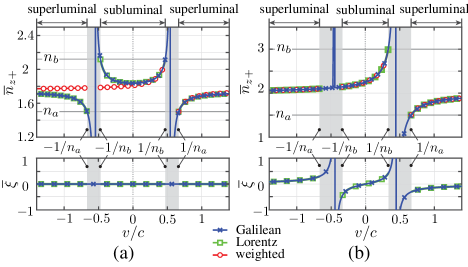
Figure 2: Comparison of the averaged refractive indices in the $+z$ direction $\overline{n}_{z+}$ (top panels) and cross-coupling parameters $\overline{\xi}$ (bottom panels) versus the normalized interface velocity $v/c$, utilizing Galilean and Lorentz frame-hopping homogenization methods and weighted-average method for a moving-perturbation periodic structure [Fig. 1(c) with $d_{a}=d_{b}$], in the scenarios of (a) impedance-mismatched media with $\epsilon_{\mathrm{r}a}=\mu_{\mathrm{r}a}=\mu_{\mathrm{r}b}=1.5$ and $\epsilon_{\mathrm{r}b}=3$, and (b) impedance-matched media with $\epsilon_{\mathrm{r}a}=\mu_{\mathrm{r}a}=1.5$ and $\epsilon_{\mathrm{r}b}=\mu_{\mathrm{r}b}=3$. The gray areas correspond to the interluminal regimes $|c/n_{b}|<|v|<|c/n_{a}|$ [48, 16].

The dispersion relation for bianisotropic media reads [10, 16]

$$\left|\omega^{2}\overline{\overline{\epsilon}}_{2}+(\overline{\overline{k}}+\omega\overline{\overline{\xi}}_{2})\cdot\overline{\overline{\mu}}_{2}^{-1}\cdot(\overline{\overline{k}}-\omega\overline{\overline{\zeta}}_{2})\right|=0,$$ (1a)

where

$$\overline{\overline{k}}=\left[\begin{array}[]{ccc}0&-k_{z}&k_{y}\\ k_{z}&0&-k_{x}\\ -k_{y}&k_{x}&0\end{array}\right].$$ (1b)

In the case of moving-matter bloc, the matter-motion-induced bianisotropic matrices are [16]

$$\begin{gathered}\overline{\overline{\epsilon}}_{2}=\epsilon_{2}\left[\begin{array}[]{lll}\alpha_{2}&0&0\\ 0&\alpha_{2}&0\\ 0&0&1\end{array}\right],\quad\overline{\overline{\mu}}_{2}=\mu_{2}\left[\begin{array}[]{lll}\alpha&0&0\\ 0&\alpha&0\\ 0&0&1\end{array}\right],\\ \overline{\overline{\xi}}_{2}=\left[\begin{array}[]{ccc}0&\xi_{2}&0\\ -\xi_{2}&0&0\\ 0&0&0\end{array}\right]\quad\text{and}\quad\overline{\overline{\zeta}}_{2}=-\overline{\overline{\xi}}_{2},\end{gathered}$$ (2a)

where $$\alpha_{2}=\frac{1-(v/c)^{2}}{1-(n_{2}v/c)^{2}} \xi_{2}=\frac{v}{c^{2}}\frac{1-n_{2}^{2}}{1-(n_{2}v/c)^{2}}$$ and . In the case of moving-perturbation interface, the second medium is stationary and isotropic [29] with

$$\overline{\overline{\epsilon}}_{2}=\epsilon_{2}\overline{\overline{\mathrm{I}}},\quad\overline{\overline{\mu}}_{2}=\mu_{2}\overline{\overline{\mathrm{I}}}\quad\textrm{and}\quad\overline{\overline{\xi}}_{2}=\overline{\overline{\zeta}}_{2}=\overline{\overline{\mathrm{O}}},$$ (2b)

where $$\overline{\overline{\mathrm{I}}} \overline{\overline{\mathrm{O}}} 3\times 3$$ and are the identity and null matrices, respectively. In the case of moving-perturbation periodic structure, employing the frame-hopping method (Appendix A), the media are homogenized as

$$\begin{gathered}\overline{\overline{\epsilon}}_{2}=\left[\begin{array}[]{lll}\overline{\epsilon}_{\|}&0&0\\ 0&\overline{\epsilon}_{\|}&0\\ 0&0&\overline{\epsilon}_{\perp}\end{array}\right],\quad\overline{\overline{\mu}}_{2}=\left[\begin{array}[]{lll}\overline{\mu}_{\|}&0&0\\ 0&\overline{\mu}_{\|}&0\\ 0&0&\overline{\mu}_{\perp}\end{array}\right],\\ \overline{\overline{\xi}}_{2}=\left[\begin{array}[]{ccc}0&\overline{\xi}&0\\ -\overline{\xi}&0&0\\ 0&0&0\end{array}\right]\quad\text{and}\quad\overline{\overline{\zeta}}_{2}=-\overline{\overline{\xi}}_{2}.\end{gathered}$$ (2c)

Figure 3 illustrates the isofrequency curves [Eqs. (1)] for the three systems in different velocity regimes. As shown in the figure, the conventional Fresnel-Fizeau drag, with drag in the direction of motion, is observed in the moving-matter bloc. The modulation interface system experiences no drag in all velocity regimes since the second medium is always isotropic. In the subluminal homogenized periodic system, reverse drag occurs; while in the superluminal regime, the drag direction remains the same as in the conventional case [29, 43], albeit with a smaller effective refractive index, as indicated by the radii of the curves in the figure.

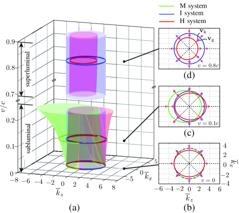
Figure 3: Isofrequency curves for moving-matter (M) system, moving-perturbation interface (I) system and homogenized periodic (H) system (a) in the comoving subluminal and superluminal regimes, along with specific cases at three different velocities: (b) $v=0$, (c) $v=0.1c$ and (d) $v=0.8c$. The M and I systems have the rest medium parameters $\epsilon_{\mathrm{r}1}=\mu_{\mathrm{r}1}=1.5$ and $\epsilon_{\mathrm{r}2}=\mu_{\mathrm{r}2}=3$ and the H system has the rest medium parameters $\epsilon_{\mathrm{r}1,b}=\mu_{\mathrm{r}1,b}=1.5$, $\epsilon_{\mathrm{r}a}=\mu_{\mathrm{r}a}=4.5$ with $d_{a}=d_{b}$ [Fig. 1(c)].

IV General Formulation for Scattering
at Dynamic Discontinuities

The scattering problem at different dynamic discontinuities shown in Fig. 1 can be conceptualized as a general scattering problem at a moving discontinuity separating an isotropic medium and a bianisotropic medium. The specific medium parameters for the three dynamic systems are provided in Eqs. (2). In this section, we will introduce the general formulas governing the frequency transitions and scattering coefficients.

The frequency relations between the scattered waves and incident wave are derived by transforming to the comoving frame in the subluminal regime, where the interfaces are purely spatial and the frequency is conserved ($\omega^{\prime}_{\mathrm{i}}=\omega^{\prime}_{\mathrm{r}}=\omega^{\prime}_{\mathrm{t}}$), and to the instantaneous frame in the superluminal regime, where the interfaces are purely temporal and the momentum is conserved ($k^{\prime}_{\mathrm{i}}=k^{\prime}_{\zeta}=k^{\prime}_{\xi}$). Then, transforming the conserved values back to the $K$ frame using Lorentz transformations $\omega^{\pm\prime}=\gamma(\omega^{\pm}\mp v_{\mathrm{f}}k^{\pm})$ and $k^{\pm\prime}=\gamma(k^{\pm}\mp v_{\mathrm{f}}\omega^{\pm}/c^{2})$ [29, 10], we find the subluminal frequency transition relations as

$$\omega_{\mathrm{r}}=\omega_{\mathrm{i}}\frac{1-n_{1}v/c}{1+n_{1}v/c}\quad\textrm{and}\quad\omega_{\mathrm{t}}=\omega_{\mathrm{i}}\frac{1-n_{1}v/c}{1-n_{2+}v/c},$$ (3)

and the superluminal relations as

$$\omega_{\zeta}=\omega_{\mathrm{i}}\frac{1-n_{1}v/c}{1+n_{2-}v/c}\quad\textrm{and}\quad\omega_{\xi}=\omega_{\mathrm{i}}\frac{1-n_{1}v/c}{1-n_{2+}v/c},$$ (4)

with the (effective) refractive indices of the second medium in the $\pm z$ directions given by the formula [16]

$$n_{2\pm}=c(\sqrt{\epsilon_{2\|}\mu_{2\|}}\pm\xi_{2}),$$ (5)

derived in Appendix B.

We derive the scattering coefficients directly in the $K$ frame from the moving boundary conditions [15, 57]

$$\mathbf{E}_{1\|}+\mathbf{v}\times\mathbf{B}_{1\|} =\mathbf{E}_{2\|}+\mathbf{v}\times\mathbf{B}_{2\|},$$ (6a)

$$\mathbf{H}_{1\|}-\mathbf{v}\times\mathbf{D}_{1\|} =\mathbf{H}_{2\|}-\mathbf{v}\times\mathbf{D}_{2\|}.$$ (6b)

Eliminating all the field quantities, we obtain the subluminal reflection coefficient $r$ and transmission coefficient $t$ as (see detailed derivations in Appendix B)

$$r=\frac{\eta_{2}-\eta_{1}}{\eta_{1}+\eta_{2}}\frac{1-n_{1}v/c}{1+n_{1}v/c}\quad\textrm{and}\quad t=\frac{2\eta_{2}}{\eta_{1}+\eta_{2}}\frac{1-n_{1}v/c}{1-n_{2+}v/c},$$ (7)

and the superluminal backward coefficient $\zeta$ and forward coefficient $\xi$ as

$$\zeta=\frac{\eta_{1}-\eta_{2}}{2\eta_{1}}\frac{1-n_{1}v/c}{1+n_{2-}v/c}\quad\textrm{and}\quad\xi=\frac{\eta_{1}+\eta_{2}}{2\eta_{1}}\frac{1-n_{1}v/c}{1-n_{2+}v/c},$$ (8)

where

$$\eta_{1}=\sqrt{\frac{\mu_{1}}{\epsilon_{1}}}\quad\textrm{and}\quad\eta_{2}=\sqrt{\frac{\mu_{2\|}}{\epsilon_{2\|}}}\$$ (9)

are the wave impedances of the two media (Appendix B).

Figure 4 compares the scattering of a normally incident modulated Gaussian pulse at an actual moving-perturbation periodic structure with its homogenized counterpart, based on full-wave (FDTD) simulation results [57, 58]. We consider here a subluminal velocity in Fig. 4(a) and a superluminal velocity in Fig. 4(b). The left panels illustrate the scattering phenomena at a specific time after interacting with the interfaces. The right panels provide quantitative validations in terms of the Fourier-transformed field distributions, where the circles correspond to the analytical results [Eqs. (3), (4), (7) and (8)] for the pulse central frequency. As shown in Fig. 4, despite the homogenization approximation considered in the derivations of the analytical results for the moving-perturbation periodic structure, the results exhibit a good agreement with the actual scattering and we will therefore use this model in the rest of this paper.

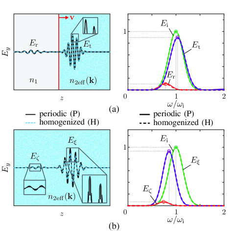
Figure 4: Full-wave simulated (FDTD) results for the scattering of the modulated Gaussian pulse at a periodic and homogenized moving-perturbation structure with $\epsilon_{\mathrm{r}1}=1.5$, $\epsilon_{\mathrm{r}2}=3$ and $\mu_{\mathrm{r}1}=\mu_{\mathrm{r}2}=1$, moving at (a) the subluminal velocity, $v=0.1c$ and (b) the superluminal velocity $v=10c$. In both cases, the unit-cell size is set to $d=\lambda_{\mathrm{i}}/10$ with $d_{a}=d_{b}$ [Fig. 1(c)]. The left panels showcase snapshots capturing the scattering waves after interacting with the modulation interfaces and the right panels present the Fourier transforms of the scattered and incident pulses. The insets in the left panels showcase the waveforms in the periodic structures.

V Generalized Energy-Momentum
Conservation Laws

We shall now generalize the electromagnetic energy-momentum conservation laws, already formulated for moving-matter systems in [5], to encompass the moving-perturbation interface and homogenized periodic structure systems (Fig. 1). This will be accomplished with the help of Fig. 5, which shows a moving cylindrical volume, $\mathcal{V}=\mathcal{V}(z,t)$, defined by the closed surface $\mathcal{S}=\mathcal{S}(z,t)$ with outward pointing normal unit vector $\hat{\mathbf{n}}$, positioned across the two media, and moving together with the discontinuity at the velocity $\mathbf{v}$.

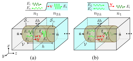
Figure 5: Imaginary cylinder moving with the dynamic discontinuity whose velocity is in the comoving ($v>0$) (a) subluminal regime and (b) superluminal regime. The top panels showcase the corresponding moving refractive index steps.

The conservation law for the energy may be expressed as [11, 10]

$$\iiint\frac{\partial W}{\partial t}~{}\mathrm{d}\mathcal{V}=-\oiint\mathbf{S}\cdot\hat{\mathbf{n}}~{}\mathrm{d}\mathcal{S}+\iiint p~{}\mathrm{d}\mathcal{V},$$ (10a)

where $$W=(\mathbf{D}\cdot\mathbf{E}+\mathbf{B}\cdot\mathbf{H})/2 \mathbf{S}=\mathbf{E}\times\mathbf{H} p p>0 p<0 \mathcal{V} \mathcal{S} \mathcal{V}$$ is the energy density of the wave, is the corresponding Poynting vector and is the power density gain () or loss () of an external source, which is here the source of the motion, viz., a mechanical force (M system), a step perturbation modulation (I system) or a periodic perturbation modulation (P and H systems). Equation (10a) means that the temporal variation of the wave energy in is equal to the sum of the wave power flux through into and the power transferred by the external source to the wave.

Similarly, the conservation law for the momentum may be expressed as [11, 10]

$$\iiint\frac{\partial\mathbf{g}}{\partial t}~{}\mathrm{d}\mathcal{V}=-\oiint\overline{\overline{\mathrm{T}}}\cdot\hat{\mathbf{n}}~{}\mathrm{d}\mathcal{S}+\iiint\mathbf{f}~{}\mathrm{d}\mathcal{V},$$ (10b)

where $\mathbf{g}=\mathbf{D}\times\mathbf{B}$ is the momentum density of the wave, $\overline{\overline{\mathrm{T}}}=\frac{1}{2}(\mathbf{D}\cdot\mathbf{E}+\mathbf{B}\cdot\mathbf{H})\overline{\overline{\mathrm{I}}}-\mathbf{D}\mathbf{E}-\mathbf{B}\mathbf{H}$ is the corresponding Maxwell stress tensor and $\mathbf{f}$ is the force density related to $p$ ($p=\mathbf{v}\cdot\mathbf{f}$) in Eq. (10a). Equation (10b) means that the temporal variation of the wave momentum in $\mathcal{V}$ is equal to the sum of the wave force flux through $\mathcal{S}$ into $\mathcal{V}$ and the momentum transferred by the external source to the wave.

Equations (10) may be rewritten, for later simplification, in terms of total (as opposed to partial) time derivatives with the help of the general Leibniz integral rule, or Reynolds transport theorem [5, 59, 60],

$$\frac{\mathrm{d}}{\mathrm{d}t}\iiint A~{}\mathrm{d}\mathcal{V}=\iiint\frac{\partial A}{\partial t}~{}\mathrm{d}\mathcal{V}+\oiint A~{}\mathbf{v}\cdot\hat{\mathbf{n}}~{}\mathrm{d}\mathcal{S},$$ (11)

where $A=A(x,y,z,t)$ may be either a scalar or vector. Using Eq. (11) with $A$ replaced by $W$ and $\mathbf{g}$ in Eqs. (10a) and (10b), respectively, yields the new conservation laws

$$\iiint p~{}\mathrm{d}\mathcal{V}=\frac{\mathrm{d}}{\mathrm{d}t}\iiint W~{}\mathrm{d}\mathcal{V}+\oiint(\mathbf{S}-W\mathbf{v})\cdot\hat{\mathbf{n}}~{}\mathrm{d}\mathcal{S}$$ (12a)

and

$$\iiint\mathbf{f}~{}\mathrm{d}\mathcal{V}=\frac{\mathrm{d}}{\mathrm{d}t}\iiint\mathbf{g}~{}\mathrm{d}\mathcal{V}+\oiint\left(\overline{\overline{\mathrm{T}}}-\mathbf{g}\mathbf{v}\right)\cdot\hat{\mathbf{n}}~{}\mathrm{d}\mathcal{S}.$$ (12b)

We may alternatively write the integral formulas (12) into their local forms by reducing the cylinder in Fig. 5 to an infinitesimally thin pillbox, of thickness $h=\delta{h}\rightarrow{0}$, as

$$\lim_{\delta h\rightarrow 0}\iiint p~{}\mathrm{d}\mathcal{V}=\lim_{\delta h\rightarrow 0}\oiint(\mathbf{S}-W\mathbf{v})\cdot\hat{\mathbf{n}}~{}\mathrm{d}\mathcal{S}$$ (13a)

and

$$\lim_{\delta h\rightarrow 0}\iiint\mathbf{f}~{}\mathrm{d}\mathcal{V}=\lim_{\delta h\rightarrow 0}\oiint\left(\overline{\overline{\mathrm{T}}}-\mathbf{g}\mathbf{v}\right)\cdot\hat{\mathbf{n}}~{}\mathrm{d}\mathcal{S},$$ (13b)

where time derivative expressions in Eqs. (12) have disappeared because the related integrals can only be constant in time since the velocity of the interface is itself constant in time and since we will ultimately consider time-averaged harmonic waves (see Sec. VI). Finally, using the relations

$$\lim_{\delta h\rightarrow 0}\iiint A~{}\mathrm{d}\mathcal{V}=\lim_{\delta h\rightarrow 0}\iint\left(\int_{\delta h}A~{}\mathrm{d}h\right)\mathrm{d}\mathcal{S}=\iint A_{\mathrm{s}}~{}\mathrm{d}\mathcal{S},$$ (14a)

where $$A_{\mathrm{s}}=A\delta h$$, and

$$\lim_{\delta h\rightarrow 0}\oiint A~{}\mathrm{d}\mathcal{S}=\iint\left(A_{+}-A_{-}\right)\mathrm{d}\mathcal{S},$$ (14b)

where $A_{\pm}$ represents the value of $A$ on the $\mathcal{S}_{\pm}$ surface, we may write Eqs. (13) in their local-differential forms,

$$p_{\mathrm{s}}=\hat{\mathbf{n}}\cdot[\mathbf{S}]-v[W]$$ (15a)

and

$$\mathbf{f}_{\mathrm{s}}=\hat{\mathbf{n}}\cdot[\overline{\overline{\mathrm{T}}}]-v[\mathbf{g}],$$ (15b)

where $$[A]=A_{+}-A_{-} A p_{\mathrm{s}}=p\delta{h} \mathbf{f}_{\mathrm{s}}=\mathbf{f}\delta h p \mathbf{f}$$ denotes the difference of across the discontinuity, and and are the surface power and force densities corresponding to the and .

Equations (15) are the key general formulas of the paper, which may be interpreted in terms of wave-medium interactions as follows: In the absence of dissipation, $p_{\mathrm{s}}$ represents the power (surface density) transferred by the modulation to the wave when $p_{\mathrm{s}}>0$, or removed from the wave when $p_{\mathrm{s}}<0$; while $\mathbf{f}_{\mathrm{s}}$ represents the force (surface density) exerted by the modulation onto the wave when $\mathbf{f}_{\mathrm{s}}>0$, or exerted onto the modulation by the wave when $\mathbf{f}_{\mathrm{s}}<0$.

VI Analysis and Discussion

We shall restrict our attention to harmonic waves, for which the quantities $p_{\mathrm{s}}$ and $\mathbf{f}_{\mathrm{s}}$ in Eqs. (15) can easily be expressed in terms of the structural parameters $\eta$, $n$ and $v$, and for which we may conveniently use time averages, denoted as $\langle\cdot\rangle$, in Eqs. (15). The related derivations are given in Appendix C.

As suggested by the inset above the figures in Fig. 5, the scattering phenomenology is quite different in the subluminal and superluminal cases. In both cases, incidence occurs in medium 1 and transmission occurs in medium 2. However, reflection occurs in media 1 and 2 for the subluminal and superluminal cases, respectively. The situation of the subluminal (space-like) case [Fig. 5(a)] is easily understandable, as it is similar to scattering at a spatial discontinuity, with reflection occurring on the same side as incidence. The superluminal (time-like) case [Fig. 5(b)], being similar to a temporal discontinuity with later forward and later backward waves [27], is less intuitive. Medium 1 must then be placed at the right (farther along $z$) of medium 2, for otherwise the wave, being slower than the interface, would never catch the interface and there would be no scattering, a situation without interest; in contrast, with medium 1 on the right, the wave gets overtaken by the interface, and interesting scattering occurs.

Substituting the scattering coefficients (7) and (8) into Eq. (15a) and eliminating all the field quantities, we obtain the time-averaged power transfer density $\langle p_{\mathrm{s}}\rangle$ for the co/contra-moving ($\pm$) subluminal (sub$\pm$) and superluminal regimes (sup$\pm$) at the moving discontinuity surface as (see Appendix C)

$$\begin{split}\langle p_{\mathrm{s}}^{{\mathrm{sub}\pm}}\rangle=I_{\mathrm{i}}\Bigg{[}\frac{\eta_{1}}{\eta_{2}}\Bigg{(}1-&\frac{n_{2+}v}{c}\Bigg{)}t^{2}\\ &+\Bigg{(}1+\frac{n_{1}v}{c}\Bigg{)}r^{2}-\Bigg{(}1-\frac{n_{1}v}{c}\Bigg{)}\Bigg{]}\end{split}$$ (16a)

and

$$\begin{split}\langle p_{\mathrm{s}}^{\mathrm{sup}\pm}\rangle=\pm I_{\mathrm{i}}\Bigg{\{}-\frac{\eta_{1}}{\eta_{2}}\Bigg{[}\Bigg{(}1-\frac{n_{2+}v}{c}\Bigg{)}\xi^{2}-\Bigg{(}1+\frac{n_{2-}v}{c}\Bigg{)}\zeta^{2}\Bigg{]}&\\ +\Bigg{(}1-\frac{n_{1}v}{c}\Bigg{)}\Bigg{\}},&\end{split}$$ (16b)

where $$I_{\mathrm{i}}=E_{\mathrm{i}}^{2}/(2\eta_{1})=(E_{\mathrm{i}}^{2}/2)\sqrt{\epsilon_{1}/\mu_{1}}$$ is the incident field intensity.

For simplicity, we consider the impedance-matched case, where $\eta_{2}=\eta_{1}$ and hence $r=\zeta=0$. Substituting Eqs. (7) and (8) into Eqs. (16a) and (16b), respectively, we obtain

$$|\langle p_{\mathrm{s}}\rangle|=I_{\mathrm{i}}\Bigg{|}\Bigg{(}1-\frac{n_{1}v}{c}\Bigg{)}\Bigg{[}\frac{1}{1-n_{2+}v/c}-\Bigg{(}1-\frac{n_{1}v}{c}\Bigg{)}\Bigg{]}\Bigg{|}.$$ (17)

Fig. 6 illustrates the magnitude of the surface power transfer density $|\langle\overline{p}_{\mathrm{s}}\rangle|$ [Eq. (17)] versus the interface velocity $v$ and the refractive index contrast $\Delta n=n_{2+}-n_{1}$. As shown in the figure, $|\langle\overline{p}_{\mathrm{s}}\rangle|$ is proportional to both $|v|$ and $\Delta n$, which indicates that faster velocity and higher contrast result in increased power loss or gain, and vice versa.

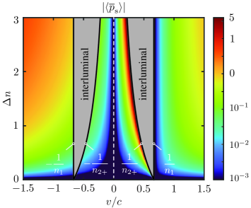
Figure 6: Normalized time-averaged surface power transfer density $|\langle\overline{p}_{\mathrm{s}}\rangle|=|\langle p_{\mathrm{s}}\rangle/I_{\mathrm{i}}|$ [Eq. (17)] versus the normalized interface velocity $v/c$ and the refractive index contrast $\Delta n=n_{2+}-n_{1}$ with $n_{1}=1.5$ and $\eta_{2}=\eta_{1}$ (impedance-matched case). The gray areas correspond to the interluminal regimes $|c/n_{2+}|<|v|<|c/n_{1}|$.

Figure 7 compares the surface power transfer density [Eqs. (16)] for the three systems in different velocity regimes. Again, all three systems use the same rest-frame medium parameters as those shown in Fig. 3. Dashed areas in Fig. 7 denote interluminal regimes, encompassing phenomena such as Čerenkov radiation and unknown scattering [10, 8], which are beyond the scope of this paper. Note that the interluminal regimes differ among systems. In the case of the moving-perturbation periodic structure involving three media [Fig. 1(c)], the interluminal velocity regime is characterized by $|\min(c/n_{1},c/n_{a},c/n_{b})|<|v|<|\max(c/n_{1},c/n_{a},c/n_{b})|$. In contrast, for the systems involving only two media, such as matter and interface systems [Figs. 1(a) and (b)], the velocity regime is $|\min(c/n_{1},c/n_{2})|<|v|<|\max(c/n_{1},c/n_{2})|$.

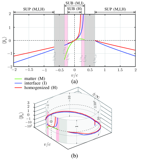
Figure 7: Normalized time-averaged surface power transfer density $\langle\overline{p}_{\mathrm{s}}\rangle=\langle p_{\mathrm{s}}\rangle/I_{\mathrm{i}}$ versus the normalized interface velocity $v/c$ for different dynamic systems with plotting on (a) a flat plane and (b) a cylinder surface. The media parameters are the same as those in Fig. 3. Log scale is used in Fig. 7(b) for $\langle\overline{p}_{\mathrm{s}}\rangle<-1$ and $|v/c|>1$ to show the limiting case of $v\rightarrow\pm\infty$.

Several observations and explanations are in order regarding Fig. 7. A global observation is that moving-perturbation system may achieve the same power transfer as the moving-matter system by adjusting the modulation velocity. While minor power transfers can often be disregarded, significant power transfers may impact the total modulation power supply. The limiting case of $v\rightarrow\pm\infty$ corresponds to the pure-time systems, featuring an infinite exchange power limitation, as shown in Fig. 7(b), which indicates that the sharp temporal modulation step is not physical.

Specifically, in a horizontal analysis of Fig. 7(a) examining different velocities, two key phenomena can be identified: the frequency transition at the microscopic level and the “catch-up” effect [29, 27, 36] at the macroscopic level. At the microscopic level, the varying degrees of frequency transitions for each photon interacting with the moving discontinuity at different velocities are essential for grasping the dynamics of wave-particle interactions, leading to diverse energy exchanges. On the macroscopic scale, the “catch-up” effect, involving the “smashing” and “cushioning” of the wave against the moving discontinuity, is significant. This effect is particularly notable as the velocity of the discontinuity approaches that of the wave, exerting a considerable influence on power transfer mechanism with $|p_{\mathrm{s}}|\rightarrow\infty$. In a vertical analysis of Fig. 7(a), where a given velocity is considered across different systems, a determinant phenomenon is the Fresnel-Fizeau drag, as depicted in Fig. 3. Despite the interface velocity remaining constant, different systems exhibit varying levels of interaction due to differences in the effective refractive index $n_{2+}$ of the second medium. In the subluminal regime, this interaction is most pronounced in the homogenized moving-perturbation periodic system, where the opposite drag resulting in largest refractive index contrast $\Delta n=n_{2+}-n_{1}$, and, in contrast, least significant in the moving-matter bloc (see Table VI and Fig 6). A similar explanation applies to the superluminal regime.

TABLE I: Comparison of the three systems in the comoving subluminal case

c——c—c—c fixed $n_{1}$ & M I H
Fresnel-Fizeau drag $>0$ [1, 2] $0$ $<0$ [43, 29]
wave velocity in the $+z$-direction $v_{2+}$ $\nearrow$ $-$ $\searrow$
refractive index $n_{2+}=c/v_{2+}$ $\searrow$ $-$ $\nearrow$
refractive index contrast $\Delta n=n_{2+}-n_{1}$ $\searrow$ $-$ $\nearrow$
surface power and force density $\langle p_{\mathrm{s}}\rangle$, $\langle f_{\mathrm{s}}\rangle$ $\searrow$ $-$ $\nearrow$

Similarly, substituting the scattering coefficients (7) and (8) into Eq. (15b) and eliminating all the field quantities, we obtain the time-averaged force density $\langle f_{\mathrm{s}}\rangle$ at the moving discontinuity surface as (see Appendix C)

$$\begin{split}\langle f_{\mathrm{s}}^{\mathrm{sub}\pm}\rangle=\frac{I_{\mathrm{i}}}{c}\Bigg{[}\frac{\eta_{1}n_{2+}}{\eta_{2}}\Bigg{(}1-\frac{n_{2+}v}{c}\Bigg{)}t^{2}&-n_{1}\Bigg{(}1+\frac{n_{1}v}{c}\Bigg{)}r^{2}\\ &-n_{1}\Bigg{(}1-\frac{n_{1}v}{c}\Bigg{)}\Bigg{]}\end{split}$$ (18a)

and

$$\begin{split}\langle f_{\mathrm{s}}^{\mathrm{sup}\pm}\rangle=&\pm\frac{I_{\mathrm{i}}}{c}\Bigg{[}-\frac{\eta_{1}n_{2+}}{\eta_{2}}\Bigg{(}1-\frac{n_{2+}v}{c}\Bigg{)}\xi^{2}\\ &-\frac{\eta_{1}n_{2-}}{\eta_{2}}\Bigg{(}1+\frac{n_{2-}v}{c}\Bigg{)}\zeta^{2}+n_{1}\Bigg{(}1-\frac{n_{1}v}{c}\Bigg{)}\Bigg{]}.\end{split}$$ (18b)

Figure 8 compares the surface force density [Eqs. (18)] for the three systems in different velocity regimes, utilizing the same media parameters as depicted in Fig. 7. As illustrated in Fig. 8(b), unlike the power transfer curves (Fig. 7), the forces in the limiting cases of $v\rightarrow\infty$ and $v\rightarrow-\infty$ exhibit opposite signs. This indicates that the force acts in both $+z$ and $-z$ directions at the limit, resulting in a net force of zero, since there is no spatial variation involved in the limiting pure-time case [56, 34]. Various factors, including the “smashing” and “cushioning” effect, as well as the Fresnel-Fizeau drag, also influence the momentum dynamics in different velocity regimes and systems.

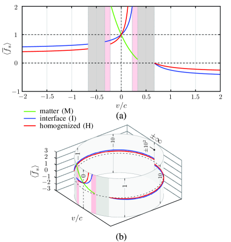
Figure 8: Normalized time-averaged surface force density $\langle\overline{f}_{\mathrm{s}}\rangle=\langle f_{\mathrm{s}}\rangle/\langle f_{0}\rangle$ (where $\langle f_{0}\rangle$ is the rest surface force density with $v=0$) versus the normalized interface velocity $v/c$ for different dynamic systems with plotting on (a) a flat plane and (b) a cylinder surface. The media parameters remain consistent with those depicted in Fig. 7. Log scale is used in Fig. 8(b) for $|v/c|>1$.

VII Conclusion

This work has filled a critical gap in understanding scattering and energy-momentum relations in dynamic systems. Deriving general solutions and analyzing energy-momentum relations, we have provided insights into the wave-medium interaction behavior. Our analysis encompasses a comparison of different dynamic systems, shedding light on their unique characteristics and performance similarities. Moving forward, it is imperative to consider practical implementations of modulation systems. Utilizing switched transmission-line [33], free-carrier injection [28] and other modulation techniques [26, 32], we must account for extreme power transfer scenarios and their implications. By integrating these considerations into system design and operation, we can enhance performance and optimize outcomes across diverse applications.

Appendix A Frame-Hopping Space-Time Homogenization Method Using Lorentz Transformation

We derive here the homogenized medium parameters for the moving-perturbation periodic structure in both subluminal and superluminal regimes. Although in the subluminal case, the basic formulas are already given in Refs. [54, 32] and [37] (assuming zero acceleration $a^{\prime}=0$ for uniform velocity), we re-derive them here for the sake of completeness and notational convenience.

We first provide here the fields Lorentz transformations [10], which will be used later:

$$\mathbf{E}_{\|}^{\prime}=\gamma\left(\mathbf{E}_{\|}+\mathbf{v}_{\mathrm{f}}\times\mathbf{B}_{\|}\right),$$ (19a)

$$\mathbf{B}_{\|}^{\prime}=\gamma\left(\mathbf{B}_{\|}-\frac{1}{c^{2}}\mathbf{v}_{\mathrm{f}}\times\mathbf{E}_{\|}\right),$$

$$\mathbf{E}_{\perp}^{\prime}=\mathbf{E}_{\perp},$$

$$\mathbf{B}_{\perp}^{\prime}=\mathbf{B}_{\perp},$$

and

$$\mathbf{H}_{\|}^{\prime} =\gamma\left(\mathbf{H}_{\|}-\mathbf{v}_{\mathrm{f}}\times\mathbf{D}_{\|}\right),$$ (19b)

$$\mathbf{D}_{\|}^{\prime} =\gamma\left(\mathbf{D}_{\|}+\frac{1}{c^{2}}\mathbf{v}_{\mathrm{f}}\times\mathbf{H}_{\|}\right),$$

$$\mathbf{H}_{\perp}^{\prime} =\mathbf{H}_{\perp},$$

$$\mathbf{D}_{\perp}^{\prime} =\mathbf{D}_{\perp},$$

where $$\boldsymbol{\psi}_{\|}=[\psi_{x}~{}\psi_{y}~{}0]^{\mathrm{T}} \boldsymbol{\psi}_{\perp}=[0~{}0~{}\psi_{z}]^{\mathrm{T}} \psi=E,H,D,B \mathbf{v}_{\mathrm{f}}=[0~{}0~{}v_{\mathrm{f}}]^{\mathrm{T}} \gamma=1/\sqrt{1-(v_{\mathrm{f}}/c)^{2}}$$, (), and .

A-A Subluminal Regime

Figure 9 illustrates the moving-perturbation periodic structure in the $K^{\prime}$ frame for the subluminal [Fig. 9(a)] and superluminal [Fig. 9(b)] regimes, along with the conserved field quantities at each discontinuity.

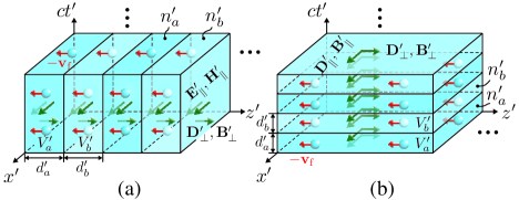
Figure 9: Space-time diagrams showcasing the conserved fields at each boundary in the $K^{\prime}$ frame for a moving-perturbation periodic structure in (a) the subluminal regime (space-like) and (b) the superluminal regime (time-like). The subscripts $\|$ and $\perp$ denote the spatial longitudinal and normal directions with respect to the interfaces in the $K$ frame (see Fig. 1) and do not refer to the directions relative to the temporal interfaces.

In the subluminal regime, the frame velocity $\mathbf{v}_{\mathrm{f}}$ is set equal to $\mathbf{v}$ in Eqs. (19), which corresponds to the comoving frame of the interfaces. As depicted in Fig. 9(a), in this comoving frame, the interfaces are stationary, while the atoms and molecules in media $a$ and $b$ move at the velocity of $-\mathbf{v}_{\mathrm{f}}$ relative to the interfaces, with the motion-induced bianisotropy constitutive relations given by [10, 16]

$$\mathbf{D}^{\prime}_{a,b}=\overline{\overline{\epsilon}}^{\prime}_{a,b}\cdot\mathbf{E}^{\prime}_{a,b}+\overline{\overline{\xi}}^{\prime}_{a,b}\cdot\mathbf{H}^{\prime}_{a,b},$$ (20a)

$$\mathbf{B}^{\prime}_{a,b}=\overline{\overline{\mu}}^{\prime}_{a,b}\cdot\mathbf{H}^{\prime}_{a,b}-\overline{\overline{\xi}}^{\prime}_{a,b}\cdot\mathbf{E}^{\prime}_{a,b},$$

where

$$\begin{gathered}\overline{\overline{\epsilon}}^{\prime}_{a,b}=\epsilon_{a,b}\left[\begin{array}[]{lll}\alpha^{\prime}_{a,b}&0&0\\ 0&\alpha^{\prime}_{a,b}&0\\ 0&0&1\end{array}\right]=\left[\begin{array}[]{lll}\epsilon^{\prime}_{a,b\|}&0&0\\ 0&\epsilon^{\prime}_{a,b\|}&0\\ 0&0&\epsilon^{\prime}_{a,b\perp}\end{array}\right],\\ \overline{\overline{\mu}}^{\prime}_{a,b}=\mu_{a,b}\left[\begin{array}[]{lll}\alpha^{\prime}_{a,b}&0&0\\ 0&\alpha^{\prime}_{a,b}&0\\ 0&0&1\end{array}\right]=\left[\begin{array}[]{lll}\mu^{\prime}_{a,b\|}&0&0\\ 0&\mu^{\prime}_{a,b\|}&0\\ 0&0&\mu^{\prime}_{a,b\perp}\end{array}\right],\\ \overline{\overline{\xi}}^{\prime}_{a,b}=\left[\begin{array}[]{ccc}0&\xi^{\prime}_{a,b}&0\\ -\xi^{\prime}_{a,b}&0&0\\ 0&0&0\end{array}\right],\end{gathered}$$ (20b)

with

$$\alpha^{\prime}_{a,b}=\frac{1-(v_{\mathrm{f}}/c)^{2}}{1-(n_{a,b}v_{\mathrm{f}}/c)^{2}}\quad\textrm{and}\quad\xi^{\prime}_{a,b}=-\frac{v_{\mathrm{f}}}{c^{2}}\frac{1-n_{a,b}^{2}}{1-(n_{a,b}v_{\mathrm{f}}/c)^{2}}.$$ (20c)

In the $K^{\prime}$ frame, the pure-space boundary conditions are [27]

$$\begin{gathered}\mathbf{E}^{\prime}_{a\|}=\mathbf{E}^{\prime}_{b\|}=\mathbf{E}^{\prime}_{\|},\quad\mathbf{H}^{\prime}_{a\|}=\mathbf{H}^{\prime}_{b\|}=\mathbf{H}^{\prime}_{\|},\\ \mathbf{D}^{\prime}_{a\perp}=\mathbf{D}^{\prime}_{b\perp}=\mathbf{D}^{\prime}_{\perp},\quad\mathbf{B}^{\prime}_{a\perp}=\mathbf{B}^{\prime}_{b\perp}=\mathbf{B}^{\prime}_{\perp}.\end{gathered}$$ (21)

Upon averaging the non-conserved field quantities $\mathbf{D}^{\prime}_{\|}$ and $\mathbf{E}^{\prime}_{\perp}$ at the interfaces,

$$\overline{\mathbf{D}}^{\prime}_{\|} =\frac{\int_{V^{\prime}_{a}}\mathbf{D}^{\prime}_{a\|}\mathrm{d}V^{\prime}+\int_{V^{\prime}_{b}}\mathbf{D}^{\prime}_{b\|}\mathrm{d}V^{\prime}}{V^{\prime}_{a}+V^{\prime}_{b}}$$ (22a)

$$=f(\epsilon^{\prime}_{a\|}\mathbf{E}^{\prime}_{\|}+\xi^{\prime}_{a}\mathbf{u}_{\|}\cdot\mathbf{H}^{\prime}_{\|})+(1-f)(\epsilon^{\prime}_{b\|}\mathbf{E}^{\prime}_{\|}+\xi^{\prime}_{b}\mathbf{u}_{\|}\cdot\mathbf{H}^{\prime}_{\|})$$

$$=[f\epsilon^{\prime}_{a\|}+(1-f)\epsilon^{\prime}_{b\|}]~{}\mathbf{E}^{\prime}_{\|}+[f\xi^{\prime}_{a}+(1-f)\xi^{\prime}_{b}]\mathbf{u}_{\|}\cdot\mathbf{H}^{\prime}_{\|}$$

$$=\overline{\epsilon}^{\prime}_{\|}\mathbf{E}^{\prime}_{\|}+\overline{\xi}^{\prime}\mathbf{u}_{\|}\cdot\mathbf{H}^{\prime}_{\|}$$

and

$$\overline{\mathbf{E}}^{\prime}_{\perp} =\frac{\int_{V^{\prime}_{a}}\mathbf{E}^{\prime}_{a\perp}\mathrm{d}V^{\prime}+\int_{V^{\prime}_{b}}\mathbf{E}^{\prime}_{b\perp}\mathrm{d}V^{\prime}}{V^{\prime}_{a}+V^{\prime}_{b}}$$ (22b)

$$=f(\mathbf{D}^{\prime}_{\perp}/\epsilon^{\prime}_{a\perp})+(1-f)(\mathbf{D}^{\prime}_{\perp}/\epsilon^{\prime}_{b\perp})$$

$$=\left(\frac{f}{\epsilon^{\prime}_{a\perp}}+\frac{1-f}{\epsilon^{\prime}_{b\perp}}\right)\mathbf{D}^{\prime}_{\perp}$$

$$=\overline{\epsilon}^{\prime-1}_{\perp}\mathbf{D}^{\prime}_{\perp},$$

where $$\mathbf{u}_{\|}=\left[\begin{array}[]{ccc}0&1&0\\ -1&0&0\\ 0&0&0\end{array}\right] f=d_{a}/(d_{a}+d_{b}) a$$ and is the proportion of medium [Fig, 1(c)],

and applying similar operations for $\mathbf{B}^{\prime}_{\|}$ and $\mathbf{H}^{\prime}_{\perp}$, we obtain the averaged parameters

$$\begin{gathered}\overline{\epsilon}^{\prime}_{\|}=f\epsilon^{\prime}_{a\|}+(1-f)\epsilon^{\prime}_{b\|},\\ \overline{\mu}^{\prime}_{\|}=f\mu^{\prime}_{a\|}+(1-f)\mu^{\prime}_{b\|},\\ \overline{\xi}^{\prime}=f\xi^{\prime}_{a}+(1-f)\xi^{\prime}_{b},\\ \overline{\epsilon}^{\prime}_{\perp}=\left(\frac{f}{\epsilon^{\prime}_{a\perp}}+\frac{1-f}{\epsilon^{\prime}_{b\perp}}\right)^{-1}\quad\textrm{and}\quad\overline{\mu}^{\prime}_{\perp}=\left(\frac{f}{\mu^{\prime}_{a\perp}}+\frac{1-f}{\mu^{\prime}_{b\perp}}\right)^{-1}.\end{gathered}$$ (23)

We may write the homogenized constitutive relations in the $K^{\prime}$ frame as

$${\left[\begin{array}[]{c}\overline{\mathbf{D}}^{\prime}_{\|}\\ \overline{\mathbf{B}}^{\prime}_{\|}\end{array}\right]} =\left[\begin{array}[]{cc}\overline{\epsilon}^{\prime}_{\|}&\overline{\xi}^{\prime}\\ -\overline{\xi}^{\prime}&\overline{\mu}^{\prime}_{\|}\end{array}\right]\left[\begin{array}[]{c}\overline{\mathbf{E}}^{\prime}_{\|}\\ \overline{\mathbf{H}}^{\prime}_{\|}\end{array}\right],$$ (24a)

$$\overline{\mathbf{D}}^{\prime}_{\perp} =\overline{\epsilon}^{\prime}_{\perp}\overline{\mathbf{E}}^{\prime}_{\perp},$$ (24b)

$$\overline{\mathbf{B}}^{\prime}_{\perp} =\overline{\mu}^{\prime}_{\perp}\overline{\mathbf{H}}^{\prime}_{\perp}.$$

Substituting Eqs. (19) into Eqs. (24) and rearranging $\mathbf{D}$ and $\mathbf{B}$ in terms of $\mathbf{E}$ and $\mathbf{H}$, we obtain the average permittivity, permeability and electromagnetic cross-coupling parameters in the $K$ frame as [32, 48, 37]

$$\begin{gathered}\overline{\epsilon}_{\|}=\overline{\epsilon}^{\prime}_{\|}\frac{1-(v_{\mathrm{f}}/c)^{2}}{\left(1+\overline{\xi}^{\prime}v_{\mathrm{f}}\right)^{2}-\overline{\epsilon}^{\prime}_{\|}\overline{\mu}^{\prime}_{\|}v_{\mathrm{f}}^{2}},\\ \overline{\mu}_{\|}=\overline{\mu}^{\prime}_{\|}\frac{1-(v_{\mathrm{f}}/c)^{2}}{\left(1+\overline{\xi}^{\prime}v_{\mathrm{f}}\right)^{2}-\overline{\epsilon}^{\prime}_{\|}\overline{\mu}^{\prime}_{\|}v_{\mathrm{f}}^{2}},\\ \overline{\xi}=\frac{\left(\overline{\xi}^{\prime}+v_{\mathrm{f}}/c^{2}\right)\left(1+\overline{\xi}^{\prime}v_{\mathrm{f}}\right)-\overline{\epsilon}^{\prime}_{\|}\overline{\mu}^{\prime}_{\|}v_{\mathrm{f}}}{\left(1+\overline{\xi}^{\prime}v_{\mathrm{f}}\right)^{2}-\overline{\epsilon}^{\prime}_{\|}\overline{\mu}^{\prime}_{\|}v_{\mathrm{f}}^{2}},\\ \overline{\epsilon}_{\perp}=\overline{\epsilon}^{\prime}_{\perp}\quad\textrm{and}\quad\overline{\mu}_{\perp}=\overline{\mu}^{\prime}_{\perp}.\end{gathered}$$ (25)

A-B Superluminal Regime

In the superluminal regime, the frame velocity is chosen as $v_{\mathrm{f}}=c^{2}/v$ in Eqs. (19) to ensure that $\gamma$ remains real, corresponding to the instantaneous frame of the interfaces [29]. As depicted in Fig. 9(b), in this instantaneous frame, the interfaces are purely temporal, while the atoms and molecules in media $a$ and $b$ move at the velocity $-\mathbf{v}_{\mathrm{f}}$ with the bianisotropic constitutive relations provided in Eqs. (20).

To facilitate subsequent derivations, we rearrange Eqs. (20) in terms of $\mathbf{E}^{\prime}(\mathbf{D}^{\prime},\mathbf{B}^{\prime})$ and $\mathbf{H}^{\prime}(\mathbf{D}^{\prime},\mathbf{B}^{\prime})$ as [10]

$$\mathbf{E}^{\prime}_{a,b}=\overline{\overline{\kappa}}^{\prime}_{a,b}\cdot\mathbf{D}^{\prime}_{a,b}+\overline{\overline{\chi}}^{\prime}_{a,b}\cdot\mathbf{B}^{\prime}_{a,b},$$ (26a)

$$\mathbf{H}^{\prime}_{a,b}=\overline{\overline{\nu}}^{\prime}_{a,b}\cdot\mathbf{B}^{\prime}_{a,b}-\overline{\overline{\chi}}^{\prime}_{a,b}\cdot\mathbf{D}^{\prime}_{a,b},$$

where

$$\begin{gathered}\overline{\overline{\kappa}}^{\prime}_{a,b}=\left[\begin{array}[]{lll}\kappa^{\prime}_{a,b\|}&0&0\\ 0&\kappa^{\prime}_{a,b\|}&0\\ 0&0&\epsilon_{a,b}^{-1}\end{array}\right],\\ \overline{\overline{\nu}}^{\prime}_{a,b}=\left[\begin{array}[]{lll}\nu^{\prime}_{a,b\|}&0&0\\ 0&\nu^{\prime}_{a,b\|}&0\\ 0&0&\mu_{a,b}^{-1}\end{array}\right],\\ \overline{\overline{\chi}}^{\prime}_{a,b}=\left[\begin{array}[]{ccc}0&\chi^{\prime}_{a,b}&0\\ -\chi^{\prime}_{a,b}&0&0\\ 0&0&0\end{array}\right],\end{gathered}$$ (26b)

with

$$\begin{gathered}\kappa^{\prime}_{a,b\|}=\frac{\mu^{\prime}_{a,b\|}}{\epsilon^{\prime}_{a,b\|}\mu^{\prime}_{a,b\|}-\xi^{{}^{\prime}2}_{a,b}},\\ \nu^{\prime}_{a,b\|}=\frac{\epsilon^{\prime}_{a,b\|}}{\epsilon^{\prime}_{a,b\|}\mu^{\prime}_{a,b\|}-\xi^{{}^{\prime}2}_{a,b}},\\ \chi^{\prime}_{a,b\|}=-\frac{\xi^{\prime}_{a,b}}{\epsilon^{\prime}_{a,b\|}\mu^{\prime}_{a,b\|}-\xi^{{}^{\prime}2}_{a,b}}.\end{gathered}$$ (26c)

In the $K^{\prime}$ frame, the pure-time boundary conditions are [27]

$$\begin{gathered}\mathbf{D}^{\prime}_{a\|}=\mathbf{D}^{\prime}_{b\|}=\mathbf{D}^{\prime}_{\|},\quad\mathbf{B}^{\prime}_{a\|}=\mathbf{B}^{\prime}_{b\|}=\mathbf{B}^{\prime}_{\|},\\ \mathbf{D}^{\prime}_{a\perp}=\mathbf{D}^{\prime}_{b\perp}=\mathbf{D}^{\prime}_{\perp},\quad\mathbf{B}^{\prime}_{a\perp}=\mathbf{B}^{\prime}_{b\perp}=\mathbf{B}^{\prime}_{\perp}.\end{gathered}$$ (27)

Upon averaging the non-conserved field quantities $\mathbf{E}^{\prime}_{\|}$ and $\mathbf{E}^{\prime}_{\perp}$,

$$\overline{\mathbf{E}}^{\prime}_{\|} =\frac{\int_{V^{\prime}_{a}}\mathbf{E}^{\prime}_{a\|}\mathrm{d}V^{\prime}+\int_{V^{\prime}_{b}}\mathbf{E}^{\prime}_{b\|}\mathrm{d}V^{\prime}}{V^{\prime}_{a}+V^{\prime}_{b}}$$ (28a)

$$=f(\kappa^{\prime}_{a\|}\mathbf{D}^{\prime}_{\|}+\chi^{\prime}_{a}\mathbf{u}_{\|}\cdot\mathbf{B}^{\prime}_{\|})+(1-f)(\kappa^{\prime}_{b\|}\mathbf{D}^{\prime}_{\|}+\chi^{\prime}_{b}\mathbf{u}_{\|}\cdot\mathbf{B}^{\prime}_{\|})$$

$$=[f\kappa^{\prime}_{a\|}+(1-f)\kappa^{\prime}_{b\|}]~{}\mathbf{D}^{\prime}_{\|}+[f\chi^{\prime}_{a}+(1-f)\chi^{\prime}_{b}]\mathbf{u}_{\|}\cdot\mathbf{B}^{\prime}_{\|}$$

$$=\overline{\kappa}^{\prime}_{\|}\mathbf{D}^{\prime}_{\|}+\overline{\chi}^{\prime}\mathbf{u}_{\|}\cdot\mathbf{B}^{\prime}_{\|}$$

and

$$\overline{\mathbf{E}}^{\prime}_{\perp} =\frac{\int_{V^{\prime}_{a}}\mathbf{E}^{\prime}_{a\perp}\mathrm{d}V^{\prime}+\int_{V^{\prime}_{b}}\mathbf{E}^{\prime}_{b\perp}\mathrm{d}V^{\prime}}{V^{\prime}_{a}+V^{\prime}_{b}}$$ (28b)

$$=f(\mathbf{D}^{\prime}_{\perp}/\epsilon^{\prime}_{a\perp})+(1-f)(\mathbf{D}^{\prime}_{\perp}/\epsilon^{\prime}_{b\perp})$$

$$=\left(\frac{f}{\epsilon^{\prime}_{a\perp}}+\frac{1-f}{\epsilon^{\prime}_{b\perp}}\right)\mathbf{D}^{\prime}_{\perp}$$

$$=\overline{\epsilon}^{\prime-1}_{\perp}\mathbf{D}^{\prime}_{\perp},$$

and applying similar operations for $\mathbf{H}^{\prime}_{\|}$ and $\mathbf{H}^{\prime}_{\perp}$, we obtain the averaged parameters

$$\begin{gathered}\overline{\kappa}^{\prime}_{\|}=f\kappa^{\prime}_{a\|}+(1-f)\kappa^{\prime}_{b\|},\\ \overline{\nu}^{\prime}_{\|}=f\nu^{\prime}_{a\|}+(1-f)\nu^{\prime}_{b\|},\\ \overline{\chi}^{\prime}=f\chi^{\prime}_{a}+(1-f)\chi^{\prime}_{b}.\end{gathered}$$ (29)

Combining Eqs. (26) with Eqs. (29) and expressing them in terms of $\mathbf{D}^{\prime}(\mathbf{E}^{\prime},\mathbf{H}^{\prime})$ and $\mathbf{B}^{\prime}(\mathbf{E}^{\prime},\mathbf{H}^{\prime})$, we obtain the averaged permittivity, permeability and cross-coupling in the $K^{\prime}$ frame as

$$\begin{gathered}\overline{\epsilon}^{\prime}_{\|}=\frac{\overline{\nu}^{\prime}_{\|}}{\overline{\kappa}^{\prime}_{\|}\overline{\nu}^{\prime}_{\|}-\overline{\chi}^{{}^{\prime}2}}\\ \overline{\mu}^{\prime}_{\|}=\frac{\overline{\kappa}^{\prime}_{\|}}{\overline{\kappa}^{\prime}_{\|}\overline{\nu}^{\prime}_{\|}-\overline{\chi}^{{}^{\prime}2}},\\ \overline{\xi}^{\prime}_{\|}=-\frac{\overline{\chi}^{\prime}_{\|}}{\overline{\kappa}^{\prime}_{\|}\overline{\nu}^{\prime}_{\|}-\overline{\chi}^{{}^{\prime}2}},\\ \overline{\epsilon}^{\prime}_{\perp}=\left(\frac{f}{\epsilon^{\prime}_{a\perp}}+\frac{1-f}{\epsilon^{\prime}_{b\perp}}\right)^{-1}\quad\textrm{and}\quad\overline{\mu}^{\prime}_{\perp}=\left(\frac{f}{\mu^{\prime}_{a\perp}}+\frac{1-f}{\mu^{\prime}_{b\perp}}\right)^{-1}.\end{gathered}$$ (30)

The averaged permittivity, permeability and cross-coupling in the $K$ frame are linked to Eqs. (30) through the same formulas (25), with the frame velocity set to $v_{\mathrm{f}}=c^{2}/v$.

Appendix B Derivations of the Scattering Coefficients
 [Eqs. (7) and (8)]

B-A Media Properties

We consider here the general case of a moving boundary separating an isotropic medium, labeled as 1, and a bianisotropic medium, labeled as 2.

B-A1 First medium

The constitutive relations of the first medium are simply isotropic, which are

$$\mathbf{D}_{1}=\epsilon_{1}\mathbf{E}_{1}\quad\textrm{and}\quad\mathbf{B}_{1}=\mu_{1}\mathbf{H}_{1}.$$ (31)

The refractive index and wave impedance are found as [10]

$$n_{1}=c\sqrt{\epsilon_{1}\mu_{1}}\quad\textrm{and}\quad\eta_{1}=\sqrt{\frac{\mu_{1}}{\epsilon_{1}}},$$ (32)

with the relations

$$n_{1}/c=\mu_{1}/\eta_{1}=\epsilon_{1}\eta_{1}.$$ (33)

B-A2 Second medium

We consider the bianisotropic constitutive relations of the second medium as

$$\left[\begin{array}[]{c}\mathbf{D}_{2}\\ \mathbf{B}_{2}\end{array}\right]=\left[\begin{array}[]{cc}\overline{\overline{\epsilon}}_{2}&\overline{\overline{\xi}}_{2}\\ -\overline{\overline{\xi}}_{2}&\overline{\overline{\mu}}_{2}\end{array}\right]\left[\begin{array}[]{c}\mathbf{E}_{2}\\ \mathbf{H}_{2}\end{array}\right],$$ (34a)

where

$$\begin{gathered}\overline{\overline{\epsilon}}_{2}=\left[\begin{array}[]{lll}\epsilon_{2\|}&0&0\\ 0&\epsilon_{2\|}&0\\ 0&0&\epsilon_{2\perp}\end{array}\right],\quad\overline{\overline{\mu}}_{2}=\left[\begin{array}[]{lll}\mu_{2\|}&0&0\\ 0&\mu_{2\|}&0\\ 0&0&\mu_{2\perp}\end{array}\right]\\ \textrm{and}\quad\overline{\overline{\xi}}_{2}=\left[\begin{array}[]{ccc}0&\xi_{2}&0\\ -\xi_{2}&0&0\\ 0&0&0\end{array}\right].\end{gathered}$$ (34b)

Combining Eqs. (34) with Maxwell’s equations $\mathbf{k}\times\mathbf{E}=\omega\mathbf{B}$ and $\mathbf{k}\times\mathbf{H}=-\omega\mathbf{D}$ and using the identity $\mathbf{k}\times\mathbf{A}=\overline{\overline{k}}\cdot\mathbf{A}$ [16], we obtain the following expressions

$$\mathbf{E}_{2} =-\frac{1}{\omega}\overline{\overline{\epsilon}}^{-1}_{2}\cdot(\overline{\overline{k}}+\omega\overline{\overline{\xi}}_{2})\cdot\mathbf{H}_{2},$$ (35a)

$$\mathbf{H}_{2} =\frac{1}{\omega}\overline{\overline{\mu}}^{-1}_{2}\cdot(\overline{\overline{k}}+\omega\overline{\overline{\xi}}_{2})\cdot\mathbf{E}_{2}.$$ (35b)

Consider the case of normal incidence along the $+z$ direction with the electric field $\mathbf{E}=E_{x}\hat{\mathbf{x}}$ and the magnetic field $\mathbf{H}=H_{y}\hat{\mathbf{y}}$. Substituting Eq. (1b) with $k_{x}=k_{y}=0$ into Eqs. (35), we obtain

$$\mathbf{E}_{2} =\frac{1}{\omega}\left[\begin{array}[]{ccc}0&\frac{k-\omega\xi_{2}}{\epsilon_{2\|}}&0\\ -\frac{k-\omega\xi_{2}}{\epsilon_{2\|}}&0&0\\ 0&0&0\end{array}\right]\mathbf{H}_{2},$$ (36d)

$$\mathbf{H}_{2} =\frac{1}{\omega}\left[\begin{array}[]{ccc}0&-\frac{k-\omega\xi_{2}}{\mu_{2\|}}&0\\ \frac{k-\omega\xi_{2}}{\mu_{2\|}}&0&0\\ 0&0&0\end{array}\right]\mathbf{E}_{2}.$$ (36h)

The dispersion relation is obtained by substituting Eq. (36h) into Eq. (36d) to eliminate the field quantities and setting the determinant of the resulting matrix to be zero, yielding

$$\frac{(k-\omega\xi_{2})^{2}}{\epsilon_{2\|}\mu_{2\|}}=\omega^{2}.$$ (37)

Substituting $k_{\pm}=\pm\omega_{\pm}n_{2\pm}/c$ into Eq. (37), we obtain the refractive indices of the second medium in the $\pm z$ directions,

$$n_{2\pm}=c(\sqrt{\epsilon_{2\|}\mu_{2\|}}\pm\xi_{2}),$$ (38)

and the wave impedance,

$$\eta_{2}=\frac{E_{x2}}{H_{y2}}=\frac{k-\omega\xi_{2}}{\omega\epsilon_{2\|}}=\frac{\sqrt{\epsilon_{2\|}\mu_{2\|}}}{\epsilon_{2\|}}=\sqrt{\frac{\mu_{2\|}}{\epsilon_{2\|}}}.$$ (39)

Equations (38) and (39) are related by

$$n_{2+}/c=\mu_{2\|}/\eta_{2}+\xi_{2}=\epsilon_{2\|}\eta_{2}+\xi_{2}.$$ (40)

B-B Scattering Coefficients

B-B1 Subluminal regime

In the subluminal regime, where the reflected wave $\psi_{\mathrm{r}}$ is in medium 1 and the transmitted wave $\psi_{\mathrm{t}}$ is in medium 2, the moving boundary conditions [Eqs. (6)] may be expressed as

$$\left(E_{x\mathrm{i}}-vB_{y\mathrm{i}}\right)+\left(E_{x\mathrm{r}}+vB_{y\mathrm{r}}\right) =E_{x\mathrm{t}}-vB_{y\mathrm{t}},$$ (41a)

$$\left(H_{y\mathrm{i}}-vD_{x\mathrm{i}}\right)-\left(H_{y\mathrm{r}}+vD_{x\mathrm{r}}\right) =H_{y\mathrm{t}}-vD_{x\mathrm{t}}.$$ (41b)

Substituting the constitutive relations of the two media [Eqs. (31) and (34)], with formulas (33) and (40), into Eqs. (41), and eliminating all the fields quantities, we have

$$\left(1-\frac{n_{1}v}{c}\right)+r\left(1+\frac{n_{1}v}{c}\right) =t\left(1-\frac{n_{2+}v}{c}\right),$$ (42a)

$$\frac{1}{\eta_{1}}\left(1-\frac{n_{1}v}{c}\right)-\frac{r}{\eta_{1}}\left(1+\frac{n_{1}v}{c}\right) =\frac{t}{\eta_{2}}\left(1-\frac{n_{2+}v}{c}\right).$$ (42b)

Solving Eqs. (42) for $r$ and $t$, we obtain Eqs. (7).

B-B2 Superluminal regime

In the superluminal regime, where the backward wave $\psi_{\zeta}$ and forward wave $\psi_{\xi}$ are both in medium 2, the moving boundary conditions [Eqs. (6)] may be expressed as

$$E_{x\mathrm{i}}-vB_{y\mathrm{i}} =\left(E_{x\zeta}+vB_{y\zeta}\right)+\left(E_{x\xi}-vB_{y\xi}\right),$$ (43a)

$$H_{y\mathrm{i}}-vD_{x\mathrm{i}} =-\left(H_{y\zeta}+vD_{x\zeta}\right)+\left(H_{y\xi}-vD_{x\xi}\right).$$ (43b)

Similarly, we may rewrite Eqs. (43) as

$$1-\frac{n_{1}v}{c} =\zeta\left(1+\frac{n_{2-}v}{c}\right)+\xi\left(1-\frac{n_{2+}v}{c}\right),$$ (44a)

$$\frac{1}{\eta_{1}}\left(1-\frac{n_{1}v}{c}\right) =-\frac{\zeta}{\eta_{2}}\left(1+\frac{n_{2-}v}{c}\right)+\frac{\xi}{\eta_{2}}\left(1-\frac{n_{2+}v}{c}\right).$$ (44b)

Solving Eqs. (44) for $\zeta$ and $\xi$, we obtain Eqs. (8).

Appendix C Derivations of the Time-Averaged Surface Power Transfer and Force Density [Eqs. (16) and (18)]

C-A Derivations of the Surface Power Transfer Density

C-A1 Subluminal regime

In the subluminal regime, as depicted in Fig. 5(a), the incident and reflected waves are located on the $-z$ side, while the transmitted wave is on the $+z$ side of the discontinuity. Substituting the scattering coefficients [Eqs. (7)] into Eq. (15a), and writing the time-averaged Poynting vector and stored energy as $\langle S\rangle=E^{2}/(2\eta)$ and $\langle W\rangle=E^{2}n/(2\eta c)$, we obtain

$$\langle p_{\mathrm{s}}^{\mathrm{sub}\pm}\rangle=\hat{\mathbf{z}}\cdot(\langle\mathbf{S}_{\mathrm{t}}\rangle-\langle\mathbf{S}_{\mathrm{r}}\rangle-\langle\mathbf{S}_{\mathrm{i}}\rangle)-v(\langle W_{\mathrm{t}}\rangle-\langle W_{\mathrm{r}}\rangle-\langle W_{\mathrm{i}}\rangle)$$ (45)

$$=\frac{1}{2}\left(\frac{E^{2}_{\mathrm{t}}}{\eta_{2}}+\frac{E^{2}_{\mathrm{r}}}{\eta_{1}}-\frac{E^{2}_{\mathrm{i}}}{\eta_{1}}\right)-\frac{v}{2c}\left(\frac{n_{2+}}{\eta_{2}}E^{2}_{\mathrm{t}}-\frac{n_{1}}{\eta_{1}}E^{2}_{\mathrm{r}}-\frac{n_{1}}{\eta_{1}}E^{2}_{\mathrm{i}}\right)$$

$$=\frac{1}{2}E_{\mathrm{i}}^{2}\left(\frac{1-n_{2+}v/c}{\eta_{2}}t^{2}+\frac{1+n_{1}v/c}{\eta_{1}}r^{2}-\frac{1-n_{1}v/c}{\eta_{1}}\right)$$

$$=I_{\mathrm{i}}\left[\frac{\eta_{1}}{\eta_{2}}\left(1-\frac{n_{2+}v}{c}\right)t^{2}+\left(1+\frac{n_{1}v}{c}\right)r^{2}-\left(1-\frac{n_{1}v}{c}\right)\right].$$

C-A2 Superluminal regime

In the comoving superluminal regime, as depicted in Fig. 5(b), the incident wave is located on the $+z$ side, while the scattered waves are on the $-z$ side of the discontinuity. Then, Eq. (15a) may be extended as

$$\begin{split}&\langle p_{\mathrm{s}}^{\mathrm{sup}+}\rangle=\begin{aligned} \hat{\mathbf{z}}\cdot(\langle\mathbf{S}_{\mathrm{i}}\rangle-\langle\mathbf{S}_{\xi}\rangle-\langle&\mathbf{S}_{\zeta}\rangle)\\ &-v(\langle W_{\mathrm{i}}\rangle-\langle W_{\xi}\rangle-\langle W_{\zeta}\rangle)\end{aligned}\\ &=\frac{1}{2}\left(\frac{E^{2}_{\mathrm{i}}}{\eta_{1}}-\frac{E^{2}_{\xi}}{\eta_{2}}+\frac{E^{2}_{\zeta}}{\eta_{2}}\right)-\frac{v}{2c}\left(\frac{n_{1}}{\eta_{1}}E^{2}_{\mathrm{i}}-\frac{n_{2+}}{\eta_{2}}E^{2}_{\xi}-\frac{n_{2-}}{\eta_{2}}E^{2}_{\zeta}\right)\\ &=\frac{1}{2}E_{\mathrm{i}}^{2}\Bigg{(}-\frac{1-n_{2+}v/c}{\eta_{2}}\xi^{2}+\frac{1+n_{2-}v/c}{\eta_{2}}\zeta^{2}+\frac{1-n_{1}v/c}{\eta_{1}}\Bigg{)}\\ &=\begin{aligned} I_{\mathrm{i}}\Bigg{\{}-\frac{\eta_{1}}{\eta_{2}}\Bigg{[}\Bigg{(}1-\frac{n_{2+}v}{c}\Bigg{)}\xi^{2}-\Bigg{(}1+&\frac{n_{2-}v}{c}\Bigg{)}\zeta^{2}\Bigg{]}\\ &+\Bigg{(}1-\frac{n_{1}v}{c}\Bigg{)}\Bigg{\}}.\end{aligned}\end{split}$$ (46)

In the contramoving superluminal regime, the incident wave is located on the $-z$ side, while the scattered waves are on the $+z$ side of the discontinuity. Similarly, we have

$$\begin{split}&\langle p_{\mathrm{s}}^{\mathrm{sup}-}\rangle=\hat{\mathbf{z}}\cdot(\langle\mathbf{S}_{\xi}\rangle+\langle\mathbf{S}_{\zeta}\rangle-\langle\mathbf{S}_{\mathrm{i}}\rangle)-v(\langle W_{\xi}\rangle+\langle W_{\zeta}\rangle-\langle W_{\mathrm{i}}\rangle)\\ &=\frac{1}{2}\left(\frac{E^{2}_{\xi}}{\eta_{2}}-\frac{E^{2}_{\zeta}}{\eta_{2}}-\frac{E^{2}_{\mathrm{i}}}{\eta_{1}}\right)-\frac{v}{2c}\left(\frac{n_{2+}}{\eta_{2}}E^{2}_{\xi}+\frac{n_{2-}}{\eta_{2}}E^{2}_{\zeta}-\frac{n_{1}}{\eta_{1}}E^{2}_{\mathrm{i}}\right)\\ &=\frac{1}{2}E_{\mathrm{i}}^{2}\left(\frac{1-n_{2+}v/c}{\eta_{2}}\xi^{2}-\frac{1+n_{2-}v/c}{\eta_{2}}\zeta^{2}-\frac{1-n_{1}v/c}{\eta_{1}}\right)\\ &=\begin{aligned} -I_{\mathrm{i}}\Bigg{\{}-\frac{\eta_{1}}{\eta_{2}}\Bigg{[}\Bigg{(}1-\frac{n_{2+}v}{c}\Bigg{)}\xi^{2}-\Bigg{(}1+&\frac{n_{2-}v}{c}\Bigg{)}\zeta^{2}\Bigg{]}\\ &+\Bigg{(}1-\frac{n_{1}v}{c}\Bigg{)}\Bigg{\}}.\end{aligned}\end{split}$$ (47)

C-B Derivations of the Surface Force Density

C-B1 Subluminal regime

Substituting Eqs. (7) into Eq. (15b), and writing the time-averaged Minkowski momentum and Maxwell stress tensor as $\langle g\rangle=(DB)/2=E^{2}n^{2}/(2\eta c^{2})$ and $\langle T_{zz}\rangle=(DE)/2=E^{2}n/(2\eta c)$, we obtain

$$\begin{split}&\langle f_{\mathrm{s}}^{\mathrm{sub}\pm}\rangle=(\langle T_{zz\mathrm{t}}\rangle-\langle T_{zz\mathrm{r}}\rangle-\langle T_{zz\mathrm{i}}\rangle)-v(\langle g_{\mathrm{t}}\rangle+\langle g_{\mathrm{r}}\rangle-\langle g_{\mathrm{i}}\rangle)\\ &=\begin{aligned} \frac{1}{2c}\Bigg{(}\frac{n_{2+}}{\eta_{2}}E^{2}_{\mathrm{t}}-\frac{n_{1}}{\eta_{1}}E^{2}_{\mathrm{r}}&-\frac{n_{1}}{\eta_{1}}E^{2}_{\mathrm{i}}\Bigg{)}\\ &-\frac{v}{2c^{2}}\Bigg{(}\frac{n_{2+}^{2}}{\eta_{2}}E_{\mathrm{t}}^{2}+\frac{n_{1}^{2}}{\eta_{1}}E_{\mathrm{r}}^{2}-\frac{n_{1}^{2}}{\eta_{1}}E_{\mathrm{i}}^{2}\Bigg{)}\end{aligned}\\ &=\begin{aligned} \frac{I_{\mathrm{i}}}{c}\Bigg{[}\frac{\eta_{1}n_{2+}}{\eta_{2}}\Bigg{(}1-\frac{n_{2+}v}{c}\Bigg{)}t^{2}-n_{1}\Bigg{(}1+&\frac{n_{1}v}{c}\Bigg{)}r^{2}\\ &-n_{1}\Bigg{(}1-\frac{n_{1}v}{c}\Bigg{)}\Bigg{]}.\end{aligned}\end{split}$$ (48)

C-B2 Superluminal regime

Similarly, in the superluminal regime, Eq. (15b) may be extended as

$$\begin{split}&\langle f_{\mathrm{s}}^{\mathrm{sup}\pm}\rangle=\begin{aligned} \pm(\langle T_{zz\mathrm{i}}\rangle-\langle T_{zz\xi}\rangle-&\langle T_{zz\zeta}\rangle)\\ &\mp v(\langle g_{\mathrm{i}}\rangle-\langle g_{\xi}\rangle+\langle g_{\zeta}\rangle)\end{aligned}\\ &=\begin{aligned} \pm\frac{1}{2c}\Bigg{(}\frac{n_{1}}{\eta_{1}}E^{2}_{\mathrm{i}}-&\frac{n_{2+}}{\eta_{2}}E^{2}_{\xi}-\frac{n_{2-}}{\eta_{2}}E^{2}_{\zeta}\Bigg{)}\\ &\mp\frac{v}{2c^{2}}\Bigg{(}\frac{n_{1}^{2}}{\eta_{1}}E^{2}_{\mathrm{i}}-\frac{n_{2+}^{2}}{\eta_{2}}E^{2}_{\xi}+\frac{n_{2-}^{2}}{\eta_{2}}E^{2}_{\zeta}\Bigg{)}\end{aligned}\\ &=\begin{aligned} \pm\frac{I_{\mathrm{i}}}{c}\Bigg{[}-&\frac{\eta_{1}n_{2+}}{\eta_{2}}\Bigg{(}1-\frac{n_{2+}v}{c}\Bigg{)}\xi^{2}\\ &-\frac{\eta_{1}n_{2-}}{\eta_{2}}\Bigg{(}1+\frac{n_{2-}v}{c}\Bigg{)}\zeta^{2}+n_{1}\Bigg{(}1-\frac{n_{1}v}{c}\Bigg{)}\Bigg{]}.\end{aligned}\end{split}$$ (49)

References

• [1] A. Fresnel, “Lettre d’Augustin Fresnel à François Arago sur l’influence du mouvement terrestre dans quelques phénomènes d’optiques,” Ann. Chim. Phys., vol. 9, pp. 57–66, 1818.
• [2] H. Fizeau, “Sur les hypothèses relatives à l’éther lumineux, et sur une expérience qui parait démontrer que le mouvement des corps change la vitesse avec laquelle la lumière se propage dans leur intérieur,” C.R. Acad. Sci., vol. 33, pp. 349–355, 1851.
• [3] C. Tai, “A study of electrodynamics of moving media,” Proc. IEEE, vol. 52, no. 6, pp. 685–689, 1964.
• [4] C. Yeh, “Reflection and transmission of electromagnetic waves by a moving dielectric medium,” J. Appl. Phys., vol. 36, no. 11, pp. 3513–3517, 1965.
• [5] R. Costen and D. Adamson, “Three-dimensional derivation of the electrodynamic jump conditions and momentum-energy laws at a moving boundary,” Proc. IEEE, vol. 53, no. 9, pp. 1181–1196, 1965.
• [6] C. Tsai and B. Auld, “Wave interactions with moving boundaries,” J. Appl. Phys., vol. 38, no. 5, pp. 2106–2115, 1967.
• [7] P. Daly and H. Gruenberg, “Energy relations for plane waves reflected from moving media,” J. Appl. Phys., vol. 38, no. 11, pp. 4486–4489, 1967.
• [8] L. Ostrovskiĭ, “Some “moving boundaries paradoxes” in electrodynamics,” Sov. Phys. Usp., vol. 18, no. 6, p. 452, 1975.
• [9] K. S. Kunz, “Plane electromagnetic waves in moving media and reflections from moving interfaces,” J. Appl. Phys., vol. 51, no. 2, pp. 873–884, 1980.
• [10] J. A. Kong, Electromagnetic Wave Theory.   Wiley-Interscience, 1990.
• [11] J. D. Jackson, Classical Electrodynamics, 3rd ed.   Wiley, 1998.
• [12] U. Leonhardt and P. Piwnicki, “Optics of nonuniformly moving media,” Phys. Rev. A, vol. 60, no. 6, p. 4301, 1999.
• [13] U. Leonhardt and P. Piwnicki, “Relativistic effects of light in moving media with extremely low group velocity,” Phys. Rev. Lett., vol. 84, no. 5, p. 822, 2000.
• [14] T. M. Grzegorczyk and J. A. Kong, “Electrodynamics of moving media inducing positive and negative refraction,” Phys. Rev. B, vol. 74, no. 3, p. 033102, 2006.
• [15] J. Van Bladel, Relativity and Engineering.   Springer Science & Business Media, 2012, vol. 15.
• [16] Z.-L. Deck-Léger, X. Zheng, and C. Caloz, “Electromagnetic wave scattering from a moving medium with stationary interface across the interluminal regime,” Photonics, vol. 8, no. 6, p. 202, 2021.
• [17] F. Morgenthaler, “Velocity modulation of electromagnetic waves,” IEEE Trans. Microw. Theory Techn., vol. 6, no. 2, pp. 167–172, 1958.
• [18] L. Felsen and G. Whitman, “Wave propagation in time-varying media,” IEEE Trans. Antennas Propag., vol. 18, no. 2, pp. 242–253, 1970.
• [19] K. A. Lurie, An Introduction to the Mathematical Theory of Dynamic Materials.   Springer, 2007.
• [20] F. Biancalana, A. Amann, A. V. Uskov, and E. P. O’Reilly, “Dynamics of light propagation in spatiotemporal dielectric structures,” Phys. Rev. E, vol. 75, p. 046607, 2007.
• [21] V. Bacot, M. Labousse, A. Eddi, M. Fink, and E. Fort, “Time reversal and holography with spacetime transformations,” Nat. Phys., vol. 12, no. 10, pp. 972–977, 2016.
• [22] Z.-L. Deck-Léger, A. Akbarzadeh, and C. Caloz, “Wave deflection and shifted refocusing in a medium modulated by a superluminal rectangular pulse,” Phys. Rev. B, vol. 97, no. 10, p. 104305, 2018.
• [23] A. Akbarzadeh, N. Chamanara, and C. Caloz, “Inverse prism based on temporal discontinuity and spatial dispersion,” Opt. Lett., vol. 43, no. 14, pp. 3297–3300, 2018.
• [24] A. Shlivinski and Y. Hadad, “Beyond the Bode-Fano bound: Wideband impedance matching for short pulses using temporal switching of transmission-line parameters,” Phys. Rev. Lett., vol. 121, p. 204301, 2018.
• [25] C. Caloz, A. Alù, S. Tretyakov, D. Sounas, K. Achouri, and Z.-L. Deck-Léger, “Electromagnetic nonreciprocity,” Phys. Rev. Appl., vol. 10, no. 4, p. 047001, 2018.
• [26] C. Caloz and Z.-L. Deck-Léger, “Spacetime metamaterials—Part I: General concepts,” IEEE Trans. Antennas Propag., vol. 68, no. 3, pp. 1569–1582, 2019.
• [27] C. Caloz and Z.-L. Deck-Léger, “Spacetime metamaterials—Part II: Theory and applications,” IEEE Trans. Antennas Propag., vol. 68, no. 3, pp. 1583–1598, 2019.
• [28] M. A. Gaafar, T. Baba, M. Eich, and A. Y. Petrov, “Front-induced transitions,” Nat. Photonics, vol. 13, no. 11, pp. 737–748, 2019.
• [29] Z.-L. Deck-Léger, N. Chamanara, M. Skorobogatiy, M. G. Silveirinha, and C. Caloz, “Uniform-velocity spacetime crystals,” Adv. Photonics, vol. 1, no. 5, p. 056002, 2019.
• [30] K. Tan, H. Lu, and W. Zuo, “Energy conservation at an optical temporal boundary,” Opt. Lett., vol. 45, no. 23, pp. 6366–6369, 2020.
• [31] C. Rizza, G. Castaldi, and V. Galdi, “Short-pulsed metamaterials,” Phys. Rev. Lett., vol. 128, no. 25, p. 257402, 2022.
• [32] C. Caloz, Z.-L. Deck-Léger, A. Bahrami, O. C. Vicente, and Z. Li, “Generalized space-time engineered modulation (GSTEM) metamaterials: A global and extended perspective.” IEEE Antennas Propag. Mag., vol. 65, no. 4, pp. 50–60, 2023.
• [33] H. Moussa, G. Xu, S. Yin, E. Galiffi, Y. Ra’di, and A. Alù, “Observation of temporal reflection and broadband frequency translation at photonic time interfaces,” Nat. Phys., vol. 19, no. 6, pp. 863–868, 2023.
• [34] A. Ortega-Gomez, M. Lobet, J. E. Vázquez-Lozano, and I. Liberal, “Tutorial on the conservation of momentum in photonic time-varying media,” Opt. Mater. Express, vol. 13, no. 6, pp. 1598–1608, 2023.
• [35] I. Liberal, J. E. Vázquez-Lozano, and V. Pacheco-Peña, “Quantum antireflection temporal coatings: Quantum state frequency shifting and inhibited thermal noise amplification,” Laser Photonics Rev., vol. 17, no. 9, p. 2200720, 2023.
• [36] Z. Li, X. Ma, A. Bahrami, Z.-L. Deck-Léger, and C. Caloz, “Generalized total internal reflection at dynamic interfaces,” Phys. Rev. B, vol. 107, no. 11, p. 115129, 2023.
• [37] A. Bahrami, Z.-L. Deck-Léger, and C. Caloz, “Electrodynamics of metamaterials formed by accelerated modulation,” Phys. Rev. Appl., vol. 19, p. 054044, 2023.
• [38] P. K. Tien, “Parametric amplification and frequency mixing in propagating circuits,” J. Appl. Phys., vol. 29, no. 9, pp. 1347–1357, 1958.
• [39] E. S. Cassedy and A. A. Oliner, “Dispersion relations in time-space periodic media: Part I—stable interactions,” Proc. IEEE, vol. 51, no. 10, pp. 1342–1359, 1963.
• [40] E. J. Reed, M. Soljačić, and J. D. Joannopoulos, “Color of shock waves in photonic crystals,” Phys. Rev. Lett., vol. 90, p. 203904, 2003.
• [41] Z. Yu and S. Fan, “Complete optical isolation created by indirect interband photonic transitions,” Nat. Photonics, vol. 3, no. 2, pp. 91–94, 2009.
• [42] D. Correas-Serrano, J. S. Gomez-Diaz, D. L. Sounas, Y. Hadad, A. Alvarez-Melcon, and A. Alù, “Nonreciprocal graphene devices and antennas based on spatiotemporal modulation,” IEEE Antennas Wirel. Propag. Lett., vol. 15, pp. 1529–1532, 2016.
• [43] P. A. Huidobro, E. Galiffi, S. Guenneau, R. V. Craster, and J. B. Pendry, “Fresnel drag in space–time-modulated metamaterials,” Proc. Natl. Acad. Sci. U.S.A., vol. 116, no. 50, pp. 24 943–24 948, 2019.
• [44] E. Galiffi, P. A. Huidobro, and J. B. Pendry, “Broadband nonreciprocal amplification in luminal metamaterials,” Phys. Rev. Lett., vol. 123, no. 20, p. 206101, 2019.
• [45] M. S. Mirmoosa, G. A. Ptitcyn, V. S. Asadchy, and S. A. Tretyakov, “Time-varying reactive elements for extreme accumulation of electromagnetic energy,” Phys. Rev. Appl., vol. 11, no. 1, p. 014024, 2019.
• [46] V. Pacheco-Peña and N. Engheta, “Effective medium concept in temporal metamaterials,” Nanophotonics, vol. 9, no. 2, pp. 379–391, 2020.
• [47] Y. Sharabi, E. Lustig, and M. Segev, “Disordered photonic time crystals,” Phys. Rev. Lett., vol. 126, p. 163902, 2021.
• [48] P. A. Huidobro, M. G. Silveirinha, E. Galiffi, and J. Pendry, “Homogenization theory of space-time metamaterials,” Phys. Rev. Appl., vol. 16, no. 1, p. 014044, 2021.
• [49] S. Yin, E. Galiffi, and A. Alù, “Floquet metamaterials,” eLight, vol. 2, no. 1, pp. 1–13, 2022.
• [50] E. Galiffi, P. A. Huidobro, and J. Pendry, “An Archimedes’ screw for light,” Nat. Commun., vol. 13, no. 1, p. 2523, 2022.
• [51] Z.-L. Deck-Léger, A. Bahrami, Z. Li, and C. Caloz, “Orthogonal analysis of space–time crystals,” Opt. Lett., vol. 48, no. 16, pp. 4253–4256, 2023.
• [52] Z. Hayran and F. Monticone, “Using time-varying systems to challenge fundamental limitations in electromagnetics: Overview and summary of applications.” IEEE Antennas Propag. Mag., vol. 65, no. 4, pp. 29–38, 2023.
• [53] J. C. Serra and M. G. Silveirinha, “Homogenization of dispersive space-time crystals: Anomalous dispersion and negative stored energy,” Phys. Rev. B, vol. 108, p. 035119, 2023.
• [54] F. R. Prudêncio and M. G. Silveirinha, “Replicating physical motion with Minkowskian isorefractive spacetime crystals,” Nanophotonics, vol. 12, no. 14, pp. 3007–3017, 2023.
• [55] V. Pacheco-Peña and N. Engheta, “Merging effective medium concepts of spatial and temporal media: Opening new avenues for manipulating wave-matter interaction in 4D,” IEEE Antennas Propag. Mag., vol. 65, no. 4, pp. 39–49, 2023.
• [56] E. Noether, “Invariante variationsprobleme,” Nachr. Ges. Wiss. Göttingen Math. Phys. Kl., vol. 1918, pp. 235–257, 1918.
• [57] Z.-L. Deck-Léger, A. Bahrami, Z. Li, and C. Caloz, “Generalized FDTD scheme for the simulation of electromagnetic scattering in moving structures,” Opt. Express, vol. 31, no. 14, pp. 23 214–23 228, 2023.
• [58] A. Bahrami, Z.-L. Deck-Léger, Z. Li, and C. Caloz, “Generalized FDTD scheme for moving electromagnetic structures with arbitrary space-time configurations,” IEEE Trans. Antennas Propag., vol. 72, no. 2, pp. 1721–1734, 2024.
• [59] L. D. Landau and E. M. Lífshíts, Electrodynamics of Continuous Media.   Pergamon Press Oxford, 1946.
• [60] E. J. Rothwell and M. J. Cloud, Electromagnetics.   CRC press, 2018.