A finite operator learning technique for mapping the elastic properties of microstructures to their mechanical deformations

Abstract

To develop faster solvers for governing physical equations in solid mechanics, we introduce a method that parametrically learns the solution to mechanical equilibrium. The introduced method outperforms traditional ones in terms of computational cost while acceptably maintaining accuracy. Moreover, it generalizes and enhances the standard physics-informed neural networks to learn a parametric solution with rather sharp discontinuities. We focus on micromechanics as an example, where the knowledge of the micro-mechanical solution, i.e., deformation and stress fields for a given heterogeneous microstructure, is crucial. The parameter under investigation is the Young modulus distribution within the heterogeneous solid system. Our method, inspired by operator learning and the finite element method, demonstrates the ability to train without relying on data from other numerical solvers. Instead, we leverage ideas from the finite element approach to efficiently set up loss functions algebraically, particularly based on the discretized weak form of the governing equations. Notably, our investigations reveal that physics-based training yields higher accuracy compared to purely data-driven approaches for unseen microstructures. In essence, this method achieves independence from data and enhances accuracy for predictions beyond the training range. The aforementioned observations apply here to heterogeneous elastic microstructures. Comparisons are also made with other well-known operator learning algorithms, such as DeepOnet, to further emphasize the advantages of the newly proposed architecture.

1 Introduction

By employing advanced simulation techniques, researchers can model and analyze the complex interplay of forces, stresses, and deformations, providing thus a deeper comprehension of material properties. These simulations not only facilitate the exploration of diverse materials but also contribute significantly to the design and optimization of materials with tailored mechanical characteristics, ultimately advancing innovation in numerous manufacturing industries. Examples of this include obtaining the mechanical behavior of the microstructure through numerical methods, which then, through homogenization, one obtains the overall material properties at the macro scale [1].

Notable examples of simulation techniques include finite difference, finite volume, and finite element methods [2, 3]. Despite their predictive power, these methods have two major drawbacks. Firstly, obtaining the solution from them can easily become very time-consuming and they are not fast enough for many upcoming design applications. Secondly, as soon as any parameter changes (e.g., the morphology of the microstructure), one has to recompile the adapted model and redo the computation to obtain the new solution. In other words, the standard solvers do not seem to be a sustainable and green choice, since they are designed to be used only once.

Deep learning (DL) methods provide solutions to the stated problem by leveraging their robust interpolation capabilities and mapping disparate input and output spaces together. For an overview of the potential of deep learning methods in the field of computational material mechanics see [2, 4, 5]. The interpolation power of deep learning models is raised to a level that encourages researchers to train the neural network to learn the solution to a given boundary value problem in a parametric way. This idea is now pressed as operator learning, which involves the mapping of two infinite spaces or functions to each other. A major advantage is that once the training is done, the network evaluation for obtaining the solution is usually an extremely cheap process in terms of computational cost. In the ideal case, the evaluation of a single forward pass of a neural network is similar to analytical solutions for partial differential equations, which provide the solution in a very fast way and under any given physical parameters. Some well-established methods for operator learning include but are not limited to, DeepOnet [6], Fourier Neural Operator [7], Graph Neural Operator [8] and Laplace Neural Operator [9, 10].

1.1 Data-driven operator learning

In this category, the data for the training is obtained from the available resources or by performing offline computations and/or experimental measurements for a set of parameters of interest. The idea can also be combined with different architectures of convolutional neural networks (CNN), recurrent neural networks, etc., depending on the application. Winovich et al. [11] proposed and trained networks that are capable of predicting the solutions to linear and nonlinear elliptic problems with heterogeneous source terms. Yang et al. [12] employed a DL method to predict complex stress and strain fields in composites. Mohammadzadeh and Lejeune [13] provided a dataset for mechanical tests under various conditions and heterogeneities and predicted full-field solutions with MultiRes-WNet architecture. Koric et al. [14] applied the DeepONet formulation to solve the stress distribution in homogeneous elastoplastic solids with variable loads and material properties.

To further explore this topic, one can find comparative studies on available operator learning algorithms. Lu et al. [15] compared the relative performance and accuracy of two well-established operator learning methods (DeepONet and Fourier Neural Operator) for different benchmarks. Rashid et al. [16] made a comparison between different neural operator architectures to predict strain in a data-efficient manner in 2D digital composites.

As with any other method, despite its benefits, there are potential drawbacks or new challenges that need to be discussed openly. Firstly, the cost of the training step and secondly their rather poor performance once we go beyond the range of training data and thirdly, be sure that any predictions of these algorithms are physically consistent or not. Therefore, researchers introduce physical constraints and expect to reduce the amount of data required to train the deep learning models.

1.2 Physics-driven operator learning

To address the mentioned issues, another mainstream goes in the direction of integrating the model equations into the loss function of the neural network [17, 18, 19]. Considering the concept of Physics-Informed Neural Networks (PINNs) as introduced by Raissi et al. [19], the accuracy of predictions or network results can be significantly improved [20]. Additionally, in scenarios where the underlying physics of the problem is completely known and comprehensive, it becomes possible to train the neural network without any initial data. Among many contributions, see its applications in numerical simulations in fluid dynamics [21, 22], solid mechanics [23, 20, 24, 25], and constitutive material behaviour [26, 27]. The PINN framework is also extended by using the energy form of the problem [28], mixed formulations [29, 20], domain decompositions [30, 31], and other techniques that enhance their predictability [32, 33, 34].

Solving complex equations using deep learning techniques (e.g., standard PINNs) is limited to a specific chosen parameter set, which was the main issue with classical numerical solvers. Therefore, an interesting trend and scientific question is how to combine ideas from operator learning and physics-informed neural networks. Li et al. [35] combined training data and physical constraints in the context of Fourier neural operators to approximate the solution operator for some popular PDE families. Wang et al. [36] proposed physics-informed DeepONets, which ensure the physical consistency of DeepONet models by leveraging automatic differentiation to impose physical laws via soft penalty constraints. The authors reported a significant improvement in the predictive accuracy of DeepONet models, and they also managed to reduce the need for large training datasets. See also [37, 38, 39] for utilizing CNN combined with physical constraints. In a study by Zhang and Gu [40], a physics-informed neural network tailored for analyzing digitalized materials was introduced, trained without labeled ground data using minimum energy criteria. For increased efficiency and potentially greater accuracy, Kontolati et al. [41] suggested mapping high-dimensional datasets to a low-dimensional latent space of salient features using suitable autoencoders and pre-trained decoders. Zhang and Garikipati [42] presented encoder-decoder architectures to learn how to solve differential equations in weak form, capable of generalizing across domains, boundary conditions, and coefficients.

While physics-informed operator learning shows promise, efficiently computing derivatives for input variables through automatic differentiation, especially for higher-order partial differential equations, it remains a challenge. Furthermore, the presence of discontinuities in the solution makes the training of standard PINN models more challenging. A recent trend seeks to enhance efficiency by approximating derivatives using classical numerical methods, transforming the loss function from a differential equation to an algebraic one. However, this approach may introduce discretization errors, impacting the network’s accuracy. Research conducted by Ren et al. [43], Zhao et al. [44], and Zhang et al. [45] investigated the potential of physics-driven convolutional neural networks utilizing finite difference and volume methods. Hansen et al. [46] introduced a framework to integrate conservation constraints into neural networks, employing widely used discretization schemes such as the trapezoidal rule for integral operators.

Apart from or in combination with operator learning, one should also mention other promising approaches for parametric learning of the governing equation, such as ideas related to transfer learning algorithms [20, 47, 48, 49].

The reviewed papers clearly show the potential of physics-driven operator learning as efficient and reliable numerical solvers. The term solver in this context refers to algorithms capable of finding the correct solution without relying on any data from other resources. However, these methods are still under development to reach their full potential. The majority of the covered literature relies on data to train neural operators. In some papers, authors also applied physical constraints in training of the neural operators but never investigated problems in mechanics, especially in the context of heterogeneous microstructures.

The basic idea of the current work is to introduced a physics-driven operator learning technique to solve mechanical equilibrium in heterogeneous solids. This approach maps parametric input field(s), namely elasticity parameters, to solution field(s), i.e., deformation and stress components. Therefore, this work aims to introduce a straightforward and rather interpretable approach to physics-based operator learning. We aim to demonstrate for the first time that integrating ideas from the finite element method to discretize the domain into finite pieces helps the network to find accurately and efficiently the proper mapping.

The structure of the current work is as follows. In Section 2, we review the problem formulation, which mainly deals with standard linear mechanics in materials having a heterogeneous microstructure. In Section 3, we focus on the application of deep learning to solve the discretized weak form in a parametric fashion, where the parameter under focus is the distribution of stiffness (i.e. Young modulus) within the microstructure. In Section 4, we present the results, and the paper concludes with discussions on potential future developments.

2 Problem formulation

We start by reviewing the formulation of the mechanical problem in a 2D heterogeneous solid where the position of material points is denoted by $\bm{X}^{T}=[x,~{}y]$. By denoting the displacement components by $U$ and $V$ in the $x$ and $y$ directions, respectively. The kinematic relation defines the strain tensor $\bm{\varepsilon}$ in terms of the deformation vector $\bm{U}^{T}=[U,~{}V]$ and reads:

$$\bm{\varepsilon}\,=\,\text{sym}(\text{grad}(\bm{U}))=\nabla^{s}\bm{U}=\dfrac{1}{2}\left(\nabla\bm{U}+\nabla\bm{U}^{T}\right).$$ (1)

In the context of linear elasticity, we define the elastic energy of the solid as

$$\psi_{lin}=\dfrac{1}{2}~{}\bm{\varepsilon}~{}\mathbb{C}(\bm{X})~{}\bm{\varepsilon},$$ (2)

where $\mathbb{C}$ is the fourth-order elasticity tensor. Through the constitutive relation, one relates the stress tensor to the strain tensor via

$${\bm{\sigma}} ={\mathbb{C}}(\bm{X})~{}{\bm{\varepsilon}},$$ (3)

$$\mathbb{C}(\bm{X}) =\Lambda(\bm{X})~{}\mathbf{I}\otimes\mathbf{I}+2\mu(\bm{X})~{}\mathbb{I}^{s}.$$ (4)

Defining $\mathbf{I}$ as the second-order identity tensor and $\mathbb{I}^{s}$ as the symmetric fourth-order identity tensor, the above relation can also be written in the following form

$$\boldsymbol{\sigma}=\Lambda(\bm{X})\,\text{tr}(\boldsymbol{\varepsilon})\,\mathbf{I}+2\mu(\bm{X})\,\boldsymbol{\varepsilon}.$$ (5)

Here, we have position-dependent Lame constants which can be written in terms of Young modulus $E$ and Poisson ratio $\nu$ as $\Lambda=E\nu/[(1-2\nu)(1+\nu)]$ and $\mu=E/[2(1+\nu)]$. Here, the elastic properties are phase-dependent and vary throughout the microstructure. Finally, the mechanical equilibrium in the absence of body force, as well as the Dirichlet and Neumann boundary conditions, are written as:

$$\text{div}({\bm{\sigma}})=\text{div}(\mathbb{C}(\bm{X})\nabla^{s}\bm{U})\ =\bm{0}~{}~{}~{}~{}\text{in}~{}~{}~{}\Omega$$ (6)

$$\bm{U} =\bar{\bm{U}}~{}~{}~{}\text{on}~{}~{}\Gamma_{D}$$ (7)

$$\bm{\sigma}\cdot\bm{n}=\bm{t} =\bar{\bm{t}}~{}~{}~{}~{}\text{on}~{}~{}\Gamma_{N}$$ (8)

In the above relations, $\Omega$ and $\Gamma$ denote the material points in the body and on the boundary area, respectively. Moreover, the Dirichlet and Neumann boundary conditions are introduced in Eq. 7 and Eq. 8, respectively. Rewriting Eq. 3 in the Voigt notation, we have $\hat{\bm{\sigma}}=\boldsymbol{C}(\bm{X})\hat{\bm{\varepsilon}}$. Considering the plane stress assumption in 2D, we write:

$$\boldsymbol{C}(\bm{X})\,=\,\dfrac{E(\bm{X})}{1-\nu^{2}(\bm{X})}\,\begin{bmatrix}1&\nu(\bm{X})&0\\ \nu(\bm{X})&1&0\\ 0&0&\dfrac{1-\nu(\bm{X})}{2}\end{bmatrix}.$$ (9)

It is assumed that the material behavior remains isotropic in each phase.

By introducing $\delta\bm{U}^{T}=[\delta U,~{}\delta V]$ as standard test functions and performing integration by parts, the weak form of the mechanical equilibrium problem reads:

$$\int_{\Omega}\delta{\bm{\hat{\varepsilon}}}^{T}\,\boldsymbol{C}(\bm{X})\,\hat{\bm{\varepsilon}}\,~{}dV\,-\,\int_{\Gamma_{N}}\delta{\bm{U}^{T}}\,\bar{\bm{t}}~{}dA=0.$$ (10)

The weak form in Eq. 10 can also be interpreted as the balance between the mechanical internal energy $E^{M}_{\text{int}}$ and mechanical external energy $E^{M}_{\text{ext}}$.

Utilizing the standard finite element method, for each element the deformation field, stress tensor $\hat{\bm{\sigma}}$ as well as elasticity field $E,\nu$ are approximated as

$$U =\sum{N}_{i}u_{i}=\boldsymbol{N}\boldsymbol{U}_{e},$$ (11)

$$V =\sum{N}_{i}V_{i}=\boldsymbol{N}\boldsymbol{V}_{e},$$ (12)

$$E =\sum{N}_{i}E_{i}=\boldsymbol{N}\boldsymbol{E}_{e},$$ (13)

$$\nu =\sum{N}_{i}\nu_{i}=\boldsymbol{N}\boldsymbol{\nu}_{e},$$ (14)

$$\hat{\bm{\sigma}} =\bm{C}\boldsymbol{B}\bm{U}_{e},$$ (15)

Here, $\boldsymbol{U}^{T}_{e}=\left[\begin{matrix}u_{1}&\cdots&u_{4}\\ \end{matrix}\right]$ and $\boldsymbol{E}^{T}_{e}=\left[\begin{matrix}E_{1}&\cdots&E_{4}\end{matrix}\right]$ are the nodal values of the deformation field in the $x$ direction and elasticity of element $e$, respectively. Same holds for $\bm{V}_{e}$ and $\boldsymbol{\nu}_{e}$. Moreover, matrices $\boldsymbol{N}$ and $\boldsymbol{B}$ store the corresponding to bi-linear shape functions and their spatial derivatives for a quadrilateral 2D element (see Appendix A for more details). Following the standard procedure in the finite element method and going back to Eq. 10, one can write the so-called discretized version of the weak form for one element as

$$\boldsymbol{r}_{e}=-\int_{\Omega_{e}}[\boldsymbol{B}]^{T}\boldsymbol{C}~{}[\boldsymbol{B}]\boldsymbol{U}_{e}~{}dV+\int_{\Omega_{t}}[\boldsymbol{N}]^{T}\underbrace{\boldsymbol{C}~{}[\boldsymbol{B}\boldsymbol{u}_{e}]^{T}~{}\boldsymbol{n}}_{\bar{\boldsymbol{t}}}~{}dS.$$ (16)

Here $\bar{\boldsymbol{t}}$ denotes the external traction on Neumann BCs and $\boldsymbol{r}_{e}$ represents the elemental residual vector which in this case is a $8\times 1$ vector.

Please note that in the current work, our primary focus will be on a two-phase material system. At present, we are considering a combination of Neumann and Dirichlet boundary conditions, while other aspects such as periodic boundary conditions have not yet been addressed.

3 A deep learning model to learn the static problem on an elastic heterogeneous domain

3.1 Neural network model

This study relies solely on standard feed-forward neural networks where for each neural network we have the conventional architecture consisting of an input layer, possibly several hidden layers, and an output layer. All layers are interlinked, transmitting information to the subsequent layer. The computation of each component of the vector $\bm{z}^{l}$ is expressed as follows:

$${z}^{l}_{m}={a}(\sum_{n=1}^{N_{l}}w^{l}_{mn}{z}_{n}^{l-1}+b^{l}_{m}),~{}~{}~{}l=1,\ldots,L.$$ (17)

The component $w_{mn}$ shows the weight between the $n$-th neuron of the layer $l-1$ and the $m$-th neuron of the layer $l$. Every neuron in the $l$-th hidden layer owns a bias variable $b_{m}^{l}$. The number $N_{I}$ corresponds to the number of neurons in the $l$-th hidden layer. The total number of hidden layers is $L$. The letter $a$ stands for the activation function.

In a standard PINN framework [19], the network’s input is the locations of the collocation points. In the context of correct work which we coined as Finite Operator Learning (FOL) [50], we utilize the so-called collocation fields, which constitute randomly generated and admissible parametric spaces used to train the neural network. For the current work, collocation fields represent possible choices for the elastic properties, i.e. $E(x,y)$ and $\nu(x,y)$. Therefore, the input layer consists of information on Young modulus $\{E_{j}\}=\{E_{1},\cdots,E_{N}\}$ and Poisson coefficient values $\{\nu_{j}\}=\{\nu_{1},\cdots,\nu_{N}\}$ at all the nodes, and the output layer consists of the components of the mechanical deformation at each discretization node $i$. i.e. $\{U_{i}\}=\{U_{1},\cdots,U_{N}\}$ and $\{V_{i}\}=\{V_{1},\cdots,V_{N}\}$. The neural network model is therefore summarized in the following steps which are also depicted on the right-hand side of Fig. 1)

$$\bm{X} =[\{E_{j}\},~{}\{\nu_{j}\}],~{}~{}~{}\bm{Y}=[\{U_{i}\},~{}\{V_{i}\}],~{}~{}~{}i,j=1\cdots N,$$ (18)

$$U_{i} =\mathcal{N}_{U_{i}}(\bm{X};\bm{\theta}_{U_{i}}),~{}~{}~{}V_{i}=\mathcal{N}_{V_{i}}(\bm{X};\bm{\theta}_{V_{i}}),~{}~{}~{}\bm{\theta}_{i}=\{\bm{W}_{i},\bm{b}_{i}\}.$$ (19)

Here, the trainable parameters of the $i$-th network (i.e. $\bm{W}_{i}$ and $\bm{b}_{i}$) are denoted by $\bm{\theta}_{i}$. Note that we propose employing separate fully connected feed-forward neural networks for each output variable. The number of nodes is denoted by $N$, set to $121$ in this paper.

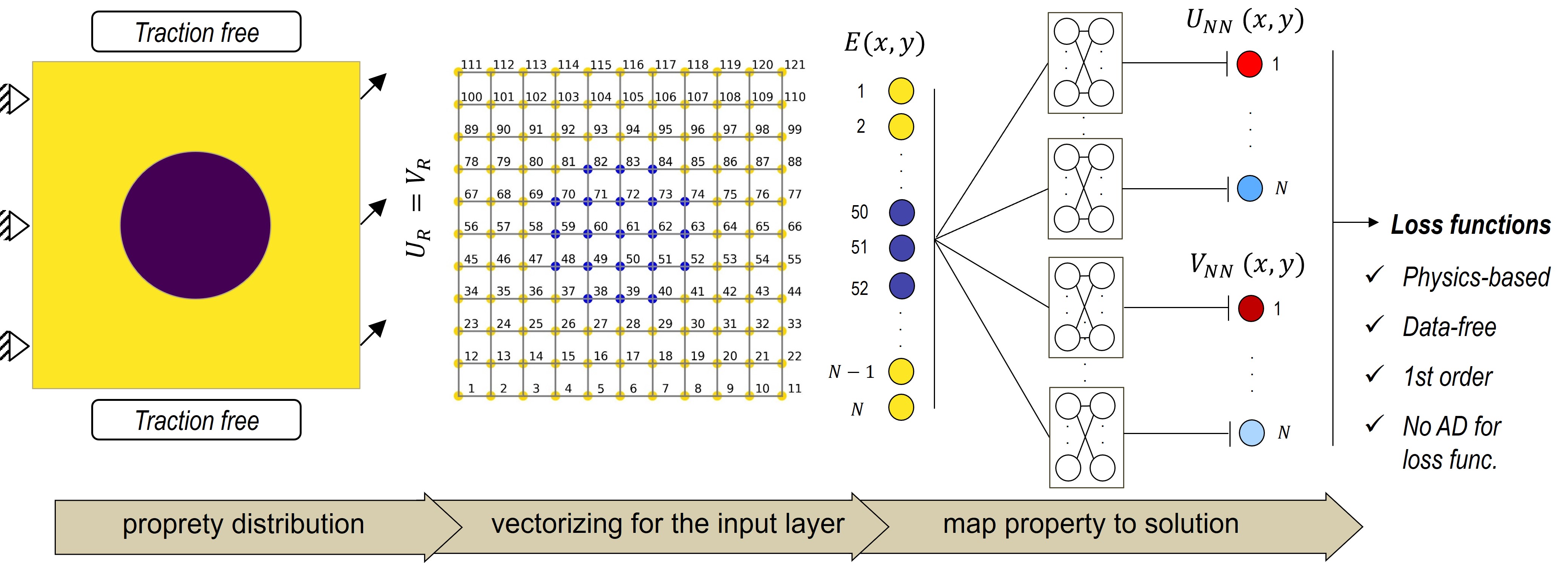
Figure 1: Network architecture for finite operator learning (FOL), where information about the Young modulus distribution goes in and the unknown displacement components are evaluated utilizing a series of separate deep neural networks. For constructing the physical loss function, automatic differentiation (AD) is not required.

Note that in Fig. 1 and throughout the rest of the work, we assume that the Poisson ratio remains constant in the domain, and our focus lies solely on the variation of Young’s modulus. The latter assumption helps to simplify the input parameter space but does not constrain the methodology. Furthermore, the stress and strain components can be derived from the predicted values of deformation in the $x$ and $y$ directions. Moreover, by increasing the number of nodes ($N$), the number of sub-networks will also increase to automatically adapt the neural network for the new parametric input space. Next, we introduce the loss function. We assume traction-free boundary conditions on the top and bottom edges, resulting in vanishing traction at the Neumann boundaries. The displacement components at the left edge are fixed (i.e., $\bar{U}=\bar{V}=0$). On the right edge, we apply tension and shear simultaneously (i.e., $\bar{U}=\bar{V}=0.05~{}$mm on Fig. 1.) leading to a rather general Dirichlet boundary condition.

The total loss term $\mathcal{L}_{\text{tot}}$ combines both the elemental energy form of the governing equation $\mathcal{L}_{\text{en,e}}$ and the Dirichlet boundary terms $\mathcal{L}_{\text{db,i}}$. It is important to note that, thanks to the weak formulation, the Neumann boundary conditions are automatically included in $\mathcal{L}_{\text{en,e}}$. Following the approach outlined in [50] for thermal problems, the total loss function involves the integration of element residual vectors (i.e., Eq. 16) using Gaussian integration, resulting in

$$\mathcal{L}_{tot} =\sum_{e=1}^{n_{el}}\mathcal{L}_{en,e}(\boldsymbol{\theta})+\sum_{i=1}^{n_{db}}\mathcal{L}_{db,i}(\boldsymbol{\theta}),$$ (20)

$$\mathcal{L}_{en,e} =\boldsymbol{U}^{T}_{e}(\boldsymbol{\theta})\left[\boldsymbol{K}_{e}~{}\boldsymbol{U}_{e}(\boldsymbol{\theta})\right],$$ (21)

$$\mathcal{L}_{db,i} =\dfrac{1}{n_{db}}|U_{i}(\boldsymbol{\theta})-U_{i,db}|+\dfrac{1}{n_{db}}|V_{i}(\boldsymbol{\theta})-V_{i,db}|,$$ (22)

$$\boldsymbol{K}_{e} =\sum_{n=1}^{n_{int}}\dfrac{w_{n}}{2}~{}\text{det}(\boldsymbol{J})~{}[\boldsymbol{B}(\boldsymbol{\xi}_{n})]^{T}\boldsymbol{C}_{e}(\boldsymbol{\xi}_{n})\boldsymbol{B}(\boldsymbol{\xi}_{n}),$$ (23)

$$\boldsymbol{C}_{e}(\boldsymbol{\xi}_{n}) =\dfrac{\boldsymbol{N}(\boldsymbol{\xi}_{n})\boldsymbol{E}_{e}}{1-\nu^{2}}\,\begin{bmatrix}1&\nu&0\\ \nu&1&0\\ 0&0&\dfrac{1-\nu}{2}\end{bmatrix}.$$ (24)

Here, $n_{\text{int}}=4$ represents the number of Gaussian integration points. Additionally, $\boldsymbol{\xi}_{n}$ and $w_{n}$ denote the coordinates and weighting of the $n$-th integration point and the determinant of the Jacobian matrix is denoted by $\text{det}(\boldsymbol{J})$. See also Appendix A. In Eq. 22, $n_{\text{db}}=22$ denotes the number of nodes along the Dirichlet boundaries (i.e., the left and right edges). Additionally, $U_{i,\text{db}}$ and $V_{i,\text{db}}$ represent the given displacement at node $i$. The final loss function reads

$$\boxed{\mathcal{L}_{tot}=a_{e}\sum_{e=1}^{n_{el}}\boldsymbol{U}^{T}_{e}\left[\boldsymbol{\sum}_{n=1}^{n_{int}}~{}\boldsymbol{B}^{T}\boldsymbol{C}_{e}\boldsymbol{B}\right]\boldsymbol{U}_{e}+a_{b}\sum_{i=1}^{n_{db}}|U_{i}-U_{i,db}|+|V_{i}-V_{i,db}|}.$$ (25)

In the above relation, the determinant of the Jacobian matrix is constant since we use quadrilateral elements. Additionally, in the four integration points we specify weightings $w_{n}=1$ and $a_{e}=\dfrac{w_{n}}{2}\text{det}(\boldsymbol{J})$ and $a_{b}=\dfrac{A}{n_{\text{db}}}$. Furthermore, in Eq. 25, $a_{b}$ represents the weighting of the boundary terms which guarantees the enforcement of the boundary conditions. Note that in Eq. 25, we utilized the discretized energy form, but one can also use the norm of the total residual vector. The total loss term $\mathcal{L}_{tot}$ is minimized with respect to the network parameters $\bm{\theta}$ concerning a batch of collocation fields.

3.2 Short review on the DeepONet model

Building on the foundational principles of the universal approximation theorem [51], the so-called vanilla DeepONet architecture [8] with two outputs is used here. The network architecture consists of a single branch and single trunk network as depicted in Fig. 2.

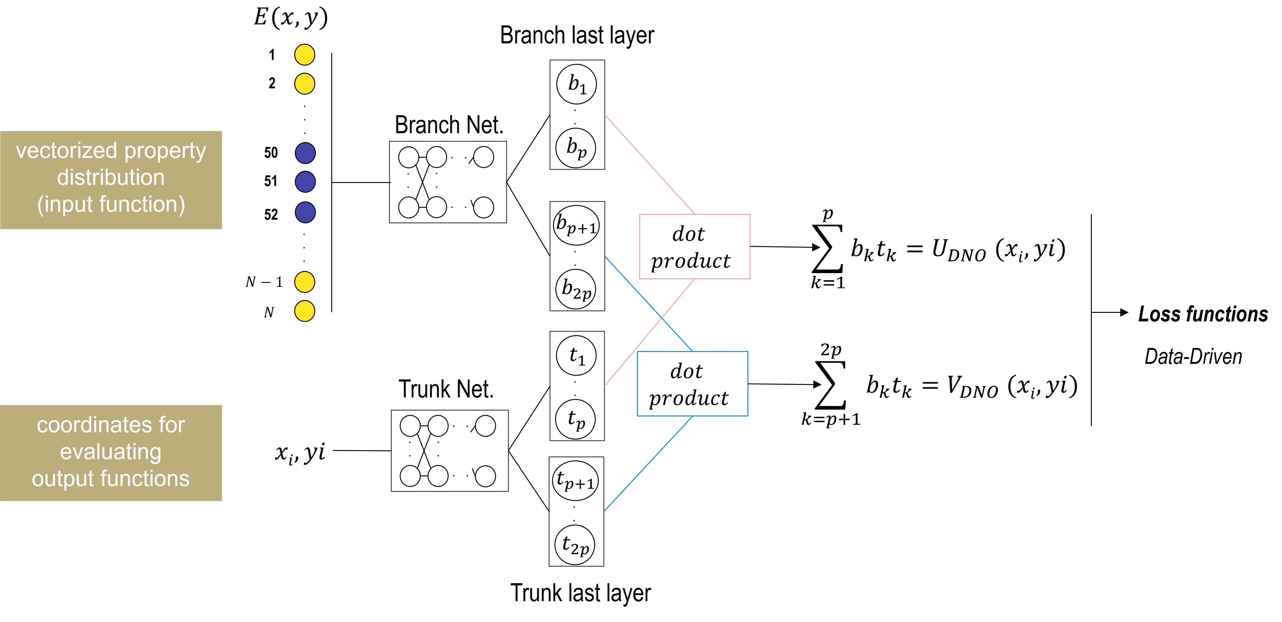
Figure 2: DeepONet’s architecture for translating property maps into mechanical deformations. The property map is vectorized and sampled at nodes (acting as sensors) to serve as input to the branch network, while the trunk network receives coordinates for output evaluation. Both networks may have different hidden layers, but end up with the same number of neurons in their final layers, which are divided into two equal-length vectors. The dot product of these vectors produces the desired outputs ($U_{i}$ and $V_{i}$).

To obtain multiple outputs from a single DeepONet, we divide the final layers of the branch and trunk networks into two parts of equal length (see also [52]). Two operators that map the property distribution to the mechanical deformations are written as

$$\mathbf{G}_{\bm{\theta}}^{(U)}(\bm{E})(\bm{X}) =\sum_{k=1}^{p}b_{k}\left(E(x_{1},y_{1}),E(x_{2},y_{2}),\ldots,E(x_{N},y_{N})\right)\cdot t_{k}(\bm{X}),$$ (26)

$$\mathbf{G}_{\bm{\theta}}^{(V)}(\bm{E})(\bm{X}) =\sum_{k=p+1}^{2p}b_{k}\left(E(x_{1},y_{1}),E(x_{2},y_{2}),\ldots,E(x_{N},y_{N})\right)\cdot t_{k}(\bm{X}).$$

In Eq.,26, $\mathbf{G}^{(U)}$ and $\mathbf{G}^{(V)}$ denote the solution operators for displacements in the $x$ and $y$ directions, respectively. Finally, for the pure data-driven DeepONet, the total loss function is written as

$$\mathcal{L}_{DeepONet}\, =\dfrac{1}{I_{train}\,N}\,\sum_{i=1}^{I_{train}}\,\sum_{j=1}^{N}|\mathbf{G}_{\bm{\theta}}^{(U)}(\bm{E}^{(i)})(\bm{X}_{j}^{(i)})-U^{(i)}_{j}|^{2}\,+\,|\mathbf{G}_{\bm{\theta}}^{(V)}(\bm{E}^{(i)})(\bm{X}_{j}^{(i)})-V^{(i)}_{j}|^{2}.$$ (27)

For more details about the DeepONet training see Appendix B. It’s worth noting that several enhancements have been introduced to improve the performance of the original DeepONet architecture [52, 53].

3.3 Preparation of collocation fields

The neural network mentioned above should be trained using initial input samples representing the Young modulus distribution. It is important to note that the training process is entirely unsupervised (i.e. no FE solution is required) and random fields are sufficient to initiate the training by having the loss function based on discretized FEM residual vector.

In the current work, we consider two-phase heterogeneous materials, which is a common example in many alloys and composite materials [54, 55]. The goal is to modify the microstructure’s morphology and properties, allowing for arbitrary shapes and volume fraction ratios between the two phases. However, the elastic properties (i.e., Young’s modulus and Poisson ratio) of each phase remain fixed. Additionally, to reduce complexity, we shall investigate at first only one ratio between the elastic properties of each phase.

So far, we have the following model simplifications: keeping the Poisson ratio and phase contrast ratio constant, and using a grid of 11 by 11. Even with the previously mentioned simplifications, there can be approximately $2^{121}\approx 2.6\times 10^{36}$ independent samples. Creating all these samples is unfeasible and may be unnecessary depending on considered application. Hence, the user should determine the relevant parameter space, specific to each problem, thereby preventing unnecessary complications. The latter point can be a challenging aspect in designing a very general deep learning model that works for all cases.

As mentioned, our preliminary motivation relies on two-phase metallic materials, and after some investigations, we have created simply a rather meaningful set of samples for training. Readers are referred to [50], for further explanations on creating these morphologies. We generated $4000$ samples for a grid of size $\sqrt{N}$ by $\sqrt{N}$, with $\sqrt{N}=11$. On Fig. 3, where the generated microstructures are sorted based on their phase fraction value, six samples with low and high phase fraction values are shown.

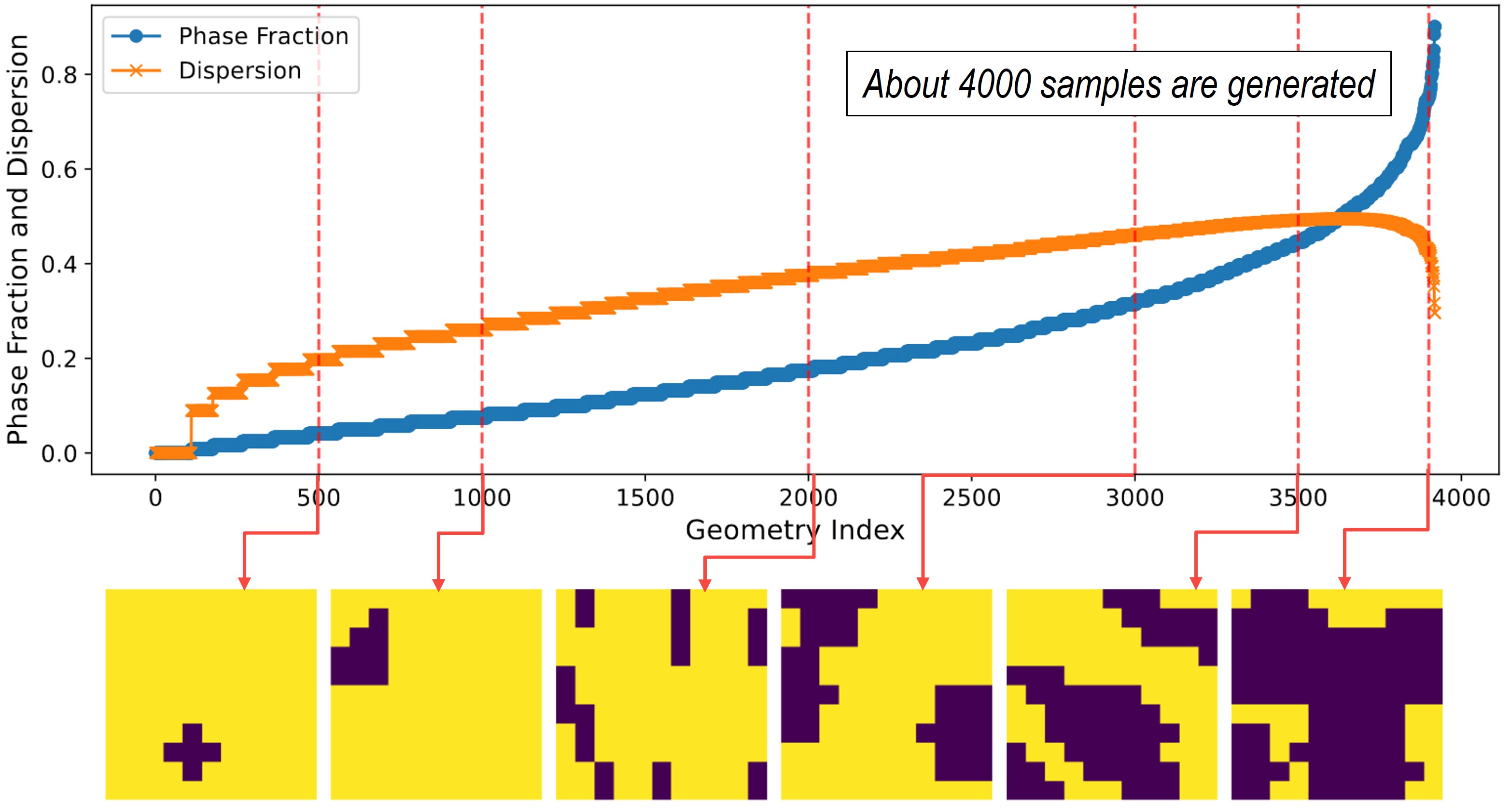
Figure 3: Examples showcasing created morphologies for a two-phase microstructure.

Additionally, to assess the NN’s performance, additional samples are chosen for testing, five of them are shown in Fig. 4. These samples are entirely novel and deliberately selected for their symmetrical aspects, ensuring they are beyond the scope of the training dataset. These samples are also motivated by dual-phase architectures in composite materials, where a soft and hard phase are combined to tune the desired effective elastic properties of the material on the macroscale. Note that all the samples are downsized to be represented by an 11 by 11 grid (i.e., 10 finite elements in each direction). The downsampling strategy is also described in [50], where a simple CNN algorithm combined with a max-pooling is used [56]. See also Fig. 5 for relative histograms of the created samples. Note that we consider a rather unsymmetrical distribution to examine the interpolation capabilities of the trained model.

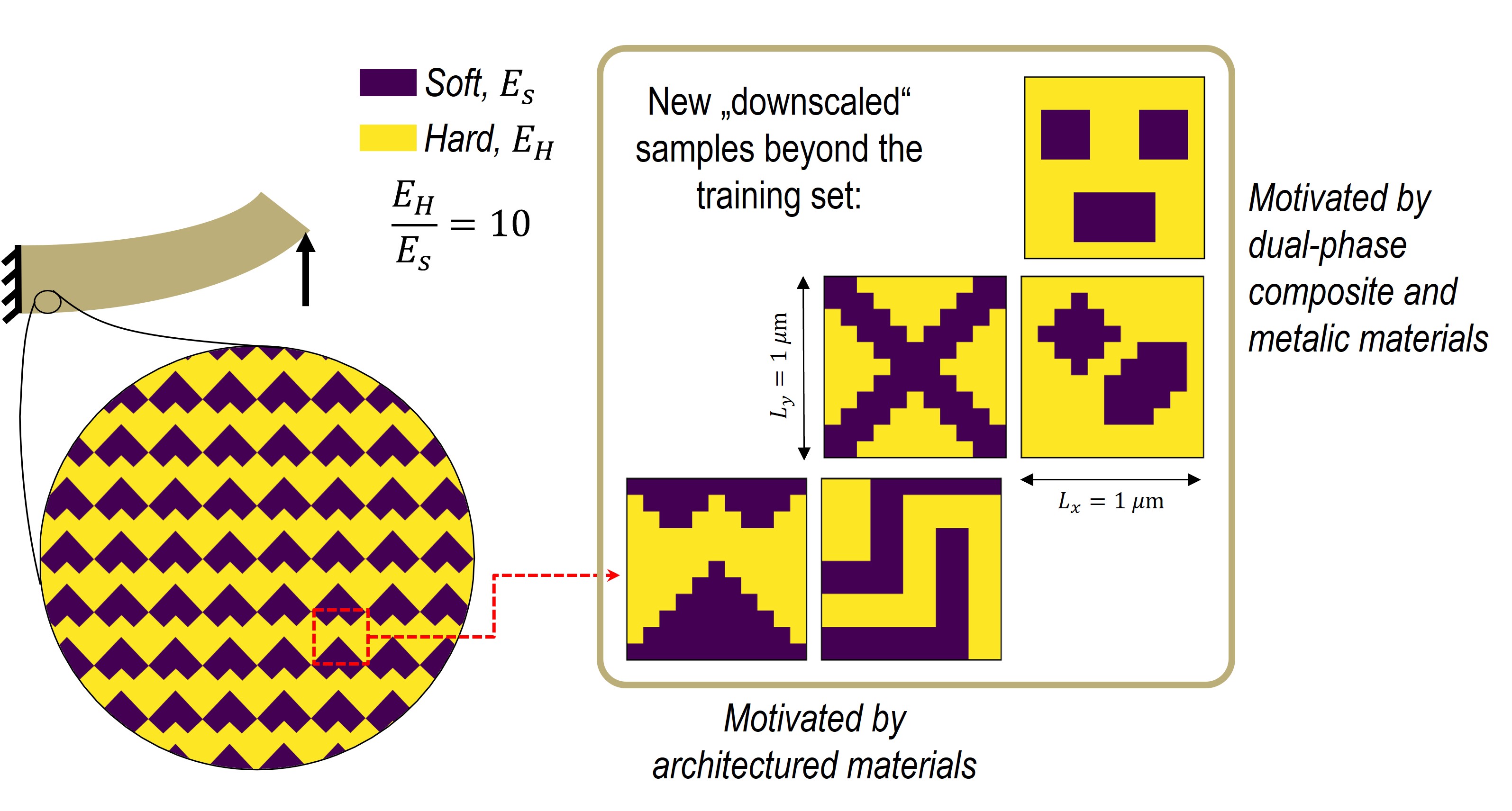
Figure 4: Unseen samples used for testing the neural network after training.

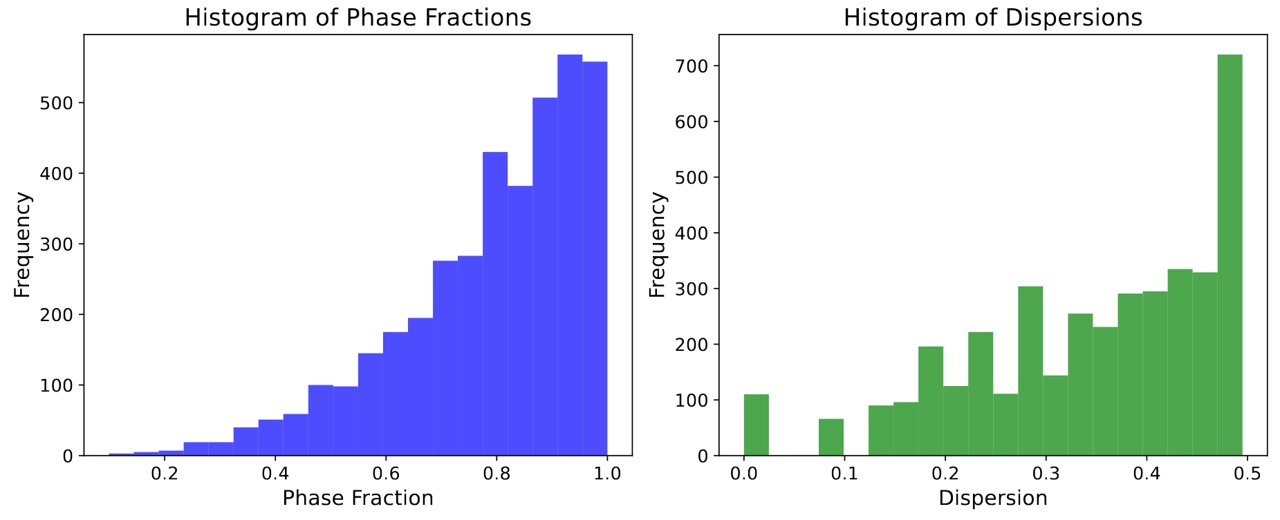
Figure 5: Histogram of the phase fraction as well as dispersion values of the created samples.

4 Results

The algorithms developed in this study are implemented using the SciANN package [57], and the methodology can be adapted to other programming platforms. A summary of the network’s (hyper)parameters is presented in Table 1. Note that whenever multiple options for a parameter are introduced, we examine the influence of each parameter on the results. Training was mainly done on personal laptops without relying on GPU acceleration, as the computations were not computationally intensive here.

Table 1: Summary of the network parameters.

Parameter	Value
Inputs, Outputs	$\{E_{j}\}=\{E_{1},\cdots,E_{N}\},~{}[\{U_{i}\}=\{U_{1},\cdots,U_{N}\},~{}\{V_{i}\}=\{V_{1},\cdots,V_{N}\}]$
Activation function	Swish [58]
Layers and neurons for each sub-network	$(L,N_{l})=(2,10)$
Optimizer	Adam [59]
(Number of samples, Batch size)	$(100,2)$, $(1000,25)$, $(2000,50)$, $(4000,100)$
(Learning rate $\alpha$, Number of epochs)	$(5\times 10^{-4},4000)$

The material parameters listed in Table 2 do not necessarily represent a specific material at this point. For the chosen Young modulus values and boundary conditions we did not see the necessity to perform any additional normalization before the training.

Table 2: Model input parameters for the mechanical problem.

	Young modulus value/unit
Phase 1 ($E_{H}$)	$1.0$ MPa
Phase 2 ($E_{S}$)	$0.1$ MPa
Applied displacement, small defo. model ($U_{R}$,$V_{R}$)	($0.05$ mm, $0.05$ mm)

4.1 Evolution of loss function and network prediction

The evolution of each loss term is illustrated in Fig. 6 throughout epochs. On the left-hand side, the loss terms associated with the physics-driven model are presented, while the right-hand side displays the loss evolution for the supervised data-driven model. It is noteworthy that satisfactory results are achieved only after $4000$ epochs in both cases. It is important to mention that, for the data-driven model, offline finite element calculations are performed on the same set of 4000 samples, and the identical network architecture is employed as in the physics-driven model.

In Fig. 6, we employ the ”swish” activation function, and 4000 samples with a batch size of 100 are used for training while the remaining parameters align with those in Table 1. All the loss functions decay simultaneously, and we did not observe any significant improvement after $4000$ epochs. Further comparisons regarding the training and evaluation costs are detailed in Table 3.

For the loss term related to the Dirichlet boundary conditions, we assigned higher weightings to satisfy the boundary terms. Following a systematic study that began with equal weightings for both loss terms, we selected $A=10~{}n_{nb}$, indicating $a_{b}=10$. Choosing equal or lower weightings resulted in less accurate predictions within the same number of epochs, as the boundary terms were not fully satisfied. Opting for higher values did not significantly improve the results. It is worth mentioning that with the current approach, one can also easily apply hard boundary constraints by omitting nodes (i.e., degrees of freedom) with Dirichlet boundary conditions from the output layers. We intentionally did not perform this for the current study to demonstrate that even with simple soft constraints, one can train the neural network properly. This aspect is crucial for extending the neural network to learn different boundary conditions in a parametric way for future work.

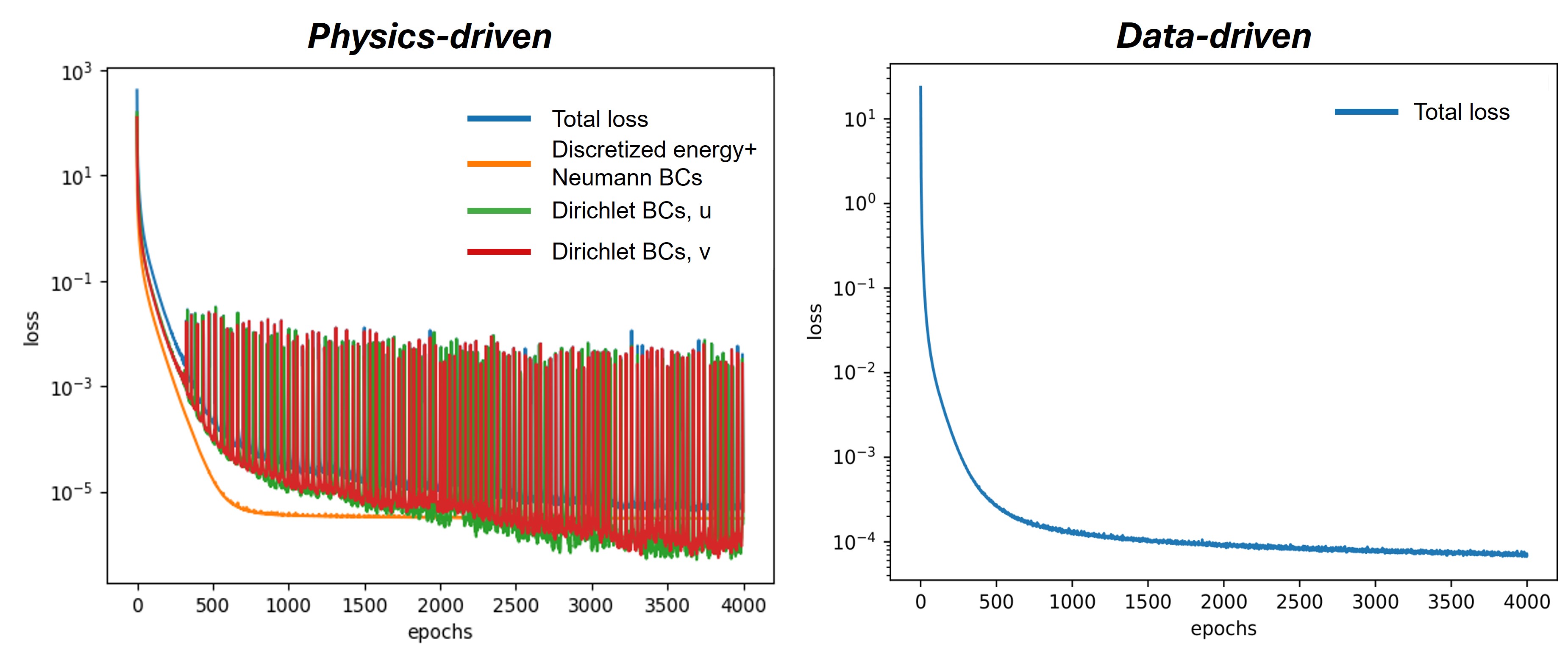
Figure 6: Evolution of loss terms for parametric learning of the quasi-static mechanical equilibrium problem.

In Figures 7 to 9, the predictions of the same neural network for various microstructures are depicted. In the middle part of the figures, we display the reference solutions obtained by the FEM, utilizing the same number of linear elements ($10$ by $10$). Note that post-training, the results are assessed on finer meshes ($100\times 100$) using bi-linear shape function interpolations. See also discussions in the next section for further details. On the right-hand side, the absolute value of the point-wise difference between FOL and FEM is shown. All displacement values are denoted in micrometer $[\mu$m], stress components are represented in [GPa], and Young modulus is expressed in [GPa] too.

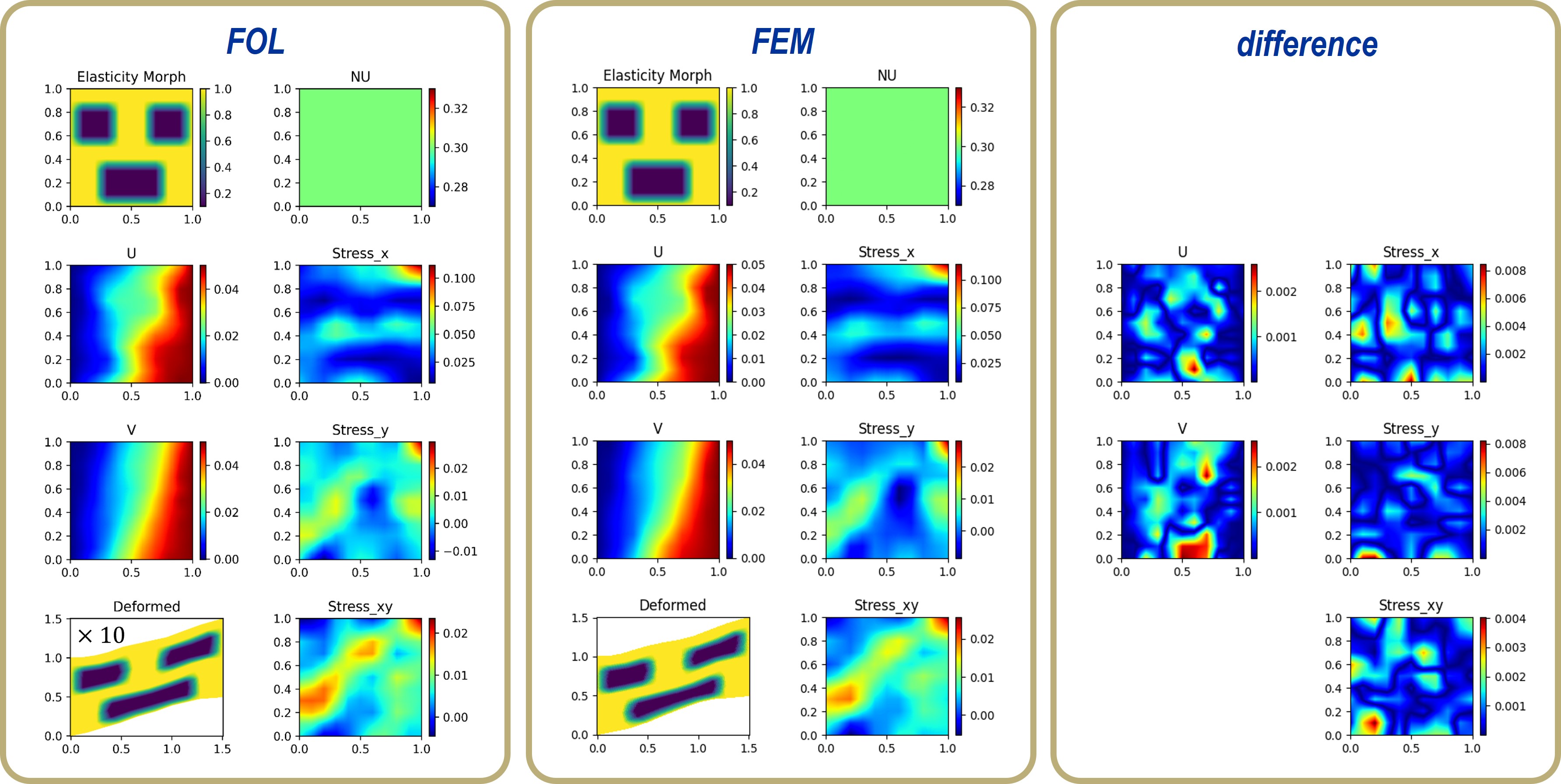
Figure 7: Predictions of the trained FOL for a test case with three square shape inclusions.

The predictions of the neural network for unseen microstructures are in very good agreement with those from the FEM. The maximum pointwise error for displacement components remains below $10\%$, localized only in some points of the entire domain. For the stress components, which are obtained through post-processing of deformations values, the errors are higher, as expected, since the neural network predictions are solely based on deformations, and any higher-order derivatives are more sensitive to slight deviations in the original solution. On the other hand, for many applications in multiscale material modeling, homogenized values of stress and strain components are needed, and these are well-predicted as outlined in Section 4.2.

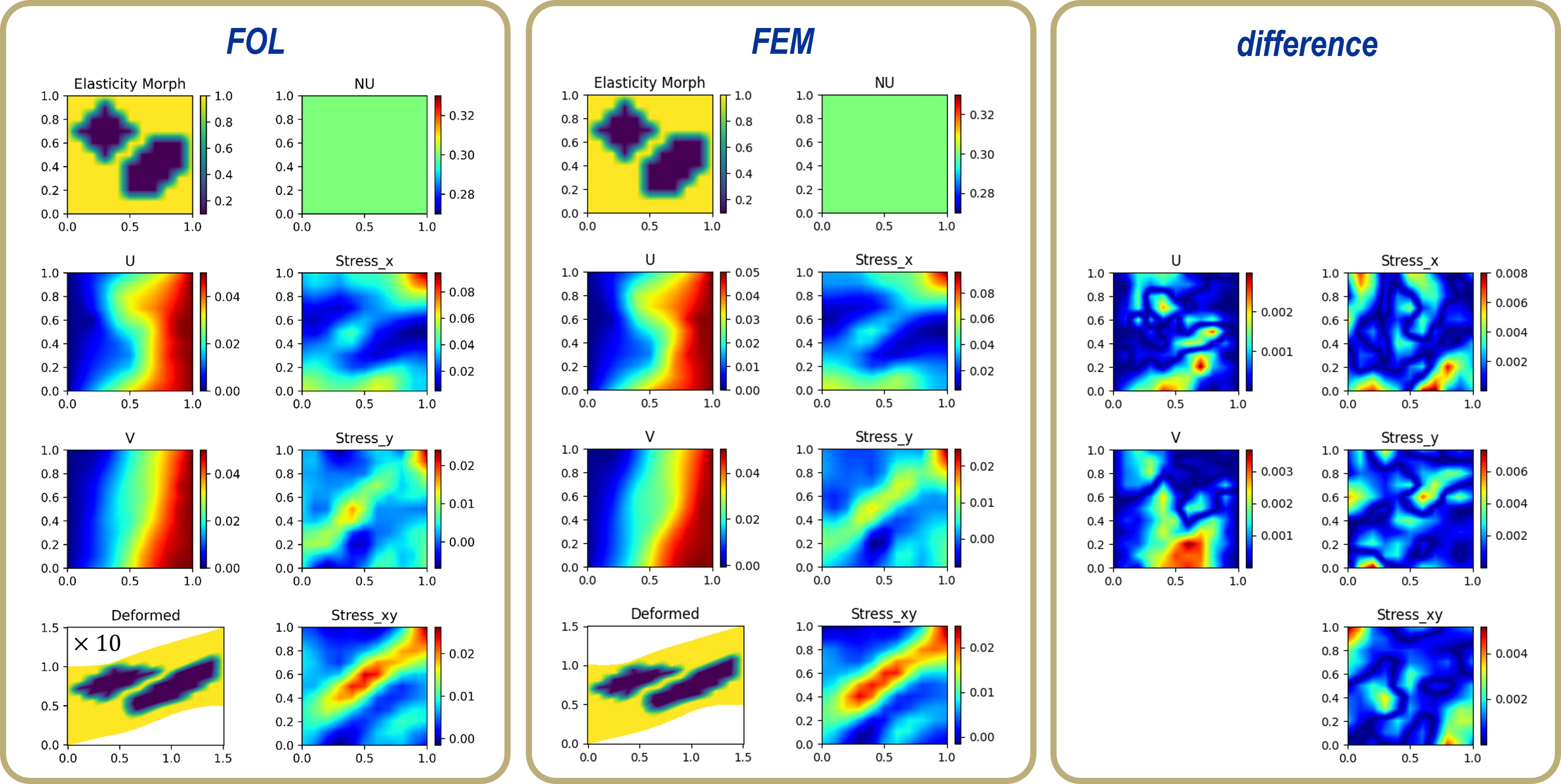
Figure 8: Predictions of the trained FOL for approximately circular and ellipsoidal inclusions.

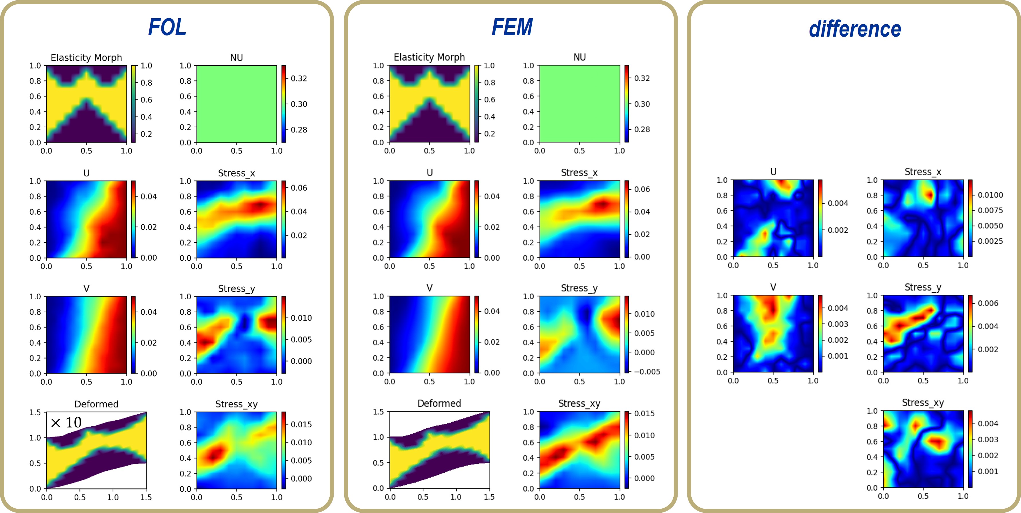
Figure 9: Predictions of the trained FOL for test similar to architectured materials which behave anisotropic.

4.2 Discussions on up-scaling results and mesh convergence

To minimize training costs, the microstructure morphologies (i.e., Young modulus distributions) undergo downsampling onto a smaller grid. The question arises regarding potential information loss and methods to reconstruct the original solution. In Fig. 10, various approaches are demonstrated for this purpose. The first method involves linear interpolation of the solution in the domain, proving to be both cost-effective and implementable, resulting in an acceptable agreement between the original and upsampled solutions (see the right-hand side of Fig. 11). This success motivates its further use in the current study. Quadratic interpolation is also explored, but despite its smoothness, it does not provide significant advantages. Certainly, the most effective yet more costly strategy involves utilizing a pre-trained decoder, as shown on the right-hand side of Fig.10. Training such a decoder requires solution data and additional training efforts and will be investigated in the near future.

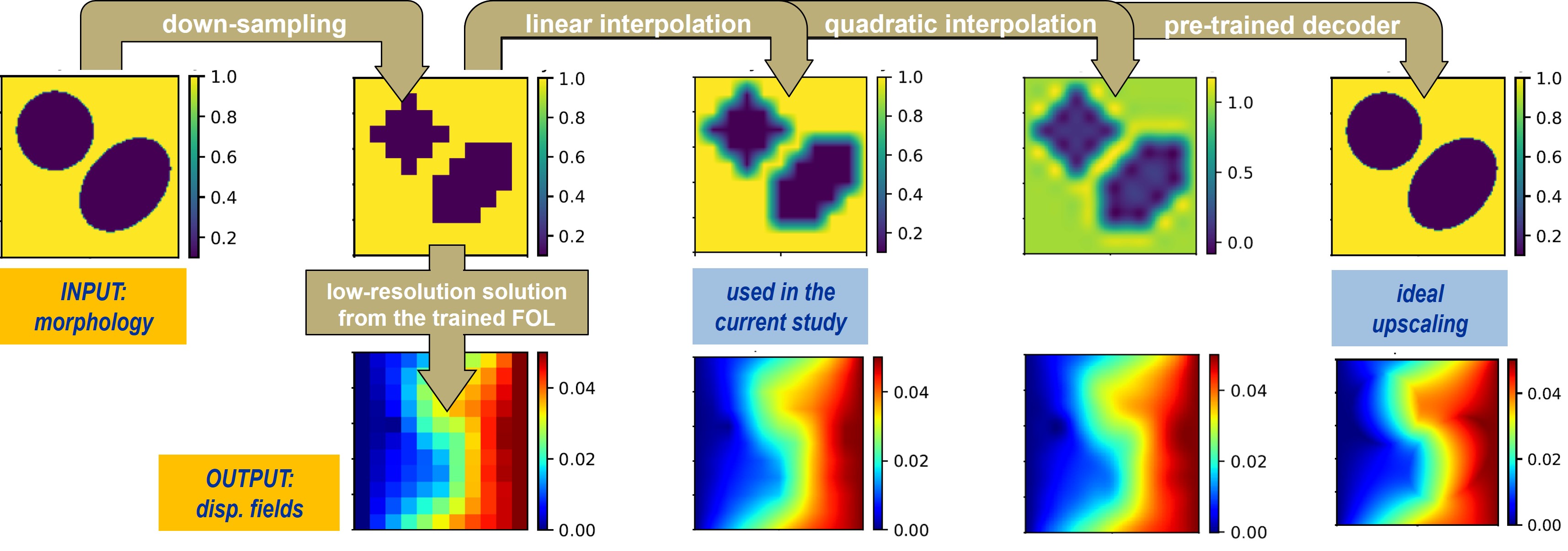
Figure 10: Different strategies for upsampling the results (displacement component $U$).

In Fig. 11, we demonstrate the convergence of the FE solution as the mesh size is refined. We observe that the upscaled results continue to align closely with the reference solution (with about $10\%$ difference localized near the phase boundaries), showcasing excellent efficiency in terms of normalized computational cost $T$.

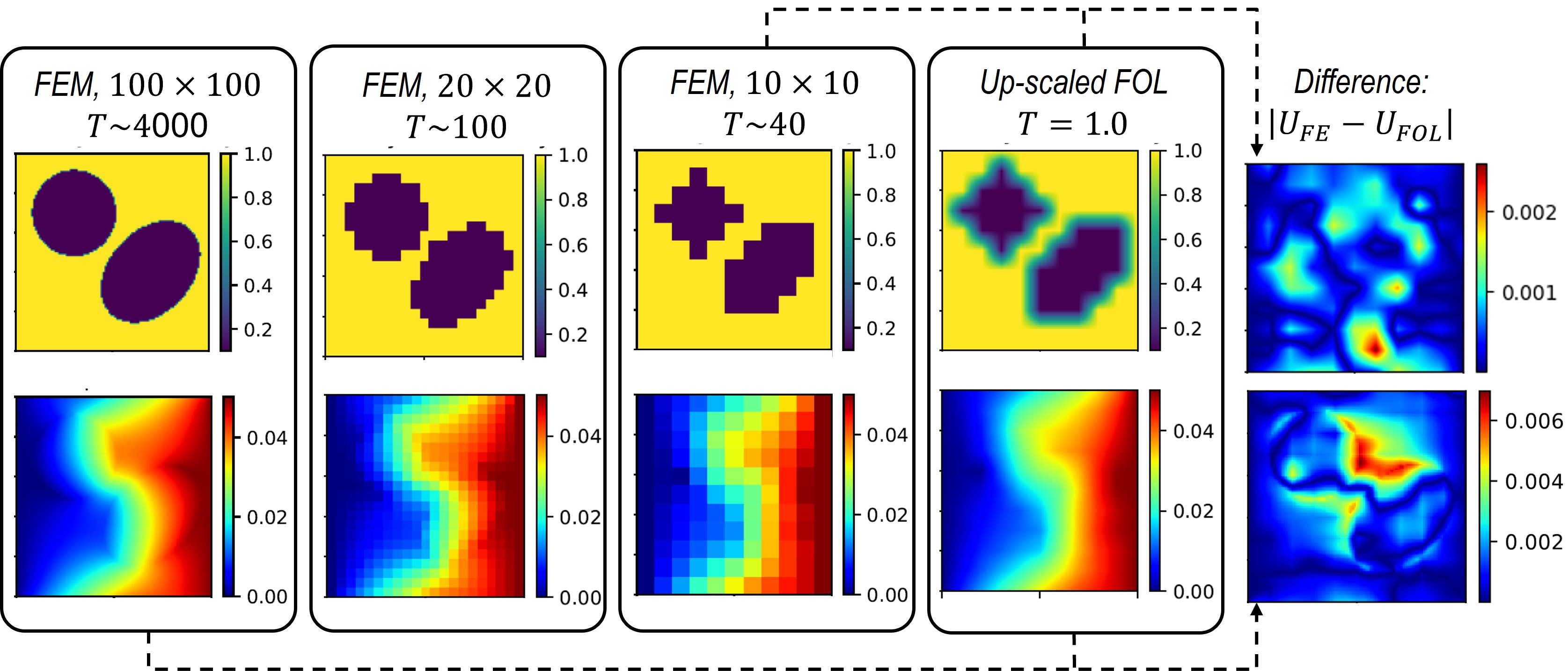
Figure 11: Convergence of the FE results for the displacement component $U$ and comparison of the upscaled FOL with the FE solution.

4.3 Comparison of physics-driven and data-driven deep learning models

This section’s objective is to highlight the advantages of using physical laws to train networks as opposed to those solely trained on data obtained from other numerical methods, such as the finite element method. For a fair comparison, we utilize the same set of $4000$ sample data, perform finite element calculations for each, and store the associated solutions. Additionally, we employ an identical network architecture to train the data-driven network. The comparison results, illustrated in Fig. 12 for several unseen test cases, reveal that the physics-driven method provides more accurate predictions for mechanical deformation as well as stress distribution. However, it’s worth noting that the performance of the current approach, trained based on data alone, is not far from the reference solutions. To show the advantages of the FOL approach other operator learning models, namely DeepONet, are investigated and trained by using the same data set (see Sec. 3.2 for details of this model). Interestingly, the results of the current approach are more accurate even with a data-driven formulation.

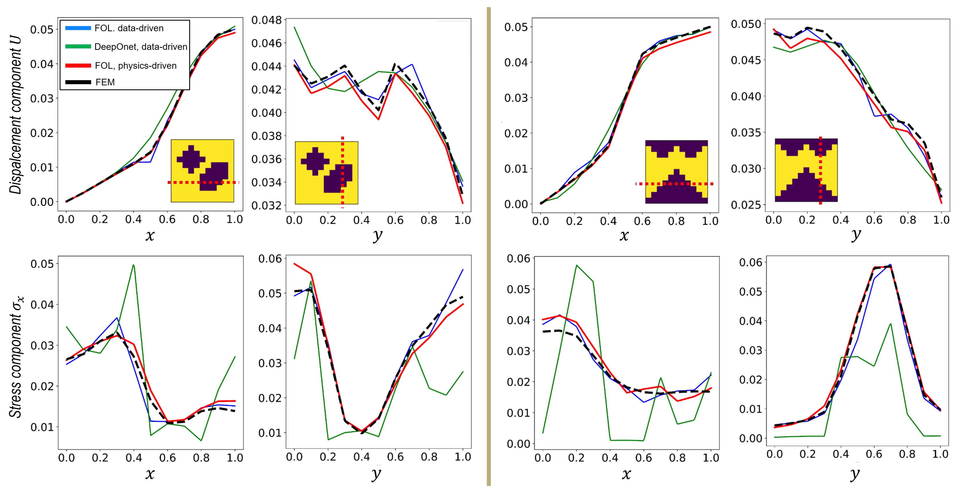
Figure 12: Comparison of data-driven FOL, data-driven DeepOnet, and physics-driven FOL approaches regarding the displacement component in x direction $U$ as well as stress component $\sigma_{x}$ along $x$ and $y$ directions, respectively.

This highlights the attractiveness of the physics-driven FOL for two main reasons: Firstly, it operates without the need for labeled data during training, and secondly, it provides more accurate predictions for unseen cases for both displacement components (as primary variables) and their spatial derivatives (i.e., stress components). Nevertheless, it is essential to emphasize that supervised training incurs a lower training cost, averaging approximately $7$ to $10$ times less compared to the physics-based approach. The observations discussed above are not limited to a specific test case or the selected cross sections; they consistently appear across other unseen cases and regions as well.

It is noteworthy that in future works, other operator learning approaches should be properly compared under the same data/sample set to enable a fair comparison.

4.4 The effect of the number of initial samples

In Figs. 13 and 14, we not only compare the performance of the data-driven and physics-driven FOL models but also study the influence of the initial training samples on the final predictions. Note that other (hyper)parameters of the NNs are kept the same for this study (e.g., the same number of epochs, learning rate, and activation function are used as the previous network’s architecture). See also Tab. 1 for the chosen batch sizes for each case. As expected, reducing the number of samples from the initial dataset leads to increased errors. In other words, by training with more samples with proper distribution and variety, the deep learning model has the chance to map much better between two parametric spaces.

What is noteworthy from such observations is how accurately the physics-driven model can predict the solution even when trained based on $2000$ initial random samples. This confirms that providing equations for training has a more significant impact on the network performance and learning procedure. To confirm this observation, we tested several cases with different complexities in the next section.

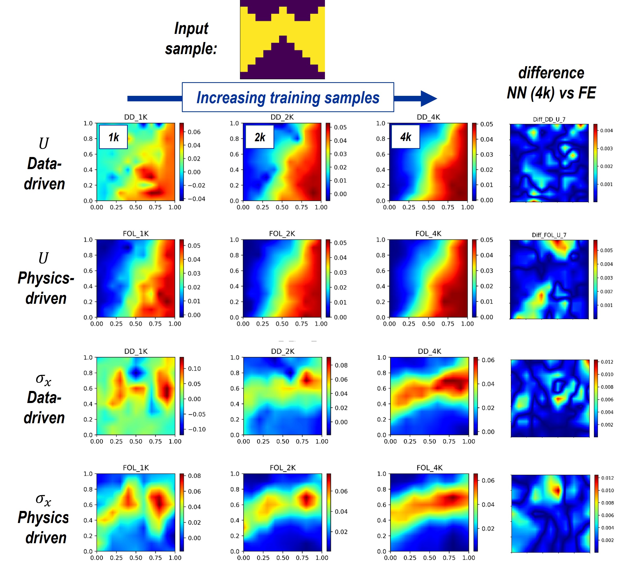
Figure 13: Performance of data-driven and physics-driven approaches for different number of training samples.

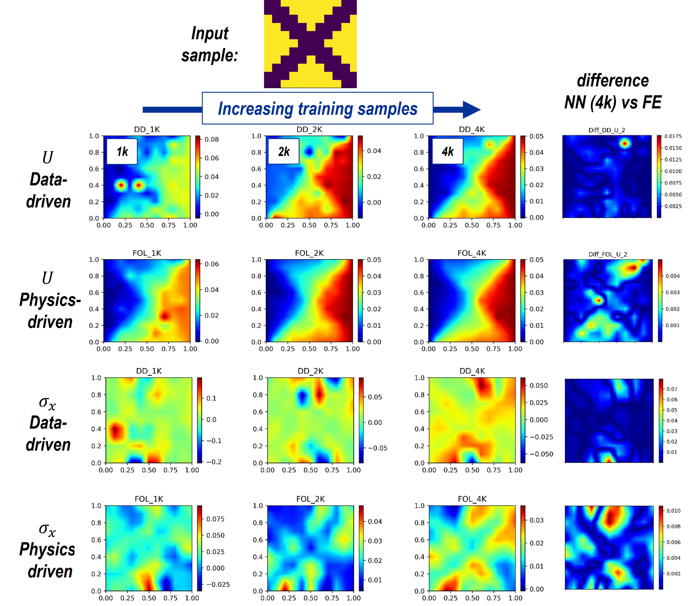
Figure 14: Performance of data-driven and physics-driven approaches for different number of training samples.

In Fig. 15, we present quantitative error measurements by using different error metrics for four distinct unseen test cases. Error metrics are defined as: $Err_{MSE}=\sqrt{\frac{1}{N}\sum_{i}(u_{NN}(i)-u_{FE}(i))^{2}}$ or as $Err_{MAX}=\text{Max}(|u_{NN}(i)-u_{FE}(i)|)$. The former indicates the average pointwise error, while the latter focuses on the maximum local difference. Training the model with more samples enhances its performance, and one can observe a convergence behavior similar to that of other numerical methods, despite being based on a different concept here.

From the comparison of error plots, two interesting points emerge. Firstly, the errors for the physics-driven model are generally lower than those for the data-driven model, regardless of the number of sample fields used for training the model (compare the solid to the dashed line with the same color). Secondly, for test case 1, which is more similar to the samples used for training, the errors of the data-driven model are very acceptable. This indicates that, apart from the quantity of the samples, the so-called quality of them plays a role. In other words, even if it sounds rather unfeasible to train the model for any possible distribution of Young modulus, one can always select a meaningful set of samples for each specific application to train the model properly.

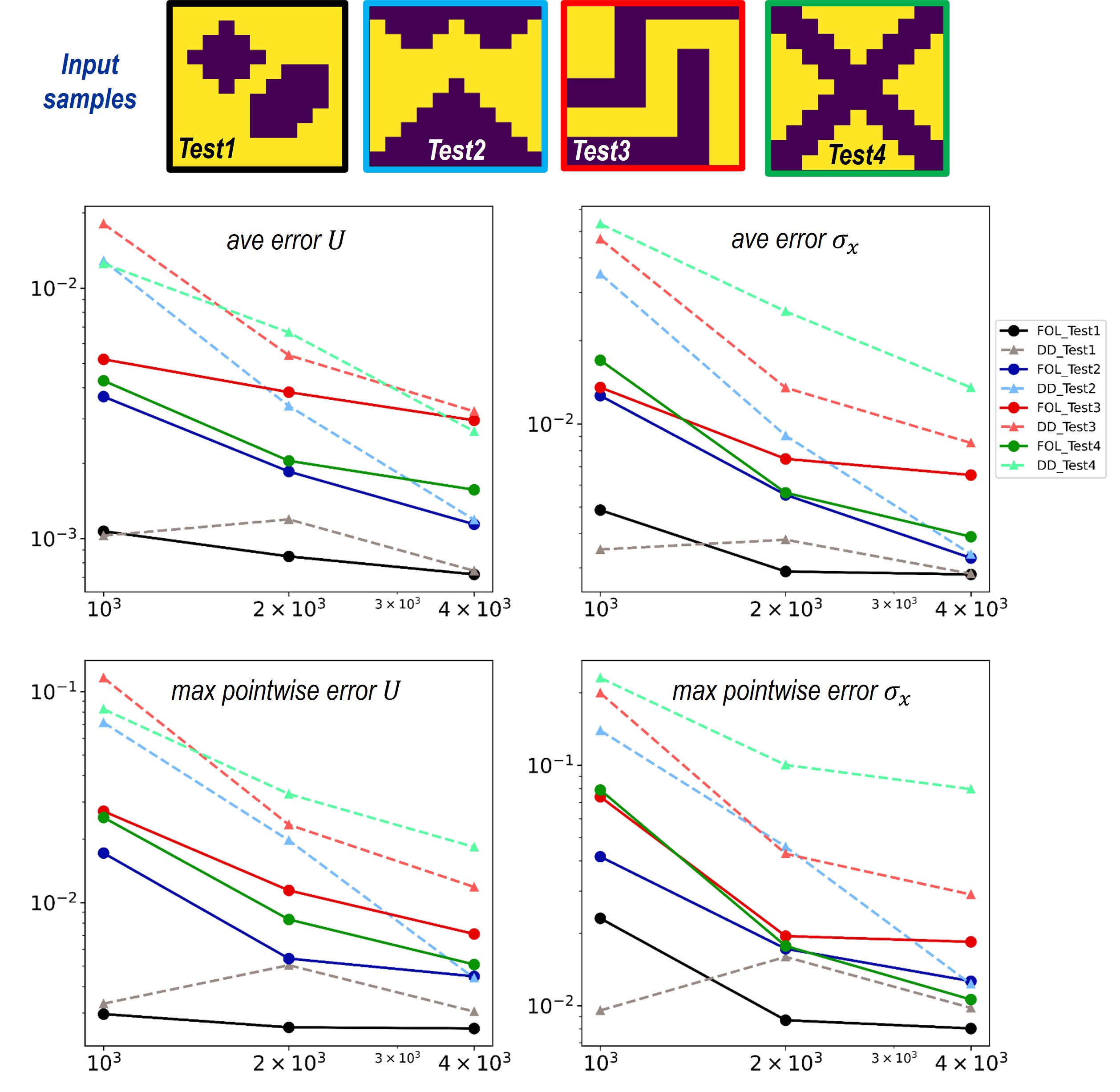
Figure 15: Improving the performance of the deep learning models by increasing the number of randomly generated samples for training. Different error evaluations are utilized based on different applications, where the physics-driven model always behaves better than the data-driven one for the same unseen test cases.

For test cases 3 and 4, we observe higher errors with both error metrics, as they are significantly distant from the sample shapes considered during training. Therefore, we expect that by further enriching the initial sample fields, the errors for these two cases will decrease. It is important to emphasize that, although we explored various sensitivities and hyperparameters, the training of both the data-driven and physics-driven models in this study could potentially be enhanced in future studies by considering other optimizers or exploring ideas from Taylor or Fourier features, which are not covered in this study.

4.5 Influence of phase contrast on the results

In this section, we briefly discuss the changes in the phase contrast (ratio of the Young modulus) based on the obtained results from the FOL. So far, we mainly focused on the ratio of $E_{H}/E_{S}=10$. In Fig. 16, we also showed the averaged error for the displacement component $U$ in the $x$ direction as we increase and decrease the stiffness ratio to $E_{H}/E_{S}=20$. These latter values are roughly representative of some engineering applications in composite and dual-phase metallic materials.

We can conclude that by increasing the ratio, the errors generally tend to slightly increase. This is attributable to the anticipation of higher jumps and greater nonlinearities and complexities in the deformation profiles. Also, note that the morphology of unit cell 2 presents more interfaces between both phases than unit cell 1, which can be another reason for higher errors. One potential solution for addressing this issue could involve the integration of a mixed formulation [20] into the current framework or training based on a larger number of initial samples for higher epochs.

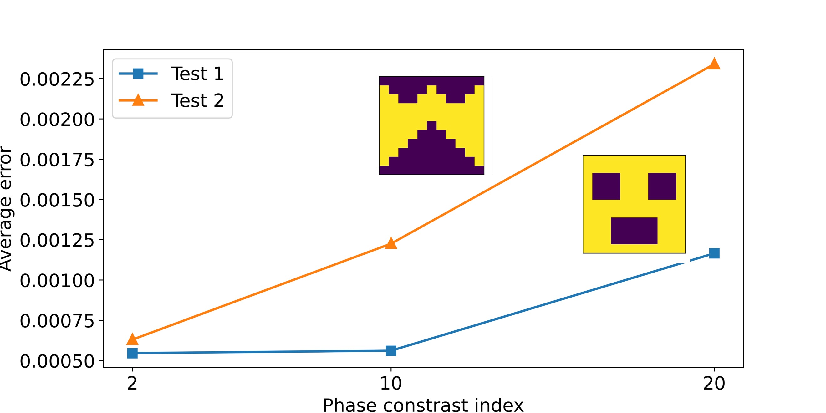
Figure 16: Influence of ratio of phase contrast on the obtained results.

4.6 Discussions on computational cost

Due to its concise formulation employing elementwise domain decomposition from the finite element discretization and leveraging shape functions, the introduced method for physics-based operator learning enables an exceptionally efficient model training process. Tab. 3 illustrates the required training time per epoch for the discussed mechanical problem. Employing a standard Adam optimizer for approximately $4000$ epochs yields satisfactory results. When training the same architecture based on data, the time investment is lower, as highlighted in Tab. 3. Once the model is trained, evaluating the neural network becomes remarkably economical for any arbitrary input parameter which is about 20 times faster than the standard FEM.

Table 3: Comparison of the computational costs per epoch.

-	norm. ave. run-time
Training FOL (physics-driven) with $4000$ samples, batch size = 100	$1.0$
Training FOL (data-driven) with 4000 samples, batch size = 100	$0.15$
Network evaluation after training (data or physics driven)	$1.0$
Finite element calculation ($11\times 11$ grid)	$40$
Finite element calculation ($101\times 101$ grid)	$4000$

5 Conclusion and outlooks

This work presents a data-free, physics-based method for parametric learning of partial differential equations in mechanics of heterogeneous materials. This method relies solely on governing physical constraints, which are the discretized weak form of the problem as well as Dirichlet boundary terms. Leveraging the finite element method without depending on automatic differentiation for computing physical loss functions, the proposed approach approximates all derivatives using shape functions. This significantly improves training efficiency, necessitating fewer epochs and less time per epoch. Additionally, it allows flexibility in selecting activation functions without worrying about vanishing gradients. However, it’s important to mention that potential discretization errors from the finite element method persist in the present approach.

In this study, the network takes the elasticity distribution within the microstructure as input and produces the deformation components under fixed boundary conditions as output. Our method demonstrates accurate predictions of deformation fields, with the maximum pointwise error across all test cases consistently below $10\%$, primarily localized near phase boundaries. On the other hand, errors for first-order gradient terms, such as stress components, exhibit higher values. The latter observation requires further improvement in future developments, as local stress values significantly affect the localized nonlinear material behavior, such as plasticity and damage progression. On the positive side, errors for averaged or homogenized values remain around $1\%$, making them acceptable for various engineering applications as long as the material is in the elastic regime. Despite possible errors and deviations in predicting the solution, the introduced methodology offers a significant speedup of about $40$ to $50$ times over the standard finite element method in elasticity. Furthermore, compared to a data-driven approach, the introduced physics-driven method demonstrates superior accuracy for unseen input parameters.

The current investigations open up an entirely new approach for further research into combining physics-based operator learning and well-established numerical methods. Expanding this approach to nonlinear problems is essential, as it holds the potential for even greater speed improvements. While our focus was here on elastic problems in heterogeneous materials, exploring other types of equations, such as temporal problems and microstructure modeled by the phase field method presents an intriguing avenue for our future scope. Finally, it would be interesting to apply the current approach to inverse problems, wherein providing sufficient data can lead to discovering the underlying physics of the problem.

Data Availability: The codes and data associated with this research are available upon request and will be published online following the official publication of the work.

Acknowledgements: The authors would like to thank the Deutsche Forschungsgemeinschaft (DFG) for the funding support provided to develop the present work in the project Cluster of Excellence “Internet of Production” (project: 390621612). Ali Harandi and Stefanie Reese acknowledge the financial support of Transregional Collaborative Research Center SFB/TRR 339 with project number 453596084 funded by DFG gratefully.

Author Statement: S.R.: Conceptualization, Software, Writing - Review & Editing. S.F.: Supervision, Review & Editing. M.A.: Software, Writing - Review & Editing. A.H.: Software, Writing - Review & Editing. G.L.: Supervision, Review & Editing. S.R.: Supervision, Review & Editing. M.A.: Funding, Supervision, Review & Editing.

6 Appendix A: basics of finite element discretization

Here we shortly summarize the corresponding linear shape functions $\bm{N}$ and the deformation matrix $\bm{B}$ used to discretize the mechanical weak form in the current work.

$$\bm{N}=\begin{bmatrix}N_{1}&0&\dots&N_{4}&0\\ 0&N_{1}&\dots&0&N_{4}\end{bmatrix},~{}\bm{B}=\begin{bmatrix}N_{1,x}&0&\dots&N_{4,x}&0\\ 0&N_{1,y}&\dots&0&N_{4,y}\\ N_{1,y}&N_{1,x}&\dots&N_{4,y}&N_{4,x}\end{bmatrix}.$$ (28)

The notation $N_{i,x}$ and $N_{i,y}$ represent the derivatives of the shape function $N_{i}$ with respect to the coordinates $x$ and $y$, respectively. To compute these derivatives, we utilize the Jacobian matrix

$$\boldsymbol{J}=\partial\boldsymbol{X}/\partial\boldsymbol{\xi}=\begin{bmatrix}\frac{\partial x}{\partial\xi}&\frac{\partial y}{\partial\xi}\\ \frac{\partial x}{\partial\eta}&\frac{\partial y}{\partial\eta}\end{bmatrix}.$$ (29)

Here, $\boldsymbol{X}=[x,y]$ and $\boldsymbol{\xi}=[\xi,\eta]$ represent the physical and parent coordinate systems, respectively. It is worth mentioning that this determinant remains constant for parallelogram-shaped elements, eliminating the need to evaluate this term at each integration point. Readers are also encouraged to see the standard procedure in any finite element subroutine [60, 61]. Finally, for the B matrix, we have

$$\bm{B}=\bm{J}^{-1}\begin{bmatrix}\frac{\partial N_{1}}{\partial\xi}&0&\frac{\partial N_{2}}{\partial\xi}&0&\frac{\partial N_{3}}{\partial\xi}&0&\frac{\partial N_{4}}{\partial\xi}&0\\ 0&\frac{\partial N_{1}}{\partial\eta}&0&\frac{\partial N_{2}}{\partial\eta}&0&\frac{\partial N_{3}}{\partial\eta}&0&\frac{\partial N_{4}}{\partial\eta}\\ \frac{\partial N_{1}}{\partial\eta}&\frac{\partial N_{1}}{\partial\xi}&\frac{\partial N_{2}}{\partial\eta}&\frac{\partial N_{2}}{\partial\xi}&\frac{\partial N_{3}}{\partial\eta}&\frac{\partial N_{3}}{\partial\xi}&\frac{\partial N_{4}}{\partial\eta}&\frac{\partial N_{4}}{\partial\xi}\end{bmatrix}.$$ (30)

Figure 17: The physical space and the parent space. Gaussian integration and shape functions are shown specifically within the parent space.

7 Appendix B: More details on the training of the DeepONet part

In this appendix, additional details about the training process of the DeepONet network are provided. Sec. 3.2 illustrates the vanilla DeepONet network architecture in Fig.  2. The branch network processes the distribution of properties, which are measured at arbitrary sensor locations. Specifically, the input function to the branch network includes the values of Young’s modulus at the element nodes. The branch maps the input function into two distinct vectors, one for each output. They can be considered as latent vectors, see [62]. On the other hand, the trunk network is designed to receive the spatial coordinates of a single point where the output function is evaluated. Finally, two operators are built by the dot product of the last layers of the branch and the trunk.

These operators are designed to map the input function $\bm{E}$, captured at $N$ sensor locations (nodes of elements), to the corresponding solutions at the given spatial coordinate $\bm{X}=(x_{i},y_{i})$ to the trunk network.

In Eq. 27, the loss function is defined as the mean squared error (MSE) between the predicted values of the operators for $U$ and $V$ and the solutions derived using the finite element method (FEM). For each input function, indexed by $i$ and covering the entire range of training inputs up to $I_{train}$, the total number of training input functions, the operator predicts the value at each point $j$. Then the difference between these predictions and the solutions obtained by FEM over $N$ points are computed. The network parameters, denoted as $\bm{\theta}$, are then optimized by minimizing the loss function outlined in Eq. 27.

For training the network, a purely data-driven approach is employed. Details regarding the sample preparation can be found in Sec. 3.3. The training involves $4000$ samples, each featuring distinct morphology maps, and the training is done for $4000$ epochs. Since the architecture of the network differs significantly from the FOL approach, an extensive study of hyperparameters was performed to achieve optimal results. The best-performing configuration was found to be $6[20]$, which indicates $6$ hidden layers, when each layer consists of $20$ neurons. Notably, both the branch and the trunk networks use an identical architecture and share a common final layer containing $20$ neurons.

Figure 18: The decay of total loss and its $U$ and $V$ components for the DeepONet network with optimally found hyperparameters.

The best result is obtained by using the swish as the activation function. The loss decay for the optimal hyperparameters is shown in Fig. 18.

References

- Geers et al. [2010] M.G.D. Geers, V.G. Kouznetsova, and W.A.M. Brekelmans. Multi-scale computational homogenization: Trends and challenges. Journal of Computational and Applied Mathematics, 234(7):2175–2182, 2010.
- Faroughi et al. [2024] Salah A. Faroughi, Nikhil M. Pawar, Célio Fernandes, Maziar Raissi, Subasish Das, Nima K. Kalantari, and Seyed Kourosh Mahjour. Physics-Guided, Physics-Informed, and Physics-Encoded Neural Networks and Operators in Scientific Computing: Fluid and Solid Mechanics. Journal of Computing and Information Science in Engineering, 24(4):040802, 2024.
- Liu et al. [2022] Wing Kam Liu, Shaofan Li, and Harold S. Park. Eighty years of the finite element method: Birth, evolution, and future. Archives of Computational Methods in Engineering, 2022.
- Herrmann and Kollmannsberger [2024] Leon Herrmann and Stefan Kollmannsberger. Deep learning in computational mechanics: a review. Computational Mechanics, 2024.
- Kim and Lee [2024] Dongjin Kim and Jaewook Lee. A review of physics informed neural networks for multiscale analysis and inverse problems. Communications Physics, 2024.
- Lu et al. [2021] Lu Lu, Pengzhan Jin, Guofei Pang, Zhongqiang Zhang, and George Karniadakis. Learning nonlinear operators via deeponet based on the universal approximation theorem of operators. Nature Machine Intelligence, 2021.
- Li et al. [2021] Zongyi Li, Nikola Kovachki, Kamyar Azizzadenesheli, Burigede Liu, Kaushik Bhattacharya, Andrew Stuart, and Anima Anandkumar. Fourier neural operator for parametric partial differential equations. arXiv:2010.08895, 2021.
- Li et al. [2020] Zongyi Li, Nikola Kovachki, Kamyar Azizzadenesheli, Burigede Liu, Kaushik Bhattacharya, Andrew Stuart, and Anima Anandkumar. Neural operator: Graph kernel network for partial differential equations. arXiv:2003.03485, 2020.
- Chen et al. [2023] Gengxiang Chen, Xu Liu, Qinglu Meng, Lu Chen, Changqing Liu, and Yingguang Li. Learning neural operators on riemannian manifolds. arXiv:2302.08166, 2023.
- Cao et al. [2023] Qianying Cao, Somdatta Goswami, and George Em Karniadakis. Lno: Laplace neural operator for solving differential equations. arXiv:2303.10528, 2023.
- Winovich et al. [2019] Nick Winovich, Karthik Ramani, and Guang Lin. Convpde-uq: Convolutional neural networks with quantified uncertainty for heterogeneous elliptic partial differential equations on varied domains. Journal of Computational Physics, 394:263–279, 2019.
- Yang et al. [2021] Zhenze Yang, Chi-Hua Yu, and Markus J. Buehler. Deep learning model to predict complex stress and strain fields in hierarchical composites. Science Advances, 7:eabd7416, 2021.
- Mohammadzadeh and Lejeune [2022] Saeed Mohammadzadeh and Emma Lejeune. Predicting mechanically driven full-field quantities of interest with deep learning-based metamodels. Extreme Mechanics Letters, 50:101566, 2022.
- Koric et al. [2023] Seid Koric, Asha Viswantah, Diab W. Abueidda, Nahil A. Sobh, and Kamran Khan. Deep learning operator network for plastic deformation with variable loads and material properties. Engineering with Computers, 2023.
- Lu et al. [2022] Lu Lu, Xuhui Meng, Shengze Cai, Zhiping Mao, Somdatta Goswami, Zhongqiang Zhang, and George Em Karniadakis. A comprehensive and fair comparison of two neural operators (with practical extensions) based on fair data. Computer Methods in Applied Mechanics and Engineering, 393:114778, 2022.
- Rashid et al. [2023] Meer Mehran Rashid, Souvik Chakraborty, and N.M. Anoop Krishnan. Revealing the predictive power of neural operators for strain evolution in digital composites. Journal of the Mechanics and Physics of Solids, 181:105444, 2023.
- Lagaris et al. [1998] I.E. Lagaris, A. Likas, and D.I. Fotiadis. Artificial neural networks for solving ordinary and partial differential equations. IEEE Transactions on Neural Networks, 9(5):987–1000, 1998.
- Sirignano and Spiliopoulos [2018] Justin Sirignano and Konstantinos Spiliopoulos. Dgm: A deep learning algorithm for solving partial differential equations. Journal of Computational Physics, 375:1339–1364, 2018.
- Raissi et al. [2019] M. Raissi, P. Perdikaris, and G.E. Karniadakis. Physics-informed neural networks: A deep learning framework for solving forward and inverse problems involving nonlinear partial differential equations. Journal of Computational Physics, 378:686–707, 2019.
- Rezaei et al. [2022] Shahed Rezaei, Ali Harandi, Ahmad Moeineddin, Bai-Xiang Xu, and Stefanie Reese. A mixed formulation for physics-informed neural networks as a potential solver for engineering problems in heterogeneous domains: Comparison with finite element method. Computer Methods in Applied Mechanics and Engineering, 401:115616, 2022.
- Sun et al. [2020] Luning Sun, Han Gao, Shaowu Pan, and Jian-Xun Wang. Surrogate modeling for fluid flows based on physics-constrained deep learning without simulation data. Computer Methods in Applied Mechanics and Engineering, 361:112732, 2020.
- Geneva and Zabaras [2020] Nicholas Geneva and Nicholas Zabaras. Modeling the dynamics of pde systems with physics-constrained deep auto-regressive networks. Journal of Computational Physics, 403:109056, 2020.
- Haghighat et al. [2021] Ehsan Haghighat, Maziar Raissi, Adrian Moure, Hector Gomez, and Ruben Juanes. A physics-informed deep learning framework for inversion and surrogate modeling in solid mechanics. Computer Methods in Applied Mechanics and Engineering, 379:113741, 2021.
- Wu et al. [2023] Jiajun Wu, Jindong Jiang, Qiang Chen, George Chatzigeorgiou, and Fodil Meraghni. Deep homogenization networks for elastic heterogeneous materials with two- and three-dimensional periodicity. International Journal of Solids and Structures, 284:112521, 2023.
- Roy et al. [2023] Arunabha M. Roy, Rikhi Bose, Veera Sundararaghavan, and Raymundo Arróyave. Deep learning-accelerated computational framework based on physics informed neural network for the solution of linear elasticity. Neural Networks, 162:472–489, 2023.
- Rezaei et al. [2024a] Shahed Rezaei, Ahmad Moeineddin, and Ali Harandi. Learning solutions of thermodynamics-based nonlinear constitutive material models using physics-informed neural networks. Computational Mechanics, 2024a.
- Haghighat et al. [2023] Ehsan Haghighat, Sahar Abouali, and Reza Vaziri. Constitutive model characterization and discovery using physics-informed deep learning. Engineering Applications of Artificial Intelligence, 120:105828, 2023.
- Samaniego et al. [2020] E. Samaniego, C. Anitescu, S. Goswami, V.M. Nguyen-Thanh, H. Guo, K. Hamdia, X. Zhuang, and T. Rabczuk. An energy approach to the solution of partial differential equations in computational mechanics via machine learning: Concepts, implementation and applications. Computer Methods in Applied Mechanics and Engineering, 362:112790, 2020.
- Fuhg and Bouklas [2022] Jan N. Fuhg and Nikolaos Bouklas. The mixed deep energy method for resolving concentration features in finite strain hyperelasticity. Journal of Computational Physics, 451:110839, 2022.
- Jagtap et al. [2020] Ameya D. Jagtap, Ehsan Kharazmi, and George Em Karniadakis. Conservative physics-informed neural networks on discrete domains for conservation laws: Applications to forward and inverse problems. Computer Methods in Applied Mechanics and Engineering, 365:113028, 2020.
- Kharazmi et al. [2021] Ehsan Kharazmi, Zhongqiang Zhang, and George E.M. Karniadakis. hp-vpinns: Variational physics-informed neural networks with domain decomposition. Computer Methods in Applied Mechanics and Engineering, 374:113547, 2021.
- McClenny and Braga-Neto [2020] Levi McClenny and Ulisses Braga-Neto. Self-adaptive physics-informed neural networks using a soft attention mechanism. arXiv:2009.04544, 2020.
- Faroughi et al. [2023] Shirko Faroughi, Ali Darvishi, and Shahed Rezaei. On the order of derivation in the training of physics-informed neural networks: case studies for non-uniform beam structures. Acta Mechanica, 234, 2023.
- Wang et al. [2023] Sifan Wang, Shyam Sankaran, Hanwen Wang, and Paris Perdikaris. An expert’s guide to training physics-informed neural networks. arXiv:2308.08468, 2023.
- Li et al. [2023] Zongyi Li, Hongkai Zheng, Nikola Kovachki, David Jin, Haoxuan Chen, Burigede Liu, Kamyar Azizzadenesheli, and Anima Anandkumar. Physics-informed neural operator for learning partial differential equations. arXiv:2111.03794, 2023.
- Wang et al. [2021] Sifan Wang, Hanwen Wang, and Paris Perdikaris. Learning the solution operator of parametric partial differential equations with physics-informed deeponets. Science Advances, 7(40):eabi8605, 2021.
- Zhu et al. [2019] Yinhao Zhu, Nicholas Zabaras, Phaedon-Stelios Koutsourelakis, and Paris Perdikaris. Physics-constrained deep learning for high-dimensional surrogate modeling and uncertainty quantification without labeled data. Journal of Computational Physics, 394:56–81, 2019.
- Gao et al. [2021] Han Gao, Luning Sun, and Jian-Xun Wang. Phygeonet: Physics-informed geometry-adaptive convolutional neural networks for solving parameterized steady-state pdes on irregular domain. Journal of Computational Physics, 428:110079, 2021.
- Liu et al. [2024] Xin-Yang Liu, Min Zhu, Lu Lu, Hao Sun, and Jian-Xun Wang. Multi-resolution partial differential equations preserved learning framework for spatiotemporal dynamics. Communications Physics, 2024.
- Zhang and Gu [2021] Zhizhou Zhang and Grace X Gu. Physics-informed deep learning for digital materials. Theoretical and Applied Mechanics Letters, 11(1):100220, 2021.
- Kontolati et al. [2023] Katiana Kontolati, Somdatta Goswami, George Em Karniadakis, and Michael D. Shields. Learning in latent spaces improves the predictive accuracy of deep neural operators, 2023.
- Zhang and Garikipati [2023] Xiaoxuan Zhang and Krishna Garikipati. Label-free learning of elliptic partial differential equation solvers with generalizability across boundary value problems. Computer Methods in Applied Mechanics and Engineering, 417:116214, 2023.
- Ren et al. [2022] Pu Ren, Chengping Rao, Yang Liu, Jian-Xun Wang, and Hao Sun. Phycrnet: Physics-informed convolutional-recurrent network for solving spatiotemporal pdes. Computer Methods in Applied Mechanics and Engineering, 389:114399, 2022.
- Zhao et al. [2023] Xiaoyu Zhao, Zhiqiang Gong, Yunyang Zhang, Wen Yao, and Xiaoqian Chen. Physics-informed convolutional neural networks for temperature field prediction of heat source layout without labeled data. Engineering Applications of Artificial Intelligence, 117:105516, 2023.
- Zhang et al. [2023] Zhao Zhang, Xia Yan, Piyang Liu, Kai Zhang, Renmin Han, and Sheng Wang. A physics-informed convolutional neural network for the simulation and prediction of two-phase darcy flows in heterogeneous porous media. Journal of Computational Physics, 477:111919, 2023.
- Hansen et al. [2024] Derek Hansen, Danielle C. Maddix, Shima Alizadeh, Gaurav Gupta, and Michael W. Mahoney. Learning physical models that can respect conservation laws. Physica D: Nonlinear Phenomena, 457:133952, January 2024.
- Goswami et al. [2020] Somdatta Goswami, Cosmin Anitescu, Souvik Chakraborty, and Timon Rabczuk. Transfer learning enhanced physics informed neural network for phase-field modeling of fracture. Theoretical and Applied Fracture Mechanics, 106:102447, 2020.
- Xu et al. [2023] Chen Xu, Ba Trung Cao, Yong Yuan, and Günther Meschke. Transfer learning based physics-informed neural networks for solving inverse problems in engineering structures under different loading scenarios. Computer Methods in Applied Mechanics and Engineering, 405:115852, 2023.
- Harandi et al. [2024] Ali Harandi, Ahmad Moeineddin, Michael Kaliske, Stefanie Reese, and Shahed Rezaei. Mixed formulation of physics-informed neural networks for thermo-mechanically coupled systems and heterogeneous domains. International Journal for Numerical Methods in Engineering, 125(4):e7388, 2024.
- Rezaei et al. [2024b] Shahed Rezaei, Ahmad Moeineddin, Michael Kaliske, and Markus Apel. Integration of physics-informed operator learning and finite element method for parametric learning of partial differential equations. arXiv:2401.02363, 2024b.
- Chen and Chen [1995] Tianping Chen and Hong Chen. Universal approximation to nonlinear operators by neural networks with arbitrary activation functions and its application to dynamical systems. IEEE transactions on neural networks, 6 4:911–7, 1995.
- Wang et al. [2022] Sifan Wang, Hanwen Wang, and Paris Perdikaris. Improved architectures and training algorithms for deep operator networks. Journal of Scientific Computing, 92(2):35, 2022.
- Haghighat et al. [2024] Ehsan Haghighat, Umair bin Waheed, and George Karniadakis. En-deeponet: An enrichment approach for enhancing the expressivity of neural operators with applications to seismology. Computer Methods in Applied Mechanics and Engineering, 420:116681, 2024.
- Laschet et al. [2022] Gottfried Laschet, M. Abouridouane, M. Fernández, M. Budnitzki, and T. Bergs. Microstructure impact on the machining of two gear steels. part 1: Derivation of effective flow curves. Materials Science and Engineering: A, 845:143125, 2022.
- Vogiatzief et al. [2022] D. Vogiatzief, A. Evirgen, M. Pedersen, and U. Hecht. Laser powder bed fusion of an al-cr-fe-ni high-entropy alloy produced by blending of prealloyed and elemental powder: Process parameters, microstructures and mechanical properties. Journal of Alloys and Compounds, 918:165658, 2022.
- Mianroodi et al. [2022] Jaber Rezaei Mianroodi, Shahed Rezaei, Nima H Siboni, Bai-Xiang Xu, and Dierk Raabe. Lossless multi-scale constitutive elastic relations with artificial intelligence. npj Computational Materials, 8:1–12, 2022.
- Haghighat and Juanes [2021] Ehsan Haghighat and Ruben Juanes. Sciann: A keras/tensorflow wrapper for scientific computations and physics-informed deep learning using artificial neural networks. Computer Methods in Applied Mechanics and Engineering, 373:113552, 2021.
- Ramachandran et al. [2017] Prajit Ramachandran, Barret Zoph, and Quoc V. Le. Searching for activation functions. arXiv:1710.05941, 2017.
- Kingma and Ba [2017] Diederik P. Kingma and Jimmy Ba. Adam: A method for stochastic optimization. arXiv:1412.6980, 2017.
- Bathe [1996] Klaus-Jurgen Bathe. Finite Element Procedures. Prentice Hall, Englewood Cliffs, NJ, 1st edition, 1996.
- Hughes [1987] Thomas J. R. Hughes. The Finite Element Method: Linear Static and Dynamic Finite Element Analysis. Prentice Hall, Englewood Cliffs, NJ, 1st edition, 1987.
- Boullé and Townsend [2023] Nicolas Boullé and Alex Townsend. A mathematical guide to operator learning. arXiv:2312.14688, 2023.