Strong convergence towards the minimum norm solution via temporal scaling and Tikhonov approximation of a first-order dynamical system

Abstract

Given a proper convex lower semicontinuous function defined on a Hilbert space and whose solution set is supposed nonempty. For attaining a global minimizer when this convex function is continuously differentiable, we approach it by a first-order continuous dynamical system with a time rescaling parameter and a Tikhonov regularization term. We show, along the generated trajectories, fast convergence of values, fast convergence of gradients towards origin and strong convergence towards the minimum norm element of the solution set. These convergence rates now depend on the time rescaling parameter, and thus improve existing results by choosing this parameter appropriately. The obtained results illustrate, via particular cases on the choice of the time rescaling parameter, good performances of the proposed continuous method and the wide range of applications they can address. Numerical illustrations for continuous example is provided to confirm the theoretical results.

MSC Classification]37N40, 46N10, 49XX, 90B50, 90C25

1 Introduction

In a Hilbert setting $\mathcal{H}$, we denote by $\langle\cdot,\cdot\rangle$ and $\|\cdot\|$ the associate inner product and norm respectively. Let $f:\,\mathcal{H}\rightarrow\mathbb{R}$ be a continuously differentiable convex function. Consider the following optimization problem

$$\min\left\{f(x):\,x\in\mathcal{H}\right\}, (\mathcal{P})$$

whose global solution set $S:={\rm argmin}\kern 1.43994pt_{\mathcal{H}}f$ is assume to be nonempty.
The main aim of this paper is to approach the Cauchy first order dynamical system

$$\dot{x}(t)+\nabla f(x(t))=0.$$ (1)

via a high-value penalty parameter $\beta(t)$ and a Tikhonov regularizing term $\frac{c}{\beta(t)}$:

$$\dot{x}(t)+\beta(t)\nabla f(x(t))+cx(t)=0.$$ (2)

Then, via Lyapunov analysis, we obtain convergence results ensuring fast convergence of values, fast convergence of gradients towards zero and strong convergence of the corresponding solution $x(t)$ towards the minimum norm element of $S$.
Let us recall that recent research axes have focused on coupling first-order time-gradient systems with a Tikhonov approximation whose coefficient tends asymptotically to zero. By solving a general ill posed problem $b=Bx$ in the sense of Hadamard, Tikhonov proposed the new method which he called a method of "regularization", see [21, 22]. This method, which has been developed in [20, 23] and references therein, consists first in solving the well-posed problem $b=Bx_{\epsilon}+\epsilon x_{\epsilon}$, and then in converging $x_{\epsilon}$ towards a selected point $\bar{x}$ (as $\epsilon\rightarrow 0$) which verifies $B\bar{x}=b$.
The minimization of the function $\varphi_{t}(x):=f(x)+\dfrac{c}{2\beta(t)}\lVert x\rVert^{2}$, where $c$ is a positive real number and $\beta(t)$ goes to $+\infty$ as $t\rightarrow+\infty$, can be seen as a penalization of the problem of minimizing the objective function $\frac{1}{2}\|\cdot\|^{2}$ under the constraint $x\in\hbox{argmin}f$. This is also a two level hierarchical minimization problem, see [18, 12, 13, 19].
Knowing that $\psi_{t}:=\beta(t)\varphi_{t}=\frac{c}{2}\lVert\cdot\rVert^{2}+\beta(t)f$ cross towards the proper convex lower semicontinuous function $\bar{\psi}:=\frac{c}{2}\lVert\cdot\rVert^{2}+\iota_{\hbox{argmin}f}$ as $t\rightarrow+\infty$ if $\iota_{C}$ is the indicator function of the set $C$, i.e., $\iota_{C}(x)=0$ for $x\in C$, and $+\infty$ outwards, this monotone convergence is proved as a variational convergence and then as $t\rightarrow+\infty$ (see [1, Theorems 3.20, 3.66]) the corresponding weak$\times$strong or strong $\times$weak graph convergence of the associated subdifferential operators: $\nabla\psi_{t}{\displaystyle\longrightarrow^{G}}\partial\bar{\psi}$. As $t\rightarrow+\infty$, suppose that the unique minimizer $z_{t}$ of $\psi_{t}$ weakly converges to some $\bar{z}$, then $(z_{t},0)$ weak$\times$strong converges to $(\bar{z},0)$ in the graph of $\bar{\psi}$; this can be explained as

$$0\in\partial\bar{\psi}(\bar{z})=\partial\left(\dfrac{c}{2}\lVert\cdot\rVert^{2}+\iota_{\hbox{argmin}f}\right)(\bar{z})=c\bar{z}+\partial(\iota_{\hbox{argmin}f})(\bar{z}).$$

The final equality is due to continuity of the convex function $\frac{c}{2}\lVert\cdot\rVert^{2}$ at some point in the nonempty set ${\hbox{argmin}f}$, which is the effective domaine of the convex lower semicontinuous function $\iota_{\hbox{argmin}f}$.
Suppose $f$ is nondifferentiable, then asymptotical behaviour, for $t\rightarrow+\infty$, can be explained as the steepest descent dynamical system

$$0\in\dot{x}(t)+\partial\left(\dfrac{c}{2}\lVert\cdot\rVert^{2}+\beta(t)f\right)(x(t))=\dot{x}(t)+cx(t)+\beta(t)\partial f(x(t)).$$ (3)

An abundant literature has been devoted to the asymptotic hierarchical minimization property which results from the introduction of a vanishing viscosity term (in our context the Tikhonov approximation) in gradient-like dynamics. For first-order gradient systems and subdifferential inclusions, see [2, 11]. In [11], Attouch and Cominetti coupled the dynamic steepest descent method and a Tikhonov regularization term

$$\dot{x}(t)+\partial f(x(t))+\epsilon(t)x(t)\ni 0.$$

The striking point of their analysis is the strong convergence of the trajectory $x(t)$ when the regularization parameter $\epsilon(t)$ tends to zero with a sufficiently slow rate of convergence $\epsilon\not\in L^{1}(\mathbb{R}_{+},\mathbb{R})$. Then the strong limit is the minimum norm element of $\hbox{agrmin }f$. However, if $\epsilon(t)=0$ we can only expect a weak convergence of the induced trajectory $x(t)$. Attouch and Czarnecki in [12, Theorem 3.1] studied the asymptotic behaviour, as time variable $t$ goes to $+\infty$, of a general nonautonomous first order dynamical system

$$0\in\dot{x}(t)+\partial\varphi(x(t))+\beta(t)\partial f(x(t)),$$

and proved weak convergence of $x(t)$ to some $\bar{x}$ in $\hbox{argmin}\varphi$ on ${\hbox{argmin}f}$ that satisfies $0\in\partial(\varphi+\iota_{\hbox{argmin}f})(\bar{x})$. This can be translated for $\varphi=\frac{1}{2}\|\cdot\|^{2}$ to $\bar{x}$ is the minimal norm solution of $(\mathcal{P})$. This can be considered as a combination of two techniques: the time scaling of a damped inertial gradient system (see [9, 5, 10, 4]), and the Tikhonov regularization of such systems (see [14, 3] and related references).
Our first-order approach in (2) derives the following fast convergence results:

$$f(x(t))-\min_{\mathcal{H}}f=o\left(\dfrac{1}{\beta(t)}\right)\hbox{ and }\lVert\nabla f(x(t))\rVert^{2}=o\left(\dfrac{1}{\beta(t)}\right).$$ (4)

In the context of non-autonomous dissipative dynamic systems, reparameterization in time is a simple and universal means to accelerate the convergence of trajectories. This is where the coefficient $\beta(t)$ comes in as a factor of $\nabla f(x(t))$:

$$\ddot{x}(t)+\frac{\alpha}{t}\,\dot{x}(t)+\beta(t)\nabla f(x(t))=0,$$ (5)

In [9, 10, 16], the authors proved that under appropriate conditions on $\alpha$ and $\beta(t)$, $f(x(t))-\min f=\mathcal{O}\left(\frac{1}{t^{2}\beta(t)}\right)$, hence an improvement of the convergence rate for the values is reached by taking $\beta(t)\rightarrow+\infty$ as $t\rightarrow+\infty$, however strong convergence of $x(t)$ was omitted due to lack of control. Similar results were established in [7] when the inertial system (5) is with a Hessian-driven damping.

In the later papers [14, 15], we considered a similar system as (5) without Nesterov’s acceleration parameter $\frac{1}{t}$ and with the Tikhonov regularizing term $\frac{c}{\beta(t)}\|\cdot\|^{2}$ to the convex function $f$:

$$\ddot{x}(t)+\alpha\,\dot{x}(t)+\beta(t)\left\{\nabla f(x(t))+\dfrac{c}{\beta(t)}x(t)\right\}=0.$$ (6)

This is exactly a second-order variation in time of our system (2). Thus this system (6) is more computationally expensive than (2), although it maintains the same convergence rates (4) where conditions on $\beta(t)$ are wider than those imposed in [9] and [10].

As a remarkable method for improving convergence rates by moving from a first order time system to a second order one, we can cite the recent paper by Attouch et all [6] where the authors use the Fast convex optimization via closed-loop time scaling and averaging technical. Unfortunately, this method is not valid when the first order time system is already governed by a time rescaling parameter.

The organization of the rest of the paper is as follows. In Section 2 we first recall basic facts concerning Tikhonov approximation. Then, under an appropriate setting of the parameters and based on Lyapunov’ s analysis, show in the main result (Theorem 2) that the trajectories provide jointly fast convergence of values, fast convergence of gradients towards zero, and strong convergence to the minimum norm minimizer. In Section 3, we apply these results to two particular cases of tthe coefficient $\beta(t)$. Section 4 is devoted a numerical example. Finally, in the last section we discuss the contribution of this paper as well as the extension of these results to two level hierarchical minimization problems.

2 Convergence rates for the implemented continuous system

Return to the differential equation (2) :

$$\dot{x}(t)+\beta(t)\nabla f(x(t))+cx(t)=0.$$

We suppose the following conditions:

$$\left\{\begin{array}[]{lll}(i)&&f\textit{ is convex and differentiable on }\mathcal{H},\\ \\ (ii)&&S:={\rm argmin}\kern 1.43994pt\,f\neq\emptyset\,,\\ \\ (iii)&&\nabla f\textit{ Lipschitz continuous on }\mathcal{H},\end{array}\right. (\mathbf{H}_{f})$$

and, there exists $\mu\in(0,c)$ such that, for $t>t_{0}$

$$\;\left\{\begin{array}[]{lll}(i)&&\beta(t)\hbox{ is a positive,}\;\mathcal{C}^{2}\,\hbox{ function with }\dot{\beta}(t)\neq 0,\\ \\ (ii)&&\dfrac{\dot{\beta}(t)}{\beta(t)}\leq c-\mu,\\ (iii)&&{\underset{t\rightarrow+\infty}{\limsup}\,\dfrac{1+\dfrac{\dot{\beta}(t)}{(c-\mu)\beta(t)}}{\mu+\dfrac{\ddot{\beta}(t)}{{\dot{\beta}}(t)}-\dfrac{\dot{\beta}(t)}{\beta(t)}}<+\infty.}\end{array}\right.\hskip 17.07164pt (\mathbf{H}_{\beta})$$

Let us denote by $x^{*}$ the minimum norm element of $S$, and introduce the energy function $E(t)$ that is defined on $[t_{0},+\infty[$ by

$$E(t):=\beta(t)\left(\varphi_{t}(x(t))-\varphi_{t}(y(t))\right)+\dfrac{c}{2}\|x(t)-y(t)\|^{2}$$ (7)

where $x(t)$ is a solution of (2), $y(t)={\rm argmin}\kern 1.43994pt_{\mathcal{H}}{\varphi}_{t}$ and $\varphi_{t}(x):=f(x)+\dfrac{c}{2\beta(t)}\|x\|^{2}.$

Lemma 1.

The following properties on $y(t)$ are satisfied:

• For all $t\geq t_{0},$ $\dfrac{d}{dt}\left(\varphi_{t}(y(t))\right)=\dfrac{-c\dot{\beta}(t)}{\beta^{2}(t)}\|y(t)\|^{2}$.

• For almost every $t\geq t_{0}$, $\|\dot{y}(t)\|\leq\dfrac{\dot{\beta}(t)}{\beta(t)}\|y(t)\|.$

Proof.

The proof of this lemma is similar to that of [3, Lemma 2], by substituting $\varepsilon(t)$ with $\frac{c}{\beta(t)}$ and $x_{\varepsilon(t)}$ with $y(t)$. ∎

We remark that (2) becomes

$$\dot{x}(t)+\beta(t)\nabla\varphi_{t}(x(t))=0.$$ (8)

and, under the initial condition $x(t_{0})=x_{0}\in\mathcal{H}$, it admits a unique solution.

Theorem 2.

Let $f:\mathcal{H}\rightarrow\mathbb{R}$ be a convex function satisfying condition $(\mathbf{H}_{f})$ and $x:[t_{0},+\infty[\rightarrow\mathcal{H}$ be a solution of the system (2).
If $\beta(t)$ satisfies $(\mathbf{H}_{\beta})$, then there exists $t_{1}\geq t_{0}$ such that, for $t\geq t_{1}$

$$f(x(t))-\min_{\mathcal{H}}f=\mathcal{O}\left(\dfrac{1}{\beta(t)}\right);$$ (9)

$$\|x(t)-y(t)\|^{2}=\mathcal{O}\left(\frac{1}{e^{\mu t}}+\dfrac{\dot{\beta}(t)}{\beta(t)}\right);$$ (10)

$$\lVert\nabla f(x(t))\rVert^{2}=\mathcal{O}\left(\dfrac{1}{\beta(t)}\right).$$ (11)

Suppose moreover that $\displaystyle\lim_{t\rightarrow+\infty}\dfrac{\dot{\beta}(t)}{\beta(t)}=0$, then $x(t)$ strongly converges to $x^{*}$, and

$$f(x(t))-\min_{\mathcal{H}}f=o\left(\dfrac{1}{\beta(t)}\right)\hbox{ and }\lVert\nabla f(x(t))\rVert^{2}=o\left(\dfrac{1}{\beta(t)}\right).$$ (12)

Proof.

We have defined $E(t)$ in (7) by $E(t)=A(t)+B(t)$ where

$$A(t)=\beta(t)\left(\varphi_{t}(x(t))-\varphi_{t}(y(t))\right)\hbox{and }B(t)=\dfrac{c}{2}\lVert x(t)-y(t)\rVert^{2}.$$

So, we need to fit a first order differential inequality on $E(t)$ in order to be able to get for a positive constant $M$ and $t_{1}\geq t_{0}$ the desired upper bound

$$E(t)\leq\frac{E(t_{1})e^{\mu t_{1}}}{e^{\mu t}}+\frac{cM\lVert x^{*}\rVert^{2}}{2}\dfrac{\dot{\beta}(t)}{\beta(t)}\;\;\hbox{ for each }t\geq t_{1}.$$ (13)

To calculate the derivative of the functions $A(t)$ and $B(t)$, we remark that the mapping $t\mapsto y(t)$ is absolutely continuous (indeed locally Lipschitz), see [17, section VIII.2]. We conclude that $y(t)$ is almost everywhere differentiable on $[t_{0},+\infty[$, and then using differentiability of $f$, we also deduce almost everywhere differentiability of $A(t)$ and $B(t)$ on the same intervalle. Thus, we have

$$\dot{A}(t)=\dot{\beta}(t)\left(\varphi_{t}(x(t))-\varphi_{t}(y(t))\right)+\beta(t)\left(\dfrac{d}{dt}\left(\varphi_{t}(x(t))\right)-\dfrac{d}{dt}\left(\varphi_{t}(y(t))\right)\right).$$

Using the derivative calculation and (8), we remark that

$$\begin{array}[]{lll}\dfrac{d}{dt}\left(\varphi_{t}(x(t))\right)&=&\dfrac{d}{dt}\left(f(x(t))+\dfrac{c}{2\beta(t)}\lVert x(t)\rVert^{2}\right)\\ \\ &=&\large\langle\dot{x}(t)\,,\,\nabla f(x(t))\large\rangle-\dfrac{c\dot{\beta}(t)}{2\beta^{2}(t)}\lVert x(t)\rVert^{2}+\dfrac{c}{\beta(t)}\large\langle\dot{x}(t)\,,\,x(t)\large\rangle\\ \\ &=&\large\langle\dot{x}(t)\,,\,\nabla f(x(t))+\dfrac{c}{\beta(t)}x(t)\large\rangle-\dfrac{c\dot{\beta}(t)}{2\beta^{2}(t)}\lVert x(t)\rVert^{2}\\ \\ &=&\large\langle\dot{x}(t)\,,\,\nabla\varphi_{t}(x(t))\large\rangle-\dfrac{c\dot{\beta}(t)}{2\beta^{2}(t)}\lVert x(t)\rVert^{2}\\ &=&-\beta(t)\left\|\nabla\varphi_{t}(x(t))\right\|^{2}-\dfrac{c\dot{\beta}(t)}{2\beta^{2}(t)}\lVert x(t)\rVert^{2}\end{array}$$

On the other hand, according to Lemma 1 (i), we have

$$\dfrac{d}{dt}\left(\varphi_{t}(y(t))\right)=\dfrac{-c\dot{\beta}(t)}{2\beta^{2}(t)}\lVert y(t)\rVert^{2}.$$

Thus

$$\dot{A}(t)=\dot{\beta}(t)\left(\varphi_{t}(x(t))-\varphi_{t}(y(t))\right)-\beta^{2}(t)\left[\left\|\nabla\varphi_{t}(x(t))\right\|^{2}+\dfrac{c\dot{\beta}(t)}{2\beta^{3}(t)}\left(\lVert x(t)\rVert^{2}-\lVert y(t)\rVert^{2}\right)\right].$$ (14)

We also have

$$\begin{array}[]{lll}\dot{B}(t)&=&c\large\langle x(t)-y(t)\,,\,\dot{x}(t)-\dot{y}(t)\large\rangle\\ &=&-c\large\langle x(t)-y(t)\,,\,\beta(t)\nabla\varphi_{t}(x(t))+\dot{y}(t)\large\rangle.\end{array}$$

Noting that for every $u,v\in\mathcal{H},\,\lambda>0$, $\langle u,v\rangle\leq\frac{\lambda}{2}\|u\|^{2}+\frac{1}{2\lambda}\|v\|^{2}$, we get

$$-c\large\langle x(t)-y(t)\,,\,\dot{y}(t)\large\rangle\leq\dfrac{c}{2}\left({\lambda}\lVert x(t)-y(t)\rVert^{2}+\frac{1}{\lambda}\lVert\dot{y}(t)\rVert^{2}\right).$$

Using Lemma 1 (ii), we obtain $\lVert\dot{y}(t)\rVert\leq\dfrac{\dot{\beta}(t)}{\beta(t)}\lVert y(t)\rVert\leq\dfrac{\dot{\beta}(t)}{\beta(t)}\lVert x^{*}\rVert$; we conclude

$$-c\large\langle x(t)-y(t)\,,\,\dot{y}(t)\large\rangle\leq\dfrac{c}{2}\left({\lambda}\lVert x(t)-y(t)\rVert^{2}+\dfrac{\dot{\beta}^{2}(t)}{\lambda\beta^{2}(t)}\lVert x^{*}\rVert^{2}\right).$$ (15)

Observe that for $c>0$ the function $\varphi_{t}$ is $\frac{c}{\beta(t)}$-strongly convex, then we have

$$-c\beta(t)\large\langle\nabla\varphi_{t}(x(t))\,,\,x(t)-y(t)\large\rangle\leq-c\beta(t)\left(\varphi_{t}(x(t))-\varphi_{t}\left(y(t)\right)\right)-\dfrac{c^{2}}{2}\lVert x(t)-y(t)\rVert^{2}.$$

Thus

$$\begin{array}[]{lll}\dot{B}(t)&\leq&\dfrac{c}{2}\left(\lambda\lVert x(t)-y(t)\rVert^{2}+\dfrac{\dot{\beta}^{2}(t)}{\lambda\beta^{2}(t)}\lVert x^{*}\rVert^{2}\right)\\ &&-c\beta(t)\left(\varphi_{t}(x(t))-\varphi_{t}\left(y(t)\right)\right)-\dfrac{c^{2}}{2}\lVert x(t)-y(t)\rVert^{2}\\ &=&\dfrac{(\lambda-c)c}{2}\lVert x(t)-y(t)\rVert^{2}+\dfrac{c\dot{\beta}^{2}(t)}{2\lambda\beta^{2}(t)}\lVert x^{*}\rVert^{2}-c\beta(t)\left(\varphi_{t}(x(t))-\varphi_{t}\left(y(t)\right)\right).\end{array}$$ (16)

Due to the inequalities (14) and (16), we get

$$\begin{array}[]{lll}\dot{E}(t)&\leq&\dot{\beta}(t)\left(\varphi_{t}(x(t))-\varphi_{t}(y(t))\right)-\beta^{2}(t)\left[\left\|\nabla\varphi_{t}(x(t))\right\|^{2}+\dfrac{c\dot{\beta}(t)}{2\beta^{3}(t)}\left(\lVert x(t)\rVert^{2}-\lVert y(t)\rVert^{2}\right)\right]\\ &&+\dfrac{(\lambda-c)c}{2}\lVert x(t)-y(t)\rVert^{2}+\dfrac{c\dot{\beta}^{2}(t)}{2\lambda\beta^{2}(t)}\lVert x^{*}\rVert^{2}-c\beta(t)\left(\varphi_{t}(x(t))-\varphi_{t}\left(y(t)\right)\right)\\ &=&\left(\dot{\beta}(t)-c\beta(t)\right)\left(\varphi_{t}(x(t))-\varphi_{t}(y(t))\right)-\beta^{2}(t)\left\|\nabla\varphi_{t}(x(t))\right\|^{2}\\ \\ &&-\dfrac{c\dot{\beta}(t)}{2\beta(t)}\left(\lVert x(t)\rVert^{2}-\lVert y(t)\rVert^{2}\right)+\dfrac{(\lambda-c)c}{2}\lVert x(t)-y(t)\rVert^{2}+\dfrac{c\dot{\beta}^{2}(t)}{2\lambda\beta^{2}(t)}\lVert x^{*}\rVert^{2}\\ \end{array}$$ (17)

and thus, for all $t\geq t_{0}$ we have

$$\begin{array}[]{lll}\dfrac{d}{dt}\left[e^{\mu t}E(t)\right]&=&\left(\dot{E}(t)+\mu E(t)\right)e^{\mu t}\\ &\leq&\Big{[}\left(\dot{\beta}(t)-(c-\mu)\beta(t)\right)\left(\varphi_{t}(x(t))-\varphi_{t}(y(t))\right)-\beta^{2}(t)\left\|\nabla\varphi_{t}(x(t))\right\|^{2}\\ &&-\dfrac{c\dot{\beta}(t)}{2\beta(t)}\left(\lVert x(t)\rVert^{2}-\lVert y(t)\rVert^{2}\right)+\dfrac{(\lambda+\mu-c)c}{2}\lVert x(t)-y(t)\rVert^{2}\\ &&+\dfrac{c\dot{\beta}^{2}(t)}{2\lambda\beta^{2}(t)}\lVert x^{*}\rVert^{2}\Big{]}e^{\mu t}.\end{array}$$

Using assumption $(\mathbf{H}_{\beta})$ (ii) and choosing $\lambda=c-\mu>0$, we conclude that for $t\geq t_{0}$ large enough

$$\dfrac{d}{dt}\left[e^{\mu t}E(t)\right]\leq\dfrac{c\dot{\beta}(t)}{2\beta(t)}\left(\lVert y(t)\rVert^{2}+\dfrac{\dot{\beta}(t)}{(c-\mu)\beta(t)}\lVert x^{*}\rVert^{2}\right)e^{\mu t}.$$ (18)

Since $\;\lVert y(t)\rVert\leq\lVert x^{*}\rVert\;$ (see Lemma 1 (ii)), we conclude

$$\dfrac{d}{dt}\left[e^{\mu t}E(t)\right]\leq\dfrac{c\dot{\beta}(t)}{2\beta(t)}\left(1+\dfrac{\dot{\beta}(t)}{(c-\mu)\beta(t)}\right)e^{\mu t}\lVert x^{*}\rVert^{2}.$$ (19)

Now return to condition $(\mathbf{H}_{\beta})$(iii), which means

$$\underset{t\rightarrow+\infty}{\limsup}\,\dfrac{\dfrac{\dot{\beta}(t)}{\beta(t)}\left(1+\dfrac{\dot{\beta}(t)}{(c-\mu)\beta(t)}\right)e^{\mu t}}{\dfrac{d}{dt}\left(\dfrac{\dot{\beta}(t)}{\beta(t)}e^{\mu t}\right)}<+\infty,$$

we obtain existence of $t_{1}\geq t_{0}$ and $M>0$ such that for each $t\geq t_{1}$

$$\dfrac{d}{dt}\left[e^{\mu t}E(t)\right]\leq\frac{cM\lVert x^{*}\rVert^{2}}{2}\dfrac{d}{dt}\left(\dfrac{\dot{\beta}(t)}{\beta(t)}e^{\mu t}\right).$$ (20)

By integrating on $[t_{1},t]$, we get

$$E(t) \leq \frac{E(t_{1})e^{\mu t_{1}}}{e^{\mu t}}+\frac{cM\|x^{*}\|^{2}}{2e^{\mu t}}\int_{t_{1}}^{t}\dfrac{d}{ds}\left(\dfrac{\dot{\beta}(s)}{\beta(s)}e^{\mu s}\right)ds$$ (21)

$$\leq \frac{E(t_{1})e^{\mu t_{1}}}{e^{\mu t}}+\frac{cM\lVert x^{*}\rVert^{2}}{2}\dfrac{\dot{\beta}(t)}{\beta(t)}.$$

According to the definition of $\varphi_{t}$, we have

$$\begin{array}[]{lll}f(x(t))&-&\min_{\mathcal{H}}f=\varphi_{t}(x(t))-\varphi_{t}(x^{*})+\dfrac{c}{2\beta(t)}\left(\|x^{*}\|^{2}-\|x(t)\|^{2}\right)\\ &=&\left[\varphi_{t}(x(t))-\varphi_{t}(y(t))\right]+[\underbrace{\varphi_{t}(y(t))-\varphi_{t}(x^{*})}_{\leq 0}]+\dfrac{c}{2\beta(t)}\left(\|x^{*}\|^{2}-\|x(t)\|^{2}\right)\\ &\leq&\varphi_{t}(x(t))-\varphi_{t}(y(t))+\dfrac{c}{2\beta(t)}\left(\|x^{*}\|^{2}-\|x(t)\|^{2}\right).\end{array}$$

By definition of $E(t)$,

$$\varphi_{t}(x(t))-\varphi_{t}(y(t))\leq\dfrac{E(t)}{\beta(t)},$$

which, combined with the above inequality and (21), gives

$$f(x(t))-\min_{\mathcal{H}}f\leq\dfrac{1}{\beta(t)}\left(\frac{E(t_{1})e^{\mu t_{1}}}{e^{\mu t}}+\frac{cM\lVert x^{*}\rVert^{2}}{2}\dfrac{\dot{\beta}(t)}{\beta(t)}+\frac{c}{2}\left(\|x^{*}\|^{2}-\|x(t)\|^{2}\right)\right).$$ (22)

This means, according to $(\mathbf{H}_{\beta})$(ii), that $f$ satisfies (9).
Also, using the definition of $E(t)$, we get

$$E(t)\geq\frac{c}{2}\|x(t)-y(t)\|^{2},$$

which gives

$$\|x(t)-y(t)\|^{2}\leq\frac{2}{c}E(t)\leq\frac{2}{c}\left(\frac{E(t_{1})e^{\mu t_{1}}}{e^{\mu t}}+\frac{cM\lVert x^{*}\rVert^{2}}{2}\dfrac{\dot{\beta}(t)}{\beta(t)}\right),$$

and therefore (10) is satisfied.
Return to $(\mathbf{H}_{\beta})$(ii), we justify $(x(t))$ is bounded, and then combining (22) and Lemma 5 we deduce existence of $L>0$ such that for $t$ large enough

$$\|\nabla f(x)\|^{2} \leq 2L(f(x)-\min_{\mathcal{H}}f)$$ (23)

$$\leq \dfrac{2L}{\beta(t)}\left(\frac{E(t_{1})e^{\mu t_{1}}}{e^{\mu t}}+\frac{c\lVert x^{*}\rVert^{2}}{2}\dfrac{\dot{\beta}(t)}{\beta(t)}+\frac{c}{2}\left(\|x^{*}\|^{2}-\|x(t)\|^{2}\right)\right).$$

We conclude, for $t$ large enough, the estimation (11).
To ensure (12), we come back to the condition $\frac{\dot{\beta}(t)}{\beta(t)}\rightarrow 0$. Then $\|x(t)-y(t)\|\rightarrow 0$ and strong convergence of $y(t)$ towards $x^{*}$ ensures that $x(t)-x^{*}$ strongly converges to zero. Thus $\lim_{t\rightarrow+\infty}\left(\|x^{*}\|^{2}-\|x(t)\|^{2}\right)=0$, and appealing to inequalities (22), (23), we deduce (12). ∎

3 Particular cases on the choice of $\beta(t)$

We illustrate the theoretical conditions on $\beta(t)$ by two interesting examples:

3.1 Case $\beta(t)=t^{m}\ln^{p}t$

Consider the positive function $\beta(t)=t^{m}\ln^{p}t$ for $t\geq t_{0}>0$ and $(m,p)\in\mathbb{R}_{+}^{2}\setminus\{(0,0)\}$. We have

$$\dot{\beta}(t)=t^{m-1}\ln^{p-1}t\left(m\ln t+p\right),$$

$$\ddot{\beta}(t)=t^{m-2}\ln^{p-2}t\left(m(m-1)\ln^{2}t+(2m-1)p\ln t+p(p-1)\right).$$

Then, for $t$ large enough, we have the function $\frac{\dot{\beta}(t)}{\beta(t)}$ (respectively $\frac{\ddot{\beta}(t)}{\dot{\beta}(t)}$) is equivalent to $\frac{p}{t\ln t}$ if $m=0$, and $\frac{p}{t}$ if $m\neq 0$ (respectively to $\frac{m-1}{t}$ if $m\neq 1$, and $\frac{1}{t\ln t}$ if $m=1$).
Thus $\underset{t\rightarrow+\infty}{\limsup}\,\frac{1+\frac{\dot{\beta}(t)}{(c-\mu)\beta(t)}}{\mu+\frac{\ddot{\beta}(t)}{{\dot{\beta}}(t)}-\frac{\dot{\beta}(t)}{\beta(t)}}=\dfrac{1}{\mu}<+\infty,$ for each $(m,p)\in\mathbb{R}_{+}^{2}\setminus\{(0,0)\}$.
We conclude that condition $(\mathbf{H}_{\beta})$ is satisfied whenever $0<\mu<c$.

Corollary 3.

If $f:\mathcal{H}\rightarrow\mathbb{R}$ satisfies $(\mathbf{H}_{f})$, $\beta(t)=t^{m}\ln^{p}t$ for $t\geq t_{0}>0,(m,p)\in\mathbb{R}_{+}^{2}\setminus\{(0,0)\}$ and $x:[t_{0},+\infty[\rightarrow\mathcal{H}$ is a solution of (2). Then $x(t)$ strongly converges to $x^{*}$, and for $t\geq t_{0}$ large enough

$$f(x(t))-\min_{\mathcal{H}}f=o\left(\dfrac{1}{t^{m}\ln^{p}t}\right);$$ (24)

$$\|x(t)-y(t)\|^{2}=\left\{\begin{array}[]{ll}\mathcal{O}\left(\dfrac{1}{t\ln t}\right)&\hbox{ if }m=0,\\ \mathcal{O}\left(\dfrac{1}{t}\right)&\hbox{ if }m\neq 0;\end{array}\right.$$ (27)

$$\lVert\nabla f(x(t))\rVert^{2}=o\left(\dfrac{1}{t^{m}\ln^{p}t}\right).$$ (28)

3.2 Case $\beta(t)=t^{m}e^{\gamma t^{r}}$

If $\beta(t)=t^{m}e^{\gamma t^{r}}$ for $t\geq t_{0}>0,\;m\geq 0,\;\gamma>0$ and $0<r\leq 1$, then we have

$$\dot{\beta}(t)=t^{m-1}e^{\gamma t^{r}}\left(m+r\gamma t^{r}\right),$$

$$\ddot{\beta}(t)=t^{m-2}e^{\gamma t^{r}}\left(m(m-1)+(2m+r-1)r\gamma t^{r}+r^{2}\gamma^{2}t^{2r}\right).$$

Then, for $t$ large enough, we have the function $\frac{\dot{\beta}(t)}{\beta(t)}$ (respectively $\frac{\ddot{\beta}(t)}{\dot{\beta}(t)}$) is equivalent to $\frac{r\gamma}{t^{1-r}}$ (respectively to $\frac{r\gamma}{t^{1-r}}$).
Thus

$$\underset{t\rightarrow+\infty}{\limsup}\,\frac{1+\frac{\dot{\beta}(t)}{\beta(t)}}{\mu+\frac{\ddot{\beta}(t)}{{\dot{\beta}}(t)}-\frac{\dot{\beta}(t)}{\beta(t)}}=\left\{\begin{array}[]{lll}\dfrac{1}{\mu}<+\infty&\hbox{ if }&r<1,\\ \dfrac{1+\gamma}{\mu}<+\infty&\hbox{ if }&r=1.\end{array}\right.$$

We conclude that conditions on $\beta$ are satisfied whenever $0<\mu<c$.

Corollary 4.

If $f:\mathcal{H}\rightarrow\mathbb{R}$ satisfies $(\mathbf{H}_{f})$, $\beta(t)=t^{m}e^{\gamma t^{r}}$ for $t\geq t_{0}>0,\;m\geq 0,\;\gamma>0,\;0<r\leq 1$, and $x:[t_{0},+\infty[\rightarrow\mathcal{H}$ is a solution of (2). Then for $t\geq t_{0}$ large enough

$$f(x(t))-\min_{\mathcal{H}}f=\mathcal{O}\left(\dfrac{1}{t^{m}e^{\gamma t^{r}}}\right);$$ (29)

$$\|x(t)-y(t)\|^{2}=\mathcal{O}\left(\dfrac{1}{t^{1-r}}\right);$$ (30)

$$\lVert\nabla f(x(t))\rVert^{2}=\mathcal{O}\left(\dfrac{1}{t^{m}e^{\gamma t^{r}}}\right).$$ (31)

When $0<r<1$, we conclude that $x(t)$ strongly converges to $x^{*}$,

$$f(x(t))-\min_{\mathcal{H}}f=o\left(\dfrac{1}{\beta(t)}\right)\;\hbox{ and }\;\lVert\nabla f(x(t))\rVert^{2}=o\left(\dfrac{1}{\beta(t)}\right).$$

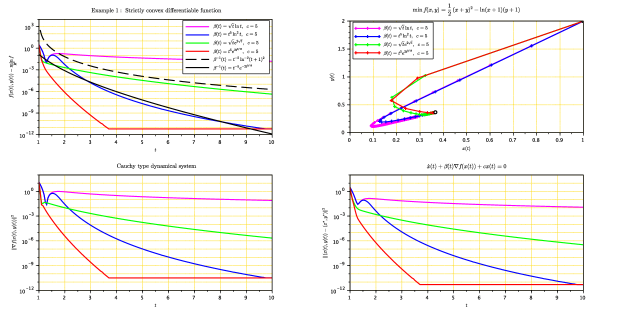
Figure 1: Evolution of convergence rates for values, trajectories and gradients when $c=5$ is fixed and $\beta(t)$ changes expressions from logarithm to exponential. Note, see the figure at the top left, that convergence rates respect our predictions in the results mentioned above.

4 Example for comparison of the convergence rate

Example 1.

Take $f:]-1,+\infty[^{2}\to{\mathbb{R}}$ which is defined for $x=(x_{1},x_{2})$ by

$$f(x)=\frac{1}{2}(x_{1}+x_{2})^{2}-\ln(x_{1}+1)(x_{2}+1).$$

The function $f_{1}$ is strictly convex with gradient $\nabla f(x)=\begin{bmatrix}x_{1}+x_{2}-\frac{1}{x_{1}+1}\\ x_{1}+x_{2}-\frac{1}{x_{2}+1}\end{bmatrix}$ and Hessian $\nabla^{2}f(x)=\begin{bmatrix}1+\frac{1}{(x_{1}+1)^{2}}&1\\ 1&1+\frac{1}{(x_{2}+1)^{2}}\end{bmatrix}$, so the unique minimizer of $f$ is $x^{*}=\left((\sqrt{3}-1)/2,(\sqrt{3}-1)/2\right)$.

The corresponding trajectories to the system (2) are depicted in Figure 1. We note that the convergence rates of the values and gradients in this numerical test are consistent with those predicted in Corollaries 3 and 4, while the convergence rates of the gradients are clearly stronger than those predicted theoretically. Let us consider the times-second-order systems, treated in the very recent papers:

$$\begin{array}[]{lll}\hbox{(TRAL)}&&\dot{x}(t)+2t^{2}\ln^{2}t\nabla f\left(x(t)\right)+5x(t)=0,\\ \hbox{(TRAE)}&&\dot{x}(t)+2t^{2}e^{2t^{9/10}}\nabla f\left(x(t)\right)+5x(t)=0,\\ \hbox{(TRISAL)}&&\ddot{x}(t)+5\dot{x}(t)+2t^{2}\ln^{2}t\nabla f\left(x(t)\right)+5x(t)=0,\hbox{ see \cite[cite]{[\@@bibref{Number}{BCR1}{}{}]}, }\\ \hbox{(TRISAE)}&&\ddot{x}(t)+5\dot{x}(t)+2t^{2}e^{2t^{4/5}}\nabla f\left(x(t)\right)+5x(t)=0,\hbox{ see \cite[cite]{[\@@bibref{Number}{BCR1}{}{}]}, }\\ \hbox{(TRISG)}&&\ddot{x}(t)+5t^{-4/5}\dot{x}(t)+\nabla f\left(x(t)\right)+t^{-8/5}x(t)=0,\hbox{ see \cite[cite]{[\@@bibref{Number}{ABCR-JDE}{}{}]}, }\\ \hbox{(TRISH)}&&\ddot{x}(t)+5t^{-4/5}\dot{x}(t)+\nabla f\left(x(t)\right)+2\nabla^{2}f\left(x(t)\right)\dot{x}(t)+t^{-8/5}x(t)=0,\hbox{ see \cite[cite]{[\@@bibref{Number}{ABCR-JDE}{}{}]}.}\end{array}$$

By comparing the two times-first-order systems, (2) where $\beta(t)$ is either equal to $2t^{2}\ln^{2}t$ or $2t^{2}e^{2t^{9/10}}$, with those of second order, we are surprised (see Figure 2) by the better rate of convergence brought by these two reduced and inexpensive systems.

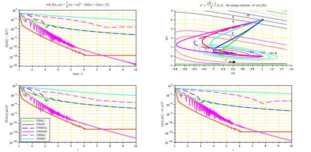
Figure 2: Here, we compare the convergence rates of values, trajectories and gradients for our first order system (LABEL:continuous_system) and those of the second order of recent references [3, 14].

5 Discussion and Conclusion

In this paper we first study a first order dynamical system

$$\dot{x}(t)+\beta(t)\nabla\left(f+\dfrac{c}{2\beta(t)}\lVert\cdot\rVert^{2}\right)(x(t))=0$$

which can be viewed as a Cauchy system with a time rescaling parameter on the gradient of the objective function and a Tikhonov regularization term. This dynamical system makes it possible to maintain the rate for convergence of values for generated trajectory for systems without Tikhonov regularization. We obtain moreover a similar rate for convergence of the norm-square of the associated gradients towards the origin. Another original new assertion of our system is the strong convergence of the generated trajectory towards the minimum norm solution of the objective function.

It would be a novelty in the literature to achieve a good speed of convergence for values and gradients with a time first order system, because recent papers [14, 15] have achieved the same speeds of convergence with the time second order differential systems:

$$\ddot{x}(t)+\alpha\,\dot{x}(t)+\beta(t)\nabla f(x(t))+cx(t)=0,$$

$$\ddot{x}(t)+\alpha\,\dot{x}(t)+\delta\nabla^{2}f(x(t))\dot{x}(t)+\beta(t)\nabla f(x(t))+cx(t)=0.$$

As desired, future theoretical and numerical study may be the subject of further work which focus on extending the study of the performance of systems associated with other penalization functions than $\frac{1}{2}\|\cdot\|^{2}$. More precisely, consider

$$\dot{x}(t)+\beta(t)\nabla\left(f+\dfrac{1}{\beta(t)}g\right)(x(t))=0$$

in order to solve with the same performance the two level hierarchical minimization problem: $\min g(x)$ under constraints the solution-set of the convex function $f$.

Appendix A

The following Lemma provides an extended version of the classical gradient lemma which is valid for differentiable convex functions. The following version has been obtained in [7, Lemma 1], [8]. We reproduce its proof for the convenience of the reader.

Lemma 5.

Let $f:\mathcal{H}\to{\mathbb{R}}$ be a convex function whose gradient is $L$-Lipschitz continuous. Let $s\in]0,1/L]$. Then for all $(x,y)\in\mathcal{H}^{2}$, we have

$$f(y-s\nabla f(y))\leq f(x)+\left\langle\nabla f(y),y-x\right\rangle-\frac{s}{2}\|\nabla f(y)\|^{2}-\frac{s}{2}\|\nabla f(x)-\nabla f(y)\|^{2}.$$ (32)

In particular, when ${\rm argmin}\kern 1.43994ptf\neq\emptyset$, we obtain that for any $x\in\mathcal{H}$

$$f(x)-\min_{\mathcal{H}}f\geq\frac{1}{2L}\|\nabla f(x)\|^{2}.$$ (33)

Proof.

Denote $y^{+}=y-s\nabla f(y)$. By the standard descent lemma applied to $y^{+}$ and $y$, and since $sL\leq 1$ we have

$$f(y^{+})\leq f(y)-\frac{s}{2}\left(2-Ls\right)\|\nabla f(y)\|^{2}\leq f(y)-\frac{s}{2}\|\nabla f(y)\|^{2}.$$ (34)

We now argue by duality between strong convexity and Lipschitz continuity of the gradient of a convex function. Indeed, using Fenchel identity, we have

$$f(y)=\langle\nabla f(y),\,y\rangle-f^{*}(\nabla f(y)).$$

$L$-Lipschitz continuity of the gradient of $f$ is equivalent to $1/L$-strong convexity of its conjugate $f^{*}$. This together with the fact that $(\nabla f)^{-1}=\partial f^{*}$ gives for all $(x,y)\in\mathcal{H}^{2}$,

$$f^{*}(\nabla f(y))\geq f^{*}(\nabla f(x))+\langle x,\,\nabla f(y)-\nabla f(x)\rangle+\frac{1}{2L}\lVert\nabla f(x)-\nabla f(y)\rVert^{2}.$$

Inserting this inequality into the Fenchel identity above yields

$$f(y) \leq-f^{*}(\nabla f(x))+\langle\nabla f(y),\,y\rangle-\langle x,\,\nabla f(y)-\nabla f(x)\rangle-\frac{1}{2L}\lVert\nabla f(x)-\nabla f(y)\rVert^{2}$$

$$=-f^{*}(\nabla f(x))+\langle x,\,\nabla f(x)\rangle+\langle\nabla f(y),\,y-x\rangle-\frac{1}{2L}\lVert\nabla f(x)-\nabla f(y)\rVert^{2}$$

$$=f(x)+\langle\nabla f(y),\,y-x\rangle-\frac{1}{2L}\lVert\nabla f(x)-\nabla f(y)\rVert^{2}$$

$$\leq f(x)+\langle\nabla f(y),\,y-x\rangle-\frac{s}{2}\lVert\nabla f(x)-\nabla f(y)\rVert^{2}.$$

Inserting the last bound into (34) completes the proof. ∎

References

• [1] Attouch, H.: Variational Convergence for Functions and Operators, Appl. Math. Ser., Pitman Advanced Publishing Program, Boston (1984) https://doi.org/10.1137/S1052623493259616
• [2] Attouch, H.: Viscosity solutions of minimization problems, SIAM J. Optim. 6 (3), 769–806 (1996) https://doi.org/10.1137/S1052623493259616
• [3] Attouch, H., Balhag, A., Chbani, Z., Riahi, H.: Damped inertial dynamics with vanishing Tikhonov regularization: Strong asymptotic convergence towards the minimum norm solution, J. Differential Equations 311, 29–58 (2022) https://doi.org/10.1016/j.jde.2021.12.005
• [4] Attouch, H., Balhag, A., Chbani, Z., Riahi, H.: Fast convex optimization via inertial dynamics combining viscous and Hessian-driven damping with time rescaling, Evol. Equ. Control Theory 11, 487–514 (2022) https://doi.org/10.3934/eect.2021010
• [5] Attouch, H., Balhag, A., Chbani, Z., Riahi, H.: Accelerated gradient methods combining Tikhonov regularization with geometric damping driven by the Hessian, Appl. Math. Optim. 88, 29 (2023). https://doi.org/10.1007/s00245-023-09997-x
• [6] Attouch, H., Boţ, R.I., Nguyen, D.-K.: Fast convex optimization via closed-loop time scaling of gradient dynamics, arXiv preprint https://doi.org/10.48550/arXiv.2301.00701 (2023)
• [7] Attouch, H., Chbani, Z., Fadili, J., Riahi, H.: First order optimization algorithms via inertial systems with Hessian driven damping, Math. Program. 193, 113–155 (2022) https://doi.org/10.1007/s10107-020-01591-1
• [8] Attouch, H., Chbani, Z., Fadili, J., Riahi, H.: Convergence of iterates for first-order optimization algorithms with inertia and Hessian driven damping, Optimization 72, 1199–1238 (2023) https://doi.org/10.1080/02331934.2021.2009828
• [9] Attouch, H., Chbani, Z., Riahi, H.: Fast proximal methods via time scaling of damped inertial dynamics, SIAM J.Optim. 29 (3), 2227–2256 (2019) https://doi.org/10.1137/18M1230207
• [10] Attouch, H., Chbani, Z., Riahi, H.: Fast convex optimization via time scaling of damped inertial gradient dynamics, Pure Appl. Funct. Anal. 6, 1081–1117 (2021)
• [11] Attouch, H., Cominetti, R.: A dynamical approach to convex minimization coupling approximation with the steepest descent method, J. Differential Equations 128 (2), 519–540 (1996) https://doi.org/10.1006/jdeq.1996.0104
• [12] Attouch, H., Czarnecki, M.O.: Asymptotic behavior of coupled dynamical systems with multiscale aspects, J. Differential Equations 248, 1315–1344 (2010) https://doi.org/10.1016/j.jde.2009.06.014
• [13] Attouch, H., Czarnecki, M.O.: Asymptotic behavior of gradient-like dynamical systems involving inertia and multiscale aspects, J. Differential Equations 262 (3), 2745–2770 (2017) https://doi.org/10.1016/j.jde.2016.11.009
• [14] Bagy, A.C., Chbani, Z., Riahi, H.: The heavy ball method regularized by Tikhonov term. Simultaneous convergence of values and trajectories, Evol. Equ. Control Theory 12 (2), 687–702 (2023) https://doi.org/10.3934/eect.2022046
• [15] Bagy, A.C., Chbani, Z., Riahi, H.: Strong convergence of trajectories via inertial dynamics combining Hessian-driven damping and Tikhonov regularization for general convex minimizations, Numer. Funct. Anal. Optim. 44, 1481–1509 (2023) https://doi.org/10.1080/01630563.2023.2262828
• [16] Boţ, R.I., Karapetyants, M.A.: A fast continuous time approach with time scaling for nonsmooth convex optimization, Adv. Cont. Discr. Mod. 73 (2022) https://doi.org/10.1186/s13662-022-03744-2
• [17] Brézis, H.: Analyse Fonctionnelle, Masson (1983)
• [18] Cabot A.: Proximal point algorithm controlled by a slowly vanishing term: Applications to hierarchical minimization, SIAM J. Optim. 15, 555–572 (2005) https://doi.org/10.1137/S105262340343467X
• [19] Chadli O, Chbani Z, Riahi H.: Equilibrium problems with generalized monotone bifunctions and applications to variational inequalities. J. Optim. Theory Appl. 105 , 299–323 (2000) https://doi.org/10.1023/A:1004657817758
• [20] Morozov, V.A.: Methods of solving incorrectly posed problems, Springer Verlag, New York (1984) https://doi.org/10.1007/978-1-4612-5280-1
• [21] Tikhonov, A.N.: On the solution of ill-posed problems and the method of regularization, Soviet Math. Dokl. 4, 1035–1038 (1963)
• [22] Tikhonov, A.N.: On the regularization of ill-posed problems, Soviet Math. Dokl. 4 , 1624–1627 (1963)
• [23] Tikhonov, A.N., Leonov, A., Yagola, A. : Nonlinear ill-posed problems, Chapman and Hall, London (1998)