A Fast Convergence Algorithm for Iterative Adaptation
of Feedforward Controller Parameters*

Abstract

Feedforward control is a viable option for enhancing the response time and control accuracy of a wide variety of systems. Nevertheless, it is not able to compensate for the effects produced by modeling errors or disturbances. A solution to improve the feedforward performance is the use of an adaptation law that modifies the parameters of the feedforward control. In the case where real-time feedback is not possible, a solution is a run-to-run numerical optimization method that is fed with a cost based on a measured signal. Although the effectiveness of this approach has been demonstrated, its performance is hindered by slow convergence. In this paper, we present an algorithm based on Pattern Search and Adaptive Coordinate Descent methods that makes use of the sensitivity of the feedforward controller to its parameters so that the convergence speed improves significantly. Like many algorithms, this is a local strategy so the algorithm might converge to a local minimum. Therefore, we present two versions, one without a learning rate and one with it. To compare them and to demonstrate the effectiveness of the algorithm, simulated results are shown on a well-known control problem in electromechanics: the soft-landing control of electromechanical switching devices.

I Introduction

Feedforward control is an important element in control systems, offering immediate responses to reference changes or known disturbances. Despite their advantages, feedforward controllers alone are not robust to design errors, modeling errors, or system changes. To address these limitations, various complementary strategies exist, including conventional feedback controllers with observers [1], learning algorithms [2], and parameter adjustments based on measured variables [3].

As can be seen, there are many solutions when the state variables can be measured. However, in some situations these measurements are not feasible, either because the sensor is more expensive than the device to be controlled, or because such measurements are not accessible. In our previous work [4] we proposed a solution to this situation in impact reduction control of electromechanical switching devices. Using an alternative measurement, such as impact velocity in simulation or a measure of impact sound in real-world experiments, a cost is calculated. Then, using a black box approach, the parameters of the feedforward controller are iteratively modified. The initial results demonstrate the efficacy of the control structure, but we believe that the convergence of the black box proposal in [4] can be improved. The black box algorithm is a Pattern Search [5] algorithm. It is one of the derivative-free optimizations and, as this type of methods, it has the advantages of not using derivatives or finite differences, only having to compare function values. It is very useful for the problem treated, since the relationship between the input and output of the black box is unknown. As an improvement, in [6], a dimensionality reduction and a change of coordinate system for the optimization algorithm are proposed. The results confirm the effectiveness and highlight the potential for improvement.

In this line, [7] presents an Adaptive Coordinate Descent algorithm. The strategy involves periodically updating the coordinate system by a Covariance Matrix Adaptation Evolution Strategy (CMA-ES) and Adaptive Encoding to decompose the problem into as many one-dimensional problems as there are dimensions in the general problem. While the general concept can be useful in some applications, the use of a CMA-ES can be counterproductive in control field. As concluded by the authors in [8], there are fundamental limitations to the possibilities of self-adaptation in evolutionary strategies. The number of function evaluations required to reliably achieve a significant change is high. The function evaluations they consider are 10$q$ (where $q$ is the problem dimension), 30$q$ for a real-world search problem, and 100$q^{2}$ for complete adaptation.

In terms of one-dimensional search, the authors of [7] suggest free-derivative methods (such as Pattern Search methods) or the use of gradients. Gradient methods are a strong powerful tool, but in our problem, the objective function equation is unknown and cannot be evaluated directly. However the use of subgradients may be an option. In this line, a solution could be sign gradient descent methods, first introduced in the RProp algorithm [9]. The RProp (Resilient Propagation) algorithm is a gradient descent algorithm that uses only the signs of the gradients to compute updates. Although it is a gradient method, the computational load is low because it is not necessary to compute the gradient, only its sign. Also, they may allow to reach minima other than the closest minimum of the initial condition, which makes these algorithms usable for global optimization. Nevertheless, adjusting their initial parameters and hyperparameters can be a challenging task. In contrast, gradient descent methods set an adaptive step size without the need for hyperparameters. A popular and effective method is the Polyak step size. This method is coupled with others [10] based on momentum acceleration, moving averaged gradient or stochastic methods [11], among others. Furthermore, its use in the subgradient method is common.

To address the problems highlighted above, in this paper we present a new algorithm that performs the functions of the black box. The proposed new algorithm is composed to a technique based on the sensitivity of the feedforward law that decomposes the initial $q$-dimensional problem into $q$ one-dimensional problems, a method that selects the descent coordinate and makes movements in this direction, and a learning rate that enhances the algorithm performance. The main contribution is the transfer of optimization techniques more commonly used in other fields to the field of control, in particular the combination of free derivative algorithms and gradient descent methods.

The paper is structured as follows. Section II presents the work control structure and the first step to improve the convergence of the feedback loop. Section III develops the proposed algorithm in three parts: the basis change, the search method, and the subgradient learning rate. Section IV summarizes everything related to the simulation experiments: the dynamic system and feedforward control used, the simulation conditions, and the results that show the improvements. Finally, the conclusions are discussed in Section V.

II Background of the control system

Figure 1: General control diagram. The subscript $k$ denotes the variables of the $n$-th evaluation of the run-to-run adaptation law. The feedforward block computes $u_{f{\!}f}$ from the parameter vector $p$ and the desired reference signal $ref$. The adaptation law updates $p$ using the cost $f$, which is derived from the measurable output $y$.

The first proposal [4] focuses on the control of systems with differentially flat dynamical models. An $n$-th order system is differentially flat if the $n$-th derivative of the output is the first where the input appears explicitly [12]. This property allows the design of a feedforward controller by model inversion. However, despite its simplicity, errors in the model or parameter identification can significantly affect the accuracy of the controller. Therefore, the inclusion of a feedback loop is essential. The interest of this proposal lies in addressing scenarios when the measurement of the signal to be controlled is not available. To address this challenge, a system measurement that can be processed and converted into a performance indicator is selected as the feedback measurement. Closing the feedback loop requires a block that relates the performance indicator to the primary control loop. The proposed control structure is schematized in Fig. 1. However, it can often be difficult to find a function that effectively links these two aspects and can be implemented online. As a solution, [4] proposes a pattern search algorithm uses the performance indicator as a cost function to optimize the feedforward parameters.

After the initial proposal, future work has focused on improving the convergence speed of the method. [6] addresses this by applying dimensionality reduction techniques to the parameter set. This method proposes two techniques based on the sensitivity of the controller to the parameters. The first one involves optimizing only $r<q$ most sensitive parameters of $p\in\mathbb{R}^{q}$. The second technique aims to reduce an alternative orthogonal $q$ coordinate system. Using the sensitivity of the feedforward controller, the Fisher matrix information is computed to construct a basis change matrix composed of Fisher matrix information eigenvectors. The main idea is to concentrate all the information into a smaller number of parameters to increase the controller accuracy when the dimensionality of the problem is reduced. Both proposals in that work use a fixed basis change matrix based on the nominal value of the feedforward controller parameters. However, we suggest the possibility of periodically updating the reduced parametric basis.

III New algorithm

The proposed algorithm tries to solve two different issues. The first one is to answer the questions of [6], i.e., how often the reduced parametric basis should be updated and what is the appropriate size of the search dimension at each update. The second is to be able to adapt when the error between actual and optimal parameters is significantly large.

For the first issue, following the idea presented in [7], the algorithm combines a simple optimization method, e.g., some successive line searches by coordinates, with a method that periodically adapts a coordinate system. This method aims to decompose the problem into separable functions that set the control output $u_{f{\!}f}(t,\theta)$, where $\theta$ is a set of auxiliary parameters. This set can be the parameter vector $p$, a subset of this vector or a function of them, e.g. the normalized parameters by their nominal parameters $p^{nom}$, $\theta=p\oslash p^{nom}$, where $\oslash$ denotes element-wise division. For the second issue, the idea is to add to the equation that calculates the next point with a learning rate parameter based on subgradient methods.

III-A An alternative orthogonal coordinate system

In our proposal, we use the second method proposed in [6] as the technique that adapts the coordinate system. In short, this technique is based on calculating the new coordinate system which keeps constant the integral-square deviation of $u_{f{\!}f}$ with respect to the nominal input $\theta^{nom}$, $D(\theta)$,

$$D(\theta)=\frac{1}{2}\int_{t_{0}}^{t_{\mathrm{f}}}\big{(}u_{f{\!}f}(\tau,\theta)-u_{f{\!}f}(\tau,\theta^{nom})\big{)}^{2}\,\mathrm{d}\tau,$$ (1)

By a simplification of the Taylor expansion around the nominal parameter vector, the integral-square deviation of $u_{f{\!}f}$ with respect to the nominal input is approximately given by the quadratic form

$$D(\theta)\approx\frac{1}{2}\,\delta\theta^{\intercal}\,\mathcal{F}({\theta^{nom}})\,\delta\theta,$$ (2)

where $\delta\theta=\theta-\theta^{nom}$, and $\mathcal{F}({\theta^{nom}})\in\mathbb{R}^{q\times q}$ is the Fisher matrix, which can be calculated from the sensitivity of the feedforward law to the vector $\theta$ of the control parameters, $S(t,\theta)\in\mathbb{R}^{1\times q}$, as follows:

$$S(t,\theta)=\dfrac{\partial u_{f{\!}f}(t,\theta)}{\partial\theta},$$ (3)

$$\mathcal{F}({\theta})=\int_{t_{0}}^{t_{\mathrm{f}}}\mathopen{}\mathclose{{}\left[S(t,\theta)^{\intercal}\,S(t,\theta)}\right]\,\mathrm{d}\tau.$$ (4)

On the other hand, the Fisher matrix could be decomposed into the matrix of its eigenvalues, $\Lambda$, and its eigenvectors, $V$.

$$D(\theta)\approx\frac{1}{2}\,\delta\theta^{\intercal}\,{\mathcal{F}}({\theta^{nom}})\,\delta\theta=\frac{1}{2}\,\delta\theta^{\intercal}\,V\,\Lambda\,V^{\intercal}\,\delta\theta.$$ (5)

Through a variable change, the transformation between the old coordinate system, $\theta$, and the new coordinate system, $X$, can be performed using a matrix whose columns are the eigenvectors of the Fisher matrix.

$$X=V^{\intercal}\,\theta\ \Longleftrightarrow\ \theta=V\,X.$$ (6)

This transformation not only allows the problem to be decomposed into separable functions, but also provides an orthogonal coordinate system sorted by the average sensitivity over time of the feedforward law to the new parameters $\bar{S}(X)$.

$$\bar{S}(X_{(1)})>\bar{S}(X_{(2)})>\dotsc>\bar{S}(X_{(q)}),$$ (7)

where $X_{(i)}$ denotes the $i$-th element of $X$.

III-B Search of the descending coordinate and line search

Figure 2: General rule for the movements of the new algorithm.. The “min” condition indicates whether a local minimum has been found at the current coordinate. “d” represents the evaluated coordinate. “Ev. coordinate” encompasses the evaluation of the central point (currently the best) and the two side points of the corresponding coordinate. “d+1” involves cyclically succeeding to the next coordinate. “Prop.” refers to propagation in the downward direction of the current coordinate. “Init. pattern” entails recalculating the basis change matrix (if necessary) and restarting the pattern. Note that if we look only at the left arrows, the movements of the Pattern Search are represented.

Once we have a coordinate system that we assume has a low correlation between its coordinates, we can apply a successive linear coordinate search. To do this, first, the coordinate with further decrease in cost has been found, and then a method that search the minimum at the coordinate should be selected. The proposal for selecting the coordinate of greatest descent is based on Pattern Search. A pattern of $(2q+1)$ points is created with the center point being the lowest cost evaluated point, and two side points at each coordinate. Due to the coordinate are sorted by the sensitivity of the feedforward law, we assume the first evaluations can generate the greatest improvements. Once a cost-improving coordinate has been found, the algorithm continues to look for lower cost points in that direction by a method that embraces the philosophy of sign gradient descent algorithms. Thus, it is not necessary to complete the pattern to update the best point. When the next point does not improve the cost, assume a minimum is found and evaluate a new pattern.

To obtain the new pattern, a new orthogonal coordinate system is calculated and the search starts again at the most sensitive coordinate, i.e., the first new coordinate. The only exception is when the algorithm has been moved to the first coordinate. In this case a new pattern is not calculated and the algorithm continues the pattern at the second coordinate. The main reason is not to convert the algorithm into a single gradient search method in which the descendent coordinate is calculated though the coordinate that most modified $u_{f{\!}f}$, because the speed of convergence could be reduced to the lack of opportunity to directly find a new best point. In Fig. 2 outlines the movement rules. As can be inferred, if the initialization pattern block (“Init. pattern”) is reached with the left arrows, it is not necessary to recalculate the basis change matrix. This is because, after evaluating the entire pattern, the best point remains the initial one, and consequently, the basis change matrix remains unchanged.

As for the step size, $s\in\mathbb{R}$, with the same philosophy as Pattern Search and RProp, when we seem to be moving in a good direction, the step size should be increased to get to the optimal point faster, and when we have just fallen over a minimum, the step size should be decreased to allow us to get closer to the minimum cost. In short, the next point to evaluate can be calculated as

$$X_{k+1}=X_{\mathrm{best}}+s_{k}\vec{u_{k}};$$ (8)

$$s_{k}=\Biggl{\{}\begin{array}[]{cc}\max(\alpha_{\mathrm{con}}\,s_{k-1},\,s_{\mathrm{min}})&\mathrm{if}\,f(X_{k})>f(X_{\mathrm{best}})\\ \min(\alpha_{\mathrm{exp}}\,s_{k-1},\,s_{\mathrm{max}})&\mathrm{if}\,f(X_{k})\leq f(X_{\mathrm{best}})\end{array}$$ (11)

where $\vec{u_{k}}$ is the unitary vector with angle equal a system coordinate and desired direction. The values $\alpha$ are constants such that $0\,<\,\alpha_{\mathrm{con}}\,<\,1\,<\,\alpha_{\mathrm{exp}}$. The values $s_{\mathrm{min}}$ and $s_{\mathrm{max}}$ are the minimum and maximum allowed step sizes, respectively.

III-C Subgradient learning rate

Although with this new heuristic we have addressed the questions regarding updating the reduced parametric basis, like the predecessor algorithms, it is useful only if the target point is near the initial estimation or the objective function is globally convex. If this is not true, it may converge to a local minimum and not reach the global minimum. In order to try to solve this problem, we propose to modify (11) as a modified gradient method

$$X_{k+1}=X_{\mathrm{best}}+(\vec{u_{k}}-\eta_{k}\,g_{k})\,s_{k},$$ (12)

where $g_{k}\in\mathbb{R}^{q}$ is the gradient, and $\eta_{k}\in\mathbb{R},\,\eta_{k}>0$, is another step size in iteration $k$. However, given that the objective function is unknown (only its evaluated values are available), and we cannot assume the objective function is a continuous differentiable equation, the algorithm is treated as a subgradient method. As described in [10], a technique to calculate $\eta_{k}$ is to minimize the squared distance between $X_{k+1}$ and the optimal point $X^{*}$.

$$\eta_{k}=\arg\min_{\eta}\|X_{k+1}-X^{*}\|^{2}$$ (13)

$$\eta_{k}=\arg\min_{\eta}\|X_{k}+(\vec{u_{k}}-\eta_{k}\,g_{k})\,s_{k}-X^{*}\|^{2}.$$ (14)

Expanding the squared norm, the equation to be minimized is

$$\|X_{k}-X^{*}\|^{2}+\|s_{k}\vec{u_{k}}\|^{2}-2\,\|s_{k}\vec{u_{k}}\|\,\|\eta_{k}g_{k}s_{k}\|\cos{\alpha}+\\ \|\eta_{k}g_{k}s_{k}\|^{2}+2\,\|X_{k}-X^{*}\|\|s_{k}\vec{u_{k}}-\eta_{k}s_{k}g_{k}\|\cos{\gamma},$$ (15)

where $\alpha$ and $\gamma$ are the angle between $\vec{u_{k}}$ and $g$, i.e., between the coordinate of movement and the gradient, and the angle between $X_{k}-X^{*}$ and $s_{k}\vec{u_{k}}-\eta_{k}s_{k}g_{k}$, i.e, the descent direction and the theoretical next step, respectively. By the relationship

$$\cos{\gamma}=\frac{\|s_{k}\vec{u_{k}}\|\cos{\alpha}-\|\eta_{k}g_{k}s_{k}\|}{\|s_{k}\vec{u_{k}}-\eta_{k}s_{k}g_{k}\|},$$ (16)

and considering we only want this extra term to acts when the algorithm falls into a local minimum or the convergence is too slow, i.e., assuming $\|X_{k}-X^{*}\|\gg s_{k}$, (15) is reduced to

$$\|X_{k}-X^{*}\|^{2}-2\,\|s_{k}\vec{u_{k}}\|\,\|\eta_{k}g_{k}s_{k}\|\cos{\alpha}+\\ \|\eta_{k}g_{k}s_{k}\|^{2}-2\,\|X_{k}-X^{*}\|\,\|\eta_{k}s_{k}g_{k}\|.$$ (17)

With the previous assumption, knowing that $s_{k}$ is an scalar and $\|\vec{u_{k}}\|=1$, the solution of the minimization is

$$\eta_{k}=\frac{2\mathopen{}\mathclose{{}\left(s_{k}\|g_{k}\|\|X_{k}-X^{*}\|+s_{k}^{2}\|g_{k}\|\cos{\alpha}}\right)}{2s_{k}^{2}\|g_{k}\|^{2}}\,\pm\\ \frac{\sqrt{4\mathopen{}\mathclose{{}\left(s_{k}^{4}\|g_{k}\|\cos{\alpha})^{2}+2s_{k}^{3}\|g_{k}\|^{2}\|X_{k}-X^{*}\|}\right)}}{2s_{k}^{2}\|g_{k}\|^{2}}.$$ (18)

Although the point $X^{*}$ is unknown, if we consider an objective function with a general convex behavior we can suppose $\|g\|\,\|X_{k}-X^{*}\|>f(X_{k})-f^{*}$, where $f^{*}$ is the minimum cost. If we substitute $\|g\|\,\|X_{k}-X^{*}\|=f(X_{k})-f^{*}$, we obtain an upper bound of the minimization, and $\eta_{k}$ is calculated as

$$\eta_{k}=\frac{f(X_{k})-f^{*}}{s_{k}\|g_{k}\|^{2}}+\frac{\cos{\alpha}}{\|g_{k}\|}\\ \pm\frac{1}{\|g_{k}\|}\sqrt{\cos{\alpha}^{2}+2\frac{(f(X_{k})-f^{*})\cos{\alpha}}{s_{k}\|g_{k}\|}}.$$ (19)

Since we are moving in only one coordinate, we consider $\alpha=0$, i.e., we assume that the coordinate is the descent direction. This assumption introduces an error, but, of the two solutions obtained for $\eta_{k}$ choosing the subtraction operation in the $\pm$ operation provides a conservative solution and smaller error.

Due to the low information of the gradient at each coordinate and the possible unsmoothed result, $f(X_{k})$ and $g$ are replaced by average values.

$$\tilde{f}_{k}=\beta\tilde{f}_{k-1}+(1-\beta)f(X_{k}),$$ (20)

$$\tilde{g}_{k}=\sqrt{\beta\tilde{g}_{k-1}^{2}+(1-\beta)\mathopen{}\mathclose{{}\left(\frac{f(X_{k})-f(X_{k-1})}{||X_{k})-X_{k-1}||}}\right)^{2}},$$ (21)

where $\beta<1$ is a positive constant that acts as a decay factor.

Working with an average value of the cost, $\tilde{f}_{k}$, local minima, in which the objective function is not globally convex, gives higher values, causing the algorithm to avoid these points. The interest of $\tilde{g}$ is to mitigate excessively oscillating learning rates. This technique is already used in other algorithms, such as Root Mean Square Propagation (RMSProp) and other stochastic gradient descent algorithms.

The only term that remains to be defined is $f^{*}$. This value can be considered a constant and if the real value in not know, $f^{*}=0$ is adequate on many situations, but it is usually a strong assumption. Alternatively, it can be considered as an iteration-dependent target value. This idea is more interesting in our case, because we want the additional terms to help (11) when the convergence is slower due to the evaluated point being far from the solution point. For this reason the different between $\tilde{f}(X_{k})$ and $f^{*}$ is saturated. We define the next function

$$\delta f=\max(\tilde{f}_{k}-f_{k}^{*},0).$$ (22)

Finally, taking into account that $g_{k}=-\|g_{k}\|$ in the descent direction, the next point to evaluate can be calculate as

$$X_{k+1}=X_{\mathrm{best}}+\\ \Bigg{(}1+\Big{(}\frac{\delta f}{s_{k}\tilde{g}_{k}}+1-\sqrt{1+2\frac{\delta f}{s_{k}\tilde{g}_{k}}}\Big{)}\Bigg{)}\,s_{k}*\vec{u_{k}};$$ (23)

Note, if $\tilde{f}_{k}\leq f_{k}^{*}$, i.e., $ff=0$, both (11) and (23) are the same equation, and, if $s_{k}\thickapprox 0$, (23) is very similar to applying Polyak step size.

IV Simulated results

In this section we present through simulation an example of operation in a non-linear system based on the dynamics of electromechanical switching devices. These devices experience significant collisions at the end of switching operations, posing a continuous control challenge that has previously been addressed by soft landing controls. To illustrate the benefits of the new feedback algorithm, we discuss the improvements achieved over our previous work [6].

IV-A System dynamics

The dynamical model used for the simulated experiments is based on a single-coil reluctance actuator. This actuator is affected by two types of forces: passive elastic forces, which can generally be modeled as ideal springs, and magnetic force. The magnetic force is generated when current flows through the coil, causing an inner fixed core to become magnetized and attract the movable core. The typical method of supplying the actuator with power is by providing a voltage. We describe the dynamics of the system using a state-space model, where the voltage $u$, is the input to our system, the position $z$ is the output, and velocity $v$ and magnetic flux linkage $\lambda$ are auxiliary state variables. The state equations are defined as

$$\dot{z} =v,$$ (24)

$$\dot{v} =\frac{1}{m}\,\mathopen{}\mathclose{{}\left(-k_{\mathrm{s}}\,\mathopen{}\mathclose{{}\left(z-z_{\mathrm{s}}}\right)-\frac{1}{2}\,\lambda^{2}\,\frac{\partial\mathcal{R}}{\partial z}}\right),$$ (25)

$$\dot{\lambda} =-R\,\lambda\,\mathcal{R}(z,\lambda)+u,$$ (26)

where $m$, $k_{\mathrm{s}}$, $z_{s}$, $R$, and $\mathcal{R}$ are the moving mass, the spring stiffness, the spring resting position, the coil resistance, and an auxiliary function based on the magnetic reluctance concept, respectively. This magnetic reluctance considers the phenomena of magnetic saturation and flux fringing in the model

$$\mathcal{R}(z,\lambda)=\frac{\kappa_{1}}{1-|\lambda|/\kappa_{2}}+\kappa_{3}+\frac{\kappa_{4}\,z}{1+\kappa_{5}\,z\,\log(\kappa_{6}/z)},$$ (27)

where $\kappa_{1}$, $\kappa_{2}$, $\kappa_{3}$, $\kappa_{4}$, $\kappa_{5}$, and $\kappa_{6}$ are positive constants. Overall, the system dynamics depends on $q=9$ uncertain parameters, which can be grouped in the parameter vector $p$.

$$p=\\ \mathopen{}\mathclose{{}\left[\,\,k_{\mathrm{s}}\,\,\,\,z_{\mathrm{s}}\,\,\,\,m\,\,\,\,\kappa_{1}\,\,\,\,\kappa_{2}\,\,\,\,\kappa_{3}\,\,\,\,\kappa_{4}\,\,\,\,\kappa_{5}\,\,\,\,\kappa_{6}\,\,}\right]^{\intercal}.$$ (28)

Note that the resistance $R$ is treated independently as a parameter without uncertainty, as it can be precisely measured. As explained in [4], the model (24)–(26) exhibits differential flatness and we can calculate the feedforward controller by inversion of the model

$$u\mathopen{}\mathclose{{}\left(z,\dot{z},\ddot{z},\dddot{z},p}\right)=R\,\mathcal{R}(z,\lambda,p)\,\lambda+\dot{\lambda},$$ (29)

where $\lambda=f_{\lambda}\mathopen{}\mathclose{{}\left(z,\dot{z},\ddot{z},p}\right)$, and $\dot{\lambda}=f^{\prime}_{\lambda}\mathopen{}\mathclose{{}\left(z,\dot{z},\ddot{z},\dddot{z},p}\right)$ are derived from (25).

IV-B Description of the simulated experiments

In a real world scenario, we determine the parameters of an electromechanical switching device through a cumbersome estimation process. However, due to manufacturing or other tolerances, we assume that not all devices are identical and that the parameters vary from device to device. The values of the estimated parameters, which may be representative of a typical solenoid actuator or electromagnetic relay, are shown in Table I.

TABLE I: Nominal parameter values

$k_{\mathrm{s}}$	$55\,\mathrm{N/m}$		$\kappa_{5}$	$1320\,\mathrm{m^{-1}}$
$z_{\mathrm{s}}$	$0.015\,\mathrm{m}$		$\kappa_{6}$	$9.73\cdot 10^{-3}\,\mathrm{m}$
$m$	$1.6\cdot 10^{-3}\,\mathrm{kg}$		$R$	$50\,\mathrm{\Omega}$
$\kappa_{1}$	$1.35\,\mathrm{H^{-1}}$		$z_{0}$	$10^{-3}\,\mathrm{m}$
$\kappa_{2}$	$0.0229\,\mathrm{Wb}$		$z_{\mathrm{f}}$	$0$
$\kappa_{3}$	$3.88\,\mathrm{H^{-1}}$		$t_{0}$	$0$
$\kappa_{4}$	$7.67\cdot 10^{4}\,\mathrm{H^{-1}/m}$		$t_{\mathrm{f}}$	$3.5\cdot 10^{-3}\,\mathrm{s}$

In order to be able to compare the results, the desired position trajectory ($ref(t)$ in Fig. 1), necessary for the feedforward control and for the calculation of the base change matrix, is designed, as in [6]. This trajectory is formulated as a $5$th-degree polynomial with the following boundary conditions:

$$z_{\mathrm{d}}(t_{0}) =z_{0}, \dot{z}_{\mathrm{d}}(t_{0}) =0, \ddot{z}_{\mathrm{d}}(t_{0}) =0,$$ (30)

$$z_{\mathrm{d}}(t_{\mathrm{f}}) =z_{\mathrm{f}}, \dot{z}_{\mathrm{d}}(t_{\mathrm{f}}) =0, \ddot{z}_{\mathrm{d}}(t_{\mathrm{f}}) =0,$$

where $t_{0}$ and $t_{\mathrm{f}}$ are the desired initial and final times of the switching operation, and $z_{0}$ and $z_{\mathrm{f}}$ are the desired initial and final positions, which correspond to the mechanical limits of the motion of the movable core.

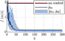
(a) ACD without learning rate.

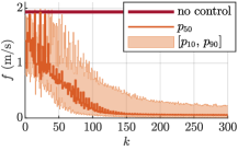
(b) Pattern Search with basis change ($r=4$).

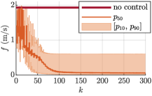
(c) Pattern Search with basis change ($r=2$).

Figure 3: Cost values with respect to the number of switching operations. Comparison between (a) the ACD algorithm without learning rate and the best results concerning (b) variability and (c) convergence speed of [6]. The cost without control is also represented.

In terms of variable measurements, the position of the movable core is not available. The electromechanical switching devices that we are considering are small in size and cheap, so using an expensive laser sensor for measurement would be impractical. Additionally, most of them are encapsulated within a protective housing, which impedes access to the component whose position needs to be known. In other works, during real world experimentation, the impact sound or the bounces are selected as indicators of control performance. In this simulations, as in [6], we consider the impact velocity such indicator

$$f=\mathopen{}\mathclose{{}\left\lvert{v_{\mathrm{c}}}}\right\rvert.$$ (31)

To emulate the real situation where the actual value of the parameters does not match the nominal values, 10 000 different trials have been conducted. In each trial, we initialize the feedforward law with the estimated parameters of a devices (see Table I). Due to the way the algorithm is set up as,

$$\theta={p}\oslash{p^{nom}},$$ (32)

the initial parameters take the value 1, i.e., $\theta_{1\,(i)}=\theta^{nom}_{(i)}=1\,\forall\,i$. To account for parameter variation, each component of the model parameter vector $p$ is randomly and independently perturbed by a certain percentage.

The results presented in this paper can be divided into three parts. First, to demonstrate the functionality of the ACD algorithm (without applying the learning rate) and to observe the improvement, we replicate the simulation conditions described in [6]. In this simulation, the control algorithm is executed for 300 switching operations in each trial, with parameter perturbations set to $5\,\%$. In other words, the parameters of the real device under consideration vary between $95\,\%$ and $105\,\%$ with a uniform probability distribution of the values in Table I. The second result is shown to test the influence of the learning coefficient. Finally, the third and last set of results addresses the impact of greater errors in the initial parameters. In this case, parameter perturbations are set at $25\,\%$. In this part, we compare the three algorithms again: the Pattern Search algorithm, the ACD algorithm without a learning rate, and the ACD algorithm with a learning rate.

IV-C Results

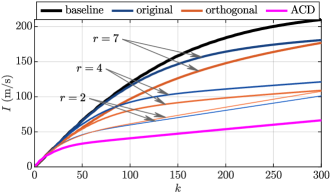
Figure 4: Integrated average cost with respect to the number of iterations. Comparison between the reduction methods of the previous paper and the new algorithm. Except ACD, all apply Pattern Search algorithm, original with the coordinate system without basis change, orthogonal with basis change, and baseline without basis change and without dimension reduction.

Fig. 3 shows the results for the first analysis. The graphs represent the evolution of the cost, $f$, with respect to each evaluation or switching operation, $k$. Due to the large number of simulations needed to reproduce the variability of the parameters between devices, the results are presented by the median ($p_{50}$) and the 10th and 90th percentiles ($p_{10}$ and $p_{90}$, respectively) of the distribution of values obtained for the 10 000 simulated experiments. For reference, the cost without control is also plotted. Fig. 3a shows the results when using the ACD algorithm, without applying the learning rate, to check its effectiveness and compare it with the previous results of [6] using the Pattern Search algorithm with an initial fixed change of the basis and a reduced dimensional coordinate system. Fig. 3b shows the results when only four dimensions are optimized, the situation with the least variability of results after 300 function evaluations. Fig. 3c shows the results when only two dimensions are optimized, the situation with the fastest convergence. From these results, we can conclude that the convergence is faster and the $p_{90}$ after 300 evaluations of the new algorithm is smaller. To facilitate comparisons between all the studied cases of the previous paper and the results obtained with the ACD algorithm, Fig. 4 shows the integrated (i.e., cumulative) average cost of each trial, denoted as $I$,

$$I_{k}=\sum_{i=1}^{k}\bar{f}_{k},$$ (33)

where $\bar{f}_{k}$ is the mean cost in the evaluation $k$ for the 10 000 simulated trials. The improvement is remarkable and, if we look at the trend, the intersection of the ACD curves with each other would be at infinity, i.e., the improvement is continuous over time.

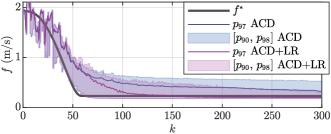
Figure 5: Cost values with respect to the number of switching operations. Comparison between the ACD algorithm without subgradient learning rate and ACD with learning algorithm.

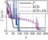
(a)

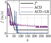
(b)

Figure 6: Effect of the learning rate. Evolution of $f$ in single processes. (a) Process with slow convergence. (b) Process with convergence to an unacceptable cost

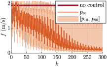
(a) Pattern Search with basis change ($r=4$).

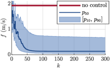
(b) ACD without learning rate.

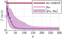
(c) ACD with learning rate.

Figure 7: Cost values with respect to the number of switching operations. The perturbation of the parameters is $25\,\%$.

To demonstrate the effect of the learning rate, the simulation is repeated with the same parameters for each trial. The function $f^{*}$ is calculated using the $p_{90}$ of the results ($p_{90}$ of Fig. 3a). Thus, the processes that do not require the learning rate, i.e., those at or below the 90th percentile, will remain unaffected. Fig. 5 shows the 90th, 97th and 98th percentiles ($p_{90}$, $p_{97}$ and $p_{98}$) for both processes, without (ACD) and with learning rate (ACD+LR). As expected, the evolution of $p_{90}$ is identical in both cases, and as the percentile gets higher, the algorithm with learning rate achieves better results with fewer evaluations. If we look at $p_{97}$, the ACD with learning rate reaches the target in less than 150 evaluations, while the version without learning rate does not reach it even after 300 evaluations. Additionally, Fig. 6 shows the $f$ evolution of two individual processes. These plots show the effect of the learning rate in a process with slow convergence (Fig. 6a) and convergence to an unacceptable cost (Fig. 6b).

Finally, Fig. 7 shows the behavior of the three algorithms when the parameters are not so close to the right ones. Fig. 7a shows the results of the Pattern Search algorithm with basis change and optimizing only four dimensions. However, the $p_{10}$ and $p_{50}$ have similar values to the processes when the estimation of the initial parameters are between $5\%$, the $p_{90}$ offers much higher values. Fig. 7b shows the results of the ACD without learning rate. The conclusions are similar to the previous ones, but, in this case the $p_{90}$, although elevated, is better than with the Pattern Search, and even seems not to have converged yet. Fig. 7c shows the results of the complete new algorithm, ACD with learning rate. In this case $p_{90}$, after 150 evaluations, converges to comparable values to when the initial error in the parameters was within 5$\%$, instead of 25$\%$.

V Conclusions

In this work we have presented a new algorithm to adapt the parameters of a feedforward controller from an alternative measurement of the state variables of the system. The improvement with respect to our previous has been achieved both for small initial parameter errors and for larger errors, where the previous technique is not useful.The improvements have been obtained by integrating three concepts into the algorithm: a periodic basis change based on the sensitivity of the feedforward law, the search for an optimal point in one dimension using the philosophy of the Pattern Search algorithms and sign gradient methods, and the inclusion of a learning rate calculated using the concepts used in the subgradient methods. Additionally, with this new algorithm we answer the questions of our previous work, the periodicity of updating the basis and the number of dimensions to reduce, due to the fact that the ACD selects the minimum number of dimensions to improve the feedforward controller behavior.

As future work, we would like to perform a deep theoretical analysis, and address some questions, such as the possibility of a technique to estimate the target function $f^{*}$ or to solve certain assumptions. In addition, we also intend to perform real laboratory tests on different systems to verify that the experimental results agree with those observed in simulation and the generality of the method.

References

- [1] R. Schroedter, M. Roth, K. Janschek, and T. Sandner, “Flatness-based open-loop and closed-loop control for electrostatic quasi-static microscanners using jerk-limited trajectory design,” Mechatronics, vol. 56, pp. 318–331, 2018.
- [2] M. Grotjahn and B. Heimann, “Model-based feedforward control in industrial robotics,” The International Journal of Robotics Research, vol. 21, no. 1, pp. 45–60, 2002.
- [3] S.-S. Yeh and P.-L. Hsu, “An optimal and adaptive design of the feedforward motion controller,” IEEE/ASME transactions on mechatronics, vol. 4, no. 4, pp. 428–439, 1999.
- [4] E. Moya-Lasheras, E. Ramirez-Laboreo, and E. Serrano-Seco, “Run-to-Run Adaptive Nonlinear Feedforward Control of Electromechanical Switching Devices,” IFAC-PapersOnLine, vol. 56, no. 2, pp. 5358–5363, 2023, 22nd IFAC World Congr.
- [5] R. M. Lewis and V. Torczon, “Pattern search methods for linearly constrained minimization,” SIAM J. Optimization, vol. 10, no. 3, pp. 917–941, 2000.
- [6] E. Ramirez-Laboreo, E. Moya-Lasheras, and E. Serrano-Seco, “Faster run-to-run feedforward control of electromechanical switching devices: a sensitivity-based approach,” in in Proc. Eur. Control Conf., Stockholm, Sweden, June 2024.
- [7] I. Loshchilov, M. Schoenauer, and M. Sebag, “Adaptive coordinate descent,” in Prod. 13th GECCO, 2011, pp. 885–892.
- [8] N. Hansen and A. Ostermeier, “Completely derandomized self-adaptation in evolution strategies,” Evolutionary computation, vol. 9, no. 2, pp. 159–195, 2001.
- [9] E. Moulay, V. Léchappé, and F. Plestan, “Properties of the sign gradient descent algorithms,” Information Sciences, vol. 492, pp. 29–39, 2019.
- [10] X. Wang, M. Johansson, and T. Zhang, “Generalized polyak step size for first order optimization with momentum,” in International Conference on Machine Learning. PMLR, 2023, pp. 35 836–35 863.
- [11] N. Loizou, S. Vaswani, I. H. Laradji, and S. Lacoste-Julien, “Stochastic polyak step-size for sgd: An adaptive learning rate for fast convergence,” in International Conference on Artificial Intelligence and Statistics. PMLR, 2021, pp. 1306–1314.
- [12] J. Lévine, “On necessary and sufficient conditions for differential flatness,” Appl. Algebra Eng., Commun. Comput., vol. 22, no. 1, pp. 47–90, 2011.