Antinetwork among China A-shares

Abstract

The correlation-based financial networks, constructed with the correlation relationships among the time series of fluctuations of daily logarithmic prices of stocks, are intensively studied. However, these studies ignore the importance of negative correlations. This paper is the first time to consider the negative and positive correlations separately, and accordingly to construct weighted temporal antinetwork and network among stocks listed in the Shanghai and Shenzhen stock exchanges. For (anti)networks during the first 24 years of the 21st century, the node’s degree and strength, the assortativity coefficient, the average local clustering coefficient, and the average shortest path length are analyzed systematically. This paper unveils some essential differences in these topological measurements between antinetwork and network. The findings of the differences between antinetwork and network have an important role in understanding the dynamics of a financial complex system. The observation of antinetwork is of great importance in optimizing investment portfolios and risk management. More importantly, this paper proposes a new direction for studying complex systems, namely the correlation-based antinetwork.

Keywords: Antinetwork; Correlation-based financial network; Complex network; Chinese stock market
JEL classification: C45; C46; C58; G11; G17

 

1 Introduction

Understanding complex systems is a long-standing and important issue. Therefore, the Nobel Prize in Physics 2021 was awarded for groundbreaking studies on complex systems [1, 2]. Since the beginning of the 21st century, network science has gradually become a powerful theory and tool for studying various complex systems in both nature and human society. Taking advantage of the network approach, scholars have gained a lot of valuable insights into various research topics from multiple academic fields[3, 4, 5, 6, 7, 8, 9, 10, 11]. These achievements are not accessible with traditional ideas.

The financial market is a typical complex system in which market participants interact with each other nonlinearly[12]. Therefore, the network approach is also widely used to understand the financial complex system. The pioneering work in this direction was proposed by Mantegna, who constructed networks among stocks listed in the New York Stock Exchange for the first time[13]. Mantegna built the connections of the networks using the correlation coefficients among the time series of fluctuations of daily logarithmic prices of stocks[13]. This work used a Minimal Spanning Tree (MST) to select the most important connections and found a meaningful hierarchical structure in the US stock market for the first time[13]. This approach developed by Mantegna was followed by many scholars because of its simplicity and clear physics picture, and consequently, MST networks in different stock markets were constructed to investigate various aspects of the financial complex system[14, 15, 16, 17, 18, 19, 20, 21].

In addition to the MST method, researchers further used the Planar Maximally Filtered Graph (PMFG) method[22, 23, 24, 25] and the threshold method [26, 27, 28, 29, 30, 31] to construct financial networks based on the correlation coefficients among stocks. These three methods are currently the mainstream methods for constructing correlation-based networks. These three methods all aim to use the most important information to construct networks and to ignore the so-called “noise” associated with small correlation coefficients. However, there is no criterion for distinguishing important information from the so-called “noise”. More importantly, these three methods may completely ignore the connections associated with negative correlation coefficients. As a result, the networks based on these three methods result in the loss of a great deal of useful information.

To extract the whole information about the correlation coefficients among stocks, scholars also studied fully connected weighted correlation-based networks[32, 33, 34, 35]. In these fully connected weighted networks, the distance $d_{ij}$ between stocks $i$ and $j$ equals to $\sqrt{2\left(1-\rho_{ij}\right)}$, and the weight $w_{ij}$ of the connection between these two stocks equals to $e^{-d_{ij}}$, where $\rho_{ij}$ denotes the correlation coefficients. From the relationships of distance between two stocks and weight of a connection versus correlation coefficient, these studies did not consider the negative and positive correlations equally and thus significantly ignored the connections associated with negative correlation coefficients.

As far as we are informed, the previous studies all ignored the importance of the connections associated with negative correlation coefficients in a correlation-based financial network. In that network, the negative and positive correlation connections have opposite effects on the dynamics of the stock price fluctuations. Compared with the positive correlation connection, the negative one plays a more critical role in understanding specific properties of a financial complex system. For example, the negative correlation connection can diversify market risk, and it consequently plays a crucial role in optimizing investment portfolios and risk management. The smaller the negative correlation coefficient a connection is associated with, the stronger the impact that connection has.

To pay attention to the negative correlation connections, this paper is the first time to consider the negative and positive correlation connections separately, and accordingly to construct weighted temporal antinetwork and network among stocks listed in the Shanghai and Shenzhen stock exchanges. The terminology antinetwork is borrowed from the field of particle and nuclear physics, where symmetry breaking between antimatter and matter is a fundamental topic[36, 37]. This work focuses on the differences in topological structures between antinetwork and network during the first 24 years of the 21st century, then unveils some essential differences between antinetwork and network.

2 Data

This paper analyzes the daily closure prices of 5,329 stocks which were all stocks listed in the Shanghai and Shenzhen stock exchanges on Dec. 31, 2023. There are 13,687,721 records of daily closure prices on 5,816 trading days during the 24 years from Jan. 1, 2000 to Dec. 31, 2023. These data are crawled from the official website of Eastmoney (https://quote.eastmoney.com), which provides the daily data for free.

This 24-year period covers the 2007 – 2008 global financial crisis, the 2015 – 2016 Chinese stock market turbulence, the plummeting caused by the COVID-19 pandemic outbreak in early 2020 [38, 39], as well as other market crashes. Therefore, this 24-year period especially allows us to study the dynamics of (anti)network under market crashes.

3 Methodologies for (anti)network construction and analysis

This section first introduces the (anti)network construction methodology, and then the analysis methodology.

Assume we have $N$ stocks. The (anti)network among these $N$ stocks is constructed on the basis of the correlation coefficients[13]. The correlation coefficient $\rho_{ij}$ between stocks $i$ and $j$ is mathematically defined as Eq. (1). The $i$ and $j$ ($i,j=1,2,...,N$) are the numerical labels of stocks.

$$\rho_{ij}=\frac{\left<R_{i}R_{j}\right>-\left<R_{i}\right>\left<R_{j}\right>}{\sqrt{\left(\left<R^{2}_{i}\right>-\left<R_{i}\right>^{2}\right)\left(\left<R^{2}_{j}\right>-\left<R_{j}\right>^{2}\right)}}$$ (1)

where $R_{i}\left(t\right)=\ln P_{i}\left(t\right)-\ln P_{i}\left(t-1\right)$ is the logarithmic return[40], $P_{i}\left(t\right)$ is the daily closure price of stock $i$ on trading day $t$, and $\left<~{}~{}~{}\right>$ represents temporal average over a specific time window. All $\rho_{ij}$ construct a $N\times N$ symmetrical correlation matrix.

Based on this correlation matrix, we can define the weight matrices $W^{a}$ and $W$ as Eqs. (2) and (3) for antinetwork and network, respectively. The elements of a weight matrix represent edge weights between nodes. In a weighted (anti)network, a node represents a stock.

$$W^{a}_{ij}=\begin{cases}\left|\rho_{ij}\right|,&\rho_{ij}<0\\[8.0pt] 0,&\mbox{otherwise}\end{cases}$$ (2)

$$W_{ij}=\begin{cases}\rho_{ij},&\rho_{ij}>0\mbox{ and }i\neq j\\[8.0pt] 0,&\mbox{otherwise}\end{cases}$$ (3)

According to the weight matrices $W^{a}$ and $W$, we can get the binary adjacency matrices $A^{a}$ and $A$ for antinetwork and network, respectively. $A^{a}_{ij}=1$ if $W^{a}_{ij}>0$, and $A^{a}_{ij}=0$ otherwise; $A_{ij}=1$ if $W_{ij}>0$, and $A_{ij}=0$ otherwise. An element in a binary adjacency matrix determines whether an edge exists between two specific nodes.

To study the temporal evolution characteristics of (anti)network, this paper constructs (anti)networks by using the technique of sliding time window as described in [32], which is widely used in literature. According to this technique, the $m$th network starts on the $\left[1+\left(m-1\right)\delta t\right]$th trading day and ends on the $\left[\left(m-1\right)\delta t+L\right]$th trading day, where $L$ is the length of time window, and $\delta t$ is the step that the time window slides forward. This study sets the length $L$ to be 26 trading days, and $\delta t$ to be 15 trading days. These selections of $L$ and $\delta t$ allow time windows to cover all 5,816 trading days during the 24 years. As a result, 387 time windows are obtained.

In each time window, we select the stocks whose daily closure prices are available on all 26 trading days, then calculate the correlation matrix among these stocks, and accordingly construct the (anti)network by removing isolated nodes.

The sliding time window technique constructs 387 correlation-based (anti)networks. These 387 (anti)networks represent the temporal evolution of the Chinese stock market organization over the 24 years. To quantitatively investigate the (anti)network evolution characteristics, this paper systematically analyzes the most fundamental (anti)network’s topological measurements. These measurements include the node’s degree and strength, the assortativity coefficient, the average local clustering coefficient, and the average shortest path length. Here, this paper formulates these measurements for network only, since they are the same for antinetwork. In the following formulae, the $N$, $m$, $A$, and $W$ denote the number of nodes, the number of edges, the binary adjacency matrix, and the weight matrix for a network, respectively. The $i$, $j$, and $k$ ($i,j,k=1,2,...,N$) are the numerical labels of nodes.

The degree $k_{i}$ and strength $s_{i}$ of node $i$ are defined as Eqs. (4) and (5), respectively. These two measurements measure the importance of a node in a network[41].

$$k_{i}=\sum\limits_{j}^{N}A_{ij}$$ (4)

$$s_{i}=\sum\limits_{j}^{N}W_{ij}$$ (5)

The assortativity coefficient $r$ is another important measurement for a network. It measures the tendency that two nodes with a similar attribute are linked by an edge[42, 43]. It is defined as Eq. (6).

$$r=\frac{\sum\limits_{ij}^{N}\left(A_{ij}-k_{i}k_{j}/2m\right)x_{i}x_{j}}{\sum\limits_{ij}^{N}\left(k_{i}\delta_{ij}-k_{i}k_{j}/2m\right)x_{i}x_{j}}$$ (6)

where $\delta_{ij}$ is the Kronecker delta function, and $x_{i}$ represents an ordered characteristic of node $i$. This paper investigates the assortativity coefficient $r$ by the node’s degree and strength. Therefore, the $x_{i}$ should be $k_{i}$ and $s_{i}$.

The local clustering coefficient $C_{i}$ of node $i$ measures the occurrence of triangles attached to node $i$, which is a special case of motifs[27, 32, 3]. It is given by Eq. (7).

$$C_{i}=\frac{1}{k_{i}\left(k_{i}-1\right)}\sum\limits_{jk}^{N}\left(\widehat{W}_{ij}\widehat{W}_{ik}\widehat{W}_{jk}\right)^{1/3}$$ (7)

where $\widehat{W}_{ij}$ is the edge weight normalized by the maximum weight in a network, and $\widehat{W}_{ij}=W_{ij}/\mbox{max}\left(W_{ij}\right)$. The average local clustering coefficient $\left<C\right>$ is the average $C_{i}$ over all nodes. It is given by Eq. (8).

$$\left<C\right>=\frac{1}{N}\sum\limits_{i}^{N}C_{i}$$ (8)

The average shortest path length $\left<L\right>$ is a measurement to characterize the typical separation between two nodes in a network. This measurement is important for understanding the shock propagation in a financial network. For the network studied here, $\left<L\right>$ is given by Eq. (9).

$$\left<L\right>=\frac{1}{N\left(N-1\right)}\sum\limits_{i\neq j}^{N}l_{ij}$$ (9)

where $l_{ij}$ is the shortest path length from node $i$ to node $j$. The shortest path is a path with the minimum sum of edge distances. The edge distance $d_{ij}$ between nodes $i$ and $j$ is defined as $d_{ij}=\sqrt{2\left(1-W_{ij}\right)}$ [13]. The measurement $\left<L\right>$ is only valid for connected networks. Therefore, this paper only considers the largest connected component of a network when calculating $\left<L\right>$. For the 387 (anti)networks studied here, all networks are connected, while only 7 antinetworks are disconnected.

4 Results and discussion

This paper first investigates the basic properties of the distributions of the correlation coefficients because the (anti)networks are based on these correlation coefficients. The left panel of Fig. 1 shows the estimated probability density of the correlation coefficients among the stocks available in the last time window (through Nov. 24, 2023 to Dec. 29, 2023). This panel shows that the correlation coefficients are as small as -0.81 and the proportion of negative coefficients is as high as 15% (1,902,170 edges in the corresponding antinetwork). These two values further illustrate the necessity and importance of studying antinetworks. A Gaussian distribution is used to fit the empirical data with non-linear least squares, but the result shows the Gaussian distribution can not describe these empirical data exactly. To further investigate the shape of the distributions of correlation coefficients quantitatively, the right panel of Fig. 1 presents the kurtosis and skewness of the distributions in all 387 time windows. This panel shows that the distributions are slightly platykurtic in the majority of time windows, but are extremely leptokurtic during the periods of market crashes including the plummeting caused by the COVID-19 pandemic outbreak in early 2020[38, 39]. This panel also shows that the distributions are negatively skewed in almost all time windows, and are more negatively skewed during periods of market crashes. The dramatic changes of kurtosis and skewness during the periods of market crashes significantly impact the topological structures of (anti)networks.

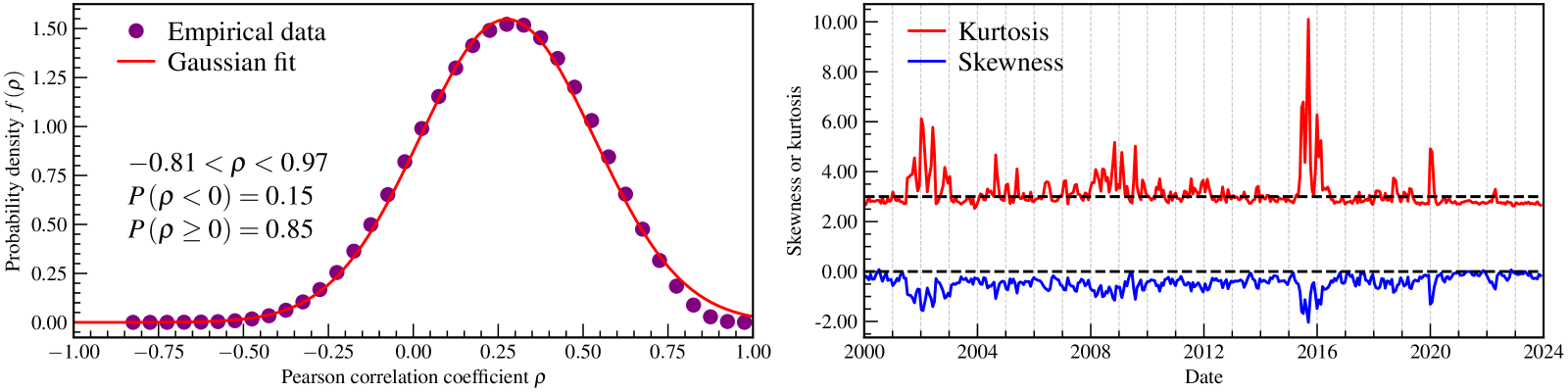
Figure 1: The distribution properties of the correlation coefficients. The left panel presents the estimated probability density function $f\left(\rho\right)$ of the correlation coefficients $\rho$ in the last time window. In this panel, the circles are data points, and the red curve is a Gaussian fit to the data points using non-linear least squares. The range of $\rho$ and the probabilities of $\rho<0$ and $\rho\geq 0$ are also shown in this panel. In the right panel, the kurtosis (upper red curve) and skewness (lower blue curve) of the correlation coefficients are plotted at the locations of the start dates of each time window. Both horizontal dashed straight lines indicate the locations of 3 and 0, which are the kurtosis and skewness of the Gaussian distribution, respectively.

To have an intuitive understanding of antinetwork structure, Fig. 2 shows a visualization of the antinetwork in the time window through Aug. 5, 2008 to Sept. 9, 2008, during which period the 2007–2008 global financial crisis was happening. This figure demonstrates that this antinetwork has a few huge and critical nodes. However, a similar structure is not observed in the corresponding network which is not visualized here because it has too many edges to make a legible picture. This difference in visualizations between antinetwork and network indicates that the node’s strength distributions for antinetwork and network follow different patterns.

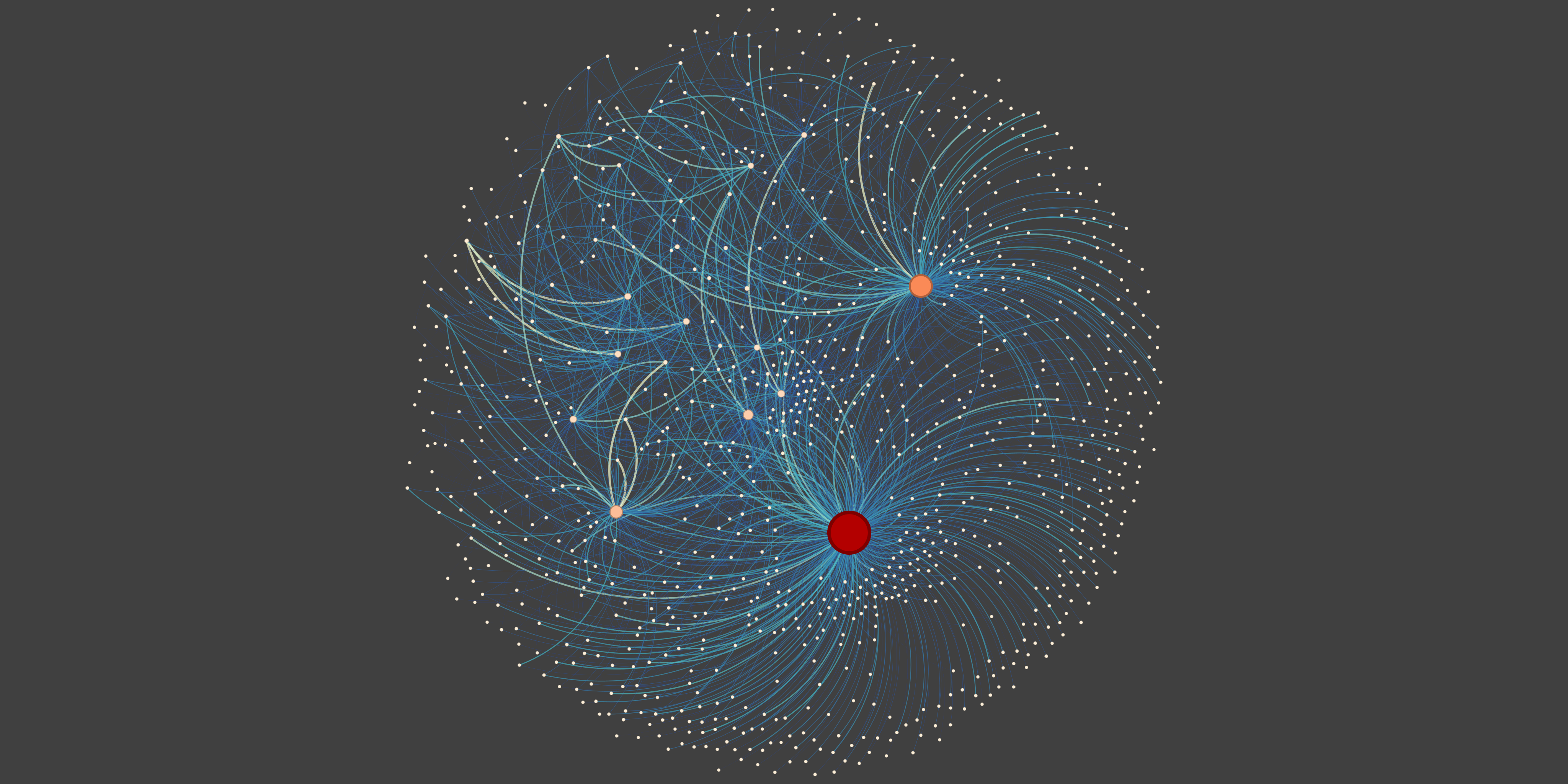
Figure 2: The visualization of a typical antinetwork with 994 nodes and 2,300 edges. This antinetwork is in the time window through Aug. 5, 2008 to Sept. 9, 2008, during which period the 2007–2008 global financial crisis was happening. A colored circle (node) represents a stock, whose color and size depend on its strength. A colored curve (edge) represents the correlation relationship between a pair of stocks linked by that curve, whose color and thickness depend on the correlation coefficient.

Fig. 3 presents both degree and strength distributions for the (anti)network in the last time window. It shows that the empirical distributions of both degree and strength for the antinetwork follow heavy-tailed distributions. This observation is further demonstrated by the power-law fits using non-linear least squares. Such heavy-tailed distributions have been observed in many complex networks [14, 16, 18, 28, 30, 44]. However, it is curious that these distributions for the network presented here do not show the heavy-tailed behavior.

This paper further examines these distributions for networks in all time windows, and observes that these distributions have similar shapes. To quantitatively examine the tail shapes of these distributions for antinetworks in all time windows, this paper employs the Generalized Pareto Distribution (GPD) to fit tail data and then to estimate the shape parameter $k$ by maximum likelihood estimation. The GPD is widely used to estimate the tail’s shape parameter $k$ because it includes both cases of the thin and heavy-tailed[39, 45, 46, 47]. The estimations with a threshold of 40% for antinetworks are presented in Fig. 4. It shows that the shape parameters $k$ for almost all antinetworks are positive and smaller than 1. A positive $k$ indicates a heavy-tailed distribution.

From the above studies, this paper finds that almost all antinetworks are scale-free in terms of degree and strength, while networks are not. This finding is in agreement with the observation of huge and critical nodes shown in Fig. 2. This difference between antinetwork and network has a crucial role in understanding the dynamics of a stock market.

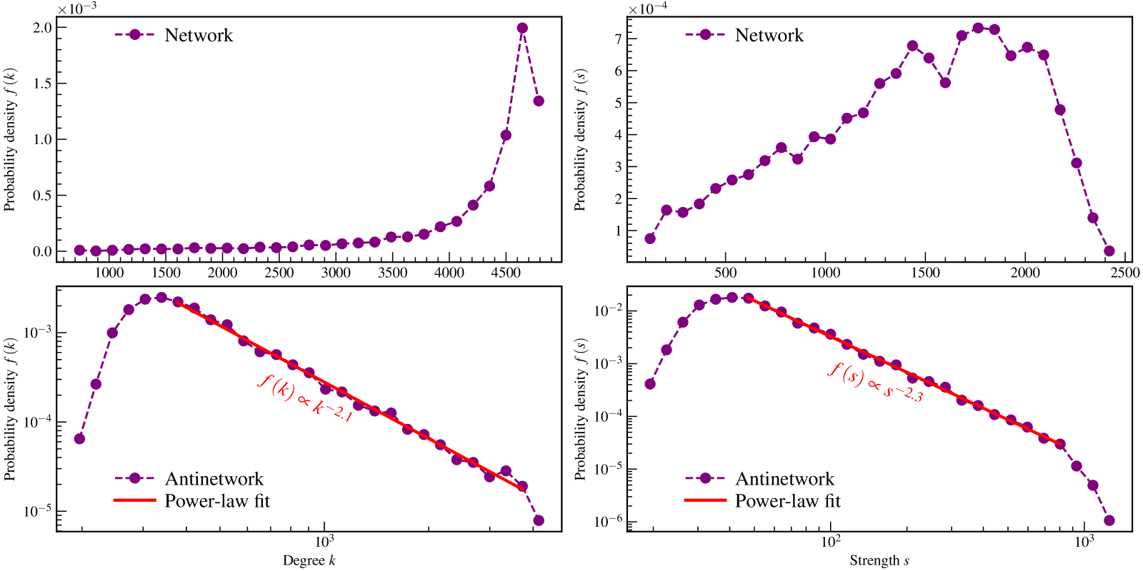
Figure 3: The probability density functions of both degree and strength for network and antinetwork. The upper and lower panels are for the network and antinetwork in the last time window, respectively. The solid purple circles are the estimated probability density functions of degree $k$ (left panels) and strength $s$ (right panels). The two solid red straight lines denote the results of the power-law fits to data points using non-linear least squares.

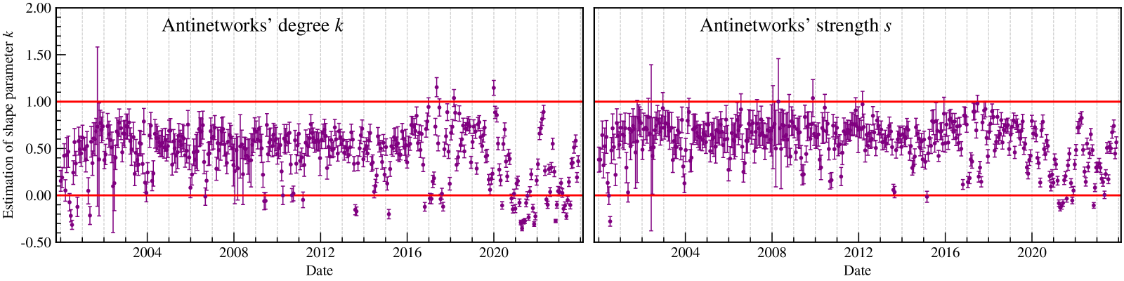
Figure 4: The estimations of the shape parameters of both degree and strength distributions for antinetworks. The left and right panels are for degree $k$ and strength $s$, respectively. The shape parameters are estimated from the GPD fit to the tail data over the threshold of 40th by maximum likelihood estimation. The purple circles are the point estimations, and the vertical purple lines with caps denote the 95% confidence intervals. The markers are plotted at the locations of the start dates of each time window. For ease of comparison, the locations of 0 and 1 are also denoted by the horizontal red straight lines.

Fig. 5 presents the assortativity coefficients $r$ by both degree and strength for networks and antinetworks. The coefficients of networks are close to 0. For the majority of networks, the coefficients by degree are positive, but the coefficients by strength are negative. Differently, all antinetworks behave significantly disassortative mixing by both degree and strength. This finding is in agreement with the visualization shown in Fig. 2. Compared with networks, the feature of assortative mixing for antinetworks is more sensitive to market crashes.

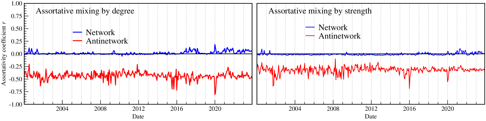
Figure 5: The assortativity coefficients by both degree and strength for networks and antinetworks. The left and right panels are for degree $k$ and strength $s$, respectively. The blue and red curves show the assortativity coefficients of networks and antinetworks, respectively. The curves are plotted at the locations of the start dates of each time window. For ease of comparison, the location of 0 is shown by the horizontal black straight lines.

Fig. 6 presents the average local clustering coefficients $\left<C\right>$ for networks and antinetworks. It clearly shows that the coefficients $\left<C\right>$ for networks are significantly larger than that for antinetworks. The extremely small coefficients $\left<C\right>$ indicate that a lot of star-like structures exist in antinetworks. The star-like structures are also observed in the visualization of the antinetwork shown in Fig. 2. Fig. 6 also shows that the market crashes may have opposite effects on $\left<C\right>$ for networks and antinetworks.

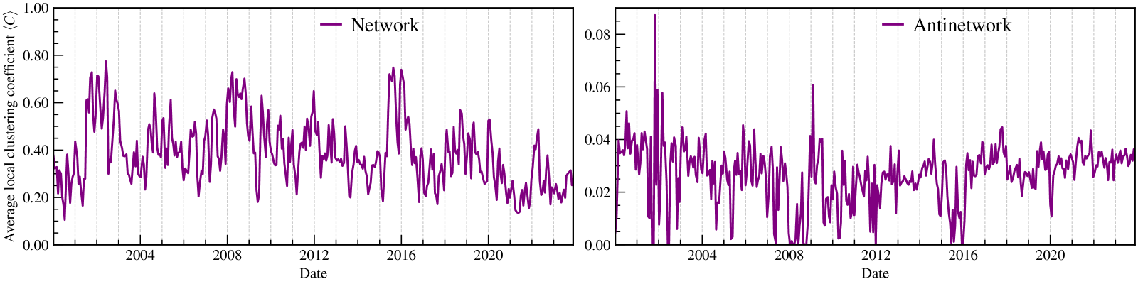
Figure 6: The average local clustering coefficients for networks and antinetworks. The left and right panels are for networks and antinetworks, respectively. The curves are plotted at the locations of the start dates of each time window.

Fig. 7 presents the average shortest path lengths $\left<L\right>$ for networks and antinetworks. It shows that the average shortest path lengths $\left<L\right>$ for networks are smaller than that for antinetworks. This figure also demonstrates that the market crashes have opposite effects on $\left<L\right>$ for networks and antinetworks. In the time windows when market crashes happen, $\left<L\right>$ significantly decreases and increases for networks and antinetworks, respectively. These significant changes in $\left<L\right>$ may be caused by the synchronization of the fluctuations of stock prices during periods of market crashes.

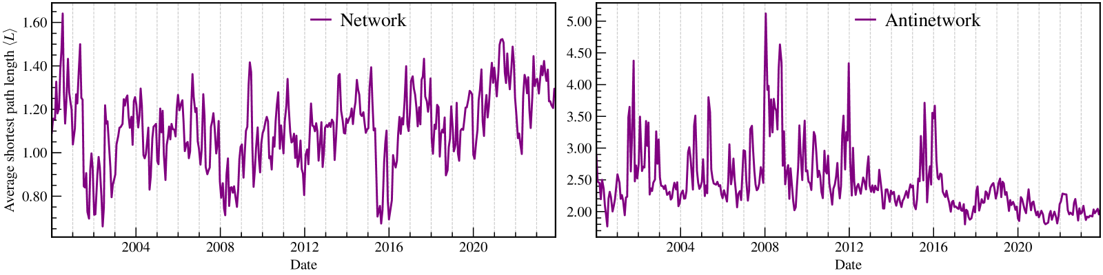
Figure 7: The average shortest path lengths for networks and antinetworks. The left and right panels are for networks and antinetworks, respectively. The curves are plotted at the locations of the start dates of each time window.

According to the discussion based on the measurements presented in Figs. 5, 6, and 7, stock market crashes impact these measurements significantly. To quantitatively investigate the effect of stock market fluctuations, this paper studies the relationships between these measurements and the return $R^{\prime}$ of the Shanghai Securities Composite Index. The return $R^{\prime}$ in the $m$th time window is defined as $R^{\prime}=\ln C_{m}-\ln O_{m}$, where $C_{m}$ and $O_{m}$ are the closure and open indices of the Shanghai Securities Composite Index in the $m$th time window, respectively. Fig. 8 shows the functions of the assortativity coefficient $r$ by strength, the average local clustering coefficient $\left<C\right>$, and the average shortest path length $\left<L\right>$ with respect to the return $R^{\prime}$.

Based on the data presented in Fig. 8, the following findings are concluded. Firstly, the stock market decline has no significant effect on the assortativity coefficient $r$ by strength for network. However, the market crash seems to decrease that for antinetwork. Secondly, during the time of the stock market decline ($R^{\prime}<0$), the average local clustering coefficient $\left<C\right>$ for network is a monotonic decreasing function of return $R^{\prime}$, while $\left<C\right>$ for antinetwork is a monotonic increasing function. Thirdly, when $R^{\prime}<0$, the average shortest path length $\left<L\right>$ for network is a monotonic increasing function of return $R^{\prime}$, while $\left<L\right>$ for antinetwork is a monotonic decreasing function. Lastly but surprisingly, the stock market rise ($R^{\prime}>0$) has no significant effects on these three measurements for both antinetwork and network.

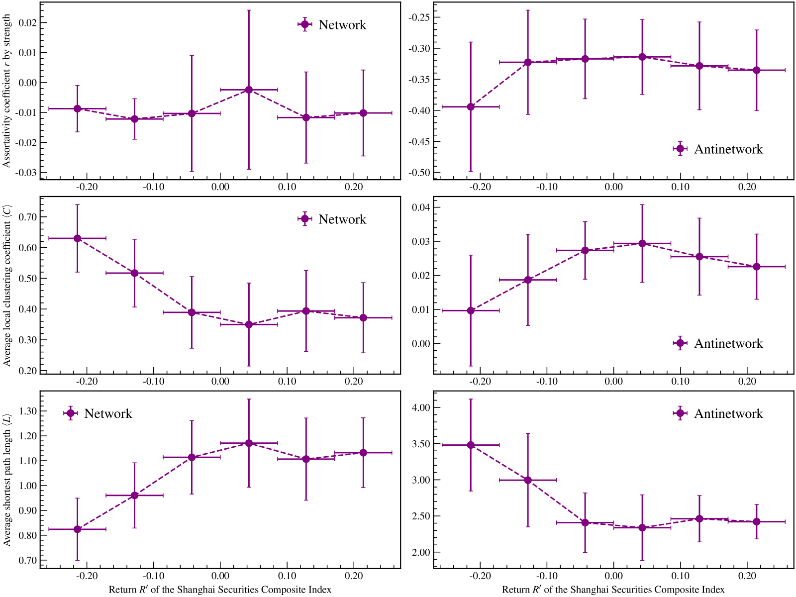
Figure 8: The assortativity coefficient, the average local clustering coefficient, and the average shortest path length as functions of the return of the Shanghai Securities Composite Index. The left and right panels are for network and antinetwork, respectively. The upper, middle, and lower panels present the assortativity coefficient $r$ by strength, the average local clustering coefficient $\left<C\right>$, and the average shortest path length $\left<L\right>$, respectively. The circles represent mean values in the specific ranges of return as shown by the horizontal lines with caps. The vertical lines with caps are the standard deviations.

5 Conclusions

The correlation-based financial networks, constructed with the correlation relationships among the time series of fluctuations of daily logarithmic prices of stocks, are intensively studied. However, these studies ignore the importance of negative correlations. Compared with the positive correlation, the negative correlation plays a more important role in understanding specific properties of a financial complex system. For example, the negative correlation can diversify market risk, and it consequently plays a crucial role in optimizing investment portfolios and risk management.

To pay attention to the negative correlations, this paper is the first time to consider the negative and positive correlations separately, and accordingly to construct weighted antinetwork and network based on the negative and positive correlation coefficients among the daily logarithmic returns of 5,329 stocks listed in the Shanghai and Shenzhen stock exchanges. To investigate the temporal evolution characteristics of (anti)network, this paper uses the technique of sliding time window and then constructs 387 (anti)networks during the 24 years from Jan. 1, 2000 to Dec. 31, 2023.

This work focuses on the differences in topological structures between antinetwork and network, and systematically analyzes the most fundamental (anti)network topological measurements: the node’s degree and strength, the assortativity coefficient, the average local clustering coefficient, and the average shortest path length. This paper finds some essential differences between antinetwork and network and concludes these findings as follows. (1) Almost all antinetworks are scale-free in terms of both degree and strength, while networks are not. (2) The antinetworks behave significantly disassortative mixing by both degree and strength, while the assortativity coefficients of networks are close to 0; the average local clustering coefficients for antinetworks are significantly smaller than that for networks; the average shortest path lengths for antinetworks are larger than that for networks. (3) The stock market crash seems to decrease antinetwork’s assortativity coefficient, while the stock market decline has no significant effect on network’s assortative mixing behavior; the stock market decline has opposite effects on antinetwork and network in terms of both the average local clustering coefficient and the average shortest path length; the stock market rise has no significant effects on these three topological measurements for both antinetwork and network.

The findings of the differences between antinetwork and network have an important role in understanding the dynamics of a financial complex system. The observation of antinetwork is of great importance in optimizing investment portfolios and risk management. More importantly, this paper proposes a new direction for studying complex systems, namely the correlation-based antinetwork.

CRediT authorship contribution statement

Peng Liu: Conceptualization, Resources, Data curation, Software, Formal Analysis, Funding acquisition, Validation, Investigation, Visualization, Methodology, Writing – original draft, Writing – review & editing.

Funding

This work was supported by the Humanities and Social Sciences Youth Foundation of the Ministry of Education of China [grant number 22YJCZH107]; the Shaanxi Science and Technology Department, P.R. China [grant number 2023-JC-QN-0093].

Declaration of competing interest

The authors declare that they have no known competing financial interests or personal relationships that could have appeared to influence the work reported in this paper.

Data availability

All raw data for this study were crawled from the Eastmoney website (https://quote.eastmoney.com). These data are publicly available on the Eastmoney website or from the corresponding author upon reasonable request.

References

- [1] Gupta, S., Mastrantonas, N., Masoller, C. & Kurths, J. Perspectives on the importance of complex systems in understanding our climate and climate change—The Nobel Prize in Physics 2021. attr/Border[0 0 0 [1 5] ]/H/I/C[0 1 1]user/Subtype/Link/A¡¡/Type/Action/S/URI/URI(https://doi.org/10.1063/5.0090222)¿¿Chaos 32, 052102 (2022).
- [2] Bianconi, G. et al. Complex systems in the spotlight: next steps after the 2021 Nobel Prize in Physics. attr/Border[0 0 0 [1 5] ]/H/I/C[0 1 1]user/Subtype/Link/A¡¡/Type/Action/S/URI/URI(https://doi.org/10.1088/2632-072X/ac7f75)¿¿J. Phys. Complex. 4, 010201 (2023).
- [3] Watts, D. J. & Strogatz, S. H. Collective dynamics of ‘small-world’networks. attr/Border[0 0 0 [1 5] ]/H/I/C[0 1 1]user/Subtype/Link/A¡¡/Type/Action/S/URI/URI(https://doi.org/10.1038/30918)¿¿Nature 393, 440–442 (1998).
- [4] Garlaschelli, D., Caldarelli, G. & Pietronero, L. Universal scaling relations in food webs. attr/Border[0 0 0 [1 5] ]/H/I/C[0 1 1]user/Subtype/Link/A¡¡/Type/Action/S/URI/URI(https://doi.org/10.1038/nature01604)¿¿Nature 423, 165–168 (2003).
- [5] Buldyrev, S. V., Parshani, R., Paul, G., Stanley, H. E. & Havlin, S. Catastrophic cascade of failures in interdependent networks. attr/Border[0 0 0 [1 5] ]/H/I/C[0 1 1]user/Subtype/Link/A¡¡/Type/Action/S/URI/URI(https://doi.org/10.1038/nature08932)¿¿Nature 464, 1025–1028 (2010).
- [6] Barabási, A.-L., Gulbahce, N. & Loscalzo, J. Network medicine: a network-based approach to human disease. attr/Border[0 0 0 [1 5] ]/H/I/C[0 1 1]user/Subtype/Link/A¡¡/Type/Action/S/URI/URI(https://doi.org/10.1038/nrg2918)¿¿Nat. Rev. Genet. 12, 56–68 (2011).
- [7] Oh, S. W. et al. A mesoscale connectome of the mouse brain. attr/Border[0 0 0 [1 5] ]/H/I/C[0 1 1]user/Subtype/Link/A¡¡/Type/Action/S/URI/URI(https://doi.org/10.1038/nature13186)¿¿Nature 508, 207–214 (2014).
- [8] Pilosof, S., Porter, M. A., Pascual, M. & Kéfi, S. The multilayer nature of ecological networks. attr/Border[0 0 0 [1 5] ]/H/I/C[0 1 1]user/Subtype/Link/A¡¡/Type/Action/S/URI/URI(https://doi.org/10.1038/s41559-017-0101)¿¿Nat. Ecol. Evol. 1, 0101 (2017).
- [9] Liu, H., Han, D., Ma, Y. & Zhu, L. Network structure of thermonuclear reactions in nuclear landscape. attr/Border[0 0 0 [1 5] ]/H/I/C[0 1 1]user/Subtype/Link/A¡¡/Type/Action/S/URI/URI(https://doi.org/10.1007/s11433-020-1552-2)¿¿Sci. China Phys. Mech. Astron. 63, 112062 (2020).
- [10] Bardoscia, M. et al. The physics of financial networks. attr/Border[0 0 0 [1 5] ]/H/I/C[0 1 1]user/Subtype/Link/A¡¡/Type/Action/S/URI/URI(https://doi.org/10.1038/s42254-021-00322-5)¿¿Nat. Rev. Phys. 3, 490–507 (2021).
- [11] Jusup, M. et al. Social physics. attr/Border[0 0 0 [1 5] ]/H/I/C[0 1 1]user/Subtype/Link/A¡¡/Type/Action/S/URI/URI(https://doi.org/10.1016/j.physrep.2021.10.005)¿¿Phys. Rep. 948, 1–148 (2022).
- [12] Kuhlmann, M. Explaining financial markets in terms of complex systems. attr/Border[0 0 0 [1 5] ]/H/I/C[0 1 1]user/Subtype/Link/A¡¡/Type/Action/S/URI/URI(https://doi.org/10.1086/677699)¿¿Philos. Sci. 81, 1117––1130 (2014).
- [13] Mantegna, R. N. Hierarchical structure in financial markets. attr/Border[0 0 0 [1 5] ]/H/I/C[0 1 1]user/Subtype/Link/A¡¡/Type/Action/S/URI/URI(https://doi.org/10.1007/s100510050929)¿¿Eur. Phys. J. B 11, 193–197 (1999).
- [14] Bonanno, G., Caldarelli, G., Lillo, F. & Mantegna, R. N. Topology of correlation-based minimal spanning trees in real and model markets. attr/Border[0 0 0 [1 5] ]/H/I/C[0 1 1]user/Subtype/Link/A¡¡/Type/Action/S/URI/URI(https://doi.org/10.1103/PhysRevE.68.046130)¿¿Phys. Rev. E 68, 046130 (2003).
- [15] Onnela, J.-P., Chakraborti, A., Kaski, K. & Kertész, J. Dynamic asset trees and Black Monday. attr/Border[0 0 0 [1 5] ]/H/I/C[0 1 1]user/Subtype/Link/A¡¡/Type/Action/S/URI/URI(https://doi.org/10.1016/S0378-4371(02)01882-4)¿¿Physica A 324, 247–252 (2003).
- [16] Onnela, J.-P., Chakraborti, A., Kaski, K., Kertész, J. & Kanto, A. Dynamics of market correlations: Taxonomy and portfolio analysis. attr/Border[0 0 0 [1 5] ]/H/I/C[0 1 1]user/Subtype/Link/A¡¡/Type/Action/S/URI/URI(https://doi.org/10.1103/PhysRevE.68.056110)¿¿Phys. Rev. E 68, 056110 (2003).
- [17] Lee, J., Youn, J. & Chang, W. Intraday volatility and network topological properties in the Korean stock market. attr/Border[0 0 0 [1 5] ]/H/I/C[0 1 1]user/Subtype/Link/A¡¡/Type/Action/S/URI/URI(https://doi.org/10.1016/j.physa.2011.09.016)¿¿Physica A 391, 1354–1360 (2012).
- [18] Wiliński, M., Sienkiewicz, A., Gubiec, T., Kutner, R. & Struzik, Z. Structural and topological phase transitions on the German Stock Exchange. attr/Border[0 0 0 [1 5] ]/H/I/C[0 1 1]user/Subtype/Link/A¡¡/Type/Action/S/URI/URI(https://doi.org/10.1016/j.physa.2013.07.064)¿¿Physica A 392, 5963–5973 (2013).
- [19] Huang, W.-Q., Yao, S., Zhuang, X.-T. & Yuan, Y. Dynamic asset trees in the US stock market: Structure variation and market phenomena. attr/Border[0 0 0 [1 5] ]/H/I/C[0 1 1]user/Subtype/Link/A¡¡/Type/Action/S/URI/URI(https://doi.org/10.1016/j.chaos.2016.11.007)¿¿Chaos Solitons Fractals 94, 44–53 (2017).
- [20] Nguyen, Q., Nguyen, N. K. & Nguyen, L. N. Dynamic topology and allometric scaling behavior on the Vietnamese stock market. attr/Border[0 0 0 [1 5] ]/H/I/C[0 1 1]user/Subtype/Link/A¡¡/Type/Action/S/URI/URI(https://doi.org/10.1016/j.physa.2018.09.061)¿¿Physica A 514, 235–243 (2019).
- [21] Huang, C., Zhao, X., Su, R., Yang, X. & Yang, X. Dynamic network topology and market performance: A case of the Chinese stock market. attr/Border[0 0 0 [1 5] ]/H/I/C[0 1 1]user/Subtype/Link/A¡¡/Type/Action/S/URI/URI(https://doi.org/10.1002/ijfe.2253)¿¿Int. J. Finance Econ. 27, 1962–1978 (2022).
- [22] Tumminello, M., Aste, T., Matteo, T. D. & Mantegna, R. N. A tool for filtering information in complex systems. attr/Border[0 0 0 [1 5] ]/H/I/C[0 1 1]user/Subtype/Link/A¡¡/Type/Action/S/URI/URI(https://doi.org/10.1073/pnas.0500298102)¿¿Proc. Natl. Acad. Sci. USA 102, 10421–10426 (2005).
- [23] Tumminello, M., Di Matteo, T., Aste, T. & Mantegna, R. N. Correlation based networks of equity returns sampled at different time horizons. attr/Border[0 0 0 [1 5] ]/H/I/C[0 1 1]user/Subtype/Link/A¡¡/Type/Action/S/URI/URI(https://doi.org/10.1140/epjb/e2006-00414-4)¿¿Eur. Phys. J. B 55, 209–217 (2007).
- [24] Vodenska, I. et al. Community analysis of global financial markets. attr/Border[0 0 0 [1 5] ]/H/I/C[0 1 1]user/Subtype/Link/A¡¡/Type/Action/S/URI/URI(https://doi.org/10.3390/risks4020013)¿¿Risks 4, 13 (2016).
- [25] Zhao, L. et al. Stock market as temporal network. attr/Border[0 0 0 [1 5] ]/H/I/C[0 1 1]user/Subtype/Link/A¡¡/Type/Action/S/URI/URI(https://doi.org/10.1016/j.physa.2018.05.039)¿¿Physica A 506, 1104–1112 (2018).
- [26] Onnela, J. P., Kaski, K. & Kertész, J. Clustering and information in correlation based financial networks. attr/Border[0 0 0 [1 5] ]/H/I/C[0 1 1]user/Subtype/Link/A¡¡/Type/Action/S/URI/URI(https://doi.org/10.1140/epjb/e2004-00128-7)¿¿Eur. Phys. J. B 38, 353–362 (2004).
- [27] Onnela, J.-P., Saramäki, J., Kertész, J. & Kaski, K. Intensity and coherence of motifs in weighted complex networks. attr/Border[0 0 0 [1 5] ]/H/I/C[0 1 1]user/Subtype/Link/A¡¡/Type/Action/S/URI/URI(https://doi.org/10.1103/PhysRevE.71.065103)¿¿Phys. Rev. E 71, 065103(R) (2005).
- [28] Huang, W.-Q., Zhuang, X.-T. & Yao, S. A network analysis of the Chinese stock market. attr/Border[0 0 0 [1 5] ]/H/I/C[0 1 1]user/Subtype/Link/A¡¡/Type/Action/S/URI/URI(https://doi.org/10.1016/j.physa.2009.03.028)¿¿Physica A 388, 2956–2964 (2009).
- [29] Xi, X. & An, H. Research on energy stock market associated network structure based on financial indicators. attr/Border[0 0 0 [1 5] ]/H/I/C[0 1 1]user/Subtype/Link/A¡¡/Type/Action/S/URI/URI(https://doi.org/10.1016/j.physa.2017.08.114)¿¿Physica A 490, 1309–1323 (2018).
- [30] Xia, L., You, D., Jiang, X. & Guo, Q. Comparison between global financial crisis and local stock disaster on top of Chinese stock network. attr/Border[0 0 0 [1 5] ]/H/I/C[0 1 1]user/Subtype/Link/A¡¡/Type/Action/S/URI/URI(https://doi.org/10.1016/j.physa.2017.08.005)¿¿Physica A 490, 222–230 (2018).
- [31] So, M. K., Chu, A. M. & Chan, T. W. Impacts of the COVID-19 pandemic on financial market connectedness. attr/Border[0 0 0 [1 5] ]/H/I/C[0 1 1]user/Subtype/Link/A¡¡/Type/Action/S/URI/URI(https://doi.org/10.1016/j.frl.2020.101864)¿¿Finance Res. Lett. 38, 101864 (2021).
- [32] Peron, T., Costa, L. & Rodrigues, F. A. The structure and resilience of financial market networks. attr/Border[0 0 0 [1 5] ]/H/I/C[0 1 1]user/Subtype/Link/A¡¡/Type/Action/S/URI/URI(https://doi.org/10.1063/1.3683467)¿¿Chaos 22, 013117 (2012).
- [33] Li, S., He, J. & Song, K. Network entropies of the Chinese financial market. attr/Border[0 0 0 [1 5] ]/H/I/C[0 1 1]user/Subtype/Link/A¡¡/Type/Action/S/URI/URI(https://doi.org/10.3390/e18090331)¿¿Entropy 18, 331 (2016).
- [34] Pan, Z., Ma, Q., Ding, J. & Wang, L. Research on the stock correlation networks and network entropies in the Chinese green financial market. attr/Border[0 0 0 [1 5] ]/H/I/C[0 1 1]user/Subtype/Link/A¡¡/Type/Action/S/URI/URI(https://doi.org/10.1140/epjb/s10051-021-00063-5)¿¿Eur. Phys. J. B 94, 56 (2021).
- [35] Liu, W., Ma, Q. & Liu, X. Research on the dynamic evolution and its influencing factors of stock correlation network in the Chinese new energy market. attr/Border[0 0 0 [1 5] ]/H/I/C[0 1 1]user/Subtype/Link/A¡¡/Type/Action/S/URI/URI(https://doi.org/10.1016/j.frl.2021.102138)¿¿Finance Res. Lett. 45, 102138 (2022).
- [36] The STAR Collaboration. Observation of an antimatter hypernucleus. attr/Border[0 0 0 [1 5] ]/H/I/C[0 1 1]user/Subtype/Link/A¡¡/Type/Action/S/URI/URI(https://doi.org/10.1126/science.1183980)¿¿Science 328, 58–62 (2010).
- [37] The STAR Collaboration. Measurement of the mass difference and the binding energy of the hypertriton and antihypertriton. attr/Border[0 0 0 [1 5] ]/H/I/C[0 1 1]user/Subtype/Link/A¡¡/Type/Action/S/URI/URI(https://doi.org/10.1038/s41567-020-0799-7)¿¿Nat. Phys. 16, 409–412 (2020).
- [38] Liu, P. & Zheng, Y. Temporal and spatial evolution of the distribution related to the number of COVID-19 pandemic. attr/Border[0 0 0 [1 5] ]/H/I/C[0 1 1]user/Subtype/Link/A¡¡/Type/Action/S/URI/URI(https://doi.org/10.1016/j.physa.2022.127837)¿¿Physica A 603, 127837 (2022).
- [39] Liu, P. & Zheng, Y. Heavy-tailed distributions of confirmed COVID-19 cases and deaths in spatiotemporal space. attr/Border[0 0 0 [1 5] ]/H/I/C[0 1 1]user/Subtype/Link/A¡¡/Type/Action/S/URI/URI(https://doi.org/10.1371/journal.pone.0294445)¿¿PLOS ONE 18, e0294445 (2023).
- [40] Liu, P. & Zheng, Y. Precision measurement of the return distribution property of the Chinese stock market index. attr/Border[0 0 0 [1 5] ]/H/I/C[0 1 1]user/Subtype/Link/A¡¡/Type/Action/S/URI/URI(https://doi.org/10.3390/e25010036)¿¿Entropy 25, 36 (2023).
- [41] Opsahl, T., Agneessens, F. & Skvoretz, J. Node centrality in weighted networks: Generalizing degree and shortest paths. attr/Border[0 0 0 [1 5] ]/H/I/C[0 1 1]user/Subtype/Link/A¡¡/Type/Action/S/URI/URI(https://doi.org/10.1016/j.socnet.2010.03.006)¿¿Social Networks 32, 245–251 (2010).
- [42] Newman, M. E. J. Assortative mixing in networks. attr/Border[0 0 0 [1 5] ]/H/I/C[0 1 1]user/Subtype/Link/A¡¡/Type/Action/S/URI/URI(https://doi.org/PhysRevLett.89.208701)¿¿Phys. Rev. Lett. 89, 208701 (2002).
- [43] Newman, M. E. J. Networks (Oxford University Press, Oxford, 2018), 2nd edn.
- [44] Barabási, A.-L. & Albert, R. Emergence of scaling in random networks. attr/Border[0 0 0 [1 5] ]/H/I/C[0 1 1]user/Subtype/Link/A¡¡/Type/Action/S/URI/URI(https://doi.org/10.1126/science.286.5439.509)¿¿Science 286, 509–512 (1999).
- [45] Conte, M. N. & Kelly, D. L. An imperfect storm: Fat-tailed tropical cyclone damages, insurance, and climate policy. attr/Border[0 0 0 [1 5] ]/H/I/C[0 1 1]user/Subtype/Link/A¡¡/Type/Action/S/URI/URI(https://doi.org/10.1016/j.jeem.2017.08.010)¿¿J. Environ. Econ. Manag. 92, 677–706 (2018).
- [46] Embrechts, P., Klüppelberg, C. & Mikosch, T. Modelling Extremal Events for Insurance and Finance (Springer, New York, 1997).
- [47] Kotz, S. & Nadarajah, S. Extreme Value Distributions: Theory and Applications (Imperial College Press, London, 2000).