Technical Report: Pose Graph Optimization over Planar Unit Dual Quaternions: Improved Accuracy with Provably Convergent Riemannian Optimization

Abstract

It is common in pose graph optimization (PGO) algorithms to assume that noise in the translations and rotations of relative pose measurements is uncorrelated. However, existing work shows that in practice these measurements can be highly correlated, which leads to degradation in the accuracy of PGO solutions that rely on this assumption. Therefore, in this paper we develop a novel algorithm derived from a realistic, correlated model of relative pose uncertainty, and we quantify the resulting improvement in the accuracy of the solutions we obtain relative to state-of-the-art PGO algorithms. Our approach utilizes Riemannian optimization on the planar unit dual quaternion (PUDQ) manifold, and we prove that it converges to first-order stationary points of a Lie-theoretic maximum likelihood objective. Then we show experimentally that, compared to state-of-the-art PGO algorithms, this algorithm produces estimation errors that are lower by 10% to 25% across several orders of magnitude of noise levels and graph sizes.

I Introduction

Pose graph optimization (PGO) algorithms aim to optimally reconstruct the trajectory of a mobile agent using a set of uncertain relative measurements that were collected over time. PGO is a backend component for numerous applications in robotics and computer vision, including simultaneous localization and mapping (SLAM) [1, 2], bundle adjustment [3], structure from motion [4], and photogrammetry [5]. Additionally, the PGO framework readily accommodates a variety of practical problems of interest [6, 7, 8, 9], making it a versatile tool for optimization in robotics and computer vision.

Some well-established PGO frameworks, such as g2o [10], GTSAM [11], and iSAM [12], have addressed the PGO problem using a mix of Euclidean and heuristic optimization techniques. More recently, algorithms based on Riemannian optimization, including SE-Sync [13], Cartan-Sync [14], and CPL-Sync [15], have demonstrated that, under certain conditions, the PGO problem admits a semidefinite relaxation whose solution approximates the solution of the original, unrelaxed problem. One condition assumed by the above algorithms (and others) is that uncertainties in a mobile agent’s position and orientation are modeled by isotropic noise.

However, the isotropic noise assumption runs contrary to existing results on uncertainty representations for rigid motion groups, which mathematically encode PGO problems. Specifically, it was shown in 2D [16] and in 3D [17] that the propagation of uncertainty through compound, rigid motions is best captured by a Lie-theoretic model [18], namely, a Gaussian distribution on the Lie algebra of a rigid motion group. In fact, the authors of [19] demonstrated that such a Lie-theoretic model accurately predicted the distribution of a compound rigid motion trajectory where traditional models failed. These Lie-theoretic models are inherently anisotropic, which suggests that a PGO algorithm that incorporates anisotropy may attain improved accuracy.

Therefore, in this paper, we formulate 2D PGO problems on the manifold of planar unit dual quaternions (PUDQs), which we use to explicitly incorporate anisotropy in uncertainty models. To solve such problems, we use a Riemannian trust region (RTR) algorithm, for which we derive global convergence guarantees. Overall, the contributions of this paper are:

• We present what is, to the best of our knowledge, the first provably convergent PGO algorithm that permits arbitrarily large, anisotropic uncertainties.

• We prove that the proposed algorithm converges to first-order critical points given any initialization.

• We show that the resulting pose estimates are always at least $10$% more accurate than the state of the art and more than $25$% more accurate on high-dimensional problems.

The closest related works are [20, 21, 22]. In [20], a unit dual quaternion approach to PGO was developed using heuristic optimization techniques without formal guarantees, whereas we employ theoretically grounded, provably convergent Riemannian-geometric techniques. The authors of [21] used a Lie-theoretic objective, but did not include convergence guarantees or quantify the accuracy of their solutions. The work in [22] uses a similar problem formulation to us, though that work was entirely empirical. We differ both by proving convergence and showing improvement in accuracy over a class of Riemannian algorithms that were not studied in [22].

The rest of the paper is organized as follows. Section II provides preliminaries, and Section III provides a formal problem statement. Section IV outlines the proposed algorithm, and Section V proves that it converges. Section VI contains numerical results, and Section VII concludes.

II Preliminaries

In this section, we include mathematical preliminaries that are necessary for our PUDQ PGO problem formulation. For detailed derivations, see Appendices A-B.

II-A Planar unit dual quaternion construction

We construct the PUDQ manifold as a representation of planar rigid motion. Given an orthonormal basis $\{\mathbf{i},\mathbf{j},\mathbf{k}\}$, a planar rigid motion is characterized by a translation, denoted $\mathbf{t}=t_{x}\mathbf{i}+t_{y}\mathbf{j}$, and a rotation about the $\mathbf{k}$ axis by an angle $\theta\in(-\pi,\pi]$. The PUDQ parameterization of this motion is given by $\mathbf{x}=\mathbf{x}_{r}+\epsilon\mathbf{x}_{d}$, where $\epsilon$ is a dual number satisfying $\epsilon^{2}=0,\epsilon\neq 0$. The real and dual parts of $\mathbf{x}$, denoted $\mathbf{x}_{r}\in\mathbb{S}^{1}$ and $\mathbf{x}_{d}\in\mathbb{R}^{2}$, respectively, are $\mathbf{x}_{r}\triangleq\cos\left(\nicefrac{{\theta}}{{2}}\right)+\sin\left(\nicefrac{{\theta}}{{2}}\right)\mathbf{k}$ and $\mathbf{x}_{d}\triangleq\frac{1}{2}\boldsymbol{\mathrm{t}}\otimes\mathbf{x}_{r}$, with “$\otimes$” denoting the Hamilton product [23] under the convention $\mathbf{i}^{2}=\mathbf{j}^{2}=\mathbf{k}^{2}=\mathbf{i}\mathbf{j}\mathbf{k}=-1$. Applying the Hamilton product to two PUDQs, denoted $\mathbf{x}$ and $\mathbf{y}$, yields the composition operator “$\boxplus$”, which can be expressed as

$$\mathbf{x}\boxplus\mathbf{y}=\underset{Q_{L}\left(\mathbf{x}\right)}{\underbrace{\Bigg{[}\begin{smallmatrix}x_{0}&-x_{1}&0&0\\ x_{1}&x_{0}&0&0\\ x_{2}&x_{3}&x_{0}&-x_{1}\\ x_{3}&-x_{2}&x_{1}&x_{0}\end{smallmatrix}\Bigg{]}}}\underset{\mathbf{y}}{\underbrace{\Bigg{[}\begin{smallmatrix}y_{0}\\ y_{1}\\ y_{2}\\ y_{3}\end{smallmatrix}\Bigg{]}}}=\underset{Q_{R}\left(\mathbf{y}\right)}{\underbrace{\Bigg{[}\begin{smallmatrix}y_{0}&-y_{1}&0&0\\ y_{1}&y_{0}&0&0\\ y_{2}&-y_{3}&y_{0}&y_{1}\\ y_{3}&y_{2}&-y_{1}&y_{0}\end{smallmatrix}\Bigg{]}}}\underset{\mathbf{x}}{\underbrace{\Bigg{[}\begin{smallmatrix}x_{0}\\ x_{1}\\ x_{2}\\ x_{3}\end{smallmatrix}\Bigg{]}}},$$ (1)

where $Q_{L}(\cdot)$ and $Q_{R}(\cdot)$ denote the left and right composition maps, respectively. From (1), we have the identity element $\mathbbm{1}=\left[1,0,0,0\right]^{\top}$ and inverse formula $\mathbf{x}^{-1}=\left[x_{0},-x_{1},-x_{2},-x_{3}\right]^{\top}$. The set of PUDQs forms the smooth manifold $\mathcal{M}\triangleq\mathbb{S}^{1}\rtimes\mathbb{R}^{2}\subset\mathbb{R}^{4}$, which we embed in $\mathbb{R}^{4}$ as

$$\mathcal{M}\triangleq\left\{\mathbf{x}\in\mathbb{R}^{4}\mid h\left(\mathbf{x}\right)=\mathbf{x}^{\top}\tilde{P}\mathbf{x}-1=0\right\}\subset\mathbb{R}^{4},$$ (2)

where $\tilde{P}\triangleq\mathrm{diag}(\{1,1,0,0\})$ and $h(\mathbf{x})$ is the defining function [24] for $\mathcal{M}$. PGO algorithms optimize over $N$ poses, so we extend (2) to the $N$-fold product manifold $\mathcal{M}^{N}\triangleq(\mathbb{S}^{1}\rtimes\mathbb{R}^{2})^{N}$. Below, we will use the operator $\operatorname{vec}(\cdot)$, where $\operatorname{vec}((\mathbf{x}_{i})_{i=1}^{N})\triangleq[\mathbf{x}_{1}^{\top},\mathbf{x}_{2}^{\top},\dots,\mathbf{x}_{N}^{\top}]^{\top}$, with each $\mathbf{x}_{i}\in\mathcal{M}$. Since $(\mathbb{S}^{1}\rtimes\mathbb{R}^{2})^{N}\subset\mathbb{R}^{4\times N}\cong\mathbb{R}^{4N}$, we embed $\mathcal{M}^{N}$ in $\mathbb{R}^{4N}$. For $\mathcal{X},\mathcal{Y}\in\mathcal{M}^{N}$, this embedding lets us write $\mathcal{X}=\operatorname{vec}((\mathbf{x}_{i})_{i=1}^{N})$ and $\mathcal{Y}=\operatorname{vec}((\mathbf{y}_{i})_{i=1}^{N})$, where $\mathbf{x}_{i},\mathbf{y}_{i}\in\mathcal{M}$ for each $i$. This embedding also gives the identity $\mathbbm{1}^{N}=\operatorname{vec}((\mathbbm{1})_{i=1}^{N})$, the inverse formula $\mathcal{X}^{-1}=\operatorname{vec}((\mathbf{x}_{i}^{-1})_{i=1}^{N})$, and the product $\mathcal{X}\boxplus\mathcal{Y}=\operatorname{vec}\Big{(}(\mathbf{x}_{i}\boxplus\mathbf{y}_{i})_{i=1}^{N}\Big{)}$.

II-B Logarithm and exponential maps

The smooth manifold $\mathcal{M}$ with the identity, inverse, and composition operator form a Lie group[18] whose Lie algebra is the tangent space at the identity element, denoted $\mathcal{T}_{\mathbbm{1}}\mathcal{M}$. Given $\mathbf{x}\in\mathcal{M}$, the logarithm map at the identity element is $\textnormal{Log}_{\mathbbm{1}}:\mathcal{M}\rightarrow\mathcal{T}_{\mathbbm{1}}\mathcal{M}$, given by

$$\textnormal{Log}_{\mathbbm{1}}\!\left(\mathbf{x}\right)=\frac{1}{\gamma\left(\mathbf{x}\right)}{\left[x_{1},\leavevmode\nobreak\ x_{2},\leavevmode\nobreak\ x_{3}\right]}^{\top},$$ (3)

with $\gamma\left(\mathbf{x}\right)\triangleq\mathrm{sinc}\left(\phi\left(\mathbf{x}\right)\right)=\sin\left(\phi\left(\mathbf{x}\right)\right)/\phi\left(\mathbf{x}\right)$, where $\phi\left(\mathbf{x}\right)\triangleq\mathrm{wrap}\left(\mathrm{arctan}\left(x_{1},x_{0}\right)\right)$, $\operatorname{arctan}:\mathbb{S}^{1}\rightarrow(-\pi,\pi]$ is the four-quadrant arctangent and

$$\mathrm{wrap}\left(\alpha\right)\triangleq\begin{cases}\alpha+\pi&\text{if }\alpha\leq-\nicefrac{{\pi}}{{2}}\\ \alpha-\pi&\text{if }\alpha>\nicefrac{{\pi}}{{2}}\\ \alpha&\text{otherwise}.\end{cases}$$ (4)

Here, $\phi:\mathcal{M}\rightarrow\left(-\nicefrac{{\pi}}{{2}},\nicefrac{{\pi}}{{2}}\right]$ computes the half-angle of rotation about the $\mathbf{k}$-axis encoded by a point on $\mathcal{M}$. The half-angles $\phi+n\pi$ for all $n\in\mathbb{Z}$ encode the same rotation, so it is valid to wrap $\phi$ to $(-\nicefrac{{\pi}}{{2}},\nicefrac{{\pi}}{{2}}]$ via (4).

Given $\mathbf{x}_{t}=\left[x_{t,1},\leavevmode\nobreak\ x_{t,2},\leavevmode\nobreak\ x_{t,3}\right]^{\top}\in\mathcal{T}_{\mathbbm{1}}\mathcal{M}$, the exponential map at the identity, denoted $\mathrm{Exp}_{\mathbbm{1}}:T_{\mathbbm{1}}\mathcal{M}\rightarrow\mathcal{M}$, is given by $\textnormal{Exp}_{\mathbbm{1}}\!\left(\mathbf{x}_{t}\right)={\left[\cos\left(x_{t,1}\right),\gamma\left(\mathbf{x}_{t}\right)\mathbf{x}_{t}^{\top}\right]}^{\top}$, where $\gamma\left(\mathbf{x}_{t}\right)\triangleq\operatorname{sinc}\left(x_{t,1}\right)$ as above. For any $\mathbf{x},\boldsymbol{\mathrm{y}}\in\mathcal{M}$, we also have the point-wise logarithm map

$$\textnormal{Log}_{\mathbf{x}}\!\left(\mathbf{y}\right)=\mathbf{x}\boxplus[0,\textnormal{Log}_{\mathbbm{1}}\!(\mathbf{x}^{-1}\boxplus\mathbf{y})^{\top}]^{\top},$$ (5)

and, for $\mathbf{x}\in\mathcal{M},\boldsymbol{\mathrm{y}}_{t}\in\mathcal{T}_{\mathbf{x}}\mathcal{M}$, the point-wise exponential map

$$\textnormal{Exp}_{\mathbf{x}}\!\left(\mathbf{y}_{t}\right)=\mathbf{x}\boxplus\textnormal{Exp}_{\mathbbm{1}}\!\left(\left(\mathbf{x}^{-1}\boxplus\mathbf{y}_{t}\right)_{1:3}\right),$$ (6)

where ${\left(\cdot\right)}_{1:3}$ selects the last three entries of a vector. For $\mathcal{X},\mathcal{Y}\in\mathcal{M}^{N}$, (5)-(6) give logarithm and exponential maps over the product manifold $\mathcal{M}^{N}$, namely $\textnormal{Log}_{\mathcal{X}}\!\left(\mathcal{Y}\right)=\operatorname{vec}\left((\textnormal{Log}_{\mathbf{x}_{i}}(\mathbf{y}_{i}))_{i=1}^{N}\right)$, and, for any $\mathcal{Y}_{t}=\operatorname{vec}\left((\mathbf{y}_{t,i})_{i=1}^{N}\right)\in\mathcal{T}_{\mathcal{X}}\mathcal{M}^{N}$, the mapping

$$\textnormal{Exp}_{\mathcal{X}}\!\left(\mathcal{Y}_{t}\right)=\operatorname{vec}\left((\textnormal{Exp}_{\mathbf{x}_{i}}(\mathbf{y}_{t,i}))_{i=1}^{N}\right),$$ (7)

with $\textnormal{Log}_{\mathbf{x}_{i}}(\cdot)$ and $\textnormal{Exp}_{\mathbf{x}_{i}}(\cdot)$ given by (5) and (6).

II-C Pose Graph Construction

We now address the construction of a pose graph, as exemplified in Figure 1. First, let $\mathcal{G}=(\mathcal{V},\mathcal{E})$ be a directed graph with vertex set $\mathcal{V}$ and edge set $\mathcal{E}$ of ordered pairs $(i,j)\in\mathcal{V}\times\mathcal{V}$. Letting $|\mathcal{V}|=N$, we define $\mathcal{X}=\operatorname{vec}((\mathbf{x}_{i})_{i\in\mathcal{V}})\in\mathcal{M}^{N}$ to be the vector of $N$ poses to be estimated, with individual poses denoted $\mathbf{x}_{i}\in\mathcal{M}$. Then, letting $\left|\mathcal{E}\right|=M$, we define $\mathcal{Z}=\operatorname{vec}((\tilde{\mathbf{z}}_{ij})_{\left(i,j\right)\in\mathcal{E}})\in\mathcal{M}^{M}$ to be the vector of $M$ relative pose measurements, where $\tilde{\mathbf{z}}_{ij}\in\mathcal{M}$ encodes a measured transformation from $\mathbf{x}_{i}$ to $\mathbf{x}_{j}$, taken in the frame of $\mathbf{x}_{i}$. The noise covariance for $\tilde{\mathbf{z}}_{ij}$ is given by the matrix $\Sigma_{ij}$. The corresponding pose graph is then constructed by associating the vertex set $\mathcal{V}$ with $\mathcal{X}$, and the edge set $\mathcal{E}$ with $\mathcal{Z}$.

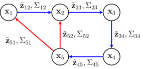
Figure 1: A pose graph with $N=M=5$, labeled with vertex poses $\mathbf{x}_{i}$, edge measurements $\tilde{\mathbf{z}}_{ij}$, and edge covariances $\Sigma_{ij}$. Odometry edges, shown in blue, connect neighboring vertices (i.e., $\left|j-i\right|=1$). Loop closure edges, shown in red, connect any non-neighboring vertices (i.e., $\left|j-i\right|>1$).

III Problem Formulation

We now derive the problem to be solved. From the perspective of Bayesian inference, PGO algorithms aim to estimate the posterior distribution of poses that best fits a given dataset of relative measurements made along a trajectory. Because a prior distribution is not always available, PGO is typically formulated as a maximum likelihood estimation (MLE) problem [1], and we use such a formulation here.

Motivated by [16], we utilize a Lie-theoretic measurement model for $\tilde{\mathbf{z}}_{ij}$ in which zero-mean Gaussian noise $\eta_{ij}$ is mapped from $\mathcal{T}_{\mathbbm{1}}\mathcal{M}$ to $\mathcal{M}$ via the exponential map, i.e.,

$$\tilde{\mathbf{z}}_{ij}=\mathbf{x}_{i}^{-1}\boxplus\mathbf{x}_{j}\boxplus\textnormal{Exp}_{\mathbbm{1}}\!\left(\eta_{ij}\right),$$ (8)

with $\eta_{ij}\in\mathbb{R}^{3}$ and $\eta_{ij}\sim\mathcal{N}\left(0,\Sigma_{ij}\right)$. As noted in the Introduction, (8) gives a realistic model of compound, uncertain transformations. In Appendix C, we show that (8) yields the MLE objective $\mathcal{F}:\mathcal{M}\rightarrow\mathbb{R}$, given by

$$\mathcal{F}\left(\mathcal{X}\right)=\frac{1}{2}\sum_{\left(i,j\right)\in\mathcal{E}}f_{ij}\left(\mathcal{X}\right),$$ (9)

where

$$f_{ij}\left(\mathcal{X}\right)\triangleq\left\|\mathbf{e}_{ij}\left(\mathbf{x}_{i},\mathbf{x}_{j}\right)\right\|_{\Omega_{ij}}^{2}.$$ (10)

Here, $\Omega_{ij}=\Sigma_{ij}^{-1}$ is the information matrix for edge $(i,j)$, and $\mathbf{e}_{ij}:\mathcal{M}\times\mathcal{M}\rightarrow\mathcal{T}_{\mathbbm{1}}\mathcal{M}$ is the tangent residual given by

$$\mathbf{e}_{ij}\left(\mathbf{x}_{i},\mathbf{x}_{j}\right)\triangleq\textnormal{Log}_{\mathbbm{1}}\!\left(\mathbf{r}_{ij}\left(\mathbf{x}_{i},\mathbf{x}_{j}\right)\right),$$ (11)

and $\mathbf{r}_{ij}:\mathcal{M}\times\mathcal{M}\rightarrow\mathcal{M}$ is the manifold residual, defined as $\mathbf{r}_{ij}\left(\mathbf{x}_{i},\mathbf{x}_{j}\right)\triangleq\tilde{\mathbf{z}}_{ij}^{-1}\boxplus\mathbf{x}_{i}^{-1}\boxplus\mathbf{x}_{j}$. In a geometric sense, $\mathbf{r}_{ij}$ encodes the geodesic along $\mathcal{M}$ from a measurement $\tilde{\mathbf{z}}_{ij}$ to the estimated relative transformation $\mathbf{x}_{i}^{-1}\boxplus\mathbf{x}_{j}$. The map $\mathbf{e}_{ij}$ then “unwraps” the geodesic to the Lie algebra.

We now address anchoring, a problem that arises because the objective in (9) is invariant to certain transformations of $\mathcal{X}$, i.e., $\mathcal{F}(\mathcal{X})=\mathcal{F}(\mathcal{Y}\boxplus\mathcal{X})=\mathcal{F}(\mathcal{X}\boxplus\mathcal{Y})$ for any $\mathcal{Y}\in\mathcal{M}^{N}$. To remedy this, one must “anchor” at least one vertex by setting $\mathbf{x}_{a}\triangleq\mathbbm{1}$ for some $a\in\mathcal{V}$, so we assume that this has been done for some node. Given this formulation, we now formally state the problem that we solve in the remainder of the paper.

Problem 1.

Given a measurement set $\mathcal{Z}\in\mathcal{M}^{M}$, compute the maximum likelihood estimate $\mathcal{X}^{\star}\in\mathcal{M}^{N}$, where

$$\mathcal{X}^{\star}=\underset{\mathcal{X}\in\mathcal{M}^{N}}{\operatorname*{arg\,min}}\ \mathcal{F}\left(\mathcal{X}\right),$$ (12)

with $\mathcal{F}$ given by (9).

Problem 1 is a nonconvex, nonlinear least squares problem over a Riemannian manifold. In the following section, we employ Riemannian optimization techniques to solve (12).

IV Algorithm Description

This section presents the method by which we solve Problem 1, starting with a brief description of the class of algorithms we employ. Trust-region methods [25] for optimization in $\mathbb{R}^{n}$ employ a local approximation of the objective function, called the model, about each iterate. The model is restricted to a neighborhood of the current iterate, called the trust region. At each iteration, a tentative update step is computed, and is accepted to compute the next iterate if the model sufficiently agrees with the objective at the computed point. Riemannian trust region (RTR) methods [26, Chapter 7] generalize this idea to Riemannian manifolds, and our proposed algorithm adapts the RTR framework to planar PGO on $\mathcal{M}^{N}$.

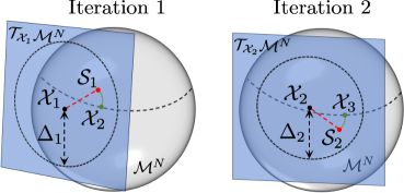
Figure 2: An illustration of two iterations of the RTR algorithm. At each iteration, the algorithm computes a tangent step $\mathcal{S}_{k}\in\mathcal{T}_{\mathcal{X}_{k}}\mathcal{M}$, shown in red, within a trust region of radius $\Delta_{k}$, which is indicated by the dotted circle shown in each tangent space. If the step is accepted (as defined in (17)), then the next iterate is computed as $\mathcal{X}_{k+1}=\mathrm{Exp}_{\mathcal{X}_{k}}(\mathcal{S}_{k})$, which maps the step from the tangent space back to the manifold itself, as shown in green.

An illustration of the proposed RTR algorithm is shown in Figure 2. At each iteration $k$, instead of approximating the objective $\mathcal{F}$, RTR computes an approximation of $\mathcal{F}$ in the tangent space at $\mathcal{X}_{k}$, called a pullback. The pullback is defined as $\hat{\mathcal{F}}_{k}\triangleq\mathcal{F}\circ\textnormal{Exp}_{\mathcal{X}_{k}}$. The approximation takes the form of a second-order model $\hat{m}_{k}:\mathcal{T}_{\mathcal{X}_{k}}\rightarrow\mathbb{R}$, which is given by

$$\hat{m}_{k}(\mathcal{S})\triangleq\mathcal{F}\left(\mathcal{X}_{k}\right)+\mathcal{S}^{\top}\textnormal{grad}\,\mathcal{F}\left(\mathcal{X}_{k}\right)+\frac{1}{2}\mathcal{S}^{\top}\mathcal{H}_{k}\mathcal{S},$$ (13)

where $\mathcal{S}\in\mathcal{T}_{\mathcal{X}_{k}}\mathcal{M}^{N}$ is a tangent vector centered at $\mathcal{X}_{k}$, $\textnormal{grad}\,\mathcal{F}:\mathcal{M}^{N}\rightarrow\mathcal{T}_{\mathcal{X}_{k}}\mathcal{M}^{N}$ is the Riemannian gradient, and $\mathcal{H}_{k}:\mathcal{T}_{\mathcal{X}_{k}}\mathcal{M}^{N}\rightarrow\mathcal{T}_{\mathcal{X}_{k}}\mathcal{M}^{N}$ is a symmetric approximation of the Riemannian Hessian at $\mathcal{X}_{k}$. We include explicit forms for $\textnormal{grad}\,\mathcal{F}$ in Appendix E and our choice of $\mathcal{H}_{k}$ in Appendix F-B

Our procedure corresponds to the RTR update given in [26, Chapter 7]. The algorithm is initialized with $\mathcal{X}_{0}\in\mathcal{M}^{N}$ and trust-region radius $\Delta_{0}\in\left(0,\bar{\Delta}\right]$, where $\bar{\Delta}>0$ is the user-specified maximum radius. At iteration $k$, the tentative step $\mathcal{S}_{k}$ is computed by solving the inner sub-problem

$$\mathcal{S}_{k}=\operatorname*{arg\,min}_{\mathcal{S}\in\mathcal{T}_{\mathcal{X}_{k}}\mathcal{M}^{N}}\hat{m}_{k}\left(\mathcal{S}\right)\text{\leavevmode\nobreak\ subject\leavevmode\nobreak\ to\leavevmode\nobreak\ }{\left\|\mathcal{S}\right\|}_{2}\leq\Delta_{k},$$ (14)

where $\hat{m}_{k}$ is from (13). To solve (14), we employ the Steihaug-Toint truncated conjugate gradients (tCG) algorithm [29, 30], which offers unique benefits for trust-region sub-problems, including monotonic cost decrease and early termination (thereby approximating (14)) in the cases of negative curvature or trust region violation. To measure the agreement between the model and objective functions, we use

$$\rho_{k}=\frac{\hat{\mathcal{F}}_{k}\left(\mathbf{0}\right)-\hat{\mathcal{F}}_{k}\left(\mathcal{S}_{k}\right)}{\hat{m}_{k}\left(\mathbf{0}\right)-\hat{m}_{k}\left(\mathcal{S}_{k}\right)},$$ (15)

where $\mathbf{0}\in\mathbb{R}^{4N}$ is the zero vector. Based on the level of agreement, the trust-region radius $\Delta_{k}$ is then updated via

$$\Delta_{k+1}=\begin{cases}\frac{1}{4}\Delta_{k}&\text{if\leavevmode\nobreak\ }\rho_{k}<\frac{1}{4}\\ \min\left\{2\Delta_{k},\bar{\Delta}\right\}&\text{if\leavevmode\nobreak\ }\rho_{k}>\frac{3}{4}\text{\leavevmode\nobreak\ and\leavevmode\nobreak\ }{\left\|\mathcal{S}_{k}\right\|}_{2}=\Delta_{k}\\ \Delta_{k}&\text{otherwise.}\end{cases}$$ (16)

The tentative step $\mathcal{S}_{k}$ is accepted to compute $\mathcal{X}_{k+1}$ only if the model agreement ratio $\rho_{k}$ from (15) is greater than a user-defined model agreement threshold $\rho^{\prime}\in\left(0,\nicefrac{{1}}{{4}}\right)$, i.e.,

$$\mathcal{X}_{k+1}=\begin{cases}\textnormal{Exp}_{\mathcal{X}_{k}}\!\left(\mathcal{S}_{k}\right)&\text{if\leavevmode\nobreak\ }\rho_{k}>\rho^{\prime}\\ \mathcal{X}_{k}&\text{otherwise.}\end{cases}$$ (17)

As summarized in Algorithm 1, the steps from (14)-(17) are repeated until the gradient norm crosses below a user-defined threshold $\varepsilon_{g}$, i.e., ${\left\|\operatorname{grad}\mathcal{F}\left(\mathcal{X}_{k}\right)\right\|}_{2}\leq\varepsilon_{g}$.

Input: Edge measurement set $\mathcal{Z}\in\mathcal{M}^{M}$,

Maximum trust-region radius $\bar{\Delta}>0$,

Model agreement threshold $\rho^{\prime}\in\left(0,\nicefrac{{1}}{{4}}\right]$,

Gradient termination threshold $\varepsilon_{g}>0$.

Initialize: $k\leftarrow 0$, $\mathcal{X}_{0}\in\mathcal{M}^{N}$, $\Delta_{0}\in\left(0,\bar{\Delta}\right]$

while ${\left\|\textnormal{grad}\,\mathcal{F}\left(\mathcal{X}_{k}\right)\right\|}_{2}>\varepsilon_{g}$ do

       Compute $\mathcal{S}_{k}$ from (14) using tCG.

       Compute $\rho_{k}$ using (15).

       Compute $\Delta_{k+1}$ using (16).

       Compute $\mathcal{X}_{k+1}$ using (17).

       $k\leftarrow k+1$

end while

return $\mathcal{X}_{k}$

Algorithm 1 RTR for PUDQ PGO

V Convergence Analysis

In this section, we prove that Algorithm 1 is globally convergent. Specifically, given any initialization, it reaches a first-order critical point to within a user-specified tolerance in finite time. The authors of [28] proposed global rates of convergence for the RTR algorithm given a set of assumptions about the problem, so we treat these assumptions as sufficient conditions for convergence. For our proof, we will establish:

1. Lower-boundedness of $\mathcal{F}$ on $\mathcal{M}^{N}$.

2. Sufficient decrease in the model cost at each iteration.

3. A Lipschitz-type condition for gradients of pullbacks.

4. Radial linearity and boundedness of $\mathcal{H}_{k}$.

We will make each of these statements mathematically precise in the following analysis. Towards proving Condition 1, we first derive a lemma on continuity of $\mathcal{F}$.

Lemma 1.

The objective $\mathcal{F}$ is continuous on $\mathcal{M}^{N}$.

Proof: By inspection of (3) and (9)-(11), and continuity of “$\boxplus$” from (1) as a linear map, it suffices to show that $\textnormal{Log}_{\mathbbm{1}}\!$ is continuous on $\mathcal{M}$. While (3) and (4) contain discontinuities independently, we will show that their composition to form $\textnormal{Log}_{\mathbbm{1}}$ does not. Let $\phi_{1}\triangleq\arctan(r_{1},r_{0})$ (where ${\mathbf{r}}_{ij}=[r_{0},r_{1},r_{2},r_{3}]^{\top}$ denotes the element-wise map), and let $\phi_{2}\triangleq\mathrm{wrap}(\phi_{1})$. Then, we have discontinuities in $\phi_{1}$ at $(r_{0},r_{1})=(-1,0)$, in $\mathrm{wrap}(\phi_{1})$ at $\phi_{1}=\pm\nicefrac{{\pi}}{{2}}$, and in $(\gamma(\phi_{2}))^{-1}$ at $\phi_{2}=\pm\pi$. We now observe that $\mathrm{wrap}(-\pi)=\mathrm{wrap}(\pi)=0$, so $\lim_{(r_{0},r_{1})\rightarrow(-1,0)}\mathrm{wrap}(\phi_{1})=0$, thereby nullifying the discontinuities in $\phi_{1}$. Next, $(\mathrm{sinc}(\phi_{2}))^{-1}$ is even and continuous on the domain $[\nicefrac{{-\pi}}{{2}},\nicefrac{{\pi}}{{2}}]$, so $\lim_{\phi_{2}\rightarrow\nicefrac{{-\pi}}{{2}}}(\gamma(\phi_{2}))^{-1}=\lim_{\phi_{2}\rightarrow\nicefrac{{\pi}}{{2}}}(\gamma(\phi_{2}))^{-1}=\nicefrac{{\pi}}{{2}}$, nullifying the discontinuities in $\phi_{2}$. Finally, because $\lim_{\phi_{2}\rightarrow 0}(\gamma(\phi_{2}))^{-1}=1$ and, by (4), $\phi_{2}\in(\nicefrac{{-\pi}}{{2}},\nicefrac{{-\pi}}{{2}}]$, we conclude that $\textnormal{Log}_{\mathbbm{1}}\!$ is continuous on $\mathcal{M}$, which implies that $\mathcal{F}$ is continuous on $\mathcal{M}^{N}$. $\blacksquare$

We now show compactness of sublevel sets of $\mathcal{F}$.

Theorem 1.

The $\mu$-sublevel sets of $\mathcal{F}$, given by $\left\{\mathcal{X}\mid\mathcal{F}\left(\mathcal{X}\right)\leq\mu\right\}$, are compact.

Proof: From (7), for every $\mathcal{X}\in\mathcal{M}^{N}$, $\textnormal{Exp}_{\mathcal{X}}$ is defined on the entire tangent space $\mathcal{T}_{\mathcal{X}}\mathcal{M}^{N}$, which implies that $\mathcal{M}^{N}$ is geodesically complete. Therefore, the Hopf-Rinow Theorem [31] implies that closed and bounded subsets of $\mathcal{M}^{N}$ are compact, and we will prove compactness of sublevel sets by proving that they are closed and bounded.

From (9)-(10), $\mathcal{F}\left(\mathcal{X}\right)\geq 0$ for all $\mathcal{X}\in\mathcal{M}^{N}$, which implies that the $\mu$-sublevel sets of $\mathcal{F}$ are the preimages of the closed subsets $[0,\mu]$, i.e., $\mu$-sublevel sets are of the form $\mathcal{F}^{-1}\big{(}[0,\mu]\big{)}$. These sets are closed because $\mathcal{F}$ is continuous by Lemma 1.

Turning to boundedness of sublevel sets, (2) implies that $\mathcal{M}$ is unbounded, and therefore $\mathcal{M}^{N}$ is unbounded. Then, by [32, Theorem 1], the $\mu$-sublevel sets are bounded if and only if $\mathcal{F}$ is coercive, i.e., for all $\mathcal{Y}\in\mathcal{M}^{N}$, every sequence $\{\mathcal{X}_{l}\}_{l\in\mathbb{N}}\subset\mathcal{M}^{N}$ such that $\lim_{l\rightarrow\infty}d_{\mathcal{M}^{N}}\left(\mathcal{X}_{l},\mathcal{Y}\right)=\infty$ also satisfies $\lim_{l\rightarrow\infty}F(\mathcal{X}_{l})=\infty$. Therefore, it suffices to show that $\mathcal{F}$ is coercive, which we do next.

First, let $\mathcal{X}_{l}=\operatorname{vec}\left((\mathbf{x}_{l,i})_{i\in\mathcal{V}}\right)$ and $\mathcal{Y}=\operatorname{vec}\left((\mathbf{y}_{i})_{i\in\mathcal{V}}\right)$, and observe from the definition of $d_{\mathcal{M}^{N}}\left(\mathcal{X}_{l},\mathcal{Y}\right)$ that

$$\lim_{d_{\mathcal{M}^{N}}\left(\mathcal{X}_{l},\mathcal{Y}\right)\rightarrow\infty}\max_{i\in\mathcal{V}}\|\textnormal{Log}_{\mathbbm{1}}\!(\mathbf{x}_{l,i}^{-1}\boxplus\mathbf{y}_{i})\|_{2}^{2}=\infty.$$ (18)

We now rewrite $\|\textnormal{Log}_{\mathbbm{1}}\!(\mathbf{x}_{l,i}^{-1}\boxplus\mathbf{y}_{i})\|_{2}^{2}$ as

$$\|\textnormal{Log}_{\mathbbm{1}}\!(\mathbf{x}_{l,i}^{-1}\boxplus\mathbf{y}_{i})\|_{2}^{2}=\gamma(\mathbf{x}_{l,i}^{-1}\boxplus\mathbf{y}_{i})^{-2}\mathbf{x}_{l,i}^{\top}M_{LR}^{-}(\mathbf{y}_{i})\mathbf{x}_{l,i},$$ (19)

where $M_{LR}^{-}(\mathbf{y}_{i})\triangleq Q_{LR}^{-}\left(\mathbf{y}_{i}\right)^{\top}\mathrm{diag}\left(\left\{0,I_{3}\right\}\right)Q_{LR}^{-}\left(\mathbf{y}_{i}\right)$, with $Q_{LR}^{-}\left(\mathbf{y}_{i}\right)$ given in Appendix A. Since $\gamma\left(\mathbf{x}\right)\in\left[\nicefrac{{-\pi}}{{2}},\nicefrac{{\pi}}{{2}}\right]$ for all $\mathbf{x}\in\mathcal{M}$, we have

$$\|\textnormal{Log}_{\mathbbm{1}}\!(\mathbf{x}_{l,i}^{-1}\boxplus\mathbf{y}_{i})\|_{2}^{2}\leq(\nicefrac{{\pi^{2}}}{{4}})\lambda_{max}(M_{LR}^{-}(\mathbf{y}_{i}))\mathbf{x}_{l,i}^{\top}\mathbf{x}_{l,i},$$ (20)

where $\lambda_{max}\left(\cdot\right)$ denotes the maximum eigenvalue of a matrix. Since $\mathbf{y}_{i}$ is constant and $\lambda_{max}(M_{LR}^{-}(\mathbf{y}_{i}))\geq 0$, (20) implies that $\lim_{\|\textnormal{Log}_{\mathbbm{1}}\!(\mathbf{x}_{l,i}^{-1}\boxplus\mathbf{y}_{i})\|_{2}^{2}\rightarrow\infty}(\mathbf{x}_{l,i}^{\top}\mathbf{x}_{l,i})=\infty$. The first element of $\mathbf{x}_{l,i}\in\mathcal{M}$ is bounded by $1$, so $\mathbf{x}_{l,i}^{\top}\mathbf{x}_{l,i}-1\leq\|\textnormal{Log}_{\mathbbm{1}}\!\left(\mathbf{x}_{l,i}\right)\|_{2}^{2}$. Therefore, $\lim_{(\mathbf{x}_{l,i}^{\top}\mathbf{x}_{l,i})\rightarrow\infty}\|\textnormal{Log}_{\mathbbm{1}}\!(\mathbf{x}_{l,i})\|_{2}^{2}=\infty$. Now, we note that for any $\mathbf{x},\mathbf{y}\in\mathcal{M}$, we can write

$$\left\|\textnormal{Log}_{\mathbbm{1}}\!\left(\mathbf{x}\boxplus\mathbf{y}\right)\right\|_{2}^{2} =\gamma\left(\mathbf{x}\boxplus\mathbf{y}\right)^{-1}\mathbf{y}^{\top}M_{L}\left(\mathbf{x}\right)\mathbf{y}$$ (21)

$$=\gamma\left(\mathbf{x}\boxplus\mathbf{y}\right)^{-1}\mathbf{x}^{\top}M_{R}\left(\mathbf{y}\right)\mathbf{x},$$ (22)

where $M_{L}\left(\mathbf{x}\right)\triangleq Q_{L}\left(\mathbf{x}\right)^{\top}\mathrm{diag}\left(\left\{0,I_{3}\right\}\right)Q_{L}\left(\mathbf{x}\right)$ and $M_{R}\left(\mathbf{y}\right)\triangleq Q_{R}\left(\mathbf{y}\right)^{\top}\mathrm{diag}\left(\left\{0,I_{3}\right\}\right)Q_{R}\left(\mathbf{y}\right)$. Because $M_{L}(\cdot),M_{R}(\cdot)\succeq 0$, it holds that, for any $\mathbf{x},\mathbf{y}\in\mathcal{M}$,

$$\lim_{\left\|\textnormal{Log}_{\mathbbm{1}}\!\left(\mathbf{x}\boxplus\mathbf{y}\right)\right\|_{2}^{2}\rightarrow\infty}\max\left\{\left\|\textnormal{Log}_{\mathbbm{1}}\!\left(\mathbf{x}\right)\right\|_{2}^{2},\left\|\textnormal{Log}_{\mathbbm{1}}\!\left(\mathbf{y}\right)\right\|_{2}^{2}\right\}=\infty.$$ (23)

We now observe that for any two vertices $\mathbf{x}_{i},\mathbf{x}_{j}\in\mathcal{M}$, with $i,j\in\mathcal{V}$ and $i>j$, it follows from connectedness of odometry edges in $\mathcal{E}$ that $\mathbf{x}_{i}=\mathbf{x}_{j}\boxplus\mathbf{c}_{i,j}$, where

$$\mathbf{c}_{i,j}\triangleq\tilde{\mathbf{z}}_{j(j+1)}\boxplus\mathbf{r}_{(j+1)(j+2)}\boxplus\cdots\boxplus\mathbf{\tilde{z}}_{\left(i-1\right)i}\boxplus\mathbf{r}_{\left(i-1\right)i}.$$ (24)

Equivalently, we have $\mathbf{x}_{j}=\mathbf{x}_{i}\boxplus\mathbf{c}_{i,j}^{-1}$. Per Section III, we have anchored $\mathbf{x}_{a}\triangleq\mathbbm{1}$ for some $a\in\mathcal{V}$, and since $\textnormal{Log}_{\mathbbm{1}}\!(\mathbf{x}^{-1})=-\textnormal{Log}_{\mathbbm{1}}\!(\mathbf{x})$, it holds that $\|\textnormal{Log}_{\mathbbm{1}}\!(\mathbf{x}_{l,m})\|_{2}^{2}=\|\textnormal{Log}_{\mathbbm{1}}\!(\mathbf{c}_{a,m})\|_{2}^{2}$ for any $m\in\mathcal{V}$. Furthermore, because the $\tilde{\mathbf{z}}_{ij}$ terms in (24) are constant, applying (23) inductively yields, for any $m\in\mathcal{V}$,

$$\lim_{\left\|\textnormal{Log}_{\mathbbm{1}}\!\left(\mathbf{x}_{l,m}\right)\right\|_{2}^{2}\rightarrow\infty}\max_{\left(i,j\right)\in\mathcal{E}}\left\|\textnormal{Log}_{\mathbbm{1}}\!\left(\mathbf{r}_{i,j}\right)\right\|_{2}^{2}=\infty.$$ (25)

From (10), we have $\lambda_{min}\left(\Omega_{ij}\right)\left\|\textnormal{Log}_{\mathbbm{1}}\!\left(\mathbf{r}_{i,j}\right)\right\|_{2}^{2}\leq f_{ij}\left(\mathcal{X}_{l}\right)$, where $\lambda_{min}(\cdot)$ is the minimum eigenvalue of a matrix, and $\lambda_{min}(\Omega_{ij})>0$ because it is an information matrix. Then $\lim_{\|\textnormal{Log}_{\mathbbm{1}}\!(\mathbf{r}_{ij})\|_{2}^{2}\rightarrow\infty}f_{ij}(\mathcal{X}_{l})=\infty$, and from (9) we have $\lim_{f_{ij}(\mathcal{X}_{l})\rightarrow\infty}\mathcal{F}(\mathcal{X}_{l})=\infty$. Then $\mathcal{F}$ is coercive and the proof is complete. $\blacksquare$

Theorem 1 implies the following corollary.

Corollary 1.

Given any initialization $\mathcal{X}_{0}\in\mathcal{M}^{N}$, the $\mathcal{F}\left(\mathcal{X}_{0}\right)$-sublevel set $\left\{\mathcal{X}\mid\mathcal{F}\left(\mathcal{X}\right)\leq\mathcal{F}\left(\mathcal{X}_{0}\right)\right\}$ is compact.

In the following lemma, we apply Lemma 1 and Theorem 1 to show that the objective $\mathcal{F}$ satisfies Condition 1.

Lemma 2.

There exists $\mathcal{F}^{\star}\geq 0$ such that $\mathcal{F}\left(\mathcal{X}\right)\geq\mathcal{F}^{\star}$ for all $\mathcal{X}\in\mathcal{M}^{N}$.

Proof: Lemma 1, Theorem 1, and the Weierstrass Theorem [33, Prop. A.8] imply the existence of a global minimizer $\mathcal{X}^{\star}\in\mathcal{M}^{N}$, which is the solution to Problem 1. Setting $\mathcal{F}^{\star}\triangleq\mathcal{F}\left(\mathcal{X}^{\star}\right)$ completes the proof.  $\blacksquare$

We now show that Algorithm 1 easily satisfies Condition 2.

Lemma 3.

For all $\mathcal{X}_{k}$ computed by Algorithm 1 such that ${\left\|\textnormal{grad}\,\mathcal{F}\left(\mathcal{X}_{k}\right)\right\|}_{2}>\varepsilon_{g}$, it holds that the step $\mathcal{S}_{k}$ satisfies

$$\hat{m}_{k}\left(\mathbf{0}\right)-\hat{m}_{k}\left(\mathcal{S}_{k}\right)\geq\frac{1}{2}\min\{\Delta_{k},2\varepsilon_{g}\}\varepsilon_{g}.$$ (26)

Proof: By design, iterates of the tCG algorithm produce a strict, monotonic decrease of the model cost $\hat{m}_{k}$ [28]. For all $k$, the first tCG iterate is the Cauchy step, which satisfies (26) by definition and thus completes the proof. $\blacksquare$

The forthcoming analysis in Lemma 4, Theorem 2, and Lemma 5 addresses Condition 3, namely, Lipschitz continuity of the Riemannian gradient, $\textnormal{grad}\,\mathcal{F}$. First, we use Theorem 2 to prove its Lipschitz continuity on compact subsets of $\mathcal{M}^{N}$.

Theorem 2.

The Riemannian gradient, $\textnormal{grad}\,\mathcal{F}$, is $L_{g}$-Lipschitz continuous on any compact subset $\mathcal{K}\subset\mathcal{M}^{N}$. That is, there exists $L_{g}>0$ such that for all $\mathcal{X},\mathcal{Y}\in\mathcal{K}$ we have

$${\left\|\mathcal{P}_{\mathcal{X}\rightarrow\mathcal{Y}}\textnormal{grad}\,\mathcal{F}\left(\mathcal{X}\right)-\textnormal{grad}\,\mathcal{F}\left(\mathcal{Y}\right)\right\|}_{2}\leq L_{g}d_{\mathcal{M}^{N}}\left(\mathcal{X},\mathcal{Y}\right),$$ (27)

where $\mathcal{P}_{\mathcal{X}\rightarrow\mathcal{Y}}:\mathcal{T}_{\mathcal{X}}\mathcal{M}^{N}\rightarrow\mathcal{T}_{\mathcal{Y}}\mathcal{M}^{N}$ is the parallel transport operator defined in Appendix B-E.

Proof: A necessary and sufficient condition for (27) is that, for all $\mathcal{X}\in\mathcal{K}$, the Riemannian Hessian, $\textnormal{Hess}\,\mathcal{F}$, has operator norm bounded by $L_{g}$, i.e.,

$$\sup_{\mathcal{V}\in\mathcal{T}_{\mathcal{X}}\mathcal{M},\|\mathcal{V}\|_{2}=1}\left\|\text{Hess}\leavevmode\nobreak\ \mathcal{F}(\mathcal{X})[\mathcal{V}]\right\|_{2}\leq L_{g}.$$ (28)

In Appendix F, we derive $\textnormal{Hess}\,\mathcal{F}$, and in Appendix G, we derive a constant $L_{g}$ for which (28) holds on any compact subset $\mathcal{K}\subset\mathcal{M}^{N}$, completing the proof. $\blacksquare$

To apply Theorem 2 to Algorithm 1, we must first show that the computed iterates remain within the $\mathcal{F}\left(\mathcal{X}_{0}\right)$-sublevel set for all $k$, which is accomplished by Lemma 4.

Lemma 4.

The objective $\mathcal{F}$ is monotonically decreasing with respect to the iterates of Algorithm 1. In particular, it holds that $\mathcal{F}\left(\mathcal{X}_{k}\right)\leq\mathcal{F}\left(\mathcal{X}_{0}\right)$ for all $k$.

Proof: By (26), we have $\hat{m}_{k}\left(\mathbf{0}\right)-\hat{m}_{k}\left(\mathcal{S}_{k}\right)>0$ for all $k$. If any $\mathcal{S}_{k}$ would yield an increase in $\mathcal{F}$, then $\mathcal{F}\left(\mathcal{X}_{k}\right)-\mathcal{F}(\mathrm{Exp}_{\mathcal{X}_{k}}(\mathcal{S}_{k}))<0$, and (15) implies $\rho_{k}<0$. By (17), such an $\mathcal{S}_{k}$ is rejected and, therefore the condition $\mathcal{F}(\mathcal{X}_{k+1})=\mathcal{F}\left(\mathcal{X}_{k}\right)$ is enforced in such cases. Thus, since it cannot occur that $\mathcal{F}(\mathcal{X}_{k+1})>\mathcal{F}(\mathcal{X}_{k})$, we see that $\mathcal{F}(\mathcal{X}_{k+1})\leq\mathcal{F}\left(\mathcal{X}_{k}\right)$ for all $k$. By induction, $\mathcal{F}\left(\mathcal{X}_{k}\right)\leq\mathcal{F}\left(\mathcal{X}_{0}\right)$ for all $k$, completing the proof. $\blacksquare$

Now, Lemma 5 extends Theorem 2 to any $\mathcal{X}_{k}$ computed by Algorithm 1, which shows that Condition 3 is satisfied.

Lemma 5.

For all $\mathcal{X}_{k}$ computed by Algorithm 1, there exists $L_{g}\geq 0$ such that

$$\left|\mathcal{F}\left(\textnormal{Exp}_{\mathcal{X}_{k}}\!\left(\mathcal{S}\right)\right)-\left(\mathcal{F}\left(\mathcal{X}_{k}\right)+\mathcal{S}^{\top}\textnormal{grad}\,\mathcal{F}\left(\mathcal{X}_{k}\right)\right)\right|\leq\frac{L_{g}}{2}{\left\|\mathcal{S}\right\|}_{2}^{2}$$ (29)

for all $\mathcal{S}\in\mathcal{T}_{\mathcal{X}_{k}}\mathcal{M}^{N}$ such that ${\left\|\mathcal{S}\right\|}_{2}\leq\bar{\Delta}$ and for all $k$.

Proof: Let $M_{\mathcal{X}_{0}}\triangleq\left\{\mathcal{X}\mid\mathcal{F}\left(\mathcal{X}\right)\leq\mathcal{F}\left(\mathcal{X}_{0}\right)\right\}$ and set

$$\mathcal{K}\triangleq M_{\mathcal{X}_{0}}\cup\{\textnormal{Exp}_{\mathcal{X}}\!\left(\mathcal{S}\right)\mid\mathcal{X}\in M_{\mathcal{X}_{0}},{\left\|\mathcal{S}\right\|}_{2}\leq\bar{\Delta}\}.$$ (30)

Then Theorem 1 implies that $M_{\mathcal{X}_{0}}$ is compact, and therefore so is $\mathcal{K}$. Lemma 4 implies $\mathcal{X}_{k}\in M_{\mathcal{X}_{0}}\subset\mathcal{K}$ for all $k$. By Theorem 2, there exists $L_{g}>0$ to which (27) applies for all $\mathcal{X}_{k}\in\mathcal{K}$. From [34, Lemma 2.1], we find that (27) implies (29), completing the proof. $\blacksquare$

Lemmas 6 and 7 address Condition 4, which pertains to properties of $\mathcal{H}_{k}$, the Riemannian Hessian approximation used in (14) and spelled out in Appendix F-B.

Lemma 6.

The operator $\mathcal{H}_{k}$ in 205 is radially linear, i.e., for all $\mathcal{S}\in\mathcal{T}_{\mathcal{X}_{k}}\mathcal{M}^{N}$ and all $\alpha\geq 0$, we have $\mathcal{H}_{k}[\alpha\mathcal{S}]=\alpha\mathcal{H}_{k}[\mathcal{S}]$.

Proof: Equation (205) is linear by inspection. $\blacksquare$

Lemma 7.

The operator $\mathcal{H}_{k}$ in (205) is bounded for all $\mathcal{X}_{k}$ computed by Algorithm 1, i.e., there exists $\beta<\infty$ such that

$$\max_{\mathcal{S}}\Big{\{}\|\mathcal{H}_{k}\mathcal{S}\|_{2}\mid\mathcal{S}\in\mathcal{T}_{\mathcal{X}_{k}}\mathcal{M}^{N},{\left\|\mathcal{S}\right\|}_{2}=1\Big{\}}\leq\beta.$$ (31)

Proof: First, $\left\|\mathcal{S}\right\|_{2}=1$ implies $\left\|\mathcal{H}_{k}\mathcal{S}\right\|_{2}\leq\left\|\mathcal{H}_{k}\right\|_{2}$. Substituting (205), applying the triangle inequality, and using the fact that $\lambda_{max}\left(\mathcal{P}_{\mathcal{X}}\right)=1$ yields

$$\left\|\mathcal{H}_{k}\right\|_{2}\leq\sum_{\left(i,j\right)\in\mathcal{E}}\left\|\mathcal{P}_{\mathcal{X}}\mathcal{R}_{ij}\mathcal{P}_{\mathcal{X}}\right\|_{2}\leq\sum_{\left(i,j\right)\in\mathcal{E}}\left\|\mathcal{R}_{ij}\right\|_{2}.$$ (32)

Since, by definition of $\|\cdot\|_{2}$ and $\|\cdot\|_{F}$ we have $\|\mathcal{R}_{ij}\|_{2}\leq\|\mathcal{R}_{ij}\|_{F}$, we reach

$$\left\|\mathcal{R}_{ij}\right\|_{2}\leq 4\left\|\mathcal{A}_{ij}\right\|_{F}\left\|\mathcal{B}_{ij}\right\|_{F}\left\|\Omega_{ij}\right\|_{F}.$$ (33)

Now, we set $\mathcal{K}$ as in (30) and apply the bounds derived in Appendix J for $\left\|\mathcal{A}_{ij}\right\|_{F}$ and $\left\|\mathcal{B}_{ij}\right\|_{F}$ on compact subsets of $\mathcal{M}^{N}$. Since every term on the right-hand side of (33) is bounded, we see that the right-hand side of (32) is bounded, completes the proof. $\blacksquare$

Our convergence analysis culminates in Theorem 3.

Theorem 3.

Let $\varepsilon_{g}\leq\nicefrac{{\Delta_{0}}}{{\lambda_{g}}}$ be given, where $\Delta_{0}$ is from Section IV, $\lambda_{g}\triangleq\nicefrac{{1}}{{4}}\min\left\{\nicefrac{{1}}{{\beta}},\nicefrac{{1}}{{2(L_{g}+\beta)}}\right\}$, $L_{g}$ is from (29), and $\beta$ is from (31). Then, for any initialization $\mathcal{X}_{0}\in\mathcal{M}^{N}$, Algorithm 1 produces an iterate $\mathcal{X}_{k}$ that satisfies $\left\|\textnormal{grad}\,\mathcal{F}(\mathcal{X}_{k})\right\|_{2}\leq\varepsilon_{g}$ in no more than $K$ iterations, where

$$K\leq\frac{\mathcal{F}\left(\mathcal{X}_{0}\right)-\mathcal{F}\left(\mathcal{X}^{\star}\right)}{\rho^{\prime}\lambda_{g}}\frac{3}{\varepsilon_{g}^{2}}+\frac{1}{2}\log_{2}\left(\frac{\Delta_{0}}{\lambda_{g}\varepsilon_{g}}\right),$$ (34)

where $\rho^{\prime}$ is from (17) and $\mathcal{X}^{\star}$ is from Lemma 2.

Proof: Lemmas 2, 3, and 5-7 show the satisfaction of Conditions 1-4 in [28, Theorem 12], which immediately implies that (34) holds for Algorithm 1. $\blacksquare$

Theorem 3 gives provable convergence of Algorithm 1 to approximate first-order critical points of $\mathcal{F}$ under any initialization $\mathcal{X}_{0}$, and we note that the tolerance $\varepsilon_{g}$ can be made to take arbitrary values by adjusting $\Delta_{0}$.

VI Experimental Results

In this section, we validate the accuracy of Algorithm 1 relative to the Riemannian PGO solvers SE-Sync [13] and Cartan-Sync [14]. Both yield a global minimizer identical to that computed by the class of Riemannian algorithms that use semidefinite relaxations (e.g., [15, 35]), so we omit additional comparisons to those algorithms.

The comparisons we present necessitated the use of exact ground truth, which prevented the use of experimentally-generated datasets. Therefore, we evaluate performance using three synthetic PGO datasets with diverse vertex and edge counts. The first of these is Grid1000, which we synthesized with $N=1000$ vertices and $M=1250$ edges. The remaining datasets are publicly available, and serve as common benchmarks for PGO evaluations, namely, (i) M3500 [36], with $N=3500$, $M=5598$, and (ii) City10000 [12], with $N=10000$, $M=20687$. To generate PGO trial datasets, we apply measurement noise to the ground truth dataset for each graph. Each of these datasets, including ground truth, is available at https://github.com/corelabuf/planar_pgo_datasets.

VI-A PGO dataset generation

To generate a PGO dataset, the true edge measurements from each dataset are corrupted using the Lie-theoretic noise model from (8), and the edge measurement noise covariance, $\Sigma_{ij}$, is computed as $\Sigma_{ij}\sim W_{3}\left(\sigma_{w}\Sigma_{w},10\right)$, where $W_{d}\left(V,n\right)$ is the Wishart distribution with dimension $d$, scale matrix $V$, and $n$ degrees of freedom. Here, $\sigma_{w}$ is a variance tuning parameter, and $\Sigma_{w}$ is given by $\Sigma_{w}\triangleq J_{3}+\mathrm{diag}\left(\left[u_{1},u_{2},u_{3}\right]\right)$, where $J_{3}\in\mathbb{R}^{3\times 3}$ is a matrix of ones and $u_{i}\sim\mathcal{U}_{(0,1]}$ are randomly sampled from a uniform distribution on the interval $(0,1]$. This generates random, positive-definite covariance matrices with $\mathbb{E}[\Sigma_{ij}]=10\sigma_{w}\Sigma_{w}$, and ensures diagonal dominance of $\Sigma_{w}$ with anisotropic variances. Our approach simulates relative pose covariances computed by a Lie-theoretic estimator, leading to realistic pose graph depictions. Figure 3 depicts an M3500 variant generated with $\sigma_{w}=5.62\cdot 10^{-5}$ beside the estimate computed by Algorithm 1.

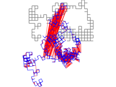
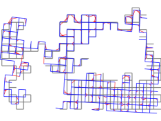
Figure 3: (Left) The M3500 pose graph dataset, corrupted with Lie-theoretic noise. (Right) The estimated graph computed by Algorithm 1. Odometry edges are blue, loop closures are red, and ground truth is shown in gray.

VI-B Evaluation methodology

Solutions computed by each algorithm were evaluated using the root-mean square relative pose error (RPE) metric. RPE measures total edge deformation with respect to the ground truth, and has been shown to be an objective performance metric for SLAM algorithms [38, 39]. We use $\left\{\mathbf{x}_{i}^{\diamond}\right\}_{i=1}^{N}$ to denote the ground truth pose set, and $\left\{\hat{\mathbf{x}}_{i}\right\}_{i=1}^{N}$ to be a solution computed by a given algorithm. The Lie-theoretic RPE, denoted RPE-L, is defined as

$$\text{RPE-L}=\sqrt{\frac{1}{M}\sum_{\left(i,j\right)\in\mathcal{E}}{\left\|\textnormal{Log}_{\mathbbm{1}}\!\left(\hat{\mathbf{z}}_{ij}^{-1}\boxplus\mathbf{z}_{ij}^{\diamond}\right)\right\|}_{2}^{2}},$$ (35)

where $\hat{\mathbf{z}}_{ij}\triangleq\hat{\mathbf{x}}_{i}^{-1}\boxplus\hat{\mathbf{x}}_{j}$ and $\mathbf{z}_{ij}^{\diamond}\triangleq(\mathbf{x}_{i}^{\diamond})^{-1}\boxplus\mathbf{x}_{j}^{\diamond}$. Now, let $(\hat{\mathbf{t}}_{i},\hat{\theta}_{i})$ and $(\mathbf{t}_{i}^{\diamond},\theta_{i}^{\diamond})$ denote the translations and rotations corresponding to $\hat{\mathbf{x}}_{i}$ and $\mathbf{x}_{i}^{\diamond}$, respectively. The Euclidean RPE, denoted RPE-E, is defined as

$$\text{RPE-E}=\sqrt{\frac{1}{M}\sum_{\left(i,j\right)\in\mathcal{E}}\left(\left\|\hat{\mathbf{t}}_{ij}-\mathbf{t}_{ij}^{\diamond}\right\|^{2}+d(\hat{\theta}_{ij},\theta_{ij}^{\diamond})^{2}\right)},$$ (36)

where $\hat{\mathbf{t}}_{ij}\triangleq R^{\top}(\hat{\theta}_{i})\left(\hat{\mathbf{t}}_{j}-\hat{\mathbf{t}}_{i}\right)$, $\mathbf{t}_{ij}^{\diamond}\triangleq R^{\top}\left(\theta_{i}^{\diamond}\right)\left(\mathbf{t}_{j}^{\diamond}-\mathbf{t}_{i}^{\diamond}\right)$, $d\left(\theta_{1},\theta_{2}\right)$ is the minimal angle between $\theta_{1}$ and $\theta_{2}$, and

$$R\left(\theta\right)\triangleq\left[\begin{smallmatrix}\cos\left(\theta\right)&-\sin\left(\theta\right)\\ \sin\left(\theta\right)&\cos\left(\theta\right)\end{smallmatrix}\right].$$ (37)

We synthesized 5 noisy trial datasets per ground truth trajectory, for a total of 15 datasets for comparison. For each dataset, the variance scaling parameter, $\sigma_{w}$, was varied from $1.0\cdot 10^{-5}$ to $3.16\cdot 10^{-2}$. For reference, this equated to Euclidean covariances with mean standard deviations ranging from $7.26\cdot 10^{-3}$ to $2.29\cdot 10^{-1}$ meters for translations, and from $4.05\cdot 10^{-1}$ to $12.81$ degrees for rotations.

For evaluation, we anchor $\mathbf{x}_{1}\triangleq\mathbbm{1}$ for all three algorithms. The initial iterate $\mathcal{X}_{0}$ is computed using the chordal relaxation [40] technique; though this is not necessary for convergence of Algorithm 1, it is the default for both SE-Sync and Cartan-Sync, so we implement it to provide a fair comparison. Algorithm 1 was configured with parameters $\varepsilon_{g}=10^{-2}$, $\Delta_{0}=100$, $\bar{\Delta}=10^{6}$, $\rho^{\prime}=10^{-2}$, and the inner tCG algorithm was implemented with parameters $\kappa=0.05$, $\theta=0.25$, per the notation in [24, Section 6.5].

VI-C Evaluation results

Algorithm 1 converged to an approximate stationary point in all of the $15$ pose graphs. The RPEs computed for each run according to (35) and (36) are included in Table I. We also include the percent reduction in RPE for each run, which is plotted in Figure 4. SE-Sync and Cartan-Sync computed identical solutions for each dataset, and exhibited a notable estimation bias across the entire noise spectrum, owing to the assumption of isotropic noise and the resulting approximation error. As shown in Figure 4, Algorithm 1 demonstrated a consistent 11%-26% reduction in RPE over comparable state-of-the-art algorithms. We also note that the gap in RPE increases with the number of vertices and edges in each graph, highlighting the scalability of our proposed solution.

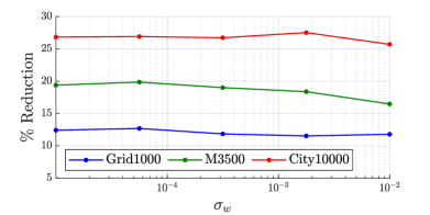
Figure 4: Percent reduction in Riemannian RPE for the solutions computed by Algorithm 1 relative to Cartan-Sync and SE-Sync. Reduction in Euclidean RPE was omitted due to it being indistinguishable from the Riemannian case. We see greater than $10$% decrease for the Grid1000 dataset over the entire noise regime, and greater than $18$% & $25$% for the M3500 and City10000 datasets, respectively. In all cases, the improvement in accuracy attained by Algorithm 1 grows with the number of vertices and edges present in a graph.

TABLE I: Results of the 2D PGO dataset evaluation. RPE and percent reduction in RPE attained by Algorithm 1 are shown on the right.

		SE-Sync [13]		Cartan-Sync [14]		Algorithm 1 [ours] (% Reduction)
Dataset	$\sigma_{w}$	RPE-L	RPE-E	RPE-L	RPE-E	RPE-L	RPE-E
Grid1000	$1.0\cdot 10^{-5}$	$6.2\cdot 10^{-3}$	$1.2\cdot 10^{-2}$	$6.2\cdot 10^{-3}$	$1.2\cdot 10^{-2}$	$5.4\cdot 10^{-3}$ ($\scalebox{0.75}[1.0]{$-$}12.4$%)	$1.1\cdot 10^{-2}$ ($\scalebox{0.75}[1.0]{$-$}12.4$%)
Grid1000	$5.6\cdot 10^{-5}$	$1.5\cdot 10^{-2}$	$2.9\cdot 10^{-2}$	$1.5\cdot 10^{-2}$	$2.9\cdot 10^{-2}$	$1.3\cdot 10^{-2}$ ($\scalebox{0.75}[1.0]{$-$}12.7$%)	$2.6\cdot 10^{-2}$ ($\scalebox{0.75}[1.0]{$-$}12.7$%)
Grid1000	$3.2\cdot 10^{-4}$	$3.5\cdot 10^{-2}$	$7.1\cdot 10^{-2}$	$3.5\cdot 10^{-2}$	$7.1\cdot 10^{-2}$	$3.1\cdot 10^{-2}$ ($\scalebox{0.75}[1.0]{$-$}11.8$%)	$6.2\cdot 10^{-2}$ ($\scalebox{0.75}[1.0]{$-$}11.8$%)
Grid1000	$1.8\cdot 10^{-3}$	$7.9\cdot 10^{-2}$	$1.6\cdot 10^{-1}$	$7.9\cdot 10^{-2}$	$1.6\cdot 10^{-1}$	$7.0\cdot 10^{-2}$ ($\scalebox{0.75}[1.0]{$-$}11.5$%)	$1.4\cdot 10^{-1}$ ($\scalebox{0.75}[1.0]{$-$}11.5$%)
Grid1000	$1.0\cdot 10^{-2}$	$1.9\cdot 10^{-1}$	$3.9\cdot 10^{-1}$	$1.9\cdot 10^{-1}$	$3.9\cdot 10^{-1}$	$1.7\cdot 10^{-1}$ ($\scalebox{0.75}[1.0]{$-$}11.8$%)	$3.4\cdot 10^{-1}$ ($\scalebox{0.75}[1.0]{$-$}11.7$%)
M3500	$1.0\cdot 10^{-5}$	$5.4\cdot 10^{-3}$	$1.1\cdot 10^{-2}$	$5.4\cdot 10^{-3}$	$1.1\cdot 10^{-2}$	$4.4\cdot 10^{-3}$ ($\scalebox{0.75}[1.0]{$-$}19.4$%)	$8.7\cdot 10^{-3}$ ($\scalebox{0.75}[1.0]{$-$}19.4$%)
M3500	$5.6\cdot 10^{-5}$	$1.3\cdot 10^{-2}$	$2.6\cdot 10^{-2}$	$1.3\cdot 10^{-2}$	$2.6\cdot 10^{-2}$	$1.0\cdot 10^{-2}$ ($\scalebox{0.75}[1.0]{$-$}19.8$%)	$2.1\cdot 10^{-2}$ ($\scalebox{0.75}[1.0]{$-$}19.8$%)
M3500	$3.2\cdot 10^{-4}$	$3.1\cdot 10^{-2}$	$6.2\cdot 10^{-2}$	$3.1\cdot 10^{-2}$	$6.2\cdot 10^{-2}$	$2.5\cdot 10^{-2}$ ($\scalebox{0.75}[1.0]{$-$}19.0$%)	$5.0\cdot 10^{-2}$ ($\scalebox{0.75}[1.0]{$-$}19.0$%)
M3500	$1.8\cdot 10^{-3}$	$7.4\cdot 10^{-2}$	$1.5\cdot 10^{-1}$	$7.4\cdot 10^{-2}$	$1.5\cdot 10^{-1}$	$6.0\cdot 10^{-2}$ ($\scalebox{0.75}[1.0]{$-$}18.4$%)	$1.2\cdot 10^{-1}$ ($\scalebox{0.75}[1.0]{$-$}18.4$%)
M3500	$1.0\cdot 10^{-2}$	$1.7\cdot 10^{-1}$	$3.4\cdot 10^{-1}$	$1.7\cdot 10^{-1}$	$3.4\cdot 10^{-1}$	$1.4\cdot 10^{-1}$ ($\scalebox{0.75}[1.0]{$-$}16.5$%)	$2.9\cdot 10^{-1}$ ($\scalebox{0.75}[1.0]{$-$}16.4$%)
City10k	$1.0\cdot 10^{-5}$	$4.9\cdot 10^{-3}$	$9.7\cdot 10^{-3}$	$4.9\cdot 10^{-3}$	$9.7\cdot 10^{-3}$	$3.6\cdot 10^{-3}$ ($\scalebox{0.75}[1.0]{$-$}26.8$%)	$7.1\cdot 10^{-3}$ ($\scalebox{0.75}[1.0]{$-$}26.8$%)
City10k	$5.6\cdot 10^{-5}$	$1.2\cdot 10^{-2}$	$2.3\cdot 10^{-2}$	$1.2\cdot 10^{-2}$	$2.3\cdot 10^{-2}$	$8.5\cdot 10^{-3}$ ($\scalebox{0.75}[1.0]{$-$}26.9$%)	$1.7\cdot 10^{-2}$ ($\scalebox{0.75}[1.0]{$-$}26.9$%)
City10k	$3.2\cdot 10^{-4}$	$2.8\cdot 10^{-2}$	$5.5\cdot 10^{-2}$	$2.8\cdot 10^{-2}$	$5.5\cdot 10^{-2}$	$2.0\cdot 10^{-2}$ ($\scalebox{0.75}[1.0]{$-$}26.7$%)	$4.0\cdot 10^{-2}$ ($\scalebox{0.75}[1.0]{$-$}26.7$%)
City10k	$1.8\cdot 10^{-3}$	$6.6\cdot 10^{-2}$	$1.3\cdot 10^{-1}$	$6.6\cdot 10^{-2}$	$1.3\cdot 10^{-1}$	$4.8\cdot 10^{-2}$ ($\scalebox{0.75}[1.0]{$-$}27.5$%)	$9.5\cdot 10^{-2}$ ($\scalebox{0.75}[1.0]{$-$}27.5$%)
City10k	$1.0\cdot 10^{-2}$	$1.6\cdot 10^{-1}$	$3.1\cdot 10^{-1}$	$1.6\cdot 10^{-1}$	$3.1\cdot 10^{-1}$	$1.2\cdot 10^{-1}$ ($\scalebox{0.75}[1.0]{$-$}25.7$%)	$2.3\cdot 10^{-1}$ ($\scalebox{0.75}[1.0]{$-$}25.7$%)

VII Conclusion

We presented a novel algorithm for planar PGO derived from a realistic, Lie-theoretic model for uncertainty on rigid motion groups. The proposed algorithm was proven to converge in finite-time to approximate first-order stationary points under any initialization, while requiring no additional assumptions about the problem. The proposed algorithm showed significantly improved accuracy relative to state-of-the-art algorithms, and these findings motivate further research into Riemannian PGO algorithms that use Lie-theoretic noise models. Future work will extend the algorithm to the 3D case and investigate distributed implementations.

Appendix A Algebraic Construction

Given an orthonormal basis $\{\mathbf{i},\mathbf{j},\mathbf{k}\}$, a rotation in the plane is characterized by a rotation angle $\theta\in(-\pi,\pi]$ about the $\mathbf{k}$ axis. In standard form, we can write the planar unit quaternion $\mathbf{q}\in\mathbb{S}^{1}$ corresponding to this rotation as

$$\mathbf{q}=\cos\left(\nicefrac{{\theta}}{{2}}\right)+\mathbf{k}\sin\left(\nicefrac{{\theta}}{{2}}\right)=r_{0}+\mathbf{k}r_{1},$$ (38)

or, in vector form, ${\mathbf{q}=\left[q_{0},q_{1}\right]}^{\top}$. Let “$\otimes$” denote the Hamilton product [23] under the convention $\mathbf{i}^{2}=\mathbf{j}^{2}=\mathbf{k}^{2}=\mathbf{i}\mathbf{j}\mathbf{k}=-1$. Then, performing the Hamiltonian multiplication of two planar quaternions, denoted $\mathbf{r},\mathbf{s}$, yields

$$\mathbf{r}\otimes\mathbf{s}=\left(r_{0}+\mathbf{k}r_{1}\right)\left(s_{0}+\mathbf{k}s_{1}\right)=r_{0}s_{0}-r_{1}s_{1}+\mathbf{k}\left(r_{1}s_{0}+r_{0}s_{1}\right)$$ (39)

In matrix-vector form, the operation can be written as

$$\mathbf{r}\otimes\mathbf{s} =\left[\begin{array}[]{cc}r_{0}&-r_{1}\\ r_{1}&r_{0}\end{array}\right]\left[\begin{array}[]{c}s_{0}\\ s_{1}\end{array}\right]=\left[\begin{array}[]{cc}s_{0}&-s_{1}\\ s_{1}&s_{0}\end{array}\right]\left[\begin{array}[]{c}r_{0}\\ r_{1}\end{array}\right].$$

A planar rigid motion is characterized by a translation, denoted $\mathbf{t}=t_{x}\mathbf{i}+t_{y}\mathbf{j}$, and a rotation about the $\mathbf{k}$ axis by an angle $\theta\in(-\pi,\pi]$. This can be written in $\mathbb{R}^{3}$ as the Euclidean vector $\mathbf{p}=[\mathbf{t}^{\top},\theta]^{\top}$. The planar unit dual quaternion (PUDQ) parameterization of this motion is given by $\mathbf{x}=\mathbf{x}_{r}+\epsilon\mathbf{x}_{d}$, where $\epsilon$ is a dual number satisfying $\epsilon^{2}=0,\epsilon\neq 0$. The real part of $\mathbf{x}$, denoted $\mathbf{x}_{r}\in\mathbb{S}^{1}$, is a planar unit quaternion of the form

$$\mathbf{x}_{r}=\cos\left(\nicefrac{{\theta}}{{2}}\right)+\sin\left(\nicefrac{{\theta}}{{2}}\right)\mathbf{k}=r_{0}+\mathbf{k}r_{1}.$$ (40)

The dual part of $\mathbf{x}$, denoted $\mathbf{x}_{d}\in\mathbb{R}^{2}$, is given by

$$\mathbf{x}_{d}=\frac{1}{2}\mathbf{t}\otimes\mathbf{x}_{r}=\frac{1}{2}\left(t_{x}\mathbf{i}+t_{y}\mathbf{j}\right)\left(r_{0}+\mathbf{k}r_{1}\right)=\frac{1}{2}\left(\left(t_{x}r_{0}+t_{y}r_{1}\right)\mathbf{i}+\left(t_{y}r_{0}-t_{x}r_{1}\right)\mathbf{j}\right).$$ (41)

In matrix-vector form, (41) can be rewritten as

$$\mathbf{x}_{d}=\frac{1}{2}\left[\begin{array}[]{cc}t_{x}&t_{y}\\ t_{y}&-t_{x}\end{array}\right]\left[\begin{array}[]{c}r_{0}\\ r_{1}\end{array}\right]=\frac{1}{2}\left[\begin{array}[]{cc}r_{0}&r_{1}\\ -r_{1}&r_{0}\end{array}\right]\left[\begin{array}[]{c}t_{x}\\ t_{y}\end{array}\right].$$ (42)

In vector form, a PUDQ can be expressed in terms of the bases $\{\mathbf{i},\mathbf{k},\epsilon\mathbf{i},\epsilon\mathbf{j}\}$ as

$$\mathbf{x}=x_{0}+\mathbf{k}x_{1}+\epsilon\left(\mathbf{i}x_{2}+\mathbf{j}x_{3}\right)={\left[x_{0},\leavevmode\nobreak\ x_{1},\leavevmode\nobreak\ x_{2},\leavevmode\nobreak\ x_{3}\right]}^{\top}.$$ (43)

Equivalently, we can write $\mathbf{x}=[\mathbf{x}_{r}^{\top},\mathbf{x}_{d}^{\top}]$. Given two PUDQs, $\mathbf{x}={\left[x_{0},\leavevmode\nobreak\ x_{1},\leavevmode\nobreak\ x_{2},\leavevmode\nobreak\ x_{3}\right]}^{\top}$ and $\mathbf{y}={\left[y_{0},\leavevmode\nobreak\ y_{1},\leavevmode\nobreak\ y_{2},\leavevmode\nobreak\ y_{3}\right]}^{\top}$, we can compute the composition operation “$\boxplus$” by applying Hamiltonian multiplication, which yields

$$\mathbf{x}\boxplus\mathbf{y} =\left(x_{0}+\mathbf{k}x_{1}+\epsilon\left(\mathbf{i}x_{2}+\mathbf{j}x_{3}\right)\right)\left(y_{0}+\mathbf{k}y_{1}+\epsilon\left(\mathbf{i}y_{2}+\mathbf{j}y_{3}\right)\right)$$ (44)

$$=\left(x_{0}y_{0}-x_{1}y_{1}\right)+\mathbf{k}\left(x_{0}y_{1}+x_{1}y_{0}\right)+\epsilon\left(\mathbf{i}\left(x_{0}y_{2}-x_{1}y_{3}+x_{2}y_{0}+x_{3}y_{1}\right)+\mathbf{j}\left(x_{0}y_{3}+x_{1}y_{2}-x_{2}y_{1}+x_{3}y_{0}\right)\right).$$ (45)

From (45), we can deduce the identity PUDQ, denoted $\mathbbm{1}$, to be $\mathbbm{1}=[1,0,0,0]^{\top}$, so that $\mathbbm{1}\boxplus\mathbf{x}=\mathbf{x}\boxplus\mathbbm{1}=\mathbf{x}$. Moreover, the inverse of a PUDQ $\mathbf{x}$, denoted $\mathbf{x}^{-1}$, is given by $\mathbf{x}^{-1}=[x_{0},-x_{1},-x_{2},-x_{3}]^{\top}$, so that $\mathbf{x}\boxplus\mathbf{x}^{-1}=\mathbf{x}^{-1}\boxplus\mathbf{x}=\mathbbm{1}$. The operation described by (45) is equivalent to the matrix-vector multiplication(s)

$$\mathbf{x}\boxplus\mathbf{y}=\underset{Q_{L}\left(\mathbf{x}\right)}{\underbrace{\left[\begin{array}[]{cccc}x_{0}&-x_{1}&0&0\\ x_{1}&x_{0}&0&0\\ x_{2}&x_{3}&x_{0}&-x_{1}\\ x_{3}&-x_{2}&x_{1}&x_{0}\end{array}\right]}}\underset{\mathbf{y}}{\underbrace{\left[\begin{array}[]{c}y_{0}\\ y_{1}\\ y_{2}\\ y_{3}\end{array}\right]}}=\underset{Q_{R}\left(\mathbf{y}\right)}{\underbrace{\left[\begin{array}[]{cccc}y_{0}&-y_{1}&0&0\\ y_{1}&y_{0}&0&0\\ y_{2}&-y_{3}&y_{0}&y_{1}\\ y_{3}&y_{2}&-y_{1}&y_{0}\end{array}\right]}}\underset{\mathbf{x}}{\underbrace{\left[\begin{array}[]{c}x_{0}\\ x_{1}\\ x_{2}\\ x_{3}\end{array}\right]}},$$ (46)

where we have implicitly defined the left and right-handed matrix-valued left and right-hand composition mappings $Q_{L}:\mathcal{M}\rightarrow\mathbb{R}^{4\times 4}$ and $Q_{R}:\mathcal{M}\rightarrow\mathbb{R}^{4\times 4}$. Using $Q_{R}$, we define the mapping $Q_{LR}^{-}:\mathcal{M}\rightarrow\mathbb{R}^{4\times 4}$ such that

$$\mathbf{x}^{-1}\boxplus\mathbf{y}=\underset{Q_{R}\left(\mathbf{y}\right)}{\underbrace{\left[\begin{array}[]{cccc}y_{0}&-y_{1}&0&0\\ y_{1}&y_{0}&0&0\\ y_{2}&-y_{3}&y_{0}&y_{1}\\ y_{3}&y_{2}&-y_{1}&y_{0}\end{array}\right]}}\underset{\mathbf{x}^{-1}}{\underbrace{\left[\begin{array}[]{c}x_{0}\\ -x_{1}\\ -x_{2}\\ -x_{3}\end{array}\right]}}=\underset{Q_{LR}^{-}\left(\mathbf{y}\right)}{\underbrace{\left[\begin{array}[]{cccc}y_{0}&y_{1}&0&0\\ y_{1}&-y_{0}&0&0\\ y_{2}&y_{3}&-y_{0}&-y_{1}\\ y_{3}&-y_{2}&y_{1}&-y_{0}\end{array}\right]}}\underset{\mathbf{x}}{\underbrace{\left[\begin{array}[]{c}x_{0}\\ x_{1}\\ x_{2}\\ x_{3}\end{array}\right]}},$$ (47)

and using $Q_{L}$, we define $Q_{L}^{--}:\mathcal{M}\rightarrow\mathbb{R}^{4\times 4}$ such that

$$\mathbf{x}^{-1}\boxplus\mathbf{y}^{-1}=\underset{Q_{L}\left(\mathbf{x}^{-1}\right)}{\underbrace{\left[\begin{array}[]{cccc}x_{0}&x_{1}&0&0\\ -x_{1}&x_{0}&0&0\\ -x_{2}&-x_{3}&x_{0}&x_{1}\\ -x_{3}&x_{2}&-x_{1}&x_{0}\end{array}\right]}}\underset{\mathbf{y}^{-1}}{\underbrace{\left[\begin{array}[]{c}y_{0}\\ -y_{1}\\ -y_{2}\\ -y_{3}\end{array}\right]}}=\underset{Q_{L}^{--}\left(\mathbf{x}\right)}{\underbrace{\left[\begin{array}[]{cccc}x_{0}&-x_{1}&0&0\\ -x_{1}&-x_{0}&0&0\\ -x_{2}&x_{3}&-x_{0}&-x_{1}\\ -x_{3}&-x_{2}&x_{1}&-x_{0}\end{array}\right]}}\underset{\mathbf{y}}{\underbrace{\left[\begin{array}[]{c}y_{0}\\ y_{1}\\ y_{2}\\ y_{3}\end{array}\right]}}.$$ (48)

The maps $Q_{L}$ and $Q_{R}$ additionally yield the definitions for $Q_{LL}^{-}\left(\mathbf{x}\right)\triangleq Q_{L}\left(\mathbf{x}^{-1}\right)$ and $Q_{RR}^{-}\left(\mathbf{x}\right)\triangleq Q_{R}\left(\mathbf{x}^{-1}\right)$ such that $\mathbf{x}^{-1}\boxplus\mathbf{y}=Q_{LL}^{-}\left(\mathbf{x}\right)\mathbf{y}$ and $\mathbf{x}\boxplus\mathbf{y}^{-1}=Q_{RR}^{-}\left(\mathbf{y}\right)\mathbf{x}$.

Appendix B Riemannian Geometry

In this section, we provide derivations relating to the Riemannian geometry of the PUDQ manifold and its product manifold extension. For a general coverage of these topics, we refer the reader to [24].

B-A Embedded Submanifolds

The set of all PUDQs forms a smooth manifold, denoted $\mathcal{M}$. In this work, we employ an embedding of $\mathcal{M}$ in the ambient Euclidean space $\mathbb{R}^{4}$ with the inner product $\left\langle u,w\right\rangle=u^{\top}w$ and induced Euclidean norm ${\left\|u\right\|}_{2}=\sqrt{u^{\top}u}$ for all $u,w\in\mathbb{R}^{4}$. This embedding yields the coordinatized definition for $\mathcal{M}$ given by

$$\mathcal{M}\triangleq\left\{\mathbf{x}\in\mathbb{R}^{4}\mid h\left(\mathbf{x}\right)=\mathbf{x}^{\top}\tilde{P}\mathbf{x}-1=0\right\},$$ (49)

where $\tilde{P}\triangleq\mathrm{diag}(\{1,1,0,0\})$ and $h(\mathbf{x})$ is the defining function [24] for $\mathcal{M}$. By (49), we have $\mathcal{M}=\mathbb{S}^{1}\rtimes\mathbb{R}^{2}\subset\mathbb{R}^{4}$. We now define the $N$-fold PUDQ product manifold $\mathcal{M}^{N}\triangleq\mathcal{M}\times\mathcal{M}\times\cdots\times\mathcal{M}=(\mathbb{S}^{1}\rtimes\mathbb{R}^{2})^{N}$. For ease of notation, we define the operator $\operatorname{vec}(\cdot)$ such that $\operatorname{vec}((\mathbf{x}_{i})_{i=1}^{N})\triangleq[\mathbf{x}_{1}^{\top},\mathbf{x}_{2}^{\top},\dots,\mathbf{x}_{N}^{\top}]^{\top}$, with each $\mathbf{x}_{i}\in\mathcal{M}$. Noting that $(\mathbb{S}^{1}\rtimes\mathbb{R}^{2})^{N}\subset\mathbb{R}^{4\times N}\cong\mathbb{R}^{4N}$, we use the product manifold embedding $\mathcal{M}^{N}\triangleq\operatorname{vec}((\mathbf{x}_{i})_{i=1}^{N})\subset\mathbb{R}^{4N}$. This embedding admits natural extensions of the product identity $\mathbbm{1}^{N}=[\mathbbm{1}^{\top},\mathbbm{1}^{\top},\ldots,\mathbbm{1}^{\top}]^{\top}$, product inverse $\mathcal{X}^{-1}=[\mathbf{x}_{1}^{-\top},\mathbf{x}_{2}^{-\top},\dots,\mathbf{x}_{N}^{-\top}]^{\top}$, and, for $\mathcal{X},\mathcal{Y}\in\mathcal{M}^{N}$, the product composition operator $\mathcal{X}\boxplus\mathcal{Y}=\operatorname{vec}((\mathbf{x}_{i}\boxplus\mathbf{y}_{i})_{i=1}^{N})$.

B-B Tangent Space and Projection Operators

The tangent space of $\mathcal{M}$ at a point $\mathbf{x}\in\mathcal{M}$, denoted $\mathcal{T}_{\mathbf{x}}\mathcal{M}$, is the local, Euclidean linearization of $\mathcal{M}$ about $\mathbf{x}$. It is defined as $\mathcal{T}_{\mathbf{x}}\mathcal{M}\triangleq\ker(\mathrm{D}h(\mathbf{x}))$, where $h(\mathbf{x})$ is the definining function from (2), and $\mathrm{D}h(\mathbf{x})[v]$ is the differential of $h$ at $\mathbf{x}$ along $v\in\mathbb{R}^{4}$. We compute $\mathrm{D}h(\mathbf{x})[v]$ from the definition given in [24] as

$$\mathrm{D}h(\mathbf{x})[v] =\lim_{t\rightarrow 0}\frac{h(\mathbf{x}+tv)-h(\mathbf{x})}{t}$$ (50)

$$=\lim_{t\rightarrow 0}\frac{\left(\mathbf{x}+tv\right)^{\top}\tilde{P}\left(\mathbf{x}+tv\right)-\mathbf{x}^{\top}\tilde{P}\mathbf{x}}{t}$$ (51)

$$=2\mathbf{x}^{\top}\tilde{P}v.$$ (52)

Since $\mathcal{T}_{\mathbf{x}}\mathcal{M}\triangleq\ker\left(\mathrm{D}h\left(\mathbf{x}\right)\right)$, it follows from (52) that $\mathbf{x}^{\top}\tilde{P}v=0$ for all $v\in\mathcal{T}_{\mathbf{x}}\mathcal{M}$. Therefore, $\mathcal{T}_{\mathbf{x}}\mathcal{M}$ is given by

$$\mathcal{T}_{\mathbf{x}}\mathcal{M}=\left\{v\in\mathbb{R}^{4}\mid\mathbf{x}^{\top}\tilde{P}v=0\right\}.$$ (53)

We can then derive the orthogonal projection matrix, denoted $\mathcal{P}_{\mathbf{x}}$, by identifying from (53) that, for any $u\in\mathbb{R}^{4}$, it holds that

$$\mathrm{proj}_{\mathbf{x}}u=u-\mathrm{proj}_{\tilde{P}\mathbf{x}}u,$$ (54)

where

$$\mathrm{proj}_{\tilde{P}\mathbf{x}}u=(\mathbf{x}^{\top}\tilde{P}u)\frac{\tilde{P}\mathbf{x}}{\|\tilde{P}\mathbf{x}\|_{2}}.$$ (55)

Since $\|\tilde{P}\mathbf{x}\|_{2}=x_{0}^{2}+x_{1}^{2}=1$ for all $\mathbf{x}=[x_{0},x_{1},x_{2},x_{3}]^{\top}\in\mathcal{M}$, we have $\mathrm{proj}_{\tilde{P}\mathbf{x}}u=\tilde{P}\mathbf{x}\mathbf{x}^{\top}\tilde{P}u$. Therefore,

$$\mathrm{proj}_{\mathbf{x}}u=u-\tilde{P}\mathbf{x}\mathbf{x}^{\top}\tilde{P}u=(I_{4}-\tilde{P}\mathbf{x}\mathbf{x}^{\top}\tilde{P})u,$$ (56)

where $I_{m}$ denotes the $m\times m$ identity matrix. Equation (56) yields $\mathrm{proj}_{\mathbf{x}}u=\mathcal{P}_{\mathbf{x}}u$, with $\mathcal{P}_{\mathbf{x}}\in\mathbb{R}^{4\times 4}$ given by the symmetric, idempotent matrix

$$\mathcal{P}_{\mathbf{x}}=I_{4}-\tilde{P}\mathbf{x}\mathbf{x}^{\top}\tilde{P}.$$ (57)

We also have the normal projection operator, denoted $\mathcal{P}_{\mathbf{x}}^{\perp}$, given by

$$\mathcal{P}_{\mathbf{x}}^{\perp}=I_{4}-\mathcal{P}_{\mathbf{x}}=\tilde{P}\mathbf{x}\mathbf{x}^{\top}\tilde{P}.$$ (58)

The product manifold extension of (57), i.e., the orthogonal projector onto $\mathcal{T}_{\mathcal{X}}\mathcal{M}^{N}$, denoted $\mathcal{P}_{\mathcal{X}}$, is simply

$$\mathcal{P}_{\mathcal{X}}=\mathrm{diag}(\{\mathcal{P}_{\mathbf{x}_{i}}\mid i\in\{1,\ldots,N\}\}).$$ (59)

B-C Riemannian Metrics

Because we employ the embedding defined in Section B-A, $\mathcal{M}$ inherits the Euclidean metric $g_{\mathbf{x}}\left(u,w\right)=\left\langle u,w\right\rangle_{\mathbf{x}}\triangleq u^{\top}w$ and norm ${\left\|u\right\|}_{\mathbf{x}}\triangleq{\left\|u\right\|}_{2}$ for all $\mathbf{x}\in\mathcal{M}$ and $u,w\in\mathcal{T}_{\mathbf{x}}\mathcal{M}$. Moreover, per [24, Section 3.7], $\mathcal{M}^{N}$ admits the product metric $g_{\mathcal{X}}\left(\mathcal{U},\mathcal{W}\right)=\sum_{i=1}^{N}g_{\mathbf{x}_{i}}\left(u_{i},w_{i}\right)=\mathcal{U}^{\top}\mathcal{W}$, and norm $\left\|\mathcal{U}\right\|_{\mathcal{X}}\triangleq{\left\|\mathcal{U}\right\|}_{2}$ for all $\mathcal{X}\in\mathcal{M}^{N}$ and $\mathcal{U},\mathcal{W}\in\mathcal{T}_{\mathcal{X}}\mathcal{M}^{N}$.

B-D Geodesic Distance

The geodesic distance metric extends the Riemannian metric to measure the lengths of minimal curves between points on manifolds. The geodesic distance on $\mathcal{M}$ is given by

$$d_{\mathcal{M}}(\mathbf{x},\mathbf{y})=\|\textnormal{Log}_{\mathbbm{1}}\!(\mathbf{x}^{-1}\boxplus\mathbf{y})\|_{2}$$ (60)

for $\mathbf{x},\mathbf{y}\in\mathcal{M}$. For the product manifold $\mathcal{M}^{N}$, it is given by $d_{\mathcal{M}^{N}}(\mathcal{X},\mathcal{Y})=(\sum_{i=1}^{N}\|\textnormal{Log}_{\mathbbm{1}}\!(\mathbf{x}_{i}^{-1}\boxplus\mathbf{y}_{i})\|_{2}^{2})^{\nicefrac{{1}}{{2}}}$ for $\mathcal{X}=(\mathbf{x}_{i})_{i=1}^{N}\in\mathcal{M}^{N}$, and $\mathcal{Y}=(\mathbf{y}_{i})_{i=1}^{N}\in\mathcal{M}^{N}$.

B-E Parallel Transport

The parallel transport operator maps tangent vectors between tangent spaces. On $\mathcal{M}$, $\mathcal{P}_{\mathbf{x}\rightarrow\mathbf{y}}:\mathcal{T}_{\mathbf{x}}\mathcal{M}\rightarrow\mathcal{T}_{\mathbf{y}}\mathcal{M}$ denotes the parallel transport from $\mathcal{T}_{\mathbf{x}}\mathcal{M}$ to $\mathcal{T}_{\mathbf{y}}\mathcal{M}$ for any $\mathbf{x},\mathbf{y}\in\mathcal{M}$. For $u_{\mathbf{y}}\in\mathcal{T}_{\mathbf{y}}\mathcal{M}$, it is given by

$$\mathcal{P}_{\mathbf{x}\rightarrow\mathbf{y}}(u_{\mathbf{y}})=\mathbf{x}\boxplus(\mathbf{y}^{-1}\boxplus u_{\mathbf{y}}).$$ (61)

Extending this definition to $\mathcal{M}^{N}$ yields $\mathcal{P}_{\mathcal{X}\rightarrow\mathcal{Y}}:\mathcal{T}_{\mathcal{X}}\mathcal{M}^{N}\rightarrow\mathcal{T}_{\mathcal{Y}}\mathcal{M}^{N}$ to be $\mathcal{P}_{\mathcal{X}\rightarrow\mathcal{Y}}(\mathcal{U}_{\mathcal{Y}})=\operatorname{vec}((\mathbf{x}_{i}\boxplus(\mathbf{y}_{i}^{-1}\boxplus u_{i}))_{i=1}^{N})$ for $\mathcal{U}_{\mathcal{Y}}=\operatorname{vec}((u_{i})_{i=1}^{N})\in\mathcal{T}_{\mathcal{Y}}\mathcal{M}^{N}$, $\mathcal{X}=\operatorname{vec}((\mathbf{x}_{i})_{i=1}^{N})\in\mathcal{M}^{N}$, and $\mathcal{Y}=\operatorname{vec}((\mathbf{y}_{i})_{i=1}^{N})\in\mathcal{M}^{N}$.

B-F Logarithm and Exponential

Here, we derive the logarithm and exponential maps for $\mathcal{M}$ and $\mathcal{M}^{N}$. The smooth manifold $\mathcal{M}$ with the identity, inverse, and composition operator form a Lie group[18] whose Lie algebra is the tangent space (53) at the identity element, denoted $\mathcal{T}_{\mathbbm{1}}\mathcal{M}$. Given $\mathbf{x}\in\mathcal{M}$, the logarithm map at the identity, denoted $\textnormal{Log}_{\mathbbm{1}}:\mathcal{M}\rightarrow\mathcal{T}_{\mathbbm{1}}\mathcal{M}$, is given by

$$\textnormal{Log}_{\mathbbm{1}}\!\left(\mathbf{x}\right)=\frac{1}{\gamma\left(\mathbf{x}\right)}{\left[x_{1},\leavevmode\nobreak\ x_{2},\leavevmode\nobreak\ x_{3}\right]}^{\top},$$ (62)

where

$$\gamma\left(\mathbf{x}\right)\triangleq\mathrm{sinc}\left(\phi\left(\mathbf{x}\right)\right)=\frac{\sin\left(\phi\left(\mathbf{x}\right)\right)}{\phi\left(\mathbf{x}\right)},$$ (63)

with

$$\phi\left(\mathbf{x}\right)\triangleq\mathrm{wrap}\left(\mathrm{arctan}\left(x_{1},x_{0}\right)\right),$$ (64)

where $\operatorname{arctan}:\mathbb{S}^{1}\rightarrow(-\pi,\pi]$ is the four-quadrant arctangent and

$$\mathrm{wrap}\left(\alpha\right)\triangleq\begin{cases}\alpha+\pi&\text{if }\alpha\leq-\nicefrac{{\pi}}{{2}}\\ \alpha-\pi&\text{if }\alpha>\nicefrac{{\pi}}{{2}}\\ \alpha&\text{otherwise}.\end{cases}$$ (65)

Here, $\phi:\mathcal{M}\rightarrow\left(-\nicefrac{{\pi}}{{2}},\nicefrac{{\pi}}{{2}}\right]$ computes the half-angle of rotation about the $\mathbf{k}$-axis encoded by a point on $\mathcal{M}$.

Remark 1.

The half-angles $\phi+n\pi$ for all $n\in\mathbb{Z}$ encode the same rotation, so it is valid to wrap $\phi$ to $(-\nicefrac{{\pi}}{{2}},\nicefrac{{\pi}}{{2}}]$ via (65).

Moreover, given $\mathbf{x}_{t}=\left[x_{t,1},\leavevmode\nobreak\ x_{t,2},\leavevmode\nobreak\ x_{t,3}\right]^{\top}\in\mathcal{T}_{\mathbbm{1}}\mathcal{M}$, the exponential map at the identity, denoted $\mathrm{Exp}_{\mathbbm{1}}:T_{\mathbbm{1}}\mathcal{M}\rightarrow\mathcal{M}$, is given by

$$\textnormal{Exp}_{\mathbbm{1}}\!\left(\mathbf{x}_{t}\right)={\left[\cos\left(x_{t,1}\right),\gamma\left(\mathbf{x}_{t}\right)\mathbf{x}_{t}^{\top}\right]}^{\top},$$ (66)

where $\gamma\left(\mathbf{x}_{t}\right)\triangleq\operatorname{sinc}\left(x_{t,1}\right)$ as above. For any $\mathbf{x},\boldsymbol{\mathrm{y}}\in\mathcal{M}$, we have the logarithm and exponential maps

$$\textnormal{Log}_{\mathbf{x}}\!\left(\mathbf{y}\right)=\mathbf{x}\boxplus[0,\textnormal{Log}_{\mathbbm{1}}\!(\mathbf{x}^{-1}\boxplus\mathbf{y})^{\top}]^{\top},$$ (67)

and, for $\mathbf{x}\in\mathcal{M},\boldsymbol{\mathrm{y}}_{t}\in\mathcal{T}_{\mathbf{x}}\mathcal{M}$,

$$\textnormal{Exp}_{\mathbf{x}}\!\left(\mathbf{y}_{t}\right)=\mathbf{x}\boxplus\textnormal{Exp}_{\mathbbm{1}}\!\left(\left(\mathbf{x}^{-1}\boxplus\mathbf{y}_{t}\right)_{1:3}\right),$$ (68)

where ${\left(\cdot\right)}_{1:3}$ selects the last three elements of a vector. For the product manifold $\mathcal{M}^{N}$, (62)-(68) yield, for $\mathcal{X},\mathcal{Y}\in\mathcal{M}^{N}$,

$$\textnormal{Log}_{\mathcal{X}}\!\left(\mathcal{Y}\right)=\operatorname{vec}\left((\textnormal{Log}_{\mathbf{x}_{i}}(\mathbf{y}_{i}))_{i=1}^{N}\right),$$ (69)

and, for $\mathcal{Y}_{t}=\operatorname{vec}\left((\mathbf{y}_{t,i})_{i=1}^{N}\right)\in\mathcal{T}_{\mathcal{X}}\mathcal{M}^{N}$,

$$\textnormal{Exp}_{\mathcal{X}}\!\left(\mathcal{Y}_{t}\right)=\operatorname{vec}\left((\textnormal{Exp}_{\mathbf{x}_{i}}(\mathbf{y}_{t,i}))_{i=1}^{N}\right),$$ (70)

with $\textnormal{Log}_{\mathbf{x}_{i}}(\cdot)$ and $\textnormal{Exp}_{\mathbf{x}_{i}}(\cdot)$ given by (67) and (68).

B-G Weingarten Map

From [41], for any function $f\left(\mathbf{x}\right)$ on a manifold $\mathcal{M}$ into a vector space, and for any $v\in\mathcal{T}_{\mathbf{x}}\mathcal{M}$, the (directional derivative) operator $D_{v}$ is defined as

$$\mathrm{D}_{v}f\left(\mathbf{x}\right)=\underset{t\rightarrow 0}{\lim}\ f\left(\gamma\left(t\right)\right),$$ (71)

where $\gamma$ is any curve on $\mathcal{M}$ with $\gamma\left(0\right)=\mathbf{x}$ and $\gamma^{\prime}\left(0\right)=v$. The Weingarten map at $\mathbf{x}\in\mathcal{M}$ is then given by, for $v\in\mathcal{T}_{\mathbf{x}}\mathcal{M}$, $w\in\mathcal{T}_{\mathbf{x}}^{\perp}\mathcal{M}$,

$$\mathfrak{A}_{\mathbf{x}}\left(v,w\right)=\mathcal{P}_{\mathbf{x}}\mathrm{D}_{v}\mathcal{P}w,$$ (72)

where $\mathcal{P}$ is the orthogonal projection operator onto $\mathcal{T}\mathcal{M}$. From definition (71), letting $\mathbf{x}=\gamma\left(t\right)$ yields

$$\mathrm{D}_{v}\mathcal{P} =\underset{t\rightarrow 0}{\lim}\ \frac{d}{dt}\mathcal{P}\left(\gamma\left(t\right)\right)$$ (73)

$$=\underset{t\rightarrow 0}{\lim}\ \frac{d}{dt}\mathcal{P}\left(I-\tilde{P}\gamma\left(t\right){\left(\gamma\left(t\right)\right)}^{\top}\tilde{P}\right)$$ (74)

$$=\underset{t\rightarrow 0}{\lim}\left(-\tilde{P}\left(\gamma^{\prime}\left(t\right){\left(\gamma\left(t\right)\right)}^{\top}+\gamma\left(t\right){\left(\gamma^{\prime}\left(t\right)\right)}^{\top}\right)\tilde{P}\right)$$ (75)

$$=-\tilde{P}\left(\gamma^{\prime}\left(0\right){\left(\gamma\left(0\right)\right)}^{\top}+\gamma\left(0\right){\left(\gamma^{\prime}\left(0\right)\right)}^{\top}\right)\tilde{P}$$ (76)

$$=-\tilde{P}\left(v\mathbf{x}^{\top}+\mathbf{x}v^{\top}\right)\tilde{P}$$ (77)

$$=-\left(\tilde{P}v\mathbf{x}^{\top}\tilde{P}+\tilde{P}\mathbf{x}v^{\top}\tilde{P}\right)$$ (78)

Substituting equation (78) into equation (72) yields

$$\mathfrak{A}_{\mathbf{x}}\left(v,w\right)=\mathcal{P}_{\mathbf{x}}\mathrm{D}_{v}\mathcal{P}w,=-\mathcal{P}_{\mathbf{x}}\left(\tilde{P}v\mathbf{x}^{\top}\tilde{P}+\tilde{P}\mathbf{x}v^{\top}\tilde{P}\right)w=-\mathcal{P}_{\mathbf{x}}\tilde{P}v\mathbf{x}^{\top}\tilde{P}w-\mathcal{P}_{\mathbf{x}}\tilde{P}\mathbf{x}v^{\top}\tilde{P}w.$$ (79)

The following two lemmas allow us to further simplify this expression.

Lemma 8.

For all $w\in T_{\mathbf{x}}^{\perp}\mathcal{M},\mathbf{x}\in\mathcal{M}$, $\tilde{P}w=w$.

Proof: Since $\tilde{P}$ is idempotent, i.e., $\tilde{P}\tilde{P}=\tilde{P}$, we have

$$\tilde{P}w=\tilde{P}\mathcal{P}_{\mathbf{x}}^{\perp}w=\tilde{P}\left(\tilde{P}\mathbf{x}\mathbf{x}^{\top}\tilde{P}\right)w=\tilde{P}\mathbf{x}\mathbf{x}^{\top}\tilde{P}w=\mathcal{P}_{\mathbf{x}}^{\perp}w=w.$$ (80)

$\blacksquare$

Lemma 9.

For all $\mathbf{x}\in\mathcal{M}$, $\tilde{P}\mathcal{P}_{\mathbf{x}}=\mathcal{P}_{\mathbf{x}}\tilde{P}$.

Proof: Since $\tilde{P}$ is idempotent, we have

$$\tilde{P}\mathcal{P}_{\mathbf{x}}=\tilde{P}\left(I-\tilde{P}\mathbf{x}\mathbf{x}^{\top}\tilde{P}\right)=\tilde{P}-\tilde{P}\tilde{P}\mathbf{x}\mathbf{x}^{\top}\tilde{P}=\tilde{P}-\tilde{P}\mathbf{x}\mathbf{x}^{\top}\tilde{P}\tilde{P}=\left(I-\tilde{P}\mathbf{x}\mathbf{x}^{\top}\tilde{P}\right)\tilde{P}=\mathcal{P}_{\mathbf{x}}\tilde{P}.$$ (81)

$\blacksquare$

Applying Lemmas 8 and (9) to (79) yields

$$\mathfrak{A}_{\mathbf{x}}\left(v,w\right)=-\tilde{P}\mathcal{P}_{\mathbf{x}}v\mathbf{x}^{\top}w-\tilde{P}\mathcal{P}_{\mathbf{x}}\mathbf{x}v^{\top}w.$$ (82)

Finally, since $v\in T_{\mathbf{x}}\mathcal{M}$ and $w\in T_{\mathbf{x}}^{\perp}\mathcal{M}$, the vectors are orthogonal and $v^{\top}w=0$, yielding

$$\mathfrak{A}_{\mathbf{x}}\left(v,w\right)=-\mathcal{P}_{\mathbf{x}}\tilde{P}v\mathbf{x}^{\top}w.$$ (83)

We now extend the Weingarten map from the PUDQ manifold $\mathcal{M}$ to the product manifold $\mathcal{M}^{N}$. First, let’s closely examine the structure of $\mathcal{X}\in\mathcal{M}^{N}$. First, we represent $\mathcal{X}$ in coordinatized vector notation as $\mathcal{X}={\left[\mathbf{x}_{1}^{\top},\mathbf{x}_{2}^{\top},\ldots,\mathbf{x}_{N}^{\top}\right]}^{\top}$, with $\mathcal{X}\in\mathcal{M}^{N}\subset\mathbb{R}^{4N}$, and each $\mathbf{x}_{i}\in\mathcal{M}\subset\mathbb{R}^{4}$. Additionally, let $\mathcal{V}={\left[v_{1}^{\top},v_{2}^{\top},\ldots,v_{N}^{\top}\right]}^{\top}$, where $\mathcal{V}\in\mathcal{T}_{\mathcal{X}}\mathcal{M}\subset\mathbb{R}^{4N}$ and $v_{i}\in\mathcal{T}_{\mathbf{x}_{i}}\mathcal{M}$ for all $i$. Therefore, to project each element into its corresponding tangent (normal) space via $\mathcal{P}_{\mathcal{X}}$ ($\mathcal{P}_{\mathcal{X}}^{\perp}$), we have

$$\mathcal{P}_{\mathcal{X}}=\left[\begin{array}[]{cccc}\mathcal{P}_{\mathbf{x}_{1}}&0&0&0\\ 0&\mathcal{P}_{\mathbf{x}_{2}}&0&0\\ 0&0&\ddots&0\\ 0&0&0&\mathcal{P}_{\mathbf{x}_{N}}\end{array}\right],\ \ \ \mathcal{P}_{\mathcal{X}}^{\perp}=\left[\begin{array}[]{cccc}\mathcal{P}_{\mathbf{x}_{1}}^{\perp}&0&0&0\\ 0&\mathcal{P}_{\mathbf{x}_{2}}^{\perp}&0&0\\ 0&0&\ddots&0\\ 0&0&0&\mathcal{P}_{\mathbf{x}_{N}}^{\perp}\end{array}\right],$$ (84)

with the individual projection operators $\mathcal{P}_{\mathbf{x}_{i}},\mathcal{P}_{\mathbf{x}_{i}}^{\perp}$ given by (57) and (58). Here, $\mathcal{P}_{\mathcal{X}},\mathcal{P}_{\mathcal{X}}^{\perp}\in\mathbb{R}^{4N\times 4N}$. Now, we let $\mathcal{V}\in\mathcal{T}_{\mathcal{X}}\mathcal{M}^{N}$ and $\mathcal{W}\in\mathcal{T}_{\mathcal{X}}^{\perp}\mathcal{M}^{N}$, and define $\varGamma\left(t\right)={\left[\gamma_{1}^{\top}\left(t\right),\gamma_{2}^{\top}\left(t\right),\ldots,\gamma_{N}^{\top}\left(t\right)\right]}^{\top}$, with $\varGamma\left(0\right)=\mathcal{X},\varGamma^{\prime}\left(0\right)=\mathcal{V}$. Similarly to equation (78), we can now compute $\mathrm{D}_{\mathcal{\mathcal{V}}}\mathcal{P}_{\mathcal{X}}$ as

$$\mathrm{D}_{\mathcal{\mathcal{V}}}\mathcal{P}_{\mathcal{X}} =\underset{t\rightarrow 0}{\lim}\ \frac{d}{dt}\mathcal{\mathcal{P}}_{\varGamma\left(t\right)}$$ (85)

$$=\underset{t\rightarrow 0}{\lim}\ \frac{d}{dt}\left(\left[\begin{array}[]{cccc}I_{4}-\tilde{P}\gamma_{1}\left(t\right)\gamma_{1}^{\top}\left(t\right)\tilde{P}&0&\cdots&0\\ 0&I_{4}-\tilde{P}\gamma_{2}\left(t\right)\gamma_{2}^{\top}\left(t\right)\tilde{P}&0&\vdots\\ \vdots&0&\ddots&0\\ 0&\cdots&0&I_{4}-\tilde{P}\gamma_{N}\left(t\right)\gamma_{N}^{\top}\left(t\right)\tilde{P}\end{array}\right]\right)$$ (90)

$$=\left[\begin{array}[]{cccc}\underset{t\rightarrow 0}{\lim}\ \frac{d}{dt}\left(I_{4}-\tilde{P}\gamma_{1}\left(t\right)\gamma_{1}^{\top}\left(t\right)\tilde{P}\right)&0&\cdots&0\\ 0&\underset{t\rightarrow 0}{\lim}\ \frac{d}{dt}\left(I_{4}-\tilde{P}\gamma_{2}\left(t\right)\gamma_{2}^{\top}\left(t\right)\tilde{P}\right)&0&\vdots\\ \vdots&0&\ddots&0\\ 0&\cdots&0&\underset{t\rightarrow 0}{\lim}\ \frac{d}{dt}\left(I_{4}-\tilde{P}\gamma_{N}\left(t\right)\gamma_{N}^{\top}\left(t\right)\tilde{P}\right)\end{array}\right]$$ (95)

$$=\left[\begin{array}[]{cccc}\mathrm{D}_{v_{1}}\mathcal{P}_{\mathbf{x}_{1}}&0&\cdots&0\\ 0&\mathrm{D}_{v_{2}}\mathcal{P}_{\mathbf{x}_{2}}&0&\vdots\\ \vdots&0&\ddots&0\\ 0&\cdots&0&\mathrm{D}_{v_{N}}\mathcal{P}_{\mathbf{x}_{N}}\end{array}\right],$$ (100)

where we have substituted the definition of $\mathrm{D}_{v}\mathcal{P}_{\mathbf{x}}$ from (78). Therefore, for $\mathcal{V}\in\mathcal{T}_{\mathcal{X}}\mathcal{M}$, $\mathcal{W}\in\mathcal{T}_{\mathcal{X}}^{\perp}\mathcal{M}$, we have

$$\mathfrak{A}_{\mathcal{X}}\left(\mathcal{V},\mathcal{W}\right)=\mathcal{P}_{\mathcal{X}}\mathrm{D}_{\mathcal{V}}\mathcal{P}_{\mathcal{X}}\mathcal{W} =\mathcal{P}_{\mathcal{X}}\left[\begin{array}[]{cccc}\mathrm{D}_{v_{1}}\mathcal{P}_{\mathbf{x}_{1}}&0&\cdots&0\\ 0&\mathcal{P}_{\mathbf{x}_{2}}\mathrm{D}_{v_{2}}\mathcal{P}_{\mathbf{x}_{2}}&0&\vdots\\ \vdots&0&\ddots&0\\ 0&\cdots&0&\mathcal{P}_{\mathbf{x}_{N}}\mathrm{D}_{v_{N}}\mathcal{P}_{\mathbf{x}_{N}}\end{array}\right]\mathcal{W}$$ (105)

$$=\left[\begin{array}[]{c}\mathcal{P}_{\mathbf{x}_{1}}\mathrm{D}_{v_{1}}\mathcal{P}_{\mathbf{x}_{1}}w_{1}\\ \mathcal{P}_{\mathbf{x}_{2}}\mathrm{D}_{v_{2}}\mathcal{P}_{\mathbf{x}_{2}}w_{2}\\ \vdots\\ \mathcal{P}_{\mathbf{x}_{N}}\mathrm{D}_{v_{N}}\mathcal{P}_{\mathbf{x}_{N}}w_{N}\end{array}\right]=\left[\begin{array}[]{c}\mathfrak{A}_{\mathbf{x}_{1}}\left(v_{1},w_{1}\right)\\ \mathfrak{A}_{\mathbf{x}_{2}}\left(v_{2},w_{2}\right)\\ \vdots\\ \mathfrak{A}_{\mathbf{x}_{N}}\left(v_{N},w_{N}\right)\end{array}\right],$$ (114)

which completes the derivation.

Appendix C Maximum Likelihood Objective Derivation

Here, we derive the MLE objective $\mathcal{F}$ for PGO on the PUDQ product manifold first presented in [22]. First, let $\mathcal{G}=(\mathcal{V},\mathcal{E})$ be a (directed) pose graph with vertex set $\mathcal{V}$ and edge set $\mathcal{E}$ consisting of ordered pairs $(i,j)\in\mathcal{V}\times\mathcal{V}$. Let $\mathcal{X}=(\mathbf{x}_{i})_{i\in\mathcal{V}}\in\mathcal{M}^{N}$ denote the $N$-tuple of poses to be estimated. The $M$-tuple of relative pose measurements is denoted $\mathcal{Z}=\left(\tilde{\mathbf{z}}_{ij}\right)_{\left(i,j\right)\in\mathcal{E}}\in\mathcal{M}^{M}$, where each $\tilde{\mathbf{z}}_{ij}\in\mathcal{M}$ encodes a measured transformation from $\mathbf{x}_{i}$ to $\mathbf{x}_{j}$, taken in the frame of $\mathbf{x}_{i}$. We utilize a Lie-theoretic measurement model for $\tilde{\mathbf{z}}_{ij}$ in which zero-mean Gaussian noise $\eta_{ij}$ is mapped from $\mathcal{T}_{\mathbbm{1}}\mathcal{M}$ to $\mathcal{M}$ via the exponential map, i.e.,

$$\mathbf{z}_{ij}=\mathbf{x}_{i}^{-1}\boxplus\mathbf{x}_{j}\boxplus\textnormal{Exp}{\mathbbm{1}}{\eta_{ij}},\ \eta_{ij}\in\mathbb{R}^{3},\ \eta_{ij}\sim\mathcal{N}\left(0,\Sigma_{ij}\right).$$ (115)

Rearranging terms and noting that $\textnormal{Log}_{\mathbbm{1}}\!\left(\mathbf{x}^{-1}\right)=-\textnormal{Log}_{\mathbbm{1}}\!\left(\mathbf{x}\right)$ and $\left(\mathbf{x}\boxplus\mathbf{y}\right)^{-1}=\mathbf{y}^{-1}\boxplus\mathbf{x}^{-1}$, we see that (8) yields the likelihood function

$$\mathcal{L}\left(\mathcal{Z}\mid\mathcal{X}\right)=\prod_{\left(i,j\right)\in\mathcal{E}}\frac{1}{\sqrt{\left(2\pi\right)^{3}\det(\Sigma_{ij})}}\exp\left(-\frac{1}{2}\mathrm{Log}_{\mathbbm{1}}\left(\boldsymbol{\mathrm{z}}_{ij}^{-1}\boxplus\mathbf{x}_{i}^{-1}\boxplus\mathbf{x}_{j}\right)^{\top}\Sigma_{ij}^{-1}\textnormal{Log}_{\mathbbm{1}}\!\left(\boldsymbol{\mathrm{z}}_{ij}^{-1}\boxplus\mathbf{x}_{i}^{-1}\boxplus\mathbf{x}_{j}\right)\right),$$ (116)

whose maximizer over $\mathcal{X}\in\mathcal{M}^{N}$ is the maximum likelihood estimate, denoted $\mathcal{X}^{\star}$. Equivalently, $\mathcal{X}^{\star}$ is the minimizer of the (negative log likelihood) function $\mathcal{F}\left(\mathcal{X}\right)$ given by

$$\mathcal{F}\left(\mathcal{X}\right)=\sum_{\left(i,j\right)\in\mathcal{E}}f_{ij}\left(\mathbf{x}_{i},\mathbf{x}_{j}\right),$$ (117)

where

$$f_{ij}\left(\mathbf{x}_{i},\mathbf{x}_{j}\right)=\frac{1}{2}\boldsymbol{\mathrm{e}}_{ij}\left(\mathbf{x}_{i},\mathbf{x}_{j}\right)^{\top}\Omega_{ij}\boldsymbol{\mathrm{e}}_{ij}\left(\mathbf{x}_{i},\mathbf{x}_{j}\right)=\frac{1}{2}\left\|\mathbf{e}_{ij}\left(\boldsymbol{\mathrm{x}}_{i},\boldsymbol{\mathrm{x}}_{j}\right)\right\|_{\Omega_{ij}}^{2}.$$ (118)

Here, $\Omega_{ij}=\Sigma_{ij}^{-1}$ is the information matrix for edge $(i,j)$, and $\mathbf{e}_{ij}:\mathcal{M}\times\mathcal{M}\rightarrow\mathcal{T}_{\mathbbm{1}}\mathcal{M}$ is the tangent residual given by

$$\mathbf{e}_{ij}\left(\mathbf{x}_{i},\mathbf{x}_{j}\right)\triangleq\mathrm{Log}_{1}\left(\mathbf{r}_{ij}\left(\mathbf{x}_{i},\mathbf{x}_{j}\right)\right)=\mathrm{Log}_{\mathbbm{1}}\left(\mathbf{z}_{ij}^{-1}\boxplus\mathbf{x}_{i}^{-1}\boxplus\mathbf{x}_{j}\right),$$ (119)

where we have implicitly defined the manifold residual $\mathbf{r}_{ij}:\mathcal{M}\times\mathcal{M}\rightarrow\mathcal{M}$ as $\mathbf{r}_{ij}\left(\mathbf{x}_{i},\mathbf{x}_{j}\right)\triangleq\mathbf{z}_{ij}^{-1}\boxplus\mathbf{x}_{i}^{-1}\boxplus\mathbf{x}_{j}$.

Remark 2.

In a geometric sense, $\mathbf{r}_{ij}$ encodes the geodesic along $\mathcal{M}$ from measurement $\mathbf{z}_{ij}$ to the estimated relative transformation $\mathbf{x}_{i}^{-1}\boxplus\mathbf{x}_{j}$. The map $\mathbf{e}_{ij}$ then “unwraps” the geodesic to the Lie algebra.

The optimal pose graph vertex set is then the minimizer of (117) constrained to the PUDQ product manifold $\mathcal{M}^{N}$, which is given by

$$\mathcal{X}^{\star}=\underset{\mathcal{X}\in\mathcal{M}^{N}}{\arg\min}\ \mathcal{F}\left(\mathcal{X}\right).$$ (120)

Appendix D Covariance Transformations

Let $\mathbf{x}_{e}\triangleq[t_{x},t_{y},\theta]^{\top}\in\mathbb{R}^{3}$ be a planar Euclidean pose, and let $v_{p}\in\mathcal{T}_{\mathbbm{1}}\mathcal{M}$, where $v_{p}=\mathrm{Log}_{\mathbbm{1}}\left(\psi_{p}\left(\mathbf{x}_{e}\right)\right)$. Then, from [22],

$$v_{p}=\frac{1}{2}B_{p}M_{p}\left(\theta\right)\mathbf{x}_{e},\text{\leavevmode\nobreak\ with\leavevmode\nobreak\ }B_{p}\triangleq\left[\begin{smallmatrix}0&0&1\\ 1&0&0\\ 0&1&0\end{smallmatrix}\right],$$ (121)

where

$$M_{p}\left(\theta\right)\triangleq\left[\begin{smallmatrix}\omega(\theta)&\nicefrac{{\theta}}{{2}}&0\\ -\nicefrac{{\theta}}{{2}}&\omega(\theta)&0\\ 0&0&1\end{smallmatrix}\right],\text{\leavevmode\nobreak\ with\leavevmode\nobreak\ }\omega(\theta)\triangleq\nicefrac{{\cos\left(\nicefrac{{\theta}}{{2}}\right)}}{{\mathrm{sinc}\left(\nicefrac{{\theta}}{{2}}\right)}},$$ (122)

which gives an invertible map from $\mathbb{R}^{3}$ to $\mathcal{T}_{\mathbbm{1}}\mathcal{M}$. Now, let $\mathbf{x}_{e}\sim\mathcal{N}\left(0,\Sigma_{e}\right)$ be a random vector. Letting $\Sigma_{p}\triangleq\mathrm{Cov}\left[v_{p}\right]$ and applying (121) yields

$$\Sigma_{p}=\frac{1}{4}B_{p}M_{p}\left(\theta\right)\Sigma_{e}M_{p}^{\top}\left(\theta\right)B_{p}^{\top}.$$ (123)

Additionally, letting $\Omega_{p}\triangleq\Sigma_{p}^{-1}$, $\Omega_{e}\triangleq\Sigma_{e}^{-1}$, and noting that $B_{p}^{-1}=B_{p}^{\top}$, we have

$$\Omega_{p}=4M_{p}^{-\top}\left(\theta\right)B_{p}\Omega_{e}B_{p}^{\top}M_{p}^{-1}\left(\theta\right).$$ (124)

Equations (129) and (130) give invertible maps, and thus transform the covariance and information matrices of Gaussian random variables between $\mathbb{R}^{3}$ and $\mathcal{T}_{\mathbbm{1}}\mathcal{M}$. However, this requires a priori knowledge of $\theta$, which is not always available. Moreover, given a vector in the Lie algebra of $\mathrm{SE}\left(2\right)$, denoted $v_{s}\in se(2)$, with $v_{s}=\psi_{s}\left(\mathbf{x}_{e}\right)$ (where $\psi_{s}:\mathbb{R}^{3}\rightarrow\mathrm{SE}\left(2\right)$ is derived in [16]), it holds that

$$\mathbf{x}_{e}=M_{s}\left(\theta\right)v_{s}^{\vee},$$ (125)

where

$$M_{s}\left(\theta\right)\triangleq\left[\begin{smallmatrix}\mathrm{sinc}\left(\theta\right)&\frac{\cos\theta-1}{\theta}&0\\ \frac{1-\cos\theta}{\theta}&\mathrm{sinc}\left(\theta\right)&0\\ 0&0&1\end{smallmatrix}\right],$$ (126)

and the operator $\vee:se(2)\rightarrow\mathbb{R}^{3}$ maps from the Lie algebra to its Euclidean representation. Combining (121) and (125) yields the mapping from $se(2)$ to $\mathcal{T}_{\mathbbm{1}}\mathcal{M}$ to be

$$v_{p}=\frac{1}{2}B_{p}M_{p}\left(\theta\right)M_{s}\left(\theta\right)v_{s}^{\vee},$$ (127)

and since $M_{p}\left(\theta\right)M_{s}\left(\theta\right)=I_{3}$, this reduces to

$$v_{p}=\frac{1}{2}B_{p}v_{s}^{\vee},$$ (128)

which gives an invertible vector map from $\mathcal{T}_{\mathbbm{1}}\mathcal{M}$ to $se(2)$ independent of $\theta$. Now, consider $v_{s}^{\vee}\sim\mathcal{N}\left(0,\Sigma_{s}\right)$. From (128), we have

$$\Sigma_{p}=\mathrm{Cov}\left[\frac{1}{2}B_{p}v_{s}^{\vee}\right]=\frac{1}{4}B_{p}\Sigma_{s}B_{p}^{\top}.$$ (129)

Letting $\Omega_{s}\triangleq\Sigma_{s}^{-1}$, we also have

$$\Omega_{p}=\left(\frac{1}{4}B_{p}\Sigma_{s}B_{p}^{\top}\right)^{-1}=4B_{p}\Omega_{s}B_{p}^{\top}.$$ (130)

The maps in (129) and (130) are also invertible, and thus transform the covariance and information matrices of Gaussian random variables between $\mathcal{T}_{\mathbbm{1}}\mathcal{M}$ and $se(2)$.

Appendix E Riemannian Gradient Derivation

The Riemannian gradient, denoted $\textnormal{grad}\,\mathcal{F}\left(\mathcal{X}_{k}\right)$, is computed by projecting the Euclidean gradient at $\mathcal{X}_{k}$, denoted $\partial\bar{\mathcal{F}}\left(\mathcal{X}_{k}\right)$, onto the tangent space at $\mathcal{X}_{k}$, i.e., $\operatorname{grad}\mathcal{F}\left(\mathcal{X}_{k}\right)=\mathcal{P}_{\mathcal{X}}\partial\bar{\mathcal{F}}$, with $\mathcal{P}_{\mathcal{X}}$ given by equation(57).

E-A Euclidean Gradient Derivation

The Euclidean gradient of $\mathcal{F}$, denoted $\partial\bar{\mathcal{F}}$, is obtained by omitting the manifold constraint from equation (9) and taking the gradient of the function with respect to $\mathcal{X}$.

$$\partial\bar{\mathcal{F}}\left(\mathcal{X}_{k}\right)=\frac{\partial\mathcal{F}\left(\mathcal{X}\right)}{\partial\mathcal{X}}=\frac{\partial}{\partial\mathcal{X}}\sum_{\left(i,j\right)\in\mathcal{E}}f_{ij}\left(\mathbf{x}_{i},\mathbf{x}_{j}\right)=\sum_{\left(i,j\right)\in\mathcal{E}}\frac{\partial}{\partial\mathcal{X}}f_{ij}\left(\mathbf{x}_{i},\mathbf{x}_{j}\right).$$ (131)

Since

$$\frac{\partial}{\partial\mathbf{x}_{k}}f_{ij}\left(\mathbf{x}_{i},\mathbf{x}_{j}\right)=\begin{cases}\frac{\partial}{\partial\mathbf{x}_{i}}f_{ij}\left(\mathbf{x}_{i},\mathbf{x}_{j}\right)&k=i,\\ \frac{\partial}{\partial\mathbf{x}_{j}}f_{ij}\left(\mathbf{x}_{i},\mathbf{x}_{j}\right)&k=j,\\ 0&\mathrm{otherwise},\end{cases}$$ (132)

we only need to compute partial derivatives with respect to $\mathbf{x}_{i}$ and $\mathbf{x}_{j}$. Omitting the arguments $\left(\mathbf{x}_{i},\mathbf{x}_{j}\right)$ from $\mathbf{e}_{ij}$ and applying the chain rule, we have

$$\frac{\partial}{\partial\mathbf{x}_{i}}f_{ij}\left(\mathbf{x}_{i},\mathbf{x}_{j}\right)=\frac{\partial}{\partial\mathbf{x}_{i}}\left(\mathbf{e}_{ij}^{\top}\Omega_{ij}\mathbf{e}_{ij}\right)={\left(\frac{\partial\mathbf{e}_{ij}}{\partial\mathbf{x}_{i}}\right)}^{\top}\Omega_{ij}\mathbf{e}_{ij}.$$ (133)

Similarly,

$$\frac{\partial}{\partial\mathbf{x}_{j}}f_{ij}\left(\mathbf{x}_{i},\mathbf{x}_{j}\right)={\left(\frac{\partial\mathbf{e}_{ij}}{\partial\mathbf{x}_{j}}\right)}^{\top}\Omega_{ij}\mathbf{e}_{ij}.$$ (134)

Letting $\mathcal{A}_{ij}=\frac{\partial\mathbf{e}_{ij}}{\partial\mathbf{x}_{i}}$ and $\mathcal{B}_{ij}=\frac{\partial\mathbf{e}_{ij}}{\partial\mathbf{x}_{j}}$ yields

$$\frac{\partial}{\partial\mathbf{x}_{i}}f_{ij}\left(\mathbf{x}_{i},\mathbf{x}_{j}\right)=\mathcal{A}_{ij}^{\top}\Omega_{ij}\mathbf{e}_{ij}\text{\leavevmode\nobreak\ \leavevmode\nobreak\ and\leavevmode\nobreak\ \leavevmode\nobreak\ }\frac{\partial}{\partial\mathbf{x}_{j}}f_{ij}\left(\mathbf{x}_{i},\mathbf{x}_{j}\right)=\mathcal{B}_{ij}^{\top}\Omega_{ij}\mathbf{e}_{ij}.$$ (135)

For each $f_{ij}$, $\left(i,j\right)\in\mathcal{E}$, we have the block column vector

$$\mathbf{g}_{ij}\left(\mathbf{x}_{i},\mathbf{x}_{j}\right)=\frac{\partial}{\partial\mathcal{X}}f_{ij}\left(\mathbf{x}_{i},\mathbf{x}_{j}\right)={\left[\begin{array}[]{cccc}g_{ij,1}^{\top}&g_{ij,2}^{\top}&\cdots&g_{ij,N}^{\top}\end{array}\right]}^{\top},$$ (136)

where

$$g_{ij,k}=\begin{cases}\mathcal{A}_{ij}^{\top}\Omega_{ij}\mathbf{e}_{ij}&i=k,\\ \mathcal{B}_{ij}^{\top}\Omega_{ij}\mathbf{e}_{ij}&j=k,\\ \boldsymbol{0}_{4\times 1}&\mathrm{otherwise},\end{cases}$$ (137)

with $\bar{g}_{ijk}\in\mathbb{R}^{4}$. Therefore, the Euclidean gradient of $\mathcal{F}$ is given by

$$\partial\bar{\mathcal{F}}\left(\mathcal{X}_{k}\right)=\frac{\partial\mathcal{F}\left(\mathcal{X}\right)}{\partial\mathcal{X}}=\sum_{\left(i,j\right)\in\mathcal{E}}\frac{\partial}{\partial\mathcal{X}}f_{ij}\left(\mathbf{x}_{i},\mathbf{x}_{j}\right)=\sum_{\left(i,j\right)\in\mathcal{E}}\mathbf{g}_{ij}\left(\mathbf{x}_{i},\mathbf{x}_{j}\right).$$ (138)

Appendix F Riemannian Hessian Derivation

To derive the Riemannian Hessian of $\mathcal{F}$, we first note that we have coordinatized the PUDQ manifold $\mathcal{M}$ as a Riemannian submanifold of $\mathbb{R}^{4}$ using the inherited metric, and are working exclusively in extrinsic coordinates. Leveraging this fact, we will utilize the formula for the Riemannian Hessian derived in [41]. Letting $\mathcal{X}\in\mathcal{M}^{N}$ and $\mathcal{V}\in\mathcal{T}_{\mathcal{X}}\mathcal{M}^{N}$, the Riemannian Hessian operator is then given by

$$\text{ Hess }\mathcal{F}\left(\mathcal{X}\right)\left[\mathcal{V}\right]=\mathcal{P}_{\mathcal{X}}\partial^{2}\bar{\mathcal{F}}(\mathcal{X})\mathcal{V}+\mathfrak{A}_{\mathcal{X}}\left(\mathcal{V},\mathcal{P}_{\mathcal{X}}^{\perp}\partial\bar{\mathcal{F}}\left(\mathcal{X}\right)\right),$$ (139)

where $\partial\bar{\mathcal{F}}\left(\mathcal{X}\right)$ is the Euclidean gradient of $\mathcal{F}$, $\partial^{2}\bar{\mathcal{F}}\left(\mathcal{X}\right)$ is the Euclidean Hessian of $\mathcal{F}$, $\mathcal{P}_{\mathcal{X}}$ is the orthogonal projector onto $\mathcal{T}_{\mathcal{X}}\mathcal{M}$ (the tangent space at $\mathcal{X}$), $\mathcal{P}_{\mathcal{X}}^{\perp}$ is the projector onto $\mathcal{T}_{\mathcal{X}}^{\perp}\mathcal{M}$ (the normal space at $\mathcal{X}$), and, given $\mathcal{V}\in\mathcal{T}_{\mathcal{X}}\mathcal{M}$, $\mathcal{W}\in\mathcal{T}_{\mathcal{X}}^{\perp}\mathcal{M}$, the term $\mathfrak{A}_{\mathcal{X}}\left(\mathcal{V},\mathcal{W}\right)$ is the Weingarten map, where $\mathfrak{A}_{\mathcal{X}}:\mathcal{T}_{\mathcal{X}}\mathcal{M}^{N}\times\mathcal{T}_{\mathcal{X}}^{\perp}\mathcal{M}^{N}\rightarrow\mathcal{T}_{\mathcal{X}}\mathcal{M}^{N}$. The first step towards computing (139) is to show that the Riemannian Hessian operator of a sum of functions, i.e., $f_{ij}(\mathcal{X})$ for all $\left(i,j\right)\in\mathcal{E}$, is equal to the sum of Riemannian Hessian operators of each function. Expanding the definition yields

$$\text{ Hess }\mathcal{F}\left(\mathcal{X}\right)\left[\mathcal{V}\right] =\mathcal{P}_{\mathcal{X}}\partial^{2}\left(\sum_{\left(i,j\right)\in\mathcal{E}}f_{ij}\left(\mathbf{x}_{i},\mathbf{x}_{j}\right)\right)\mathcal{V}+\mathfrak{A}_{\mathcal{X}}\left(\mathcal{V},\mathcal{P}_{\mathcal{X}}^{\perp}\partial\left(\sum_{\left(i,j\right)\in\mathcal{E}}f_{ij}\left(\mathbf{x}_{i},\mathbf{x}_{j}\right)\right)\right)$$ (140)

$$=\sum_{\left(i,j\right)\in\mathcal{E}}\mathcal{P}_{\mathcal{X}}\partial^{2}f_{ij}\left(\mathbf{x}_{i},\mathbf{x}_{j}\right)\mathcal{V}+\mathfrak{A}_{\mathcal{X}}\left(\mathcal{V},\left(\sum_{\left(i,j\right)\in\mathcal{E}}\mathcal{P}_{\mathcal{X}}^{\perp}\partial f_{ij}\left(\mathbf{x}_{i},\mathbf{x}_{j}\right)\right)\right)$$ (141)

To simplify this expression, we need to show that the Weingarten map is linear in its second argument, which we prove with the following supporting lemma.

Lemma 10.

The Weingarten map $\mathfrak{A}_{\mathcal{X}}\left(\mathcal{V},\mathcal{W}\right)$ on the product manfold $\mathcal{M}^{N}$ is linear in $\mathcal{W}$.

Proof: First, we have linearity of $\mathfrak{A}_{\mathbf{x}}\left(v,w\right)$ in $w$ on $\mathcal{M}$, as evidenced by

$$\mathfrak{A}_{x}\left(v,\alpha y+\beta z\right)=-\mathcal{P}_{\mathbf{x}}\tilde{P}v\mathbf{x}^{\top}\left(\alpha y+\beta z\right)=-\alpha\mathcal{P}_{\mathbf{x}}\tilde{P}v\mathbf{x}^{\top}y-\beta\mathcal{P}_{\mathbf{x}}\tilde{P}v\mathbf{x}^{\top}z=\alpha\mathfrak{A}_{x}\left(v,y\right)+\beta\mathfrak{A}_{x}\left(v,z\right).$$ (142)

Linearity of $\mathfrak{A}_{\mathcal{X}}\left(\mathcal{V},\mathcal{W}\right)$ in $\mathcal{W}$ on $\mathcal{M}^{N}$ then follows from linearity of $\mathfrak{A}_{\mathbf{x}}\left(v,w\right)$ in $w$ on $\mathcal{M}$. Applying equations (114) and (142), we have

$$\mathfrak{A}_{\mathcal{X}}\left(\mathcal{V},\alpha\mathcal{Y}+\beta\mathcal{Z}\right)=\left[\begin{array}[]{c}\mathfrak{A}_{\mathbf{x}_{1}}\left(v_{1},\alpha y_{1}+\beta z_{1}\right)\\ \mathfrak{A}_{\mathbf{x}_{2}}\left(v_{2},\alpha y_{2}+\beta z_{2}\right)\\ \vdots\\ \mathfrak{A}_{\mathbf{x}_{N}}\left(v_{N},\alpha y_{N}+\beta z_{N}\right)\end{array}\right] =\left[\begin{array}[]{c}\alpha\mathfrak{A}_{\mathbf{x}_{1}}\left(v_{1},y_{1}\right)+\beta\mathfrak{A}_{\mathbf{x}_{1}}\left(v_{1},z_{1}\right)\\ \alpha\mathfrak{A}_{\mathbf{x}_{2}}\left(v_{2},y_{2}\right)+\beta\mathfrak{A}_{\mathbf{x}_{2}}\left(v_{2},z_{2}\right)\\ \vdots\\ \alpha\mathfrak{A}_{\mathbf{x}_{N}}\left(v_{N},y_{N}\right)+\beta\mathfrak{A}_{\mathbf{x}_{N}}\left(v_{N},z_{N}\right)\end{array}\right]$$ (151)

$$=\alpha\mathfrak{A}_{\mathcal{X}}\left(\mathcal{V},\mathcal{Y}\right)+\beta\mathfrak{A}_{\mathcal{X}}\left(\mathcal{V},\mathcal{Z}\right),$$ (152)

completing the proof.  $\blacksquare$
Applying Lemma 10 to equation (141) yields

$$\text{ Hess }\mathcal{F}\left(\mathcal{X}\right)\left[\mathcal{V}\right] =\sum_{\left(i,j\right)\in\mathcal{E}}\mathcal{P}_{\mathcal{X}}\partial^{2}f_{ij}\left(\mathbf{x}_{i},\mathbf{x}_{j}\right)\mathcal{V}+\sum_{\left(i,j\right)\in\mathcal{E}}\mathfrak{A}_{\mathcal{X}}\left(\mathcal{V},\mathcal{P}_{\mathcal{X}}^{\perp}\partial f_{ij}\left(\mathbf{x}_{i},\mathbf{x}_{j}\right)\right)$$ (153)

$$=\sum_{\left(i,j\right)\in\mathcal{E}}\left(\mathcal{P}_{\mathcal{X}}\partial^{2}f_{ij}\left(\mathbf{x}_{i},\mathbf{x}_{j}\right)\mathcal{V}+\mathfrak{A}_{\mathcal{X}}\left(\mathcal{V},\mathcal{P}_{\mathcal{X}}^{\perp}\partial f_{ij}\left(\mathbf{x}_{i},\mathbf{x}_{j}\right)\right)\right)$$ (154)

$$=\sum_{\left(i,j\right)\in\mathcal{E}}\operatorname{Hess}f_{ij}\left(\mathbf{x}_{i},\mathbf{x}_{j}\right)\left[\mathcal{V}\right],$$ (155)

which implies that

$$\operatorname{Hess}f_{ij}\left(\mathbf{x}_{i},\mathbf{x}_{j}\right)\left[\mathcal{V}\right]=\mathcal{P}_{\mathcal{X}}\partial^{2}f_{ij}\left(\mathbf{x}_{i},\mathbf{x}_{j}\right)\mathcal{V}+\mathfrak{A}_{\mathcal{X}}\left(\mathcal{V},\mathcal{P}_{\mathcal{X}}^{\perp}\partial f_{ij}\left(\mathbf{x}_{i},\mathbf{x}_{j}\right)\right).$$ (156)

Now, we will simplify the second term in equation (156), $\mathfrak{A}_{\mathcal{X}}\left(\mathcal{V},\mathcal{P}_{\mathcal{X}}^{\perp}\partial f_{ij}\left(\mathbf{x}_{i},\mathbf{x}_{j}\right)\right)$. Letting $\mathbf{g}_{k}=\frac{\partial}{\partial\mathbf{x}_{k}}f_{ij}\left(\mathbf{x}_{i},\mathbf{x}_{j}\right)$ (and dropping the $\left(\mathbf{x}_{i},\mathbf{x}_{j}\right)$ notation) yields

$$\mathfrak{A}_{\mathcal{X}}\left(\mathcal{V},\mathcal{P}_{\mathcal{X}}^{\perp}\partial f_{ij}\right)=\left[\begin{array}[]{c}\mathfrak{A}_{\mathbf{x}_{1}}\left(v_{1},\mathcal{P}_{\mathbf{x}_{1}}^{\perp}\mathbf{g}_{1}\right)\\ \mathfrak{A}_{\mathbf{x}_{2}}\left(v_{2},\mathcal{P}_{\mathbf{x}_{2}}^{\perp}\mathbf{g}_{2}\right)\\ \vdots\\ \mathfrak{A}_{\mathbf{x}_{N}}\left(v_{N},\mathcal{P}_{\mathbf{x}_{N}}^{\perp}\mathbf{g}_{N}\right)\end{array}\right]=\left[\begin{array}[]{c}-\mathcal{P}_{\mathbf{x}_{1}}\tilde{P}v_{1}\mathbf{x}_{1}^{\top}\mathcal{P}_{\mathbf{x}_{1}}^{\perp}\mathbf{g}_{1}\\ -\mathcal{P}_{\mathbf{x}_{2}}\tilde{P}v_{2}\mathbf{x}_{2}^{\top}\mathcal{P}_{\mathbf{x}_{2}}^{\perp}\mathbf{g}_{2}\\ \vdots\\ -\mathcal{P}_{\mathbf{x}_{N}}\tilde{P}v_{N}\mathbf{x}_{N}^{\top}\mathcal{P}_{\mathbf{x}_{N}}^{\perp}\mathbf{g}_{N}\end{array}\right].$$ (157)

Because $\mathbf{x}_{1}^{\top}\mathcal{P}_{\mathbf{x}_{1}}^{\perp}\mathbf{g}_{1}$ is a scalar value, we can write

$$\mathfrak{A}_{\mathcal{X}}\left(\mathcal{V},\mathcal{P}_{\mathcal{X}}^{\perp}\partial f_{ij}\right)=\left[\begin{array}[]{c}-\mathcal{P}_{\mathbf{x}_{1}}\tilde{P}\mathbf{x}_{1}^{\top}\mathcal{P}_{\mathbf{x}_{1}}^{\perp}\mathbf{g}_{1}v_{1}\\ -\mathcal{P}_{\mathbf{x}_{2}}\tilde{P}\mathbf{x}_{2}^{\top}\mathcal{P}_{\mathbf{x}_{2}}^{\perp}\mathbf{g}_{2}v_{2}\\ \vdots\\ -\mathcal{P}_{\mathbf{x}_{N}}\tilde{P}\mathbf{x}_{N}^{\top}\mathcal{P}_{\mathbf{x}_{N}}^{\perp}\mathbf{g}_{N}v_{N}\end{array}\right].$$

However, to further simplify, we need another lemma.

Lemma 11.

For all $\mathbf{{x}}\in\mathcal{M},\tilde{P}\mathbf{x}^{\top}\mathcal{P}_{\mathbf{x}}^{\perp}=\tilde{P}\mathbf{x}^{\top}$.

Proof: We first note that, from idempotence of $\tilde{P}$, it follow that

$$\tilde{P}\mathbf{x}^{\top}\mathcal{P}_{\mathbf{x}}^{\perp}=\mathbf{x}^{\top}\tilde{P}\mathcal{P}_{\mathbf{x}}^{\perp}=\mathbf{x}^{\top}\tilde{P}\left(\tilde{P}\mathbf{x}\mathbf{x}^{\top}\tilde{P}\right)=\mathbf{x}_{1}^{\top}\tilde{P}\mathbf{x}_{1}\mathbf{x}_{1}^{\top}\tilde{P}.$$ (158)

Letting $\mathbf{x}=\left[\cos\left(\phi\right),\sin\left(\phi\right),x_{2},x_{3}\right]^{\top}$, we can then write

$$\tilde{P}\mathbf{x}^{\top}\mathcal{P}_{\mathbf{x}}^{\perp} =\left[\begin{array}[]{cccc}\cos\left(\phi\right)&\sin\left(\phi\right)&x_{2}&x_{3}\end{array}\right]\left[\begin{array}[]{cccc}\cos^{2}\left(\phi\right)&\sin\left(\phi\right)\cos\left(\phi\right)&0&0\\ \sin\left(\phi\right)\cos\left(\phi\right)&\sin^{2}\left(\phi\right)&0&0\\ 0&0&0&0\\ 0&0&0&0\end{array}\right]$$

$$=\left[\begin{array}[]{cccc}\cos^{3}\left(\phi\right)+\sin^{2}\left(\phi\right)\cos\left(\phi\right)&\sin^{2}\left(\phi\right)\cos\left(\phi\right)+\sin^{3}\left(\phi\right)&0&0\end{array}\right]$$

$$=\left[\begin{array}[]{cccc}\cos\left(\phi\right)\left(\cos^{2}\left(\phi\right)+\sin^{2}\left(\phi\right)\right)&\sin\left(\phi\right)\left(\cos^{2}\left(\phi\right)+\sin^{2}\left(\phi\right)\right)&0&0\end{array}\right]$$

$$=\left[\begin{array}[]{cccc}\cos\left(\phi\right)&\sin\left(\phi\right)&0&0\end{array}\right]$$

$$=\tilde{P}\mathbf{x}^{\top},$$

completing the proof.  $\blacksquare$
Therefore, we have a complete expression for the Weingarten map given by

$$\mathfrak{A}_{\mathcal{X}}\left(\mathcal{V},\mathcal{P}_{\mathcal{X}}^{\perp}\partial f_{ij}\right)=\left[\begin{array}[]{c}-\mathcal{P}_{\mathbf{x}_{1}}\tilde{P}\mathbf{x}_{1}^{\top}\mathbf{g}_{1}v_{1}\\ -\mathcal{P}_{\mathbf{x}_{2}}\tilde{P}\mathbf{x}_{2}^{\top}\mathbf{g}_{2}v_{2}\\ \vdots\\ -\mathcal{P}_{\mathbf{x}_{N}}\tilde{P}\mathbf{x}_{N}^{\top}\mathbf{g}_{N}v_{N}\end{array}\right] =-\mathcal{P}_{\mathcal{X}}\tilde{P}_{4N}\left[\begin{array}[]{cccc}\mathbf{x}_{1}^{\top}\mathbf{g}_{1}I_{4}&0&\cdots&0\\ 0&\mathbf{x}_{2}^{\top}\mathbf{g}_{2}I_{4}&0&\vdots\\ \vdots&0&\ddots&0\\ 0&\cdots&0&\mathbf{x}_{N}^{\top}\mathbf{g}_{N}I_{4}\end{array}\right]\mathcal{V}$$ (167)

$$=-\mathcal{P}_{\mathcal{X}}\tilde{P}_{4N}\left(\left(\boldsymbol{1}_{4}\otimes I_{N}\right)\circ\mathcal{X}^{\top}\partial f_{ij}\right)\mathcal{V},$$ (168)

where $\tilde{P}_{4N}\triangleq\mathrm{blockdiag}\left\{\tilde{P},\tilde{P},\ldots,\tilde{P},\right\}\in\mathbb{R}^{4N\times 4N}$, $\boldsymbol{1}_{4}$ is the $4\times 4$ matrix of ones (i.e., $\boldsymbol{1}_{4}=\mathbbm{1}_{4}\mathbbm{1}_{4}^{\top}$), $\otimes$ is the Kronecker product, and $\circ$ is the Hadamard product. We now return to the derivation of $\operatorname{Hess}f_{ij}\left(\mathbf{x}_{i},\mathbf{x}_{j}\right)\left[\mathcal{V}\right]$. Substituting equation (168) into equation (156) yields

$$\operatorname{Hess}f_{ij}\left(\mathbf{x}_{i},\mathbf{x}_{j}\right)\left[\mathcal{V}\right] =\mathcal{P}_{\mathcal{X}}\mathcal{\bar{H}}_{ij}\mathcal{V}-\mathcal{P}_{\mathcal{X}}\tilde{P}_{4N}\left(\left(\boldsymbol{1}_{4}\otimes I_{N}\right)\circ\mathcal{X}^{\top}\mathcal{P}_{\mathcal{X}}^{\perp}\partial f_{ij}\right)\mathcal{V}$$ (169)

$$=\mathcal{P}_{\mathcal{X}}\left(\mathcal{\bar{H}}_{ij}\mathcal{V}-\tilde{P}_{4N}\left(\left(\boldsymbol{1}_{4}\otimes I_{N}\right)\circ\mathcal{X}^{\top}\mathcal{P}_{\mathcal{X}}^{\perp}\partial f_{ij}\right)\right)\mathcal{V}$$ (170)

In matrix form, we can now write

$$\operatorname{Hess}f_{ij}\left(\mathbf{x}_{i},\mathbf{x}_{j}\right)=\mathcal{P}_{\mathcal{X}}\left(\mathcal{\bar{H}}_{ij}\mathcal{V}-\tilde{P}_{4N}\left(\left(\boldsymbol{1}_{4}\otimes I_{N}\right)\circ\mathcal{X}^{\top}\partial f_{ij}\right)\right).$$ (171)

Letting $\mathbf{g}_{i}=\mathcal{A}_{ij}^{\top}\Omega_{ij}\mathbf{e}_{ij}$ be the ith block of $\frac{\partial}{\partial\mathbf{x}_{i}}f_{ij}\left(\mathbf{x}_{i},\mathbf{x}_{j}\right)$, and $\mathbf{g}_{j}=\mathcal{B}_{ij}^{\top}\Omega_{ij}\mathbf{e}_{ij}$ be the $j$th block of $\frac{\partial}{\partial\mathbf{x}_{j}}f_{ij}\left(\mathbf{x}_{i},\mathbf{x}_{j}\right)$, yields

$$\operatorname{Hess}f_{ij}\left(\mathbf{x}_{i},\mathbf{x}_{j}\right) =\mathcal{P}_{\mathcal{X}}\left(\left[\begin{array}[]{ccccc}0&&\cdots&&0\\ &\mathbf{h}_{ii}&0&\mathbf{h}_{ij}\\ \vdots&0&\ddots&0&\vdots\\ &\mathbf{h}_{ji}&0&\mathbf{h}_{jj}\\ 0&&\cdots&&0\end{array}\right]-\left[\begin{array}[]{ccccc}0&\cdots&0&\cdots&0\\ \vdots&\tilde{P}\mathbf{x}_{i}^{\top}\mathbf{g}_{i}&&0&\vdots\\ 0&&\ddots&&0\\ \vdots&0&&\tilde{P}\mathbf{x}_{j}^{\top}\mathbf{g}_{j}&\vdots\\ 0&\cdots&0&\cdots&0\end{array}\right]\right)$$ (182)

$$=\mathcal{P}_{\mathcal{X}}\left[\begin{array}[]{ccccc}0&&\cdots&&0\\ &\mathbf{h}_{ii}-\tilde{P}\mathbf{x}_{i}^{\top}\mathbf{g}_{i}&0&\mathbf{h}_{ij}\\ \vdots&0&\ddots&0&\vdots\\ &\mathbf{h}_{ji}&0&\mathbf{h}_{jj}-\tilde{P}\mathbf{x}_{j}^{\top}\mathbf{g}_{j}\\ 0&&\cdots&&0\end{array}\right]$$ (188)

$$=\left[\begin{array}[]{ccccc}0&&\cdots&&0\\ &\mathcal{P}_{\mathbf{x}_{i}}\left(\mathbf{h}_{ii}-\tilde{P}\mathbf{x}_{i}^{\top}\mathbf{g}_{i}\right)&0&\mathcal{P}_{\mathbf{x}_{i}}\mathbf{h}_{ij}\\ \vdots&0&\ddots&0&\vdots\\ &\mathcal{P}_{\mathbf{x}_{j}}\mathbf{h}_{ji}&0&\mathcal{P}_{\mathbf{x}_{j}}\left(\mathbf{h}_{jj}-\tilde{P}\mathbf{x}_{j}^{\top}\mathbf{g}_{j}\right)\\ 0&&\cdots&&0\end{array}\right].$$ (194)

We can additionally write the operator form as the vector

$$\operatorname{Hess}f_{ij}\left(\mathbf{x}_{i},\mathbf{x}_{j}\right)\left[\mathcal{V}\right]=\left[\begin{array}[]{c}0\\ \vdots\\ \mathcal{P}_{\mathbf{x}_{i}}\left(\mathbf{h}_{ii}-\tilde{P}\mathbf{x}_{i}^{\top}\mathbf{g}_{i}\right)v_{i}+\mathcal{P}_{\mathbf{x}_{i}}\mathbf{h}_{ij}v_{j}\\ \vdots\\ 0\\ \vdots\\ \mathcal{P}_{\mathbf{x}_{j}}\mathbf{h}_{ji}v_{i}+\mathcal{P}_{\mathbf{x}_{j}}\left(\mathbf{h}_{jj}-\tilde{P}\mathbf{x}_{j}^{\top}\mathbf{g}_{j}\right)v_{j}\\ \vdots\\ 0\end{array}\right]=\left[\begin{array}[]{c}0\\ \vdots\\ \mathcal{P}_{\mathbf{x}_{i}}\left(\mathbf{h}_{ii}v_{i}+\mathbf{h}_{ij}v_{j}\right)-\mathcal{P}_{\mathbf{x}_{i}}\tilde{P}\mathbf{x}_{i}^{\top}\mathbf{g}_{i}v_{i}\\ \vdots\\ 0\\ \vdots\\ \mathcal{P}_{\mathbf{x}_{j}}\left(\mathbf{h}_{ji}v_{i}+\mathbf{h}_{jj}v_{j}\right)-\mathcal{P}_{\mathbf{x}_{j}}\tilde{P}\mathbf{x}_{j}^{\top}\mathbf{g}_{j}v_{j}\\ \vdots\\ 0\end{array}\right].$$ (195)

The Riemannian Hessian of $\mathcal{F}$, in matrix form, is then computed as

$$\text{ Hess }\mathcal{F}\left(\mathcal{X}\right)=\sum_{\left(i,j\right)\in\mathcal{E}}\operatorname{Hess}f_{ij}\left(\mathbf{x}_{i},\mathbf{x}_{j}\right),$$ (196)

with $\operatorname{Hess}f_{ij}\left(\mathbf{x}_{i},\mathbf{x}_{j}\right)$ given by (194).

F-A Euclidean Hessian Derivation

The Euclidean Hessian, denoted $\partial^{2}\bar{\mathcal{F}}$, is computed by differentiating the Euclidean gradient with respect to $\mathcal{X}$.

$$\partial^{2}\bar{\mathcal{F}}=\frac{\partial^{2}\mathcal{F}\left(\mathcal{X}\right)}{\partial\mathcal{X}^{2}}=\sum_{\left(i,j\right)\in\mathcal{E}}\frac{\partial}{\partial\mathcal{X}}\left(\frac{\partial}{\partial\mathcal{X}}f_{ij}\left(\mathbf{x}_{i},\mathbf{x}_{j}\right)\right)=\sum_{\left(i,j\right)\in\mathcal{E}}\frac{\partial}{\partial\mathcal{X}}\mathbf{g}_{ij}\left(\mathbf{x}_{i},\mathbf{x}_{j}\right).$$ (197)

We can further differentiate this term with respect to $\mathbf{x}_{i}$ and $\mathbf{x}_{j}$ to compute individual blocks of the Hessian. First, we expand the partial derivatives as

$$\frac{\partial}{\partial x_{l}}\mathbf{g}_{ij}\left(\mathbf{x}_{i},\mathbf{x}_{j}\right)=\begin{cases}\frac{\partial}{\partial x_{i}}\left(\mathcal{A}_{ij}^{\top}\Omega_{ij}\mathbf{e}_{ij}\right)&k=l=i\\ \frac{\partial}{\partial x_{j}}\left(\mathcal{A}_{ij}^{\top}\Omega_{ij}\mathbf{e}_{ij}\right)&k=i,l=j\\ \frac{\partial}{\partial x_{i}}\left(\mathcal{B}_{ij}^{\top}\Omega_{ij}\mathbf{e}_{ij}\right)&k=j,l=i\\ \frac{\partial}{\partial x_{j}}\left(\mathcal{B}_{ij}^{\top}\Omega_{ij}\mathbf{e}_{ij}\right)&k=l=j\\ \boldsymbol{0}_{4\times 1}&\mathrm{otherwise}.\end{cases}$$ (198)

This means that each term of the Hessian is composed of four blocks, which we denote $\mathbf{h}_{ii}\triangleq\frac{\partial}{\partial x_{i}}\left(\mathcal{A}_{ij}^{\top}\Omega_{ij}\mathbf{e}_{ij}\right),\mathbf{h}_{ij}\triangleq\frac{\partial}{\partial x_{j}}\left(\mathcal{A}_{ij}^{\top}\Omega_{ij}\mathbf{e}_{ij}\right),\mathbf{h}_{ji}\triangleq\frac{\partial}{\partial x_{i}}\left(\mathcal{B}_{ij}^{\top}\Omega_{ij}\mathbf{e}_{ij}\right),\mathbf{h}_{jj}\triangleq\frac{\partial}{\partial x_{j}}\left(\mathcal{B}_{ij}^{\top}\Omega_{ij}\mathbf{e}_{ij}\right)$. By applying the product rule, we can write

$$\mathbf{h}_{ii} =\frac{\partial}{\partial x_{i}}\left(\mathcal{A}_{ij}^{\top}\Omega_{ij}\mathbf{e}_{ij}\right)=\frac{\partial}{\partial\mathbf{x}_{i}}\left(\mathcal{A}_{ij}^{\top}\right)\Omega_{ij}\mathbf{e}_{ij}+\mathcal{A}_{ij}^{\top}\Omega_{ij}\mathcal{A}_{ij},$$

$$\mathbf{h}_{ij} =\frac{\partial}{\partial\mathbf{x}_{j}}\left(\mathcal{A}_{ij}^{\top}\Omega_{ij}\mathbf{e}_{ij}\right)=\frac{\partial}{\partial\mathbf{x}_{j}}\left(\mathcal{A}_{ij}^{\top}\right)\Omega_{ij}\mathbf{e}_{ij}+\mathcal{A}_{ij}^{\top}\Omega_{ij}\mathcal{B}_{ij},$$

$$\mathbf{h}_{ji} =\frac{\partial}{\partial\mathbf{x}_{i}}\left(\mathcal{B}_{ij}^{\top}\Omega_{ij}\mathbf{e}_{ij}\right)=\frac{\partial}{\partial\mathbf{x}_{i}}\left(\mathcal{B}_{ij}^{\top}\right)\Omega_{ij}\mathbf{e}_{ij}+\mathcal{B}_{ij}^{\top}\Omega_{ij}\mathcal{A}_{ij},$$

$$\mathbf{h}_{jj} =\frac{\partial}{\partial\mathbf{x}_{j}}\left(\mathcal{B}_{ij}^{\top}\Omega_{ij}\mathbf{e}_{ij}\right)=\frac{\partial}{\partial\mathbf{x}_{j}}\left(\mathcal{B}_{ij}^{\top}\right)\Omega_{ij}\mathbf{e}_{ij}+\mathcal{B}_{ij}^{\top}\Omega_{ij}\mathcal{B}_{ij}.$$

Leting $\mathcal{C}_{ii}\triangleq\frac{\partial}{\partial\mathbf{x}_{i}}\left(\mathcal{A}_{ij}^{\top}\right)\Omega_{ij}\mathbf{e}_{ij}$, $\mathcal{C}_{ij}\triangleq\frac{\partial}{\partial\mathbf{x}_{j}}\left(\mathcal{A}_{ij}^{\top}\right)\Omega_{ij}\mathbf{e}_{ij}$, $\mathcal{C}_{ji}\triangleq\frac{\partial}{\partial\mathbf{x}_{i}}\left(\mathcal{B}_{ij}^{\top}\right)\Omega_{ij}\mathbf{e}_{ij}$, and $\mathcal{C}_{jj}\triangleq\frac{\partial}{\partial\mathbf{x}_{j}}\left(\mathcal{B}_{ij}^{\top}\right)\Omega_{ij}\mathbf{e}_{ij}$ yields

$$\mathbf{h}_{ii} =\mathcal{C}_{ii}+\mathcal{A}_{ij}^{\top}\Omega_{ij}\mathcal{A}_{ij},$$ (199)

$$\mathbf{h}_{ij} =\mathcal{C}_{ij}+\mathcal{A}_{ij}^{\top}\Omega_{ij}\mathcal{B}_{ij},$$ (200)

$$\mathbf{h}_{ji} =\mathcal{C}_{ji}+\mathcal{B}_{ij}^{\top}\Omega_{ij}\mathcal{A}_{ij},$$ (201)

$$\mathbf{h}_{jj} =\mathcal{C}_{jj}+\mathcal{B}_{ij}^{\top}\Omega_{ij}\mathcal{B}_{ij}.$$ (202)

From equation (198), we know that $\frac{\partial^{2}f_{ij}\left(\mathbf{x}_{i},\mathbf{x}_{j}\right)}{\partial\mathcal{X}^{2}}$ has 4 blocks, and their indices correspond to $i$ and $j$. Letting $\mathcal{\bar{H}}_{ij}=\frac{\partial^{2}f_{ij}\left(\mathbf{x}_{i},\mathbf{x}_{j}\right)}{\partial\mathcal{X}^{2}}$, we can finally write its structure as

$$\mathcal{\bar{H}}_{ij}=\left[\begin{array}[]{ccccccccc}\boldsymbol{0}_{4\times 4}&&&&&&&&\boldsymbol{0}_{4\times 4}\\ &\ddots&&&&&&\iddots\\ &&\mathbf{h}_{ii}&&\boldsymbol{0}_{4\times 4}&&\mathbf{h}_{ij}\\ &&&\ddots&&\iddots\\ &&\boldsymbol{0}_{4\times 4}&&\boldsymbol{0}_{4\times 4}&&\boldsymbol{0}_{4\times 4}\\ &&&\iddots&&\ddots\\ &&\mathbf{h}_{ji}&&\boldsymbol{0}_{4\times 4}&&\mathbf{h}_{jj}\\ &\iddots&&&&&&\ddots\\ \boldsymbol{0}_{4\times 4}&&&&&&&&\boldsymbol{0}_{4\times 4}\end{array}\right],$$ (203)

with $\mathbf{h}_{ii}$, $\mathbf{h}_{ij}$, $\mathbf{h}_{ji}$ and $\mathbf{h}_{jj}$ given by equations (199)-(202). It then follows that the Euclidean hessian is given by

$$\partial^{2}\bar{\mathcal{F}}=\underset{\left(i,j\right)\in\mathcal{E}}{\sum}\mathcal{\bar{H}}_{ij}.$$ (204)

It is noted that, as expected, $\mathbf{h}_{ii}=\mathbf{h}_{ii}^{\top}$, $\mathbf{h}_{ji}=\mathbf{h}_{ij}^{\top}$, and $\mathbf{h}_{jj}=\mathbf{h}_{jj}^{\top}$, so $\bar{\mathcal{H}}_{ij}$, and therefore $\partial^{2}\bar{\mathcal{F}}$, is symmetric.

F-B Riemannian Gauss-Newton Hessian Derivation

In (13), $\mathcal{H}_{k}:\mathcal{T}_{\mathcal{X}_{k}}\mathcal{M}^{N}\rightarrow\mathcal{T}_{\mathcal{X}_{k}}\mathcal{M}^{N}$ is the Riemannian Gauss-Newton (RGN) approximation of the Riemannian Hessian at $\mathcal{X}_{k}$, which was derived in [22] to be

$$\mathcal{H}_{k}=\sum_{\left(i,j\right)\in\mathcal{E}}\mathcal{P}_{\mathcal{X}}\mathcal{R}_{ij}\mathcal{P}_{\mathcal{X}},$$ (205)

where $\mathcal{R}_{ij}\in\mathbb{R}^{4N\times 4N}$ has only four nonzero blocks. Denoting block indices $\mathtt{i}\triangleq 4i+1:4i+4$ and $\mathtt{j}\triangleq 4j+1:4j+4$, they are given by $\mathcal{R}_{ij\left[\mathtt{i},\mathtt{i}\right]}=\mathcal{A}_{ij}^{\top}\Omega_{ij}\mathcal{A}_{ij}$, $\mathcal{R}_{ij\left[\mathtt{i},\mathtt{j}\right]}=\mathcal{A}_{ij}^{\top}\Omega_{ij}\mathcal{B}_{ij}$, $\mathcal{R}_{ij\left[\mathtt{j},\mathtt{i}\right]}=\mathcal{B}_{ij}^{\top}\Omega_{ij}\mathcal{A}_{ij}$, and $\mathcal{R}_{ij\left[\mathtt{j},\mathtt{j}\right]}=\mathcal{B}_{ij}^{\top}\Omega_{ij}\mathcal{B}_{ij}$.

Appendix G Lipschitz Continuity of the Riemannian Gradient

From [42] (see also[24, 43]), if $\mathcal{F}:\mathcal{K}\rightarrow\mathbb{R}$ is twice continuously differentiable on $\mathcal{K}$, then its Riemannian gradient is Lipchitz continuous on $\mathcal{K}$ with constant $L_{g}>0$ if and only if $\operatorname{Hess}\mathcal{F}\left(\mathcal{X}\right)$ has operator norm bounded by $L_{g}$ for all $\mathcal{X}\in\mathcal{K}$, that is, if for all $\mathcal{X}\in\mathcal{K}$, we have

$$\|\operatorname{Hess}\mathcal{F}(\mathcal{X})\|_{\mathcal{X}}=\sup\left\{\|\operatorname{Hess}\mathcal{F}(\mathcal{X})[\mathcal{V}]\|_{\mathcal{X}}:\mathcal{V}\in\mathcal{T}_{\mathcal{X}}\mathcal{M},\|\mathcal{V}\|_{\mathcal{X}}=1\right\}\leq L_{g},$$ (206)

where $\left\|\cdot\right\|_{\mathcal{X}}$ is the norm induced by the Riemannian metric at $\mathcal{X}$ on $\mathcal{M}$. Because we are working in extrinsic coordinates on a Riemannian submanifold of $\mathbb{R}^{4}$, the induced metric on $\mathcal{T}_{\mathcal{X}}\mathcal{M}$ is the Euclidean inner product, i.e., $\|\mathcal{V}\|_{\mathcal{X}}=\|\mathcal{V}\|_{2}=\mathcal{V}^{\top}\mathcal{V}$ for all $\mathcal{X}\in\mathcal{M}^{N},\mathcal{V}\in\mathcal{T}_{\mathcal{X}}\mathcal{M}$. We can then rewrite the operator norm from equation (28) as

$$\left\|\operatorname{Hess}\mathcal{F}(\mathcal{X})\right\|_{2}=\sup\left\{\left\|\operatorname{Hess}\mathcal{F}(\mathcal{X})\left[\mathcal{V}\right]\right\|_{2}:\mathcal{V}\in\mathcal{T}_{\mathcal{X}}\mathcal{M},\left\|\mathcal{V}\right\|_{2}=1\right\}.$$ (207)

Simplification of the Operator Norm

The first step in our proof is to write equation (207) in terms of $\operatorname{Hess}f_{ij}$ according to equation (195), yielding

$$\left\|\operatorname{Hess}\mathcal{F}(\mathcal{X})\right\|_{2}=\sup\left\{\left\|\sum_{\left(i,j\right)\in\mathcal{E}}\operatorname{Hess}f_{ij}(\mathcal{X})\left[\mathcal{V}\right]\right\|_{2}:\mathcal{V}\in\mathcal{T}_{\mathcal{X}}\mathcal{M},\|\mathcal{V}\|_{2}=1\right\}.$$ (208)

Applying the triangle inequality yields

$$\left\|\operatorname{Hess}\mathcal{F}(\mathcal{X})\right\|_{2}\leq\sup\left\{\sum_{\left(i,j\right)\in\mathcal{E}}\left\|\operatorname{Hess}f_{ij}(\mathcal{X})\left[\mathcal{V}\right]\right\|_{2}:\mathcal{V}\in\mathcal{T}_{\mathcal{X}}\mathcal{M},\|\mathcal{V}\|_{2}=1\right\},$$ (209)

and since the supremum of a sum is less than the sum of supremums, we arrive at the bound

$$\left\|\operatorname{Hess}\mathcal{F}(\mathcal{X})\right\|_{2}\leq\sum_{\left(i,j\right)\in\mathcal{E}}\sup\left\{\left\|\operatorname{Hess}f_{ij}(\mathcal{X})\left[\mathcal{V}\right]\right\|_{2}:\mathcal{V}\in\mathcal{T}_{\mathcal{X}}\mathcal{M},\|\mathcal{V}\|_{2}=1\right\}.$$ (210)

We will now bound (210) by bounding the individual $\operatorname{Hess}f_{ij}$ operator norms. First, we decompose $\operatorname{Hess}f_{ij}(\mathcal{X})$ according to equation (195), yielding the equivalent form

$$\left\|\operatorname{Hess}f_{ij}(\mathcal{X})\left[\mathcal{V}\right]\right\|_{2}^{2}=\left\|\mathcal{H}_{i}\left[\mathcal{V}\right]\right\|_{2}^{2}+\left\|\mathcal{H}_{j}\left[\mathcal{V}\right]\right\|_{2}^{2},$$ (211)

where

$$\mathcal{H}_{i}\left[\mathcal{V}\right] =\mathcal{P}_{\mathbf{x}_{i}}\left(\mathbf{h}_{ii}v_{i}+\mathbf{h}_{ij}v_{j}-\mathbf{d}_{ii}v_{i}\right),$$

$$\mathcal{H}_{j}\left[\mathcal{V}\right] =\mathcal{P}_{\mathbf{x}_{j}}\left(\mathbf{h}_{ji}v_{i}+\mathbf{h}_{jj}v_{j}-\mathbf{d}_{jj}v_{j}\right),$$

with

$$\mathbf{d}_{ii} \triangleq\tilde{P}\mathbf{x}_{i}^{\top}\mathbf{g}_{i},$$

$$\mathbf{d}_{jj} \triangleq\tilde{P}\mathbf{x}_{j}^{\top}\mathbf{g}_{j}.$$

By substituting (211) into the bound given by equation (210), we arrive at the form

$$\left\|\operatorname{Hess}\mathcal{F}(\mathcal{X})\right\|_{2}\leq\sum_{\left(i,j\right)\in\mathcal{E}}\sup\left\{\left(\left\|\mathcal{H}_{i}\left[\mathcal{V}\right]\right\|_{2}^{2}+\left\|\mathcal{H}_{j}\left[\mathcal{V}\right]\right\|_{2}^{2}\right)^{\frac{1}{2}}:\mathcal{V}\in\mathcal{T}_{\mathcal{X}}\mathcal{M},\|\mathcal{V}\|_{2}=1\right\},$$ (212)

which will allow us to compute a bound on the operator norm of $\operatorname{Hess}\mathcal{F}$ over $\mathcal{K}$ (i.e., the Lipschitz constant $L_{g}$) using the boundedness of $\left\|\mathcal{H}_{i}\left[\mathcal{V}\right]\right\|_{2}^{2}$ and $\left\|\mathcal{H}_{j}\left[\mathcal{V}\right]\right\|_{2}^{2}$ over $\mathcal{K}$.

Boundedness of $\left\|\mathcal{H}_{i}\left[\mathcal{V}\right]\right\|_{2}^{2}$ and $\left\|\mathcal{H}_{j}\left[\mathcal{V}\right]\right\|_{2}^{2}$

First, we observe that

$$\|\mathcal{V}\|_{2}^{2}=\sum_{i=1}^{N}\left\|v_{i}\right\|_{2}^{2}=1,$$ (213)

which implies that $\left\|v_{i}\right\|^{2}\leq 1$ for all $i\in\mathcal{V}$. It then follows that $\left\|\mathcal{H}_{i}\left[\mathcal{V}\right]\right\|_{2}^{2}$ can be bounded by

$$\left\|\mathcal{H}_{i}\left[\mathcal{V}\right]\right\|_{2}^{2} =\left\|\mathcal{P}_{\mathbf{x}_{i}}\left(\mathbf{h}_{ii}v_{i}+\mathbf{h}_{ij}v_{j}-\mathbf{d}_{ii}v_{i}\right)\right\|_{2}^{2}$$ (214)

$$=\left(\mathbf{h}_{ii}v_{i}+\mathbf{h}_{ij}v_{j}-\mathbf{d}_{ii}v_{i}\right)^{\top}\mathcal{P}_{\mathbf{x}_{i}}^{\top}\mathcal{P}_{\mathbf{x}_{i}}\left(\mathbf{h}_{ii}v_{i}+\mathbf{h}_{ij}v_{j}-\mathbf{d}_{ii}v_{i}\right)$$ (215)

$$=\left\|\mathbf{h}_{ii}v_{i}+\mathbf{h}_{ij}v_{j}-\mathbf{d}_{ii}v_{i}\right\|_{\mathcal{P}_{\mathbf{x}_{i}}}^{2}\ \ \ \ \ (\mathcal{P}_{\mathbf{x}_{i}}\ \mathrm{symmetric\ and\ idempotent})$$ (216)

$$\leq\lambda_{max}\left(\mathcal{P}_{\mathbf{x}_{i}}\right)\left\|\mathbf{h}_{ii}v_{i}+\mathbf{h}_{ij}v_{j}-\mathbf{d}_{ii}v_{i}\right\|_{2}^{2},$$ (217)

where $\lambda_{max}\left(\mathcal{P}_{\mathbf{x}_{i}}\right)$ is the maximum eigenvalue of $\mathcal{P}_{\mathbf{x}_{i}}$, which we compute in the following lemma.

Lemma 12.

The maximum eigenvalue of $\mathcal{P}_{\mathbf{x}}$ is equal to $1$ for all $\mathbf{x}\in\mathcal{M}$, i.e., $\lambda_{max}\left(\mathcal{P}_{\mathbf{x}}\right)=1$.

Proof: Expanding the definition of $\mathcal{P}_{\mathbf{x}}$ given by (57), we have

$$\mathcal{P}_{\mathbf{x}}=\left[\begin{array}[]{cccc}\sin\left(\phi_{\mathbf{x}}\right)^{2}&-\sin\left(\phi_{\mathbf{x}}\right)\cos\left(\phi_{\mathbf{x}}\right)&0&0\\ -\sin\left(\phi_{\mathbf{x}}\right)\cos\left(\phi_{\mathbf{x}}\right)&\cos\left(\phi_{\mathbf{x}}\right)^{2}&0&0\\ 0&0&1&0\\ 0&0&0&1\end{array}\right],$$ (218)

where $\phi_{\mathbf{x}}$ is the half screw-angle of $\mathbf{x}$. The characteristic polynomial of $\mathcal{P}_{\mathbf{x}}$, denoted $f\left(\lambda\right)$ is computed as

$$f\left(\lambda\right)=\left|\lambda I-\mathcal{P}_{\mathbf{x}}\right| =\left|\begin{array}[]{cccc}\lambda-\sin^{2}\left(\phi_{\mathbf{x}}\right)&\sin\left(\phi_{\mathbf{x}}\right)\cos\left(\phi_{\mathbf{x}}\right)&0&0\\ \sin\left(\phi_{\mathbf{x}}\right)\cos\left(\phi_{\mathbf{x}}\right)&\lambda-\cos^{2}\left(\phi_{\mathbf{x}}\right)&0&0\\ 0&0&\lambda-1&0\\ 0&0&0&\lambda-1\end{array}\right|$$

$$=\left(\lambda-\sin^{2}\left(\phi_{\mathbf{x}}\right)\right)\left(\lambda-\cos^{2}\left(\phi_{\mathbf{x}}\right)\right)\left(\lambda-1\right)^{2}-\sin^{2}\left(\phi_{\mathbf{x}}\right)\cos^{2}\left(\phi_{\mathbf{x}}\right)\left(\lambda-1\right)^{2}$$

$$=\left(\lambda^{2}-\lambda\left(\sin^{2}\left(\phi_{\mathbf{x}}\right)+\cos^{2}\left(\phi_{\mathbf{x}}\right)\right)+\sin^{2}\left(\phi_{\mathbf{x}}\right)\cos^{2}\left(\phi_{\mathbf{x}}\right)\right)\left(\lambda-1\right)^{2}-\sin^{2}\left(\phi_{\mathbf{x}}\right)\cos^{2}\left(\phi_{\mathbf{x}}\right)\left(\lambda-1\right)^{2}$$

$$=\left(\lambda^{2}-\lambda\right)\left(\lambda-1\right)^{2}+\sin\left(\phi_{\mathbf{x}}\right)^{2}\cos^{2}\left(\phi_{\mathbf{x}}\right)\left(\lambda-1\right)^{2}-\sin\left(\phi_{\mathbf{x}}\right)^{2}\cos^{2}\left(\phi_{\mathbf{x}}\right)\left(\lambda-1\right)^{2}$$

$$=\lambda\left(\lambda-1\right)^{3}.$$

Therefore, the eigenvalues of $\mathcal{P}_{\mathbf{x}}$ are $\left\{0,1,1,1\right\}$ (independently of $\mathbf{x}\in\mathcal{M}$) and $\lambda_{max}\left(\mathcal{P}_{\mathbf{x}}\right)=1$, completing the proof.  $\blacksquare$
Applying Lemma (12) to (217) yields

$$\left\|\mathcal{H}_{i}\left[\mathcal{V}\right]\right\|_{2}^{2} \leq\left\|\mathbf{h}_{ii}v_{i}+\mathbf{h}_{ij}v_{j}-\mathbf{d}_{ii}v_{i}\right\|_{2}^{2}$$

$$\leq\left(\left\|\mathbf{h}_{ii}v_{i}\right\|_{2}+\left\|\mathbf{h}_{ij}v_{j}\right\|_{2}+\left\|\mathbf{d}_{ii}v_{i}\right\|_{2}\right)^{2}$$

$$\leq\left(\left\|\mathbf{h}_{ii}\right\|_{2}\left\|v_{i}\right\|_{2}+\left\|\mathbf{h}_{ij}\right\|_{2}\left\|v_{j}\right\|_{2}+\left\|\mathbf{d}_{ii}v_{i}\right\|_{2}\right)^{2}$$

$$\leq\left(\left\|\mathbf{h}_{ii}\right\|_{2}+\left\|\mathbf{h}_{ij}\right\|_{2}+\left\|\mathbf{d}_{ii}v_{i}\right\|_{2}\right)^{2}$$

$$\leq\left(\left\|\mathbf{h}_{ii}\right\|_{F}+\left\|\mathbf{h}_{ij}\right\|_{F}+\left\|\mathbf{d}_{ii}v_{i}\right\|_{2}\right)^{2}.\ \ \ \ \ (\mathrm{since}\ \left\|\cdot\right\|_{2}\leq\left\|\cdot\right\|_{F}).$$

Now, letting $\mathbf{g}_{i}=\left[g_{i,0},g_{i,1},g_{i,2},g_{i,3}\right]^{\top}$, we note that

$$\mathbf{d}_{ii}=\tilde{P}\mathbf{x}_{i}^{\top}\mathbf{g}_{i}=\mathrm{diag}\left(\left[g_{i,0}\cos\left(\phi_{i}\right)+g_{i,1}\sin\left(\phi_{i}\right),g_{i,0}\cos\left(\phi_{i}\right)+g_{i,1}\sin\left(\phi_{i}\right),0,0\right]\right).$$ (219)

Letting $v_{i}=\left[v_{i,0},v_{i,1},v_{i,2},v_{i,3}\right]^{\top}$ yields

$$\mathbf{d}_{ii}v_{i}=\left[\left(g_{i,0}\cos\left(\phi_{i}\right)+g_{i,1}\sin\left(\phi_{i}\right)\right)v_{i,0},\left(g_{i,0}\cos\left(\phi_{i}\right)+g_{i,1}\sin\left(\phi_{i}\right)\right)v_{i,1},0,0\right]^{\top}$$ (220)

and

$$\left\|\mathbf{d}_{ii}v_{i}\right\|_{2}=\sqrt{v_{i}^{\top}\mathbf{d}_{ii}^{\top}\mathbf{d}_{ii}v_{i}}=\sqrt{\left(g_{i,0}\cos\left(\phi_{i}\right)+g_{i,1}\sin\left(\phi_{i}\right)\right)^{2}\left(v_{0}^{2}+v_{1}^{2}\right)}.$$ (221)

Now, because (213) implies that $v_{i,0}^{2}+v_{i,1}^{2}\leq 1$ for all $i$, we have

$$\left\|\mathbf{d}_{ii}v_{i}\right\|_{2}\leq\left|g_{i,0}\cos\left(\phi_{i}\right)+g_{i,1}\sin\left(\phi_{i}\right)\right|\leq\left|g_{i,0}\right|+\left|g_{i,1}\right|.$$ (222)

Therefore,

$$\left\|\mathcal{H}_{i}\left[\mathcal{V}\right]\right\|_{2}^{2}\leq\left(\left\|\mathbf{h}_{ii}\right\|_{F}+\left\|\mathbf{h}_{ij}\right\|_{F}+\left|g_{i,0}\right|+\left|g_{i,1}\right|\right)^{2}.$$ (223)

Following a similar process for $\mathcal{H}_{j}$ and letting $\mathbf{g}_{j}=\left[g_{j,0},g_{j,1},g_{j,2},g_{j,3}\right]^{\top}$ yields

$$\left\|\mathcal{H}_{j}\left[\mathcal{V}\right]\right\|_{2}^{2}\leq\left(\left\|\mathbf{h}_{ji}\right\|_{F}+\left\|\mathbf{h}_{jj}\right\|_{F}+\left|g_{j,0}\right|+\left|g_{j,1}\right|\right)^{2}.$$ (224)

Equations (223) and (224) give general forms for the boundedness of the Riemannian Hessian operator norm. In the following sections, we will prove the boundedness over $\mathcal{K}$ of the Euclidean gradient terms $\left|g_{i,0}\right|,\left|g_{i,1}\right|$,$\left|g_{j,0}\right|,\left|g_{j,1}\right|$ and Euclidean Hessian terms $\left\|\mathbf{h}_{ii}\right\|_{F}$, $\left\|\mathbf{h}_{ij}\right\|_{F}$, $\left\|\mathbf{h}_{ji}\right\|_{F}$, $\left\|\mathbf{h}_{jj}\right\|_{F}$.

Euclidean Gradient Bounds

Here, we establish the boundedness of first two entries of Euclidean gradient block-vectors $\mathbf{g}_{i}$ and $\mathbf{g}_{j}$, denoted $\left|g_{i,0}\right|$, $\left|g_{i,1}\right|$, $\left|g_{j,0}\right|$, $\left|g_{j,1}\right|$. From the definition in (137), we have

$$\mathbf{g}_{i}=\mathcal{A}_{ij}^{\top}\Omega_{ij}\mathbf{e}_{ij}=\mathcal{A}_{ij}^{\top}\left[\begin{array}[]{c}\left\langle\left[\Omega_{ij}\right]_{1},\mathbf{e}_{ij}\right\rangle\\ \left\langle\left[\Omega_{ij}\right]_{2},\mathbf{e}_{ij}\right\rangle\\ \left\langle\left[\Omega_{ij}\right]_{3},\mathbf{e}_{ij}\right\rangle\end{array}\right],$$ (225)

where $\left\langle\cdot,\cdot\right\rangle$ denotes the Euclidean inner product and $\left[\Omega_{ij}\right]_{k}$ denotes the $k$th row of $\Omega_{ij}$. Expanding this definition and extracting the first two terms yields

$$g_{i,0} =\mathcal{A}_{11}\left[\Omega_{ij}\right]_{1}^{\top}\mathbf{e}_{ij}+\mathcal{A}_{21}\left[\Omega_{ij}\right]_{2}^{\top}\mathbf{e}_{ij}+\mathcal{A}_{31}\left[\Omega_{ij}\right]_{3}^{\top}\mathbf{e}_{ij},$$ (226)

$$g_{i,1} =\mathcal{A}_{12}\left[\Omega_{ij}\right]_{1}^{\top}\mathbf{e}_{ij}+\mathcal{A}_{22}\left[\Omega_{ij}\right]_{2}^{\top}\mathbf{e}_{ij}+\mathcal{A}_{32}\left[\Omega_{ij}\right]_{3}^{\top}\mathbf{e}_{ij}.$$ (227)

Taking absolute values and applying the triangle inequality to equations (226) and (227) yields

$$\left|g_{i,0}\right| \leq\left|\mathcal{A}_{11}\right|\left|\left[\Omega_{ij}\right]_{1}\mathbf{e}_{ij}\right|+\left|\mathcal{A}_{21}\right|\left|\left[\Omega_{ij}\right]_{2}\mathbf{e}_{ij}\right|+\left|\mathcal{A}_{31}\right|\left|\left[\Omega_{ij}\right]_{3}\mathbf{e}_{ij}\right|,$$

$$\left|g_{i,1}\right| \leq\left|\mathcal{A}_{12}\right|\left|\left[\Omega_{ij}\right]_{1}\mathbf{e}_{ij}\right|+\left|\mathcal{A}_{22}\right|\left|\left[\Omega_{ij}\right]_{2}\mathbf{e}_{ij}\right|+\left|\mathcal{A}_{32}\right|\left|\left[\Omega_{ij}\right]_{3}\mathbf{e}_{ij}\right|.$$

Applying the same method for $\left|g_{i,0}\right|$ and $\left|g_{i,1}\right|$ gives

$$\left|g_{j,0}\right| \leq\left|\mathcal{B}_{11}\right|\left|\left[\Omega_{ij}\right]_{1}\mathbf{e}_{ij}\right|+\left|\mathcal{B}_{21}\right|\left|\left[\Omega_{ij}\right]_{2}\mathbf{e}_{ij}\right|+\left|\mathcal{B}_{31}\right|\left|\left[\Omega_{ij}\right]_{3}\mathbf{e}_{ij}\right|,$$

$$\left|g_{j,1}\right| \leq\left|\mathcal{B}_{12}\right|\left|\left[\Omega_{ij}\right]_{1}\mathbf{e}_{ij}\right|+\left|\mathcal{B}_{22}\right|\left|\left[\Omega_{ij}\right]_{2}\mathbf{e}_{ij}\right|+\left|\mathcal{B}_{32}\right|\left|\left[\Omega_{ij}\right]_{3}\mathbf{e}_{ij}\right|.$$

We now refer the reader to Appendix J for the derivation of bounds on the elements of $\mathbf{e}_{ij}$, $\mathcal{A}_{ij}$, and $\mathcal{B}_{ij}$ over the set $\overline{\mathcal{X}}$. Using these bounds, we can derive, for all $\mathcal{X}\in\overline{\mathcal{X}}$,

$$\left|g_{i,0}\right|,\left|g_{i,1}\right|,\left|g_{j,0}\right|,\left|g_{j,1}\right|\leq\overline{m}_{ij},$$ (228)

where $\overline{m}_{ij}$ is defined as

$$\overline{m}_{ij}\triangleq \left(\sec\left(\bar{\phi}_{\mathbf{r}}\right)\left|\Omega_{11}\right|+\tau\left(\left|\Omega_{21}\right|+\left|\Omega_{31}\right|\right)\right)\bar{\phi}_{\mathbf{r}}$$

$$+\left(\sec\left(\bar{\phi}_{\mathbf{r}}\right)\left(\left|\Omega_{12}\right|+\left|\Omega_{13}\right|\right)+\tau\left(\left|\Omega_{22}\right|+\left|\Omega_{23}\right|+\left|\Omega_{32}\right|+\left|\Omega_{33}\right|\right)\right)\frac{\bar{t}_{\mathbf{r}}^{2}}{2}\left(\bar{\phi}_{\mathbf{r}}+1\right),$$

with $\tau\triangleq\frac{\pi}{2}\left(\bar{\mathbf{z}}_{23}+\frac{1}{4}\bar{t}_{\mathbf{x}}^{2}\right)+\frac{1}{4}\bar{t}_{\mathbf{r}}^{2}\left(\sec\left(\bar{\phi}_{\mathbf{r}}\right)-\bar{\phi}_{\mathbf{r}}\csc\left(\bar{\phi}_{\mathbf{r}}\right)\right)$.

Euclidean Hessian Bounds

We will now establish the boundedness of the block-matrix entries of the Euclidean hessian, denoted $\mathbf{h}_{ii}$, $\mathbf{h}_{ij}$, $\mathbf{h}_{ji}$, and $\mathbf{h}_{jj}$. By definition, we have

$$\mathbf{h}_{ii}=\frac{\partial}{\partial x_{i}}\left(\mathcal{A}_{ij}^{\top}\Omega_{ij}\mathbf{e}_{ij}\right)=\mathcal{C}_{ii}+\mathcal{A}_{ij}^{\top}\Omega_{ij}\mathcal{A}_{ij},$$ (229)

where

$$\mathcal{C}_{ii}=\left(\frac{\partial\mathcal{A}_{ij}}{\partial\mathbf{x}_{i}}\right)^{\top}\Omega_{ij}\mathbf{e}_{ij}=\left[\begin{array}[]{c|c|c|c}\left(\frac{\partial\mathcal{A}_{ij}}{\partial x_{i,0}}\right)^{\top}\Omega_{ij}\mathbf{e}_{ij}&\left(\frac{\partial\mathcal{A}_{ij}}{\partial x_{i,1}}\right)^{\top}\Omega_{ij}\mathbf{e}_{ij}&\left(\frac{\partial\mathcal{A}_{ij}}{\partial x_{i,2}}\right)^{\top}\Omega_{ij}\mathbf{e}_{ij}&\left(\frac{\partial\mathcal{A}_{ij}}{\partial x_{i,3}}\right)^{\top}\Omega_{ij}\mathbf{e}_{ij}\end{array}\right].$$ (230)

Taking the Frobenius norm of $\mathbf{h}_{ii}$, applying the triangle inequality, then simplifying, gives

$$\left\|\mathbf{h}_{ii}\right\|_{F}=\left\|\mathcal{C}_{ii}+\mathcal{A}_{ij}^{\top}\Omega_{ij}\mathcal{A}_{ij}\right\|_{F}\leq\left\|\mathcal{C}_{ii}\right\|_{F}+\left\|\mathcal{A}_{ij}^{\top}\Omega_{ij}\mathcal{A}_{ij}\right\|_{F}\leq\left\|\mathcal{C}_{ii}\right\|_{F}+\left\|\Omega_{ij}\right\|_{F}\left\|\mathcal{A}_{ij}\right\|_{F}^{2}.$$ (231)

We now apply the triangle and Cauchy-Schwarz inequalities to $\left\|\mathcal{C}_{ii}\right\|_{F}$ to obtain

$$\left\|\mathcal{C}_{ii}\right\|_{F}\leq\left(\sum_{k=0}^{3}\left\|\frac{\partial\mathcal{A}_{ij}}{\partial x_{i,k}}\Omega_{ij}\mathbf{e}_{ij}\right\|_{F}^{2}\right)^{\frac{1}{2}}\leq\left(\sum_{k=0}^{3}\left\|\frac{\partial\mathcal{A}_{ij}}{\partial x_{i,k}}\right\|_{F}^{2}\right)^{\frac{1}{2}}\left\|\Omega_{ij}\right\|_{F}\left\|\mathbf{e}_{ij}\right\|_{2}$$ (232)

Substituting this bound into (231) yields

$$\left\|\mathbf{h}_{ii}\right\|_{F}\leq\left(\sum_{k=0}^{3}\left\|\frac{\partial\mathcal{A}_{ij}}{\partial x_{i,k}}\right\|_{F}^{2}\right)^{\frac{1}{2}}\left\|\Omega_{ij}\right\|_{F}\left\|\mathbf{e}_{ij}\right\|_{2}+\left\|\Omega_{ij}\right\|_{F}\left\|\mathcal{A}_{ij}^{\top}\right\|_{F}^{2}.$$ (233)

Applying a similar process for $\left\|\mathbf{h}_{ij}\right\|_{F}$, $\left\|\mathbf{h}_{ji}\right\|_{F}$, and $\left\|\mathbf{h}_{jj}\right\|_{F}$ yields bounds of almost identical structure, namely,

$$\left\|\mathbf{h}_{ij}\right\|_{F} \leq\left(\sum_{k=0}^{3}\left\|\frac{\partial\mathcal{A}_{ij}}{\partial x_{j,k}}\right\|_{F}^{2}\right)^{\frac{1}{2}}\left\|\Omega_{ij}\right\|_{F}\left\|\mathbf{e}_{ij}\right\|_{2}+\left\|\Omega_{ij}\right\|_{F}\left\|\mathcal{A}_{ij}\right\|_{F}\left\|\mathcal{B}_{ij}\right\|_{F},$$ (234)

$$\left\|\mathbf{h}_{ji}\right\|_{F} \leq\left(\sum_{k=0}^{3}\left\|\frac{\partial\mathcal{B}_{ij}}{\partial x_{i,k}}\right\|_{F}^{2}\right)^{\frac{1}{2}}\left\|\Omega_{ij}\right\|_{F}\left\|\mathbf{e}_{ij}\right\|_{2}+\left\|\Omega_{ij}\right\|_{F}\left\|\mathcal{A}_{ij}\right\|_{F}\left\|\mathcal{B}_{ij}\right\|_{F},$$ (235)

and

$$\left\|\mathbf{h}_{jj}\right\|_{F}\leq\left(\sum_{k=0}^{3}\left\|\frac{\partial\mathcal{B}_{ij}}{\partial x_{j,k}}\right\|_{F}^{2}\right)^{\frac{1}{2}}\left\|\Omega_{ij}\right\|_{F}\left\|\mathbf{e}_{ij}\right\|_{2}+\left\|\Omega_{ij}\right\|_{F}\left\|\mathcal{B}_{ij}\right\|_{F}^{2}.$$ (236)

We now refer the reader to Appendix K for the derivation of bounds on individual elements of $\frac{\partial\mathcal{A}_{ij}}{\partial x_{i,k}}$, $\frac{\partial\mathcal{A}_{ij}}{\partial x_{j,k}}$, $\frac{\partial\mathcal{B}_{ij}}{\partial x_{i,k}}$, and $\frac{\partial\mathcal{B}_{ij}}{\partial x_{j,k}}$ over the set $\overline{\mathcal{X}}$. Applying the bounds from Appendix K to equations (233)-(236), it follows that, for all $\mathcal{X}\in\overline{\mathcal{X}}$,

$$\left\|\mathbf{h}_{ii}\right\|_{F},\left\|\mathbf{h}_{jj}\right\|_{F} \leq\overline{\mathbf{h}}_{ii}\left\|\Omega_{ij}\right\|_{F},$$ (237)

$$\left\|\mathbf{h}_{ij}\right\|_{F},\left\|\mathbf{h}_{ji}\right\|_{F} \leq\overline{\mathbf{h}}_{ij}\left\|\Omega_{ij}\right\|_{F}.$$ (238)

where $\overline{\mathbf{h}}_{ii},\overline{\mathbf{h}}_{ij}>0$ are defined as

$$\overline{\mathbf{h}}_{ii}\triangleq \left(\left(4\bar{\phi}_{\mathbf{r}}^{2}+2\left(\bar{t}_{\mathbf{r}}^{2}\left(\bar{\phi}_{\mathbf{r}}+1\right)\right)^{2}\right)\left(\sec^{4}\left(\bar{\phi}_{\mathbf{r}}\right)+2\bar{\psi}_{1}^{2}+2\left(\sec\left(\bar{\phi}_{\mathbf{r}}\right)-\bar{\phi}_{\mathbf{r}}\csc\left(\bar{\phi}_{\mathbf{r}}\right)\right)^{2}\left(\csc^{2}\left(\bar{\phi}_{\mathbf{r}}\right)+1\right)\right)\right)^{\frac{1}{2}}$$

$$+2\sec^{2}\left(\bar{\phi}_{\mathbf{r}}\right)+4\left(\frac{\pi}{2}\left(\bar{\mathbf{z}}_{23}+\frac{1}{4}\bar{t}_{\mathbf{x}}^{2}\right)+\frac{1}{4}\bar{t}_{\mathbf{r}}^{2}\left(\sec\left(\bar{\phi}_{\mathbf{r}}\right)-\bar{\phi}_{\mathbf{r}}\csc\left(\bar{\phi}_{\mathbf{r}}\right)\right)\right)^{2}+\pi^{2},$$

$$\overline{\mathbf{h}}_{ij}\triangleq \left(\left(4\bar{\phi}_{\mathbf{r}}^{2}+2\left(\bar{t}_{\mathbf{r}}^{2}\left(\bar{\phi}_{\mathbf{r}}+1\right)\right)^{2}\right)\left(\sec^{2}\left(\bar{\phi}_{\mathbf{r}}\right)\left(1+\sec\left(\bar{\phi}_{\mathbf{r}}\right)\right)^{2}+2\bar{\psi}_{2}^{2}+2\left(\sec\left(\bar{\phi}_{\mathbf{r}}\right)-\bar{\phi}_{\mathbf{r}}\csc\left(\bar{\phi}_{\mathbf{r}}\right)+\frac{\pi}{2}\right)^{2}\left(\csc^{2}\left(\bar{\phi}_{\mathbf{r}}\right)+1\right)\right)\right)^{\frac{1}{2}}$$

$$+2\sec^{2}\left(\bar{\phi}_{\mathbf{r}}\right)+4\left(\frac{\pi}{2}\left(\bar{z}_{23}+\frac{1}{4}\bar{t}_{\mathbf{x}}^{2}\right)+\frac{1}{4}\bar{t}_{\mathbf{r}}^{2}\left(\sec\left(\bar{\phi}_{\mathbf{r}}\right)-\bar{\phi}_{\mathbf{r}}\csc\left(\bar{\phi}_{\mathbf{r}}\right)\right)\right)^{2}+\pi^{2},$$

with $\bar{\psi}_{1}$ and $\bar{\psi}_{2}$ given by

$$\bar{\psi}_{1} \triangleq\left(\bar{\mathbf{z}}_{23}+\frac{1}{4}\bar{t}_{\mathbf{x}}^{2}\right)\left(\csc\left(\bar{\phi}_{\mathbf{r}}\right)+1\right)\left(\sec\left(\bar{\phi}_{\mathbf{r}}\right)-\bar{\phi}_{\mathbf{r}}\csc\left(\bar{\phi}_{\mathbf{r}}\right)\right)+\frac{1}{4}\bar{t}_{\mathbf{r}}^{2}\left(\csc\left(\bar{\phi}_{\mathbf{r}}\right)\left(\sec\left(\bar{\phi}_{\mathbf{r}}\right)-\bar{\phi}_{\mathbf{r}}\csc\left(\bar{\phi}_{\mathbf{r}}\right)\right)+\sec^{2}\left(\bar{\phi}_{\mathbf{r}}\right)\right),$$

$$\bar{\psi}_{2} \triangleq\left(\left(\bar{\mathbf{z}}_{23}+\frac{1}{4}\bar{t}_{\mathbf{x}}^{2}+\frac{1}{4}\bar{t}_{\mathbf{r}}^{2}\right)\csc\left(\bar{\phi}_{\mathbf{r}}\right)+\bar{\mathbf{z}}_{23}+\frac{1}{4}\left(\bar{t}_{\mathbf{x}}^{2}+\bar{t}_{\mathbf{r}}^{2}\right)\right)\left(\sec\left(\bar{\phi}_{\mathbf{r}}\right)-\bar{\phi}_{\mathbf{r}}\csc\left(\bar{\phi}_{\mathbf{r}}\right)\right)+\frac{1}{4}\bar{t}_{\mathbf{r}}^{2}\sec^{2}\left(\bar{\phi}_{\mathbf{r}}\right)+\frac{\pi}{2}\bar{\mathbf{z}}_{2}.$$

This concludes the derivation of the boundedness of the block-matrix entries of the Euclidean Hessian. The final step is to put everything together and derive a Lipschitz constant for the Riemannian gradient, which is included in the following section.

Lipschitz Continuity of the Riemannian Gradient

Applying the bounds from (228), (237), and (238) to (223) and (224) and substituting the result into (211) yields the expression

$$\sup\left\{\left\|\operatorname{Hess}f_{ij}(\mathcal{X})\left[\mathcal{V}\right]\right\|_{2}:\mathcal{V}\in\mathcal{T}_{\mathcal{X}}\mathcal{M},\|\mathcal{V}\|=1\right\} \leq\sup\left\{\left(\left\|\mathcal{H}_{i}\left[\mathcal{V}\right]\right\|_{2}^{2}+\left\|\mathcal{H}_{j}\left[\mathcal{V}\right]\right\|_{2}^{2}\right)^{\frac{1}{2}}:\mathcal{V}\in\mathcal{T}_{\mathcal{X}}\mathcal{M},\|\mathcal{V}\|_{2}=1\right\}$$ (239)

$$\leq\left(2\left(\left(\overline{\mathbf{h}}_{ii}+\overline{\mathbf{h}}_{ij}\right)\left\|\Omega_{ij}\right\|_{F}+2\overline{m}_{ij}\right)^{2}\right)^{\frac{1}{2}}$$ (240)

$$=\sqrt{2}\left(\left(\overline{\mathbf{h}}_{ii}+\overline{\mathbf{h}}_{ij}\right)\left\|\Omega_{ij}\right\|_{F}+2\overline{m}_{ij}\right).$$ (241)

Equation (241) is a bound on the operator norm of a single term of the Riemannian Hessian, $\operatorname{Hess}f_{ij}(\mathcal{X})$. By applying this bound to (212), we extend this result to the complete Riemannian Hessian as

$${\left\|\operatorname{Hess}\mathcal{F}(\mathcal{X})\right\|}_{2}\leq\sum_{\left(i,j\right)\in\mathcal{E}}\sqrt{2}\left(\left(\overline{\mathbf{h}}_{ii}+\overline{\mathbf{h}}_{ij}\right)\left\|\Omega_{ij}\right\|_{F}+2\overline{m}_{ij}\right)=\left|\mathcal{E}\right|\sqrt{2}\left(\left(\overline{\mathbf{h}}_{ii}+\overline{\mathbf{h}}_{ij}\right)\left\|\Omega_{ij}\right\|_{F}+2\overline{m}_{ij}\right).$$ (242)

Therefore, the Riemannian Gradient is locally Lipschitz continuous on $\overline{\mathcal{X}}$ with constant $L_{g}$ given by

$$L_{g}=\left|\mathcal{E}\right|\sqrt{2}\left(\left(\overline{\mathbf{h}}_{ii}+\overline{\mathbf{h}}_{ij}\right)\left\|\Omega_{ij}\right\|_{F}+2\overline{m}_{ij}\right),$$ (243)

completing the proof.

Appendix H Derivation of Euclidean Gradient Jacobians

As derived in Section E-A, The Jacobians of the log-residual $\mathbf{e}_{ij}$ with respect to $\mathbf{x}_{i},\mathbf{x}_{j}$, (denoted $\mathcal{A}_{ij}$, $\mathcal{B}_{ij}$, respectively) are necessary to compute the Euclidean gradient of $\mathcal{F}\left(\mathcal{X}\right)$. In vector form, let $\mathbf{x}_{i}={\left[x_{i,0},\leavevmode\nobreak\ x_{i,1},\leavevmode\nobreak\ x_{i,2},\leavevmode\nobreak\ x_{i,3}\right]}^{\top}$, $\mathbf{x}_{j}={\left[x_{j,0},\leavevmode\nobreak\ x_{j,1},\leavevmode\nobreak\ x_{j,2},\leavevmode\nobreak\ x_{j,3}\right]}^{\top}$, and $\mathbf{e}_{ij}={\left[e_{ij,0},\leavevmode\nobreak\ e_{ij,1},\leavevmode\nobreak\ e_{ij,2}\right]}^{\top}$. We are then interested in computing the Jacobian matrices $\mathcal{A}_{ij},\mathcal{B}_{ij}\in\mathbb{R}^{3\times 4}$, with element-wise definitions given by

$$\mathcal{A}_{ij}=\left[\begin{array}[]{ccc}\mathcal{A}_{11}&\cdots&\mathcal{A}_{14}\\ \vdots&\ddots&\vdots\\ \mathcal{A}_{31}&\cdots&\mathcal{A}_{34}\end{array}\right]=\left[\begin{array}[]{ccc}\frac{\partial e_{ij,0}}{\partial x_{i,0}}&\cdots&\frac{\partial e_{ij,0}}{\partial x_{i,3}}\\ \vdots&\ddots&\vdots\\ \frac{\partial e_{ij,2}}{\partial x_{i,0}}&\cdots&\frac{\partial e_{ij,2}}{\partial x_{i,3}}\end{array}\right],\ \ \ \mathcal{B}_{ij}=\left[\begin{array}[]{ccc}\mathcal{B}_{11}&\cdots&\mathcal{B}_{14}\\ \vdots&\ddots&\vdots\\ \mathcal{B}_{31}&\cdots&\mathcal{B}_{34}\end{array}\right]=\left[\begin{array}[]{ccc}\frac{\partial e_{ij,0}}{\partial x_{j,0}}&\cdots&\frac{\partial e_{ij,0}}{\partial x_{j,3}}\\ \vdots&\ddots&\vdots\\ \frac{\partial e_{ij,2}}{\partial x_{j,0}}&\cdots&\frac{\partial e_{ij,2}}{\partial x_{j,3}}\end{array}\right].$$ (244)

We first rewrite $\mathbf{e}_{ij}$ in a manner that is conducive to differentiation with respect to $\mathbf{x}_{i}$ and $\mathbf{x}_{j}$. Using (46)-(48), the residual $\mathbf{r}_{ij}=\mathbf{z}_{ij}^{-1}\boxplus\mathbf{x}_{i}^{-1}\boxplus\mathbf{x}_{j}$ can be rewritten as two equivalent expressions, which are given by

$$\mathbf{r}_{ij}=\mathbf{z}_{ij}^{-1}\boxplus\mathbf{x}_{i}^{-1}\boxplus\mathbf{x}_{j}=Q_{R}\left(\mathbf{x}_{j}\right)Q_{L}^{--}\left(\mathbf{z}_{ij}\right)\mathbf{x}_{i}=Q_{LL}^{-}\left(\mathbf{z}_{ij}\right)Q_{LL}^{-}\left(\mathbf{x}_{i}\right)\mathbf{x}_{j}.$$ (245)

We now define $Q_{i}\triangleq Q_{R}\left(\mathbf{x}_{j}\right)Q_{L}^{--}\left(\mathbf{z}_{ij}\right)$ and $Q_{j}\triangleq Q_{LL}^{-}\left(\mathbf{z}_{ij}\right)Q_{LL}^{-}\left(\mathbf{x}_{i}\right)$, such that $\mathbf{r}_{ij}=Q_{i}\mathbf{x}_{i}=Q_{j}\mathbf{x}_{j}$, and write these matrices in the form

$$Q_{i}=\left[\begin{array}[]{cccc}\mu_{i}&\omega_{i}&0&0\\ \eta_{i}&\kappa_{i}&0&0\\ \alpha_{1}&\beta_{1}&\xi_{1}&\zeta_{1}\\ \alpha_{3}&\beta_{3}&-\zeta_{1}&\xi_{1}\end{array}\right],\leavevmode\nobreak\ \leavevmode\nobreak\ \leavevmode\nobreak\ Q_{j}=\left[\begin{array}[]{cccc}\mu_{j}&\omega_{j}&0&0\\ \eta_{j}&\kappa_{j}&0&0\\ \alpha_{2}&\beta_{2}&\kappa_{j}&-\eta_{j}\\ \beta_{2}&-\alpha_{2}&\eta_{j}&\kappa_{j}\end{array}\right],$$ (246)

where the element-wise definitions for $Q_{i}$ are given by

$$\mu_{i} \triangleq z_{ij,0}x_{j,0}+z_{ij,1}x_{j,1},$$ (247)

$$\omega_{i} \triangleq-z_{ij,1}x_{j,0}+z_{ij,0}x_{j,1},$$ (248)

$$\eta_{i} \triangleq-z_{ij,1}x_{j,0}+z_{ij,0}x_{j,1},$$ (249)

$$\kappa_{i} \triangleq-z_{ij,0}x_{j,0}-z_{ij,1}x_{j,1},$$ (250)

$$\alpha_{1} \triangleq-z_{ij,2}x_{j,0}-z_{ij,3}x_{j,1}+z_{ij,0}x_{j,2}+z_{ij,1}x_{j,3},$$ (251)

$$\beta_{1} \triangleq z_{ij,3}x_{j,0}-z_{ij,2}x_{j,1}-z_{ij,1}x_{j,2}+z_{ij,0}x_{j,3},$$ (252)

$$\xi_{1} \triangleq-z_{ij,0}x_{j,0}+z_{ij,1}x_{j,1},$$ (253)

$$\zeta_{1} \triangleq-z_{ij,1}x_{j,0}-z_{ij,0}x_{j,1},$$ (254)

$$\alpha_{3} \triangleq-z_{ij,3}x_{j,0}+z_{ij,2}x_{j,1}-z_{ij,1}x_{j,2}+z_{ij,0}x_{j,3}$$ (255)

$$\beta_{3} \triangleq-z_{ij,2}x_{j,0}-z_{ij,3}x_{j,1}-z_{ij,0}x_{j,2}-z_{ij,1}x_{j,3},$$ (256)

and for $Q_{j}$,

$$\mu_{j} \triangleq z_{ij,0}x_{i,0}-z_{ij,1}x_{i,1},$$ (257)

$$\omega_{j} \triangleq z_{ij,1}x_{i,0}+z_{ij,0}x_{i,1},$$ (258)

$$\eta_{j} \triangleq-z_{ij,1}x_{i,0}-z_{ij,0}x_{i,1},$$ (259)

$$\kappa_{j} \triangleq z_{ij,0}x_{i,0}-z_{ij,1}x_{i,1},$$ (260)

$$\alpha_{2} \triangleq-z_{ij,2}x_{i,0}+z_{ij,3}x_{i,1}-z_{ij,0}x_{i2}-z_{ij,1}x_{i,3},$$ (261)

$$\beta_{2} \triangleq-z_{ij,3}x_{i,0}-z_{ij,2}x_{i,1}+z_{ij,1}x_{i,2}-z_{ij,0}x_{i,3}.$$ (262)

Letting $\mathbf{r}_{ij}=\left[r_{0},r_{1},r_{2},r_{3}\right]^{\top}$, we can substitute (245)-(246) to expand each term of $\mathbf{r}_{ij}$ as

$$r_{0} =\mu_{i}x_{i,0}+\omega_{i}x_{i,1}$$ (263)

$$=\mu_{j}x_{j,0}+\omega_{j}x_{j,1}$$ (264)

$$r_{1} =\eta_{i}x_{i,0}+\kappa_{i}x_{i,1},$$ (265)

$$=\eta_{j}x_{j,0}+\kappa_{j}x_{j,1},$$ (266)

$$r_{2} =\alpha_{1}x_{i,0}+\beta_{1}x_{i,1}+\xi_{1}x_{i,2}+\zeta_{1}x_{i,3},$$ (267)

$$=\alpha_{2}x_{j,0}+\beta_{2}x_{j,1}+\kappa_{j}x_{j,2}-\eta_{j}x_{j,3},$$ (268)

$$r_{3} =\alpha_{3}x_{i,0}+\beta_{3}x_{i,1}-\zeta_{1}x_{i,2}+\xi_{1}x_{i,3},$$ (269)

$$=\beta_{2}x_{j,0}-\alpha_{2}x_{j,1}+\eta_{j}x_{j,2}+\kappa_{j}x_{j,3},$$ (270)

which simplifies the calculation of $\frac{\partial r}{\partial x}$ for any $r\in\mathbf{r}_{ij}$ and $x\in\mathbf{x}_{i},\mathbf{x}_{j}$. From (11), letting $\gamma\triangleq\gamma\left(\phi\left(\mathbf{r}_{ij}\right)\right)$ yields the element-wise definitions of $\mathbf{e}_{ij}$ as

$$e_{ij,0}=\frac{r_{1}}{\gamma},\ e_{ij,1}=\frac{r_{2}}{\gamma},\ e_{ij,2}=\frac{r_{3}}{\gamma}.$$ (271)

Before differentiating $\mathbf{e}_{ij}$, we precompute a general form for partial derivatives of $\gamma$ with respect to any $x\in\mathbf{x}_{i},\mathbf{x}_{j}$. Letting $\phi\triangleq\phi\left(\mathbf{r}_{ij}\right)$ and applying the chain rule to (63) yields the expression

$$\frac{\partial\gamma}{\partial x}=\frac{\partial\gamma}{\partial\phi}\frac{\partial\phi}{\partial x}.$$ (272)

The term $\frac{\partial\gamma}{\partial\phi}$ is computed by applying the quotient rule to differentiate (63), yielding

$$\frac{\partial\gamma}{\partial\phi}=\frac{\partial}{\partial\phi}\left(\frac{\sin\left(\phi\right)}{\phi}\right)=\frac{\phi\cos\left(\phi\right)-\sin\left(\phi\right)}{\phi^{2}}=\frac{\phi r_{0}-r_{1}}{\phi^{2}}.$$ (273)

Given the definition of $\phi$ from (64), applying the chain rule yields

$$\frac{\partial\phi}{\partial x}=\frac{\partial\phi}{\partial r_{0}}\frac{\partial r_{0}}{\partial x}+\frac{\partial\phi}{\partial r_{1}}\frac{\partial r_{1}}{\partial x}.$$ (274)

We now use the fact that (64) is continuously differentiable, with

$$\frac{\partial}{\partial\mathbf{r}_{ij}}\left(\mathrm{atan2}\left(r_{1},r_{0}\right)\right)=\frac{\partial}{\partial\mathbf{r}_{ij}}\left(\arctan\left(\frac{r_{1}}{r_{0}}\right)\right),$$ (275)

so we have

$$\frac{\partial\phi}{\partial r_{0}}=-\frac{r_{1}}{r_{0}^{2}+r_{1}^{2}},\ \frac{\partial\phi}{\partial r_{1}}=\frac{r_{0}}{r_{0}^{2}+r_{1}^{2}}.$$ (276)

Substituting (276) into (274) then gives

$$\frac{\partial\phi}{\partial x}=\left(\frac{1}{r_{0}^{2}+r_{1}^{2}}\right)\left(\frac{\partial r_{1}}{\partial x}r_{0}-\frac{\partial r_{0}}{\partial x}r_{1}\right).$$ (277)

Substituting (273) and (277) into (272) yields the general form for $\frac{\partial\gamma}{\partial x}$ to be

$$\frac{\partial\gamma}{\partial x}=\left(\frac{\phi r_{0}-r_{1}}{\phi^{2}}\right)\left(\frac{1}{r_{0}^{2}+r_{1}^{2}}\right)\left(\frac{\partial r_{1}}{\partial x}r_{0}-\frac{\partial r_{0}}{\partial x}r_{1}\right).$$ (278)

Using (278), it is straightforward to further compute general forms for partial derivatives of $\mathbf{e}_{ij}$ with respect to $\mathbf{x}_{i},\mathbf{x}_{j}$. For example, applying the quotient rule to differentiate $e_{ij,0}$ from (271) with respect to any $x\in\mathbf{x}_{i},\mathbf{x}_{j}$ yields

$$\frac{\partial e_{ij,0}}{\partial x}=\frac{\partial}{\partial x}\left(\frac{r_{1}}{\gamma}\right)=\frac{\frac{\partial r_{1}}{\partial x}\gamma-r_{1}\frac{\partial\gamma}{\partial x}}{\gamma^{2}},$$ (279)

and substituting (278) and simplifying yields

$$\frac{\partial e_{ij,0}}{\partial x}=\frac{\frac{\partial r_{1}}{\partial x}}{\gamma}+\frac{r_{1}}{r_{0}^{2}+r_{1}^{2}}\left(\frac{\partial r_{1}}{\partial x}r_{0}-\frac{\partial r_{0}}{\partial x}r_{1}\right)\left(\frac{r_{1}-\phi r_{0}}{\gamma^{2}\phi^{2}}\right),$$ (280)

which can be further simplified by the fact that $\gamma^{2}\phi^{2}=\sin^{2}\left(\phi\right)=r_{1}^{2}$. Applying this simplification gives the expression

$$\frac{\partial e_{ij,0}}{\partial x}=\frac{\frac{\partial r_{1}}{\partial x}}{\gamma}+\frac{r_{1}}{r_{0}^{2}+r_{1}^{2}}\left(\frac{\partial r_{1}}{\partial x}r_{0}-\frac{\partial r_{0}}{\partial x}r_{1}\right)\left(\frac{r_{1}-\phi r_{0}}{r_{1}^{2}}\right).$$ (281)

To simplify (281), we define the function $f_{1}:\mathbb{R}\rightarrow\mathbb{R}$ as

$$f_{1}\left(\phi\right)\triangleq\frac{r_{1}-\phi r_{0}}{r_{1}^{2}}=\frac{\sin\left(\phi\right)-\phi\cos\left(\phi\right)}{\sin^{2}\left(\phi\right)}=\csc^{2}\left(\phi\right)\left(\sin\left(\phi\right)-\phi\cos\left(\phi\right)\right),$$ (282)

and refer the reader to section (X) for details on its implementation. Letting $r_{0}=\cos\left(\phi\right)$ and $r_{1}=\sin\left(\phi\right)$ yields the equivalence

$$\frac{r_{1}-\phi r_{0}}{r_{1}^{2}}=\frac{\sin\left(\phi\right)-\phi\cos\left(\phi\right)}{\sin^{2}\left(\phi\right)}=f_{1}\left(\phi\right).$$ (283)

Letting $f_{1}\triangleq f_{1}\left(\phi\right)$ and substituting (283) into (281) yields the general form for $\frac{\partial e_{ij,0}}{\partial x}$ to be

$$\frac{\partial e_{ij,0}}{\partial x}=\frac{\frac{\partial r_{1}}{\partial x}}{\gamma}+\frac{r_{1}}{r_{0}^{2}+r_{1}^{2}}\left(\frac{\partial r_{1}}{\partial x}r_{0}-\frac{\partial r_{0}}{\partial x}r_{1}\right)f_{1}.$$ (284)

From (263)-(264), it is straightforward to compute the derivatives

$$\frac{\partial r_{0}}{\partial x_{i,0}}=\mu_{i}\ \frac{\partial r_{0}}{x_{i,1}}=\omega_{i},\ \frac{\partial r_{0}}{\partial x_{i,2}}=\frac{\partial r_{0}}{\partial x_{i,3}}=0,$$ (285)

and

$$\frac{\partial r_{0}}{\partial x_{j,0}}=\mu_{j},\ \frac{\partial r_{0}}{\partial x_{j,1}}=\omega_{j},\ \frac{\partial r_{0}}{\partial x_{j,2}}=\frac{\partial r_{0}}{\partial x_{j,3}}=0,$$ (286)

Similarly, differentiating (265)-(266) gives

$$\frac{\partial r_{1}}{\partial x_{i,0}}=\eta_{i},\ \frac{\partial r_{1}}{\partial x_{i,1}}=\kappa_{i},\ \frac{\partial r_{1}}{\partial x_{i,2}}=\frac{\partial r_{1}}{\partial x_{i,3}}=0,$$ (287)

and

$$\frac{\partial r_{1}}{\partial x_{j,0}}=\eta_{j},\ \frac{\partial r_{1}}{\partial x_{j,1}}=\kappa_{j},\ \frac{\partial r_{1}}{\partial x_{j,2}}=\frac{\partial r_{1}}{\partial x_{j,3}}=0.$$ (288)

Substituting (285)-(288) into the general form given by (284) yields $\mathcal{A}_{11}-\mathcal{A}_{14}$ and $\mathcal{B}_{11}-\mathcal{B}_{14}$ to be

$$\mathcal{A}_{11}=\frac{\partial e_{ij,0}}{\partial x_{i,0}} =\frac{\eta_{i}}{\gamma}+\frac{r_{1}}{r_{0}^{2}+r_{1}^{2}}\left(\eta_{i}r_{0}-\mu_{i}r_{1}\right)f_{1},$$ (289)

$$\mathcal{A}_{12}=\frac{\partial e_{ij,0}}{\partial x_{i,1}} =\frac{\kappa_{i}}{\gamma}+\frac{r_{1}}{r_{0}^{2}+r_{1}^{2}}\left(\kappa_{i}r_{0}-\omega_{i}r_{1}\right)f_{1},$$ (290)

$$\mathcal{A}_{13}=\frac{\partial e_{ij,0}}{\partial x_{i,2}} =0,$$ (291)

$$\mathcal{A}_{14}=\frac{\partial e_{ij,0}}{\partial x_{i,3}} =0,$$ (292)

$$\mathcal{B}_{11}=\frac{\partial e_{ij,0}}{\partial x_{j,0}} =\frac{\eta_{j}}{\gamma}+\frac{r_{1}}{r_{0}^{2}+r_{1}^{2}}\left(\eta_{j}r_{0}-\mu_{j}r_{1}\right)f_{1},$$ (293)

$$\mathcal{B}_{12}=\frac{\partial e_{ij,0}}{\partial x_{j,1}} =\frac{\kappa_{j}}{\gamma}+\frac{r_{1}}{r_{0}^{2}+r_{1}^{2}}\left(\kappa_{j}r_{0}-\omega_{j}r_{1}\right)f_{1},$$ (294)

$$\mathcal{B}_{13}=\frac{\partial e_{ij,0}}{\partial x_{j,2}} =0,$$ (295)

$$\mathcal{B}_{14}=\frac{\partial e_{ij,0}}{\partial x_{j,3}} =0.$$ (296)

Because $\frac{\partial e_{ij,1}}{\partial x}$ has the same structure as $\frac{\partial e_{ij,0}}{\partial x}$, its general form is computed to be

$$\frac{\partial e_{ij,1}}{\partial x}=\frac{\partial}{\partial x}\left(\frac{r_{2}}{\gamma}\right)=\frac{\frac{\partial r_{2}}{\partial x}}{\gamma}+\frac{r_{2}}{r_{0}^{2}+r_{1}^{2}}\left(\frac{\partial r_{1}}{\partial x}r_{0}-\frac{\partial r_{0}}{\partial x}r_{1}\right)f_{1}.$$ (297)

From (267)-(268), we have the derivatives

$$\frac{\partial r_{2}}{x_{i,0}}=\alpha_{1},\ \frac{\partial r_{2}}{x_{i,1}}=\beta_{1},\ \frac{\partial r_{2}}{x_{i,2}}=\xi_{1},\ \frac{\partial r_{2}}{x_{i,3}}=\zeta_{1},$$ (298)

and

$$\frac{\partial r_{2}}{x_{j0}}=\alpha_{2},\ \frac{\partial r_{2}}{x_{j1}}=\beta_{2},\ \frac{\partial r_{2}}{x_{j2}}=\kappa_{j},\ \frac{\partial r_{2}}{x_{j3}}=-\eta_{j}.$$ (299)

The terms $\mathcal{A}_{21}-\mathcal{A}_{24}$ and $\mathcal{B}_{21}-\mathcal{B}_{24}$ are then computed by substituting (285)-(288) and (298)-(299) into (297), yielding

$$\mathcal{A}_{21}=\frac{\partial e_{ij,1}}{\partial x_{i,0}} =\frac{\alpha_{1}}{\gamma}+\frac{r_{2}}{r_{0}^{2}+r_{1}^{2}}\left(\eta_{i}r_{0}-\mu_{i}r_{1}\right)f_{1}$$ (300)

$$\mathcal{A}_{22}=\frac{\partial e_{ij,1}}{\partial x_{i,1}} =\frac{\beta_{1}}{\gamma}+\frac{r_{2}}{r_{0}^{2}+r_{1}^{2}}\left(\kappa_{i}r_{0}-\omega_{i}r_{1}\right)f_{1}$$ (301)

$$\mathcal{A}_{23}=\frac{\partial e_{ij,1}}{\partial x_{i,2}} =\frac{\xi_{1}}{\gamma}$$ (302)

$$\mathcal{A}_{24}=\frac{\partial e_{ij,1}}{\partial x_{i,3}} =\frac{\zeta_{1}}{\gamma}$$ (303)

$$\mathcal{B}_{21}=\frac{\partial e_{ij,1}}{\partial x_{j,0}} =\frac{\alpha_{2}}{\gamma}+\frac{r_{2}}{r_{0}^{2}+r_{1}^{2}}\left(\eta_{j}r_{0}-\mu_{j}r_{1}\right)f_{1}$$ (304)

$$\mathcal{B}_{22}=\frac{\partial e_{ij,1}}{\partial x_{j,1}} =\frac{\beta_{2}}{\gamma}+\frac{r_{2}}{r_{0}^{2}+r_{1}^{2}}\left(\kappa_{j}r_{0}-\omega_{j}r_{1}\right)f_{1}$$ (305)

$$\mathcal{B}_{23}=\frac{\partial e_{ij,1}}{\partial x_{j,2}} =\frac{\kappa_{j}}{\gamma}$$ (306)

$$\mathcal{B}_{24}=\frac{\partial e_{ij,1}}{\partial x_{j,3}} =-\frac{\eta_{j}}{\gamma}$$ (307)

The final derivative, $\frac{\partial e_{ij,2}}{\partial x}$, also has the same structure as $\frac{\partial e_{ij,0}}{\partial x}$, so its general form is given by

$$\frac{\partial e_{ij,2}}{\partial x}=\frac{\partial}{\partial x}\left(\frac{r_{3}}{\gamma}\right)=\frac{\frac{\partial r_{3}}{\partial x}}{\gamma}+\frac{r_{3}}{r_{0}^{2}+r_{1}^{2}}\left(\frac{\partial r_{1}}{\partial x}r_{0}-\frac{\partial r_{0}}{\partial x}r_{1}\right)f_{1}.$$ (309)

From equations (269)-(270), we have the derivatives

$$\frac{\partial r_{3}}{x_{i,0}}=\alpha_{3},\ \frac{\partial r_{3}}{x_{i,1}}=\beta_{3},\ \frac{\partial r_{3}}{x_{i,2}}=-\zeta_{1},\ \frac{\partial r_{3}}{x_{i,3}}=\xi_{1},$$ (310)

and

$$\frac{\partial r_{3}}{x_{j,0}}=\beta_{2},\ \frac{\partial r_{3}}{x_{j,1}}=-\alpha_{2},\ \frac{\partial r_{3}}{x_{j,2}}=\eta_{j},\ \frac{\partial r_{3}}{x_{j,3}}=\kappa_{j}.$$ (311)

Finally, the terms $\mathcal{A}_{31}-\mathcal{A}_{34}$ and $\mathcal{B}_{31}-\mathcal{B}_{34}$ are computed by substituting (285)-(288) and (310)-(311) into (309), yielding

$$\mathcal{A}_{31}=\frac{\partial e_{ij,2}}{\partial x_{i,0}} =\frac{\alpha_{3}}{\gamma}+\frac{r_{3}}{r_{0}^{2}+r_{1}^{2}}\left(\eta_{i}r_{0}-\mu_{i}r_{1}\right)f_{1},$$ (312)

$$\mathcal{A}_{32}=\frac{\partial e_{ij,2}}{\partial x_{i,1}} =\frac{\beta_{3}}{\gamma}+\frac{r_{3}}{r_{0}^{2}+r_{1}^{2}}\left(\kappa_{i}r_{0}-\omega_{i}r_{1}\right)f_{1},$$ (313)

$$\mathcal{A}_{33}=\frac{\partial e_{ij,2}}{\partial x_{i,2}} =-\frac{\zeta_{1}}{\gamma},$$ (314)

$$\mathcal{A}_{34}=\frac{\partial e_{ij,2}}{\partial x_{i,3}} =\frac{\xi_{1}}{\gamma},$$ (315)

$$\mathcal{B}_{31}=\frac{\partial e_{ij,2}}{\partial x_{j,0}} =\frac{\beta_{2}}{\gamma}+\frac{r_{3}}{r_{0}^{2}+r_{1}^{2}}\left(\eta_{j}r_{0}-\mu_{j}r_{1}\right)f_{1},$$ (316)

$$\mathcal{B}_{32}=\frac{\partial e_{ij,2}}{\partial x_{j,1}} =-\frac{\alpha_{2}}{\gamma}+\frac{r_{3}}{r_{0}^{2}+r_{1}^{2}}\left(\kappa_{j}r_{0}-\omega_{j}r_{1}\right)f_{1},$$ (317)

$$\mathcal{B}_{33}=\frac{\partial e_{ij,2}}{\partial x_{j,2}} =\frac{\eta_{j}}{\gamma},$$ (318)

$$\mathcal{B}_{34}=\frac{\partial e_{ij,2}}{\partial x_{j,3}} =\frac{\kappa_{j}}{\gamma}.$$ (319)

which concludes the derivation of Jacobians $\mathcal{A}_{ij}$ and $\mathcal{B}_{ij}$.

Appendix I Derivation of Euclidean Hessian Tensors

Here we compute the quantities $\frac{\partial}{\partial\mathbf{x}_{i}}\mathcal{A}_{ij}$, $\frac{\partial}{\partial\mathbf{x}_{j}}\mathcal{A}_{ij}$, $\frac{\partial}{\partial\mathbf{x}_{i}}\mathcal{B}_{ij}$, and $\frac{\partial}{\partial\mathbf{x}_{j}}\mathcal{B}_{ij}$. Because we are differentiating a matrix in $\mathbb{R}^{3\times 4}$ with respect to a vector in $\mathbb{R}^{4}$, each of these quantities represents a tensor in $\mathbb{R}^{3\times 4\times 4}$, in which the third dimension encodes the index of a respective element in $\mathbf{x}_{i}$ or $\mathbf{x}_{j}$. We note that since further derivatives will not be taken, we are directly computing the implementation form of each of the expressions in this section.

Partial Derivatives of $\mathcal{A}_{ij}$

We begin by deriving a general form for differentiating $\mathcal{A}_{11}$, which is given by (289), with respect to any $x\in\mathbf{x}_{i},\mathbf{x}_{j}$. We first separate the derivative as

$$\frac{\partial\mathcal{A}_{11}}{\partial x}=\frac{\partial}{\partial x}\left(\frac{\eta_{i}}{\gamma}+\frac{r_{1}}{r_{0}^{2}+r_{1}^{2}}\left(\eta_{i}r_{0}-\mu_{i}r_{1}\right)f_{1}\right)=\frac{\partial}{\partial x}\left(\frac{\eta_{i}}{\gamma}\right)+\frac{\partial}{\partial x}\left(\frac{r_{1}}{r_{0}^{2}+r_{1}^{2}}\left(\eta_{i}r_{0}-\mu_{i}r_{1}\right)f_{1}\right).$$ (321)

We first examine the left-hand derivative in equation (321). Applying the quotient rule yields

$$\frac{\partial}{\partial x}\left(\frac{\eta_{i}}{\gamma}\right)=\frac{1}{\gamma^{2}}\left(\frac{\partial\eta_{i}}{\partial x}\gamma-\eta_{i}\frac{\partial\gamma}{\partial x}\right).$$ (322)

We now substitute (278) into (322) and simplify to obtain

$$\frac{\partial}{\partial x}\left(\frac{\eta_{i}}{\gamma}\right)=\frac{\frac{\partial\eta_{i}}{\partial x}}{\gamma}+\frac{\eta_{i}}{r_{0}^{2}+r_{1}^{2}}\left(\frac{\partial r_{1}}{\partial x}r_{0}-\frac{\partial r_{0}}{\partial x}r_{1}\right)f_{1}.$$ (323)

Since we are solving for the implemention form directly, we can subtitute $r_{0}^{2}+r_{1}^{2}=1$ into (322) to obtain

$$\frac{\partial}{\partial x}\left(\frac{\eta_{i}}{\gamma}\right)=\frac{\frac{\partial\eta_{i}}{\partial x}}{\gamma}+\eta_{i}\left(\frac{\partial r_{1}}{\partial x}r_{0}-\frac{\partial r_{0}}{\partial x}r_{1}\right)f_{1}.$$ (324)

We now address the right-hand derivative from equation (321). Applying the product rule twice yields

$$\frac{\partial}{\partial x}\left(\frac{r_{1}}{r_{0}^{2}+r_{1}^{2}}\left(\eta_{i}r_{0}-\mu_{i}r_{1}\right)f_{1}\right)= \leavevmode\nobreak\ \frac{\partial}{\partial x}\left(\frac{r_{1}}{r_{0}^{2}+r_{1}^{2}}\right)\left(\eta_{i}r_{0}-\mu_{i}r_{1}\right)f_{1}$$ (325)

$$+\frac{r_{1}}{r_{0}^{2}+r_{1}^{2}}\frac{\partial}{\partial x}\left(\eta_{i}r_{0}-\mu_{i}r_{1}\right)f_{1}$$ (326)

$$+\frac{r_{1}}{r_{0}^{2}+r_{1}^{2}}\left(\eta_{i}r_{0}-\mu_{i}r_{1}\right)\frac{\partial f_{1}}{\partial x}.$$ (327)

The expression given by (329) have three derivative terms, which we will now compute invidually. For the first term from the top, applying the quotient rule and simplifying yields

$$\frac{\partial}{\partial x}\left(\frac{r_{1}}{r_{0}^{2}+r_{1}^{2}}\right)=\frac{\frac{\partial r_{1}}{\partial x}}{r_{0}^{2}+r_{1}^{2}}-2\frac{r_{1}}{\left(r_{0}^{2}+r_{1}^{2}\right)^{2}}\left(\frac{\partial r_{0}}{\partial x}r_{0}+\frac{\partial r_{1}}{\partial x}r_{1}\right).$$ (328)

Applying the constraint equation $r_{0}^{2}+r_{1}^{2}=1$ then yields

$$\frac{\partial}{\partial x}\left(\frac{r_{1}}{r_{0}^{2}+r_{1}^{2}}\right)=\frac{\partial r_{1}}{\partial x}-2r_{1}\left(\frac{\partial r_{0}}{\partial x}r_{0}+\frac{\partial r_{1}}{\partial x}r_{1}\right).$$ (329)

For the second term from the top of (329), we simply distribute and apply the product rule, which gives

$$\frac{\partial}{\partial x}\left(\eta_{i}r_{0}-\mu_{i}r_{1}\right)=\eta_{i}\frac{\partial r_{0}}{\partial x}-\mu_{i}\frac{\partial r_{1}}{\partial x}+\frac{\partial\eta_{i}}{\partial x}r_{0}-\frac{\partial\mu_{i}}{\partial x}r_{1}.$$ (330)

To compute the third term, we apply the chain rule to write

$$\frac{\partial f_{1}}{\partial x}=\frac{\partial f_{1}}{\partial\phi}\frac{\partial\phi}{\partial x},$$ (331)

where $\nicefrac{{\partial\phi}}{{\partial x}}$ is given by (277). For $\nicefrac{{\partial f_{1}}}{{\partial\phi}}$, with $f_{1}$ given by (282), a combination of quotient, chain, and product rules and trigonometric simplifications is applied to write

$$\frac{\partial f_{1}}{\partial\phi} =\frac{\partial}{\partial\phi}\left(\frac{\sin\left(\phi\right)-\phi\cos\left(\phi\right)}{\sin^{2}\left(\phi\right)}\right)$$ (332)

$$=\left(\frac{1}{\sin^{4}\left(\phi\right)}\right)\left(\frac{\partial}{\partial\phi}\left(\sin\left(\phi\right)-\phi\cos\left(\phi\right)\right)\sin^{2}\left(\phi\right)-\left(\sin\left(\phi\right)-\phi\cos\left(\phi\right)\right)\frac{\partial}{\partial\phi}\sin^{2}\left(\phi\right)\right)$$ (333)

$$=\left(\frac{1}{\sin^{4}\left(\phi\right)}\right)\left(\left(\phi\sin\left(\phi\right)\right)\sin^{2}\left(\phi\right)-\left(\sin\left(\phi\right)-\phi\cos\left(\phi\right)\right)\left(2\sin\left(\phi\right)\cos\left(\phi\right)\right)\right)$$ (334)

$$=\left(\frac{1}{\sin\left(\phi\right)}\right)\left(\phi-2\frac{\cos\left(\phi\right)}{\sin\left(\phi\right)}+2\phi\frac{\cos^{2}\left(\phi\right)}{\sin^{2}\left(\phi\right)}\right)$$ (335)

$$=\csc\left(\phi\right)\left(\phi-2\cot\left(\phi\right)+2\phi\cot^{2}\left(\phi\right)\right).$$ (336)

We now define the function $f_{2}:\mathbb{R}\rightarrow\mathbb{R}$ as

$$f_{2}\left(\phi\right)\triangleq\csc\left(\phi\right)\left(\phi-2\cot\left(\phi\right)+2\phi\cot^{2}\left(\phi\right)\right),$$ (337)

so that $\nicefrac{{\partial f_{1}}}{{\partial\phi}}=f_{2}$. Substituting equations (337) and (277) into equation (331) now gives

$$\frac{\partial f_{1}}{\partial x}=\left(\frac{1}{r_{0}^{2}+r_{1}^{2}}\right)\left(\frac{\partial r_{1}}{\partial x}r_{0}-\frac{\partial r_{0}}{\partial x}r_{1}\right)f_{2},$$ (338)

Substituting (329), (330), and (338) into equation (327), and letting $r_{0}^{2}+r_{1}^{2}=1$ (since we’re done with derivatives), yields

$$\frac{\partial}{\partial x}\left(\frac{r_{1}}{r_{0}^{2}+r_{1}^{2}}\left(\eta_{i}r_{0}-\mu_{i}r_{1}\right)f_{1}\right)= \left(\frac{\partial r_{1}}{\partial x}-2r_{1}\left(\frac{\partial r_{0}}{\partial x}r_{0}+\frac{\partial r_{1}}{\partial x}r_{1}\right)\right)\left(\eta_{i}r_{0}-\mu_{i}r_{1}\right)f_{1}$$ (339)

$$+r_{1}\left(\frac{\partial r_{0}}{\partial x}\eta_{i}-\frac{\partial r_{1}}{\partial x}\mu_{i}+\frac{\partial\eta_{i}}{\partial x}r_{0}-\frac{\partial\mu_{i}}{\partial x}r_{1}\right)f_{1}$$ (340)

$$+r_{1}\left(\eta_{i}r_{0}-\mu_{i}r_{1}\right)\left(\frac{\partial r_{1}}{\partial x}r_{0}-\frac{\partial r_{0}}{\partial x}r_{1}\right)f_{2}$$ (341)

Finally, substituting (324) and (341) back into equation (321) and simplifying yields the general form for derivatives of $\mathcal{A}_{11}$ as

$$\frac{\partial\mathcal{A}_{11}}{\partial x}= \leavevmode\nobreak\ \frac{\frac{\partial\eta_{i}}{\partial x}}{\gamma}+\left(\eta_{i}\left(\frac{\partial r_{1}}{\partial x}r_{0}-\frac{\partial r_{0}}{\partial x}r_{1}\right)+\left(\frac{\partial r_{1}}{\partial x}-2r_{1}\left(\frac{\partial r_{0}}{\partial x}r_{0}+\frac{\partial r_{1}}{\partial x}r_{1}\right)\right)\left(\eta_{i}r_{0}-\mu_{i}r_{1}\right)\right)f_{1}$$ (342)

$$+r_{1}\left(\frac{\partial r_{0}}{\partial x}\eta_{i}-\frac{\partial r_{1}}{\partial x}\mu_{i}+\frac{\partial\eta_{i}}{\partial x}r_{0}-\frac{\partial\mu_{i}}{\partial x}r_{1}\right)f_{1}+r_{1}\left(\eta_{i}r_{0}-\mu_{i}r_{1}\right)\left(\frac{\partial r_{1}}{\partial x}r_{0}-\frac{\partial r_{0}}{\partial x}r_{1}\right)f_{2}.$$ (343)

Now, from (249), it is straightforward to compute

$$\frac{\partial\eta_{i}}{\partial x_{i,0}}=\frac{\partial\eta_{i}}{\partial x_{i,1}}=\frac{\partial\eta_{i}}{\partial x_{i,2}}=\frac{\partial\eta_{i}}{\partial x_{i,3}}=0,$$ (344)

and

$$\frac{\partial\eta_{i}}{\partial x_{j,0}}=-z_{1},\ \frac{\partial\eta_{i}}{\partial x_{j,1}}=z_{0},\ \frac{\partial\eta_{i}}{\partial x_{j,2}}=\frac{\partial\eta_{i}}{\partial x_{j,3}}=0,$$ (345)

and from (247), we have

$$\frac{\partial\mu_{i}}{\partial x_{i,0}}=\frac{\partial\mu_{i}}{\partial x_{i,1}}=\frac{\partial\mu_{i}}{\partial x_{i,2}}=\frac{\partial\mu_{i}}{\partial x_{i,3}}=0,$$ (346)

and

$$\frac{\partial\mu_{i}}{\partial x_{j,0}}=z_{0},\ \frac{\partial\mu_{i}}{\partial x_{j,1}}=z_{1},\ \frac{\partial\mu_{i}}{\partial x_{j,2}}=\frac{\partial\mu_{i}}{\partial x_{j,3}}=0.$$ (347)

Substituting equations (285)-(288) and (344)-(347) into (343) yields the following expressions for $\nicefrac{{\partial\mathcal{A}_{11}}}{{\partial x}}$ for all $x\in\mathbf{x}_{i},\mathbf{x}_{j}$.

$$\frac{\partial\mathcal{A}_{11}}{\partial x_{i,0}}= \leavevmode\nobreak\ 2\left(\eta_{i}-r_{1}\left(\mu_{i}r_{0}+\eta_{i}r_{1}\right)\right)\left(\eta_{i}r_{0}-\mu_{i}r_{1}\right)f_{1}+r_{1}\left(\eta_{i}r_{0}-\mu_{i}r_{1}\right)^{2}f_{2},$$ (348)

$$\frac{\partial\mathcal{A}_{11}}{\partial x_{i,1}}= \leavevmode\nobreak\ \left(\eta_{i}\left(\kappa_{i}r_{0}-\omega_{i}r_{1}\right)+\left(\kappa_{i}-2r_{1}\left(\omega_{i}r_{0}+\kappa_{i}r_{1}\right)\right)\left(\eta_{i}r_{0}-\mu_{i}r_{1}\right)+r_{1}\right)f_{1}$$ (349)

$$+r_{1}\left(\eta_{i}r_{0}-\mu_{i}r_{1}\right)\left(\kappa_{i}r_{0}-\omega_{i}r_{1}\right)f_{2},$$ (350)

$$\frac{\partial\mathcal{A}_{11}}{\partial x_{i,2}}= \leavevmode\nobreak\ \frac{\partial\mathcal{A}_{11}}{\partial x_{i,3}}=0,$$ (351)

$$\frac{\partial\mathcal{A}_{11}}{\partial x_{j,0}}= -\frac{z_{1}}{\gamma}+\left(\eta_{i}\left(\eta_{j}r_{0}-\mu_{j}r_{1}\right)+\left(\eta_{j}-2r_{1}\left(\mu_{j}r_{0}+\eta_{j}r_{1}\right)\right)\left(\eta_{i}r_{0}-\mu_{i}r_{1}\right)\right)f_{1}$$ (352)

$$+r_{1}\left(\mu_{j}\eta_{i}-\eta_{j}\mu_{i}-z_{1}r_{0}-z_{0}r_{1}\right)f_{1}$$ (353)

$$+r_{1}\left(\eta_{i}r_{0}-\mu_{i}r_{1}\right)\left(\eta_{j}r_{0}-\mu_{j}r_{1}\right)f_{2},$$ (354)

$$\frac{\partial\mathcal{A}_{11}}{\partial x_{j,1}}= \leavevmode\nobreak\ \frac{z_{0}}{\gamma}+\left(\eta_{i}\left(\kappa_{j}r_{0}-\omega_{j}r_{1}\right)+\left(\kappa_{j}-2r_{1}\left(\omega_{j}r_{0}+\kappa_{j}r_{1}\right)\right)\left(\eta_{i}r_{0}-\mu_{i}r_{1}\right)\right)f_{1}$$ (355)

$$+r_{1}\left(\omega_{j}\eta_{i}-\kappa_{j}\mu_{i}+z_{0}r_{0}-z_{1}r_{1}\right)f_{1}$$ (356)

$$+r_{1}\left(\eta_{i}r_{0}-\mu_{i}r_{1}\right)\left(\kappa_{j}r_{0}-\omega_{j}r_{1}\right)f_{2},$$ (357)

$$\frac{\partial\mathcal{A}_{11}}{\partial x_{j,2}}= \leavevmode\nobreak\ \frac{\partial\mathcal{A}_{11}}{\partial x_{j,3}}=0,$$ (358)

where we have additionally used the fact that

$$\omega_{i}\eta_{i}-\kappa_{i}\mu_{i}=\cos\left(\phi_{j}-\phi_{z}\right)^{2}+\sin\left(\phi_{j}-\phi_{z}\right)^{2}=1$$ (359)

to simplify (350). Furthermore, since $\mathcal{A}_{12}$, which is given by (290), has identical structure to $\mathcal{A}_{11}$, the general form for its partial derivatives is computed as

$$\frac{\partial\mathcal{A}_{12}}{\partial x}=\frac{\frac{\partial\kappa_{i}}{\partial x}}{\gamma}+\left(\kappa_{i}\left(\frac{\partial r_{1}}{\partial x}r_{0}-\frac{\partial r_{0}}{\partial x}r_{1}\right)+\left(\frac{\partial r_{1}}{\partial x}-2r_{1}\left(\frac{\partial r_{0}}{\partial x}r_{0}+\frac{\partial r_{1}}{\partial x}r_{1}\right)\right)\left(\kappa_{i}r_{0}-\omega_{i}r_{1}\right)\right)f_{1}$$ (360)

$$+r_{1}\left(\frac{\partial r_{0}}{\partial x}\kappa_{i}-\frac{\partial r_{1}}{\partial x}\omega_{i}+\frac{\partial\kappa_{i}}{\partial x}r_{0}-\frac{\partial\omega_{i}}{\partial x}r_{1}\right)f_{1}$$ (361)

$$+r_{1}\left(\kappa_{i}r_{0}-\omega_{i}r_{1}\right)\left(\frac{\partial r_{1}}{\partial x}r_{0}-\frac{\partial r_{0}}{\partial x}r_{1}\right)f_{2}.$$ (362)

From (250), it is straightforward to compute

$$\frac{\partial\kappa_{i}}{\partial x_{i,0}}=\frac{\partial\kappa_{i}}{\partial x_{i,1}}=\frac{\partial\kappa_{i}}{\partial x_{i,2}}=\frac{\partial\kappa_{i}}{\partial x_{i,3}}=0,$$ (363)

and

$$\frac{\partial\kappa_{i}}{\partial x_{j,0}}=-z_{0},\ \frac{\partial\kappa_{i}}{\partial x_{j,1}}=-z_{1},\ \frac{\partial\kappa_{i}}{\partial x_{j,2}}=\frac{\partial\kappa_{i}}{\partial x_{j,3}}=0,$$ (364)

and from (248)

$$\frac{\partial\omega_{i}}{\partial x_{i,0}}=\frac{\partial\omega_{i}}{\partial x_{i,1}}=\frac{\partial\omega_{i}}{\partial x_{i,2}}=\frac{\partial\omega_{i}}{\partial x_{i,3}}=0,$$ (365)

and

$$\frac{\partial\omega_{i}}{\partial x_{j,0}}=-z_{1},\ \frac{\partial\omega_{i}}{\partial x_{j,1}}=z_{0},\ \frac{\partial\omega_{i}}{\partial x_{j,2}}=\frac{\partial\omega_{i}}{\partial x_{j,3}}=0.$$ (366)

Substituting equations (285)-(288) and (363)-(366) into (362) yields the following expressions for $\nicefrac{{\partial\mathcal{A}_{12}}}{{\partial x}}$ for all $x\in\mathbf{x}_{i},\mathbf{x}_{j}$.

$$\frac{\partial\mathcal{A}_{12}}{\partial x_{i,0}}= \left(\kappa_{i}\left(\eta_{i}r_{0}-\mu_{i}r_{1}\right)+\left(\eta_{i}-2r_{1}\left(\mu_{i}r_{0}+\eta_{i}r_{1}\right)\right)\left(\kappa_{i}r_{0}-\omega_{i}r_{1}\right)-r_{1}\right)f_{1}$$ (367)

$$+r_{1}\left(\kappa_{i}r_{0}-\omega_{i}r_{1}\right)\left(\eta_{i}r_{0}-\mu_{i}r_{1}\right)f_{2},$$ (368)

$$\frac{\partial\mathcal{A}_{12}}{\partial x_{i,1}}= \leavevmode\nobreak\ 2\left(\kappa_{i}-r_{1}\left(\omega_{i}r_{0}+\kappa_{i}r_{1}\right)\right)\left(\kappa_{i}r_{0}-\omega_{i}r_{1}\right)f_{1}+r_{1}\left(\kappa_{i}r_{0}-\omega_{i}r_{1}\right)^{2}f_{2},$$ (369)

$$\frac{\partial\mathcal{A}_{12}}{\partial x_{i,2}}= \leavevmode\nobreak\ \frac{\partial\mathcal{A}_{12}}{\partial x_{i,3}}=0,$$ (370)

$$\frac{\partial\mathcal{A}_{12}}{\partial x_{j,0}}= -\frac{z_{0}}{\gamma}+\left(\kappa_{i}\left(\eta_{j}r_{0}-\mu_{j}r_{1}\right)+\left(\eta_{j}-2r_{1}\left(\mu_{j}r_{0}+\eta_{j}r_{1}\right)\right)\left(\kappa_{i}r_{0}-\omega_{i}r_{1}\right)\right)f_{1}$$ (371)

$$+r_{1}\left(\mu_{j}\kappa_{i}-\eta_{j}\omega_{i}-z_{0}r_{0}+z_{1}r_{1}\right)f_{1}$$ (372)

$$+r_{1}\left(\kappa_{i}r_{0}-\omega_{i}r_{1}\right)\left(\eta_{j}r_{0}-\mu_{j}r_{1}\right)f_{2},$$ (373)

$$\frac{\partial\mathcal{A}_{12}}{\partial x_{j,1}}= -\frac{z_{1}}{\gamma}+\left(\kappa_{i}\left(\kappa_{j}r_{0}-\omega_{j}r_{1}\right)+\left(\kappa_{j}-2r_{1}\left(\omega_{j}r_{0}+\kappa_{j}r_{1}\right)\right)\left(\kappa_{i}r_{0}-\omega_{i}r_{1}\right)\right)f_{1}$$ (374)

$$+r_{1}\left(\omega_{j}\kappa_{i}-\kappa_{j}\omega_{i}+-z_{1}r_{0}-z_{0}r_{1}\right)f_{1}$$ (375)

$$+r_{1}\left(\kappa_{i}r_{0}-\omega_{i}r_{1}\right)\left(\kappa_{j}r_{0}-\omega_{j}r_{1}\right)f_{2},$$ (376)

$$\frac{\partial\mathcal{A}_{12}}{\partial x_{j,2}}= \leavevmode\nobreak\ \frac{\partial\mathcal{A}_{12}}{\partial x_{j,3}}=0,$$ (377)

where we have used (359) to simplify (368). Because $\mathcal{A}_{13}=\mathcal{A}_{14}=0$, we have

$$\frac{\partial\mathcal{A}_{13}}{\partial x_{i,0}}=\frac{\partial\mathcal{A}_{13}}{\partial x_{i,1}}=\frac{\partial\mathcal{A}_{13}}{\partial x_{i,2}}=\frac{\partial\mathcal{A}_{13}}{\partial x_{i,3}}=\frac{\partial\mathcal{A}_{13}}{\partial x_{j,0}}=\frac{\partial\mathcal{A}_{13}}{\partial x_{j,1}}=\frac{\partial\mathcal{A}_{13}}{\partial x_{j,2}}=\frac{\partial\mathcal{A}_{13}}{\partial x_{j,3}}=0,$$ (378)

and

$$\frac{\partial\mathcal{A}_{14}}{\partial x_{i,0}}=\frac{\partial\mathcal{A}_{14}}{\partial x_{i,1}}=\frac{\partial\mathcal{A}_{14}}{\partial x_{i,2}}=\frac{\partial\mathcal{A}_{14}}{\partial x_{i,3}}=\frac{\partial\mathcal{A}_{14}}{\partial x_{j,0}}=\frac{\partial\mathcal{A}_{14}}{\partial x_{j,1}}=\frac{\partial\mathcal{A}_{14}}{\partial x_{j,2}}=\frac{\partial\mathcal{A}_{14}}{\partial x_{j,3}}=0.$$ (379)

Because $\mathcal{A}_{21}$ from (300) again follows the same general structure as $\mathcal{A}_{11}$, the general form for its derivatives is given by

$$\frac{\partial\mathcal{A}_{21}}{\partial x}= \leavevmode\nobreak\ \frac{\frac{\partial\alpha_{1}}{\partial x}}{\gamma}+\left(\alpha_{1}\left(\frac{\partial r_{1}}{\partial x}r_{0}-\frac{\partial r_{0}}{\partial x}r_{1}\right)+\left(\frac{\partial r_{2}}{\partial x}-2r_{2}\left(\frac{\partial r_{0}}{\partial x}r_{0}+\frac{\partial r_{1}}{\partial x}r_{1}\right)\right)\left(\eta_{i}r_{0}-\mu_{i}r_{1}\right)\right)f_{1}$$ (380)

$$+r_{2}\left(\frac{\partial r_{0}}{\partial x}\eta_{i}-\frac{\partial r_{1}}{\partial x}\mu_{i}+\frac{\partial\eta_{i}}{\partial x}r_{0}-\frac{\partial\mu_{i}}{\partial x}r_{1}\right)f_{1}$$ (381)

$$+r_{2}\left(\eta_{i}r_{0}-\mu_{i}r_{1}\right)\left(\frac{\partial r_{1}}{\partial x}r_{0}-\frac{\partial r_{0}}{\partial x}r_{1}\right)f_{2}.$$ (382)

From (251), it is straightforward to compute

$$\frac{\partial\alpha_{1}}{\partial x_{i,0}}=\frac{\partial\alpha_{1}}{\partial x_{i,1}}=\frac{\partial\alpha_{1}}{\partial x_{i,2}}=\frac{\partial\alpha_{1}}{\partial x_{i,3}}=0,$$ (383)

and

$$\frac{\partial\alpha_{1}}{\partial x_{j,0}}=-z_{2},\ \frac{\partial\alpha_{1}}{\partial x_{j,1}}=-z_{3},\ \frac{\partial\alpha_{1}}{\partial x_{j,2}}=z_{0},\ \frac{\partial\alpha_{1}}{\partial x_{j,3}}=z_{1}.$$ (384)

Substituting equations (285)-(288), (298)-(299), and (383)-(384) into (382) yields the following expressions for $\nicefrac{{\partial\mathcal{A}_{21}}}{{\partial x}}$ for all $x\in\mathbf{x}_{i},\mathbf{x}_{j}$.

$$\frac{\partial\mathcal{A}_{21}}{\partial x_{i,0}}= \leavevmode\nobreak\ 2\left(\alpha_{1}-r_{2}\left(\mu_{i}r_{0}+\eta_{i}r_{1}\right)\right)\left(\eta_{i}r_{0}-\mu_{i}r_{1}\right)f_{1}+r_{2}\left(\eta_{i}r_{0}-\mu_{i}r_{1}\right)^{2}f_{2},$$ (385)

$$\frac{\partial\mathcal{A}_{21}}{\partial x_{i,1}}= \left(\alpha_{1}\left(\kappa_{i}r_{0}-\omega_{i}r_{1}\right)+\left(\beta_{1}-2r_{2}\left(\omega_{i}r_{0}+\kappa_{i}r_{1}\right)\right)\left(\eta_{i}r_{0}-\mu_{i}r_{1}\right)+r_{2}\right)f_{1}$$ (386)

$$+r_{2}\left(\eta_{i}r_{0}-\mu_{i}r_{1}\right)\left(\kappa_{i}r_{0}-\omega_{i}r_{1}\right)f_{2},$$ (387)

$$\frac{\partial\mathcal{A}_{21}}{\partial x_{i,2}}= \leavevmode\nobreak\ \xi_{1}\left(\eta_{i}r_{0}-\mu_{i}r_{1}\right)f_{1},$$ (388)

$$\frac{\partial\mathcal{A}_{21}}{\partial x_{i,3}}= \leavevmode\nobreak\ \zeta_{1}\left(\eta_{i}r_{0}-\mu_{i}r_{1}\right)f_{1},$$ (389)

$$\frac{\partial\mathcal{A}_{21}}{\partial x_{j,0}}= -\frac{z_{2}}{\gamma}+\left(\alpha_{1}\left(\eta_{j}r_{0}-\mu_{j}r_{1}\right)+\left(\alpha_{2}-2r_{2}\left(\mu_{j}r_{0}+\eta_{j}r_{1}\right)\right)\left(\eta_{i}r_{0}-\mu_{i}r_{1}\right)\right)f_{1}$$ (390)

$$+r_{2}\left(\mu_{j}\eta_{i}-\eta_{j}\mu_{i}-z_{1}r_{0}-z_{0}r_{1}\right)f_{1}$$ (391)

$$+r_{2}\left(\eta_{i}r_{0}-\mu_{i}r_{1}\right)\left(\eta_{j}r_{0}-\mu_{j}r_{1}\right)f_{2},$$ (392)

$$\frac{\partial\mathcal{A}_{21}}{\partial x_{j,1}}= -\frac{z_{3}}{\gamma}+\left(\alpha_{1}\left(\kappa_{j}r_{0}-\omega_{j}r_{1}\right)+\left(\beta_{2}-2r_{2}\left(\omega_{j}r_{0}+\kappa_{j}r_{1}\right)\right)\left(\eta_{i}r_{0}-\mu_{i}r_{1}\right)\right)f_{1}$$ (393)

$$+r_{2}\left(\omega_{j}\eta_{i}-\kappa_{j}\mu_{i}+z_{0}r_{0}-z_{1}r_{1}\right)f_{1}$$ (394)

$$+r_{2}\left(\eta_{i}r_{0}-\mu_{i}r_{1}\right)\left(\kappa_{j}r_{0}-\omega_{j}r_{1}\right)f_{2},$$ (395)

$$\frac{\partial\mathcal{A}_{21}}{\partial x_{j,2}}= \leavevmode\nobreak\ \frac{z_{0}}{\gamma}+\kappa_{j}\left(\eta_{i}r_{0}-\mu_{i}r_{1}\right)f_{1},$$ (396)

$$\frac{\partial\mathcal{A}_{21}}{\partial x_{j,3}}= \leavevmode\nobreak\ \frac{z_{1}}{\gamma}-\eta_{j}\left(\eta_{i}r_{0}-\mu_{i}r_{1}\right)f_{1},$$ (397)

where we have used (359) to simplify (387). Because $\mathcal{A}_{22}$ from (301) again follows the same general structure as $\mathcal{A}_{11}$, the general form for its derivatives is given by

$$\frac{\partial\mathcal{A}_{22}}{\partial x}=\frac{\frac{\partial\beta_{1}}{\partial x}}{\gamma}+\left(\beta_{1}\left(\frac{\partial r_{1}}{\partial x}r_{0}-\frac{\partial r_{0}}{\partial x}r_{1}\right)+\left(\frac{\partial r_{2}}{\partial x}-2r_{2}\left(\frac{\partial r_{0}}{\partial x}r_{0}+\frac{\partial r_{1}}{\partial x}r_{1}\right)\right)\left(\kappa_{i}r_{0}-\omega_{i}r_{1}\right)\right)f_{1}$$ (398)

$$+r_{2}\left(\kappa_{i}\frac{\partial r_{0}}{\partial x}-\omega_{i}\frac{\partial r_{1}}{\partial x}+\frac{\partial\kappa_{i}}{\partial x}r_{0}-\frac{\partial\omega_{i}}{\partial x}r_{1}\right)f_{1}$$ (399)

$$+r_{2}\left(\kappa_{i}r_{0}-\omega_{i}r_{1}\right)\left(\frac{\partial r_{1}}{\partial x}r_{0}-\frac{\partial r_{0}}{\partial x}r_{1}\right)f_{2}.$$ (400)

From (252), it is straightforward to compute

$$\frac{\partial\beta_{1}}{\partial x_{i,0}}=\frac{\partial\beta_{1}}{\partial x_{i,1}}=\frac{\partial\beta_{1}}{\partial x_{i,2}}=\frac{\partial\beta_{1}}{\partial x_{i,3}}=0,$$ (401)

and

$$\frac{\partial\beta_{1}}{\partial x_{j,0}}=z_{3},\ \frac{\partial\beta_{1}}{\partial x_{j,1}}=-z_{2},\ \frac{\partial\beta_{1}}{\partial x_{j,2}}=-z_{1},\ \frac{\partial\beta_{1}}{\partial x_{j,3}}=z_{0}.$$ (402)

Substituting equations (285)-(288), (298)-(299), and (401)-(402) into (382) yields the following expressions for $\nicefrac{{\partial\mathcal{A}_{22}}}{{\partial x}}$ for all $x\in\mathbf{x}_{i},\mathbf{x}_{j}$.

$$\frac{\partial\mathcal{A}_{22}}{\partial x_{i,0}}= \left(\beta_{1}\left(\eta_{i}r_{0}-\mu_{i}r_{1}\right)+\left(\alpha_{1}-2r_{2}\left(\mu_{i}r_{0}+\eta_{i}r_{1}\right)\right)\left(\kappa_{i}r_{0}-\omega_{i}r_{1}\right)-r_{2}\right)f_{1}$$ (403)

$$+r_{2}\left(\kappa_{i}r_{0}-\omega_{i}r_{1}\right)\left(\eta_{i}r_{0}-\mu_{i}r_{1}\right)f_{2},$$ (404)

$$\frac{\partial\mathcal{A}_{22}}{\partial x_{i,1}}= \leavevmode\nobreak\ 2\left(\beta_{1}-r_{2}\left(\omega_{i}r_{0}+\kappa_{i}r_{1}\right)\right)\left(\kappa_{i}r_{0}-\omega_{i}r_{1}\right)f_{1}+r_{2}\left(\kappa_{i}r_{0}-\omega_{i}r_{1}\right)^{2}f_{2},$$ (405)

$$\frac{\partial\mathcal{A}_{22}}{\partial x_{i,2}}= \leavevmode\nobreak\ \xi_{1}\left(\kappa_{i}r_{0}-\omega_{i}r_{1}\right)f_{1},$$ (406)

$$\frac{\partial\mathcal{A}_{22}}{\partial x_{i,3}}= \leavevmode\nobreak\ \zeta_{1}\left(\kappa_{i}r_{0}-\omega_{i}r_{1}\right)f_{1},$$ (407)

$$\frac{\partial\mathcal{A}_{22}}{\partial x_{j,0}}= \leavevmode\nobreak\ \frac{z_{3}}{\gamma}+\left(\beta_{1}\left(\eta_{j}r_{0}-\mu_{j}r_{1}\right)+\left(\alpha_{2}-2r_{2}\left(\mu_{j}r_{0}+\eta_{j}r_{1}\right)\right)\left(\kappa_{i}r_{0}-\omega_{i}r_{1}\right)\right)f_{1}$$ (408)

$$+r_{2}\left(\kappa_{i}\mu_{j}-\omega_{i}\eta_{j}-z_{0}r_{0}+z_{1}r_{1}\right)f_{1}$$ (409)

$$+r_{2}\left(\kappa_{i}r_{0}-\omega_{i}r_{1}\right)\left(\eta_{j}r_{0}-\mu_{j}r_{1}\right)f_{2},$$ (410)

$$\frac{\partial\mathcal{A}_{22}}{\partial x_{j,1}}= -\frac{z_{2}}{\gamma}+\left(\beta_{1}\left(\kappa_{j}r_{0}-\omega_{j}r_{1}\right)+\left(\beta_{2}-2r_{2}\left(\omega_{j}r_{0}+\kappa_{j}r_{1}\right)\right)\left(\kappa_{i}r_{0}-\omega_{i}r_{1}\right)\right)f_{1}$$ (411)

$$+r_{2}\left(\kappa_{i}\omega_{j}-\omega_{i}\kappa_{j}-z_{1}r_{0}-z_{0}r_{1}\right)f_{1}$$ (412)

$$+r_{2}\left(\kappa_{i}r_{0}-\omega_{i}r_{1}\right)\left(\kappa_{j}r_{0}-\omega_{j}r_{1}\right)f_{2},$$ (413)

$$\frac{\partial\mathcal{A}_{22}}{\partial x_{j,2}}= -\frac{z_{1}}{\gamma}+\kappa_{j}\left(\kappa_{i}r_{0}-\omega_{i}r_{1}\right)f_{1},$$ (414)

$$\frac{\partial\mathcal{A}_{22}}{\partial x_{j,3}}= \leavevmode\nobreak\ \frac{z_{0}}{\gamma}-\eta_{j}\left(\kappa_{i}r_{0}-\omega_{i}r_{1}\right)f_{1},$$ (415)

where we have again used (359) to simplify (404). To compute derivatives of $\mathcal{A}_{23}$, which is given by (302), we follow the derivation of (324) to derive the general form

$$\frac{\partial\mathcal{A}_{23}}{\partial x}=\frac{\frac{\partial\xi_{1}}{\partial x}}{\gamma}+\xi_{1}\left(\frac{\partial r_{1}}{\partial x}r_{0}-\frac{\partial r_{0}}{\partial x}r_{1}\right)f_{1}.$$ (416)

From (253), we have

$$\frac{\partial\xi_{1}}{\partial x_{i,0}}=\frac{\partial\xi_{1}}{\partial x_{i,1}}=\frac{\partial\xi_{1}}{\partial x_{i,2}}=\frac{\partial\xi_{1}}{\partial x_{i,3}}=0,$$ (417)

and

$$\frac{\partial\xi_{1}}{\partial x_{j,0}}=-z_{0},\ \frac{\partial\xi_{1}}{\partial x_{j,1}}=z_{1},\ \frac{\partial\xi_{1}}{\partial x_{j,2}}=\frac{\partial\xi_{1}}{\partial x_{j,3}}=0.$$ (418)

Substituting equations (285)-(288) and (417)-(418) into (416) yields the following expressions for $\nicefrac{{\partial\mathcal{A}_{23}}}{{\partial x}}$ for all $x\in\mathbf{x}_{i},\mathbf{x}_{j}$.

$$\frac{\partial\mathcal{A}_{23}}{\partial x_{i,0}} =\xi_{1}\left(\eta_{i}r_{0}-\mu_{i}r_{1}\right)f_{1},$$ (419)

$$\frac{\partial\mathcal{A}_{23}}{\partial x_{i,1}} =\xi_{1}\left(\kappa_{i}r_{0}-\omega_{i}r_{1}\right)f_{1},$$ (420)

$$\frac{\partial\mathcal{A}_{23}}{\partial x_{i,2}} =\frac{\partial\mathcal{A}_{23}}{\partial x_{i,3}}=0,$$ (421)

$$\frac{\partial\mathcal{A}_{23}}{\partial x_{j,0}} =-\frac{z_{0}}{\gamma}+\xi_{1}\left(\eta_{j}r_{0}-\mu_{j}r_{1}\right)f_{1},$$ (422)

$$\frac{\partial\mathcal{A}_{23}}{\partial x_{j,1}} =\frac{z_{1}}{\gamma}+\xi_{1}\left(\kappa_{j}r_{0}-\omega_{j}r_{1}\right)f_{1},$$ (423)

$$\frac{\partial\mathcal{A}_{23}}{\partial x_{j,2}} =\frac{\partial\mathcal{A}_{23}}{\partial x_{j,3}}=0,$$ (424)

Similarly, the general form for derivatives of $\mathcal{A}_{24}$ from (303) is given by

$$\frac{\partial\mathcal{A}_{24}}{\partial x}=\frac{\frac{\partial\zeta_{1}}{\partial x}}{\gamma}+\zeta_{1}\left(\frac{\partial r_{1}}{\partial x}r_{0}-\frac{\partial r_{0}}{\partial x}r_{1}\right)f_{1}.$$ (425)

From (254), we have

$$\frac{\partial\zeta_{1}}{\partial x_{i,0}}=\frac{\partial\zeta_{1}}{\partial x_{i,1}}=\frac{\partial\zeta_{1}}{\partial x_{i,2}}=\frac{\partial\zeta_{1}}{\partial x_{i,3}}=0,$$ (426)

and

$$\frac{\partial\zeta_{1}}{\partial x_{j,0}}=-z_{1},\ \frac{\partial\zeta_{1}}{\partial x_{j,1}}=-z_{0},\ \frac{\partial\zeta_{1}}{\partial x_{j,2}}=\frac{\partial\zeta_{1}}{\partial x_{j,3}}=0.$$ (427)

Substituting equations (285)-(288) and (426)-(427) into (425) yields the following expressions for $\nicefrac{{\partial\mathcal{A}_{24}}}{{\partial x}}$ for all $x\in\mathbf{x}_{i},\mathbf{x}_{j}$.

$$\frac{\partial\mathcal{A}_{24}}{\partial x_{i,0}} =\zeta_{1}\left(\eta_{i}r_{0}-\mu_{i}r_{1}\right)f_{1},$$ (428)

$$\frac{\partial\mathcal{A}_{24}}{\partial x_{i,1}} =\zeta_{1}\left(\kappa_{i}r_{0}-\omega_{i}r_{1}\right)f_{1},$$ (429)

$$\frac{\partial\mathcal{A}_{24}}{\partial x_{i,2}} =\frac{\partial\mathcal{A}_{24}}{\partial x_{i,3}}=0,$$ (430)

$$\frac{\partial\mathcal{A}_{24}}{\partial x_{j,0}} =-\frac{z_{1}}{\gamma}+\zeta_{1}\left(\eta_{j}r_{0}-\mu_{j}r_{1}\right)f_{1},$$ (431)

$$\frac{\partial\mathcal{A}_{24}}{\partial x_{j,1}} =-\frac{z_{0}}{\gamma}+\zeta_{1}\left(\kappa_{j}r_{0}-\omega_{j}r_{1}\right)f_{1},$$ (432)

$$\frac{\partial\mathcal{A}_{24}}{\partial x_{j,2}} =\frac{\partial\mathcal{A}_{24}}{\partial x_{j,3}}=0,$$ (433)

Again following a similar derivation to (343), the general form for derivatives of $\mathcal{A}_{31}$ from (312) is derived to be

$$\frac{\partial\mathcal{A}_{31}}{\partial x}=\frac{\frac{\partial\alpha_{3}}{\partial x}}{\gamma}+\left(\alpha_{3}\left(\frac{\partial r_{1}}{\partial x}r_{0}-\frac{\partial r_{0}}{\partial x}r_{1}\right)+\left(\frac{\partial r_{3}}{\partial x}-2r_{3}\left(\frac{\partial r_{0}}{\partial x}r_{0}+\frac{\partial r_{1}}{\partial x}r_{1}\right)\right)\left(\eta_{i}r_{0}-\mu_{i}r_{1}\right)\right)f_{1}$$ (434)

$$+r_{3}\left(\eta_{i}\frac{\partial r_{0}}{\partial x}-\mu_{i}\frac{\partial r_{1}}{\partial x}+\frac{\partial\eta_{i}}{\partial x}r_{0}-\frac{\partial\mu_{i}}{\partial x}r_{1}\right)f_{1}$$ (435)

$$+r_{3}\left(\eta_{i}r_{0}-\mu_{i}r_{1}\right)\left(\frac{\partial r_{1}}{\partial x}r_{0}-\frac{\partial r_{0}}{\partial x}r_{1}\right)f_{2}.$$ (436)

From (255), it is straightforward to compute

$$\frac{\partial\alpha_{3}}{\partial x_{i,0}}=\frac{\partial\alpha_{3}}{\partial x_{i,1}}=\frac{\partial\alpha_{3}}{\partial x_{i,2}}=\frac{\partial\alpha_{3}}{\partial x_{i,3}}=0,$$ (437)

and

$$\frac{\partial\alpha_{3}}{\partial x_{j,0}}=-z_{3},\ \frac{\partial\alpha_{3}}{\partial x_{j,1}}=z_{2},\ \frac{\partial\alpha_{3}}{\partial x_{j,2}}=-z_{1},\ \frac{\partial\alpha_{3}}{\partial x_{j,3}}=z_{0}.$$ (438)

Substituting equations (285)-(288), (310)-(311), and (437)-(438) into (436) yields the following expressions for $\nicefrac{{\partial\mathcal{A}_{22}}}{{\partial x}}$ for all $x\in\mathbf{x}_{i},\mathbf{x}_{j}$.

$$\frac{\partial\mathcal{A}_{31}}{\partial x_{i,0}}= 2\left(\alpha_{3}-r_{3}\left(\mu_{i}r_{0}+\eta_{i}r_{1}\right)\right)\left(\eta_{i}r_{0}-\mu_{i}r_{1}\right)f_{1}+r_{3}\left(\eta_{i}r_{0}-\mu_{i}r_{1}\right)^{2}f_{2},$$ (439)

$$\frac{\partial\mathcal{A}_{31}}{\partial x_{i,1}}= \left(\alpha_{3}\left(\kappa_{i}r_{0}-\omega_{i}r_{1}\right)+\left(\beta_{3}-2r_{3}\left(\omega_{i}r_{0}+\kappa_{i}r_{1}\right)\right)\left(\eta_{i}r_{0}-\mu_{i}r_{1}\right)+r_{3}\right)f_{1}$$ (440)

$$+r_{3}\left(\eta_{i}r_{0}-\mu_{i}r_{1}\right)\left(\kappa_{i}r_{0}-\omega_{i}r_{1}\right)f_{2},$$ (441)

$$\frac{\partial\mathcal{A}_{31}}{\partial x_{i,2}}= -\zeta_{1}\left(\eta_{i}r_{0}-\mu_{i}r_{1}\right)f_{1},$$ (442)

$$\frac{\partial\mathcal{A}_{31}}{\partial x_{i,3}}= \xi_{1}\left(\eta_{i}r_{0}-\mu_{i}r_{1}\right)f_{1},$$ (443)

$$\frac{\partial\mathcal{A}_{31}}{\partial x_{j,0}}= -\frac{z_{3}}{\gamma}+\left(\alpha_{3}\left(\eta_{j}r_{0}-\mu_{j}r_{1}\right)+\left(\beta_{2}-2r_{3}\left(\mu_{j}r_{0}+\eta_{j}r_{1}\right)\right)\left(\eta_{i}r_{0}-\mu_{i}r_{1}\right)\right)f_{1}$$ (444)

$$+r_{3}\left(\eta_{i}\mu_{j}-\mu_{i}\eta_{j}-z_{1}r_{0}-z_{0}r_{1}\right)f_{1}$$ (445)

$$+r_{3}\left(\eta_{i}r_{0}-\mu_{i}r_{1}\right)\left(\eta_{j}r_{0}-\mu_{j}r_{1}\right)f_{2},$$ (446)

$$\frac{\partial\mathcal{A}_{31}}{\partial x_{j,1}}= \frac{z_{2}}{\gamma}+\left(\alpha_{3}\left(\kappa_{j}r_{0}-\omega_{j}r_{1}\right)-\left(\alpha_{2}+2r_{3}\left(\omega_{j}r_{0}+\kappa_{j}r_{1}\right)\right)\left(\eta_{i}r_{0}-\mu_{i}r_{1}\right)\right)f_{1}$$ (447)

$$+r_{3}\left(\eta_{i}\omega_{j}-\mu_{i}\kappa_{j}+z_{0}r_{0}-z_{1}r_{1}\right)f_{1}$$ (448)

$$+r_{3}\left(\eta_{i}r_{0}-\mu_{i}r_{1}\right)\left(\kappa_{j}r_{0}-\omega_{j}r_{1}\right)f_{2},$$ (449)

$$\frac{\partial\mathcal{A}_{31}}{\partial x_{j,2}}= -\frac{z_{1}}{\gamma}+\eta_{j}\left(\eta_{i}r_{0}-\mu_{i}r_{1}\right)f_{1},$$ (450)

$$\frac{\partial\mathcal{A}_{31}}{\partial x_{j,3}}= \frac{z_{0}}{\gamma}+\kappa_{j}\left(\eta_{i}r_{0}-\mu_{i}r_{1}\right)f_{1},$$ (451)

where we have again used (359) to simplify (441). Again following a similar derivation to (343), the general form for derivatives of $\mathcal{A}_{32}$ from (313) is derived to be

$$\frac{\partial\mathcal{A}_{32}}{\partial x}= \frac{\frac{\partial\beta_{3}}{\partial x}}{\gamma}+\left(\beta_{3}\left(\frac{\partial r_{1}}{\partial x}r_{0}-\frac{\partial r_{0}}{\partial x}r_{1}\right)+\left(\frac{\partial r_{3}}{\partial x}-2r_{3}\left(\frac{\partial r_{0}}{\partial x}r_{0}+\frac{\partial r_{1}}{\partial x}r_{1}\right)\right)\left(\kappa_{i}r_{0}-\omega_{i}r_{1}\right)\right)f_{1}$$ (452)

$$+r_{3}\left(\frac{\partial r_{0}}{\partial x}\kappa_{i}-\frac{\partial r_{1}}{\partial x}\omega_{i}+\frac{\partial\kappa_{i}}{\partial x}r_{0}-\frac{\partial\omega_{i}}{\partial x}r_{1}\right)f_{1}$$ (453)

$$+r_{3}\left(\kappa_{i}r_{0}-\omega_{i}r_{1}\right)\left(\frac{\partial r_{1}}{\partial x}r_{0}-\frac{\partial r_{0}}{\partial x}r_{1}\right)f_{2}$$ (454)

From (256), it is straightforward to compute

$$\frac{\partial\beta_{3}}{\partial x_{i,0}}=\frac{\partial\beta_{3}}{\partial x_{i,1}}=\frac{\partial\beta_{3}}{\partial x_{i,2}}=\frac{\partial\beta_{3}}{\partial x_{i,3}}=0,$$ (455)

and

$$\frac{\partial\beta_{3}}{\partial x_{j,0}}=-z_{2},\ \frac{\partial\beta_{3}}{\partial x_{j,1}}=-z_{3},\ \frac{\partial\beta_{3}}{\partial x_{j,2}}=-z_{0},\ \frac{\partial\beta_{3}}{\partial x_{j,3}}=-z_{1}.$$ (456)

Substituting equations (285)-(288), (310)-(311), and (455)-(456) into (454) yields the following expressions for $\nicefrac{{\partial\mathcal{A}_{32}}}{{\partial x}}$ for all $x\in\mathbf{x}_{i},\mathbf{x}_{j}$.

$$\frac{\partial\mathcal{A}_{32}}{\partial x_{i,0}}= \left(\beta_{3}\left(\eta_{i}r_{0}-\mu_{i}r_{1}\right)+\left(\alpha_{3}-2r_{3}\left(\mu_{i}r_{0}+\eta_{i}r_{1}\right)\right)\left(\kappa_{i}r_{0}-\omega_{i}r_{1}\right)-r_{3}\right)f_{1}$$ (457)

$$+r_{3}\left(\kappa_{i}r_{0}-\omega_{i}r_{1}\right)\left(\eta_{i}r_{0}-\mu_{i}r_{1}\right)f_{2},$$ (458)

$$\frac{\partial\mathcal{A}_{32}}{\partial x_{i,1}}= 2\left(\beta_{3}-r_{3}\left(\omega_{i}r_{0}+\kappa_{i}r_{1}\right)\right)\left(\kappa_{i}r_{0}-\omega_{i}r_{1}\right)f_{1}+r_{3}\left(\kappa_{i}r_{0}-\omega_{i}r_{1}\right)^{2}f_{2},$$ (459)

$$\frac{\partial\mathcal{A}_{32}}{\partial x_{i,2}}= -\zeta_{1}\left(\kappa_{i}r_{0}-\omega_{i}r_{1}\right)f_{1},$$ (460)

$$\frac{\partial\mathcal{A}_{32}}{\partial x_{i,3}}= \xi_{1}\left(\kappa_{i}r_{0}-\omega_{i}r_{1}\right)f_{1},$$ (461)

$$\frac{\partial\mathcal{A}_{32}}{\partial x_{j,0}}= -\frac{z_{2}}{\gamma}+\left(\beta_{3}\left(\eta_{j}r_{0}-\mu_{j}r_{1}\right)+\left(\beta_{2}-2r_{3}\left(\mu_{j}r_{0}+\eta_{j}r_{1}\right)\right)\left(\kappa_{i}r_{0}-\omega_{i}r_{1}\right)\right)f_{1}$$ (462)

$$+r_{3}\left(\kappa_{i}\mu_{j}-\omega_{i}\eta_{j}-z_{0}r_{0}+z_{1}r_{1}\right)f_{1}$$ (463)

$$+r_{3}\left(\kappa_{i}r_{0}-\omega_{i}r_{1}\right)\left(\eta_{j}r_{0}-\mu_{j}r_{1}\right)f_{2},$$ (464)

$$\frac{\partial\mathcal{A}_{32}}{\partial x_{j,1}}= -\frac{z_{3}}{\gamma}+\left(\beta_{3}\left(\kappa_{j}r_{0}-\omega_{j}r_{1}\right)-\left(\alpha_{2}+2r_{3}\left(\omega_{j}r_{0}+\kappa_{j}r_{1}\right)\right)\left(\kappa_{i}r_{0}-\omega_{i}r_{1}\right)\right)f_{1}$$ (465)

$$+r_{3}\left(\kappa_{i}\omega_{j}-\omega_{i}\kappa_{j}-z_{1}r_{0}-z_{0}r_{1}\right)f_{1}$$ (466)

$$+r_{3}\left(\kappa_{i}r_{0}-\omega_{i}r_{1}\right)\left(\kappa_{j}r_{0}-\omega_{j}r_{1}\right)f_{2},$$ (467)

$$\frac{\partial\mathcal{A}_{32}}{\partial x_{j,2}}= -\frac{z_{0}}{\gamma}+\eta_{j}\left(\kappa_{i}r_{0}-\omega_{i}r_{1}\right)f_{1},$$ (468)

$$\frac{\partial\mathcal{A}_{32}}{\partial x_{j,3}}= -\frac{z_{1}}{\gamma}+\kappa_{j}\left(\kappa_{i}r_{0}-\omega_{i}r_{1}\right)f_{1},$$ (469)

where we have again used (359) to simplify (458). To compute derivatives of $\mathcal{A}_{33}$ from (314), we again follow the derivation of (324) to derive the general form

$$\frac{\partial\mathcal{A}_{33}}{\partial x}=-\frac{\frac{\partial\zeta_{1}}{\partial x}}{\gamma}-\zeta_{1}\left(\frac{\partial r_{1}}{\partial x}r_{0}-\frac{\partial r_{0}}{\partial x}r_{1}\right)f_{1}$$ (470)

Substituting equations (285)-(288) and (426)-(427) into (470) yields the following expressions for $\nicefrac{{\partial\mathcal{A}_{33}}}{{\partial x}}$ for all $x\in\mathbf{x}_{i},\mathbf{x}_{j}$.

$$\frac{\partial\mathcal{A}_{33}}{\partial x_{i,0}} =-\zeta_{1}\left(\eta_{i}r_{0}-\mu_{i}r_{1}\right)f_{1},$$ (471)

$$\frac{\partial\mathcal{A}_{33}}{\partial x_{i,1}} =-\zeta_{1}\left(\kappa_{i}r_{0}-\omega_{i}r_{1}\right)f_{1},$$ (472)

$$\frac{\partial\mathcal{A}_{33}}{\partial x_{i,2}} =\frac{\partial\mathcal{A}_{33}}{\partial x_{i,3}}=0,$$ (473)

$$\frac{\partial\mathcal{A}_{33}}{\partial x_{j,0}} =\frac{z_{1}}{\gamma}-\zeta_{1}\left(\eta_{j}r_{0}-\mu_{j}r_{1}\right)f_{1},$$ (474)

$$\frac{\partial\mathcal{A}_{33}}{\partial x_{j,1}} =\frac{z_{0}}{\gamma}-\zeta_{1}\left(\kappa_{j}r_{0}-\omega_{j}r_{1}\right)f_{1},$$ (475)

$$\frac{\partial\mathcal{A}_{33}}{\partial x_{j,2}} =\frac{\partial\mathcal{A}_{33}}{\partial x_{j,3}}=0.$$ (476)

Similarly, the general form for derivatives of $\mathcal{A}_{34}$ from (315) is given by

$$\frac{\partial\mathcal{A}_{34}}{\partial x}=\frac{\frac{\partial\xi_{1}}{\partial x}}{\gamma}+\xi_{1}\left(\frac{\partial r_{1}}{\partial x}r_{0}-\frac{\partial r_{0}}{\partial x}r_{1}\right)f_{1}$$ (477)

Substituting equations (285)-(288) and (417)-(418) into (477) yields the following expressions for $\nicefrac{{\partial\mathcal{A}_{34}}}{{\partial x}}$ for all $x\in\mathbf{x}_{i},\mathbf{x}_{j}$.

$$\frac{\partial\mathcal{A}_{34}}{\partial x_{i,0}} =\xi_{1}\left(\eta_{i}r_{0}-\mu_{i}r_{1}\right)f_{1},$$ (478)

$$\frac{\partial\mathcal{A}_{34}}{\partial x_{i,1}} =\xi_{1}\left(\kappa_{i}r_{0}-\omega_{i}r_{1}\right)f_{1},$$ (479)

$$\frac{\partial\mathcal{A}_{34}}{\partial x_{i,2}} =\frac{\partial\mathcal{A}_{34}}{\partial x_{i,3}}=0,$$ (480)

$$\frac{\partial\mathcal{A}_{34}}{\partial x_{j,0}} =-\frac{z_{0}}{\gamma}+\xi_{1}\left(\eta_{j}r_{0}-\mu_{j}r_{1}\right)f_{1},$$ (481)

$$\frac{\partial\mathcal{A}_{34}}{\partial x_{j,1}} =\frac{z_{1}}{\gamma}+\xi_{1}\left(\kappa_{j}r_{0}-\omega_{j}r_{1}\right)f_{1},$$ (482)

$$\frac{\partial\mathcal{A}_{34}}{\partial x_{j,2}} =\frac{\partial\mathcal{A}_{34}}{\partial x_{j,3}}=0.$$ (483)

Partial Derivatives of $\mathcal{B}_{ij}$

Partial derivatives of $\mathcal{B}_{ij}$ with respect to $x\in\mathbf{x}_{i},\mathbf{x}_{j}$ are computed in a similar manner. For example, following the derivation from equations (321)-(343) with respect to the structure of $\mathcal{B}_{11}$ from (293), the general form for its derivatives is given by

$$\frac{\partial\mathcal{B}_{11}}{\partial x}= \frac{\frac{\partial\eta_{j}}{\partial x}}{\gamma}+\left(\eta_{j}\left(\frac{\partial r_{1}}{\partial x}r_{0}-\frac{\partial r_{0}}{\partial x}r_{1}\right)+\left(\frac{\partial r_{1}}{\partial x}-2r_{1}\left(\frac{\partial r_{0}}{\partial x}r_{0}+\frac{\partial r_{1}}{\partial x}r_{1}\right)\right)\left(\eta_{j}r_{0}-\mu_{j}r_{1}\right)\right)f_{1}$$ (484)

$$+r_{1}\left(\frac{\partial r_{0}}{\partial x}\eta_{j}-\frac{\partial r_{1}}{\partial x}\mu_{j}+\frac{\partial\eta_{j}}{\partial x}r_{0}-\frac{\partial\mu_{j}}{\partial x}r_{1}\right)f_{1}+r_{1}\left(\eta_{j}r_{0}-\mu_{j}r_{1}\right)\left(\frac{\partial r_{1}}{\partial x}r_{0}-\frac{\partial r_{0}}{\partial x}r_{1}\right)f_{2}.$$ (485)

From (259), it is straightforward to compute

$$\frac{\partial\eta_{j}}{\partial x_{i,0}}=-z_{1},\ \frac{\partial\eta_{j}}{\partial x_{i,1}}=-z_{0},\ \frac{\partial\eta_{j}}{\partial x_{i,2}}=\frac{\partial\eta_{j}}{\partial x_{i,3}}=0,$$ (486)

and

$$\frac{\partial\eta_{j}}{\partial x_{j,0}}=\frac{\partial\eta_{j}}{\partial x_{j,1}}=\frac{\partial\eta_{j}}{\partial x_{j,2}}=\frac{\partial\eta_{j}}{\partial x_{j,3}}=0,$$ (487)

and from (257), we have

$$\frac{\partial\mu_{j}}{\partial x_{i,0}}=z_{0},\ \frac{\partial\mu_{j}}{\partial x_{i,1}}=-z_{1},\ \frac{\partial\mu_{j}}{\partial x_{i,2}}=\frac{\partial\mu_{j}}{\partial x_{i,3}}=0,$$ (488)

and

$$\frac{\partial\mu_{j}}{\partial x_{j,0}}=\frac{\partial\mu_{j}}{\partial x_{j,1}}=\frac{\partial\mu_{j}}{\partial x_{j,2}}=\frac{\partial\mu_{j}}{\partial x_{j,3}}=0,$$ (489)

Substituting equations (285)-(288) and (486)-(489) into (485) yields the following expressions for $\nicefrac{{\partial\mathcal{B}_{11}}}{{\partial x}}$ for all $x\in\mathbf{x}_{i},\mathbf{x}_{j}$.

$$\frac{\partial\mathcal{B}_{11}}{\partial x_{i,0}}= -\frac{z_{1}}{\gamma}+\left(\eta_{j}\left(\eta_{i}r_{0}-\mu_{i}r_{1}\right)+\left(\eta_{i}-2r_{1}\left(\mu_{i}r_{0}+\eta_{i}r_{1}\right)\right)\left(\eta_{j}r_{0}-\mu_{j}r_{1}\right)\right)f_{1}$$ (490)

$$+r_{1}\left(\mu_{i}\eta_{j}-\eta_{i}\mu_{j}-z_{1}r_{0}-z_{0}r_{1}\right)f_{1}+r_{1}\left(\eta_{j}r_{0}-\mu_{j}r_{1}\right)\left(\eta_{i}r_{0}-\mu_{i}r_{1}\right)f_{2},$$ (491)

$$\frac{\partial\mathcal{B}_{11}}{\partial x_{i,1}}= -\frac{z_{0}}{\gamma}+\left(\eta_{j}\left(\kappa_{i}r_{0}-\omega_{i}r_{1}\right)+\left(\kappa_{i}-2r_{1}\left(\omega_{i}r_{0}+\kappa_{i}r_{1}\right)\right)\left(\eta_{j}r_{0}-\mu_{j}r_{1}\right)\right)f_{1}$$ (492)

$$+r_{1}\left(\omega_{i}\eta_{j}-\kappa_{i}\mu_{j}-z_{0}r_{0}+z_{1}r_{1}\right)f_{1}+r_{1}\left(\eta_{j}r_{0}-\mu_{j}r_{1}\right)\left(\kappa_{i}r_{0}-\omega_{i}r_{1}\right)f_{2},$$ (493)

$$\frac{\partial\mathcal{B}_{11}}{\partial x_{i,2}}= \frac{\partial\mathcal{B}_{11}}{\partial x_{i,3}}=0,$$ (494)

$$\frac{\partial\mathcal{B}_{11}}{\partial x_{j,0}}= 2\left(\eta_{j}-r_{1}\left(\mu_{j}r_{0}+\eta_{j}r_{1}\right)\right)\left(\eta_{j}r_{0}-\mu_{j}r_{1}\right)f_{1}+r_{1}\left(\eta_{j}r_{0}-\mu_{j}r_{1}\right)^{2}f_{2},$$ (495)

$$\frac{\partial\mathcal{B}_{11}}{\partial x_{j,1}}= \left(\eta_{j}\left(\kappa_{j}r_{0}-\omega_{j}r_{1}\right)+\left(\kappa_{j}-2r_{1}\left(\omega_{j}r_{0}+\kappa_{j}r_{1}\right)\right)\left(\eta_{j}r_{0}-\mu_{j}r_{1}\right)-r_{1}\right)f_{1}$$ (496)

$$+r_{1}\left(\eta_{j}r_{0}-\mu_{j}r_{1}\right)\left(\kappa_{j}r_{0}-\omega_{j}r_{1}\right)f_{2},$$ (497)

$$\frac{\partial\mathcal{B}_{11}}{\partial x_{j,2}}= \frac{\partial\mathcal{B}_{11}}{\partial x_{j,3}}=0,$$ (498)

where we have additionally used the fact that

$$\mu_{j}\kappa_{j}-\eta_{j}\omega_{j}=\sin^{2}\left(\phi_{i}+\phi_{z}\right)+\cos^{2}\left(\phi_{i}+\phi_{z}\right)=1$$ (499)

to simplify (497). Furthermore, since $\mathcal{B}_{12}$ from (294) has identical structure to $\mathcal{B}_{11}$, the general form for its partial derivatives is computed as

$$\frac{\partial\mathcal{B}_{12}}{\partial x}= \frac{\frac{\partial\kappa_{j}}{\partial x}}{\gamma}+\left(\kappa_{j}\left(\frac{\partial r_{1}}{\partial x}r_{0}-\frac{\partial r_{0}}{\partial x}r_{1}\right)+\left(\frac{\partial r_{1}}{\partial x}-2r_{1}\left(\frac{\partial r_{0}}{\partial x}r_{0}+\frac{\partial r_{1}}{\partial x}r_{1}\right)\right)\left(\kappa_{j}r_{0}-\omega_{j}r_{1}\right)\right)f_{1}$$ (500)

$$+r_{1}\left(\frac{\partial r_{0}}{\partial x}\kappa_{j}-\frac{\partial r_{1}}{\partial x}\omega_{j}+\frac{\partial\kappa_{j}}{\partial x}r_{0}-\frac{\partial\omega_{j}}{\partial x}r_{1}\right)f_{1}+r_{1}\left(\kappa_{j}r_{0}-\omega_{j}r_{1}\right)\left(\frac{\partial r_{1}}{\partial x}r_{0}-\frac{\partial r_{0}}{\partial x}r_{1}\right)f_{2}.$$ (501)

From (260), it is straightforward to compute

$$\frac{\partial\kappa_{j}}{\partial x_{i,0}}=z_{0},\ \frac{\partial\kappa_{j}}{\partial x_{i,1}}=-z_{1},\ \frac{\partial\kappa_{j}}{\partial x_{i,2}}=\frac{\partial\kappa_{j}}{\partial x_{i,3}}=0,$$ (502)

and

$$\frac{\partial\kappa_{j}}{\partial x_{j,0}}=\frac{\partial\kappa_{j}}{\partial x_{j,1}}=\frac{\partial\kappa_{j}}{\partial x_{j,2}}=\frac{\partial\kappa_{j}}{\partial x_{j,3}}=0,$$ (503)

and from (258), we have

$$\frac{\partial\omega_{j}}{\partial x_{i,0}}=z_{1},\ \frac{\partial\omega_{j}}{\partial x_{i,1}}=z_{0},\ \frac{\partial\omega_{j}}{\partial x_{i,2}}=\frac{\partial\omega_{j}}{\partial x_{i,3}}=0,$$ (504)

and

$$\frac{\partial\omega_{j}}{\partial x_{j,0}}=\frac{\partial\omega_{j}}{\partial x_{j,1}}=\frac{\partial\omega_{j}}{\partial x_{j,2}}=\frac{\partial\omega_{j}}{\partial x_{j,3}}=0,$$ (505)

Substituting equations (285)-(288) and (502)-(505) into (501) yields the following expressions for $\nicefrac{{\partial\mathcal{B}_{12}}}{{\partial x}}$ for all $x\in\mathbf{x}_{i},\mathbf{x}_{j}$.

$$\frac{\partial\mathcal{B}_{12}}{\partial x_{i,0}}= \leavevmode\nobreak\ \frac{z_{0}}{\gamma}+\left(\kappa_{j}\left(\eta_{i}r_{0}-\mu_{i}r_{1}\right)+\left(\eta_{i}-2r_{1}\left(\mu_{i}r_{0}+\eta_{i}r_{1}\right)\right)\left(\kappa_{j}r_{0}-\omega_{j}r_{1}\right)\right)f_{1}$$ (506)

$$+r_{1}\left(\mu_{i}\kappa_{j}-\eta_{i}\omega_{j}+z_{0}r_{0}-z_{1}r_{1}\right)f_{1}+r_{1}\left(\kappa_{j}r_{0}-\omega_{j}r_{1}\right)\left(\eta_{i}r_{0}-\mu_{i}r_{1}\right)f_{2},$$ (507)

$$\frac{\partial\mathcal{B}_{12}}{\partial x_{i,1}}= -\frac{z_{1}}{\gamma}+\left(\kappa_{j}\left(\kappa_{i}r_{0}-\omega_{i}r_{1}\right)+\left(\kappa_{i}-2r_{1}\left(\omega_{i}r_{0}+\kappa_{i}r_{1}\right)\right)\left(\kappa_{j}r_{0}-\omega_{j}r_{1}\right)\right)f_{1}$$ (508)

$$+r_{1}\left(\omega_{i}\kappa_{j}-\kappa_{i}\omega_{j}-z_{1}r_{0}-z_{0}r_{1}\right)f_{1}+r_{1}\left(\kappa_{j}r_{0}-\omega_{j}r_{1}\right)\left(\kappa_{i}r_{0}-\omega_{i}r_{1}\right)f_{2},$$ (509)

$$\frac{\partial\mathcal{B}_{12}}{\partial x_{i,2}}=\leavevmode\nobreak\ \frac{\partial\mathcal{B}_{12}}{\partial x_{i,3}}=0,$$ (510)

$$\frac{\partial\mathcal{B}_{12}}{\partial x_{j,0}}= \left(\kappa_{j}\left(\eta_{j}r_{0}-\mu_{j}r_{1}\right)+\left(\eta_{j}-2r_{1}\left(\mu_{j}r_{0}+\eta_{j}r_{1}\right)\right)\left(\kappa_{j}r_{0}-\omega_{j}r_{1}\right)+r_{1}\right)f_{1}$$ (511)

$$+r_{1}\left(\kappa_{j}r_{0}-\omega_{j}r_{1}\right)\left(\eta_{j}r_{0}-\mu_{j}r_{1}\right)f_{2},$$ (512)

$$\frac{\partial\mathcal{B}_{12}}{\partial x_{j,1}}= \leavevmode\nobreak\ 2\left(\kappa_{j}-r_{1}\left(\omega_{j}r_{0}+\kappa_{j}r_{1}\right)\right)\left(\kappa_{j}r_{0}-\omega_{j}r_{1}\right)f_{1}+r_{1}\left(\kappa_{j}r_{0}-\omega_{j}r_{1}\right)^{2}f_{2},$$ (513)

$$\frac{\partial\mathcal{B}_{12}}{\partial x_{j,2}}= \frac{\partial\mathcal{B}_{12}}{\partial x_{j,3}}=0,$$ (514)

where we have again used (499) to simplify (512). Because $\mathcal{B}_{13}=\mathcal{B}_{14}=0$, we have

$$\frac{\partial\mathcal{B}_{13}}{\partial x_{i,0}}=\frac{\partial\mathcal{B}_{13}}{\partial x_{i,1}}=\frac{\partial\mathcal{B}_{13}}{\partial x_{i,2}}=\frac{\partial\mathcal{B}_{13}}{\partial x_{i,3}}=\frac{\partial\mathcal{B}_{13}}{\partial x_{j,0}}=\frac{\partial\mathcal{B}_{13}}{\partial x_{j,1}}=\frac{\partial\mathcal{B}_{13}}{\partial x_{j,2}}=\frac{\partial\mathcal{B}_{13}}{\partial x_{j,3}}=0,$$ (515)

and

$$\frac{\partial\mathcal{B}_{14}}{\partial x_{i,0}}=\frac{\partial\mathcal{B}_{14}}{\partial x_{i,1}}=\frac{\partial\mathcal{B}_{14}}{\partial x_{i,2}}=\frac{\partial\mathcal{B}_{14}}{\partial x_{i,3}}=\frac{\partial\mathcal{B}_{14}}{\partial x_{j,0}}=\frac{\partial\mathcal{B}_{14}}{\partial x_{j,1}}=\frac{\partial\mathcal{B}_{14}}{\partial x_{j,2}}=\frac{\partial\mathcal{B}_{14}}{\partial x_{j,3}}=0.$$ (516)

Because $\mathcal{B}_{21}$ from (304) again follows the same general structure as $\mathcal{B}_{11}$, the general form for its derivatives is given by

$$\frac{\partial\mathcal{B}_{21}}{\partial x}= \frac{\frac{\partial\alpha_{2}}{\partial x}}{\gamma}+\left(\alpha_{2}\left(\frac{\partial r_{1}}{\partial x}r_{0}-\frac{\partial r_{0}}{\partial x}r_{1}\right)+\left(\frac{\partial r_{2}}{\partial x}-2r_{2}\left(\frac{\partial r_{0}}{\partial x}r_{0}+\frac{\partial r_{1}}{\partial x}r_{1}\right)\right)\left(\eta_{j}r_{0}-\mu_{j}r_{1}\right)\right)f_{1}$$ (517)

$$+r_{2}\left(\frac{\partial r_{0}}{\partial x}\eta_{j}-\frac{\partial r_{1}}{\partial x}\mu_{j}+\frac{\partial\eta_{j}}{\partial x}r_{0}-\frac{\partial\mu_{j}}{\partial x}r_{1}\right)f_{1}+r_{2}\left(\eta_{j}r_{0}-\mu_{j}r_{1}\right)\left(\frac{\partial r_{1}}{\partial x}r_{0}-\frac{\partial r_{0}}{\partial x}r_{1}\right)f_{2}.$$ (518)

From (261), it is straightforward to compute

$$\frac{\partial\alpha_{2}}{\partial x_{i,0}}=-z_{2},\ \frac{\partial\alpha_{2}}{\partial x_{i,1}}=z_{3},\frac{\partial\alpha_{2}}{\partial x_{i,2}}=-z_{0},\ \frac{\partial\alpha_{2}}{\partial x_{i,3}}=-z_{1},$$ (519)

and

$$\frac{\partial\alpha_{2}}{\partial x_{j,0}}=\frac{\partial\alpha_{2}}{\partial x_{j,1}}=\frac{\partial\alpha_{2}}{\partial x_{j,2}}=\frac{\partial\alpha_{2}}{\partial x_{j,3}}=0.$$ (520)

Substituting equations (285)-(288), (298)-(299), and (519)-(520) into (518) yields the following expressions for $\nicefrac{{\partial\mathcal{B}_{21}}}{{\partial x}}$ for all $x\in\mathbf{x}_{i},\mathbf{x}_{j}$.

$$\frac{\partial\mathcal{B}_{21}}{\partial x_{i,0}}= -\frac{z_{2}}{\gamma}+\left(\alpha_{2}\left(\eta_{i}r_{0}-\mu_{i}r_{1}\right)+\left(\alpha_{1}-2r_{2}\left(\mu_{i}r_{0}+\eta_{i}r_{1}\right)\right)\left(\eta_{j}r_{0}-\mu_{j}r_{1}\right)\right)f_{1}$$ (521)

$$+r_{2}\left(\mu_{i}\eta_{j}-\eta_{i}\mu_{j}-z_{1}r_{0}-z_{0}r_{1}\right)f_{1}+r_{2}\left(\eta_{j}r_{0}-\mu_{j}r_{1}\right)\left(\eta_{i}r_{0}-\mu_{i}r_{1}\right)f_{2},$$ (522)

$$\frac{\partial\mathcal{B}_{21}}{\partial x_{i,1}}= \frac{z_{3}}{\gamma}+\left(\alpha_{2}\left(\kappa_{i}r_{0}-\omega_{i}r_{1}\right)+\left(\beta_{1}-2r_{2}\left(\omega_{i}r_{0}+\kappa_{i}r_{1}\right)\right)\left(\eta_{j}r_{0}-\mu_{j}r_{1}\right)\right)f_{1}$$ (523)

$$+r_{2}\left(\omega_{i}\eta_{j}-\kappa_{i}\mu_{j}-z_{0}r_{0}+z_{1}r_{1}\right)f_{1}+r_{2}\left(\eta_{j}r_{0}-\mu_{j}r_{1}\right)\left(\kappa_{i}r_{0}-\omega_{i}r_{1}\right)f_{2},$$ (524)

$$\frac{\partial\mathcal{B}_{21}}{\partial x_{i,2}}= -\frac{z_{0}}{\gamma}+\xi_{1}\left(\eta_{j}r_{0}-\mu_{j}r_{1}\right)f_{1},$$ (525)

$$\frac{\partial\mathcal{B}_{21}}{\partial x_{i,3}}= -\frac{z_{1}}{\gamma}+\zeta_{1}\left(\eta_{j}r_{0}-\mu_{j}r_{1}\right)f_{1},$$ (526)

$$\frac{\partial\mathcal{B}_{21}}{\partial x_{j,0}}= 2\left(\alpha_{2}-r_{2}\left(\mu_{j}r_{0}+\eta_{j}r_{1}\right)\right)\left(\eta_{j}r_{0}-\mu_{j}r_{1}\right)f_{1}+r_{2}\left(\eta_{j}r_{0}-\mu_{j}r_{1}\right)^{2}f_{2},$$ (527)

$$\frac{\partial\mathcal{B}_{21}}{\partial x_{j,1}}= \left(\alpha_{2}\left(\kappa_{j}r_{0}-\omega_{j}r_{1}\right)+\left(\beta_{2}-2r_{2}\left(\omega_{j}r_{0}+\kappa_{j}r_{1}\right)\right)\left(\eta_{j}r_{0}-\mu_{j}r_{1}\right)-r_{2}\right)f_{1}$$ (528)

$$+r_{2}\left(\eta_{j}r_{0}-\mu_{j}r_{1}\right)\left(\kappa_{j}r_{0}-\omega_{j}r_{1}\right)f_{2},$$ (529)

$$\frac{\partial\mathcal{B}_{21}}{\partial x_{j,2}}= \kappa_{j}\left(\eta_{j}r_{0}-\mu_{j}r_{1}\right)f_{1},$$ (530)

$$\frac{\partial\mathcal{B}_{21}}{\partial x_{j,3}}= -\eta_{j}\left(\eta_{j}r_{0}-\mu_{j}r_{1}\right)f_{1},$$ (531)

where we have again used (499) to simplify (529). Because $\mathcal{B}_{22}$ from (305) again follows the same general structure as $\mathcal{B}_{11}$, the general form for its derivatives is given by

$$\frac{\partial\mathcal{B}_{22}}{\partial x}= \frac{\frac{\partial\beta_{2}}{\partial x}}{\gamma}+\left(\beta_{2}\left(\frac{\partial r_{1}}{\partial x}r_{0}-\frac{\partial r_{0}}{\partial x}r_{1}\right)+\left(\frac{\partial r_{2}}{\partial x}-2r_{2}\left(\frac{\partial r_{0}}{\partial x}r_{0}+\frac{\partial r_{1}}{\partial x}r_{1}\right)\right)\left(\kappa_{j}r_{0}-\omega_{j}r_{1}\right)\right)f_{1}$$ (532)

$$+r_{2}\left(\frac{\partial r_{0}}{\partial x}\kappa_{j}-\frac{\partial r_{1}}{\partial x}\omega_{j}+\frac{\partial\kappa_{j}}{\partial x}r_{0}-\frac{\partial\omega_{j}}{\partial x}r_{1}\right)f_{1}+r_{2}\left(\kappa_{j}r_{0}-\omega_{j}r_{1}\right)\left(\frac{\partial r_{1}}{\partial x}r_{0}-\frac{\partial r_{0}}{\partial x}r_{1}\right)f_{2}.$$ (533)

From (262), it is straightforward to compute

$$\frac{\partial\beta_{2}}{\partial x_{i,0}}=-z_{3},\ \frac{\partial\beta_{2}}{\partial x_{i,1}}=-z_{2},\frac{\partial\beta_{2}}{\partial x_{i,2}}=z_{1},\ \frac{\partial\beta_{2}}{\partial x_{i,3}}=-z_{0},$$ (534)

and

$$\frac{\partial\beta_{2}}{\partial x_{j,0}}=\frac{\partial\beta_{2}}{\partial x_{j,1}}=\frac{\partial\beta_{2}}{\partial x_{j,2}}=\frac{\partial\beta_{2}}{\partial x_{j,3}}=0.$$ (535)

Substituting equations (285)-(288), (298)-(299), and (534)-(535) into (533) yields the following expressions for $\nicefrac{{\partial\mathcal{B}_{22}}}{{\partial x}}$ for all $x\in\mathbf{x}_{i},\mathbf{x}_{j}$.

$$\frac{\partial\mathcal{B}_{22}}{\partial x_{i,0}}= -\frac{z_{3}}{\gamma}+\left(\beta_{2}\left(\eta_{i}r_{0}-\mu_{i}r_{1}\right)+\left(\alpha_{1}-2r_{2}\left(\mu_{i}r_{0}+\eta_{i}r_{1}\right)\right)\left(\kappa_{j}r_{0}-\omega_{j}r_{1}\right)\right)f_{1}$$ (536)

$$+r_{2}\left(\mu_{i}\kappa_{j}-\eta_{i}\omega_{j}+z_{0}r_{0}-z_{1}r_{1}\right)f_{1}+r_{2}\left(\kappa_{j}r_{0}-\omega_{j}r_{1}\right)\left(\eta_{i}r_{0}-\mu_{i}r_{1}\right)f_{2},$$ (537)

$$\frac{\partial\mathcal{B}_{22}}{\partial x_{i,1}}= -\frac{z_{2}}{\gamma}+\left(\beta_{2}\left(\kappa_{i}r_{0}-\omega_{i}r_{1}\right)+\left(\beta_{1}-2r_{2}\left(\omega_{i}r_{0}+\kappa_{i}r_{1}\right)\right)\left(\kappa_{j}r_{0}-\omega_{j}r_{1}\right)\right)f_{1}$$ (538)

$$+r_{2}\left(\omega_{i}\kappa_{j}-\kappa_{i}\omega_{j}-z_{1}r_{0}-z_{0}r_{1}\right)f_{1}+r_{2}\left(\kappa_{j}r_{0}-\omega_{j}r_{1}\right)\left(\kappa_{i}r_{0}-\omega_{i}r_{1}\right)f_{2},$$ (539)

$$\frac{\partial\mathcal{B}_{22}}{\partial x_{i,2}}= \frac{z_{1}}{\gamma}+\xi_{1}\left(\kappa_{j}r_{0}-\omega_{j}r_{1}\right)f_{1},$$ (540)

$$\frac{\partial\mathcal{B}_{22}}{\partial x_{i,3}}= -\frac{z_{0}}{\gamma}+\zeta_{1}\left(\kappa_{j}r_{0}-\omega_{j}r_{1}\right)f_{1},$$ (541)

$$\frac{\partial\mathcal{B}_{22}}{\partial x_{j,0}}= \left(\beta_{2}\left(\eta_{j}r_{0}-\mu_{j}r_{1}\right)+\left(\alpha_{2}-2r_{2}\left(\mu_{j}r_{0}+\eta_{j}r_{1}\right)\right)\left(\kappa_{j}r_{0}-\omega_{j}r_{1}\right)+r_{2}\right)f_{1}$$ (542)

$$+r_{2}\left(\kappa_{j}r_{0}-\omega_{j}r_{1}\right)\left(\eta_{j}r_{0}-\mu_{j}r_{1}\right)f_{2},$$ (543)

$$\frac{\partial\mathcal{B}_{22}}{\partial x_{j,1}}= 2\left(\beta_{2}-r_{2}\left(\omega_{j}r_{0}+\kappa_{j}r_{1}\right)\right)\left(\kappa_{j}r_{0}-\omega_{j}r_{1}\right)f_{1}+r_{2}\left(\kappa_{j}r_{0}-\omega_{j}r_{1}\right)^{2}f_{2},$$ (544)

$$\frac{\partial\mathcal{B}_{22}}{\partial x_{j,2}}= \kappa_{j}\left(\kappa_{j}r_{0}-\omega_{j}r_{1}\right)f_{1},$$ (545)

$$\frac{\partial\mathcal{B}_{22}}{\partial x_{j,3}}= -\eta_{j}\left(\kappa_{j}r_{0}-\omega_{j}r_{1}\right)f_{1},$$ (546)

where we have again used (499) to simplify (543). To compute derivatives of $\mathcal{B}_{23}$ from (306), we follow the derivation of (324) to derive the general form

$$\frac{\partial\mathcal{B}_{23}}{\partial x}=\frac{\frac{\partial\kappa_{j}}{\partial x}}{\gamma}+\kappa_{j}\left(\frac{\partial r_{1}}{\partial x}r_{0}-\frac{\partial r_{0}}{\partial x}r_{1}\right)f_{1}.$$ (547)

Substituting equations (285)-(288) and (363)-(364) into (547) yields the following expressions for $\nicefrac{{\partial\mathcal{B}_{23}}}{{\partial x}}$ for all $x\in\mathbf{x}_{i},\mathbf{x}_{j}$.

$$\frac{\partial\mathcal{B}_{23}}{\partial x_{i,0}} =\frac{z_{0}}{\gamma}+\kappa_{j}\left(\eta_{i}r_{0}-\mu_{i}r_{1}\right)f_{1},$$ (548)

$$\frac{\partial\mathcal{B}_{23}}{\partial x_{i,1}} =-\frac{z_{1}}{\gamma}+\kappa_{j}\left(\kappa_{i}r_{0}-\omega_{i}r_{1}\right)f_{1},$$ (549)

$$\frac{\partial\mathcal{B}_{23}}{\partial x_{i,2}} =\frac{\partial\mathcal{B}_{23}}{\partial x_{i,3}}=0,$$ (550)

$$\frac{\partial\mathcal{B}_{23}}{\partial x_{j,0}} =\kappa_{j}\left(\eta_{j}r_{0}-\mu_{j}r_{1}\right)f_{1},$$ (551)

$$\frac{\partial\mathcal{B}_{23}}{\partial x_{j,1}} =\kappa_{j}\left(\kappa_{j}r_{0}-\omega_{j}r_{1}\right)f_{1},$$ (552)

$$\frac{\partial\mathcal{B}_{23}}{\partial x_{j,2}} =\frac{\partial\mathcal{B}_{23}}{\partial x_{j,3}}=0.$$ (553)

Derivatives of $\mathcal{B}_{24}$ from (307) again follow the derivation of (324), allowing us to derive the general form

$$\frac{\partial\mathcal{B}_{24}}{\partial x}=-\frac{\frac{\partial\eta_{j}}{\partial x}}{\gamma}-\eta_{j}\left(\frac{\partial r_{1}}{\partial x}r_{0}-\frac{\partial r_{0}}{\partial x}r_{1}\right)f_{1}.$$ (554)

Substituting equations (285)-(288) and (486)-(487) into (547) yields the following expressions for $\nicefrac{{\partial\mathcal{B}_{24}}}{{\partial x}}$ for all $x\in\mathbf{x}_{i},\mathbf{x}_{j}$.

$$\frac{\partial\mathcal{B}_{24}}{\partial x_{i,0}} =\frac{z_{1}}{\gamma}-\eta_{j}\left(\eta_{i}r_{0}-\mu_{i}r_{1}\right)f_{1},$$ (555)

$$\frac{\partial\mathcal{B}_{24}}{\partial x_{i,1}} =\frac{z_{0}}{\gamma}-\eta_{j}\left(\kappa_{i}r_{0}-\omega_{i}r_{1}\right)f_{1},$$ (556)

$$\frac{\partial\mathcal{B}_{24}}{\partial x_{i,2}} =\frac{\partial\mathcal{B}_{24}}{\partial x_{i,3}}=0,$$ (557)

$$\frac{\partial\mathcal{B}_{24}}{\partial x_{j,0}} =-\eta_{j}\left(\eta_{j}r_{0}-\mu_{j}r_{1}\right)f_{1},$$ (558)

$$\frac{\partial\mathcal{B}_{24}}{\partial x_{j,1}} =-\eta_{j}\left(\kappa_{j}r_{0}-\omega_{j}r_{1}\right)f_{1},$$ (559)

$$\frac{\partial\mathcal{B}_{24}}{\partial x_{j,2}} =\frac{\partial\mathcal{B}_{24}}{\partial x_{j,3}}=0.$$ (560)

Since $\mathcal{B}_{31}$ from (316) matches the structure of $\mathcal{A}_{11}$, its general form is given by

$$\frac{\partial\mathcal{B}_{31}}{\partial x}= \frac{\frac{\partial\beta_{2}}{\partial x}}{\gamma}+\left(\beta_{2}\left(\frac{\partial r_{1}}{\partial x}r_{0}-\frac{\partial r_{0}}{\partial x}r_{1}\right)+\left(\frac{\partial r_{3}}{\partial x}-2r_{3}\left(\frac{\partial r_{0}}{\partial x}r_{0}+\frac{\partial r_{1}}{\partial x}r_{1}\right)\right)\left(\eta_{j}r_{0}-\mu_{j}r_{1}\right)\right)f_{1}$$ (561)

$$+r_{3}\left(\frac{\partial r_{0}}{\partial x}\eta_{j}-\frac{\partial r_{1}}{\partial x}\mu_{j}+\frac{\partial\eta_{j}}{\partial x}r_{0}-\frac{\partial\mu_{j}}{\partial x}r_{1}\right)f_{1}+r_{3}\left(\eta_{j}r_{0}-\mu_{j}r_{1}\right)\left(\frac{\partial r_{1}}{\partial x}r_{0}-\frac{\partial r_{0}}{\partial x}r_{1}\right)f_{2}.$$ (562)

Substituting equations (285)-(288), (310)-(311), (486)-(489), and (534)-(535) into (562) yields the following expressions for $\nicefrac{{\partial\mathcal{B}_{31}}}{{\partial x}}$ for all $x\in\mathbf{x}_{i},\mathbf{x}_{j}$.

$$\frac{\partial\mathcal{B}_{31}}{\partial x_{i,0}} =-\frac{z_{3}}{\gamma}+\left(\beta_{2}\left(\eta_{i}r_{0}-\mu_{i}r_{1}\right)+\left(\alpha_{3}-2r_{3}\left(\mu_{i}r_{0}+\eta_{i}r_{1}\right)\right)\left(\eta_{j}r_{0}-\mu_{j}r_{1}\right)\right)f_{1}$$ (563)

$$+r_{3}\left(\mu_{i}\eta_{j}-\eta_{i}\mu_{j}-z_{1}r_{0}-z_{0}r_{1}\right)f_{1}+r_{3}\left(\eta_{j}r_{0}-\mu_{j}r_{1}\right)\left(\eta_{i}r_{0}-\mu_{i}r_{1}\right)f_{2},$$ (564)

$$\frac{\partial\mathcal{B}_{31}}{\partial x_{i,1}} =-\frac{z_{2}}{\gamma}+\left(\beta_{2}\left(\kappa_{i}r_{0}-\omega_{j}r_{1}\right)+\left(\beta_{3}-2r_{3}\left(\omega_{j}r_{0}+\kappa_{i}r_{1}\right)\right)\left(\eta_{j}r_{0}-\mu_{j}r_{1}\right)\right)f_{1}$$ (565)

$$+r_{3}\left(\omega_{j}\eta_{j}-\kappa_{i}\mu_{j}-z_{0}r_{0}+z_{1}r_{1}\right)f_{1}+r_{3}\left(\eta_{j}r_{0}-\mu_{j}r_{1}\right)\left(\kappa_{i}r_{0}-\omega_{j}r_{1}\right)f_{2},$$ (566)

$$\frac{\partial\mathcal{B}_{31}}{\partial x_{i,2}} =\frac{z_{1}}{\gamma}-\zeta_{1}\left(\eta_{j}r_{0}-\mu_{j}r_{1}\right)f_{1},$$ (567)

$$\frac{\partial\mathcal{B}_{31}}{\partial x_{i,3}} =-\frac{z_{0}}{\gamma}+\xi_{1}\left(\eta_{j}r_{0}-\mu_{j}r_{1}\right)f_{1},$$ (568)

$$\frac{\partial\mathcal{B}_{31}}{\partial x_{j,0}} =2\left(\beta_{2}-r_{3}\left(\mu_{j}r_{0}+\eta_{j}r_{1}\right)\right)\left(\eta_{j}r_{0}-\mu_{j}r_{1}\right)f_{1}+r_{3}\left(\eta_{j}r_{0}-\mu_{j}r_{1}\right)^{2}f_{2},$$ (569)

$$\frac{\partial\mathcal{B}_{31}}{\partial x_{j,1}} =\left(\beta_{2}\left(\kappa_{j}r_{0}-\omega_{j}r_{1}\right)-\left(\alpha_{2}+2r_{3}\left(\omega_{j}r_{0}+\kappa_{j}r_{1}\right)\right)\left(\eta_{j}r_{0}-\mu_{j}r_{1}\right)-r_{3}\right)f_{1}$$ (570)

$$+r_{3}\left(\eta_{j}r_{0}-\mu_{j}r_{1}\right)\left(\kappa_{j}r_{0}-\omega_{j}r_{1}\right)f_{2},$$ (571)

$$\frac{\partial\mathcal{B}_{31}}{\partial x_{j,2}} =\eta_{j}\left(\eta_{j}r_{0}-\mu_{j}r_{1}\right)f_{1},$$ (572)

$$\frac{\partial\mathcal{B}_{31}}{\partial x_{j,3}} =\kappa_{j}\left(\eta_{j}r_{0}-\mu_{j}r_{1}\right)f_{1},$$ (573)

where we have again used (499) to simplify (571). $\mathcal{B}_{32}$ from (317) also matches the structure of $\mathcal{A}_{11}$, so its general form is given by

$$\frac{\partial\mathcal{B}_{32}}{\partial x}= -\frac{\frac{\partial\alpha_{2}}{\partial x}}{\gamma}+\left(-\alpha_{2}\left(\frac{\partial r_{1}}{\partial x}r_{0}-\frac{\partial r_{0}}{\partial x}r_{1}\right)+\left(\frac{\partial r_{3}}{\partial x}-2r_{3}\left(\frac{\partial r_{0}}{\partial x}r_{0}+\frac{\partial r_{1}}{\partial x}r_{1}\right)\right)\left(\kappa_{j}r_{0}-\omega_{j}r_{1}\right)\right)f_{1}$$ (574)

$$+r_{3}\left(\frac{\partial r_{0}}{\partial x}\kappa_{j}-\frac{\partial r_{1}}{\partial x}\omega_{j}+\frac{\partial\kappa_{j}}{\partial x}r_{0}-\frac{\partial\omega_{j}}{\partial x}r_{1}\right)f_{1}+r_{3}\left(\kappa_{j}r_{0}-\omega_{j}r_{1}\right)\left(\frac{\partial r_{1}}{\partial x}r_{0}-\frac{\partial r_{0}}{\partial x}r_{1}\right)f_{2}.$$ (575)

Substituting equations (285)-(288), (310)-(311), (502)-(505), and (519)-(520) into (575) yields the following expressions for $\nicefrac{{\partial\mathcal{B}_{32}}}{{\partial x}}$ for all $x\in\mathbf{x}_{i},\mathbf{x}_{j}$.

$$\frac{\partial\mathcal{B}_{32}}{\partial x_{i,0}}= \frac{z_{2}}{\gamma}+\left(-\alpha_{2}\left(\eta_{i}r_{0}-\mu_{i}r_{1}\right)+\left(\alpha_{3}-2r_{3}\left(\mu_{i}r_{0}+\eta_{i}r_{1}\right)\right)\left(\kappa_{j}r_{0}-\omega_{j}r_{1}\right)\right)f_{1}$$ (576)

$$+r_{3}\left(\mu_{i}\kappa_{j}-\eta_{i}\omega_{j}+z_{0}r_{0}-z_{1}r_{1}\right)f_{1}+r_{3}\left(\kappa_{j}r_{0}-\omega_{j}r_{1}\right)\left(\eta_{i}r_{0}-\mu_{i}r_{1}\right)f_{2},$$ (577)

$$\frac{\partial\mathcal{B}_{32}}{\partial x_{i,1}}= -\frac{z_{3}}{\gamma}+\left(-\alpha_{2}\left(\kappa_{i}r_{0}-\omega_{j}r_{1}\right)+\left(\beta_{3}-2r_{3}\left(\omega_{j}r_{0}+\kappa_{i}r_{1}\right)\right)\left(\kappa_{j}r_{0}-\omega_{j}r_{1}\right)\right)f_{1}$$ (578)

$$+r_{3}\left(\omega_{j}\kappa_{j}-\kappa_{i}\omega_{j}-z_{1}r_{0}-z_{0}r_{1}\right)f_{1}+r_{3}\left(\kappa_{j}r_{0}-\omega_{j}r_{1}\right)\left(\kappa_{i}r_{0}-\omega_{j}r_{1}\right)f_{2},$$ (579)

$$\frac{\partial\mathcal{B}_{32}}{\partial x_{i,2}}= \frac{z_{0}}{\gamma}-\zeta_{1}\left(\kappa_{j}r_{0}-\omega_{j}r_{1}\right)f_{1},$$ (580)

$$\frac{\partial\mathcal{B}_{32}}{\partial x_{i,3}}= \frac{z_{1}}{\gamma}+\xi_{1}\left(\kappa_{j}r_{0}-\omega_{j}r_{1}\right)f_{1},$$ (581)

$$\frac{\partial\mathcal{B}_{32}}{\partial x_{j,0}}= \left(-\alpha_{2}\left(\eta_{j}r_{0}-\mu_{j}r_{1}\right)+\left(\beta_{2}-2r_{3}\left(\mu_{j}r_{0}+\eta_{j}r_{1}\right)\right)\left(\kappa_{j}r_{0}-\omega_{j}r_{1}\right)+r_{3}\right)f_{1}$$ (582)

$$+r_{3}\left(\kappa_{j}r_{0}-\omega_{j}r_{1}\right)\left(\eta_{j}r_{0}-\mu_{j}r_{1}\right)f_{2},$$ (583)

$$\frac{\partial\mathcal{B}_{32}}{\partial x_{j,1}}= -2\left(\alpha_{2}+r_{3}\left(\omega_{j}r_{0}+\kappa_{j}r_{1}\right)\right)\left(\kappa_{j}r_{0}-\omega_{j}r_{1}\right)f_{1}+r_{3}\left(\kappa_{j}r_{0}-\omega_{j}r_{1}\right)^{2}f_{2},$$ (584)

$$\frac{\partial\mathcal{B}_{32}}{\partial x_{j,2}}= \eta_{j}\left(\kappa_{j}r_{0}-\omega_{j}r_{1}\right)f_{1},$$ (585)

$$\frac{\partial\mathcal{B}_{32}}{\partial x_{j,3}}= \kappa_{j}\left(\kappa_{j}r_{0}-\omega_{j}r_{1}\right)f_{1},$$ (586)

where we have again used (499) to simplify (583). Derivatives of $\mathcal{B}_{33}$ from (318) follow the derivation of (324), allowing us to derive the general form

$$\frac{\partial\mathcal{B}_{33}}{\partial x}=\frac{\frac{\partial\eta_{j}}{\partial x}}{\gamma}+\eta_{j}\left(\frac{\partial r_{1}}{\partial x}r_{0}-\frac{\partial r_{0}}{\partial x}r_{1}\right)f_{1}.$$ (587)

Substituting equations (285)-(288) and (486)-(487) into (587) yields the following expressions for $\nicefrac{{\partial\mathcal{B}_{33}}}{{\partial x}}$ for all $x\in\mathbf{x}_{i},\mathbf{x}_{j}$.

$$\frac{\partial\mathcal{B}_{33}}{\partial x_{i,0}} =-\frac{z_{1}}{\gamma}+\eta_{j}\left(\eta_{i}r_{0}-\mu_{i}r_{1}\right)f_{1},$$ (588)

$$\frac{\partial\mathcal{B}_{33}}{\partial x_{i,1}} =-\frac{z_{0}}{\gamma}+\eta_{j}\left(\kappa_{i}r_{0}-\omega_{i}r_{1}\right)f_{1},$$ (589)

$$\frac{\partial\mathcal{B}_{33}}{\partial x_{i,2}} =\frac{\partial\mathcal{B}_{33}}{\partial x_{i,3}}=0,$$ (590)

$$\frac{\partial\mathcal{B}_{33}}{\partial x_{j,0}} =\eta_{j}\left(\eta_{j}r_{0}-\mu_{j}r_{1}\right)f_{1},$$ (591)

$$\frac{\partial\mathcal{B}_{33}}{\partial x_{j,1}} =\eta_{j}\left(\kappa_{j}r_{0}-\omega_{j}r_{1}\right)f_{1},$$ (592)

$$\frac{\partial\mathcal{B}_{33}}{\partial x_{j,2}} =\frac{\partial\mathcal{B}_{33}}{\partial x_{j,3}}=0.$$ (593)

Derivatives of $\mathcal{B}_{34}$ from (319) again follow the derivation of (324), yielding the general form

$$\frac{\partial\mathcal{B}_{34}}{\partial x}=\frac{\frac{\partial\kappa_{j}}{\partial x}}{\gamma}+\kappa_{j}\left(\frac{\partial r_{1}}{\partial x}r_{0}-\frac{\partial r_{0}}{\partial x}r_{1}\right)f_{1}.$$ (595)

Substituting equations (285)-(288) and (502)-(503) into (595) yields the following expressions for $\nicefrac{{\partial\mathcal{B}_{34}}}{{\partial x}}$ for all $x\in\mathbf{x}_{i},\mathbf{x}_{j}$.

$$\frac{\partial\mathcal{B}_{34}}{\partial x_{i,0}} =\frac{z_{0}}{\gamma}+\kappa_{j}\left(\eta_{i}r_{0}-\mu_{i}r_{1}\right)f_{1},$$ (596)

$$\frac{\partial\mathcal{B}_{34}}{\partial x_{i,1}} =-\frac{z_{1}}{\gamma}+\kappa_{j}\left(\kappa_{i}r_{0}-\omega_{i}r_{1}\right)f_{1},$$ (597)

$$\frac{\partial\mathcal{B}_{34}}{\partial x_{i,2}} =\frac{\partial\mathcal{B}_{34}}{\partial x_{i,3}}=0,$$ (598)

$$\frac{\partial\mathcal{B}_{34}}{\partial x_{j,0}} =\kappa_{j}\left(\eta_{j}r_{0}-\mu_{j}r_{1}\right)f_{1},$$ (599)

$$\frac{\partial\mathcal{B}_{34}}{\partial x_{j,1}} =\kappa_{j}\left(\kappa_{j}r_{0}-\omega_{j}r_{1}\right)f_{1},$$ (600)

$$\frac{\partial\mathcal{B}_{34}}{\partial x_{j,2}} =\frac{\partial\mathcal{B}_{34}}{\partial x_{j,3}}=0,$$ (601)

concluding the derivation of Hessian tensors $\frac{\partial}{\partial\mathbf{x}_{i}}\mathcal{A}_{ij}$,$\frac{\partial}{\partial\mathbf{x}_{j}}\mathcal{A}_{ij}$,$\frac{\partial}{\partial\mathbf{x}_{i}}\mathcal{B}_{ij}$, and $\frac{\partial}{\partial\mathbf{x}_{j}}\mathcal{B}_{ij}$.

Appendix J Derivation of Euclidean Gradient Bounds

Here, we compute explicit bounds on $\left\|\mathbf{e}_{ij}\right\|_{2}$, $\left\|\mathcal{A}_{ij}\right\|_{F}$, and $\left\|\mathcal{B}_{ij}\right\|_{F}$. For reference, we include the definition of the Frobenius norm, denoted $\left\|\cdot\right\|_{F}$. Given a matrix $A\in\mathbb{R}^{n\times m}$ with elements $a_{ij}$, its Frobenius norm is computed as

$$\left\|A\right\|_{F}=\left(\sum_{i=1}^{n}\sum_{j=1}^{m}\left|a_{ij}\right|^{2}\right)^{\frac{1}{2}}.$$ (603)

Our development of these bounds begins with the derivation of a set of preliminary bounds that will act as a reference for bounds formulated in Appendices J-J.

Derivation of Preliminary Bounds

Given a pose graph $\mathcal{G}=\left(\mathcal{V},\mathcal{E}\right)$, let $\mathbf{x}_{i}=\left[x_{i,0},x_{i,1},x_{i,2},x_{i,3}\right]^{\top}$, $\mathbf{x}_{j}=\left[x_{j,0},x_{j,1},x_{j,2},x_{j,3}\right]^{\top}$, $\mathbf{z}_{ij}=\left[z_{ij,0},z_{ij,1},z_{ij,2},z_{ij,3}\right]^{\top}$, and $\mathbf{r}_{ij}=\mathbf{z}_{ij}^{-1}\boxplus\mathbf{x}_{i}\boxplus\mathbf{x}_{j}=\left[r_{ij,0},r_{ij,1},r_{ij,2},r_{ij,3}\right]^{\top}$, with $\mathbf{x}_{i},\mathbf{x}_{j},\mathbf{z}_{ij},\mathbf{r}_{ij}\in\mathcal{M}$, $i,j\in\mathcal{V}$, and $\left(i,j\right)\in\mathcal{E}$. Now, let $\phi_{i}$, $\phi_{j}$, $\phi_{z}$, $\phi_{r}$ be the rotation half-angles associated with $\mathbf{x}_{i}$, $\mathbf{x}_{j}$, $\mathbf{z}_{ij}$, and $\mathbf{r}_{ij}$, respectively, such that

$$x_{i,0} =\cos\left(\phi_{i}\right),\ x_{i,1}=\sin\left(\phi_{i}\right),\ x_{j,0}=\cos\left(\phi_{j}\right),\ x_{j,1}=\sin\left(\phi_{j}\right),$$ (604)

$$z_{ij,0} =\cos\left(\phi_{z}\right),\ z_{ij,1}=\sin\left(\phi_{z}\right),\ r_{ij,0}=\cos\left(\phi_{r}\right),\ r_{ij,1}=\sin\left(\phi_{r}\right).$$ (605)

From (604)-(605), we can immediately write the bounds

$$\left|x_{i,0}\right|,\left|x_{i,1}\right|,\left|x_{j,0}\right|,\left|x_{j,1}\right|,\left|z_{ij,0}\right|,\left|z_{ij,1}\right|,\left|r_{ij,0}\right|,\left|r_{ij,1}\right|\leq 1.$$ (606)

We now define constants $\bar{\mathbf{z}}_{2}$, $\bar{\mathbf{z}}_{3}$, and $\bar{\mathbf{z}}_{23}$ such that

$$\bar{\mathbf{z}}_{2}\triangleq\underset{\left(i,j\right)\in\mathcal{E}}{\max}\left|z_{ij,2}\right|,\leavevmode\nobreak\ \mathbf{z}_{3}\triangleq\underset{\left(i,j\right)\in\mathcal{E}}{\max}\left|z_{ij,3}\right|,\leavevmode\nobreak\ \bar{\mathbf{z}}_{23}\triangleq\bar{\mathbf{z}}_{2}+\bar{\mathbf{z}}_{3}.$$ (607)

It then follows from (607) that

$$\left|z_{ij,2}\right|\leq\bar{\mathbf{z}}_{2},\leavevmode\nobreak\ \left|z_{ij,3}\right|\leq\bar{\mathbf{z}}_{3},\leavevmode\nobreak\ \left|z_{ij,2}\right|+\left|z_{ij,3}\right|\leq\bar{\mathbf{z}}_{23}$$ (608)

for all $\left(i,j\right)\in\mathcal{E}$. Furthermore, the function $\operatorname{sinc}\left(\phi_{r}\right)$ is maximized at $\phi_{r}=0$, so $\gamma\left(\phi_{r}\right)$, as defined in (63), is bounded by

$$\left|\gamma\left(\phi_{ij}\right)\right|\leq\gamma\left(0\right)=1.$$ (609)

Additionally, its reciprocal is maximized at $\phi_{ij}=\pm\frac{\pi}{2}$ over the domain $\left[-\frac{\pi}{2},\frac{\pi}{2}\right]$, yielding the bound

$$\left|\frac{1}{\gamma\left(\phi_{ij}\right)}\right|\leq\left|\frac{1}{\gamma\left(\frac{\pi}{2}\right)}\right|=\frac{\pi}{2}.$$ (610)

Because the function $f_{1}\left(\phi_{r}\right)$, given by (282), takes on values within the range $\left[-1,1\right]$ over the domain $\left[-\frac{\pi}{2},\frac{\pi}{2}\right]$, its absolute value is bounded by

$$\left|f_{1}\left(\phi_{r}\right)\right|\leq\left|f_{1}\left(\frac{\pi}{2}\right)\right|=1.$$ (611)

We have $\mathbf{t}_{i}=2R_{\phi_{i}}^{\top}x_{i,s}$, where $x_{i,s}=\left[x_{i,2},\leavevmode\nobreak\ x_{i,3}\right]^{\top}$. Since $R_{\phi_{i}}^{\top}R_{\phi_{i}}=R_{\phi_{i}}R_{\phi_{i}}^{\top}=I_{2}$,

$$\left\|\mathbf{t}_{i}\right\|_{2}=\left(\mathbf{t}_{i}^{\top}\mathbf{t}_{i}\right)^{\frac{1}{2}}=\left(\left(2R_{\phi_{i}}^{\top}x_{i,s}\right)^{\top}\left(2R_{\phi_{i}}^{\top}x_{i,s}\right)\right)^{\frac{1}{2}}=\left(4x_{i,s}^{\top}R_{\phi_{i}}R_{\phi_{i}}^{\top}x_{i,s}\right)^{\frac{1}{2}}=2\left\|x_{i,s}\right\|_{2}.$$ (612)

Therefore, $\left\|x_{i,s}\right\|_{2}=\frac{1}{2}\left\|\mathbf{t}_{i}\right\|_{2}\leq\frac{1}{2}\bar{t}_{\boldsymbol{\mathrm{x}}}$, and since $\left\|\cdot\right\|_{1}\leq\sqrt{2}\left\|\cdot\right\|_{2}$ (see [44]), we can write the bound in terms of $x_{i,2},x_{i,3}$ and $x_{j,2},x_{j,3}$ as

$$\left|x_{i,2}\right|,\left|x_{i,3}\right|\leq\left|x_{i,2}\right|+\left|x_{i,3}\right| =\left\|x_{i,s}\right\|_{1}\leq\sqrt{2}\left\|x_{i,s}\right\|_{2}\leq\frac{\sqrt{2}}{2}\bar{\mathbf{t}}_{\boldsymbol{\mathrm{x}}},$$ (613)

$$\left|x_{j,2}\right|,\left|x_{j,3}\right|\leq\left|x_{j,2}\right|+\left|x_{j,3}\right| =\left\|x_{j,s}\right\|_{1}\leq\sqrt{2}\left\|x_{j,s}\right\|_{2}\leq\frac{\sqrt{2}}{2}\bar{\mathbf{t}}_{\boldsymbol{\mathrm{x}}}.$$ (614)

Applying (612) to $\mathbf{r}_{ij}$ yields $\left\|\left[r_{2},r_{3}\right]\right\|_{2}=\frac{1}{2}\left\|\mathbf{t}_{ij}\right\|_{2}\leq\frac{1}{2}\bar{\mathbf{t}}_{\boldsymbol{\mathrm{r}}}$. This allows us write the bound in terms of $r_{2},r_{3}$ as

$$\left|r_{2}\right|,\left|r_{3}\right|\leq\left|r_{2}\right|+\left|r_{3}\right|\leq\sqrt{2}\left\|\left[r_{2},r_{3}\right]\right\|_{2}\leq\frac{\sqrt{2}}{2}\bar{\mathbf{t}}_{\boldsymbol{\mathrm{r}}}.$$ (615)

We will now bound each element of the matrix $Q_{i}$, which correspond to (247)-(256). Substituting (606) into (247)-(250), (253)-(254) and applying angle sum and difference identities yields the expressions

$$\mu_{i} =z_{ij,0}x_{j,0}+z_{ij,1}x_{j,1}=\cos\left(\phi_{z}\right)\cos\left(\phi_{j}\right)+\sin\left(\phi_{z}\right)\sin\left(\phi_{j}\right)=\cos\left(\phi_{j}-\phi_{z}\right),$$ (616)

$$\omega_{i} =-z_{ij,1}x_{j,0}+z_{ij,0}x_{j,1}=-\sin\left(\phi_{z}\right)\cos\left(\phi_{j}\right)+\cos\left(\phi_{z}\right)\sin\left(\phi_{j}\right)=\sin\left(\phi_{j}-\phi_{z}\right),$$ (617)

$$\eta_{i} =-x_{j,0}z_{ij,1}+x_{j,1}z_{ij,0}=-\cos\left(\phi_{j}\right)\sin\left(\phi_{z}\right)+\sin\left(\phi_{j}\right)\cos\left(\phi_{z}\right)=\sin\left(\phi_{j}-\phi_{z}\right),$$ (618)

$$\kappa_{i} =-x_{j,0}z_{ij,0}-x_{j,1}z_{ij,1}=-\cos\left(\phi_{j}\right)\cos\left(\phi_{z}\right)-\sin\left(\phi_{j}\right)\sin\left(\phi_{z}\right)=-\cos\left(\phi_{j}-\phi_{z}\right),$$ (619)

$$\xi_{1} =-x_{j,0}z_{0}+x_{j,1}z_{1}=-\cos\left(\phi_{j}\right)\cos\left(\phi_{z}\right)+\sin\left(\phi_{j}\right)\sin\left(\phi_{z}\right)=-\cos\left(\phi_{j}+\phi_{z}\right),$$ (620)

$$\zeta_{1} =-x_{j,0}z_{1}-x_{j,1}z_{0}=-\cos\left(\phi_{j}\right)\sin\left(\phi_{z}\right)-\sin\left(\phi_{j}\right)\cos\left(\phi_{z}\right)=-\sin\left(\phi_{j}+\phi_{z}\right).$$ (621)

Therefore,

$$\left|\mu_{i}\right|,\left|\omega_{i}\right|,\left|\eta_{i}\right|,\left|\kappa_{i}\right|,\left|\xi_{1}\right|,\left|\zeta_{1}\right|\leq 1.$$ (622)

Next, we apply the triangle inequality and (606) to the absolute value of (251) yields

$$\left|\alpha_{1}\right|=\left|-x_{j,0}z{}_{2}-x_{j,1}z_{3}+x_{j,2}z_{0}+x_{j,3}z_{1}\right|\leq\left|z_{2}\right|+\left|z_{3}\right|+\left|x_{j,2}\right|+\left|x_{j,3}\right|,$$ (623)

and further applying (608) and (615) to (623) yields the bound

$$\left|\alpha_{1}\right|\leq\bar{\boldsymbol{\mathrm{z}}}_{23}+\frac{\sqrt{2}}{2}\bar{\mathbf{t}}_{\boldsymbol{\mathrm{x}}}.$$ (624)

Following the same procedure for (252) and (255)-(256) yields

$$\left|\beta_{1}\right|,\left|\alpha_{3}\right|,\left|\beta_{3}\right|\leq\bar{\boldsymbol{\mathrm{z}}}_{23}+\frac{\sqrt{2}}{2}\bar{\mathbf{t}}_{\boldsymbol{\mathrm{x}}}.$$ (625)

We will now bound each element of the matrix $Q_{j}$, which correspond to (257)-(262). Substituting (606) into (257)-(260) and applying angle sum and difference identities yields the expressions

$$\mu_{j} =z_{0}x_{i,0}-z_{1}x_{i,1}=\cos\left(\phi_{z}\right)\cos\left(\phi_{i}\right)-\sin\left(\phi_{z}\right)\sin\left(\phi_{i}\right)=\cos\left(\phi_{i}+\phi_{z}\right),$$ (626)

$$\omega_{j} =z_{1}x_{i,0}+z_{0}x_{i,1}=\sin\left(\phi_{z}\right)\cos\left(\phi_{i}\right)+\cos\left(\phi_{z}\right)\sin\left(\phi_{i}\right)=\sin\left(\phi_{i}+\phi_{z}\right),$$ (627)

$$\eta_{j} =-x_{i,0}z_{1}-x_{i,1}z_{0}=-\cos\left(\phi_{i}\right)\sin\left(\phi_{z}\right)-\sin\left(\phi_{i}\right)\cos\left(\phi_{z}\right)=-\sin\left(\phi_{i}+\phi_{z}\right),$$ (628)

$$\kappa_{j} =x_{i,0}z_{0}-x_{i,1}z_{1}=\cos\left(\phi_{i}\right)\cos\left(\phi_{z}\right)-\sin\left(\phi_{i}\right)\sin\left(\phi_{z}\right)=\cos\left(\phi_{i}+\phi_{z}\right).$$ (629)

Therefore,

$$\left|\mu_{j}\right|,\left|\omega_{j}\right|,\left|\eta_{j}\right|,\left|\kappa_{j}\right|\leq 1.$$ (630)

Following the derivation of (624) for (261)-(262), we also have

$$\left|\alpha_{2}\right|,\left|\beta_{2}\right|\leq\bar{\boldsymbol{\mathrm{z}}}_{23}+\frac{\sqrt{2}}{2}\bar{\mathbf{t}}_{\boldsymbol{\mathrm{x}}}.$$ (631)

We can also write derivatives of $\phi_{r}$ in trigonometric form by substituting (605), (616)-(619), and (626)-(629) and applying angle sum and difference identities, yielding the expressions

$$\frac{\partial\phi_{r}}{\partial x_{i,0}} =\eta_{i}r_{0}-\mu_{i}r_{1}=\sin\left(\phi_{j}-\phi_{z}\right)\cos\left(\phi_{r}\right)-\cos\left(\phi_{j}-\phi_{z}\right)\sin\left(\phi_{r}\right)=\sin\left(\phi_{j}-\phi_{z}-\phi_{ij}\right),$$

$$\frac{\partial\phi_{r}}{\partial x_{i,1}} =\kappa_{i}r_{0}-\omega_{i}r_{1}=-\cos\left(\phi_{j}-\phi_{z}\right)\cos\left(\phi_{r}\right)-\sin\left(\phi_{j}-\phi_{z}\right)\sin\left(\phi_{r}\right)=-\cos\left(\phi_{j}-\phi_{z}-\phi_{r}\right),$$

$$\frac{\partial\phi_{r}}{\partial x_{j,0}} =\eta_{j}r_{0}-\mu_{j}r_{1}=-\sin\left(\phi_{i}+\phi_{z}\right)\cos\left(\phi_{r}\right)-\cos\left(\phi_{i}+\phi_{z}\right)\sin\left(\phi_{r}\right)=-\sin\left(\phi_{i}+\phi_{z}+\phi_{r}\right),$$

$$\frac{\partial\phi_{r}}{\partial x_{j,1}} =\kappa_{j}r_{0}-\omega_{j}r_{1}=\cos\left(\phi_{i}+\phi_{z}\right)\cos\left(\phi_{r}\right)-\sin\left(\phi_{z}+\phi_{i}\right)\sin\left(\phi_{r}\right)=\cos\left(\phi_{i}+\phi_{z}+\phi_{r}\right).$$

It then follows that

$$\left|\eta_{i}r_{0}-\mu_{i}r_{1}\right|,\left|\kappa_{i}r_{0}-\omega_{i}r_{1}\right|,\left|\eta_{j}r_{0}-\mu_{j}r_{1}\right|,\left|\kappa_{j}r_{0}-\omega_{j}r_{1}\right|\leq 1.$$ (632)

Boundedness of $\mathbf{e}_{ij}$

We now compute a bound on the Euclidean vector norm of $\mathbf{e}_{ij}$, as defined in (11). From [22], the mapping from the planar Euclidean transformation $\left[\theta_{ij},t_{ij,x},t_{ij,y}\right]^{\top}$ to coordinates in $\mathcal{T}_{\mathbbm{1}}\mathcal{M}$ is given by

$$\boldsymbol{\mathrm{e}}_{ij}=\frac{1}{2}\left[\begin{array}[]{ccc}1&0&0\\ 0&\beta_{ij}&\alpha_{ij}\\ 0&-\alpha_{ij}&\beta_{ij}\end{array}\right]\left[\begin{array}[]{c}\theta_{ij}\\ t_{ij,x}\\ t_{ij,y}\end{array}\right],$$ (633)

where $\alpha_{ij}\triangleq\nicefrac{{\theta_{ij}}}{{2}}$ and $\beta_{ij}\triangleq\nicefrac{{\cos\left(\nicefrac{{\theta_{ij}}}{{2}}\right)}}{{\mathrm{sinc}\left(\nicefrac{{\theta_{ij}}}{{2}}\right)}}$. Using the fact that $\alpha_{ij}=\phi_{r}$ and $\beta_{ij}=\phi_{r}\cot\left(\phi_{r}\right)$, we can rewrite this mapping as

$$e_{ij,0} =\phi_{r},$$ (634)

$$e_{ij,1} =\frac{1}{2}\left(\beta_{ij}t_{ij,x}+\phi_{r}t_{ij,y}\right)=\frac{1}{2}\left(\phi_{r}\cot\left(\phi_{r}\right)t_{ij,x}+\phi_{r}t_{ij,y}\right)$$ (635)

$$e_{ij,2} =\frac{1}{2}\left(\beta_{ij}t_{ij,y}-\phi_{r}t_{ij,x}\right)=\frac{1}{2}\left(\phi_{r}\cot\left(\phi_{r}\right)t_{ij,y}-\phi_{r}t_{ij,x}\right).$$ (636)

Since $\phi_{r}\in\left[-\frac{\pi}{2},\frac{\pi}{2}\right]$, we immediately have the bound

$$\left|e_{ij,0}\right|\leq\frac{\pi}{2}.$$ (637)

For the remaining two terms, we note that $\underset{\phi_{r}\in\left[-\pi/2,\pi/2\right]}{\max}\phi_{r}\cot\left(\phi_{r}\right)=1$ and apply the triangle inequality to write

$$\left|e_{ij,1}\right|\leq\frac{1}{2}\left(\left|\phi_{r}\cot\left(\phi_{r}\right)\right|\left|t_{ij,x}\right|+\left|\phi_{r}\right|\left|t_{ij,y}\right|\right)\leq\frac{1}{2}\left(\left|t_{ij,x}\right|+\left(\frac{\pi}{2}\right)\left|t_{ij,y}\right|\right)<\frac{\pi}{4}\left(\left|t_{ij,x}\right|+\left|t_{ij,y}\right|\right)$$ (638)

and

$$\left|e_{ij,2}\right|\leq\frac{1}{2}\left(\left|\phi_{r}\cot\left(\phi_{r}\right)\right|\left|t_{ij,y}\right|+\left|\phi_{r}\right|\left|t_{ij,x}\right|\right)\leq\frac{1}{2}\left(\left|t_{ij,y}\right|+\left(\frac{\pi}{2}\right)\left|t_{ij,x}\right|\right)<\frac{\pi}{4}\left(\left|t_{ij,x}\right|+\left|t_{ij,y}\right|\right).$$ (639)

Since $\left|t_{ij,x}\right|+\left|t_{ij,y}\right|=\left\|\boldsymbol{\mathrm{t}}_{ij}\right\|_{1}\leq\sqrt{2}\left\|\boldsymbol{\mathrm{t}}_{ij}\right\|_{2}$, we can apply the bounds to (638)-(639) to obtain the bound

$$\left|e_{ij,1}\right|,\left|e_{ij,2}\right|\leq\frac{\pi\sqrt{2}}{4}\bar{\mathbf{t}}_{\boldsymbol{\mathrm{r}}}.$$ (640)

Applying (637) and (640) to the definition of the Euclidean vector norm yields

$$\left\|\mathbf{e}_{ij}\right\|_{2}\leq\left(\left(\frac{\pi}{2}\right)^{2}+2\left(\frac{\pi\sqrt{2}}{4}\bar{\mathbf{t}}_{\boldsymbol{\mathrm{r}}}\right)^{2}\right)^{\frac{1}{2}},$$ (641)

which simplifies to

$$\left\|\mathbf{e}_{ij}\right\|_{2}\leq\frac{\pi}{2}\left(\bar{\mathbf{t}}_{\boldsymbol{\mathrm{r}}}^{2}+1\right)^{\frac{1}{2}}\triangleq\bar{\mathbf{e}},$$ (642)

where we have defined the constant $\bar{\mathbf{e}}$ such that $\left\|\mathbf{e}_{ij}\right\|_{2}\leq\bar{\mathbf{e}}$.

Boundedness of $\mathcal{A}_{ij}$

We now compute a bound on the Frobenius norm of $\mathcal{A}_{ij}$, whose elements are included in equations (X)-(Y). Applying the triangle inequality to $\left|\mathcal{A}_{11}\right|$ yields

$$\left|\mathcal{A}_{11}\right|=\left|\frac{\eta_{i}}{\gamma}+r_{1}\left(\eta_{i}r_{0}-\mu_{i}r_{1}\right)f_{1}\right|\leq\left|\frac{\eta_{i}}{\gamma}\right|+\left|r_{1}\right|\left|\eta_{i}r_{0}-\mu_{i}r_{1}\right|\left|f_{1}\right|.$$ (643)

From (622) and (610), we can write

$$\left|\frac{\eta_{i}}{\gamma}\right|=\frac{\left|\eta_{i}\right|}{\left|\gamma\right|}\leq\frac{\pi}{2}.$$ (644)

and applying (606), (700), and (611) yields

$$\left|r_{1}\right|\left|\eta_{i}r_{0}-\mu_{i}r_{1}\right|\left|f_{1}\right|\leq 1.$$ (645)

Substituting (644) and (645) into (643) yields

$$\left|\mathcal{A}_{11}\right|\leq\frac{\pi}{2}+1.$$ (646)

Because $\mathcal{A}_{12}$ has similar structure, we can similarly apply the bounds from (622), (610), (606), (700), and (611) to compute

$$\left|\mathcal{A}_{12}\right|=\left|\frac{\kappa_{i}}{\gamma}+r_{1}\left(\kappa_{i}r_{0}-\omega_{i}r_{1}\right)f_{1}\right|\leq\frac{\pi}{2}+1.$$ (647)

From (290)-(291), we have

$$\left|\mathcal{A}_{12}\right|=\left|\mathcal{A}_{13}\right|=0.$$ (648)

For $\left|\mathcal{A}_{21}\right|$, we can apply the triangle inequality to write

$$\left|\mathcal{A}_{21}\right|=\left|\frac{\alpha_{1}}{\gamma}+r_{2}\left(\eta_{i}r_{0}-\mu_{i}r_{1}\right)f_{1}\right|\leq\frac{\left|\alpha_{1}\right|}{\left|\gamma\right|}+\left|r_{2}\right|\left|\eta_{i}r_{0}-\mu_{i}r_{1}\right|\left|f_{1}\right|$$ (649)

We now define

$$\rho\triangleq\frac{\pi}{2}\left(\bar{\boldsymbol{\mathrm{z}}}_{23}+\frac{\sqrt{2}}{2}\bar{\mathbf{t}}_{\boldsymbol{\mathrm{x}}}\right)+\frac{\sqrt{2}}{2}\bar{\mathbf{t}}_{\boldsymbol{\mathrm{r}}}.$$ (650)

Then, substituting equations yields

$$\left|\mathcal{A}_{21}\right|\leq\frac{\pi}{2}\left(\bar{\boldsymbol{\mathrm{z}}}_{23}+\frac{\sqrt{2}}{2}\bar{\mathbf{t}}_{\boldsymbol{\mathrm{x}}}\right)+\frac{\sqrt{2}}{2}\bar{\mathbf{t}}_{\boldsymbol{\mathrm{r}}}=\rho.$$ (651)

Applying the same process to $\left|\mathcal{A}_{22}\right|$, we have we have

$$\left|\mathcal{A}_{22}\right|=\left|\frac{\beta_{1}}{\gamma}+r_{2}\left(\kappa_{i}r_{0}-\omega_{i}r_{1}\right)f_{1}\right|\leq\rho.$$ (652)

The remaining terms have similar structure to those previously computed, so we can write

$$\left|\mathcal{A}_{23}\right| =\left|\frac{\xi_{1}}{\gamma}\right|\leq\frac{\pi}{2},$$ (653)

$$\left|\mathcal{A}_{24}\right| =\left|\frac{\zeta_{1}}{\gamma}\right|\leq\frac{\pi}{2},$$ (654)

$$\left|\mathcal{A}_{31}\right| =\left|\frac{\alpha_{3}}{\gamma}+r_{3}\left(\eta_{i}r_{0}-\mu_{i}r_{1}\right)f_{1}\right|\leq\rho,$$ (655)

$$\left|\mathcal{A}_{32}\right| =\left|\frac{\beta_{3}}{\gamma}+r_{3}\left(\kappa_{i}r_{0}-\omega_{i}r_{1}\right)f_{1}\right|\leq\rho,$$ (656)

$$\left|\mathcal{A}_{33}\right| =\left|-\mathcal{A}_{24}\right|\leq\frac{\pi}{2},$$ (657)

$$\left|\mathcal{A}_{34}\right| =\left|\mathcal{A}_{23}\right|\leq\frac{\pi}{2}.$$ (658)

Finally, substituting (646)-(648) and (651)-(658) into the definition of the Frobenius norm from (603) yields the bound

$$\left\|\mathcal{A}_{ij}\right\|_{F}\leq\left(2\left(\frac{\pi}{2}+1\right)+4\rho+4\left(\frac{\pi}{2}\right)\right)^{\frac{1}{2}},$$ (659)

which simplifies to

$$\left\|\mathcal{A}_{ij}\right\|_{F}\leq\left(4\rho+3\pi+2\right)^{\frac{1}{2}}\triangleq\mathcal{\bar{J}}.$$ (660)

where we have defined the constant $\mathcal{\bar{J}}$ such that $\left\|\mathcal{A}_{ij}\right\|_{F}\leq\mathcal{\bar{J}}$.

Boundedness of $\mathcal{B}_{ij}$

We now compute a bound on the Frobenius norm of $\mathcal{B}_{ij}$, whose elements are included in equations (X)-(Y). Because $\mathcal{A}_{11}-\mathcal{A}_{34}$ and $\mathcal{B}_{11}-\mathcal{B}_{34}$ have identical structure, we can utilize (606), (610), (611), (615), (630)-(631), and (700) to write

$$\left|\mathcal{B}_{11}\right| =\left|\frac{\eta_{j}}{\gamma}+r_{1}\left(\eta_{j}r_{0}-\mu_{j}r_{1}\right)f_{1}\right|\leq\frac{\pi}{2}+1,$$ (661)

$$\left|\mathcal{B}_{12}\right| =\left|\frac{\kappa_{j}}{\gamma}+r_{1}\left(\kappa_{j}r_{0}-\omega_{j}r_{1}\right)f_{1}\right|\leq\frac{\pi}{2}+1,$$ (662)

$$\left|\mathcal{B}_{13}\right| =\left|\mathcal{B}_{14}\right|=0,$$ (663)

$$\left|\mathcal{B}_{21}\right| =\left|\frac{\alpha_{2}}{\gamma}+r_{2}\left(\eta_{j}r_{0}-\mu_{j}r_{1}\right)f_{1}\right|\leq\rho,$$ (664)

$$\left|\mathcal{B}_{22}\right| =\left|\frac{\beta_{2}}{\gamma}+r_{2}\left(\kappa_{j}r_{0}-\omega_{j}r_{1}\right)f_{1}\right|\leq\rho,$$ (665)

$$\left|\mathcal{B}_{23}\right| =\left|\frac{\kappa_{j}}{\gamma}\right|\leq\frac{\pi}{2},$$ (666)

$$\left|\mathcal{B}_{24}\right| =\left|-\frac{\eta_{j}}{\gamma}\right|\leq\frac{\pi}{2},$$ (667)

$$\left|\mathcal{B}_{31}\right| =\left|\frac{\beta_{2}}{\gamma}+r_{3}\left(\eta_{j}r_{0}-\mu_{j}r_{1}\right)f_{1}\right|\leq\rho,$$ (668)

$$\left|\mathcal{B}_{32}\right| =\left|-\frac{\alpha_{2}}{\gamma}+r_{3}\left(\kappa_{j}r_{0}-\omega_{j}r_{1}\right)f_{1},\right|\leq\rho,$$ (669)

$$\left|\mathcal{B}_{33}\right| =\left|-\mathcal{B}_{24}\right|\leq\frac{\pi}{2},$$ (670)

$$\left|\mathcal{B}_{34}\right| =\left|\mathcal{B}_{23}\right|\leq\frac{\pi}{2}.$$ (671)

Therefore, we can substitute (661)-(671) into the definition of the Frobenius norm from (603) to obtain the bound

$$\left\|\mathcal{B}_{ij}\right\|_{F}\leq\mathcal{\bar{J}},$$ (672)

with $\mathcal{\bar{J}}$ defined in equation (660).

Euclidean Gradient Bounds

We will now establish the boundedness of first two entries of Euclidean gradient block-vectors $\boldsymbol{\mathrm{g}}_{i}$ and $\boldsymbol{\mathrm{g}}_{j}$, denoted $\left|g_{i,0}\right|,\left|g_{i,1}\right|,\left|g_{j,0}\right|,\left|g_{j,1}\right|$. Beginning with the definition of $\mathbf{g}_{i}$, we have

$$\boldsymbol{\mathrm{g}}_{i}=\mathcal{A}_{ij}^{\top}\Omega_{ij}\boldsymbol{\mathrm{e}}_{ij}=\mathcal{A}_{ij}^{\top}\left[\begin{array}[]{c}\left\langle\left[\Omega_{ij}\right]_{1},\boldsymbol{\mathrm{e}}_{ij}\right\rangle\\ \left\langle\left[\Omega_{ij}\right]_{2},\boldsymbol{\mathrm{e}}_{ij}\right\rangle\\ \left\langle\left[\Omega_{ij}\right]_{3},\boldsymbol{\mathrm{e}}_{ij}\right\rangle\end{array}\right],$$ (673)

where $\left\langle\cdot,\cdot\right\rangle$ denotes the Euclidean inner product and $\left[\Omega_{ij}\right]_{k}$ denotes the $k$th row of $\Omega_{ij}$. We then have

$$\boldsymbol{\mathrm{g}}_{i}=\left[\begin{array}[]{c}g_{i,0}\\ g_{i,1}\\ g_{i,2}\\ g_{i,3}\end{array}\right]=\left[\begin{array}[]{c}\mathcal{A}_{11}\left[\Omega_{ij}\right]_{1}^{\top}\boldsymbol{\mathrm{e}}_{ij}+\mathcal{A}_{21}\left[\Omega_{ij}\right]_{2}^{\top}\boldsymbol{\mathrm{e}}_{ij}+\mathcal{A}_{31}\left[\Omega_{ij}\right]_{3}^{\top}\boldsymbol{\mathrm{e}}_{ij}\\ \mathcal{A}_{12}\left[\Omega_{ij}\right]_{1}^{\top}\boldsymbol{\mathrm{e}}_{ij}+\mathcal{A}_{22}\left[\Omega_{ij}\right]_{2}^{\top}\boldsymbol{\mathrm{e}}_{ij}+\mathcal{A}_{32}\left[\Omega_{ij}\right]_{3}^{\top}\boldsymbol{\mathrm{e}}_{ij}\\ \mathcal{A}_{13}\left[\Omega_{ij}\right]_{1}^{\top}e_{ij}+\mathcal{A}_{23}\left[\Omega_{ij}\right]_{2}^{\top}\boldsymbol{\mathrm{e}}_{ij}+\mathcal{A}_{32}\left[\Omega_{ij}\right]_{3}^{\top}\boldsymbol{\mathrm{e}}_{ij}\\ \mathcal{A}_{14}\left[\Omega_{ij}\right]_{1}^{\top}e_{ij}+\mathcal{A}_{24}\left[\Omega_{ij}\right]_{2}^{\top}\boldsymbol{\mathrm{e}}_{ij}+\mathcal{A}_{34}\left[\Omega_{ij}\right]_{3}^{\top}\boldsymbol{\mathrm{e}}_{ij}\end{array}\right]$$ (674)

Extracting the first two terms and taking absolute values yields the expressions

$$\left|g_{i,0}\right| =\left|\mathcal{A}_{11}\left[\Omega_{ij}\right]_{1}^{\top}\boldsymbol{\mathrm{e}}_{ij}+\mathcal{A}_{21}\left[\Omega_{ij}\right]_{2}^{\top}\boldsymbol{\mathrm{e}}_{ij}+\mathcal{A}_{31}\left[\Omega_{ij}\right]_{3}^{\top}\boldsymbol{\mathrm{e}}_{ij}\right|,$$ (675)

$$\left|g_{i,1}\right| =\left|\mathcal{A}_{12}\left[\Omega_{ij}\right]_{1}^{\top}\boldsymbol{\mathrm{e}}_{ij}+\mathcal{A}_{22}\left[\Omega_{ij}\right]_{2}^{\top}\boldsymbol{\mathrm{e}}_{ij}+\mathcal{A}_{32}\left[\Omega_{ij}\right]_{3}^{\top}\boldsymbol{\mathrm{e}}_{ij}\right|.$$ (676)

Taking the absolute value of both sides of (675), applying the triangle inequality, and simplifying yields

$$\left|g_{i,0}\right|= \left(\left|\mathcal{A}_{11}\right|\left|\Omega_{11}\right|+\left|\mathcal{A}_{21}\right|\left|\Omega_{21}\right|+\left|\mathcal{A}_{31}\right|\left|\Omega_{31}\right|\right)\left|e_{ij,0}\right|$$ (677)

$$+\left(\left|\mathcal{A}_{11}\right|\left|\Omega_{12}\right|+\left|\mathcal{A}_{21}\right|\left|\Omega_{22}\right|+\left|\mathcal{A}_{31}\right|\left|\Omega_{32}\right|\right)\left|e_{ij,1}\right|$$ (678)

$$+\left(\left|\mathcal{A}_{11}\right|\left|\Omega_{13}\right|+\left|\mathcal{A}_{21}\right|\left|\Omega_{23}\right|+\left|\mathcal{A}_{31}\right|\left|\Omega_{33}\right|\right)\left|e_{ij,2}\right|$$ (679)

Substituting the bounds from (637), (640), (646), (651), and (655) into (679) yields

$$\left|g_{i,0}\right|\leq \left(\left(\frac{\pi}{2}+1\right)\left|\Omega_{11}\right|+\rho\left(\left|\Omega_{21}\right|+\left|\Omega_{31}\right|\right)\right)\frac{\pi}{2}$$ (680)

$$+\left(\left(\frac{\pi}{2}+1\right)\left(\left|\Omega_{12}\right|+\left|\Omega_{13}\right|\right)+\rho\left(\left|\Omega_{22}\right|+\left|\Omega_{23}\right|+\left|\Omega_{32}\right|+\left|\Omega_{33}\right|\right)\right)\frac{\pi\sqrt{2}}{4}\bar{\mathbf{t}}_{\boldsymbol{\mathrm{r}}},$$ (681)

with $\rho$ defined in (650). Applying the same process to equation (676) yields

$$\left|g_{i,1}\right|\leq \left(\left|\mathcal{A}_{12}\right|\left|\Omega_{11}\right|+\left|\mathcal{A}_{22}\right|\left|\Omega_{21}\right|+\left|\mathcal{A}_{32}\right|\left|\Omega_{31}\right|\right)\left|e_{ij,0}\right|$$

$$+\left(\left|\mathcal{A}_{12}\right|\left|\Omega_{12}\right|+\left|\mathcal{A}_{22}\right|\left|\Omega_{22}\right|+\left|\mathcal{A}_{32}\right|\left|\Omega_{32}\right|\right)\left|e_{ij,1}\right|$$

$$+\left(\left|\mathcal{A}_{12}\right|\left|\Omega_{13}\right|+\left|\mathcal{A}_{22}\right|\left|\Omega_{23}\right|+\left|\mathcal{A}_{32}\right|\left|\Omega_{33}\right|\right)\left|e_{ij,2}\right|,$$

which simplifies to

$$\left|g_{i,1}\right|\leq \left(\left(\frac{\pi}{2}+1\right)\left|\Omega_{11}\right|+\rho\left(\left|\Omega_{21}\right|+\left|\Omega_{31}\right|\right)\right)\frac{\pi}{2}$$ (682)

$$+\left(\left(\frac{\pi}{2}+1\right)\left(\left|\Omega_{12}\right|+\left|\Omega_{13}\right|\right)+\rho\left(\left|\Omega_{23}\right|+\left|\Omega_{33}\right|+\left|\Omega_{22}\right|+\left|\Omega_{32}\right|\right)\right)\frac{\pi\sqrt{2}}{4}\bar{\mathbf{t}}_{\boldsymbol{\mathrm{r}}}$$ (683)

Since these bounds are identical, we define

$$\mathbf{\overline{g}}_{ij}\triangleq \left(\left(\frac{\pi}{2}+1\right)\left|\Omega_{11}\right|+\rho\left(\left|\Omega_{21}\right|+\left|\Omega_{31}\right|\right)\right)\frac{\pi}{2}$$ (684)

$$+\left(\left(\frac{\pi}{2}+1\right)\left(\left|\Omega_{12}\right|+\left|\Omega_{13}\right|\right)+\rho\left(\left|\Omega_{23}\right|+\left|\Omega_{33}\right|+\left|\Omega_{22}\right|+\left|\Omega_{32}\right|\right)\right)\frac{\pi\sqrt{2}}{4}\bar{\mathbf{t}}_{\boldsymbol{\mathrm{r}}}$$ (685)

so that

$$\left|g_{i,0}\right|,\left|g_{i,1}\right|\leq\mathbf{\overline{g}}_{ij}.$$ (686)

Applying the process from (673)-(674) to $\mathbf{g}_{j}=\left[g_{j,0},g_{j,1},g_{j,2},g_{j,3}\right]^{\top}$ yields

$$\left|g_{j,0}\right|=\left|\mathcal{B}_{11}\left[\Omega_{ij}\right]_{1}^{\top}\boldsymbol{\mathrm{e}}_{ij}+\mathcal{B}_{21}\left[\Omega_{ij}\right]_{2}^{\top}\boldsymbol{\mathrm{e}}_{ij}+\mathcal{B}_{31}\left[\Omega_{ij}\right]_{3}^{\top}\boldsymbol{\mathrm{e}}_{ij}\right|,$$

$$\left|g_{j,1}\right|=\left|\mathcal{B}_{12}\left[\Omega_{ij}\right]_{1}^{\top}\boldsymbol{\mathrm{e}}_{ij}+\mathcal{B}_{22}\left[\Omega_{ij}\right]_{2}^{\top}\boldsymbol{\mathrm{e}}_{ij}+\mathcal{B}_{32}\left[\Omega_{ij}\right]_{3}^{\top}\boldsymbol{\mathrm{e}}_{ij}\right|,$$

and further substituting (661)-(671) and applying the derivation of equation (686) yields

$$\left|g_{j,0}\right|,\left|g_{j,1}\right|\leq\mathbf{\overline{g}}_{ij}.$$ (687)

Therefore,

$$\left|g_{i,0}\right|,\left|g_{i,1}\right|,\left|g_{j,0}\right|,\left|g_{j,1}\right|\leq\mathbf{\overline{g}}_{ij},$$ (688)

and

$$\left|g_{i,0}\right|+\left|g_{i,1}\right|\leq 2\mathbf{\overline{g}}_{ij},\ \left|g_{j,0}\right|+\left|g_{j,1}\right|\leq 2\mathbf{\overline{g}}_{ij}.$$ (689)

Appendix K Derivation of Euclidean Hessian Tensor Bounds

Here, we derive bounds for $\left\|\nicefrac{{\partial\mathcal{A}_{ij}}}{{\partial x_{i,k}}}\right\|_{F}^{2}$, $\left\|\nicefrac{{\partial\mathcal{A}_{ij}}}{{\partial x_{j,k}}}\right\|_{F}^{2}$, $\left\|\nicefrac{{\partial\mathcal{B}_{ij}}}{{\partial x_{j,k}}}\right\|_{F}^{2}$, and $\left\|\nicefrac{{\partial\mathcal{B}_{ij}}}{{\partial x_{i,k}}}\right\|_{F}^{2}$ for $k=1\ldots 4$.

Preliminary Bounds

This function $f_{2}\left(\phi_{r}\right)$ given by equation (337) takes on values within the range $\left[-\frac{\pi}{2},\frac{\pi}{2}\right]$ over the domain $\left[-\frac{\pi}{2},\frac{\pi}{2}\right]$, so we have the bound

$$\left|f_{2}\left(\phi_{r}\right)\right|\leq\left|f_{2}\left(\frac{\pi}{2}\right)\right|=\frac{\pi}{2}.$$ (690)

Using similar techniques to section J, we compute the following quantities in trigonometric form.

$$\mu_{i}r_{0}+\eta_{i}r_{1} =\cos\left(\phi_{j}-\phi_{z}\right)\cos\left(\phi_{r}\right)+\sin\left(\phi_{j}-\phi_{z}\right)\sin\left(\phi_{r}\right)=\cos\left(\phi_{j}-\phi_{z}-\phi_{r}\right),$$ (691)

$$\omega_{i}r_{0}+\kappa_{i}r_{1} =\sin\left(\phi_{j}-\phi_{z}\right)\cos\left(\phi_{r}\right)-\cos\left(\phi_{j}-\phi_{z}\right)\sin\left(\phi_{r}\right)=\sin\left(\phi_{j}-\phi_{z}-\phi_{r}\right),$$ (692)

$$\mu_{j}r_{0}+\eta_{j}r_{1} =\cos\left(\phi_{i}+\phi_{z}\right)\cos\left(\phi_{r}\right)-\sin\left(\phi_{i}+\phi_{z}\right)\sin\left(\phi_{r}\right)=\cos\left(\phi_{i}+\phi_{z}+\phi_{r}\right),$$ (693)

$$\omega_{j}r_{0}+\kappa_{j}r_{1} =\sin\left(\phi_{i}+\phi_{z}\right)\cos\left(\phi_{r}\right)+\cos\left(\phi_{i}+\phi_{z}\right)\sin\left(\phi_{r}\right)=\sin\left(\phi_{i}+\phi_{z}+\phi_{r}\right).$$ (694)

This implies that

$$\left|\mu_{i}r_{0}+\eta_{i}r_{1}\right|,\left|\omega_{i}r_{0}+\kappa_{i}r_{1}\right|,\left|\mu_{j}r_{0}+\eta_{j}r_{1}\right|,\left|\omega_{j}r_{0}+\kappa_{j}r_{1}\right|\leq 1.$$ (695)

From equations ((605)), ((618)), and ((691)-(694)) we can apply angle sum and difference identities to compute the trigonometric expressions

$$\eta_{i}-r_{1}\left(\mu_{i}r_{0}+\eta_{i}r_{1}\right) =\cos\left(\phi_{j}-\phi_{z}\right)\sin\left(\phi_{j}-\phi_{z}-\phi_{r}\right),$$

$$\eta_{i}-2r_{1}\left(\mu_{i}r_{0}+\eta_{i}r_{1}\right) =\sin\left(\phi_{j}-\phi_{z}-2\phi_{r}\right),$$

$$\kappa_{i}-2r_{1}\left(\omega_{i}r_{0}+\kappa_{i}r_{1}\right) =\cos\left(\phi_{j}-\phi_{z}-2\phi_{r}\right),$$

$$\eta_{j}-r_{1}\left(\mu_{j}r_{0}+\eta_{j}r_{1}\right) =\cos\left(\phi_{r}\right)\sin\left(\phi_{i}+\phi_{z}+\phi_{r}\right),$$

$$\eta_{j}-2r_{1}\left(\mu_{j}r_{0}+\eta_{j}r_{1}\right) =-\sin\left(\phi_{i}+\phi_{z}+2\phi_{r}\right),$$

$$\kappa_{j}-2r_{1}\left(\omega_{j}r_{0}+\kappa_{j}r_{1}\right) =\cos\left(\phi_{i}+\phi_{z}+2\phi_{r}\right),$$

from which it follows that

$$\left|\eta_{i}-r_{1}\left(\mu_{i}r_{0}+\eta_{i}r_{1}\right)\right|,\left|\eta_{i}-2r_{1}\left(\mu_{i}r_{0}+\eta_{i}r_{1}\right)\right|,\left|\kappa_{i}-2r_{1}\left(\omega_{i}r_{0}+\kappa_{i}r_{1}\right)\right|\leq 1,$$ (696)

and

$$\left|\eta_{j}-r_{1}\left(\mu_{j}r_{0}+\eta_{j}r_{1}\right)\right|,\left|\eta_{j}-2r_{1}\left(\mu_{j}r_{0}+\eta_{j}r_{1}\right)\right|,\left|\kappa_{j}-2r_{1}\left(\omega_{j}r_{0}+\kappa_{j}r_{1}\right)\right|\leq 1.$$ (697)

We also precompute bounds on two terms involving both $\mathbf{x}_{i}$ and $\mathbf{x}_{j}$.

$$\mu_{j}\eta_{i}-\eta_{j}\mu_{i} =\cos\left(\phi_{i}+\phi_{z}\right)\sin\left(\phi_{j}-\phi_{z}\right)+\sin\left(\phi_{i}+\phi_{z}\right)\cos\left(\phi_{j}-\phi_{z}\right)=\sin\left(\phi_{i}+\phi_{j}\right),$$ (698)

$$\mu_{j}\kappa_{i}-\eta_{j}\omega_{i} =-\cos\left(\phi_{i}+\phi_{z}\right)\cos\left(\phi_{j}-\phi_{z}\right)+\sin\left(\phi_{i}+\phi_{z}\right)\sin\left(\phi_{j}-\phi_{z}\right)=-\cos\left(\phi_{i}+\phi_{j}\right),$$ (699)

from which it follows that

$$\left|\mu_{j}\eta_{i}-\eta_{j}\mu_{i}\right|,\left|\mu_{j}\kappa_{i}-\eta_{j}\omega_{i}\right|\leq 1.$$ (700)

We also have

$$-z_{0}r_{0}+z_{1}r_{1} =-\cos\left(\phi_{z}\right)\cos\left(\phi_{r}\right)+\sin\left(\phi_{z}\right)\sin\left(\phi_{r}\right)=-\cos\left(\phi_{z}+\phi_{r}\right)\leq 1,$$

$$z_{1}r_{0}+z_{0}r_{1} =\cos\left(\phi_{z}\right)\cos\left(\phi_{r}\right)+\sin\left(\phi_{z}\right)\sin\left(\phi_{r}\right)=\cos\left(\phi_{z}-\phi_{r}\right)\leq 1,$$

and, therefore,

$$\left|-z_{0}r_{0}+z_{1}r_{1}\right|,\left|z_{1}r_{0}+z_{0}r_{1}\right|\leq 1.$$ (701)

Finally, we have the trigonometric expressions

$$\left|\kappa_{i}\left(\eta_{i}r_{0}-\mu_{i}r_{1}\right)+\left(\eta_{i}-2r_{1}\left(\mu_{i}r_{0}+\eta_{i}r_{1}\right)\right)\left(\kappa_{i}r_{0}-\omega_{i}r_{1}\right)-r_{1}\right|=\left|\cos\left(\phi_{ij}\right)\sin\left(2\left(\phi_{j}-\phi_{z}-\phi_{ij}\right)\right)\right|\leq 1$$ (702)

and

$$\left|\eta_{i}\left(\kappa_{i}r_{0}-\omega_{i}r_{1}\right)+\left(\kappa_{i}-2r_{1}\left(\omega_{i}r_{0}+\kappa_{i}r_{1}\right)\right)\left(\eta_{i}r_{0}-\mu_{i}r_{1}\right)+r_{1}\right|=\left|-\cos\left(\phi_{ij}\right)\sin\left(2\left(\phi_{j}-\phi_{z}-\phi_{ij}\right)\right)\right|\leq 1$$ (703)

$\left\|\nicefrac{{\partial\mathcal{A}_{ij}}}{{\partial x_{i,k}}}\right\|_{F}^{2}$ bounds

$\frac{\partial\mathcal{A}_{ij}}{\partial x_{i,0}}$ bounds

$$\left|\frac{\partial\mathcal{A}_{11}}{\partial x_{i,0}}\right| =\left|2\left(\eta_{i}-r_{1}\left(\mu_{i}r_{0}+\eta_{i}r_{1}\right)\right)\left(\eta_{i}r_{0}-\mu_{i}r_{1}\right)f_{1}+r_{1}\left(\eta_{i}r_{0}-\mu_{i}r_{1}\right)^{2}f_{2}\right|$$

$$\leq 2\left|\left(\eta_{i}-r_{1}\left(\mu_{i}r_{0}+\eta_{i}r_{1}\right)\right)\right|\left|\eta_{i}r_{0}-\mu_{i}r_{1}\right|\left|f_{1}\right|+\left|r_{1}\right|\left|\eta_{i}r_{0}-\mu_{i}r_{1}\right|^{2}\left|f_{2}\right|$$

$$\leq 2\left(1\right)\left(1\right)\left(1\right)+1\left(1\right)\left(\frac{\pi}{2}\right)$$

$$=\frac{\pi}{2}+2$$

$$\left|\frac{\partial\mathcal{A}_{12}}{\partial x_{i,0}}\right| =\left|\left(\kappa_{i}\left(\eta_{i}r_{0}-\mu_{i}r_{1}\right)+\left(\eta_{i}-2r_{1}\left(\mu_{i}r_{0}+\eta_{i}r_{1}\right)\right)\left(\kappa_{i}r_{0}-\omega_{i}r_{1}\right)-r_{1}\right)f_{1}+r_{1}\left(\kappa_{i}r_{0}-\omega_{i}r_{1}\right)\left(\eta_{i}r_{0}-\mu_{i}r_{1}\right)f_{2}\right|$$

$$\leq\left|\left(\kappa_{i}\left(\eta_{i}r_{0}-\mu_{i}r_{1}\right)+\left(\eta_{i}-2r_{1}\left(\mu_{i}r_{0}+\eta_{i}r_{1}\right)\right)\left(\kappa_{i}r_{0}-\omega_{i}r_{1}\right)-r_{1}\right)f_{1}\right|+\left|r_{1}\left(\kappa_{i}r_{0}-\omega_{i}r_{1}\right)\left(\eta_{i}r_{0}-\mu_{i}r_{1}\right)f_{2}\right|$$

Now, we have

$$\left|\kappa_{i}\left(\eta_{i}r_{0}-\mu_{i}r_{1}\right)+\left(\eta_{i}-2r_{1}\left(\mu_{i}r_{0}+\eta_{i}r_{1}\right)\right)\left(\kappa_{i}r_{0}-\omega_{i}r_{1}\right)-r_{1}\right| =\left|\cos\left(\phi_{ij}\right)\sin\left(2\left(\phi_{j}-\phi_{z}-\phi_{ij}\right)\right)\right|\leq 1$$

Therefore,

$$\left|\frac{\partial\mathcal{A}_{12}}{\partial x_{i,0}}\right| \leq\frac{\pi}{2}+1$$

$$\left|\frac{\partial\mathcal{A}_{13}}{\partial x_{i,0}}\right| =\left|\frac{\partial\mathcal{A}_{14}}{\partial x_{i,0}}\right|=0$$

Now, let

$$\bar{\tau}_{1} \triangleq 2\bar{\boldsymbol{\mathrm{z}}}_{23}+\sqrt{2}\bar{\mathbf{t}}_{\boldsymbol{\mathrm{x}}}+\sqrt{2}\left(\frac{\pi}{4}+1\right)\bar{\mathbf{t}}_{\boldsymbol{\mathrm{r}}}.$$

$$\left|\frac{\partial\mathcal{A}_{21}}{\partial x_{i,0}}\right| =\left|2\left(\alpha_{1}-r_{2}\left(\mu_{i}r_{0}+\eta_{i}r_{1}\right)\right)\left(\eta_{i}r_{0}-\mu_{i}r_{1}\right)f_{1}+r_{2}\left(\eta_{i}r_{0}-\mu_{i}r_{1}\right)^{2}f_{2}\right|$$

$$\leq 2\left(\left|\alpha_{1}\right|+\left|r_{2}\left(\mu_{i}r_{0}+\eta_{i}r_{1}\right)\right|\right)\left|\eta_{i}r_{0}-\mu_{i}r_{1}\right|\left|f_{1}\right|+\left|r_{2}\right|\left|\eta_{i}r_{0}-\mu_{i}r_{1}\right|^{2}\left|f_{2}\right|$$

$$\leq 2\left(\left|\alpha_{1}\right|+\left|r_{2}\right|\right)+\left|r_{2}\right|$$

$$=2\left|\alpha_{1}\right|+\left(\left|f_{2}\right|+2\right)\left|r_{2}\right|$$

$$\leq 2\left(\bar{\boldsymbol{\mathrm{z}}}_{23}+\frac{\sqrt{2}}{2}\bar{\mathbf{t}}_{\boldsymbol{\mathrm{x}}}\right)+\left(\frac{\pi}{2}+2\right)\left(\frac{\sqrt{2}}{2}\bar{\mathbf{t}}_{\boldsymbol{\mathrm{r}}}\right)$$

$$=2\bar{\boldsymbol{\mathrm{z}}}_{23}+\sqrt{2}\bar{\mathbf{t}}_{\boldsymbol{\mathrm{x}}}+\sqrt{2}\left(\frac{\pi}{4}+1\right)\bar{\mathbf{t}}_{\boldsymbol{\mathrm{r}}}$$

$$=\bar{\tau}_{1}$$

Letting

$$\bar{\tau}_{2} \triangleq 2\bar{\boldsymbol{\mathrm{z}}}_{23}+\sqrt{2}\bar{\mathbf{t}}_{\boldsymbol{\mathrm{x}}}+\sqrt{2}\left(\frac{\pi}{4}+\frac{3}{2}\right)\bar{\mathbf{t}}_{\boldsymbol{\mathrm{r}}},$$

we have

$$\left|\frac{\partial\mathcal{A}_{22}}{\partial x_{i,0}}\right| =\left|\left(\beta_{1}\left(\eta_{i}r_{0}-\mu_{i}r_{1}\right)+\left(\alpha_{1}-2r_{2}\left(\mu_{i}r_{0}+\eta_{i}r_{1}\right)\right)\left(\kappa_{i}r_{0}-\omega_{i}r_{1}\right)-r_{2}\right)f_{1}+r_{2}\left(\kappa_{i}r_{0}-\omega_{i}r_{1}\right)\left(\eta_{i}r_{0}-\mu_{i}r_{1}\right)f_{2}\right|$$

$$\leq\left|\beta_{1}\right|+\left|\alpha_{1}\right|+\left(\left|f_{2}\right|+3\right)\left|r_{2}\right|$$

$$\leq 2\left(\bar{\boldsymbol{\mathrm{z}}}_{23}+\frac{\sqrt{2}}{2}\bar{\mathbf{t}}_{\boldsymbol{\mathrm{x}}}\right)+\left(\frac{\pi}{2}+3\right)\left(\frac{\sqrt{2}}{2}\bar{\mathbf{t}}_{\boldsymbol{\mathrm{r}}}\right)$$

$$=2\bar{\boldsymbol{\mathrm{z}}}_{23}+\sqrt{2}\bar{\mathbf{t}}_{\boldsymbol{\mathrm{x}}}+\sqrt{2}\left(\frac{\pi}{4}+\frac{3}{2}\right)\bar{\mathbf{t}}_{\boldsymbol{\mathrm{r}}}$$

$$=\bar{\tau}_{2}$$

$$\left|\frac{\partial\mathcal{A}_{23}}{\partial x_{i,0}}\right| =\left|\xi_{1}\left(\eta_{i}r_{0}-\mu_{i}r_{1}\right)f_{1}\right|\leq 1$$

$$\left|\frac{\partial\mathcal{A}_{24}}{\partial x_{i,0}}\right| =\left|\zeta_{1}\left(\eta_{i}r_{0}-\mu_{i}r_{1}\right)f_{1}\right|\leq 1$$

$$\left|\frac{\partial\mathcal{A}_{31}}{\partial x_{i,0}}\right| =\left|2\left(\alpha_{3}-r_{3}\left(\mu_{i}r_{0}+\eta_{i}r_{1}\right)\right)\left(\eta_{i}r_{0}-\mu_{i}r_{1}\right)f_{1}+r_{3}\left(\eta_{i}r_{0}-\mu_{i}r_{1}\right)^{2}f_{2}\right|$$

$$\leq 2\left|\alpha_{3}\right|+\left(\left|f_{2}\right|+2\right)\left|r_{3}\right|$$

$$=\bar{\tau}_{1}$$

$$\left|\frac{\partial\mathcal{A}_{32}}{\partial x_{i,0}}\right| =\left|\left(\beta_{3}\left(\eta_{i}r_{0}-\mu_{i}r_{1}\right)+\left(\alpha_{3}-2r_{3}\left(\mu_{i}r_{0}+\eta_{i}r_{1}\right)\right)\left(\kappa_{i}r_{0}-\omega_{i}r_{1}\right)-r_{3}\right)f_{1}+r_{3}\left(\kappa_{i}r_{0}-\omega_{i}r_{1}\right)\left(\eta_{i}r_{0}-\mu_{i}r_{1}\right)f_{2}\right|$$

$$\leq\left|\beta_{3}\right|+\left|\alpha_{3}\right|+\left(\left|f_{2}\right|+3\right)\left|r_{3}\right|$$

$$\leq\bar{\tau}_{2}$$

$$\left|\frac{\partial\mathcal{A}_{33}}{\partial x_{i,0}}\right| =\left|-\frac{\partial\mathcal{A}_{24}}{\partial x_{i,0}}\right|\leq 1$$

$$\left|\frac{\partial\mathcal{A}_{34}}{\partial x_{i,0}}\right| =\left|\frac{\partial\mathcal{A}_{23}}{\partial x_{i,0}}\right|\leq 1$$

Therefore,

$$\left\|\frac{\partial\mathcal{A}_{ij}}{\partial x_{i,0}}\right\|_{F}^{2} \leq 2\left(\bar{\tau}_{1}^{2}+\bar{\tau}_{2}^{2}\right)+\left(\frac{\pi}{2}+2\right)^{2}+\left(\frac{\pi}{2}+1\right)^{2}+4$$

$\frac{\partial\mathcal{A}_{ij}}{\partial x_{i,1}}$ bounds

$$\left|\frac{\partial\mathcal{A}_{11}}{\partial x_{i,1}}\right| \leq\left|\left(\eta_{i}\left(\kappa_{i}r_{0}-\omega_{i}r_{1}\right)+\left(\kappa_{i}-2r_{1}\left(\omega_{i}r_{0}+\kappa_{i}r_{1}\right)\right)\left(\eta_{i}r_{0}-\mu_{i}r_{1}\right)+r_{1}\right)f_{1}+r_{1}\left(\eta_{i}r_{0}-\mu_{i}r_{1}\right)\left(\kappa_{i}r_{0}-\omega_{i}r_{1}\right)f_{2}\right|$$

We now see that

$$\left|\eta_{i}\left(\kappa_{i}r_{0}-\omega_{i}r_{1}\right)+\left(\kappa_{i}-2r_{1}\left(\omega_{i}r_{0}+\kappa_{i}r_{1}\right)\right)\left(\eta_{i}r_{0}-\mu_{i}r_{1}\right)+r_{1}\right| =\left|-\cos\left(\phi_{ij}\right)\sin\left(2\left(\phi_{j}-\phi_{z}-\phi_{ij}\right)\right)\right|$$

$$\leq 1,$$

so

$$\left|\frac{\partial\mathcal{A}_{11}}{\partial x_{i,1}}\right| \leq\frac{\pi}{2}+1$$

$$\left|\frac{\partial\mathcal{A}_{12}}{\partial x_{i,1}}\right| =\left|2\left(\kappa_{i}-r_{1}\left(\omega_{i}r_{0}+\kappa_{i}r_{1}\right)\right)\left(\kappa_{i}r_{0}-\omega_{i}r_{1}\right)f_{1}+r_{1}\left(\kappa_{i}r_{0}-\omega_{i}r_{1}\right)^{2}f_{2}\right|\leq\frac{\pi}{2}+2$$

$$\left|\frac{\partial\mathcal{A}_{13}}{\partial x_{i,1}}\right| =\left|\frac{\partial\mathcal{A}_{14}}{\partial x_{i,1}}\right|=0$$

Then

$$\left|\frac{\partial\mathcal{A}_{21}}{\partial x_{i,1}}\right| =\left|\left(\alpha_{1}\left(\kappa_{i}r_{0}-\omega_{i}r_{1}\right)+\left(\beta_{1}-2r_{2}\left(\omega_{i}r_{0}+\kappa_{i}r_{1}\right)\right)\left(\eta_{i}r_{0}-\mu_{i}r_{1}\right)+r_{2}\right)f_{1}+r_{2}\left(\eta_{i}r_{0}-\mu_{i}r_{1}\right)\left(\kappa_{i}r_{0}-\omega_{i}r_{1}\right)f_{2}\right|$$

$$\leq\left(\left|\alpha_{1}\right|+\left|\beta_{1}\right|+2\left|r_{2}\right|+\left|r_{2}\right|\right)\left|f_{1}\right|+\left|r_{2}\right|\left|f_{2}\right|$$

$$\leq\left|\alpha_{1}\right|+\left|\beta_{1}\right|+\left(\left|f_{2}\right|+3\right)\left|r_{2}\right|$$

$$\leq\bar{\tau}_{2}$$

$$\left|\frac{\partial\mathcal{A}_{22}}{\partial x_{i,1}}\right| =\left|2\left(\beta_{1}-r_{2}\left(\omega_{i}r_{0}+\kappa_{i}r_{1}\right)\right)\left(\kappa_{i}r_{0}-\omega_{i}r_{1}\right)f_{1}+r_{2}\left(\kappa_{i}r_{0}-\omega_{i}r_{1}\right)^{2}f_{2}\right|$$

$$\leq 2\left|\beta_{1}\right|+\left(\left|f_{2}\right|+2\right)\left|r_{2}\right|$$

$$\leq\bar{\tau}_{1}$$

$$\left|\frac{\partial\mathcal{A}_{23}}{\partial x_{i,1}}\right| =\left|\xi_{1}\left(\kappa_{i}r_{0}-\omega_{i}r_{1}\right)f_{1}\right|\leq 1$$

$$\left|\frac{\partial\mathcal{A}_{24}}{\partial x_{i,1}}\right| =\left|\zeta_{1}\left(\kappa_{i}r_{0}-\omega_{i}r_{1}\right)f_{1}\right|\leq 1$$

$$\left|\frac{\partial\mathcal{A}_{31}}{\partial x_{i,1}}\right| =\left|\left(\alpha_{3}\left(\kappa_{i}r_{0}-\omega_{i}r_{1}\right)+\left(\beta_{3}-2r_{3}\left(\omega_{i}r_{0}+\kappa_{i}r_{1}\right)\right)\left(\eta_{i}r_{0}-\mu_{i}r_{1}\right)+r_{3}\right)f_{1}+r_{3}\left(\eta_{i}r_{0}-\mu_{i}r_{1}\right)\left(\kappa_{i}r_{0}-\omega_{i}r_{1}\right)f_{2}\right|$$

$$\leq\left|\alpha_{3}\right|+\left|\beta_{3}\right|+\left(\left|f_{2}\right|+3\right)\left|r_{3}\right|$$

$$\leq\bar{\tau}_{2}$$

$$\left|\frac{\partial\mathcal{A}_{32}}{\partial x_{i,1}}\right| =\left|2\left(\beta_{3}-r_{3}\left(\omega_{i}r_{0}+\kappa_{i}r_{1}\right)\right)\left(\kappa_{i}r_{0}-\omega_{i}r_{1}\right)f_{1}+r_{3}\left(\kappa_{i}r_{0}-\omega_{i}r_{1}\right)^{2}f_{2}\right|$$

$$\leq 2\left|\beta_{3}\right|+\left(\left|f_{2}\right|+2\right)\left|r_{3}\right|$$

$$\leq\bar{\tau}_{1}$$

$$\left|\frac{\partial\mathcal{A}_{33}}{\partial x_{i,1}}\right| =\left|-\frac{\partial\mathcal{A}_{24}}{\partial x_{i,1}}\right|\leq 1$$

$$\left|\frac{\partial\mathcal{A}_{34}}{\partial x_{i,1}}\right| =\left|\frac{\partial\mathcal{A}_{23}}{\partial x_{i,1}}\right|\leq 1$$

Therefore,

$$\left\|\frac{\partial\mathcal{A}_{ij}}{\partial x_{i,1}}\right\|_{F}^{2} \leq 2\left(\bar{\psi}_{1}^{2}+\bar{\psi}_{2}^{2}\right)+\left(2+\frac{\pi}{2}\right)^{2}+\left(1+\frac{\pi}{2}\right)^{2}+4$$

$\frac{\partial\mathcal{A}_{ij}}{\partial x_{i,2}}$ bounds

$$\left|\frac{\partial\mathcal{A}_{11}}{\partial x_{i,2}}\right|=\left|\frac{\partial\mathcal{A}_{12}}{\partial x_{i,2}}\right|=\left|\frac{\partial\mathcal{A}_{13}}{\partial x_{i,2}}\right|=\left|\frac{\partial\mathcal{A}_{14}}{\partial x_{i,2}}\right| =0$$

$$\left|\frac{\partial\mathcal{A}_{21}}{\partial x_{i,2}}\right| =\left|\xi_{1}\left(\eta_{i}r_{0}-\mu_{i}r_{1}\right)f_{1}\right|\leq 1$$

$$\left|\frac{\partial\mathcal{A}_{22}}{\partial x_{i,2}}\right| =\left|\xi_{1}\left(\kappa_{i}r_{0}-\omega_{i}r_{1}\right)f_{1}\right|\leq 1$$

$$\left|\frac{\partial\mathcal{A}_{23}}{\partial x_{i2}}\right|=\left|\frac{\partial\mathcal{A}_{24}}{\partial x_{i2}}\right| =0$$

$$\left|\frac{\partial\mathcal{A}_{31}}{\partial x_{i,2}}\right| =\left|-\zeta_{1}\left(\eta_{i}r_{0}-\mu_{i}r_{1}\right)f_{1}\right|\leq 1$$

$$\left|\frac{\partial\mathcal{A}_{32}}{\partial x_{i,2}}\right| =\left|-\zeta_{1}\left(\kappa_{i}r_{0}-\omega_{i}r_{1}\right)f_{1}\right|\leq 1$$

$$\left|\frac{\partial\mathcal{A}_{33}}{\partial x_{i,2}}\right| =\left|\frac{\partial\mathcal{A}_{34}}{\partial x_{i,2}}\right|=0$$

Therefore,

$$\left\|\frac{\partial\mathcal{A}_{ij}}{\partial x_{i,2}}\right\|_{F}^{2} \leq 4$$

$\frac{\partial\mathcal{A}_{ij}}{\partial x_{i,3}}$ bounds

$$\left|\frac{\partial\mathcal{A}_{13}}{\partial x_{i,3}}\right|=\left|\frac{\partial\mathcal{A}_{11}}{\partial x_{i,3}}\right|=\left|\frac{\partial\mathcal{A}_{12}}{\partial x_{i,3}}\right|=\left|\frac{\partial\mathcal{A}_{14}}{\partial x_{i,3}}\right| =0$$

$$\left|\frac{\partial\mathcal{A}_{21}}{\partial x_{i,3}}\right| =\left|\zeta_{1}\left(\eta_{i}r_{0}-\mu_{i}r_{1}\right)f_{1}\right|\leq 1$$

$$\left|\frac{\partial\mathcal{A}_{22}}{\partial x_{i,3}}\right| =\left|\zeta_{1}\left(\kappa_{i}r_{0}-\omega_{i}r_{1}\right)f_{1}\right|\leq 1$$

$$\left|\frac{\partial\mathcal{A}_{23}}{\partial x_{i,3}}\right|=\left|\frac{\partial\mathcal{A}_{24}}{\partial x_{i,3}}\right| =0$$

$$\left|\frac{\partial\mathcal{A}_{31}}{\partial x_{i,3}}\right| =\left|\xi_{1}\left(\eta_{i}r_{0}-\mu_{i}r_{1}\right)f_{1}\right|\leq 1$$

$$\left|\frac{\partial\mathcal{A}_{32}}{\partial x_{i,3}}\right| =\left|\xi_{1}\left(\kappa_{i}r_{0}-\omega_{i}r_{1}\right)f_{1}\right|\leq 1$$

$$\left|\frac{\partial\mathcal{A}_{33}}{\partial x_{i,3}}\right|=\left|\frac{\partial\mathcal{A}_{34}}{\partial x_{i,3}}\right| =0$$

Therefore,

$$\left\|\frac{\partial\mathcal{A}_{ij}}{\partial x_{i,2}}\right\|_{F}^{2} \leq 4$$

and

$$\left(\sum_{k=0}^{3}\left\|\frac{\partial\mathcal{A}_{ij}}{\partial x_{i,k}}\right\|_{F}^{2}\right)^{\frac{1}{2}} \leq\left(2\left(2\left(\bar{\tau}_{1}^{2}+\bar{\tau}_{2}^{2}\right)+\left(2+\frac{\pi}{2}\right)^{2}+\left(1+\frac{\pi}{2}\right)^{2}+4\right)+8\right)^{\frac{1}{2}}$$

$$=\left(4\left(\bar{\tau}_{1}^{2}+\bar{\tau}_{2}^{2}\right)+\pi\left(\pi+6\right)+26\right)^{\frac{1}{2}}$$

$\left\|\nicefrac{{\partial\mathcal{A}_{ij}}}{{\partial x_{j,k}}}\right\|_{F}^{2}$ bounds

$\frac{\partial\mathcal{A}_{ij}}{\partial x_{j,0}}$ bounds

$$\left|\frac{\partial\mathcal{A}_{11}}{\partial x_{j,0}}\right| \leq\frac{\pi}{2}+4+\frac{\pi}{2}=\pi+4$$

$$\left|\frac{\partial\mathcal{A}_{12}}{\partial x_{j,0}}\right| \leq\pi+4$$

$$\left|\frac{\partial\mathcal{A}_{13}}{\partial x_{j,0}}\right| =\left|\frac{\partial\mathcal{A}_{14}}{\partial x_{j,0}}\right|=0$$

Let

$$\bar{\tau}_{3} =\frac{\pi}{2}\bar{\boldsymbol{\mathrm{z}}}_{2}+2\bar{\boldsymbol{\mathrm{z}}}_{23}+\sqrt{2}\bar{\mathbf{t}}_{\boldsymbol{\mathrm{x}}}+\sqrt{2}\left(\frac{\pi}{4}+2\right)\bar{\mathbf{t}}_{\boldsymbol{\mathrm{r}}}.$$

Then,

$$\left|\frac{\partial\mathcal{A}_{21}}{\partial x_{j,0}}\right| \leq\left|-\frac{z_{2}}{\gamma}\right|+\left(\left|\alpha_{1}\right|+\left|\alpha_{2}\right|+2\left|r_{2}\right|+\left|r_{2}\right|\left(\left|\mu_{j}\eta_{i}-\eta_{j}\mu_{i}\right|+\left|-z_{1}r_{0}-z_{0}r_{1}\right|\right)\right)\left|f_{1}\right|+\left|r_{2}\right|\left|f_{2}\right|$$

$$\leq\left|-\frac{z_{2}}{\gamma}\right|+\left|\alpha_{1}\right|+\left|\alpha_{2}\right|+\left(\left|f_{2}\right|+4\right)\left|r_{2}\right|$$

$$\leq\frac{\pi}{2}\bar{\boldsymbol{\mathrm{z}}}_{2}+2\left(\bar{\boldsymbol{\mathrm{z}}}_{23}+\frac{\sqrt{2}}{2}\bar{\mathbf{t}}_{\boldsymbol{\mathrm{x}}}\right)+\left(\frac{\pi}{2}+4\right)\left(\frac{\sqrt{2}}{2}\bar{\mathbf{t}}_{\boldsymbol{\mathrm{r}}}\right)$$

$$=\frac{\pi}{2}\bar{\boldsymbol{\mathrm{z}}}_{2}+2\bar{\boldsymbol{\mathrm{z}}}_{23}+\sqrt{2}\bar{\mathbf{t}}_{\boldsymbol{\mathrm{x}}}+\sqrt{2}\left(\frac{\pi}{4}+2\right)\bar{\mathbf{t}}_{\boldsymbol{\mathrm{r}}}$$

$$=\bar{\tau}_{3}$$

Let

$$\bar{\tau}_{4} =\frac{\pi}{2}\bar{\boldsymbol{\mathrm{z}}}_{3}+2\bar{\boldsymbol{\mathrm{z}}}_{23}+\sqrt{2}\bar{\mathbf{t}}_{\boldsymbol{\mathrm{x}}}+\sqrt{2}\left(\frac{\pi}{4}+2\right)\bar{\mathbf{t}}_{\boldsymbol{\mathrm{r}}}.$$

$$\left|\frac{\partial\mathcal{A}_{22}}{\partial x_{j,0}}\right| \leq\left|\frac{z_{3}}{\gamma}\right|+\left|\beta_{1}\right|+\left|\alpha_{2}\right|+\left(\left|f_{2}\right|+4\right)\left|r_{2}\right|$$

$$\leq\frac{\pi}{2}\bar{\boldsymbol{\mathrm{z}}}_{3}+2\left(\bar{\boldsymbol{\mathrm{z}}}_{23}+\frac{\sqrt{2}}{2}\bar{\mathbf{t}}_{\boldsymbol{\mathrm{x}}}\right)+\left(\frac{\pi}{2}+4\right)\left(\frac{\sqrt{2}}{2}\bar{\mathbf{t}}_{\boldsymbol{\mathrm{r}}}\right)$$

$$=\frac{\pi}{2}\bar{\boldsymbol{\mathrm{z}}}_{3}+2\bar{\boldsymbol{\mathrm{z}}}_{23}+\sqrt{2}\bar{\mathbf{t}}_{\boldsymbol{\mathrm{x}}}+\sqrt{2}\left(\frac{\pi}{4}+2\right)\bar{\mathbf{t}}_{\boldsymbol{\mathrm{r}}}$$

$$=\bar{\tau}_{4}$$

$$\left|\frac{\partial\mathcal{A}_{23}}{\partial x_{j,0}}\right| =\left|-\frac{z_{0}}{\gamma}+\xi_{1}\left(\eta_{j}r_{0}-\mu_{j}r_{1}\right)f_{1}\right|\leq\frac{\pi}{2}+1$$

$$\left|\frac{\partial\mathcal{A}_{24}}{\partial x_{j,0}}\right| =\left|-\frac{z_{1}}{\gamma}+\zeta_{1}\left(\eta_{j}r_{0}-\mu_{j}r_{1}\right)f_{1}\right|\leq\frac{\pi}{2}+1$$

$$\left|\frac{\partial\mathcal{A}_{31}}{\partial x_{j,0}}\right| \leq\bar{\psi}_{4}$$

$$\left|\frac{\partial\mathcal{A}_{32}}{\partial x_{j,0}}\right| =\left|-\frac{z_{2}}{\gamma}+\left(\beta_{3}\left(\eta_{j}r_{0}-\mu_{j}r_{1}\right)+\left(\beta_{2}-2r_{3}\left(\mu_{j}r_{0}+\eta_{j}r_{1}\right)\right)\left(\kappa_{i}r_{0}-\omega_{i}r_{1}\right)+r_{3}\left(\kappa_{i}\mu_{j}-\omega_{i}\eta_{j}-z_{0}r_{0}+z_{1}r_{1}\right)\right)f_{1}+r_{3}\left(\kappa_{i}r_{0}-\omega_{i}r_{1}\right)\left(\eta_{j}r_{0}-\mu_{j}r_{1}\right)f_{2}\right|\leq\bar{\psi}_{3}$$

$$\left|\frac{\partial\mathcal{A}_{33}}{\partial x_{j,0}}\right| =\left|-\frac{\partial\mathcal{A}_{24}}{\partial x_{j,0}}\right|\leq\frac{\pi}{2}+1$$

$$\left|\frac{\partial\mathcal{A}_{34}}{\partial x_{j,0}}\right| =\left|\frac{\partial\mathcal{A}_{23}}{\partial x_{j,0}}\right|\leq\frac{\pi}{2}+1$$

Therefore,

$$\left\|\frac{\partial\mathcal{A}_{ij}}{\partial x_{j,0}}\right\|_{F}^{2} \leq 2\left(\bar{\tau}_{3}^{2}+\bar{\tau}_{4}^{2}\right)+2\left(\pi+4\right)^{2}+4\left(\frac{\pi}{2}+1\right)^{2}$$

$\frac{\partial\mathcal{A}_{ij}}{\partial x_{j,1}}$ bounds

$$\left|\frac{\partial\mathcal{A}_{11}}{\partial x_{j,1}}\right| \leq\pi+4$$

$$\left|\frac{\partial\mathcal{A}_{12}}{\partial x_{j,1}}\right| \leq\pi+4$$

$$\left|\frac{\partial\mathcal{A}_{13}}{\partial x_{j,1}}\right| =\left|\frac{\partial\mathcal{A}_{14}}{\partial x_{j,1}}\right|=0$$

$$\left|\frac{\partial\mathcal{A}_{21}}{\partial x_{j,1}}\right| \leq\bar{\tau}_{4}$$

$$\left|\frac{\partial\mathcal{A}_{22}}{\partial x_{j,1}}\right| \leq\bar{\tau}_{3}$$

$$\left|\frac{\partial\mathcal{A}_{23}}{\partial x_{j,1}}\right| =\left|\frac{z_{1}}{\gamma}+\xi_{1}\left(\kappa_{j}r_{0}-\omega_{j}r_{1}\right)f_{1}\right|\leq\frac{\pi}{2}+1$$

$$\left|\frac{\partial\mathcal{A}_{24}}{\partial x_{j,1}}\right| =\left|-\frac{z_{0}}{\gamma}+\zeta_{1}\left(\kappa_{j}r_{0}-\omega_{j}r_{1}\right)f_{1}\right|\leq\frac{\pi}{2}+1$$

$$\left|\frac{\partial\mathcal{A}_{31}}{\partial x_{j,1}}\right| \leq\bar{\tau}_{3}$$

$$\left|\frac{\partial\mathcal{A}_{32}}{\partial x_{j,1}}\right| \leq\bar{\tau}_{4}$$

$$\left|\frac{\partial\mathcal{A}_{33}}{\partial x_{j,1}}\right| =\left|-\frac{\partial\mathcal{A}_{24}}{\partial x_{j,0}}\right|\leq\frac{\pi}{2}+1$$

$$\left|\frac{\partial\mathcal{A}_{34}}{\partial x_{j,1}}\right| =\left|\frac{\partial\mathcal{A}_{23}}{\partial x_{j,1}}\right|\leq\frac{\pi}{2}+1$$

Therefore,

$$\left\|\frac{\partial\mathcal{A}_{ij}}{\partial x_{j,1}}\right\|_{F}^{2} \leq 2\left(\bar{\tau}_{3}^{2}+\bar{\tau}_{4}^{2}\right)+2\left(\pi+4\right)^{2}+4\left(\frac{\pi}{2}+1\right)^{2}$$

$\frac{\partial\mathcal{A}_{ij}}{\partial x_{j,2}}$ bounds

$$\left|\frac{\partial\mathcal{A}_{13}}{\partial x_{j,2}}\right|=\left|\frac{\partial\mathcal{A}_{11}}{\partial x_{j,2}}\right|=\left|\frac{\partial\mathcal{A}_{12}}{\partial x_{j,2}}\right| =\left|\frac{\partial\mathcal{A}_{14}}{\partial x_{j,2}}\right|=0$$

$$\left|\frac{\partial\mathcal{A}_{21}}{\partial x_{j,2}}\right| =\left|\frac{z_{0}}{\gamma}+\kappa_{j}\left(\eta_{i}r_{0}-\mu_{i}r_{1}\right)f_{1}\right|\leq\frac{\pi}{2}+1$$

$$\left|\frac{\partial\mathcal{A}_{22}}{\partial x_{j,2}}\right| =\left|-\frac{z_{1}}{\gamma}+\kappa_{j}\left(\kappa_{i}r_{0}-\omega_{i}r_{1}\right)f_{1}\right|\leq\frac{\pi}{2}+1$$

$$\left|\frac{\partial\mathcal{A}_{23}}{\partial x_{j,2}}\right|=\left|\frac{\partial\mathcal{A}_{24}}{\partial x_{j,2}}\right| =0$$

$$\left|\frac{\partial\mathcal{A}_{31}}{\partial x_{j,2}}\right| =\left|-\frac{z_{1}}{\gamma}+\eta_{j}\left(\eta_{i}r_{0}-\mu_{i}r_{1}\right)f_{1}\right|\leq\frac{\pi}{2}+1$$

$$\left|\frac{\partial\mathcal{A}_{32}}{\partial x_{j,2}}\right| =\left|-\frac{z_{0}}{\gamma}+\eta_{j}\left(\kappa_{i}r_{0}-\omega_{i}r_{1}\right)f_{1}\right|\leq\frac{\pi}{2}+1$$

$$\left|\frac{\partial\mathcal{A}_{33}}{\partial x_{j,2}}\right|=\left|\frac{\partial\mathcal{A}_{34}}{\partial x_{j,2}}\right| =0$$

Therefore,

$$\left\|\frac{\partial\mathcal{A}_{ij}}{\partial x_{j,2}}\right\|_{F}^{2} \leq 4\left(\frac{\pi}{2}+1\right)^{2}$$

$\frac{\partial\mathcal{A}_{ij}}{\partial x_{j,3}}$ bounds

$$\left|\frac{\partial\mathcal{A}_{13}}{\partial x_{j,3}}\right|=\left|\frac{\partial\mathcal{A}_{11}}{\partial x_{j,3}}\right|=\left|\frac{\partial\mathcal{A}_{12}}{\partial x_{j,3}}\right| =\left|\frac{\partial\mathcal{A}_{14}}{\partial x_{j,3}}\right|=0$$

$$\left|\frac{\partial\mathcal{A}_{21}}{\partial x_{j,3}}\right| =\left|\frac{z_{1}}{\gamma}-\eta_{j}\left(\eta_{i}r_{0}-\mu_{i}r_{1}\right)f_{1}\right|\leq\frac{\pi}{2}+1$$

$$\left|\frac{\partial\mathcal{A}_{22}}{\partial x_{j,3}}\right| =\left|\frac{z_{0}}{\gamma}-\eta_{j}\left(\kappa_{i}r_{0}-\omega_{i}r_{1}\right)f_{1}\right|\leq\frac{\pi}{2}+1$$

$$\left|\frac{\partial\mathcal{A}_{23}}{\partial x_{j,3}}\right|=\left|\frac{\partial\mathcal{A}_{24}}{\partial x_{j,3}}\right| =0$$

$$\left|\frac{\partial\mathcal{A}_{31}}{\partial x_{j,3}}\right| =\left|\frac{z_{0}}{\gamma}+\kappa_{j}\left(\eta_{i}r_{0}-\mu_{i}r_{1}\right)f_{1}\right|\leq\frac{\pi}{2}+1$$

$$\left|\frac{\partial\mathcal{A}_{32}}{\partial x_{j,3}}\right| =\left|-\frac{z_{1}}{\gamma}+\kappa_{j}\left(\kappa_{i}r_{0}-\omega_{i}r_{1}\right)f_{1}\right|\leq\frac{\pi}{2}+1$$

$$\left|\frac{\partial\mathcal{A}_{33}}{\partial x_{j,2}}\right|=\left|\frac{\partial\mathcal{A}_{34}}{\partial x_{j,2}}\right| =0$$

Therefore,

$$\left\|\frac{\partial\mathcal{A}_{ij}}{\partial x_{j,3}}\right\|_{F}^{2} \leq 4\left(\frac{\pi}{2}+1\right)^{2}$$

and

$$\left(\sum_{k=0}^{3}\left\|\frac{\partial\mathcal{A}_{ij}}{\partial x_{j,k}}\right\|_{F}^{2}\right)^{\frac{1}{2}} \leq\left(2\left(2\left(\bar{\tau}_{3}^{2}+\bar{\tau}_{4}^{2}\right)+2\left(\pi+4\right)^{2}+4\left(\frac{\pi}{2}+1\right)^{2}\right)+8\left(\frac{\pi}{2}+1\right)^{2}\right)^{\frac{1}{2}}$$

$$=\left(4\left(\left(\bar{\tau}_{3}^{2}+\bar{\tau}_{4}^{2}\right)+\left(\pi+4\right)^{2}+2\left(\frac{\pi}{2}+1\right)^{2}+2\left(\frac{\pi}{2}+1\right)^{2}\right)\right)^{\frac{1}{2}}$$

$$=2\left(\left(\bar{\tau}_{3}^{2}+\bar{\tau}_{4}^{2}\right)+\left(\pi+4\right)^{2}+4\left(\frac{\pi}{2}+1\right)^{2}\right)^{\frac{1}{2}}$$

$$=2\left(\bar{\tau}_{3}^{2}+\bar{\tau}_{4}^{2}+2\pi\left(6+\pi\right)+20\right)^{\frac{1}{2}}$$

$\left\|\nicefrac{{\partial\mathcal{B}_{ij}}}{{\partial x_{i,k}}}\right\|_{F}^{2}$ bounds

$\frac{\partial\mathcal{B}_{ij}}{\partial x_{i,0}}$ bounds

$$\left|\frac{\partial\mathcal{B}_{11}}{\partial x_{i,0}}\right| \leq\pi+4$$

$$\left|\frac{\partial\mathcal{B}_{12}}{\partial x_{i,0}}\right| \leq\pi+4$$

$$\left|\frac{\partial\mathcal{B}_{13}}{\partial x_{i,0}}\right| =\left|\frac{\partial\mathcal{B}_{14}}{\partial x_{i,0}}\right|=0$$

$$\left|\frac{\partial\mathcal{B}_{21}}{\partial x_{i,0}}\right| \leq\bar{\tau}_{3}$$

$$\left|\frac{\partial\mathcal{B}_{22}}{\partial x_{i,0}}\right| \leq\bar{\tau}_{4}$$

$$\left|\frac{\partial\mathcal{B}_{23}}{\partial x_{i,0}}\right| \leq\frac{\pi}{2}+1$$

$$\left|\frac{\partial\mathcal{B}_{24}}{\partial x_{i,0}}\right| \leq\frac{\pi}{2}+1$$

$$\left|\frac{\partial\mathcal{B}_{31}}{\partial x_{i,0}}\right| \leq\bar{\tau}_{4}$$

$$\left|\frac{\partial\mathcal{B}_{32}}{\partial x_{i,0}}\right| =\left|\frac{z_{2}}{\gamma}+\left(-\alpha_{2}\left(\eta_{i}r_{0}-\mu_{i}r_{1}\right)+\left(\alpha_{3}-2r_{3}\left(\mu_{i}r_{0}+\eta_{i}r_{1}\right)\right)\left(\kappa_{j}r_{0}-\omega_{j}r_{1}\right)+r_{3}\left(\mu_{i}\kappa_{j}-\eta_{i}\omega_{j}+z_{0}r_{0}-z_{1}r_{1}\right)\right)f_{1}+r_{3}\left(\kappa_{j}r_{0}-\omega_{j}r_{1}\right)\left(\eta_{i}r_{0}-\mu_{i}r_{1}\right)f_{2}\right|\leq\bar{\tau}_{3}$$

$$\left|\frac{\partial\mathcal{B}_{33}}{\partial x_{i,0}}\right| =\left|-\frac{\partial\mathcal{B}_{24}}{\partial x_{i,0}}\right|\leq\frac{\pi}{2}+1$$

$$\left|\frac{\partial\mathcal{B}_{34}}{\partial x_{i,0}}\right| =\left|\frac{\partial\mathcal{B}_{23}}{\partial x_{i,0}}\right|\leq\frac{\pi}{2}+1$$

Therefore,

$$\left\|\frac{\partial\mathcal{B}_{ij}}{\partial x_{i,0}}\right\|_{F}^{2} \leq 2\left(\bar{\tau}_{3}^{2}+\bar{\tau}_{4}^{2}\right)+2\left(\pi+4\right)^{2}+4\left(\frac{\pi}{2}+1\right)^{2}$$

$\frac{\partial\mathcal{B}_{ij}}{\partial x_{i,1}}$ bounds

$$\left|\frac{\partial\mathcal{B}_{11}}{\partial x_{i,1}}\right| \leq\pi+4$$

$$\left|\frac{\partial\mathcal{B}_{12}}{\partial x_{i,1}}\right| \leq\pi+4$$

$$\left|\frac{\partial\mathcal{B}_{13}}{\partial x_{i,1}}\right| =\left|\frac{\partial\mathcal{B}_{14}}{\partial x_{i,1}}\right|=0$$

$$\left|\frac{\partial\mathcal{B}_{21}}{\partial x_{i,1}}\right| \leq\bar{\tau}_{4}$$

$$\left|\frac{\partial\mathcal{B}_{22}}{\partial x_{i,1}}\right| \leq\bar{\tau}_{3}$$

$$\left|\frac{\partial\mathcal{B}_{23}}{\partial x_{i,1}}\right| \leq\frac{\pi}{2}+1$$

$$\left|\frac{\partial\mathcal{B}_{24}}{\partial x_{i,1}}\right| \leq\frac{\pi}{2}+1$$

$$\left|\frac{\partial\mathcal{B}_{31}}{\partial x_{i,1}}\right| \leq\bar{\tau}_{3}$$

$$\left|\frac{\partial\mathcal{B}_{32}}{\partial x_{i,1}}\right| \leq\bar{\tau}_{4}$$

$$\left|\frac{\partial\mathcal{B}_{33}}{\partial x_{i,1}}\right| =\left|-\frac{\partial\mathcal{B}_{24}}{\partial x_{i,1}}\right|\leq\frac{\pi}{2}+1$$

$$\left|\frac{\partial\mathcal{B}_{34}}{\partial x_{i,1}}\right| =\left|\frac{\partial\mathcal{B}_{23}}{\partial x_{i,1}}\right|\leq\frac{\pi}{2}+1$$

Therefore,

$$\left\|\frac{\partial\mathcal{B}_{ij}}{\partial x_{i,1}}\right\|_{F}^{2} \leq 2\left(\bar{\tau}_{3}^{2}+\bar{\tau}_{4}^{2}\right)+2\left(\pi+4\right)^{2}+4\left(\frac{\pi}{2}+1\right)^{2}$$

$\frac{\partial\mathcal{B}_{ij}}{\partial x_{i,2}}$ bounds

$$\left|\frac{\partial\mathcal{B}_{13}}{\partial x_{i,2}}\right|=\left|\frac{\partial\mathcal{B}_{11}}{\partial x_{i,2}}\right|=\left|\frac{\partial\mathcal{B}_{12}}{\partial x_{i,2}}\right| =\left|\frac{\partial\mathcal{B}_{14}}{\partial x_{i,2}}\right|=0$$

$$\left|\frac{\partial\mathcal{B}_{21}}{\partial x_{i,2}}\right| =\left|-\frac{z_{0}}{\gamma}+\xi_{1}\left(\eta_{j}r_{0}-\mu_{j}r_{1}\right)f_{1}\right|\leq\frac{\pi}{2}+1$$

$$\left|\frac{\partial\mathcal{B}_{22}}{\partial x_{i,2}}\right| =\left|\frac{z_{1}}{\gamma}+\xi_{1}\left(\kappa_{j}r_{0}-\omega_{j}r_{1}\right)f_{1}\right|\leq\frac{\pi}{2}+1$$

$$\left|\frac{\partial\mathcal{B}_{23}}{\partial x_{i,2}}\right|=\left|\frac{\partial\mathcal{B}_{24}}{\partial x_{i,2}}\right| =0$$

$$\left|\frac{\partial\mathcal{B}_{31}}{\partial x_{i,2}}\right| =\left|\frac{z_{1}}{\gamma}-\zeta_{1}\left(\eta_{j}r_{0}-\mu_{j}r_{1}\right)f_{1}\right|\leq\frac{\pi}{2}+1$$

$$\left|\frac{\partial\mathcal{B}_{32}}{\partial x_{i,2}}\right| =\left|\frac{z_{0}}{\gamma}-\zeta_{1}\left(\kappa_{j}r_{0}-\omega_{j}r_{1}\right)f_{1}\right|\leq\frac{\pi}{2}+1$$

$$\left|\frac{\partial\mathcal{B}_{33}}{\partial x_{i,2}}\right|=\left|\frac{\partial\mathcal{B}_{34}}{\partial x_{i,2}}\right| =0$$

Therefore,

$$\left\|\frac{\partial\mathcal{B}_{ij}}{\partial x_{i,2}}\right\|_{F}^{2} \leq 4\left(\frac{\pi}{2}+1\right)^{2}$$

$\frac{\partial\mathcal{B}_{ij}}{\partial x_{i,3}}$ bounds

$$\left|\frac{\partial\mathcal{B}_{11}}{\partial x_{i,3}}\right|=\left|\frac{\partial\mathcal{B}_{12}}{\partial x_{i,3}}\right| =\left|\frac{\partial\mathcal{B}_{13}}{\partial x_{i,3}}\right|=\left|\frac{\partial\mathcal{B}_{14}}{\partial x_{i,3}}\right|=0$$

$$\left|\frac{\partial\mathcal{B}_{21}}{\partial x_{i,3}}\right| =\left|-\frac{z_{1}}{\gamma}+\zeta_{1}\left(\eta_{j}r_{0}-\mu_{j}r_{1}\right)f_{1}\right|\leq\frac{\pi}{2}+1$$

$$\left|\frac{\partial\mathcal{B}_{22}}{\partial x_{i,3}}\right| =\left|-\frac{z_{0}}{\gamma}+\zeta_{1}\left(\kappa_{j}r_{0}-\omega_{j}r_{1}\right)f_{1}\right|\leq\frac{\pi}{2}+1$$

$$\left|\frac{\partial\mathcal{B}_{23}}{\partial x_{i,3}}\right|=\left|\frac{\partial\mathcal{B}_{24}}{\partial x_{i,3}}\right| =0$$

$$\left|\frac{\partial\mathcal{B}_{31}}{\partial x_{i,3}}\right| =\left|-\frac{z_{0}}{\gamma}+\xi_{1}\left(\eta_{j}r_{0}-\mu_{j}r_{1}\right)f_{1}\right|\leq\frac{\pi}{2}+1$$

$$\left|\frac{\partial\mathcal{B}_{32}}{\partial x_{i,3}}\right| =\left|\frac{z_{1}}{\gamma}+\xi_{1}\left(\kappa_{j}r_{0}-\omega_{j}r_{1}\right)f_{1}\right|\leq\frac{\pi}{2}+1$$

$$\left|\frac{\partial\mathcal{B}_{33}}{\partial x_{i,3}}\right|=\left|\frac{\partial\mathcal{B}_{34}}{\partial x_{i,3}}\right| =0$$

Therefore,

$$\left\|\frac{\partial\mathcal{B}_{ij}}{\partial x_{i,3}}\right\|_{F}^{2} \leq 4\left(\frac{\pi}{2}+1\right)^{2}$$

and

$$\left(\sum_{k=0}^{3}\left\|\frac{\partial\mathcal{B}_{ij}}{\partial x_{i,k}}\right\|_{F}^{2}\right)^{\frac{1}{2}} \leq\left(2\left(2\left(\bar{\tau}_{3}^{2}+\bar{\tau}_{4}^{2}\right)+2\left(\pi+4\right)^{2}+4\left(\frac{\pi}{2}+1\right)^{2}\right)+8\left(\frac{\pi}{2}+1\right)^{2}\right)^{\frac{1}{2}}$$

$$=\left(4\left(\bar{\tau}_{3}^{2}+\bar{\tau}_{4}^{2}+\left(\pi+4\right)^{2}+4\left(\frac{\pi}{2}+1\right)^{2}\right)\right)^{\frac{1}{2}}$$

$$=2\left(\bar{\tau}_{3}^{2}+\bar{\tau}_{4}^{2}+2\pi\left(\pi+6\right)+20\right)^{\frac{1}{2}}$$

$\left\|\nicefrac{{\partial\mathcal{B}_{ij}}}{{\partial x_{j,k}}}\right\|_{F}^{2}$ bounds

$\frac{\partial\mathcal{B}_{ij}}{\partial x_{j,0}}$ bounds

$$\left|\frac{\partial\mathcal{B}_{11}}{\partial x_{j,0}}\right| =\left|2\left(\eta_{j}-r_{1}\left(\mu_{j}r_{0}+\eta_{j}r_{1}\right)\right)\left(\eta_{j}r_{0}-\mu_{j}r_{1}\right)f_{1}+r_{1}\left(\eta_{j}r_{0}-\mu_{j}r_{1}\right)^{2}f_{2}\right|\leq 2+\frac{\pi}{2}$$

$$\left|\frac{\partial\mathcal{B}_{12}}{\partial x_{j,0}}\right| =\left|\left(\kappa_{j}\left(\eta_{j}r_{0}-\mu_{j}r_{1}\right)+\left(\eta_{j}-2r_{1}\left(\mu_{j}r_{0}+\eta_{j}r_{1}\right)\right)\left(\kappa_{j}r_{0}-\omega_{j}r_{1}\right)+r_{1}\right)f_{1}+r_{1}\left(\kappa_{j}r_{0}-\omega_{j}r_{1}\right)\left(\eta_{j}r_{0}-\mu_{j}r_{1}\right)f_{2}\right|$$

$$\leq\left|\kappa_{j}\left(\eta_{j}r_{0}-\mu_{j}r_{1}\right)+\left(\eta_{j}-2r_{1}\left(\mu_{j}r_{0}+\eta_{j}r_{1}\right)\right)\left(\kappa_{j}r_{0}-\omega_{j}r_{1}\right)+r_{1}\right|\left|f_{1}\right|+\left|r_{1}\right|\left|\left|\kappa_{j}r_{0}-\omega_{j}r_{1}\right|\right|\left|\eta_{j}r_{0}-\mu_{j}r_{1}\right|f_{2}$$

Therefore,

$$\left|\frac{\partial\mathcal{B}_{12}}{\partial x_{j,0}}\right| \leq 1+\frac{\pi}{2}.$$

$$\left|\frac{\partial\mathcal{B}_{13}}{\partial x_{j,0}}\right| =\left|\frac{\partial\mathcal{B}_{14}}{\partial x_{j,0}}\right|=0$$

$$\left|\frac{\partial\mathcal{B}_{21}}{\partial x_{j,0}}\right| =\left|2\left(\alpha_{2}-r_{2}\left(\mu_{j}r_{0}+\eta_{j}r_{1}\right)\right)\left(\eta_{j}r_{0}-\mu_{j}r_{1}\right)f_{1}+r_{2}\left(\eta_{j}r_{0}-\mu_{j}r_{1}\right)^{2}f_{2}\right|\leq 2+\frac{\pi}{2}$$

$$\left|\frac{\partial\mathcal{B}_{22}}{\partial x_{j,0}}\right| =\left|\left(\beta_{2}\left(\eta_{j}r_{0}-\mu_{j}r_{1}\right)+\left(\alpha_{2}-2r_{2}\left(\mu_{j}r_{0}+\eta_{j}r_{1}\right)\right)\left(\kappa_{j}r_{0}-\omega_{j}r_{1}\right)+r_{2}\right)f_{1}+r_{2}\left(\kappa_{j}r_{0}-\omega_{j}r_{1}\right)\left(\eta_{j}r_{0}-\mu_{j}r_{1}\right)f_{2}\right|$$

$$\leq\left|\beta_{2}\right|+\left|\alpha_{2}\right|+\left(\left|f_{2}\right|+3\right)\left|r_{2}\right|$$

$$=\bar{\tau}_{2}$$

$$\left|\frac{\partial\mathcal{B}_{23}}{\partial x_{j,0}}\right| =\left|\kappa_{j}\left(\eta_{j}r_{0}-\mu_{j}r_{1}\right)f_{1}\right|\leq 1$$

$$\left|\frac{\partial\mathcal{B}_{24}}{\partial x_{j,0}}\right| =\left|-\eta_{j}\left(\eta_{j}r_{0}-\mu_{j}r_{1}\right)f_{1}\right|\leq 1$$

$$\left|\frac{\partial\mathcal{B}_{31}}{\partial x_{j,0}}\right| =\left|2\left(\beta_{2}-r_{3}\left(\mu_{j}r_{0}+\eta_{j}r_{1}\right)\right)\left(\eta_{j}r_{0}-\mu_{j}r_{1}\right)f_{1}+r_{3}\left(\eta_{j}r_{0}-\mu_{j}r_{1}\right)^{2}f_{2}\right|$$

$$\leq 2\left|\beta_{2}\right|+\left(\left|f_{2}\right|+2\right)\left|r_{3}\right|$$

$$\leq\bar{\tau}_{1}$$

$$\left|\frac{\partial\mathcal{B}_{32}}{\partial x_{j,0}}\right| =\left|\left(-\alpha_{2}\left(\eta_{j}r_{0}-\mu_{j}r_{1}\right)+\left(\beta_{2}-2r_{3}\left(\mu_{j}r_{0}+\eta_{j}r_{1}\right)\right)\left(\kappa_{j}r_{0}-\omega_{j}r_{1}\right)+r_{3}\right)f_{1}+r_{3}\left(\kappa_{j}r_{0}-\omega_{j}r_{1}\right)\left(\eta_{j}r_{0}-\mu_{j}r_{1}\right)f_{2}\right|$$

$$\leq\left(\left|\alpha_{2}\right|+\left|\beta_{2}\right|+2\left|r_{3}\right|+\left|r_{3}\right|\right)\left|f_{1}\right|+\left|r_{3}\right|\left|f_{2}\right|$$

$$\leq\left|\alpha_{2}\right|+\left|\beta_{2}\right|+\left(3+\left|f_{2}\right|\right)\left|r_{3}\right|$$

$$\leq\bar{\tau}_{2}$$

$$\left|\frac{\partial\mathcal{B}_{33}}{\partial x_{j,0}}\right| =\left|-\frac{\partial\mathcal{B}_{24}}{\partial x_{j,0}}\right|\leq 1$$

$$\left|\frac{\partial\mathcal{B}_{34}}{\partial x_{j,0}}\right| =\left|\frac{\partial\mathcal{B}_{23}}{\partial x_{j,0}}\right|\leq 1$$

Therefore,

$$\left\|\frac{\partial\mathcal{B}_{ij}}{\partial x_{j,0}}\right\|_{F}^{2} \leq 2\left(\bar{\tau}_{1}^{2}+\bar{\tau}_{2}^{2}\right)+\left(2+\frac{\pi}{2}\right)^{2}+\left(1+\frac{\pi}{2}\right)^{2}+4$$

$\frac{\partial\mathcal{B}_{ij}}{\partial x_{j,1}}$ bounds

$$\left|\frac{\partial\mathcal{B}_{11}}{\partial x_{j,1}}\right| =\left|\left(\eta_{j}\left(\kappa_{j}r_{0}-\omega_{j}r_{1}\right)+\left(\kappa_{j}-2r_{1}\left(\omega_{j}r_{0}+\kappa_{j}r_{1}\right)\right)\left(\eta_{j}r_{0}-\mu_{j}r_{1}\right)-r_{1}\right)f_{1}+r_{1}\left(\eta_{j}r_{0}-\mu_{j}r_{1}\right)\left(\kappa_{j}r_{0}-\omega_{j}r_{1}\right)f_{2}\right|$$

$$\leq\left|\eta_{j}\left(\kappa_{j}r_{0}-\omega_{j}r_{1}\right)+\left(\kappa_{j}-2r_{1}\left(\omega_{j}r_{0}+\kappa_{j}r_{1}\right)\right)\left(\eta_{j}r_{0}-\mu_{j}r_{1}\right)-r_{1}\right|f_{1}+\left|r_{1}\left(\eta_{j}r_{0}-\mu_{j}r_{1}\right)\left(\kappa_{j}r_{0}-\omega_{j}r_{1}\right)\right|\left|f_{2}\right|$$

Therefore,

$$\left|\frac{\partial\mathcal{B}_{11}}{\partial x_{j,1}}\right| \leq 1+\frac{\pi}{2}$$

$$\left|\frac{\partial\mathcal{B}_{12}}{\partial x_{j,1}}\right| =\left|2\left(\kappa_{j}-r_{1}\left(\omega_{j}r_{0}+\kappa_{j}r_{1}\right)\right)\left(\kappa_{j}r_{0}-\omega_{j}r_{1}\right)f_{1}+r_{1}\left(\kappa_{j}r_{0}-\omega_{j}r_{1}\right)^{2}f_{2}\right|\leq 2+\frac{\pi}{2}$$

$$\left|\frac{\partial\mathcal{B}_{13}}{\partial x_{j,1}}\right| =\left|\frac{\partial\mathcal{B}_{14}}{\partial x_{j,1}}\right|=0$$

$$\left|\frac{\partial\mathcal{B}_{21}}{\partial x_{j,1}}\right| =\left|\left(\alpha_{2}\left(\kappa_{j}r_{0}-\omega_{j}r_{1}\right)+\left(\beta_{2}-2r_{2}\left(\omega_{j}r_{0}+\kappa_{j}r_{1}\right)\right)\left(\eta_{j}r_{0}-\mu_{j}r_{1}\right)-r_{2}\right)f_{1}+r_{2}\left(\eta_{j}r_{0}-\mu_{j}r_{1}\right)\left(\kappa_{j}r_{0}-\omega_{j}r_{1}\right)f_{2}\right|$$

$$\leq\left(\left|\alpha_{2}\right|+\left|\beta_{2}\right|+3\left|r_{2}\right|\right)\left|f_{1}\right|+\left|r_{2}\right|\left|f_{2}\right|$$

$$\leq\left|\alpha_{2}\right|+\left|\beta_{2}\right|+\left(\left|f_{2}\right|+3\right)\left|r_{2}\right|$$

$$\leq\bar{\tau}_{2}$$

$$\left|\frac{\partial\mathcal{B}_{22}}{\partial x_{j,1}}\right| =\left|2\left(\beta_{2}-r_{2}\left(\omega_{j}r_{0}+\kappa_{j}r_{1}\right)\right)\left(\kappa_{j}r_{0}-\omega_{j}r_{1}\right)f_{1}+r_{2}\left(\kappa_{j}r_{0}-\omega_{j}r_{1}\right)^{2}f_{2}\right|$$

$$\leq 2\left|\beta_{2}\right|+\left(\left|f_{2}\right|+2\right)\left|r_{2}\right|$$

$$\leq\bar{\tau}_{1}$$

$$\left|\frac{\partial\mathcal{B}_{23}}{\partial x_{j,1}}\right| =\left|\kappa_{j}\left(\kappa_{j}r_{0}-\omega_{j}r_{1}\right)f_{1}\right|\leq 1$$

$$\left|\frac{\partial\mathcal{B}_{24}}{\partial x_{j,1}}\right| =\left|-\eta_{j}\left(\kappa_{j}r_{0}-\omega_{j}r_{1}\right)f_{1}\right|\leq 1$$

$$\left|\frac{\partial\mathcal{B}_{31}}{\partial x_{j,1}}\right| =\left|\left(\beta_{2}\left(\kappa_{j}r_{0}-\omega_{j}r_{1}\right)-\left(\alpha_{2}+2r_{3}\left(\omega_{j}r_{0}+\kappa_{j}r_{1}\right)\right)\left(\eta_{j}r_{0}-\mu_{j}r_{1}\right)-r_{3}\right)f_{1}+r_{3}\left(\eta_{j}r_{0}-\mu_{j}r_{1}\right)\left(\kappa_{j}r_{0}-\omega_{j}r_{1}\right)f_{2}\right|$$

$$\leq\left|\beta_{2}\right|+\left|\alpha_{2}\right|+\left(\left|f_{2}\right|+3\right)\left|r_{3}\right|$$

$$\leq\bar{\tau}_{2}$$

$$\left|\frac{\partial\mathcal{B}_{32}}{\partial x_{j,1}}\right| =\left|-2\left(\alpha_{2}+r_{3}\left(\omega_{j}r_{0}+\kappa_{j}r_{1}\right)\right)\left(\kappa_{j}r_{0}-\omega_{j}r_{1}\right)f_{1}+r_{3}\left(\kappa_{j}r_{0}-\omega_{j}r_{1}\right)^{2}f_{2}\right|\leq\bar{\tau}_{1}$$

$$\left|\frac{\partial\mathcal{B}_{33}}{\partial x_{j,1}}\right| =\left|-\frac{\partial\mathcal{B}_{24}}{\partial x_{j,1}}\right|\leq 1$$

$$\left|\frac{\partial\mathcal{B}_{34}}{\partial x_{j,1}}\right| =\left|\frac{\partial\mathcal{B}_{23}}{\partial x_{j,1}}\right|\leq 1$$

Therefore,

$$\left\|\frac{\partial\mathcal{B}_{ij}}{\partial x_{j,1}}\right\|_{F}^{2} \leq 2\left(\bar{\tau}_{1}^{2}+\bar{\tau}_{2}^{2}\right)+\left(\frac{\pi}{2}+2\right)^{2}+\left(\frac{\pi}{2}+1\right)^{2}+4$$

$\frac{\partial\mathcal{B}_{ij}}{\partial x_{j,2}}$ bounds

$$\left|\frac{\partial\mathcal{B}_{11}}{\partial x_{j,2}}\right|=\left|\frac{\partial\mathcal{B}_{12}}{\partial x_{j,2}}\right|=\left|\frac{\partial\mathcal{B}_{13}}{\partial x_{j,2}}\right|=\left|\frac{\partial\mathcal{B}_{14}}{\partial x_{j,2}}\right| =0$$

$$\left|\frac{\partial\mathcal{B}_{21}}{\partial x_{j,2}}\right| =\left|\kappa_{j}\left(\eta_{j}r_{0}-\mu_{j}r_{1}\right)f_{1}\right|\leq 1$$

$$\left|\frac{\partial\mathcal{B}_{22}}{\partial x_{j,2}}\right| =\left|\kappa_{j}\left(\kappa_{j}r_{0}-\omega_{j}r_{1}\right)f_{1}\right|\leq 1$$

$$\left|\frac{\partial\mathcal{B}_{23}}{\partial x_{j,2}}\right|=\left|\frac{\partial\mathcal{B}_{24}}{\partial x_{j,2}}\right| =0$$

$$\left|\frac{\partial\mathcal{B}_{31}}{\partial x_{j,2}}\right| =\left|\eta_{j}\left(\eta_{j}r_{0}-\mu_{j}r_{1}\right)f_{1}\right|\leq 1$$

$$\left|\frac{\partial\mathcal{B}_{32}}{\partial x_{j,2}}\right| =\left|\eta_{j}\left(\kappa_{j}r_{0}-\omega_{j}r_{1}\right)f_{1}\right|\leq 1$$

$$\left|\frac{\partial\mathcal{B}_{33}}{\partial x_{j,2}}\right|=\left|\frac{\partial\mathcal{B}_{34}}{\partial x_{j,2}}\right| =0$$

Therefore,

$$\left\|\frac{\partial\mathcal{B}_{ij}}{\partial x_{j,2}}\right\|_{F}^{2} \leq 4$$

$\frac{\partial\mathcal{B}_{ij}}{\partial x_{j,3}}$ bounds

$$\left|\frac{\partial\mathcal{B}_{11}}{\partial x_{j,3}}\right|=\left|\frac{\partial\mathcal{B}_{12}}{\partial x_{j,3}}\right|=\left|\frac{\partial\mathcal{B}_{13}}{\partial x_{j,3}}\right|=\left|\frac{\partial\mathcal{B}_{14}}{\partial x_{j,3}}\right| =0$$

$$\left|\frac{\partial\mathcal{B}_{21}}{\partial x_{j,3}}\right| =\left|-\eta_{j}\left(\eta_{j}r_{0}-\mu_{j}r_{1}\right)f_{1}\right|\leq 1$$

$$\left|\frac{\partial\mathcal{B}_{22}}{\partial x_{j,3}}\right| =\left|-\eta_{j}\left(\kappa_{j}r_{0}-\omega_{j}r_{1}\right)f_{1}\right|\leq 1$$

$$\left|\frac{\partial\mathcal{B}_{23}}{\partial x_{j,3}}\right|=\left|\frac{\partial\mathcal{B}_{24}}{\partial x_{j,3}}\right| =0$$

$$\left|\frac{\partial\mathcal{B}_{31}}{\partial x_{j,3}}\right| =\left|\kappa_{j}\left(\eta_{j}r_{0}-\mu_{j}r_{1}\right)f_{1}\right|\leq 1$$

$$\left|\frac{\partial\mathcal{B}_{32}}{\partial x_{j,3}}\right| =\left|\kappa_{j}\left(\kappa_{j}r_{0}-\omega_{j}r_{1}\right)f_{1}\right|\leq 1$$

$$\left|\frac{\partial\mathcal{B}_{33}}{\partial x_{j,3}}\right|=\left|\frac{\partial\mathcal{B}_{34}}{\partial x_{j,3}}\right| =0$$

Therefore,

$$\left\|\frac{\partial\mathcal{B}_{ij}}{\partial x_{j,3}}\right\|_{F}^{2} \leq 4$$

and

$$\left(\sum_{k=0}^{3}\left\|\frac{\partial\mathcal{B}_{ij}}{\partial x_{j,k}}\right\|_{F}^{2}\right)^{\frac{1}{2}} \leq\left(2\left(\left(1+\frac{\pi}{2}\right)^{2}+\left(2+\frac{\pi}{2}\right)^{2}+2\left(\bar{\tau}_{1}^{2}+\bar{\tau}_{2}^{2}\right)+4\right)+2\left(4\right)\right)^{\frac{1}{2}}$$

$$=\left(4\left(\bar{\tau}_{1}^{2}+\bar{\tau}_{2}^{2}\right)+\pi\left(\pi+6\right)+26\right)^{\frac{1}{2}}$$

Summary of Bounds

$$\left\|\boldsymbol{\mathrm{h}}_{ii}\right\|_{F} \leq\left(\sum_{k=0}^{3}\left\|\frac{\partial\mathcal{A}_{ij}}{\partial x_{i,k}}\right\|_{F}^{2}\right)^{\frac{1}{2}}\left(\left\|\boldsymbol{\mathrm{e}}_{ij}\right\|_{2}+\left\|\mathcal{A}_{ij}\right\|_{F}^{2}\right)\left\|\Omega_{ij}\right\|_{F}$$

$$\leq\left(4\left(\bar{\tau}_{1}^{2}+\bar{\tau}_{2}^{2}\right)+\pi\left(\pi+6\right)+26\right)^{\frac{1}{2}}\left(\bar{\mathbf{e}}+\mathcal{\bar{J}}^{2}\right)\left\|\Omega_{ij}\right\|_{F}$$

$$\left\|\boldsymbol{\mathrm{h}}_{ij}\right\|_{F} \leq\left(\sum_{k=0}^{3}\left\|\frac{\partial\mathcal{A}_{ij}}{\partial x_{j,k}}\right\|_{F}^{2}\right)^{\frac{1}{2}}\left(\left\|\boldsymbol{\mathrm{e}}_{ij}\right\|_{2}+\left\|\mathcal{A}_{ij}\right\|_{F}\left\|\mathcal{B}_{ij}\right\|_{F}\right)\left\|\Omega_{ij}\right\|_{F}$$

$$\leq 2\left(\bar{\tau}_{3}^{2}+\bar{\tau}_{4}^{2}+2\pi\left(\pi+6\right)+20\right)^{\frac{1}{2}}\left(\bar{\mathbf{e}}+\mathcal{\bar{J}}^{2}\right)\left\|\Omega_{ij}\right\|_{F}$$

$$\left\|\boldsymbol{\mathrm{h}}_{ji}\right\|_{F} \leq\left(\sum_{k=0}^{3}\left\|\frac{\partial\mathcal{B}_{ij}}{\partial x_{i,k}}\right\|_{F}^{2}\right)^{\frac{1}{2}}\left(\left\|\boldsymbol{\mathrm{e}}_{ij}\right\|_{2}+\left\|\mathcal{A}_{ij}\right\|_{F}\left\|\mathcal{B}_{ij}\right\|_{F}\right)\left\|\Omega_{ij}\right\|_{F}$$

$$\leq 2\left(\bar{\tau}_{3}^{2}+\bar{\tau}_{4}^{2}+2\pi\left(\pi+6\right)+20\right)^{\frac{1}{2}}\left(\bar{\mathbf{e}}+\mathcal{\bar{J}}^{2}\right)\left\|\Omega_{ij}\right\|_{F}$$

$$\left\|\boldsymbol{\mathrm{h}}_{jj}\right\|_{F} \leq\left(\sum_{k=0}^{3}\left\|\frac{\partial\mathcal{B}_{ij}}{\partial x_{j,k}}\right\|_{F}^{2}\right)^{\frac{1}{2}}\left(\left\|\boldsymbol{\mathrm{e}}_{ij}\right\|_{2}+\left\|\mathcal{B}_{ij}\right\|_{F}^{2}\right)\left\|\Omega_{ij}\right\|_{F}$$

$$\leq\left(4\left(\bar{\tau}_{1}^{2}+\bar{\tau}_{2}^{2}\right)+\pi\left(\pi+6\right)+26\right)^{\frac{1}{2}}\left(\bar{\mathbf{e}}+\mathcal{\bar{J}}^{2}\right)\left\|\Omega_{ij}\right\|_{F}$$

Letting

$$\overline{\boldsymbol{\mathrm{h}}}_{ii} =\left(4\left(\bar{\tau}_{1}^{2}+\bar{\tau}_{2}^{2}\right)+\pi\left(\pi+6\right)+26\right)^{\frac{1}{2}}\left(\bar{\mathbf{e}}+\mathcal{\bar{J}}^{2}\right),$$

$$\overline{\boldsymbol{\mathrm{h}}}_{ij} =2\left(\bar{\tau}_{3}^{2}+\bar{\tau}_{4}^{2}+2\pi\left(\pi+6\right)+20\right)^{\frac{1}{2}}\left(\bar{\mathbf{e}}+\mathcal{\bar{J}}^{2}\right),$$

where

$$\bar{\tau}_{1} \triangleq 2\bar{\boldsymbol{\mathrm{z}}}_{23}+\sqrt{2}\bar{\mathbf{t}}_{\boldsymbol{\mathrm{x}}}+\sqrt{2}\left(\frac{\pi}{4}+1\right)\bar{\mathbf{t}}_{\boldsymbol{\mathrm{r}}},$$

$$\bar{\tau}_{2} \triangleq 2\bar{\boldsymbol{\mathrm{z}}}_{23}+\sqrt{2}\bar{\mathbf{t}}_{\boldsymbol{\mathrm{x}}}+\sqrt{2}\left(\frac{\pi}{4}+\frac{3}{2}\right)\bar{\mathbf{t}}_{\boldsymbol{\mathrm{r}}},$$

$$\bar{\tau}_{3} =\frac{\pi}{2}\bar{\boldsymbol{\mathrm{z}}}_{2}+2\bar{\boldsymbol{\mathrm{z}}}_{23}+\sqrt{2}\bar{\mathbf{t}}_{\boldsymbol{\mathrm{x}}}+\sqrt{2}\left(\frac{\pi}{4}+2\right)\bar{\mathbf{t}}_{\boldsymbol{\mathrm{r}}},$$

$$\bar{\tau}_{4} =\frac{\pi}{2}\bar{\boldsymbol{\mathrm{z}}}_{3}+2\bar{\boldsymbol{\mathrm{z}}}_{23}+\sqrt{2}\bar{\mathbf{t}}_{\boldsymbol{\mathrm{x}}}+\sqrt{2}\left(\frac{\pi}{4}+2\right)\bar{\mathbf{t}}_{\boldsymbol{\mathrm{r}}}.$$

we have

$$\left\|\boldsymbol{\mathrm{h}}_{ii}\right\|_{F},\left\|\boldsymbol{\mathrm{h}}_{jj}\right\|_{F} \leq\overline{\boldsymbol{\mathrm{h}}}_{ii}\left\|\Omega_{ij}\right\|_{F}$$

$$\left\|\boldsymbol{\mathrm{h}}_{ij}\right\|_{F},\left\|\boldsymbol{\mathrm{h}}_{ji}\right\|_{F} \leq\overline{\boldsymbol{\mathrm{h}}}_{ij}\left\|\Omega_{ij}\right\|_{F}$$

References

- [1] Giorgio Grisetti, Rainer Kümmerle, Cyrill Stachniss, and Wolfram Burgard. A tutorial on graph-based slam. IEEE Intelligent Transportation Systems Magazine, 2(4):31–43, 2010.
- [2] Niko Sünderhauf and Peter Protzel. Towards a robust back-end for pose graph slam. In 2012 IEEE international conference on robotics and automation, pages 1254–1261. IEEE, 2012.
- [3] D Bender, M Schikora, J Sturm, and D Cremers. A graph based bundle adjustment for ins-camera calibration. The International Archives of the Photogrammetry, Remote Sensing and Spatial Information Sciences, 40:39–44, 2013.
- [4] Michal Havlena, Akihiko Torii, and Tomáš Pajdla. Efficient structure from motion by graph optimization. In Computer Vision–ECCV 2010: 11th European Conference on Computer Vision, Heraklion, Crete, Greece, September 5-11, 2010, Proceedings, Part II 11, pages 100–113. Springer, 2010.
- [5] Qi-Xing Huang, Simon Flöry, Natasha Gelfand, Michael Hofer, and Helmut Pottmann. Reassembling fractured objects by geometric matching. In ACM siggraph 2006 papers, pages 569–578. 2006.
- [6] Johan Thunberg, Eduardo Montijano, and Xiaoming Hu. Distributed attitude synchronization control. In 2011 50th IEEE conference on decision and control and european control conference, pages 1962–1967. IEEE, 2011.
- [7] Roberto Tron, Bijan Afsari, and René Vidal. Intrinsic consensus on so (3) with almost-global convergence. In 2012 IEEE 51st IEEE Conference on Decision and Control (CDC), pages 2052–2058. IEEE, 2012.
- [8] JR Peters, D Borra, B Paden, and F Bullo. Sensor network localization on the group of 3d displacements. SIAM Journal on Control and Optimization, submitted, 2014.
- [9] Yang Li, Yoshitaka Ushiku, and Tatsuya Harada. Pose graph optimization for unsupervised monocular visual odometry. In 2019 International Conference on Robotics and Automation (ICRA), pages 5439–5445. IEEE, 2019.
- [10] Giorgio Grisetti, Rainer Kümmerle, Hauke Strasdat, and Kurt Konolige. g2o: A general framework for (hyper) graph optimization. In Proceedings of the IEEE International Conference on Robotics and Automation (ICRA), pages 9–13, 2011.
- [11] Frank Dellaert. Factor graphs and gtsam: A hands-on introduction. Georgia Institute of Technology, Tech. Rep, 2:4, 2012.
- [12] Michael Kaess, Ananth Ranganathan, and Frank Dellaert. isam: Incremental smoothing and mapping. IEEE Transactions on Robotics, 24(6):1365–1378, 2008.
- [13] David M Rosen, Luca Carlone, Afonso S Bandeira, and John J Leonard. Se-sync: A certifiably correct algorithm for synchronization over the special euclidean group. The International Journal of Robotics Research, 38(2-3):95–125, 2019.
- [14] Jesus Briales and Javier Gonzalez-Jimenez. Cartan-sync: Fast and global se (d)-synchronization. IEEE Robotics and Automation Letters, 2(4):2127–2134, 2017.
- [15] Taosha Fan, Hanlin Wang, Michael Rubenstein, and Todd Murphey. Efficient and guaranteed planar pose graph optimization using the complex number representation. In 2019 IEEE/RSJ International Conference on Intelligent Robots and Systems (IROS), pages 1904–1911. IEEE, 2019.
- [16] Andrew W Long, Kevin C Wolfe, Michael J Mashner, Gregory S Chirikjian, et al. The banana distribution is gaussian: A localization study with exponential coordinates. Robotics: Science and Systems VIII, 265:1, 2013.
- [17] Timothy D Barfoot and Paul T Furgale. Associating uncertainty with three-dimensional poses for use in estimation problems. IEEE Transactions on Robotics, 30(3):679–693, 2014.
- [18] Joan Sola, Jeremie Deray, and Dinesh Atchuthan. A micro lie theory for state estimation in robotics. arXiv preprint arXiv:1812.01537, 2018.
- [19] David O Wheeler, Daniel P Koch, James S Jackson, Timothy W McLain, and Randal W Beard. Relative navigation: A keyframe-based approach for observable gps-degraded navigation. IEEE Control Systems Magazine, 38(4):30–48, 2018.
- [20] Jiantong Cheng, Jonghyuk Kim, Zhenyu Jiang, and Wanfang Che. Dual quaternion-based graphical slam. Robotics and Autonomous Systems, 77:15–24, 2016.
- [21] Fang Bai, Teresa Vidal-Calleja, and Giorgio Grisetti. Sparse pose graph optimization in cycle space. IEEE Transactions on Robotics, 37(5):1381–1400, 2021.
- [22] Kailai Li, Johannes Cox, Benjamin Noack, and Uwe D Hanebeck. Improved pose graph optimization for planar motions using riemannian geometry on the manifold of dual quaternions. IFAC-PapersOnLine, 53(2):9541–9547, 2020.
- [23] William Rowan Hamilton. Xi. on quaternions; or on a new system of imaginaries in algebra. The London, Edinburgh, and Dublin Philosophical Magazine and Journal of Science, 33(219):58–60, 1848.
- [24] Nicolas Boumal. An introduction to optimization on smooth manifolds. Cambridge University Press, 2023.
- [25] Jorge Nocedal and Stephen J Wright. Trust-region methods. Numerical Optimization, pages 66–100, 2006.
- [26] P-A Absil, Robert Mahony, and Rodolphe Sepulchre. Optimization algorithms on matrix manifolds. Princeton University Press, 2008.
- [27] P-A Absil, Christopher G Baker, and Kyle A Gallivan. Trust-region methods on riemannian manifolds. Foundations of Computational Mathematics, 7:303–330, 2007.
- [28] Nicolas Boumal, Pierre-Antoine Absil, and Coralia Cartis. Global rates of convergence for nonconvex optimization on manifolds. IMA Journal of Numerical Analysis, 39(1):1–33, 2019.
- [29] Trond Steihaug. The conjugate gradient method and trust regions in large scale optimization. SIAM Journal on Numerical Analysis, 20(3):626–637, 1983.
- [30] Philippe Toint. Towards an efficient sparsity exploiting newton method for minimization. In Sparse matrices and their uses, pages 57–88. Academic press, 1981.
- [31] Constantin Udriste. Convex functions and optimization methods on Riemannian manifolds, volume 297. Springer Science & Business Media, 2013.
- [32] Elena Celledoni, Sølve Eidnes, Brynjulf Owren, and Torbjørn Ringholm. Dissipative numerical schemes on riemannian manifolds with applications to gradient flows. SIAM Journal on Scientific Computing, 40(6):A3789–A3806, 2018.
- [33] Dimitri P Bertsekas. Nonlinear programming. Journal of the Operational Research Society, 48(3):334–334, 1997.
- [34] Glaydston C Bento, Orizon P Ferreira, and Jefferson G Melo. Iteration-complexity of gradient, subgradient and proximal point methods on riemannian manifolds. Journal of Optimization Theory and Applications, 173(2):548–562, 2017.
- [35] Yulun Tian, Kasra Khosoussi, David M Rosen, and Jonathan P How. Distributed certifiably correct pose-graph optimization. IEEE Transactions on Robotics, 37(6):2137–2156, 2021.
- [36] Edwin Olson, John Leonard, and Seth Teller. Fast iterative alignment of pose graphs with poor initial estimates. In Proceedings 2006 IEEE International Conference on Robotics and Automation, 2006. ICRA 2006., pages 2262–2269. IEEE, 2006.
- [37] Chris Chatfield. Introduction to multivariate analysis. Routledge, 2018.
- [38] Rainer Kümmerle, Bastian Steder, Christian Dornhege, Michael Ruhnke, Giorgio Grisetti, Cyrill Stachniss, and Alexander Kleiner. On measuring the accuracy of slam algorithms. Autonomous Robots, 27:387–407, 2009.
- [39] David Prokhorov, Dmitry Zhukov, Olga Barinova, Konushin Anton, and Anna Vorontsova. Measuring robustness of visual slam. In 16th International Conference on Machine Vision Applications (MVA), pages 1–6. IEEE, 2019.
- [40] Daniel Martinec and Tomas Pajdla. Robust rotation and translation estimation in multiview reconstruction. In 2007 IEEE Conference on Computer Vision and Pattern Recognition, pages 1–8. IEEE, 2007.
- [41] P-A Absil, Robert Mahony, and Jochen Trumpf. An extrinsic look at the riemannian hessian. In International conference on geometric science of information, pages 361–368. Springer, 2013.
- [42] Orizon P Ferreira, Mauricio S Louzeiro, and LF4018420 Prudente. Gradient method for optimization on riemannian manifolds with lower bounded curvature. SIAM Journal on Optimization, 29(4):2517–2541, 2019.
- [43] Andi Han, Bamdev Mishra, Pratik Jawanpuria, Pawan Kumar, and Junbin Gao. Riemannian hamiltonian methods for min-max optimization on manifolds. SIAM Journal on Optimization, 33(3):1797–1827, 2023.
- [44] Gene H Golub and Charles F Van Loan. Matrix computations. JHU press, 2013.