Schrödinger symmetry: a historical review
 

Abstract

This paper reviews the history of the conformal extension of Galilean symmetry, now called Schrödinger symmetry. In the physics literature, its discovery is commonly attributed to Jackiw, Niederer and Hagen (1972). However, Schrödinger symmetry has a much older ancestry: the associated conserved quantities were known to Jacobi in 1842/43 and its euclidean counterpart was discovered by Sophus Lie in 1881 in his studies of the heat equation. A convenient way to study Schrödinger symmetry is provided by a non-relativistic Kaluza-Klein-type “Bargmann” framework, first proposed by Eisenhart (1929), but then forgotten and re-discovered by Duval et al. only in 1984. Representations of Schrödinger symmetry differ by the value $z=2$ of the dynamical exponent from the value $z=1$ found in representations of relativistic conformal invariance. For generic values of $z$, whole families of new algebras exist, which for $z=2/\ell$ include the $\ell$-conformal galilean algebras. We also review the non-relativistic limit of conformal algebras and that this limit leads to the $1$-conformal galilean algebra and not to the Schrödinger algebra. The latter can be recovered in the Bargmann framework through reduction. A distinctive feature of Galilean and Schrödinger symmetries are the Bargmann super-selection rules, algebraically related to a central extension. An empirical consequence of this was known as “mass conservation” already to Lavoisier. As an illustration of these concepts, some applications to physical ageing in simple model systems are reviewed.

Keywords: Schrödinger symmetry, conformal Galilei algebras, conformal Galilei groups, Bargmann super-selection rules.

1 Introduction

Symmetry [1] is a central concept in almost all theories of physical systems and their myriad applications. Symmetries arise either as internal symmetries or else as dynamical symmetries of time and space. Here, we are interested in the second class and notably in conformal invariance. Whenever it occurs, conformal invariance plays a crucial rôle in various theories and application, both for its mathematical and physical aspects. A necessary condition for conformal invariance is scale-invariance, and this requirement sharply distinguishes scale-invariant systems from those which do not have this property. Remarkably, scale-invariance does hold in certain conditions which happen to be of importance. Scale-invariance coupled to the usual symmetries of time and space, the conservation of energy-momentum and unitarity ‘normally’ leads to the emergence of the conformal group. In high-energy physics, scale-invariance is significant in certain situations, for example in deep-inelastic scattering [2, 3] or more generally at the points of symmetry breaking, when it becomes exact and (for sufficiently local theories) gives rise to conformal field-theory (CFT) [4]. Conformal field-theory is among the main ingredients of string theory, see [5, 6] and refs. therein. On the low-energy side, conformal symmetry is useful in the description of equilibrium critical phenomena [7], most notably in two spatial dimensions [8], and the behaviour of physical systems near criticality [9].

Another development is to the AdS/CFT correspondence [10, 11] which is a conjectured relationship between two kinds of physical theories : it proposes a duality between theories in Anti-de Sitter space (AdS) and conformal field-theories on the boundary of AdS. This correspondence has been a subject of intense study in theoretical physics, in particular in string theory and quantum gravity.

Conformal invariance has also been explored in field-theories where the equations of motion are invariant under Galilei transformations. Galilean field-theories display a non-relativistic conformal structure, which can become infinite-dimensional even in space-time dimensions higher than two. The first known example of this appeared in studies of gravitational physics [12, 13]. Furthermore, when matter is coupled with Galilean gauge theories, various sectors emerge in the non-relativistic limit from the parent relativistic theories, showcasing an infinitely enhanced Galilean conformal invariance when compared to the relativistic case [14, 15, 16, 17]. Physically, the associated scale-transformation

$$t\mapsto\frac{1}{\delta^{2}}t\;\; ,\;\;\bm{r}\mapsto\frac{1}{\delta^{2}}\bm{r}$$ (1.1a)

treats time and space on the same basis and ascribes to them the same scaling dimension. Algebraically, these transformations give rise to what we shall call loosely conformal galilean algebra (CGA).

Special interest will be devoted in this article to another kind of non-relativistic structure, first identified from the motion of free particles or the heat equation. Since it also arises in the free Schrödinger equation, it is often referred to as Schrödinger symmetry. The Schrödinger group is defined by the following transformations of time $t\in\mathbb{R}$ and space $\bm{r}\in\mathbb{R}^{d}$

$$t\mapsto t^{\prime}=\frac{\alpha t+\beta}{\gamma t+\delta}\;\;,\;\;\bm{r}\mapsto\bm{r}^{\prime}=\frac{\mathscr{R}\bm{r}+\bm{v}t+\bm{a}}{\gamma t+\delta}$$ (1.2)

with real parameters $\alpha,\beta,\gamma,\delta$ such that $\alpha\delta-\beta\gamma=1$, the constant $d$-dimensional vectors $\bm{v}$, $\bm{a}$ and the rotation matrix $\mathscr{R}\in\mbox{\rm SO$(d)$}$. It also contains a galilean sub-group, but with a different representation from the one used in the conformal galilean algebra. Notably, time and space transform differently under scale-transformations, namely

$$t\mapsto\frac{1}{\delta^{2}}t\;\; ,\;\;\bm{r}\mapsto\frac{1}{\delta}\bm{r}$$ (1.1b)

The associated Lie algebra is called the Schrödinger algebra. The different scalings in (1.1) are described by a dynamical exponent $z$: in the relativistic conformal case (1.1a) one has $z=1$, while in the non-relativistic case (1.1b) one has $z=2$. The anisotropic scaling (1.1b) characteristic for the non-relativistic theory actually follows from the relativistic scaling (1.1a) in Duval’s “Bargmann” framework [23]. The history of Schrödinger symmetry is far from being straightforward. In this historical review we shall reconsider what appears to us as the foundations and which make it clear that Schrödinger symmetry has indeed emerged well before the birth of Schrödinger (1887-1961) and goes back to pre-quantum times. It is highlighted by the names of Carl Gustav Jacobi [26] (1804 - 1851), of Sophus Lie [27] (1842-1899) and of Luther Eisenhart (1876 - 1965) [28].

Schrödinger symmetry appears to have been subsequently re-discovered several times, during the first half of the 20^th century, in mathematical studies [29, 30, 31]. Later, it received some attention from the russian and ukrainian schools of mathematical physics, see [32, 33, 34] and references therein.

In the physical literature, the understanding that the free Schrödinger equation has more symmetries than just the Galilei Lie algebra is consensually attributed to the papers published in the early 1970s by Jackiw [35], Niederer [36], and Hagen [37] (J-N-H), who seem to have been unaware of the earlier work. These authors found, at almost the same time but independently, that for a free spin-less non-relativistic particle, the operators

$$\begin{array}[]{llcl}\hat{H}&=&\frac{m}{2}\dot{{\bm{x}}}^{2}&\text{\small Hamiltonian}\\[6.0pt] \hat{D}&=&\frac{1}{2}\big{(}{\bm{p}}\cdot{\bm{x}}+{\bm{x}}\cdot{\bm{p}}\big{)}-2t\hat{H}&\text{\small dilatation}\\[6.0pt] \hat{K}&=&\frac{m}{2}{{\bm{x}}}^{2}-tD-t^{2}\hat{H}&\text{\small expansions}\end{array}$$ (1.3)

are symmetry generators which combine, with those of the Galilei group, to the Schrödinger group.

Soon after, these initial results were extended to multi-particle systems [41, 42, 43]. Potentials were added first in the single-particle oscillator case by Niederer [44], and then for multi-particle systems by de Alfaro et al. [45]; notably it was understood that an inverse-square potential admits non-trivial symmetries. A list of Schrödinger-symmetric systems is given in [46, 47, 23] in 3+1 dimensions and in [48, 49] in 1+1 dimensions. Dynamical symmetries of systems of reaction-diffusion equations are given in [50, 51].

Jackiw further extended these results to the field of a Dirac monopole [52] and of a magnetic vortex [53], and to Chern-Simons vortices [55, 56, 23, 40]. The Schrödinger symmetry in fluid mechanics was studied in [57, 58, 59].

A different twist arose when it was understood that Schrödinger-invariance, in the context of dynamical phase-transitions with a naturally realised dynamical dilatation-invariance, acts as a co-variance principle which determines the form of scaling $n$-point expectation values [60]. Subsequently, Schrödinger-invariance was rediscovered, once more, in the context of non-relativistic analogues of the Anti-de Sitter/conformal field-theory (AdS/CFT) correspondence and applied to Fermi gases, see [61, 62, 63, 64, 65, 66] and references therein. These examples should be enough to conclude that Schrödinger symmetry has indeed many applications in both high-energy and low-energy physics.

One of the aims of this review is to give a historical overview of the basic ideas of Schrödinger-invariance. Some of them have become text-book knowledge but their deep potential has not always been fully recognised. We then outline the relations with more recent developments in the hope that these may stimulate fresh ideas for future research.

We shall therefore begin with historically-oriented summary of the basic ideas to be gleaned from the works of Jacobi, Lie and Eisenhart, in sections 2, 3 and 4. After briefly recalling Kastrup’s contribution in section 5, in section 6 the important work of Jackiw, Niederer, Hagen and Barut on Schrödinger symmetry of a massive particle is reviewed. A more recent development involves the construction of Lie algebras of local scale-invariance, for dynamical exponents $z\neq 1,2$, to be taken up in section 7. Besides the Schrödinger algebra, we are also led to consider another Lie algebra of space-time transformations, namely the so-called conformal Galilean algebra. This algebra was indeed known for a long time on their own right in the theories of gravitation [12, 13]. Starting from an old idea of Barut [67], in section 8 we discuss how this algebra (and not the Schrödinger algebra) can be obtained as a non-relativistic limit of relativistic conformal algebras. Another important aspect of Galilei- and thus also Schrödinger-invariance is the Bargmann super-selection rule which conserves the non-relativistic mass, in spite of its dynamics being scale-invariant, as described in section 9. Section 10 reviews applications of Schrödinger symmetry to relaxation processes far from equilibrium and physical ageing. We conclude in section 11.

2 Carl Gustav Jacobi

This section summarises some fascinating insights taken from the lectures delivered by Jacobi in 1842/43 at the University of Königsberg [26] on classical mechanics. Although much of what comes has later become standard textbook material, we shall present it in a self-contained way, and shall insist on its historical value.

The main point of interest is Jacobi’s observation that for the particular choice of the scalar potential [he calls it a “force function”],

$$U(r)=\frac{\gamma}{r^{2}}\,$$ (2.4)

where $\gamma$ is an arbitrary real constant (which can also vanish), Newton’s equations admit, in addition to what is now called the total energy, $H$, two additional constants of the motion, namely the classical counterparts of the operators in (1.3),

$$H=\; \frac{m\dot{{\bm{x}}}^{2}}{2}+U(r)\,,$$ (2.5a)

$$D=\; \frac{\;{\rm d}}{{\rm d}t}{\Big{(}\frac{m}{2}{\bm{x}}^{2}\Big{)}}-2tH\,,$$ (2.5b)

$$K=\; \frac{m{\bm{x}}^{2}}{2}-tD-t^{2}H\,.$$ (2.5c)

Jacobi derives these conserved quantities from what we would call today symmetries — a concept which did not exist by his time in its present form. This line of thought anticipates Noether’s approach [68] by 75 years. However, Jacobi’s observations hardly attracted any attention at that time, and appear to have been forgotten before they were re-discovered about 180 years later.

Jacobi starts with $N$ particles with coordinates ${\bm{x}}^{a}=(x_{i}^{a})$. Multiplying Newton’s equations by “virtual displacements” $\delta{\bm{x}}^{a}=(\delta x_{i})^{a}$ he deduces what textbooks nowadays refer to as the ‘Principle of Virtual Work’,

$$\sum_{a,i}\left(m_{a}\frac{{\rm d}^{2}x_{i}^{a}}{{\rm d}t^{2}}-F_{i}^{a}\right)\delta x_{i}^{a}=0\,.$$ (2.6)

Then he assumes that the forces $F_{i}^{a}$ do not depend on time explicitly but rather derive instead from a scalar potential $U$ (Jacobi’s ‘force function’), $F_{i}^{a}=-\frac{{\partial}U}{{\partial}x_{i}^{a}}$. Then (2.6) can be re-written [eqn (2.) of Lect. 2] as,

$$\;\;\displaystyle{\sum_{a,i}m_{a}\frac{{\rm d}^{2}x_{i}^{a}}{{\rm d}t^{2}}\delta x_{i}^{a}=-\sum_{a,i}\frac{{\partial}U}{{\partial}x_{i}^{a}}\delta x_{i}^{a}=-\delta U\,.}\;\;$$ (2.7)

After this preparation, Jacobi deduces various properties associated with clever choices of the virtual displacements.

$\bullet$ Motion of the centre of mass (CoM). Jacobi, in his Lecture 3, assumes that the “force function” only depends on the relative positions, $U=U({\bm{x}}^{a}-{\bm{x}}^{b})$, and derives what he calls “Das Princip der Erhaltung der Bewegung des Schwerpunkts” [Principle of the conservation of the motion of the centre of mass]. To this end, he chooses virtual displacements which correspond to shifting all positions by the same amount,

$$\delta{\bm{x}}^{a}=\delta{\bm{x}},\quad a=1,\dots,N\,,$$ (2.8)

which plainly leaves the coordinate-differences ${\bm{x}}^{a}-{\bm{x}}^{b}$ invariant. Then (2.7) becomes

$$\left(\sum_{a}m_{a}\frac{{\rm d}^{2}{\bm{x}}^{a}}{{\rm d}t^{2}}\right)\cdot\delta{\bm{x}}=-\left(\sum_{a}\frac{{\partial}U}{{\partial}{\bm{x}}^{a}}\right)\cdot\delta{\bm{x}}=0\,,$$ (2.9)

whose right-hand-side vanishes due to the antisymmetry $a\leftrightarrow b$. But $\delta{\bm{x}}$ is arbitrary and therefore, $\sum_{a}m_{a}\frac{{\rm d}^{2}{\bm{x}}^{a}}{{\rm d}t^{2}}=0\,.$ It follows that the centre of mass (CoM), defined as

$${\bf X}=\sum_{a}\frac{m_{a}{\bm{x}}^{a}}{M}{\quad\text{\small where}\quad}M=\sum_{a}m_{a}\,$$ (2.10)

moves freely [eq. (2.) Lect.3 in [26]],

$$\;\;\displaystyle{\frac{{\rm d}^{2}{\bf X}}{{\rm d}t^{2}}=0{\quad\Rightarrow\quad}{\bf X}(t)=\bm{\alpha}+\bm{\beta}{t}\,,\qquad\bm{\alpha},\bm{\beta}=\mathop{\rm const.}\nolimits}\;\;$$ (2.11)

to which Jacobi refers to as “Das Prinzip der Erhaltung der Bewegung des Schwerpunkts” [Principle of CoM conservation].

Jacobi not does spell out in detail what has become, after Noether, the standard consequence drawn from invariance with respect to translations, (2.8), — namely momentum conservation. However this would follow at once by setting (no sum over $a$)

$${\bm{p}}^{a}=m_{a}\frac{{\rm d}{\bm{x}}^{a}}{{\rm d}t}{\quad\text{\small and}\quad}{\bm{P}}=\sum_{a}{\bm{p}}^{a}=M\,\frac{{\rm d}{\bf X}}{{\rm d}t}$$ (2.12)

and rewriting the previous formulæ as,

$$\frac{\ {\rm d}}{{\rm d}t}\!\left(\sum_{a}{\bm{p}}^{a}\right)=\frac{{\rm d}{\bm{P}}}{{\rm d}t}=0\,.$$ (2.13)

Eq. (2.13) goes beyond the mere conservation of the total linear momentum: the latter depends only on the CoM dynamics but not on the internal motions . Jacobi’s presentation anticipates Souriau’s décomposition barycentrique into CoM and relative motion [69].

$\bullet$ “Theorem of the living force”. In his Lecture 4 Jacobi then considers the virtual displacements

$$\delta{\bm{x}}^{a}=\frac{{\rm d}{\bm{x}}^{a}}{{\rm d}t}\,\delta{t}$$ (2.14)

for which he deduces from (2.7)

$$\sum_{i,a}m_{a}\left\{\frac{{\rm d}^{2}x_{i}^{a}}{{\rm d}t^{2}}\frac{{\rm d}x_{i}^{a}}{{\rm d}t}\right\}=-\frac{{\rm d}U}{{\rm d}t}$$

that he integrates to get what he calls the “Das Prinzip der Erhaltung der lebendigen Kraft” [Principle of conservation of the living force] defined as $\sum_{a}m_{a}{\bm{v}}_{a}^{2}\,$ where ${\bm{v}}_{a}={{\rm d}{\bm{x}}^{a}}/{{\rm d}t}$,

$$\;\;\displaystyle{\frac{1}{2}\sum_{a=1}^{N}m_{a}{{\bm{v}}_{a}^{2}}+U={{\mathcal{E}}}\,,}\;\;$$ (2.15)

where ${\mathcal{E}}$ is a constant of the motion. Subtracting eq. (2.15) for two different moments ${\mathcal{E}}$ is eliminated, showing that the variation of (half of) the living force equals that of the “force function” at the end points — what we call now the work of those forces.

In eq. (2.14) we recognise an infinitesimal time translation; the “living force” is twice the kinetic energy, and ${\mathcal{E}}$ is the total conserved energy. Henceforth we follow the present-day terminology instead of the historical one.

Introducing the velocity of the CoM and the relative coordinate measured from the latter,

$$\dot{{\bf X}}={\bf V}=\sum_{a}\frac{m_{a}{\bm{v}}_{a}}{M}{\quad\text{\small and}\quad}\bm{\rho}_{a}={\bm{x}}^{a}-{\bf X}\,,$$ (2.16)

respectively. Note that ${\bm{x}}^{a}-{\bm{x}}^{b}=\bm{\rho}^{a}-\bm{\rho}^{b}$ is independent of the choice of the origin.

After some manipulations which involve also (2.11), we find that (2.15) can also be presented in a form

$$\frac{1}{2}\sum_{a}m_{a}\left(\dot{\bm{\rho}}^{a}\right)^{2}+U=\widetilde{{\mathcal{E}}}$$ (2.17)

where $\widetilde{{\mathcal{E}}}$ is a redefined constant. Then the conserved energy (2.15) is decomposed into the sum of a CoM and of an internal part,

$${\mathcal{E}}={{\mathcal{E}}}^{CoM}+{{\mathcal{E}}}^{int}=\dfrac{1}{2}M{\bf V}^{2}+\left(\sum_{a}\dfrac{1}{2}m_{a}(\dot{\bm{\rho}}_{a})^{2}+\sum_{a\neq b}U(\bm{\rho}_{a}-\bm{\rho}_{b})\right)\,.$$ (2.18)

This decomposition corresponds to that of Souriau in [69] section 13 pp. 162-168.

$\bullet$ Das Prinzip der Erhaltung der Flächenräume [Principle of area conservation]. In his 5th Lecture Jacobi studies just a particular case : he considers a rotation in the plane with coordinates $y=r\cos\varphi,\,z=r\sin\varphi$ around the $x$ axis by an infinitesimal angle $\varphi\to\varphi+\delta\varphi$. The virtual displacement is thus

$$\left(\begin{array}[]{c}\delta y^{a}\\ \delta z^{a}\end{array}\right)=\left(\begin{array}[]{cc}0&-z^{a}\\ y^{a}&0\end{array}\right)\delta\varphi\,.$$ (2.19)

Assuming that the potential is radial in these coordinates, inserting into (2.7) and integrating to yield,

$$\sum_{a}m_{a}\left\{y^{a}\frac{{\rm d}z^{a}}{{\rm d}t}-z^{a}\frac{{\rm d}y^{a}}{{\rm d}t}\right\}={\mathcal{I}}=\mathop{\rm const.}\nolimits$$ (2.20)

which is Kepler’s “Area Law” [74] alias the conservation of [the $x$-component of] the angular momentum. He mentions but does not fully work out the intricacies studied, e.g., by Souriau in section 13 pp. 162-168 of his book [69] under the title “décomposition barycentrique” [barycentric alias CoM decomposition] which goes substantially beyond our historic study and is therefore omitted.

We mention nevertheless a remarkable footnote of Jacobi [on his p.34], in which he notes that the Area Law discussed above does not, strictly speaking, apply even to the Solar system, because there is no fixed point in the Universe. However, it remains valid when the origin of the coordinates is displaced to the CoM discussed in the next item.

$\bullet$ It is hardly surprising that Jacobi does not emphasise Galilei boost symmetry, and just notices en passant the invariance under the coordinate change

$${\bm{x}}^{a}\to\widetilde{{\bm{x}}}^{a}=\bm{\alpha}+t\bm{\beta}\,,$$ (2.21)

where $\bm{\alpha},\,\bm{\beta}$ are constant $3$-vectors. Then he argues that this freedom allows us to shift the origin of the coordinate system to the CoM (2.10) or conversely and closer to Galilei’s spirit, switching to a co-moving frame where the CoM is at rest, $\widetilde{{\bf X}}=0\,.$ Nor does he consider Noether-type conserved quantities. However we note (anachronistically) that using (2.12) and (2.13) we could check directly that

$${\bm{g}}=\left(\sum_{a}{\bm{p}}^{a}\right)t-\left(\sum_{a}m_{a}{\bm{x}}^{a}\right)={\bm{P}}\,t-M{\bf X}$$ (2.22)

is a constant of the motion, ${\rm d}{\bm{g}}/{\rm d}t=0$, which depends only on the CoM.

$\bullet$ Conformal extensions.

Jacobi’s genuinely new observation (see p. 21 in his 4^th lecture) which has long escaped attention comes from assuming that the potential is homogeneous of degree $k$

$$U(\lambda{\bm{x}})=\lambda^{k}U({\bm{x}}),\quad\lambda>0\quad\text{\small which implies}\quad\sum_{a,i}x_{i}^{a}\frac{{\partial}U}{{\partial}x_{i}^{a}}=k\,U\,.$$ (2.23)

Then Jacobi suggests first to dilate all position coordinates in the same proportions,

$$\delta x_{i}^{a}=\lambda\,x_{i}^{a}\,,\quad\lambda>0\,.$$ (2.24)

Thus $\delta U=\lambda\,k\,U\,,$ so that (2.7) requires

$$\sum_{a,i}\frac{1}{2}{m_{a}}x_{i}^{a}\,\frac{{\rm d}^{2}x_{i}^{a}}{{\rm d}t^{2}}=-k\,U\,.$$ (2.25)

Combining with energy conservation (2.15) allows one to infer, (eq. (2.) on p. 22 in his 4^th lecture)

$$\;\;\displaystyle{\frac{\ {\rm d}^{2}}{{\rm d}t^{2}}\left(\frac{1}{2}\sum_{a}{m_{a}}({\bm{x}}^{a})^{2}\right)=-(k+2)U+2{\mathcal{E}}\,,}\;\;$$ (2.26)

which looks like a virial theorem.

Then Jacobi observes that for $k=-2$ i.e. for the inverse-square potential (2.4) the $U$-term is switched off; integrating by $t$ (2.26) can be rewritten, using the conservation of ${\mathcal{E}}$ along the trajectory,

$$\frac{{\rm d}D}{{\rm d}t}=0\,{\quad\text{\small where}\quad}D=\sum_{a}\frac{\;{\rm d}}{{\rm d}t}\left(\frac{m_{a}}{2}({\bm{x}}^{a}\big{)}^{2}\right)-2t\,{\mathcal{E}}\,=\sum_{a}\bm{p}^{a}\cdot{\bm{x}}^{a}-2t\,{\mathcal{E}}\,,$$ (2.27)

providing us with an $N$-particle generalisation of the conserved quantity (2.5b) and we also recall the definition $\bm{p}_{a}=m_{a}\dot{{\bm{x}}}^{a}$ from (2.12).

Then Jacobi finds, after some manipulations which involve also (2.11), the decomposition [Eq. (6.) on p. 23 in his section 4.]

$$\sum_{a}m_{a}({\bm{x}}^{a})^{2}=M{\bf X}^{2}+\sum_{a}m_{a}(\bm{\rho}^{a})^{2}$$ (2.28)

where $\bm{\rho}^{a}$ is the shifted coordinate with respect to the CoM in (2.16). Combining with (2.18) yields, in conclusion, the decomposition ,

$$D = \underbrace{\frac{1}{2}\frac{{\rm d}\big{(}{M{\bf X}^{2}}\big{)}}{{\rm d}t}-tM{\bf V}^{2}}_{\mbox{\rm\footnotesize CoM}}$$ (2.29)

$$+ \underbrace{\left\{\sum_{a}\frac{1}{2}m_{a}\frac{{\rm d}\big{(}\bm{\rho}^{a}\big{)}^{2}}{{\rm d}t}-t\left(\sum_{a}m_{a}(\dot{\bm{\rho}}_{a})^{2}+2\sum_{a\neq b}U(\bm{\rho}_{a}-\bm{\rho}_{b})\right)\right\}}_{\mbox{\rm\footnotesize internal}}.\quad$$

For a single particle the internal terms duly vanish and the one-particle expression (2.5b) is recovered.

The next step could be to consider expansions, (2.5c). However by recalling that $E$ and $D$ are both conserved allows us to deduce at once that

$$\frac{\ {\rm d}}{{\rm d}t}\left(\frac{m{\bf X}^{2}}{2}-tD-t^{2}{\mathcal{E}}\right)={\bm{P}}\cdot{\bf X}-D-2t\,{\mathcal{E}}=0$$ (2.30)

so that the bracketed quantity,

$$K=\frac{m{\bf X}^{2}}{2}-tD-t^{2}{\mathcal{E}},$$ (2.31)

is also conserved. Inserting here (2.29) and (2.18) would provide us with a (rather complicated and therefore omitted) CoM + relative motion decomposition of expansions.

In conclusion, ${\mathcal{E}},\,D,\,K$ are precisely the conserved quantities (2.5) one obtains from the Noether theorem applied to the conformal $\mathrm{SO}(2,1)$ symmetry, [35, 36, 37, 42, 41, 43], which will be discussed further in section 6.

3 Sophus Lie

Lie’s ground-breaking paper [27] presents itself modestly as a ‘note’ on the integration of the linear partial differential equation

$$R\frac{\partial^{2}z}{\partial x^{2}}+S\frac{\partial^{2}z}{\partial x\partial y}+T\frac{\partial^{2}z}{\partial y^{2}}+P\frac{\partial z}{\partial x}+Q\frac{\partial z}{\partial y}+Zz=0$$ (3.32)

for a function $z=z(x,y)$ of two independent variables. The function $R=R(x,y)$ is assumed given and similarly for the functions $S,T,P,Q,Z$. The paper does not contain any references, but sometimes Lie mentions in passing some of his earlier results. The reader is assumed as well to be familiar with the notation and conventions used. Still, the fact that this paper, published in a Norwegian journal, is written in german should indicate that the author must have hoped for some interest on an international level.

Lie [27] begins with the “well-known” statement that eq. (3.32) can be reduced to one of the two normal forms

$$\frac{\partial^{2}z}{\partial x\partial y}+P\frac{\partial z}{\partial x}+Q\frac{\partial z}{\partial y}+Zz=0$$ (3.33a)

$$\frac{\partial^{2}z}{\partial x^{2}}+P\frac{\partial z}{\partial x}+Q\frac{\partial z}{\partial y}+Zz=0$$ (3.33b)

which are then analysed separately (we shall write $z_{x}=\frac{\partial z}{\partial x}$, $z_{y}=\frac{\partial z}{\partial y}$ and so on in what follows). He uses contact transformations $x\mapsto x^{\prime}=X(x)$, $y\mapsto y^{\prime}=Y(y)$ and $z\mapsto z^{\prime}=F(x,y,z,z_{x},z_{y})$ with a double objective: (A) reduce the general differential equations (3.32) or (3.33) to more simple normal forms, (B) find all contact transformations which map these normal forms onto themselves. Since this analysis is carried out for infinitesimal transformations, he finds in modern terminology the Lie algebras of the corresponding groups of transformation. It follows immediately, and is shown in detail by Lie, that in both eqs. (3.33) one can always set $P=0$. The analysis of the two eqs. (3.33) then proceeds as follows.

The differential equation (3.33a) has two distinct characteristics and is then called hyperbolic. Lie shows again from his transformation theory that there is a canonical form $z_{xy}+Q(x-y)z_{y}+Z(x-y)z=0$ [27, eq. (10)]. Analysing the consequences of the infinitesimal point transformation

$$\delta x=\xi(x)\delta\varepsilon\;\;,\;\;\delta y=\eta(y)\delta\varepsilon\;\;,\;\;\delta z=\bigl{(}zf(x,y)+\varphi(x,y)\bigr{)}\delta\varepsilon$$ (3.34)

where the functions $\xi,\eta,f$ are to be determined (and it is shown that $\varphi=0$) such that (3.33a) is transformed onto itself. The calculation is straightforward, if somewhat lengthy. It turns out that the most general solution reads [27, eq. (20)]

$$\xi(x)=ax^{2}+bx+c\;\;,\;\;\eta(y)=\alpha y^{2}+\beta y+\gamma$$ (3.35)

with the constants $a,b,c,\alpha,\beta,\gamma$ and $f$ is a linear function. These are the infinitesimal conformal transformations in $\mathbb{R}^{2}$. For $Q=Z=0$, eq. (3.33a) reduces to Laplace’s equation in the light-cone coordinates $x$ and $y$. Lie does not write this full set, he rather considers how to simplify the results through rescalings, and for example fixes $a=\alpha=1$ along with $b=\beta$ and $c=\gamma$. His final results are given in terms of the characteristics for the several normal forms considered, simplified with the above rescalings.

The differential equation (3.33b) has one characteristic and is then called parabolic. First, Lie shows that with $P=0$, there is the further reduction to the canonical form $z_{xx}+z_{y}+Z(x)z=0$. He then analyses the consequences of the infinitesimal point transformation

$$\delta x=\xi(x,y)\delta\varepsilon\;\;,\;\;\delta y=\eta(y)\delta\varepsilon\;\;,\;\;\delta z=\bigl{(}zf(x,y)+\varphi(x,y)\bigr{)}\delta\varepsilon$$ (3.36)

where the functions $\xi,\eta,f$ are to be determined such that (3.33b) is transformed onto itself (and it is shown once more that $\varphi=0$). Straightforward calculations lead to a system of differential equations [27, eq. (27)] for $\xi,\eta,f,Z$. In particular, for $Z=0$ he finds

$$\xi(x,y)=\frac{x}{2}\frac{{\rm d}\eta}{{\rm d}y}+my+n\;\;,\;\;\eta(y)=\alpha y^{2}+\beta y+\gamma$$ (3.37)

and

$$f=\frac{x^{2}}{8}\frac{{\rm d}^{2}\eta}{{\rm d}y^{2}}+\frac{m}{2}x-\frac{\alpha}{2}y+\delta$$ (3.38)

such that the solution depends on the six parameters $\alpha,\beta,\gamma,m,n,\delta$. If $y$ is interpreted as time and $x$ as space, one recognises the infinitesimal transformations of the (centrally extended) Schrödinger group in $1+1$ time-space dimensions. Again, the solutions are written in form of the characteristics.

Lie does recognise the importance when more than one symmetry transformation is possible. He explicitly mentions the heat equation $z_{xx}+z_{y}=0$ and its extension with a space-dependent potential $z_{xx}+z_{y}+Ax^{-2}z=0$.

It appears that both the sets of (ortho-)conformal transformations (3.35) as well as of Schröder-transformations (3.37) appear among the historically first examples of time-space dynamical symmetry transformations. In the remainder of Lie’s article [27], these symmetries are applied to reduce the solution of either the equations (3.33) to quadratures and a connection with the theory of minimal surfaces is pointed out. The possibility of an extension to more than two variables and/or to linear differential equations of higher order is mentioned. It must have looked to Lie too immediate to carry out explicitly, but was added by later generations of mathematicians [29, 30, 31].

Almost a century later, these calculations were cast into an appealing form by Niederer [36, 77, 44]. Motivated by quantum mechanics, the differential equation (3.32) is re-phrased as a wave equation

$$\mathscr{S}\phi=0$$ (3.39)

where the form of the ‘Schrödinger operator’ $\mathscr{S}$ is read off from (3.32). The transformations of the variables $x,y$ is captured in the form of an infinitesimal generator

$$\mathscr{X}=-A(x,y,z)\partial_{x}-B(x,y,z)\partial_{y}-C(x,y,z)$$ (3.40)

A solution $\phi=\phi(x,y)$ of (3.32) is mapped onto another solution of the same equation, if

$$\bigl{[}\mathscr{S},\mathscr{X}\bigr{]}=\lambda_{\mathscr{X}}\mathscr{X}$$ (3.41)

with a scalar $\lambda_{\mathscr{X}}=\lambda_{\mathscr{X}}(x,y)$ which depends on the generator $\mathscr{X}$. In those cases when $\lambda_{\mathscr{X}}=0$, one has a ‘strong’ symmetry of the physical system, where $\mathscr{S}$ plays the rôle of a hamiltonian. But if $\lambda_{\mathscr{X}}\neq 0$, eq. (3.41) is merely a ‘weak’ symmetry which only applies to solutions of (3.32).

Solving (3.41) leads to a system of differential equations for $A,B,C$. From their solution, the infinitesimal dynamical symmetry transformations are found. Niederer carried this out for the free Schrödinger/free diffusion equation and coined the name Schrödinger group [36]. This treatment very easily allows to include external potentials (described by a function $Z\neq 0$ in (3.33b)). For potentials such as $V(x)\sim{x}$ or $V(x)\sim x^{2}$ the Lie algebra of dynamical symmetries is isomorphic to the one of the free particle [77]. For a potential $V(x)\sim x^{-2}$ a true sub-algebra, including dilatations and expansions, but no spatial translations, is found [44].

group	coordinate transformations			$\mathscr{S}$	abbreviations	Réf.
ortho-conformal $(1+1)D$	$z^{\prime}=f(z)$	$\bar{z}^{\prime}=\bar{z}$		$4\partial_{z}\partial_{\bar{z}}=\partial_{t}^{2}+\partial_{r}^{2}$	$z=t+{\rm i}r$	[27]
	$z^{\prime}=z$	$\bar{z}^{\prime}=\bar{f}(\bar{z})$			$\bar{z}=t-{\rm i}r$
conformal galilean	$t^{\prime}=b(t)$	$\bm{r}^{\prime}=\bm{r}\>\dot{b}(t)$				[12, 13]
	$t^{\prime}=t$	$\bm{r}^{\prime}=\bm{r}+\bm{a}(t)$				[81]
	$t^{\prime}=t$	$\bm{r}^{\prime}=\mathscr{R}\bm{r}$
$\ell$-conformal galilean	$t^{\prime}=b(t)$	$r^{\prime}=\bigl{(}\dot{b}(t)\bigr{)}^{\ell}r$			$\ell\in\frac{1}{2}\mathbb{Z}$	[82, 25]
	$t^{\prime}=t$	$\bm{r}^{\prime}=\bm{r}+\bm{a}(t)$			$\ell\neq\frac{1}{2},1$
	$t^{\prime}=t$	$\bm{r}^{\prime}=\mathscr{R}\bm{r}$
meta-conformal $1D$	$u=b(u)$	$v^{\prime}=v$		$\partial_{t}-\frac{1}{\beta}\partial_{r_{\|}}$	$u=t$	[25]
	$u^{\prime}=u$	$v^{\prime}=c(v)$			$v=t+\beta r_{\|}$
meta-conformal $2D$	$\tau^{\prime}=\tau$	$w^{\prime}=f(w)$	$\bar{w}^{\prime}=\bar{w}$		$\tau=t$	[83]
	$\tau^{\prime}=\tau$	$w^{\prime}=w$	$\bar{w}^{\prime}=\bar{f}(\bar{w})$	$\partial_{t}-\frac{1}{\beta}\partial_{r_{\|}}$	$w=t+\beta\bigl{(}r_{\|}+{\rm i}r_{\perp}\bigr{)}$
	$\tau^{\prime}=b(\tau)$	$w^{\prime}=w$	$\bar{w}^{\prime}=\bar{w}$		$\bar{w}=t+\beta\bigl{(}r_{\|}-{\rm i}r_{\perp}\bigr{)}$
Schrödinger-Virasoro	$t^{\prime}=b(t)$	$\bm{r}^{\prime}=\bm{r}\,\sqrt{\dot{b}(t)\,}$				[26, 27]
	$t^{\prime}=t$	$\bm{r}^{\prime}=\bm{r}+\bm{a}(t)$		$\partial_{t}-\frac{1}{2{\cal M}}\Delta_{\bm{r}}$		[60]
	$t^{\prime}=t$	$\bm{r}^{\prime}=\mathscr{R}\bm{r}$
meta-Schrödinger-Virasoro	$t^{\prime}=b(t)$	$v^{\prime}=v$	$\bm{r}_{\perp}^{\prime}=\bm{r}_{\perp}\,\sqrt{\dot{b}(t)\,}$			[84]
	$t^{\prime}=t$	$v^{\prime}=c(v)$	$\bm{r}_{\perp}^{\prime}=\bm{r}_{\perp}$	$\partial_{t}-\frac{1}{\beta}\partial_{r_{\|}}-\frac{1}{2{\cal M}}\Delta_{\bm{r}_{\perp}}$	$v=t+\beta r_{\|}$
	$t^{\prime}=t$	$r_{\|}^{\prime}=r_{\|}$	$\bm{r}_{\perp}^{\prime}=\bm{r}_{\perp}+\bm{a}(t)$
	$t^{\prime}=t$	$r_{\|}^{\prime}=r_{\|}$	$\bm{r}_{\perp}^{\prime}=\mathscr{R}\bm{r}_{\perp}$

Table 1: Examples of infinite-dimensional groups of time-space transformations, defined through abstract coordinate transformations on time ($t$) and space coordinates ($\bm{r}\in\mathbb{R}^{d}$). A physical bias is parametrised by the constant $\beta\neq 0$ and distinguishes a preferred spatial direction $r_{\|}\in\mathbb{R}$ from transverse spatial directions $\bm{r}_{\perp}\in\mathbb{R}^{d-1}$. Time-space transformations are specified in terms of differentiable (vector-valued) functions $f,\bar{f},b,c,\bm{a}$ of their argument, $\dot{b}(t)={\rm d}b(t)/{\rm d}t$ and $\mathscr{R}\in\mbox{\sl SO}(d)$ is a rotation matrix. $\mathscr{S}$ is the invariant Schrödinger operator, where $\Delta_{\bm{r}}$ is the spatial laplacian.

This approach, based on (3.41), can be generalised to different Schrödinger operators. Table 1 lists examples of such symmetry transformations which can be extended, beyond the finite-dimensional sets considered by Jacobi, Lie and Niederer, to infinite-dimensional Lie algebras (which can be centrally extended). In particular, the infinitesimal conformal transformations and the Schrödinger-transformations already found by Lie and Jacobi are contained as the maximal finite-dimensional sub-algebras of the (ortho-)conformal and Schrödinger-Virasoro groups, along with the Schrödinger operator $\mathscr{S}$ on which they act as dynamical symmetries. Furthermore, given the explicit time-space transformations, it is easily checked that the full infinite-dimensional ortho- and meta-conformal transformation groups act as dynamical symmetries of their respective Schrödinger-operator, whereas for the Schrödinger-Virasoro and meta-Schrödinger-Virasoro groups, only the maximal finite-dimensional sub-group acts as dynamical symmetry group on $\mathscr{S}$.

4 Eisenhart - Duval - Brinkmann

In a path-breaking paper [28], unnoticed until recently by the physics community, Eisenhart has shown that the equations of motion of a quite general conservative, holonomic, dynamical system with $n$ degrees of freedom can be transcribed as the geodesic equations in a certain Lorentzian space-time of dimension $n+1$. This discovery which goes back to the late 1920s, used several ingredients borrowed from the then new-born general relativity theory, and pointed out a remarkable link between the latter and the most classical (non-relativistic) aspects of analytical mechanics.

Eisenhart starts with the mechanical system ruled by the Lagrangian

$$L=\frac{1}{2}\,\mathrm{g}_{\alpha\beta}\,{\rm d}x^{\alpha}{\rm d}x^{\beta}-V$$ (4.42)

in space-time configuration space, with coordinates $(x^{\alpha})=(x^{1},\ldots,x^{n},x^{n+1})$, where $t=x^{n+1}$ stands for the absolute time-coordinate. The quadratic form $(\mathrm{g}_{\alpha\beta})$ as well as the potential function $V$ are assumed to depend smoothly, albeit arbitrarily, upon $(x^{\alpha})$. It should be stressed that the quadratic form $(\mathrm{g}_{\alpha\beta})$ is not assumed to be non-degenerate; however the sub-matrix $(\mathrm{g}_{ij})$, where $i,j=1,\ldots,n$ represents locally a Riemannian metric on configuration space, i.e., for each time-slice. Rewriting the Lagrangian (4.42) as

$$L=\frac{1}{2}\,\mathrm{g}_{ij}\,\dot{x}^{i}\dot{x}^{j}+\alpha_{i}\dot{x}^{i}+\frac{1}{2}\varphi-V,$$ (4.43)

where $\alpha_{i}=\mathrm{g}_{it}$ and $\varphi=\mathrm{g}_{tt}$ one has the Euler-Lagrange equations

$$\mathrm{g}_{ij}\ddot{x}^{j}+\Gamma_{jki}\,\dot{x}^{j}\dot{x}^{k}+\big{(}\partial_{t}\mathrm{g}_{ij}+\partial_{i}\alpha_{j}-\partial_{j}\alpha_{i}\big{)}\dot{x}^{j}+\partial_{t}\alpha_{i}+\partial_{i}\big{(}-\frac{1}{2}\varphi+V\big{)}=0$$ (4.44)

for all $i=1,\ldots,n$, where the $\Gamma_{jki}$ denote the Christoffel symbols of the metric tensor $(\mathrm{g}_{ij})$ on a slice $t=\mathop{\rm const.}\nolimits$. The differential equations (4.44) can be understood as the equations of motion of a mechanical system subject to time-dependent holonomic constraints (inducing a time-dependent metric $(\mathrm{g}_{ij})$ for the configuration space), and expressed in a rotating frame (the $\alpha_{i}$ representing the coordinates of the “Coriolis” vector potential).

The observation of Eisenhart is that the equations of motion (4.44) correspond in fact to the geodesic equations of a special Lorentz metric on a $(n+{2})$-dimensional extended space-time with coordinates $(x^{\mu})=(x^{1},\ldots,x^{n},t,s)$ where $s=x^{n+2}$. Then greek indices have the values $\mu=1,2,\ldots,n+2$. The brand-new coordinate $s$ has indeed a mechanical interpretation discovered in [28] which is presented below.

The Lorentz metric $\bar{\mathrm{g}}=\bar{\mathrm{g}}_{\mu\nu}\,{\rm d}x^{\mu}{}{\rm d}x^{\nu}$ introduced in [28] reads in fact

$$\bar{\mathrm{g}}=\mathrm{g}_{ij}\,{\rm d}x^{i}{\rm d}x^{j}+2(\alpha_{i}\,{\rm d}x^{i}+{\rm d}s){\rm d}t+A\,{\rm d}t^{2}$$ (4.45)

where the components $\bar{\mathrm{g}}_{ij}=\mathrm{g}_{ij}$ and $\bar{\mathrm{g}}_{it}=\alpha_{i}$ (for $i,j=1,\ldots,n+1)$ depend, along with $\bar{\mathrm{g}}_{tt}=A$, on the space-time coordinates $(x^{\alpha})$ only. The metric (4.45) turns out to be a Brinkmann metric [85] characterised by the fact that it possesses a null, covariantly constant, nowhere vanishing vector field

$$\xi=\frac{\partial}{\partial s}.$$ (4.46)

Such a pair $(\mathrm{g},\xi)$ has been coined a Bargmann structure in [86, 75] where it has been devised to desingularize Newton-Cartan structures [88].

The equations of the geodesics of the metric (4.45) readily imply

$$\mathrm{g}_{ij}\ddot{x}^{j}+\Gamma_{jki}\,\dot{x}^{j}\dot{x}^{k}+\big{(}\partial_{t}\mathrm{g}_{ij}-\partial_{i}\alpha_{j}+\partial_{j}\alpha_{i}\big{)}\dot{x}^{j}\,\dot{t}+\big{(}\partial_{t}\alpha_{i}-\frac{1}{2}\partial_{i}A\big{)}\dot{t}^{2}+\alpha_{i}\,\ddot{t}=0$$ (4.47)

for all $i=1,\ldots,n$, together with $\ddot{t}=0$, and therefore, $\dot{t}=a$ where $a=\mathop{\rm const.}\nolimits$. Hence the last equation reads as follows

$${\ddot{s}}+\alpha_{j}\ddot{x}^{j}+\frac{1}{2}\big{(}\partial_{j}\alpha_{k}+\partial_{k}\alpha_{j}-\partial_{t}\mathrm{g}_{ij}\big{)}\dot{x}^{j}\dot{x}^{k}+\partial_{j}A\,\dot{x}^{j}\,\dot{t}+\frac{1}{2}\partial_{t}A\,\dot{t}^{2}=0$$ (4.48)

Equations (4.47) patently reproduce the dynamical equations (4.44) provided one sets

$$A=\varphi-2V\qquad\&\qquad a=1.$$ (4.49)

This is Eisenhart’s main observation [28].

However, he dispenses with the analysis of Equation (4.48): instead, he goes on with the interpretation of the coordinate $s$ by considering the first-integral

$$\bar{\mathrm{g}}_{\mu\nu}\,\dot{x}^{\mu}\dot{x}^{\nu}=c.$$ (4.50)

The constant $c$ referred to as the Jacobi invariant is indeed a Galilei Casimir-invariant. For a massive mechanical system, it is related to the internal energy $c=-2mE^{int}$ in section 2, discussed also [69]. Eisenhart calls a geodesic minimal when $c=0$ and non-minimal otherwise.

With the help of (4.45), (4.49) and (4.50) one finds

$$\mathrm{g}_{ij}\dot{x}^{i}\dot{x}^{j}+2\alpha_{i}\dot{x}^{i}+(\varphi-2V)+2{\dot{s}}=c.$$ (4.51)

In view of (4.42), the final result for $s$ is obtained

$$s=-\int{\!L\,{\rm d}t}+b-\frac{ct}{2}$$ (4.52)

with $b=\mathop{\rm const.}\nolimits$

Remarkably enough, Eisenhart’s approach enabled him to interpret the new variable $s$ as the classical Hamiltonian action of the original mechanical system — whose familiar expression can be recovered for “minimal” (or light-like) geodesics, i.e., those for which $c=0$ as prescribed in [86, 90]. Notice that the latter condition facilitates the emergence of conformal symmetries of the model [75] leading to the geometric definition of the Schrödinger group on the Lorentzian space-time extension pioneered by Eisenhart. For more details when $c\neq 0$ see [90].

5 Kastrup

A different approach to the dynamical symmetries of non-relativistic systems [91] deserves to be briefly mentioned. For a free non-relativistic particle, the kinetic energy $E=\frac{1}{2m}\bm{p}^{2}$. Hence its (non-constant) velocity is

$$\bm{v}=\frac{\partial E}{\partial\bm{p}}=\frac{\bm{p}}{m}=\frac{{\rm d}\bm{r}}{{\rm d}t}$$ (5.53)

Defining $y^{0}:=vt$, with $v=|\bm{v}|$, one calls the set of points ${\tt y}=(y^{0},\bm{r})$ with the Minkowski metric ${\tt y}\cdot{\tt y}=\bigl{(}y^{0}\bigr{)}^{2}-\bm{r}^{2}$ the ‘Galilei space’. Kastrup explicitly gives the infinitesimal time-space transformations in Galilei space and states that their Lie algebra is isomorphic to the conformal algebra $\mathfrak{so}(2,4)$. The action integral $S=\int\!{\rm d}t\>\frac{1}{2m}\bigl{(}\frac{{\rm d}\bm{r}}{{\rm d}t}\bigr{)}^{2}$ is left invariant under these transformations. From this follow the conservation laws, including those from (1.3), of the non-relativistic free particle. This furnishes an example of a representation of the conformal algebra relevant for non-relativistic motion.

6 Jackiw-Niederer-Hagen-Barut

The presence of mass in the Schrödinger equation seems to suggest the absence of scale invariance (as it does in the relativistic case). This is however not so, as we now explain. The prevalent lore that scale-invariant theories cannot have dimensionful constants does not apply here. The free Schrödinger equation is indeed scale-invariant when time and space are scaled simultaneously with an appropriate dynamical exponent [35, 36, 37, 42, 41, 86, 75, 60, 92, 25, 93]. This section reviews this (now standard) presentation which follows mostly refs.[35, 36, 37].

The free Schrödinger equation, presented in energy-momentum space as

$$\left(\frac{{\bm{p}}^{2}}{2m}-E\right)\Phi=0\,,$$ (6.54)

is clearly scale-invariant under

$$E\to\lambda^{2}E\,,\qquad\bm{p}\to\lambda\,\bm{p},$$ (6.55)

This extends the well-known Galilei symmetry by scale-invariance. Then the natural question arises whether this symmetry can further be extended to the conformal group by including also inversions [also called expansions]. We expect that conservation of energy-momentum plus scale-invariance require, just as in the relativistic theory, conformal invariance, – and this is indeed the case also in the non-relativistic limit [37]. An energy-momentum tensor may be explicitly constructed. It is traceless due to scale-invariance. Then an inversion operator can be constructed following ref. [37].

In conclusion, the free Schrödinger equation of a massive non-relativistic particle has, beyond the natural Galilean symmetry, two more “conformal” symmetries, cf. (1.3) or (2.5), respectively. Using Lie algebra language, the conserved quantities $D$ and $K$ in (1.3) close to an ${\rm o}(2,1)$ symmetry algebra with commutation relations,

$$\begin{array}[]{lll}[\hat{D},\hat{H}]=-2{\rm i}\hat{H},&[\hat{K},\hat{H}]={\rm i}\hat{D},&[\hat{D},\hat{K}]=2{\rm i}\hat{K}\,.\end{array}$$ (6.56)

In “after-Noether” spirit, the operators (1.3) or their classical counterparts (2.5) are associated with the time-space transformations

$$T\to T+\tau\hskip 8.5359pt {\bf X}\to{\bm{x}}\hskip 31.2982pt\mbox{\rm\small~{}~{}~{}time translation}$$ ,

$$T\to\lambda^{2}T\hskip 18.49411pt {\bf X}\to\lambda{\bf X}\hskip 21.33955pt\mbox{\rm\small~{}~{}~{}time-space dilatation}$$ , (6.57)

$$T\to\frac{T}{1-\kappa T} {\bf X}\to\frac{{\bf X}}{1-\kappa T}\mbox{\rm\small~{}~{}~{}time-space expansion}$$ ,

where $\tau,\lambda,\kappa$ are real parameters and, to distinguish from the Jacobi treatment of section 2, we introduced new, time-space coordinates $(T,{\bf X})$ as we shall discuss later.

Adding dilatations and inversions to the Galilean group spanned by $P_{j}$ (linear momenta), $J_{j}$ (angular momenta) $B_{j}$ (Galilei boosts) yields a two-parameter extension of the latter, known as the (centre-less) Schrödinger group. Extending the Galilei group by the central element identified as the mass yields the Bargmann ( = centrally extended Galilean) group . Combining Bargmann with the (1.3) provides us, at last, with the (extended) Schrödinger group Sch$(d)$. The non-vanishing commutation relations of the ${\rm o}(2,1)$ generators (1.3) with those of the Bargmann algebra [94, 86, 87] are, in particular (with $j=1,\ldots,d$)

$$\begin{array}[]{lll}[\hat{D},\hat{J}_{j}]=0,&[\hat{D},\hat{P}_{j}]=-{\rm i}\hat{P}_{j},&[\hat{D},\hat{B}_{j}]={\rm i}\hat{B}_{j},\\[6.0pt] [\hat{K},\hat{J}_{j}]=0,&[\hat{K},\hat{P}_{j}]={\rm i}\hat{B}_{j},&[\hat{K},\hat{B}_{j}]=0\,.\end{array}$$ (6.58)

To understand the relation between Jacobi’s historic and the presently favoured time-space approaches we propose to view the transformations in (6.57) as a coordinate change. Restricting to just a single particle for simplicity ,

$$T=\lambda^{2}t,\qquad{\bf X}=\lambda\,{\bm{x}},$$ (6.59)

Then Jacobi’s conserved quantity (2.27) becomes, with the notation (2.15) , $D={D}\big{(}m{\bf X}^{2}/2\big{)}/{{\rm d}T}-2T{{\mathcal{E}}}/{\lambda^{2}}\,.$ But the energy scales also when we switch to the new coordinates

$${\mathcal{E}}=\lambda^{2}\left(\frac{1}{2}m\bigg{(}\frac{{\rm d}{\bf X}}{{\rm d}T}\bigg{)}^{2}+\frac{\gamma\;}{|{\bf X}|^{2}}\right)=\lambda^{2}E\,.$$

Thus Jacobi’s conserved $D$ in (2.27) is indeed the same as what we would get from (6.59) by Noether,

$$D=\frac{{\rm d}}{{\rm d}T}\left(\frac{1}{2}{m}{\bf X}^{2}\right)-2TE\,.$$ (6.60)

[as anticipated by our notations], whose conservation follows from ${\rm d}/{\rm d}T=\lambda^{-2}{\rm d}/{\rm d}t$.

These formulae can readily be generalised to multi-particles systems : it is sufficient to generalise (6.59) to ${\bf y}^{a}=\lambda\,{\bm{x}}^{a}$ and replace $m{\bf X}^{2}$ by $\sum_{a}m_{a}{\rm d}({\bf y}^{a})^{2}$ and accordingly for the $T$-derivative. Then $D$ in (6.60) could be further decomposed into CoM and internal parts, $D=D^{CoM}+D^{int}$, by using (2.18).

Jacobi’s clue is the “virial-type” formula (2.26) he derives from space dilatation alone, (2.24) followed by direct integration – consistently with Newton’s spirit who insists that time is absolute [97]. This is in sharp contrast with today’s “after Einsteinian” space-time approach, (6.57).

The relation of the two approaches is understood by recalling the temporal re-parametrisation scheme in [98, 99],

$$t=f(T),\qquad{\bm{x}}=\sqrt{\frac{{\rm d}f}{{\rm d}T}}\,{\bf X}\,$$ (6.61)

For $f(T)=T/\lambda^{2}$ (6.60) is recovered. In conclusion, the scaling of time in eq.(6.59) is absorbed into the time redefinition, $t\to T$ while the position scales as before.

Multi-particle systems and their relation to the CoM decomposition, which led Jacobi to study the internal energy and angular momentum and ultimately and (much later) Souriau’s concept of “classical spin” [100] go substantially beyond the scopes of our present “prehistoric” study. The interested reader is advised to consult, in particular, section 13 “Décomposition Barycentrique” [section 13, pp. 162-168] of [69] for details.

Returning to the algebraic structure, we recall that the suggestion that the correct description a non-relativistic free quantum particle should involve the central extension of the Galilei group goes back to Inönü and Wigner [101] and to Bargmann [94]. In the ray representation of non-relativistic quantum mechanics, the plane-wave solution of the free Schrödinger equation transforms under the action of the Galilei group (in time and space)

$$t\mapsto t^{\prime}=t+\beta,\qquad\bm{x}\mapsto\bm{x}^{\prime}=\mathscr{R}\bm{x}+\bm{v}+\bm{a},$$ (6.62)

according to

$$\psi(t,\bm{x})\mapsto\exp\bigl{[}\Lambda(t,\bm{x})\bigr{]}\,\psi(t,\mathscr{R}\bm{x}+\bm{v}t+\bm{a}),$$ (6.63)

where $\mathscr{R}$ is an SO$(3)$ rotation matrix, $\bm{v}$ is the velocity of the inertial frame, and $\bm{a}$, $\beta$ are shifts in space and time, respectively. These make up the $(\frac{1}{2}d(d+3)+1)$-parameter Galilei group, which means $10$ group parameters for $d=3$ spatial dimensions. Because the correct quantum mechanical representation is a ray representation, the phase in eq.(6.63) is no longer a constant but rather reads

$$\Lambda(t,\bm{x})=m\bm{v}\cdot\bigl{(}\mathscr{R}\bm{x}\bigr{)}+\tfrac{1}{2}mv^{2}t,$$ (6.64)

The presence of the non-relativistic mass $m$ leads to the central extension of the Galilei algebra (which can exist since the non-extended Galilei algebra is not semi-simple). This means that mass is an operator which commutes with all elements of the algebra [35, 37, 36, 41], but to the commutation relations (6.58) the non-vanishing commutator

$$[K_{j},P_{k}]={\rm i}\,\delta_{jk}M\;\;;\;\;\mbox{\rm with $j,k=1,\ldots,d$}$$ (6.65)

must be added. It is called a central extension, since $M$ commutes with all generators of the Galilei algebra. It is not possible to transform it away through a coordinate change [94, 102]. Furthermore, as explained in more detail in section 9, this implies that the Bargmann super-selection rules apply [94]:

$$\sum_{j}M_{j}=\sum_{j}\acute{M}_{j},$$ (6.66)

where $M_{j}$ and $\acute{M}_{j}$ are the masses before and after an interaction. In contrast to the conformal group, where scale-invariance does imply either a continuous mass spectrum or else zero mass, non-relativistic masses are more like charges and can assume a discrete set of values (see section 10).

While this discussion was centred on the free Schrödinger equations, see also [49], the symmetries of non-linear Schrödinger equations have been analysed in detail as well, see [46, 47].

We finish this section with a comment. On p. 16 we recalled Niederer’s result that a Newtonian potential of the form

$$V(t,r)=\frac{g}{\sqrt{t}}\,\frac{1}{r}$$ (6.67)

has a dilatation symmetry [44]. This generalises as follows. Consider the scaling [105]

$$t\mapsto t^{\prime}=\frac{1}{\delta^{2}}t\;\;,\;\;r\mapsto r^{\prime}=\frac{1}{\mu}r\,.$$ (6.68)

and a Newtonian potential $V(t,r)\sim t^{-1/2}r^{k}$. We find that the kinetic and potential terms of the usual non-relativistic Lagrangian $L$ scale by the same factor when

$$\mu=\delta^{\frac{3}{2-k}}\,,$$ (6.69)

and then

$$L\mapsto\delta^{-\frac{4k-2}{2-k}}L\quad\Rightarrow\quad\int L\>{\rm d}t\mapsto\delta^{-\frac{2k+2}{2-k}}\int L\>{\rm d}t\,.$$ (6.70)

In the time-distorted Kepler case $k=-1$ (only), namely for the potential (6.67), we have

$$\mu=\delta\quad\Rightarrow\quad L\to\delta^{2}L\quad\Rightarrow\quad\int L\>{\rm d}t\to\int L\>{\rm d}t\,.$$ (6.71)

which reproduces Niederer’s result for the specific time-dependent potential (6.67). More generally, we see that the dilatation (6.68), together with (6.69), is a symmetry for the more general potential $V(t,r)\sim t^{-1/2}r^{k}$ and generalises [44].

The consistency with the approach of section 4 is seen for $k=-1$ as follows: extend first the Schrödinger dilation into

$$(t,s,{\bm{x}})\mapsto(\delta^{-2}t,s,\delta^{-1}{\bm{x}})\,.$$ (6.72)

Then all three terms of the Bargmann metric (4.45)

$$2{\rm d}t{\rm d}s-2\frac{1}{\sqrt{t}}\,\frac{1}{r}{\rm d}s^{2}+{\rm d}x^{i}{\rm d}x^{j}$$

are multiplied by $\delta^{-2}$. On the other hand, motions in non-relativistic space-time are the projections of null geodesics in the Bargmann space, and the latter are invariant under the rescaling. Hence one has indeed a symmetry.

7 Local scale-invariance

As a consequence of much interest into equilibrium phase-transitions since the 1950s, conformal invariance was identified [7] as a key ingredient for the calculation of co-variant $n$-point correlation functions, especially in two spatial dimensions where the conformal algebra becomes infinite-dimensional and much stronger results hold than for $d>2$ [8]. One may wonder if Schrödinger transformations (or suitable extensions) can be considered similarly as generic time-space transformations such that $n$-point functions are fixed from the requirement of co-variance. To describe this, a more systematic notation is useful, see table 2. The Schrödinger algebra $\mathfrak{sch}(d)=\bigl{\langle}X_{\pm 1,0},{Y}_{\pm 1/2}^{(j)},M_{0},R^{(jk)}\bigr{\rangle}$ is written compactly as

$$\bigl{[}X_{n},X_{n^{\prime}}\bigr{]} = (n-n^{\prime})X_{n+n^{\prime}}$$

$$\bigl{[}X_{n},{Y}_{m}^{(j)}\bigr{]} = \left(\frac{n}{2}-m\right){Y}_{n+m}^{(j)}$$

$$\bigl{[}Y_{m}^{(j)},Y_{m^{\prime}}^{(k)}\bigr{]} = \delta_{j,k}\left(m-m^{\prime}\right)M_{m+m^{\prime}}$$ (7.73)

$$\bigl{[}Y_{m}^{(j)},R^{(k\ell)}\bigr{]} = \delta_{j,\ell}Y_{m+n}^{(k)}-\delta_{j,k}Y_{m+n}^{(\ell)}$$

$$\bigl{[}R^{(jk)},R^{(\ell i)}\bigr{]} = \delta_{k,\ell}R^{(ji)}+\delta_{j,i}R^{(k\ell)}-\delta_{k,i}R^{(j\ell)}-\delta_{j,\ell}R^{(ki)}$$

with $i,j,k,\ell=1,\ldots,d$. The generators in table 2 are for scalars under spatial rotations, see [37] for generalisations to higher spin. Eq. (7.73) immediately suggests an extension to the infinite-dimensional Schrödinger-Virasoro algebra [60] where $n,n^{\prime}\in\mathbb{Z}$, $m,m^{\prime}\in\mathbb{Z}+\frac{1}{2}$. An explicit representation of (7.73) through time-space transformation is (with $\bm{r}=(r_{1},\ldots,r_{d})$ and $\partial_{r_{j}}=\frac{\partial}{\partial r_{j}}$)

$$X_{n} = -t^{n+1}\partial_{t}-\frac{n+1}{2}t^{n}\bm{r}\cdot\bm{\partial}_{\bm{r}}-\frac{\cal M}{4}n(n+1)\bm{r}^{2}-\frac{x}{2}t^{n+1}$$

$$Y_{m}^{(j)} = -t^{m+1/2}\partial_{r_{j}}-\left(m+\frac{1}{2}\right){\cal M}t^{m-1/2}r_{j}$$ (7.74)

$$M_{n} = -t^{n}{\cal M}$$

$$R^{(jk)} = -\left(r_{j}\partial_{r_{k}}-r_{k}\partial_{r_{j}}\right)\>=\>-R^{(kj)}$$

where $x$ is the scaling dimension and $\cal M$ the mass of the field (assumed scalar under spatial rotations) these generators act on. A central charge, of the familiar Virasoro form, can only occur in the commutator $\bigl{[}X_{n},X_{n^{\prime}}\bigr{]}$ [60, 102].

$H$	=	$-\partial_{t}$	=	$X_{-1}$
$D$	=	$-t\partial_{t}-\frac{1}{2}\bm{r}\cdot\partial_{\bm{r}}-\frac{x}{2}$	=	$X_{0}$
$K$	=	$-t^{2}\partial_{t}-t\bm{r}\cdot\partial_{\bm{r}}-xt-\frac{\cal M}{2}\bm{r}^{2}$	=	$X_{1}$
$P_{j}$	=	$-\partial_{r_{j}}$	=	$Y_{-1/2}^{(j)}$
$B_{j}$	=	$-t\partial_{r_{j}}-{\cal M}r_{j}$	=	$Y_{1/2}^{(j)}$
$M$	=	$-{\cal M}$	=	$M_{0}$
$R^{(jk)}$	=	$-r_{j}\partial_{r_{k}}+r_{k}\partial_{r_{j}}$	=	$-R^{(kj)}$

Table 2: Different notations for the generators of the Schrödinger algebra in $d$ spatial dimensions ($j,k=1,\ldots,d$) and their definitions as time-space transformations.

Together with the conformal algebra, (7.73) forms the basis for the construction of more general time-space transformations with a prescribed dynamical scaling behaviour. One uses the following axioms [25] (for simplicity let $d=1$)

1. The ‘time’ coordinate transforms as $t\mapsto\frac{\alpha t+\beta}{\gamma t+\delta}$ with $\alpha\delta-\beta\gamma=1$. The corresponding generators obey $\bigl{[}X_{n},X_{n^{\prime}}\bigr{]}=(n-n^{\prime})X_{n+n^{\prime}}$.

2. Dilatations have the generator $X_{0}=-t\partial_{t}-\frac{1}{\theta}r\partial_{r}-\frac{x}{\theta}$, where $\theta$ is the anisotropy exponent. Time-translations are generated by $X_{-1}=-\partial_{t}$.

3. Admit spatial translations, with the generator $-\partial_{r}$.

4. Add further terms, to express the transformation of scaling operators on which these generators are supposed to act.

These assumptions are sufficient to obtain a finite list of possibilities which can be stated as follows. The first result gives the form of $X_{n}$ as time-space transformations.

Theorem 1: [25] Consider the generators, of first order in $\partial_{t}$ and $\partial_{r}$

$$X_{n}=-t^{n+1}\partial_{t}-a_{n}(t,r)\partial_{r}-b_{n}(t,r)$$ (7.75)

where

$$a_{n}(t,r) = \left(\frac{n+1}{\theta}t^{n}r+\frac{1}{2}n(n+1)A_{1}t^{n-1}r^{\theta+1}\right)\left(1-\frac{A_{2}}{\theta A_{1}^{2}}\right)$$ (7.76)

$$+\frac{A_{2}}{(\theta A_{1})^{3}}t^{n+1}r^{1-\theta}\left[\left(1+\theta A_{1}r^{\theta}/t\right)^{n+1}-1\right]$$

and

$$b_{n}(t,r) = \frac{n+1}{\theta}xt^{n}+\frac{n(n+1)}{2}t^{n-1}r^{\theta}B_{1}\left(1-\frac{A_{2}}{\theta A_{1}^{2}}\right)+nt^{n}\frac{A_{2}B_{1}}{\theta^{2}A_{1}^{3}}\left(1+\theta A_{1}r^{\theta}/t\right)^{n}$$ (7.77)

$$+t^{n}\frac{A_{1}B_{2}-2A_{2}B_{1}}{\theta^{2}A_{1}^{3}}\left[(n+1)+(n-1)\left(1+\theta A_{1}r^{\theta}/t\right)^{n}\right]$$

$$+t^{n+1}r^{-\theta}\frac{2A_{1}B_{2}-3A_{2}B_{1}}{\theta^{3}A_{1}^{4}}\left[1-\left(1+\theta A_{1}r^{\theta}/t\right)^{n}\right]$$

and such that one of the following conditions

$$(1.)~{} A_{1}\neq 0\;\;,\;\;A_{2}=\theta A_{1}^{2}\;\;,\;\;B_{1}\neq 0\;\;,\;\;B_{2}\neq 0$$ (7.78a)

$$(2.)~{} A_{1}=A_{2}=0\;\;,\;\;B_{1}\neq 0\;\;,\;\;B_{2}\neq 0$$ (7.78b)

$$(3.)~{} A_{1}\neq 0\;\;,\;\;A_{2}=0\;\;,\;\;B_{1}\neq 0\;\;,\;\;B_{2}=0$$ (7.78c)

$$(4.)~{} A_{1}=0\;\;,\;\;A_{2}\neq 0\;\;,\;\;B_{1}=0\;\;,\;\;B_{2}\neq 0$$ (7.78d)

holds. They are the most general form admitted by axioms 1 & 2 which satisfy the commutation relations $[X_{n},X_{n^{\prime}}]=(n-n^{\prime})X_{n+n^{\prime}}$ for all $n,n^{\prime}\in\mathbb{Z}$.

Next, one finds the generators related to spatial translations, in order to include axioms 3 and 4. Let first $\theta=2/N$, then set $m=-\frac{N}{2}+k$ with $k\in\mathbb{Z}$ and let

$$Y_{m}=Y_{k-N/2}=-\frac{2}{N(k+1)}\bigl{(}\frac{\partial a_{k}}{\partial r}\partial_{r}+\frac{\partial b_{k}}{\partial r}\bigr{)}$$

For spatial translations $Y_{-N/2}=-\partial_{r}$. The constant $B_{1}$ from theorem 1 is considered arbitrary.

Theorem 2: [25] With the functions $a_{n}$ and $b_{n}$ as in theorem 1, $n,n^{\prime}\in\mathbb{Z}$ and $m=-N/2+k$ with $k\in\mathbb{Z}$, the commutators

$$\left[X_{n},X_{n^{\prime}}\right]=(n-n^{\prime})X_{n+n^{\prime}}\;\;,\;\;\left[X_{n},Y_{m}\right]=\left(n\frac{N}{2}-m\right)Y_{n+m}$$ (7.79)

hold in one of the following three cases:
(i) $A_{1}=A_{2}=B_{2}=0$ and $N$ arbitrary (but $N\neq 1,2$).
(ii) $A_{10}=A_{20}=0$ and $N=1$. For $B_{2}=0$, there is a further set of generators $Z_{n}$ with $n\in\mathbb{Z}$ and the non-vanishing additional commutators are

$$\left[Y_{m},Y_{m^{\prime}}\right]=(m-m^{\prime})B_{1}Z_{m+m^{\prime}}\;\;,\;\;\left[X_{n},Z_{n^{\prime}}\right]=-n^{\prime}\,Z_{n+n^{\prime}}$$ (7.80)

(iii) $A_{2}=A_{1}^{2}$, $B_{2}=\frac{3}{2}A_{1}B_{1}$ and $N=2$. Then for all $n,n^{\prime}\in\mathbb{Z}$

$$\left[X_{n},X_{n^{\prime}}\right]=(n-n^{\prime})X_{n+n^{\prime}}\;\;,\;\;\left[X_{n},Y_{n^{\prime}}\right]=(n-n^{\prime})Y_{n+n^{\prime}}\;\;,\;\;\left[Y_{n},Y_{n^{\prime}}\right]=A_{1}(n-n^{\prime})Y_{n+n^{\prime}}$$ (7.81)

Several comments are in order.
1. If $B_{1}=0$, then $\bigl{[}Y_{m},Y_{m^{\prime}}\bigr{]}=0$ and (7.79) is a closed Lie algebra, first identified by Negro, del Olmo and Rodríguez-Marco [82] and of which the special case $d=1$ is given in Theorem 2. It is nowadays referred to as $\ell$-conformal Galilei algebra. However, for $B_{1}=0$ the generators do not contain the terms which through Ward identities would describe the transformation of scaling operators. Then one rests with time-space transformations which cannot be used to constrain $n$-point functions through their co-variance.The construction of such terms requires $B_{1}\neq 0$ but has not yet been solved satisfactorily, whenever $N\neq 1,2$. For generic $N$, it has been tried to use fractional (Riemann-Liouville) derivatives.

For $N$ integer, the $X_{n}$ and $Y_{m}$ act as dynamical symmetries of the Schrödinger operator $\mathscr{S}=-\alpha\partial_{t}^{N}+\frac{N^{2}}{4}\bm{\partial}_{\bm{r}}\cdot\bm{\partial}_{\bm{r}}$, in the sense of Niederer [36, 44]. Specifically, for $N=4$, hence $\theta=\frac{1}{2}$, one obtains a candidate for a local scaling symmetry at the so-called Lifshitz point for spin systems with axial next-nearest neighbour interactions. Then the universal form of the scaling function $\Phi$ of two-point correlators is found. Exact results for spin-spin correlators in the ANNNS model [92] and numerical simulations in the $3D$ ANNNI model [118] agree with these predictions.

2. The case (ii) in theorem 2 is the Schrödinger-Virasoro algebra.
3. Case (iii) gives for the generic situation $A_{1}\neq 0$ a Lie algebra isomorphism with the conformal algebra, but in a representation which does not conserve angles and is not conformal. While for a long time considered as a mere curiosity, it was only understood recently that this rather represents a new type of symmetry, the so-called meta-conformal algebra [83], which arises in systems with a directional bias in space. Their name alludes to the Lie algebra isomorphism with the standard ortho-conformal Lie algebra in $(1+1)$ time-space dimensions. In contrast to ortho-conformal invariance, in $(1+2)$ time-space dimensions there is an infinite-dimensional meta-conformal algebra, isomorphic to the direct sum of three Virasoro algebras. On the other hand, for $A_{1}=0$ one is back to the conformal galilean algebra. More will be said on this latter algebra in section 8.

Remarkably, these same infinite-dimensional Lie algebras can be recovered from the Newton-Cartan structures when an arbitrary anisotropy exponent $\theta$ is admitted [24]. These two symmetries arises when considering the geodesics of the Newton-Cartan structure. The end result is, in flat time-space

time-like geodesic $$\theta=2$$ Schrödinger algebra

light-like geodesic $$\theta=1$$ conformal Galilean algebra (7.82)

This analysis centres on the time-space coordinate transformations and does not consider any Ward identities.

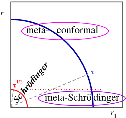
Figure 1: Spatial regions where various un-biased or biased symmetries can be realised. When distances scale isotropically with time as $r\sim\tau^{1/2}$, the time-space dynamical symmetry is the Schrödinger algebra. If a bias occurs and distances scale in the preferred direction as $r_{\|}\sim\tau$ while $r_{\perp}\sim\tau^{1/2}$ in the transverse direction, meta-Schrödinger invariance is realised. But if $r_{\|}\sim r_{\perp}\sim\tau$, meta-conformal symmetry may be realised, under certain conditions.

Table 1 summarises, besides the (ortho-)conformal algebra in $(1+1)D$, the coordinate-transformations for the infinite-dimensional conformal Galilean and Schrödinger-Virasoro groups. If applicable, an example of a Schrödinger operator on which these transformations act as dynamical symmetries, is indicated. In addition, it has been understood recently that if a directional bias occurs in the system, the dynamical symmetry can be modified [83, 84]. For example, if a bias is applied to a Schrödinger-invariant system along a preferred coordinate $r_{\|}$ and if one uses spatially anisotropic scaling such that for large distances $r_{\|},r_{\perp}\gg 1$ and large time separations $\tau\gg 1$ and keeps $r_{\|}/\tau$ and $r_{\perp}/\tau^{1/2}$ fixed, the dynamical symmetry turns into the meta-Schrödinger symmetry. However, if the scaling is made such that $r_{\|}/\tau$ and $r_{\perp}/\tau$ are kept fixed, and certain conditions on sufficiently long-ranged initial correlators are met, one may rather obtain the meta-conformal dynamical symmetry. This is illustrated in figure 1, where the domains of meta-Schrödinger and meta-conformal symmetries are indicated. Both only occur at considerably larger spatial separations than Schrödinger symmetry. This has been checked through exact calculations in the biased Glauber-Ising and spherical models [83, 126].

Applications of local scale-invariance in the context of dynamics far from equilibrium and physical ageing will be discussed in section 10.

8 Conformal Galilean Algebra

Since Lorentz and Einstein it is well-known that the Galilei group can be obtained from a contraction of the Poincaré group, in the non-relativistic limit when the speed of light $c\to\infty$. Can one obtain the Schrödinger group analogously from a contraction of the conformal group ? The question was apparently raised first by Barut [67] who stated that

The Schrödinger group [arises] from the conformal group by a combined process of contraction and a ’transfer’ of the transformation of mass to the co-ordinates.

but he does not define what he means by ‘transfer’. Since this idea is very interesting, we shall give a mathematically clean presentation of the argument, but shall also find that the meaning of ‘conformal group’ suffers a slight modification and that in the non-relativistic limit one obtains an algebra different from the Schrödinger algebra. We shall follow the presentation given in [93].

As Barut [67], we begin with the massive Klein-Gordon equation

$$\left(\frac{1}{c^{2}}\frac{\partial^{2}}{\partial t^{2}}+\frac{\partial}{\partial\bm{r}}\cdot\frac{\partial}{\partial\bm{r}}-{\cal M}^{2}c^{2}\right)\varphi(t,\bm{r})=0$$ (8.83)

Barut now attempted a change of variables via $\partial_{t}\mapsto{\cal M}c+\frac{1}{c}\partial_{t}$ but is forced to an ill-defined ‘transfer’. To implement his idea, we admit the mass $\cal M$ as a further variable [127] such that $\varphi=\varphi_{\cal M}(t,\bm{r})$ and then define a new wave function $\chi$ via

$$\varphi_{\cal M}(t,\bm{r})=\frac{1}{\sqrt{2\pi\,}\,}\int_{\mathbb{R}}\!{\rm d}u\>e^{-{\rm i}u{\cal M}}\chi(u,t,\bm{r})$$ (8.84)

which requires as a necessary condition that $\lim_{u\to\pm\infty}\chi(u,t,\bm{r})=0$. Then eq. (8.83) becomes

$$\left(\frac{1}{c^{2}}\frac{\partial^{2}}{\partial t^{2}}+\frac{\partial}{\partial\bm{r}}\cdot\frac{\partial}{\partial\bm{r}}+c^{2}\frac{\partial^{2}}{\partial u^{2}}\right)\chi(u,t,\bm{r})=0$$ (8.85)

which is a massless Klein-Gordon equation in $d+2$ dimensions (and not a massive Klein-Gordon equation in $d+1$ time-space dimensions). In the new coordinates $\xi_{-1}=\frac{u}{c},\xi_{0}=ct$ and $\xi_{j}=r_{j}$ with $j=1,\ldots,d$ and $\Psi(\bm{\xi})=\chi(u,t,\bm{r})$, eq. (8.85) becomes $\partial_{\mu}\partial^{\mu}\Psi(\bm{\xi})=0$. Its dynamical symmetry is the conformal group in its usual form, with generators

$$P_{\mu} = \partial_{\mu}$$

$$M_{\mu\nu} = \xi_{\mu}\partial_{\nu}-\xi_{\nu}\partial_{\mu}$$

$$K_{\mu} = 2\xi_{\mu}\xi^{\nu}\partial_{\nu}-\xi_{\nu}\xi^{\nu}\partial_{\mu}+2x\xi_{\mu}$$ (8.86)

$${\cal D} = \xi^{\nu}\partial_{\nu}+x$$

with summation convention over repeated indices $\mu,\nu=-1,0,1,\ldots,d$ and the scaling dimension $x$. To prepare the contraction, let

$$\psi(\zeta,t,\bm{r})=\chi(u,t,\bm{r})\mbox{\rm~{}~{}~{}where~{}~{}~{}}\zeta=u+{\rm i}c^{2}t$$ (8.87)

which we believe is the sort of ‘transfer’ Barut might have had in mind. Finally, to take the non-relativistic limit rewrite (8.85) as follows

$$\left(2{\rm i}\frac{\partial^{2}}{\partial\zeta\partial t}+\frac{\partial}{\partial\bm{r}}\cdot\frac{\partial}{\partial\bm{r}}\right)\psi(\zeta,t,\bm{r})=\frac{1}{c^{2}}\frac{\partial^{2}}{\partial t^{2}}\psi(\zeta,t,\bm{r})={\rm O}\bigl{(}c^{-2}\bigr{)}$$ (8.88)

which reduces to the free Schrödinger equation in the $c\to\infty$ limit. It remains to write the generators (8.86) in this limit, which we do here for $d=1$ for simplicity. We find (and use the notations of table 2 and figure 2).

$$\begin{array}[]{lll}P_{-1}\Psi=-{\rm i}cM\psi&P_{0}\Psi=cM\psi+{\rm O}\bigl{(}c^{-1}\bigr{)}&P_{1}\Psi=-P\psi\\ M_{01}\Psi=-cB\psi+{\rm O}\bigl{(}c^{-1}\bigr{)}&M_{-11}\Psi={\rm i}cB\psi+{\rm O}\bigl{(}c^{-1}\bigr{)}&M_{-10}\Psi={\rm i}N\psi+{\rm O}\bigl{(}c^{-2}\bigr{)}\\ K_{-1}\Psi=2{\rm i}cK\psi+{\rm O}\bigl{(}c^{-1}\bigr{)}&K_{0}\Psi=-2cK\psi+{\rm O}\bigl{(}c^{-1}\bigr{)}&K_{1}\Psi=-V_{+}\psi+{\rm O}\bigl{(}c^{-2}\bigr{)}\end{array}$$ (8.89)

for translations, rotations and expansions, respectively, while for the dilatation ${\cal D}\Psi=(-2X_{0}+N)\psi$. Herein, we used the further notations $M=P_{-1}+{\rm i}P_{0}=\frac{1}{c}\partial_{t}$, $N=-{\rm i}M_{-10}=\zeta\partial_{\zeta}-t\partial_{t}$ and $V_{+}=-\big{(}{\rm i}/2\bigr{)}^{1/2}K_{1}$. The generators of the Schrödinger algebra are given in table 2.

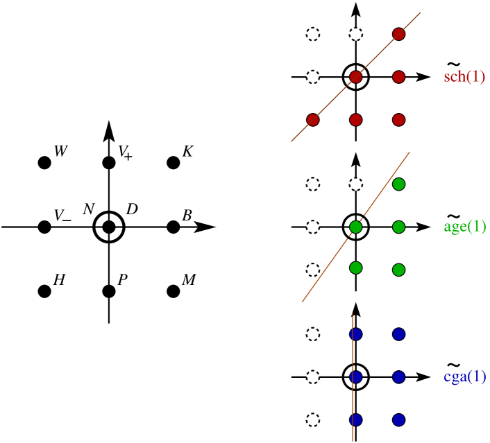
Figure 2: Left: Root diagramme of the complex Lie algebra $B_{2}$, with the generators $H,P,M,D,B,K$ of table 2 and the four additional ones $V_{\pm},W,N$. Right: the three minimal standard parabolic sub-algebras $\widetilde{\mathfrak{sch}}(1)=\mathfrak{sch}(1)\oplus\mathbb{C}N$, $\widetilde{\mathfrak{age}}(1)=\mathfrak{age}(1)\oplus\mathbb{C}N$ and $\widetilde{\mbox{\sc cga}}(1)=\mbox{\sc cga}(1)\oplus\mathbb{C}N$.

In order to understand the meaning of these result we give in figure 2, via a root diagramme, an overview of the commutator relations of the conformal algebra in $(1+1+1)$ dimensions, which is isomorphic to the complex Lie algebra $B_{2}$ [128]. This illustrates that each generator $\mathscr{X}\in B_{2}$ can be linked to a root vector $\mathfrak{x}$. For clarity, we repeat on the right of figure 2 the root diagramme for the Schrödinger algebra $\widetilde{\mathfrak{sch}}(1)=\mathfrak{sch}(1)\oplus\mathbb{C}N$. Now, the contraction procedure (8.89) leads to a different algebra, called $\mbox{\sc cga}(1)$, whose root diagramme is also indicated on the right of figure 2. Therefore, we have in the non-relativistic limit a projection [93]

$$B_{2}\cong\mathfrak{conf}(3)\to\mbox{\sc cga}(1)\not\cong\mathfrak{sch}(1)$$ (8.90)

In conclusion, Barut’s insightful idea [67] indeed works, although it leads to a different result than expected.

Figure 2 contains more information. Recall from the representation theory of Lie algebras [128] that a minimal standard parabolic sub-algebra is spanned by the Cartan sub-algebra $\mathfrak{h}$ and all positive roots of a complex semi-simple Lie algebra. In figure 2, positive roots are all roots with lie to the right of a straight line (brown) going through the origin, where the Cartan sub-algebra $\mathfrak{h}$ lies. A formal classification of the minimal standard parabolic sub-algebras of $B_{2}$ is given in [93]. The result is shown in figure 2, where the (brown) straight line can have three essentially different slopes and leads to the follows parabolic sub-algebras (up to isomorphisms generated by the transformations of the Weyl group of $B_{2}$)

$$\left\{\begin{array}[]{ll}\widetilde{\mathfrak{sch}}(1)=\mathfrak{sch}(1)\oplus\mathbb{C}N&\mbox{\rm\small Schr\"{o}dinger algebra}\\ \widetilde{\mathfrak{age}}(1)=\mathfrak{age}(1)\oplus\mathbb{C}N&\mbox{\rm\small ageing algebra}\\ \widetilde{\mbox{\sc cga}}(1)=\mbox{\sc cga}(1)\oplus\mathbb{C}N&\mbox{\rm\small conformal galilean algebra}\end{array}\right.$$ (8.91)

This should be compared with the algebras of time-space transformations constructed in section 7. There, it was seen that both the Schrödinger algebra $\mathfrak{sch}(d)$ and the conformal galilean algebra $\mbox{\sc cga}(d)$ may arise either from a study of possible time-space transformations respecting scale-invariance or else from the admissible form of geodesic curves. We now see that these two algebras are also the two main parabolic sub-algebras of the complex conformal Lie algebra $B_{2}$.

The relationship of the conformal galilean algebra with either ortho- or meta-conformal algebras may be illustrated in yet a different way. In $(1+1)$ time-space dimensions (using a more systematic notation of generators in analogy with table 2 for the Schrödinger algebra) one has for the ortho- and meta-conformal algebras, respectively, the commutators (with $n,n^{\prime}\in\mathbb{Z}$)

$$\left[X_{n},X_{n^{\prime}}\right]=(n-n^{\prime})X_{n+n^{\prime}}\;\;,\;\;\left[X_{n},Y_{n^{\prime}}\right]=(n-n^{\prime})Y_{n+n^{\prime}}\;\;,\;\;\left[Y_{n},Y_{n^{\prime}}\right]=-\mu\,(n-n^{\prime})X_{n+n^{\prime}}$$ (8.92a)

$$\left[X_{n},X_{n^{\prime}}\right]=(n-n^{\prime})X_{n+n^{\prime}}\;\;,\;\;\left[X_{n},Y_{n^{\prime}}\right]=(n-n^{\prime})Y_{n+n^{\prime}}\;\;,\;\;\left[Y_{n},Y_{n^{\prime}}\right]=\mu\,(n-n^{\prime})Y_{n+n^{\prime}}$$ (8.92b)

where $\mu=1/c$ is related to the speed of light [83]. The Lie algebra contractions now simply arises in the $\mu\to 0$ limit which give from (8.92) the commutators

$$\left[X_{n},X_{n^{\prime}}\right]=(n-n^{\prime})X_{n+n^{\prime}}\;\;,\;\;\left[X_{n},Y_{n^{\prime}}\right]=(n-n^{\prime})Y_{n+n^{\prime}}\;\;,\;\;\left[Y_{n},Y_{n^{\prime}}\right]=0$$ (8.93)

of the conformal galilean algebra $\mbox{\sc cga}(1)$. The forms (8.92) suggests the possibility of an infinite-dimensional extension, which however is possible for the ortho-conformal algebra (8.92a) in $(1+1)$ dimensions only and for the meta-conformal algebra (8.92b) in $(1+1)$ and $(1+2)$ dimensions. On the other hand, the conformal galilean algebra not only can be written for any space dimension $d$ but can always be extended to an infinite-dimensional algebra with $n,n^{\prime}\in\mathbb{Z}$. An explicit space-time representation of the conformal galilean generators in $(1+d)$ dimensions is (with $\bm{r}=\bigl{(}r_{1},\ldots,r_{d}\bigr{)}$)

$$X_{n} = -t^{n+1}\partial_{t}-(n+1)t^{n}\bm{r}\cdot\bm{\partial}-x(n+1)t^{n}-n(n+1)t^{n-1}\bm{\gamma}\cdot\bm{r}$$

$$Y_{n}^{(j)} = -t^{n+1}\partial_{j}-(n+1)t^{n}\gamma_{j}$$ (8.94)

$$R_{0}^{(jk)} = -\bigl{(}r_{j}\partial_{k}-r_{k}\partial_{j}\bigr{)}-\bigl{(}\gamma_{j}\partial_{\gamma_{k}}-\gamma_{k}\partial_{\gamma_{j}}\bigr{)};\qquad j\neq k$$

with $\partial_{j}=\frac{\partial}{\partial r_{j}}$, $x$ is a scaling dimension, the spatial rotation generators were included and we also wrote the terms coming from the rapidities $\gamma_{j}$, $j=1,\ldots,d$. In $(1+1)$ dimensions, the maximal finite-dimensional sub-algebra is $\left\langle X_{\pm 1,0},Y_{\pm 1,0}\right\rangle=\left\langle V_{+},D,P,K,B,M\right\rangle$, see also figure 2.

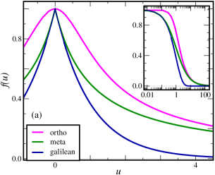
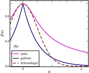
Figure 3: (a) Scaling function $f(u)$ of the covariant two-point correlator ${C}(t,r)=t^{-2x_{1}}f(r/t)$, over against the scaling variable $u=r/t$, for the ortho-conformal, meta-conformal and conformal galilean algebras, in $(1+1)D$, from eq. (8.95). The inset further underlines the different behaviour for $u\ll 1$ and $u\gg 1$. (b) Comparison with the scaling function obtained from Schrödinger-invariance, clearly distinct from both ortho-conformal and conformal galilean invariance.

The physical difference of these three algebras is further illustrated by the distinct forms of the two-point function $C(t,r)=\bigl{\langle}\phi_{1}(t,r)\phi_{2}(0,0)\bigr{\rangle}$, derived from the condition of co-variance under the maximal finite-dimensional sub-algebra $\bigl{\langle}X_{\pm 1,0},Y_{\pm 1,0}\bigr{\rangle}$ [83]

$$C(t,r)=\left\{\begin{array}[]{ll}(\bigl{(}t^{2}+\mu^{2}r^{2}\bigr{)}^{-x_{1}}\exp\bigl{(}-(2\gamma_{1}/\mu)\arctan\bigl{(}\mu|r/t|\bigr{)}\bigr{)}&\mbox{\rm\small ortho-conformal}\\ t^{-2x_{1}}\bigl{(}1+\gamma_{1}/\mu|r/t|\bigr{)}^{-2\gamma_{1}/\mu}&\mbox{\rm\small meta-conformal}\\ t^{-2x_{1}}\exp\bigl{(}-2\gamma_{1}|r/t|\bigr{)}&\mbox{\rm\small conformal galilean}\end{array}\right.$$ (8.95)

where the constraints $x_{1}=x_{2}$ and $\gamma_{1}=\gamma_{2}$ hold. In contrast with the Schrödinger algebras, which predicts co-variant response functions, the co-variant $n$-point functions found from these three algebras are correlation functions [129]. The qualitative behaviour of the associated scaling functions is shown in figure 3a. For large arguments of the scaling variable $u$, both ortho- and meta-conformal correlators decay algebraically, whereas the meta-conformal correlator has an exponential decay. On the other hand, for $u$ small, both meta-conformal and conformal galilean correlators have a pic and are not differentiable at $u=0$, whereas the ortho-conformal correlator has a rounded form. In figure 3b, the scaling functions are compared with the one obtained from Schrödinger-invariance (a response function) which clearly highlights their difference ($f(u)\sim e^{-u^{2}}$ has a gaussian form for Schrödinger-invariance).

9 Super-selection rules

We now revisit the conservation of mass. It is not simply some dynamical symmetry but has deep connections with central extensions of the time-space symmetry algebra.

1. In classical many-particle physics one may use a standard (i.e. non-projective) representation of the Galilei algebra. In an inertial frame, Newton’s equation of motion for a $N$-particle system with positions $\bm{r}_{a}(t)$ are

$$m_{a}\ddot{\bm{r}}_{a}=\bm{F}_{a}\;\;~{}~{};~{}~{}\;a=1,\ldots,N$$ (9.96)

Herein $m_{a}$ is the mass of the a^th particle and $\bm{F}_{a}$ is the force acting on it. For an isolated system, $\sum_{a=1}^{N}\bm{F}_{a}=\bm{0}$. Summing over all particles gives

$$\frac{{\rm d}}{{\rm d}t}\left(\sum_{a=1}^{N}m_{a}\dot{\bm{r}}_{a}\right)=\sum_{a=1}^{N}m_{a}\ddot{\bm{r}}_{a}=\sum_{a=1}^{N}\bm{F}_{a}=\bm{0}$$

which means that the total momentum $\bm{P}$ is conserved

$$\bm{P}=\sum_{a=1}^{N}m_{a}\dot{\bm{r}}_{a}=\mbox{\rm cste.}$$ (9.97)

such that Newton’s third axiom has been checked. In textbooks of classical mechanics this is usually derived from spatial translation-invariance. In addition to the well-known conservation law (9.97), the total mass is also conserved. To see this, change the inertial frame through a Galilei transformation

$$t\mapsto t^{\prime}=t\;\;,\;\;\bm{r}_{a}\mapsto\bm{r}_{a}^{\prime}=\bm{r}_{a}+\bm{v}t$$ (9.98)

under which (9.96) clearly is co-variant. The momentum conservation (9.97) becomes

$$\bm{P}^{\prime}=\sum_{a=1}^{N}m_{a}\dot{\bm{r}}_{a}^{\prime}=\sum_{a=1}^{N}\left(m_{a}\dot{\bm{r}}_{a}+m_{a}\bm{v}\right)=\bm{P}+\sum_{a=1}^{N}m_{a}\bm{v}$$

Since both momenta $\bm{P}$ and $\bm{P}^{\prime}$ are constant, one has the further conservation law

$$\bm{v}\sum_{a}m_{a}=\bm{P}^{\prime}-\bm{P}=\mbox{\rm cste.}~{}~{}~{}\Rightarrow~{}~{}~{}\boxed{~{}\sum_{a}m_{a}=M=\mbox{\rm cste.}~{}}$$ (9.99)

since the velocity $\bm{v}$ is arbitrary. Therefore the total mass $M$ of a non-relativistic system is always kept fixed, which is obtained here from the non-centrally extended representation (9.98). This mass conservation was established by Lavoisier more than 200 years ago, stating that [103]

“Rien ne se crée, ni dans les opérations de l’art, ni dans celles de la nature, et l’on peut poser en principe que, dans toute opération, il y a une égale quantité de matière avant et après l’opération.”

Although it is very important in practise, mass conservation appears here as a circumstantial result, found as a by-product of momentum conservation [104].

2. This become very different when one goes over to non-relativistic quantum mechanics. For a free particle, the entire information is a contained in the wave equation $\psi(t,x)$ which obeys the wave equation (for notational simplicity in $d=1$ space dimensions)

$${\rm i}\hbar\frac{\partial\psi(t,x)}{\partial t}=-\frac{\hbar^{2}}{2m}\frac{\partial^{2}\psi(t,x)}{\partial x^{2}}$$ (9.100)

where $m$ is the mass of the particle and $\hbar$ is Planck’s constant. While this equation is clearly invariant under temporal and spatial translations, it is also invariant under the Galilei transformation

$$t\mapsto t^{\prime}=t\;\;,\;\;x\mapsto x^{\prime}=x+vt$$ (9.101)

but the wave function transforms non-trivially

$$\psi(t,x)\mapsto\psi^{\prime}(t,x)=\exp\left[\frac{{\rm i}}{\hbar}\left(mxv+\frac{1}{2}mtv^{2}\right)\right]\psi(t,x-vt)$$ (9.102)

The importance of such projective representations was pointed out by Bargmann [94]. For our purposes, it is sufficient to recall that both the wave equation (9.100) as well as the law of probability conservation

$$\frac{\partial\rho(t,x)}{\partial t}+\frac{\partial j(t,x)}{\partial x}=0$$ (9.103)

transform co-variantly under the projective representation (9.102), whenever $m\neq 0$. Herein the probability density $\rho$ and the probability current $j$ are given by

$$\rho(t,x)=\psi^{*}(t,x)\psi(t,x)\;\;,\;\;j(t,x)=\frac{\hbar}{2m{\rm i}}\left(\psi^{*}(t,x)\frac{\partial\psi(t,x)}{\partial x}-\psi(t,x)\frac{\partial\psi^{*}(t,x)}{\partial x}\right)$$

This projective effect in (9.102) cannot be eliminated through a change of variables. It also follows that for $m\neq 0$, the wave function must be complex-valued. For a better algebraic understanding, we consider the Lie algebra generator $B$, obtained for infinitesimal $v$ from, (9.102)

$$B=-t\partial_{x}-\frac{{\rm i}m}{\hbar}x\;\;,\;\;P=-\partial_{x}$$ (9.104)

along with the generator $P$ of spatial translations. These are already given by Niederer [36]. In contrast to standard representations, their commutator

$$\bigl{[}B,P\bigr{]}=-\frac{{\rm i}m}{\hbar}=:\frac{{\rm i}}{\hbar}M$$ (9.105)

does not vanish for $m\neq 0$. Since $M$ does commute with all other generators of the Galilei algebra, it provides a central extension of the (non semi-simple) Galilei algebra. The presence of a non-vanishing mass $m\neq 0$ modifies profoundly the underlying mathematical structure.

3. Mass conservation can be seen as a consequence of the central extension and takes a particularly interesting form in many-body systems. When applying spatial translation-invariance and Galilei-invariance, in the form of the co-variance conditions $PC^{[n]}=BC^{[n]}=0$ with a $n$-point function $C^{[n]}=C(t_{1},\ldots,t_{n};x_{1},\ldots,x_{n})$, we find first the reduction

$$C^{[n]}=C\bigl{(}t_{1},\ldots,t_{n};x_{1}-x_{n},x_{2}-x_{n},\ldots,x_{n-1}-x_{n}\bigr{)}$$

and furthermore

$$BC^{[n]} = \left[-(t_{1}-t_{n})\partial_{x_{1}}-\ldots-(t_{n-1}-t_{n})\partial_{x_{n-1}}-\frac{{\rm i}}{\hbar}\bigl{(}m_{1}(x_{1}-x_{n})+\ldots+m_{n-1}(x_{n-1}-x_{n})\bigr{)}\right.$$

$$\left.-\frac{{\rm i}}{\hbar}x_{n}\bigl{(}m_{1}+m_{2}+\ldots+m_{n}\bigr{)}\right]C^{[n]}=0$$

Again because of spatial translation-invariance, the correlator $C^{[n]}$ only depends on the differences $x_{1}-x_{n}$, …, $x_{n-1}-x_{n}$ but cannot depend on $x_{n}$ alone. Hence one must have

$$\boxed{~{}\bigl{(}m_{1}+m_{2}+\ldots+m_{n}\bigr{)}C^{[n]}=0~{}}$$ (9.106)

This a modern rephrasing of Bargmann’s result [94]: a theory which is spatially translation-invariant and Galilei-invariant decomposes into sectors, each with a fixed mass, such that any $n$-point functions between these sectors vanish. Since it is a stronger constraint than usual selection rules from internal symmetries, it is usually called the Bargmann super-selection rule. Because of (9.102), the complex conjugate $\psi^{*}$ has a negative mass $m^{*}=-m<0$ such that the condition (9.106) can indeed be satisfied. From the present point of view, mass conservation is a fundamental property of a Galilean-invariant theory, rather than a circumstantial by-product.

4. When studying relaxational phenomena, the field-theoretic descriptions only involve real-valued fields. Certainly, this does not mean that such theories cannot be Galilei-invariant, but the notion of ‘complex conjugate’ has to be adapted. Indeed, in non-equilibrium field theory [133, 134], besides the real-valued order-parameter field $\phi$ one considers another real-valued field, the response field $\widetilde{\phi}$. In such theories, averages are calculated from functional integrals $\langle A\rangle=\int\!{\cal D}\phi{\cal D}\widetilde{\phi}\>A(\phi,\widetilde{\phi})e^{-{\cal J}[\phi,\widetilde{\phi}]}$. For a free particle at temperature $T$, the action reads

$${\cal J}[\phi,\widetilde{\phi}]=\int\!{\rm d}t{\rm d}\bm{r}\>\left[\widetilde{\phi}\bigl{(}\partial_{t}-\Delta_{\bm{r}}\bigr{)}\phi-T\widetilde{\phi}^{2}\right]$$ (9.107)

Here the response field acts as ‘complex conjugate’. If the order parameter $\phi$ has a mass $M>0$, the conjugate response field must have a mass $\widetilde{M}=-M<0$. For $N$-particle observables, each field $\phi_{j}$ of mass $M_{j}$, the generators of spatial translations and Galilei transformations can be written as (with $m=\pm\frac{1}{2}$, see table 2)

$$Y_{m}=\sum_{j=1}^{N}\left[-t_{j}^{m+1/2}\frac{\partial}{\partial x_{j}}-\left(m+\frac{1}{2}\right)M_{j}t_{j}^{m-1/2}x_{j}\right]$$ (9.108)

such that their commutator is

$$\bigl{[}Y_{1/2},Y_{-1/2}\bigr{]}=-\bigl{(}M_{1}+\ldots+M_{n}\bigr{)}=:M$$ (9.109)

We recognise the central extension by the generator $M$ and also read off the Bargmann super-selection rule $M_{1}+\ldots+M_{n}=0$. This means that averages such as $\langle\phi\widetilde{\phi}\rangle$, $\langle\phi^{2}\widetilde{\phi}^{2}\rangle$ and so on can be fixed from their co-variance. This will be explained further in section 10.

5. For comparison, we briefly reconsider the same question for the conformal Galilean algebra. A contrario to the standard galilean algebra, accelerations are also present [135]. For an $n$-particle system, the galilean generators are now (with $m=\pm 1,0$)

$$Y_{m}=\sum_{j=1}^{n}\left(-t_{j}^{m+1}\frac{\partial}{\partial x_{j}}-(m+1)\gamma_{j}t_{j}^{m}\right)$$ (9.110)

We compare the root diagrammes in figure 2. The standard galilean algebra is spanned by $\langle B,P,M\rangle\stackrel{{\scriptstyle\wedge}}{{=}}\langle Y_{\frac{1}{2}},Y_{-\frac{1}{2}},M\rangle$, see eq. (9.108), where the central extension $M$ was already included. But the space-transformations of the conformal galilean algebra are spanned by $\langle K,B,M\rangle\stackrel{{\scriptstyle\wedge}}{{=}}\langle Y_{1},Y_{0},Y_{-1}\rangle$ as given by (9.110). Therefore it is clear from figure 2 (or eq. (9.110)) that $\bigl{[}Y_{m},Y_{m^{\prime}}\bigr{]}=0$ and no central extension exists in this case. For the two-point function $C^{[2]}$, it can be easily shown, from the co-variance conditions $Y_{m}C^{[2]}=0$, that the two ‘rapidities’ are equal: $\gamma_{1}=\gamma_{2}$ [121, 136, 137]. Hence the physical rôle of the ‘masses’ $M_{j}$ and the ‘rapidities’ $\gamma_{j}$ is different. See figure 3 for the comparison of the forms of the two-point scaling functions, according to ortho-conformal, meta-conformal, conformal galilean and Schrödinger invariance.

10 Physical ageing

Galilei-invariance and the Bargmann super-selection rules find a direct application in the context of physical ageing far from equilibrium. Physical ageing is a typical behaviour of glasses [138, 139]. Here we shall be exclusively interested in the dynamical symmetry principles which are best explained in the ageing of more simple magnetic systems, without disorder [140, 141, 121].

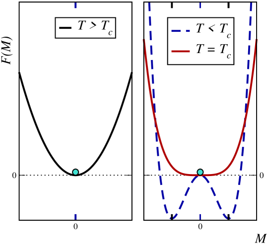
Figure 4: Schematic free energy before a quench (left panel) and after a quench to either $T=T_{c}$ or $T<T_{c}$ (right panel). The state of the system is symbolised by the small ball.

Consider a many-body system whose equilibrium state is either critical (with dynamically created long-range correlations) or else has more than one distinct but equivalent equilibrium states. Roughly speaking, physical ageing arises when the time-evolution starts from an initial state which is different from the equilibrium state. For example, one might obtain this situation via quenching a system from a fully disordered initial state to a state either onto or else below a critical temperature $T_{c}>0$, see figure 4. After the quench, the system is far from equilibrium, since it is no longer at a stable minimum of the free energy. Ageing can be monitored through the correlations of the time-space-dependent order-parameter $\phi(t,\bm{r})$. One measures for instance the single-time correlator or the two-time auto-correlator

$$C(t,\bm{r})=\left\langle\phi(t,\bm{r})\phi(t,\bm{0})\right\rangle\;\;,\;\;C(t,s)=\left\langle\phi(t,\bm{0})\phi(s,\bm{0})\right\rangle$$ (10.111)

where the averages $\bigl{\langle}\cdot\bigr{\rangle}$ are over sample histories (and possibly over an ensemble of initial conditions as well) and for simplicity spatial translation-invariance was assumed. The initial average order-parameter $\left\langle\phi(0,\bm{r})\right\rangle=0$ is taken to vanish. By definition, physical ageing occurs if the following three defining conditions are satisfied [121]

1. slow relaxational dynamics, not described by a simple exponential with a finite relaxation time

2. breaking of time-translation-invariance

3. dynamical scaling

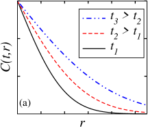
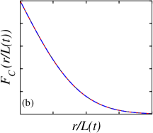
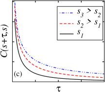
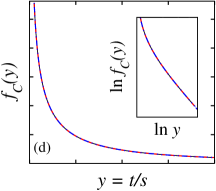
Figure 5: Illustration of the characteristic data collapse of physical ageing. Panel (a) shows a typical behaviour of a single-time correlator for different times $t_{3}>t_{2}>t_{1}$, while (b) shows the collapse onto a single curve when distances $r=|\bm{r}|$ are measured in units of the dynamical length scale $L(t)$. Panel (c) similarly illustrates the two-time autocorrelator in dependence of $\tau=t-s$, for different waiting times $s_{1}<s_{2}<s_{3}$ and panel (d) shows that these data collapse when replotted as a function of $y=t/s$. The log-log plot in the inset shows the asymptotic power-law form $f_{C}(y)\sim y^{-\lambda/z}$.

Figure 5 schematically illustrates how ageing can be detected from correlation functions. The curves of $C(t,\bm{r})$ do depend on time, hence there is no time-translation-invariance. But if the same data are replotted over against $\bigl{|}\bm{r}\bigr{|}/L(t)$, where $L(t)\sim t^{1/z}$ is the time-dependent length of the ordered clusters, ($z$ is the dynamical critical exponent) a data collapse occurs. Similarly, the curves of the two-time autocorrelator $C(t,s)$, when plotted over against the time difference $\tau=t-s$, do depend on the waiting time $s$ and time-translation-invariance is broken. Again, when replotted over against $y=t/s$, a data collapse occurs. Hence in the limit of large times, one finds the scaling forms

$$C(t,\bm{r})=t^{-c}F_{C}\left(\frac{\bm{r}}{L(t)}\right)\;\;,\;\;C(t,s)=s^{-b}f_{C}\left(\frac{t}{s}\right)$$ (10.112)

The inset in figure 5d illustrates the generic power-law behaviour of $f_{C}(y)\sim y^{-\lambda/z}$ for $y\gg 1$ large. The auto-correlation exponent $\lambda$ is universal but for a non-conserved order-parameter it is independent of all equilibrium critical exponents [142]. The renormalisation group asserts that scaling functions such as $F_{C}$ and $f_{C}$ are universal. Then their functional from should only depend on global system properties such as dimension and global symmetries but should be independent of most microscopic ‘details’ of a specific hamiltonian. Finding their form, independently of studies in specific models, then calls for a convenient dynamical symmetry.

Probably the most simple system with a dynamical exponent $z=2$ is the Edwards-Wilkinson model, see [143], for the height $h=h(t,\bm{r})$ of a growing interface. In a frame where the average height is constant, $\partial_{t}\langle h(t,\bm{r})\rangle=0$, the height fluctuations are described by the Langevin equation

$$\partial_{t}h(t,\bm{r})=\frac{1}{2\cal M}\Delta_{\bm{r}}h(t,\bm{r})+\eta(t,\bm{r})$$ (10.113)

where $\Delta_{\bm{r}}$ is the spatial laplacian and fluctuations enter through the centred gaussian white noise with variance $\left\langle\eta(t,\bm{r})\eta(t^{\prime},\bm{r}^{\prime})\right\rangle=2T{\cal M}\delta(t-t^{\prime})\delta(\bm{r}-\bm{r}^{\prime})$. Following [144], we shall use this simple model, with its linear Langevin equation, to illustrate some of the main aspects of dynamical Schrödinger symmetry. Clearly, the noise term in (10.113) breaks any time-space symmetry beyond simple translation- and rotation-invariance. Hence the noisy eq. (10.113), as it stands, cannot be Schrödinger-invariant.

Eq. (10.113) can be obtained as a classical equation of motion of the non-equilibrium Janssen-de Dominicis field theory [133, 134, 142], with the action ${\cal J}[h,\widetilde{h}]={\cal J}_{0}[h,\widetilde{h}]+{\cal J}_{b}[\widetilde{h}]$ decomposed into a deterministic and a noise part, respectively

$${\cal J}_{0}[h,\widetilde{h}] = \int\!{\rm d}t{\rm d}\bm{r}\>\widetilde{h}\bigl{(}\partial_{t}-(2{\cal M})^{-1}\Delta_{\bm{r}}-j\bigr{)}h$$

$${\cal J}_{b}[\widetilde{h}] = -T\int\!{\rm d}t{\rm d}\bm{r}\>\widetilde{h}^{2}$$ (10.114)

Herein, $\widetilde{h}$ is the response field conjugate to the height field $h$. Averages are computed from the functional integral $\langle\mathscr{A}\rangle=\int{\cal D}h{\cal D}\widetilde{h}\;\mathscr{A}[h]e^{-{\cal J}[h,\widetilde{h}]}$. Notably, one distinguishes two-particle correlation and response functions [140, 121, 142],

$$C(t_{1},t_{2};\bm{r}_{1},\bm{r}_{2}) =\biggl{\langle}h(t_{1},\bm{r}_{1})h(t_{2},\bm{r}_{2})\biggr{\rangle}$$ (10.115a)

$$R(t_{1},t_{2};\bm{r}_{1},\bm{r}_{2}) =\left.\frac{\delta\langle h(t_{1},\bm{r}_{1})}{\delta j(t_{2},\bm{r}_{2})}\right|_{j=0}=\left\langle h(t_{1},\bm{r}_{1})\widetilde{h}(t_{2},\bm{r}_{2})\right\rangle$$ (10.115b)

which explains the purpose of the source field $j$ in eq. (10.114) and the name of the response field $\widetilde{h}$.

Now, the deterministic part ${\cal J}_{0}[h,\widetilde{h}]$ of the action is Schrödinger-invariant (related to the heat equation). This allows us to identify the following properties of the height field $h$ and its conjugate response field $\widetilde{h}$:

height field $h$ :	scaling dimension $x$	mass ${\cal M}>0$
response field $\widetilde{h}$ :	scaling dimension $\widetilde{x}$	mass $\widetilde{\cal M}=-{\cal M}<0$

It follows from the Bargmann super-selection rules that the $(n+m)$-point deterministic correlator, computed only with the part ${\cal J}_{0}[h,\widetilde{h}]$ of the action, obeys

$$C^{[n,m]}_{0}=\left\langle h_{1}\ldots h_{n}\widetilde{h}_{1}\ldots\widetilde{h}_{m}\right\rangle_{0}=\delta_{n,m}\mathscr{C}^{[n]}$$ (10.116)

such that only deterministic averages with an equal number of $h$- and $\widetilde{h}$-fields can be non-vanishing. A non-trivial example would be the response function $R=C^{[1,1]}$, see (10.115b). However, the deterministic correlator $C=C^{[2,0]}_{0}=0$ vanishes. A formal expansion [145] in the full action in terms of the ‘temperature’ $T$ then shows from (10.115b) that the (noisy) response function $R=\langle h\widetilde{h}\rangle$

$$R(t,s;\bm{r})=\left\langle h(t,\bm{r})\widetilde{h}(s,\bm{0})e^{-{\cal J}_{b}[\widetilde{h}]}\right\rangle_{0}=\left\langle h(t,\bm{r})\widetilde{h}(s,\bm{0})\right\rangle_{0}=R_{0}(t,s;\bm{r})$$ (10.117)

which is computed in a stochastic model, is identical to the deterministic response $R_{0}$ found from Schrödinger-invariance. Similarly the correlator $C=\langle hh\rangle$

$$C(t,s;\bm{r})=\left\langle h(t,\bm{r}){h}(s,\bm{0})e^{-{\cal J}_{b}[\widetilde{h}]}\right\rangle_{0}=T\int\!{\rm d}u{\rm d}\bm{R}\>\left\langle h(t,\bm{r}){h}(s,\bm{0})\widetilde{h}^{2}(u,\bm{R})\right\rangle_{0}$$ (10.118)

reduces to an integral of a deterministic three-point response function [145]. The exact reduction formulæ (10.117,10.118) are the basis for finding the scaling functions of responses and correlators.

We note an important feature of Schrödinger-invariance: the requirement of co-variance fixes directly response functions, such as $R=\bigl{\langle}h\widetilde{h}\bigr{\rangle}$, because they are compatible with the Bargmann super-selection rule (10.116). On the other hand, a co-variance requirement imposed on a correlation function, such as $C=\bigl{\langle}hh\bigr{\rangle}$, would force it to vanish, because the Bargmann super-selection rule (10.116) cannot be satisfied. Correlators will always be obtained by reducing them to higher response functions [145]. The causality of response functions can be systematically derived from a detailed analysis of the time-space representations [93, 129].

After these preparations, we finally return to the example of the Edwards-Wilkinson model, described by the Langevin equation (10.113). It is enough to find the two- and three-point response function of the deterministic theory, from the co-variance under the generators of the Schrödinger Lie algebra. First, with (10.117), the two-time response function is [60] (with $t>s$ because of causality [93])

$$R(t,s;\bm{r})=r_{0}\delta_{x,\widetilde{x}}\delta({\cal M}+\widetilde{\cal M})(t-s)^{-x}\exp\left[-\frac{\cal M}{2}\frac{\bm{r}^{2}}{t-s}\right]$$ (10.119)

The constraint $x=\widetilde{x}$ is analogous to the one following from conformal invariance. In addition, the masses ${\cal M}=-\widetilde{\cal M}>0$ are related by the Bargmann rule. These two conditions express the relationship of the field $h$ and its conjugate response field $\widetilde{h}$. Second, we find the single-time correlator $C(t,\bm{r})$ with (10.118). We need the generic three-point response [60] (for $\varepsilon\to 0$ and with $t>u$ because of causality [93])

$$\left\langle h(t+\varepsilon,\bm{r}+\bm{r}_{0})h(t,\bm{r}_{0}){\widetilde{h}}^{2}(u,\bm{R})\right\rangle_{0}=\delta(2{\cal M}+2\widetilde{\cal M})$$ (10.120)

$$\times (t+\varepsilon-u)^{-x}(t-u)^{-x}\exp\left[-\frac{\cal M}{2}\frac{(\bm{r}+\bm{r}_{0}-\bm{R})^{2}}{t+\varepsilon-u}-\frac{\cal M}{2}\frac{(\bm{r}_{0}-\bm{R})^{2}}{t-u}\right]$$

$$\times \Psi\left(\frac{\bigl{(}(\bm{r}+\bm{r}_{0}-\bm{R})(t-u)-(\bm{r}_{0}-\bm{R})(t+\varepsilon-u)\bigr{)}^{2}}{(t+\varepsilon-u)(t-u)\varepsilon}\right)$$

where we already used $x_{{\widetilde{h}}^{2}}=2\widetilde{x}$ and $\widetilde{x}=x$. In the limit $\varepsilon\to 0$ this must be finite such that the unknown scaling function $\Psi$ reduces to a constant $\Psi_{0}$. We find

$$C(t,\bm{r}) = T\Psi_{0}\int_{0}^{t}\!{\rm d}u\>u^{-2{x}}\int_{\mathbb{R}^{d}}\!{\rm d}\bm{R}\>\exp\left[-\frac{\cal M}{2u}\left[\left(\frac{\bm{r}}{2}-\bm{R}\right)^{2}+\left(\frac{\bm{r}}{2}+\bm{R}\right)^{2}\right]\right]$$ (10.121)

$$= {T\Psi_{0}}\left(\frac{\pi}{\cal M}\right)^{d/2}\int_{0}^{t}\!{\rm d}u\>u^{d/2-2{x}}\exp\left[-\frac{\cal M}{4}\frac{\bm{r}^{2}}{u}\right]$$

$$= T{c}_{0}\>|\bm{r}|^{d+2-4x}\,\Gamma\left(2{x}-\frac{d}{2}-1,\frac{\cal M}{4}\frac{\bm{r}^{2}}{t}\right)$$

where $\Psi_{0}$ and $c_{0}$ are normalisation constants and $\Gamma$ is an incomplete Gamma function. It clearly appears that $C(t,\bm{r})$ is determined by the fluctuations in $h$ which in turn come from the noise in (10.113). But we also had to rely on consistency arguments, based on scaling, in order to fix the unknown function $\Psi$ which is not determined by Schrödinger-invariance alone.

The predictions (10.119) and (10.121) can now be compared with the exact results of the Edwards-Wilkinson model, readily obtained by solving (10.113) [146]. If one identifies $x=d/2$, and matches the non-universal mass $\cal M$, the agreement is perfect [144]. This simple example illustrates the idea how the scaling dimension $x$ of the quasi-primary field of the Schrödinger group determines the functional form of the universal scaling function $F_{C}$ of the single-time correlator. Two-time correlators can be treated analogously [146].

We close with a few further comments.
1. When quenching a magnetic system to below $T_{c}>0$, and the order-parameter is not conserved, the system undergoes phase-ordering kinetics, with a dynamical exponent $z=2$ always [147, 148]. However, the representations of the Schrödinger group with generators ${\cal X}^{\rm equ}$ must be replaced by [84, 126]

$${\cal X}^{\rm equ}\mapsto{\cal X}=e^{\xi\ln t}{\cal X}^{\rm equ}e^{-\xi\ln t}$$ (10.122)

where the generators ${\cal X}^{\rm equ}$ are those listed in table 2. Herein, $\xi$ serves as a further quantum number of the scaling operator these generators act on. In this setting, one is not obliged to simply drop the time-translation generator $X_{-1}$ from the algebra. Rather, the breaking of time-translation-invariance occurs ‘softly’, since one now has

$$X_{-1}^{\rm equ}\mapsto X_{-1}=e^{\xi\ln t}\bigl{(}-\partial_{t}\bigr{)}e^{-\xi\ln t}=-\partial_{t}+\frac{\xi}{t}$$ (10.123)

which explicitly depends on time. This construction holds true for the entire Schrödinger-Virasoro algebra [149]. In the representation (10.122), the Schrödinger operator also becomes time-dependent, for example

$$\mathscr{S}^{\rm equ}\mapsto\mathscr{S}=e^{\xi\ln t}\left(\partial_{t}-\partial_{r}^{2}\right)e^{-\xi\ln t}=\partial_{t}+\frac{\xi}{t}-\partial_{r}^{2}$$ (10.124)

This reproduces simulations in many models of phase-ordering, see [121].
2. For a critical quench to $T=T_{c}$, in general the dynamic exponent $z\neq 2$. Since the form of the auto-response functions, determined from co-variance, only depends on $\lambda/z$, that part of the theory can still be used, to a good degree of precision [121, 150]. However, there are indications that a better choice of representation might be a logarithmic one – in analogy to logarithmic conformal field theory [151, 152], where the scaling operators become at least two-component vectors and the scaling dimensions $x$ are replaced by Jordan matrices. Such logarithmic representations have been constructed for the Schrödinger algebra [153, 154] and indeed permit a much improved agreement with simulational data of response functions in several critical models ($1D$ critical directed percolation [158], the $1D/2D$ Kardar-Parisi-Zhang equation [159, 160] and the $2D$ critical Ising model [161]).

11 Conclusions

The twin conformal and Schrödinger groups stand at the beginning of the systematic applications of continuous symmetry in physics, as initiated by Jacobi [26] and Lie [27]. The pioneering work of Brinkmann [85] and of Eisenhart [28] was followed by the introduction and comprehensive use of Duval et al.’s (“Bargmann”) framework [86]. This allowed, apart of finding all Schrödinger-symmetric mechanical systems, to study Chern-Simons vortices and fluid mechanics. As a further example then arose the conformal galilean group (and the recently identified meta-conformal and meta-Schrödinger groups), see table 1. After retracing some historical steps, and recalling several important concepts related to central extensions and super-selection rules, and whose development took insight from quite distinct areas of physics (and mathematics) we have seen that these three symmetries arise time and again in physical applications, only provided that there is a physical basis for emergent scale-invariance. An important difference of Galilei- and Schrödinger-groups on one side and relativistic or non-relativistic conformal groups on the other, are the Bargmann super-selection rules which can be traced back to central extensions in these non-semi-simple algebras. Some examples, notably physical ageing, were treated more explicitly. Through the various applications mentioned in this review we hope to have given sufficient motivation to strive further in an ever improving understanding and on the deep relations between them.

A major outcome of these symmetries are bootstrap approaches which try to achieve as much as possible for the symmetry itself. The most magnificent example remains of course the conformal bootstrap in $d=2$ spatial dimensions [8], which has led to so many consequences in either $2D$ equilibrium critical phenomena or else in string theory. It has been tried to follow these paths in different settings, notably in conformal field-theory in $d>2$ dimensions, e.g. [162, 163, 164], or conformal galilean and BMS theory, e.g. [165, 166, 167, 168].

We regret to have to resist the temptation to deal with supersymmetric extensions of Galilei- and Schrödinger-symmetry. A natural starting point would be the spin-$\frac{1}{2}$ Lévy-Leblond equation [169]. Since a discussion would require an article by itself, we limit ourselves to the mere statement that these studies were initiated in [170, 171, 172, 173, 174, 175, 176, 177].

Acknowledgements: This project was initiated jointly with Christian Duval before his untimely death. We would like to thank Gary Gibbons for his interest, advice, and his contribution at the early stages of this work. MH was supported by the french ANR UNIOPEN (ANR-22-CE30-0004-01). PMZ was partially supported by the National Natural Science Foundation of China (Grant No. 11975320).

References

- [1] H. Weyl, Symmetrie, Birkhäuser (Basel 1955).
- [2] J.D. Bjørken, “Asymptotic Sum Rules at Infinite Momentum”, Phys. Rev. 179, 1547 (1969).
- [3] G. Altarelli, G. Parisi, “Asymptotic freedom in parton language”, Nucl. Phys. B126, 298 (1977).
- [4] D.G. Boulware, L.S. Brown, R.D. Pecceci, “Deep-Inelastic Electroproduction and Conformal Symmetry”, Phys. Rev. D2, 293 (1970).
- [5] J. Polchinski, String Theory. Vol. 1: An Introduction to the Bosonic String, Cambridge Univ. Press (Cambridge 1998).
- [6] K. Becker, M. Becker, J. H. Schwarz, String theory and M-theory: A modern introduction, Cambridge Univ. Press (Cambridge 2007).
- [7] A.M. Polyakov, ‘Conformal symmetry of critical fluctuations”, Sov. Phys. JETP Lett. 12, 381 (1970).
- [8] A.A. Belavin, A.M. Polyakov, A.B. Zamolodchikov, “Infinite conformal symmetry in two-dimensional quantum field-theory”, Nucl. Phys. B241, 333 (1984).
- [9] A.B. Zamolodchikov, “Integrable Field Theory from Conformal Field Theory”, Adv. Stud. Pure Math. 19, 641 (1989).
- [10] J. Maldacena, “The Large- Limit of Superconformal Field Theories and Supergravity”, Int. J. Theor. Phys. 38, 1113 (1999), [arXiv:hep-th/9711200].
- [11] O. Aharony, S. Gubser, J. Maldacena, H. Ooguri, Y. Oz, “Large- Field Theories, String Theory and Gravity”, Phys. Rep. 323, 183 (2000). [arXiv:hep-th/9905111].
- [12] H. Bondi, M.G.J. van der Burg, A.W.K. Metzner, “Gravitational waves in general relativity”, Proc. R. Soc. Lond. A269, 21 (1962).
- [13] R.K. Sachs, “Gravitational waves in general relativity VIII. Waves in asymptotically flat space-time”, Proc. R. Soc. Lond. A270, 103 (1962).
- [14] G. Barnich and G. Compère, “Classical central extension for asymptotic symmetries at null infinity in three spacetime dimensions”, Class. Quant. Grav. 24 F15 (2007); corrigendum 24, 3139 (2007) [gr-qc/0610130].
- [15] A. Bagchi, and R. Gopakumar, “Galilean Conformal Algebras and AdS/CFT,” JHEP 0907:037 (2009), [arXiv:0902.1385 [hep-th]].
- [16] D. Martelli, Y. Tachikawa, Comments on Galilean conformal field theories and their geometric realization, JHEP 1005:091 (2010), [arXiv:0903.5184].
- [17] G. Barnich, A. Gomberoff, H.A. González, “Three-dimensional Bondi-Metzner-Sachs invariant two-dimensional field-theories as the flat limit of Liouville theory”, Phys. Rev. D87, 124032 (2007), [arxiv:1210.0731].
- [18] J.D. Miller and K De’Bell, “Randomly branched polymers and conformal invariance”, J. Physique I3, 1717 (1993).
- [19] V. Riva and J.L. Cardy, “Scale and conformal invariance in field theory: a physical counterexample”, Phys. Lett. B622, 339 (2005) [arxiv:hep-th/0504197].
- [20] A. Gimenez-Grau, Y. Nakayama, S. Rychkov, “Scale without Conformal Invariance in Dipolar Ferromagnets” [arXiv:2309.02514].
- [21] J. Polchinski, “Scale and conformal invariance in quantum field theory”, Nucl. Phys. B303, 226 (1988).
- [22] D. Dorigoni and V. S. Rychkov, “Scale Invariance + Unitarity Conformal Invariance?”, [arXiv:0910.1087 [hep-th]].
- [23] C. Duval, P. A. Horvathy and L. Palla, “Conformal Properties of Chern-Simons Vortices in External Fields,” Phys. Rev. D50, 6658 (1994) [arXiv:hep-th/9404047 [hep-th]].
- [24] C. Duval, and P. A. Horváthy “Non-relativistic conformal symmetries and Newton-Cartan structures,” J. Phys. A42, 465206 (2009) [arXiv:0904.0531 [math-ph]].
- [25] M. Henkel, “Phenomenology of local scale invariance: From conformal invariance to dynamical scaling,” Nucl. Phys. B641, 405 (2002) [arXiv:hep-th/0205256].
- [26] C.G.J. Jacobi, “Vorlesungen über Dynamik.” Univ. Königsberg 1842-43. Herausg. A. Clebsch. Vierte Vorlesung: Das Prinzip der Erhaltung der lebendigen Kraft. Zweite Ausg. C. G. J. Jacobi’s Gesammelte Werke. Supplementband. Herausg. E. Lottner. Berlin Reimer (1884). A recent english translation is available as Jacobi’s Lectures on Dynamics, 2nd edition, Texts and Readings in Mathematics, https://doi.org/10.1007/978-93-86279-62-0, Hindustan Book Agency Gurgaon.
- [27] S. Lie, “Über die Integration durch bestimmte Integrale von einer Klasse linearer partieller Differentialgleichungen,” Arch. Math. (Kristiania) 6, 328 (1881).
- [28] L. P. Eisenhart, “Dynamical trajectories and geodesics”, Ann. of Math. 30, 591 (1929).
- [29] P. Appell, “Sur l’équation et la théorie de la chaleur”, J. Mathématiques Pures Appliquées, 4e série, 8, 187 (1892).
- [30] J.A. Goff, “Transformations leaving invariant the heat equation of physics”, Amer. J. Math. 49, 117 (1927).
- [31] L.V. Ovsiannikov, “Groups and group-invariant solutions of differential equations”, Dokl. Akad. Nauk SSSR 118, 439 (1958) (in russian).
- [32] L.V. Ovsiannikov, Group analysis of differential equations, Academic Press (London 1982) – this is a translation of the russian edition from 1978.
- [33] W.I. Fushchich, W.M. Shtelen, N.I. Serov, Symmetry analysis and exact solutions of equations of non-linear mathematical physics, Kluwer (Dordrecht 1993) – this is an extended translation of the russian edition from 1989.
- [34] W.I. Fushchich, A.G. Nikitin, Symmetries of equations of quantum mechanics, Allerton Press (New York 1994)– this is an extended translation of the russian edition from 1990.
- [35] R. Jackiw, “Introducing scale symmetry”, Phys. Today 25 (1972) 23.
- [36] U. Niederer, “The maximal kinematical invariance group of the free Schrödinger equation”, Helv. Phys. Acta 45, 802 (1972).
- [37] C. R. Hagen, “Scale and conformal transformations in galilean-covariant field theory”, Phys. Rev. D5, 377 (1972).
- [38] J. M. Levy-Leblond, “Nonrelativistic particles and wave equations,” Commun. Math. Phys. 6, 286 (1967)
- [39] J. Gomis, M. Novell, “A pseudoclassical description for a nonrelativistic spinning particle. 1. The Levy-leblond Equation”, Phys. Rev. D33, 2212 (1986).
- [40] C. Duval, P. A. Horvathy and L. Palla, “Spinors in nonrelativistic Chern-Simons electrodynamics,” Ann. of Phys. 249, 265 (1996) [arXiv:hep-th/9510114 [hep-th]].
- [41] P. Roman, J. J. Aghassi, R. M. Santilli, and P. L. Huddleston, “Nonrelativistic composite elementary particles and the conformal Galilei group”, Nuovo Cim. 12, 185 (1972).
- [42] G. Burdet, and M. Perrin, “Many-body realization of the Schrödinger algebra”, Lett. Nuovo Cim. 4, 651 (1972)
- [43] G. Burdet, M. Perrin, and P. Sorba, “About the Non-Relativistic Structure of the Conformal Algebra,” Commun. Math. Phys. 34, 85 (1973).
- [44] U. Niederer, “The maximal kinematical invariance groups of Schrödinger equations with arbitrary potentials”, Helv. Phys. Acta. 47, 167 (1974).
- [45] V. de Alfaro, S. Fubini and G. Furlan, “Conformal Invariance in Quantum Mechanics,” Nuovo Cim. A34, 569 (1976)
- [46] C.P. Boyer, R.T. Sharp, P. Winternitz, “Symmetry-breaking interaction for the time-dependent Schrödinger equation”, J. Math. Phys. 17, 1439 (1976).
- [47] A.G. Nikitin, R.O. Popovych, “Group classification of non-linear Schrödinger equations”, Ukr. Math. J. 53, 1255 (2001) [arxiv:math-ph/0301009].
- [48] S. Dhasmana, A. Sen and Z. K. Silagadze, “Equivalence of a harmonic oscillator to a free particle and Eisenhart lift,” Ann. of Phys. 434, 168623 (2021), [arXiv:2106.09523 [quant-ph]].
- [49] A. Bihlo, R.O. Popovych, “Group classification of linear evolution equations”, J. Math. Anal. Appl. 448, 982 (2017) [arxiv:1605.09251].
-
[50]
R. Cherniha, J.R. King,
“Lie symmetries of nonlinear multidimensional reaction-diffusion systems: I”,
J. Phys. A: Math. Gen. 33, 267 (2000);
R. Cherniha, J.R. King, “Lie symmetries of nonlinear multidimensional reaction-diffusion systems: II”, J. Phys. A: Math. Gen. 36, 405 (20003). - [51] R. Cherniha, V. Davydovych, Nonlinear Reaction-Diffusion Systems: Conditional Symmetry, Exact Solutions and their Applications in Biology, Lecture Notes Mathematics 2196, Springer (Heidelberg 2017).
- [52] R. Jackiw, “Dynamical Symmetry of the Magnetic Monopole,” Ann. of Phys. 129, 183 (1980)
- [53] R. Jackiw, “Dynamical Symmetry of the Magnetic Vortex,” Ann. of Phys. 201, 83 (1990).
- [54] C. Duval, “Quelques procédures géométriques en dynamique des particules,” Doctoral Thesis, Marseille (1982).
- [55] R. Jackiw and S. Y. Pi, “Classical and quantal nonrelativistic Chern-Simons theory,” Phys. Rev. D42, 3500 (1990) [erratum: Phys. Rev. D48 3929 (1993)].
- [56] C. Duval, P. A. Horvathy and L. Palla, “Conformal symmetry of the coupled Chern-Simons and gauged nonlinear Schrödinger equations,” Phys. Lett. B325, 39 (1994). [arXiv:hep-th/9401065 [hep-th]].
- [57] R. Jackiw, “A Particle field theorist’s lectures on supersymmetric, non-abelian fluid mechanics and d-branes,” Lectures CRM Montréal (2000), [arXiv:physics/0010042 [physics]].
- [58] M. Hassaine and P. A. Horvathy, “Symmetries of fluid dynamics with polytropic exponent”, Phys. Lett. A279, 215 (2001) [arXiv:hep-th/0009092 [hep-th]].
- [59] P. A. Horvathy and P. M. Zhang, “Non-relativistic conformal symmetries in fluid mechanics”, Eur. Phys. J. C65 (2010), 607-614 [arXiv:0906.3594 [physics.flu-dyn]].
- [60] M. Henkel “Schrödinger invariance and strongly anisotropic critical systems,” J. Stat. Phys. 75, 1023 (1994) [arXiv:hep-th/9310081].
- [61] K. Balasubramanian, J. McGreevy, “Gravity Duals for Nonrelativistic Conformal Field Theories”, Phys. Rev. Lett. 101, 061601 (2008), [arXiv:0804.4053].
- [62] D.T. Son, “Toward an AdS/cold atoms correspondence: A geometric realization of the Schrödinger symmetry”, Phys. Rev. D78, 046003 (2008), [arXiv:0804.3972].
- [63] D. Minic, M. Pleimling, “Correspondence between nonrelativistic anti-de Sitter space and conformal field theory, and aging-gravity duality”, Phys. Rev.E78, 061108 (2008), [arXiv:0807.3665]; N. Gray, D. Minic, M. Pleimling, “On non-equilibrium physics and string theory ”, Int. J. Mod. Phys. A28, 1330009 (2013), [arXiv:1301.6368].
- [64] C.A. Fuertes, S. Moroz, “Correlation functions in the nonrelativistic AdS/CFT correspondence”, Phys. Rev.D79, 106004 (2009), [arXiv:0903.1844].
-
[65]
R.G. Leigh, N.N. Hoang,
“Real-time correlators and non-relativistic holography”,
J. High Energy Phys. 0911:010,2009
[arXiv:0904.4270];
R.G. Leigh, N.N. Hoang, “Fermions and the Sch/nrCFT Correspondence”, J. High Energy Phys. 1003:027,2010, [arxiv:0909.1883]. - [66] S. Moroz, “Nonrelativistic scale anomaly, and composite operators with complex scaling dimensions”, Ann. of Phys. 326, 1368 (2011); [arXiv:1007.4635].
-
[67]
A.O. Barut
“Conformal Group Schrödinger Group
Dynamical Group — The Maximal Kinematical
Group of the Massive Schrödinger Particle,”
Helv. Phys. Acta 46, 496 (1973);
U. Niederer, “The connections between the Schrödinger group and the conformal group,” Helv. Phys. Acta 47, 119 (1974). - [68] E. Noether, “Invariante Variationsprobleme [Invariants of variational problems],”, Nachr. Ges. Wiss. Göttingen, Math.-Phys., 1918b, p. 235-257, Gött. Nachr.1918:235-257,1918; Transp.Theory Statist. Phys.1:186-207,1971 [arXiv:physics/0503066 [physics.hist-ph]]
- [69] J.-M. Souriau Structure des systèmes dynamiques, Dunod (1970); Structure of Dynamical Systems. A Symplectic View of Physics, translated by C.H. Cushman-de Vries (R.H. Cushman and G.M. Tuynman, Translation Editors), Birkhäuser (1997).
- [70] C. Duval, G. W. Gibbons, P. A. Horvathy and P. M. Zhang, “Carroll Newton and Galilei: two dual non-Einsteinian concepts of time,” Class. Quant. Grav. 31 (2014), 085016 [arXiv:1402.0657 [gr-qc]].
- [71] J. M. Lévy-Leblond, “Une nouvelle limite non-relativiste du group de Poincaré”, Ann. Inst. H. Poincaré 3, 1 (1965).
-
[72]
R. Casalbuoni, D. Dominici and J. Gomis,
“Two interacting conformal Carroll particles,”
[arXiv:2306.02614 [hep-th]];
P. M. Zhang, H. X. Zeng and P. A. Horvathy, “MultiCarroll dynamics,” [arXiv:2306.07002 [gr-qc]]. - [73] L. Marsot, P. M. Zhang, M. Chernodub and P. A. Horvathy, “Hall effects in Carroll dynamics,” Phys. Rep. 1028, 1 (2023) [arXiv:2212.02360 [hep-th]].
- [74] J. Kepler, “Astronomia Nova”, [New Astronomy] (1609) chap.59. See https://en.wikipedia.org/wiki/Astronomia-nova # .
- [75] C. Duval, G. W. Gibbons and P. Horvathy, “Celestial mechanics, conformal structures and gravitational waves,” Phys. Rev. D43, 3907 (1991) [arXiv:hep-th/0512188].
- [76] P. A. M. Dirac, “A new basis for cosmology,” Proc. Roy. Soc. A165, 199 (1938).
- [77] U. Niederer, “The maximal kinematical invariance group of the harmonic oscillator”, Helv. Phys. Acta. 46, 192 (1973).
- [78] U. Niederer, “Schrödinger-invariant generalized heat equations”, Helv. Phys. Acta 51, 220 (1978).
- [79] L. Martina and O. K. Pashaev, “Burgers’ equation in noncommutative space-time”, in M.J. Ablowitz et al. (eds) Nonlinear physics: theory and experiment II, World Scientific (Singapour 2002) [arXiv:hep-th/0302055 [hep-th]].
- [80] E.V. Ivashkevich, “Symmetries of the stochastic Burgers equation”, J. Phys. A30, L525 (1997) [arXiv:hep-th/9610221].
- [81] P. Havas, J. Plebanski “Conformal extensions of the Galilei group and their relation to the Schrödinger group,” J. Math. Phys. 19, 482 (1978).
- [82] J. Negro, M.A. del Olmo and A. Rodríguez-Marco, “Nonrelativistic conformal groups” I & II, J. Math. Phys. 38, 3786 (1997); 38, 3810 (1997).
- [83] M. Henkel, S. Stoimenov, “Infinite-dimensional meta-conformal Lie algebras in one and two spatial dimensions”, J. Stat. Mech. 084009 (2019) [arxiv:1810.09855].
- [84] S. Stoimenov, M. Henkel, “Meta-Schrödinger-invariance”, Nucl. Phys. B985, 116020 (2022) [arxiv:2112.14143].
- [85] M. W. Brinkmann, “On Riemann spaces conformal to Euclidean spaces”, Proc. Natl. Acad. Sci. U.S. 9, 1 (1923); ‘Èinstein spaces which are mapped conformally on each other”, Math. Ann. 94, 119 (1925).
- [86] C. Duval, G. Burdet, H.P. Künzle, and M. Perrin; “Bargmannn Structures and Newton-Cartan Theory,” Phys. Rev. D31, 1841 (1985).
-
[87]
J. Gomis, J.M. Pons,
“Poincare Transformations and Galilei Transformations.”
Phys. Lett. A66 463 (1978);
J. Gomis, A. Poch, J. M. Pons, “Poincare wave equations as Fourier transforms of Galilei wave equations.” J. Math. Phys. 21 2682 (1980). - [88] H. P. Künzle, “Galilei and Lorentz structures on space-time : Comparison of the corresponding geometry and physics”, Ann. Inst. Henri Poincaré 17A, 337 (1972).
- [89] C. Duval, G. W. Gibbons, P. A. Horvathy and P. M. Zhang, “Carroll versus Newton and Galilei: two dual non-Einsteinian concepts of time,” Class. Quant. Grav. 31, 085016 (2014) [arXiv:1402.0657 [gr-qc]].
- [90] M. Elbistan, N. Dimakis, K. Andrzejewski, P. A. Horvathy, P. Kosínski and P. M. Zhang, “Conformal symmetries and integrals of the motion in pp waves with external electromagnetic fields,” Ann. of Phys. 418, 168180 (2020) [arXiv:2003.07649 [gr-qc]].
- [91] H. A. Kastrup, “Gauge properties of the Galilei space,” Nucl. Phys. B7, 545 (1968);
- [92] M. Henkel, “Local Scale Invariance and Strongly Anisotropic Equilibrium Critical Systems,” Phys. Rev. Lett. 78, 1940-1943 (1997) [arXiv:cond-mat/9610174].
- [93] M. Henkel and J. Unterberger, “Schrödinger invariance and space-time symmetries,” Nucl. Phys. B660, 407-435 (2003) [arXiv:hep-th/0302187].
- [94] V. Bargmannn, “On unitary ray representations of continuous groups,” Ann. of Math. 59, 1 (1954)
- [95] J.-M. Lévy-Leblond, “Galilei group and Galilean invariance,” in E.M. Loebl (ed.) Group Theory and Applications II, Academic Press (New York 1972); p. 222.
- [96] R. Cherniha, M. Henkel, “The exotic conformal Galilei algebra and non-linear partial differential equations”, J. Math. Anal. Appl. 369, 120 (2010) [arxiv:0910.4822].
- [97] I. S. Newton, Philosophiae Naturalis Pricipia Mathematica London: Royal Society of London (1686), translated by A. Motte as Sir Isaac Newton’s Mathematical Principles of Natural Philosphy and his System of the World (1729). Translation revised by F. Cajori, Berkeley: University of Caliornia Press (1946).
- [98] G. W. Gibbons, “Dark Energy and the Schwarzian Derivative,” [arXiv:1403.5431 [hep-th]].
- [99] P. Zhang, Q. Zhao and P. A. Horvathy, “Gravitational waves and conformal time transformations,” Ann. of Phys. 440, 168833 (2022) [arXiv:2112.09589 [gr-qc]].
- [100] J-M Souriau, “Sur le mouvement des particules à spin en relativité générale,” C. R. Acad. Sci. Paris Sér. A 271, 751-753 (1970); “Sur le mouvement des particules dans le champ électromagnétique,”; “Modèle de particule à spin dans le champ électromagnétique et gravitationnel,” Ann. Inst. H. Poincaré Sect. A (N.S.) 20, 315-364 (1974); C Duval, H-H Fliche, and J-M Souriau, “Un modèle de particule à spin dans le champ gravitationnel et électromagnétique,” C. R. Acad. Sci. Paris Sér. A274, 1082-1084 (1972)
- [101] E. Inönü, and E. P. Wigner, “Representations of the Galilei group,” Il Nuovo Cimento 9, 705 (1952).
- [102] J. Unterberger, C. Roger, The Schrödinger-Virasoro algebra, Springer (Heidelberg 2011).
- [103] A.L. Lavoisier, Traité élémentaire de chimie, Paris (1789).
- [104] G. Gibbons, “Constancy of Total Mass in Classical and Quantum Mechanics”, unpublished notes.
- [105] P. M. Zhang, M. Cariglia, M. Elbistan and P. A. Horvathy, “Scaling and conformal symmetries for plane gravitational waves,” J. Math. Phys. 61, 022502 (2020) [arXiv:1905.08661 [gr-qc]].
- [106] J-M. Lévy-Leblond, “Galilei Group and Nonrelativistic Quantum Mechanics,” J. Math. Phys 4, 776 (1963).
- [107] E.C.G. Sudarshan, N. Mukunda, Classical dynamics: a modern perspective, Wiley (New York 1974).
- [108] N. Aizawa, Z. Kuznetsova, F. Toppan, “-oscillators from second-order invariant PDEs of the centrally extended conformal Galilei algebras”, J. Math. Phys. 56, 031701 (2015), [arXiv:1501.00121].
- [109] N. Aizawa, Z. Kuznetsova, F. Toppan, “Invariant partial differential equations with two-dimensional exotic centrally extended conformal Galilei symmetry”, J. Math. Phys. 57, 041701 (2016), [arXiv:1512.02290].
- [110] N. Aizawa, Z. Kuznetsova, F. Toppan, “Invariant partial differential equations of conformal Galilei algebra as deformations: cryptohermiticity and contractions”, Prog. Theor. Exp. Phys. 083A01 (2016) [arXiv:1506.08488].
- [111] N. Aizawa, T. Kato, “Centrally Extended Conformal Galilei Algebras and Invariant Nonlinear PDEs”, Symmetry 7, 1989 (2015), [arXiv:1506.04377].
- [112] I. Masterov, “Towards -conformal Galilei algebra via contraction of the conformal group”, [arXiv:2309.01588].
- [113] A. Galajinsky, and I. Masterov, “Dynamical realizations of -conformal Newton-Hooke group,” Phys. Lett. B723, 190 (2013) [arXiv:1303.3419 [hep-th]].
- [114] A. Galajinky, I. Masterov, “On dynamical realizations of -conformal Galilei and Newton-Hooke algebras”, Nucl. Phys. B896, 244 (2015) [arXiv:1503.08633].
- [115] K. Andrzejewski, A. Galajinsky, J. Gonera, I. Masterov, “Conformal Newton-Hooke symmetry of Pais-Uhlenbeck oscillator”, Nucl. Phys. B885, 150 (2014).
-
[116]
S. Krivonos, O. Lechtenfeld, A. Sorin
“Minimal realization of -conformal Galilei algebra, Pais-Uhlenbeck oscillators and their deformation”,
J. High Energy Phys. 10 (2016) 078,
[arXiv:1607.03756];
S. Krivonos, O. Lechtenfeld, A. Sorin, “Hidden symmetries of deformed oscillators”, Nucl. Phys. B924, 33 (2017), [arXiv:1612.07832]. - [117] T. Snegirev, “Hamiltonian formulation for perfect fluid equations with the -conformal Galilei symmetry”, [arXiv:2302.01565].
- [118] M. Pleimling, M. Henkel, “Anisotropic scaling and generalized conformal invariance at Lifshitz points”, Phys. Rev. Lett. 87, 125702 (2001) [arxiv:hep-th/0103194].
- [119] M.A. Shpot, H.W. Diehl, “Two-loop renormalization-group analysis of critical behaviour at -axial Lifshitz points”, Nucl. Phys. B612, 340 (2001) [arXiv:cond-mat/0106105].
- [120] S. Rutkevich, H.W. Diehl, M.A. Shpot, “On conjectured local generalizations of anisotropic scale invariance and their implications”, Nucl. Phys. B843, 255 (2011) [arXiv:1005.1334]; err. Nucl. Phys B853,210 (2011).
- [121] M. Henkel, M. Pleimling, Non-equilibrium phase transitions, vol. 2, Springer (Heidelberg 2010).
- [122] J. Krug, P. Meakin, “Kinetic roughening of laplacian fronts”, Phys. Rev. Lett. 66, 703 (1991).
- [123] J. Krug, “Statistical physics of growth processes”, in A. McKane, M. Droz, J. Vannimenus, D. Wolf (eds) Scale invariance, interfaces and non-equilibrium dynamics NATO ASI Series B344, Plenum Press (London 1994), p. 1.
- [124] M. Henkel, “Non-local meta-conformal invariance in diffusion-limited erosion”, J. Phys. A49, 49LT02 (2016) [arxiv:1606.06207].
- [125] M. Henkel, “Non-local meta-conformal invariance, diffusion-limited erosion and the XXZ chain”, Symmetry 9, 2 (2017) [arxiv:1611.02975].
- [126] M. Henkel, S. Stoimenov, “Dynamical symmetries in the non-equilibrium dynamics of the directed spherical model”, Nucl. Phys. B997, 116379 (2023) [arXiv:2305.18155].
- [127] D. Giulini, “On Galilei invariance in quantum mechanics and the Bargmannn superselection rule,” Ann. of Phys. 249, 222 (1996) [arXiv:quant-ph/9508002].
- [128] A.W. Knapp, Representation Theory of Semisimple Groups: An Overview Based on Examples, Princeton Univ. Press, (Princeton 1986).
- [129] M. Henkel, “Causality from dynamical symmetry: an example from local scale-invariance”, in A. Makhlouf et al. (eds.), Algebra, Geometry and Mathematical Physics, Springer Proc. Math. & Statistics 85, 511 (2014), [arxiv:1205.5901].
- [130] M. Henkel, S. Stoimenov “Meta-conformal invariance and the boundedness of two-point correlation functions”, J. Phys. A Math. Theor. 49, 47LT01 (2016) [arxiv:1607.00685].
- [131] M. Henkel, M,D. Kuczynski, S. Stoimenov, “Boundedness of meta-conformal two-point functions in one and two spatial dimensions”, J. Phys. A Math. Theor. 53, 475001 (2020) [arxiv:2006.04537].
- [132] E.C.G. Sudarshan, N. Mukunda, Classical dynamics: a modern perspective, Wiley (New York 1974).
- [133] H.K. Janssen, “On the renormalised field-theory of nonliear critical relaxation”, in G. Györgi et al. (eds) From phase transitions to chaos, World Scientific (Singapour 1992), p. 68.
- [134] C. de Dominicis, “Techniques de renormalisation de la théorie de champs et dynamique des phénomènes critiques”, J. Physique (Colloque) 37, C1-247 (1976).
- [135] J. Lukierski, P.C. Stichel and W.J. Zakrzewski, “Acceleration-extended galilean symmetries with central charges and their dynamical realizations,” Phys. Lett. B650, 203 (2007) [arXiv:0511259].
- [136] A. Bagchi, R. Gopakumar, I. Mandal, A. Miwa, “CGA in 2D”, JHEP 1008:004 (2010), [arXiv:0912.1090].
- [137] A. Bagchi, J. Chakrabortty, A. Mehra, “Galilean field theories and conformal structure”, J. High Energy Phys. 2018, 144 (2018), [arXiv:1712.05631].
- [138] L.C.E. Struik, Physical ageing in amorphous polymers and other materials, Elsevier (Amsterdam 1978).
- [139] F. Arceri, F.P. Landes, L. Berthier, G. Biroli, Encyclopedia of Complexity and Systems Science, Springer (Heidelberg 2022) [arxiv:2006.09725].
- [140] L.F. Cugliandolo, in J.-L. Barrat, M. Feiglman, J. Kurchan, J. Dalibard (eds), Slow relaxations and non-equilibrium dynamics in condensed matter, Les Houches LXXVII, Springer (Heidelberg 2003), pp. 367-521 [arxiv:cond-mat/0210312].
- [141] C. Godrèche, J.-M. Luck, “Nonequilibrium critical dynamics of ferromagnetic spin systems”, J. Phys. Cond. Matter 14, 1589 (2002), [arXiv:cond-mat/0109212].
- [142] U.C. Täuber, Critical dynamics: a field-theory approach to equilibrium and non-equilibrium scaling behaviour, Cambridge University Press (Cambridge 2014).
- [143] A.-L. Barabási, H.E. Stanley, Fractal concepts in surface growth. Cambridge Univ. Press (Cambridge 1995).
- [144] M. Henkel, “From dynamical scaling to local scale-invariance: a tutorial”, Eur. Phys. J. Spec. Topic 226, 605 (2017) [arxiv:1610.06122].
- [145] A. Picone, M. Henkel, Local scale-invariance and ageing in noisy systems, Nucl. Phys. B688, 217 (2004); [arxiv:cond-mat/0402196].
- [146] A. Röthlein, F. Baumann, M. Pleimling, “Symmetry-based determination of space-time functions in nonequilibrium growth processes”, Phys. Rev. E74, 061604 (2006) [arXiv:cond-mat/0609707]; erratum E76, 019901(E) (2007).
- [147] A.J. Bray, “Theory of Phase Ordering Kinetics”, Adv. Phys. 43 357 (1994), [arXiv:cond-mat/9501089].
- [148] A.J. Bray, A.D. Rutenberg, Phys. Rev. E49, R27 (1994) [arxiv:cond-mat/9303011] and E51, 5499 (1995) [arxiv:cond-mat/9409088].
- [149] M. Henkel, T. Enss, M. Pleimling, “On the identification of quasiprimary operators in local scale-invariance”, J. Phys. A39, L589 (2006), [arxiv:cond-mat/0605211].
- [150] M. Henkel, M. Pleimling, C. Godrèche, J.-M. Luck, “Ageing, phase ordering and conformal invariance”, Phys. Rev. Lett. 87, 265701 (2001) [arxiv:hep-th/0107122].
- [151] V. Gurarie, “Logarithmic operators in conformal field theory,” Nucl. Phys. B410, 535 (1993) [arxiv:hep-th/9303160].
- [152] M.R. Rahimi Tabar, A. Aghamohammadi, M. Khorrami, “The Logarithmic Conformal Field Theories”, Nucl. Phys. B497, 555 (1997), [arxiv:hep-th/9610168].
- [153] M. Henkel, “On logarithmic extensions of local scale-invariance”, Nucl. Phys. B869, 282 (2013) [arXiv:1009.4139].
- [154] M. Henkel, S. Rouhani, “Logarithmic correlators or responses in non-relativistic analogues of conformal invariance”, J. Phys. A46, 494004 (2013) [arXiv:1302.7136].
- [155] M. Henkel, A. Hosseiny, S. Rouhani, “Logartihmic exotic conformal galilean algebras”, Nucl. Phys. B879, 292 (2014) [arXiv:1311.3457].
- [156] A. Hosseiny, A. Naseh, “On holographic realization of logarithmic Galilean conformal algebra”, J. Math. Phys. 52 092501 (2011) [arXiv:1101.2126].
- [157] M.R. Setare, V. Kamali, “Galilean Conformal Algebra in Semi-Infinite Space”, Int. J. Mod. Phys. A27, 1250044 (2011), [arXiv:1101.2339].
- [158] T. Enss, M. Henkel, A. Picone, U. Schollwöck, “Ageing phenomena without detailed balance: the contact process”, J. Phys. A37, 10479 (2004) [arxiv:cond-mat/0410147].
- [159] M. Henkel, J.D. Noh, M. Pleimling, “Phenomenology of aging in the Kardar-Parisi-Zhang equation”, Phys. Rev. E85, 030102(R) (2012) [arXiv:1109.5022].
- [160] J. Kelling, G. Ódor, S. Gemming, “Local scale-invariance of the -dimensional Kardar-Parisi-Zhang model”, J. Phys. A50, 12LT01 (2017) [arXiv:1609.05795].
- [161] F. Sastre, private communication.
-
[162]
S. El Showk, M.F. Paulos, D. Poland, S. Rychkov, D. Simmons-Duffin, A. Vichi,
“Solving the 3D Ising Model with the Conformal Bootstrap”,
Phys. Rev. D86, 025022 (2012),
[arXiv:1203.6064];
S. El Showk, M.F. Paulos, D. Poland, S. Rychkov, D. Simmons-Duffin, A. Vichi, “Solving the 3D Ising Model with the Conformal Bootstrap II. -Minimization and Precise Critical Exponents”, J. Stat. Phys. 157, 869 (2014), [arXiv:1403.4545]. - [163] S. Rychkov, “ Ising Model: a view from the Conformal Bootstrap Island,”, Comptes Rendus Physique 21, 185 (2020), [arXiv:2007.14315].
- [164] S. Rychkov, N. Su, “New Developments in the Numerical Conformal Bootstrap”, [arXiv:2311.15844].
-
[165]
A. Bagchi, M. Gary, Zodinmawia,
“Bondi-Metzner-Sachs bootstrap”
Phys. Rev. 96, 025007 (2017),
[arXiv:1612.01730];
A. Bagchi, M. Gary, Zodinmawia, “The nuts and bolts of the BMS Bootstrap”, Class. Quantum Grav. 34, 17400 (2017), [arXiv:1705.05890]. - [166] B. Chen, P.-X. Hao, R. Liu, Z.-F. Yu, “On Galilean conformal bootstrap”, J. High Energy Phys. 2021, 112 (2021), [arXiv:2011.11092].
- [167] A. Bagchi, “Correspondence between Asymptotically Flat Spacetimes and Nonrelativistic Conformal Field Theories,” Phys. Rev. Lett. 105, 171601 (2010), [arXiv:1006.3354 [hep-th]].
- [168] C. Duval, G. W. Gibbons and P. A. Horvathy, “Conformal Carroll groups and BMS symmetry,” Class. Quant. Grav. 31, 092001 (2014), [arXiv:1402.5894 [gr-qc]].
- [169] J.-M. Lévy-Leblond, “Nonrelativistic Particles and Wave Equations”, Comm. Math. Phys. 6, 286 (1967).
- [170] R. Puzalowski, “Galilean supersymmetry,” Acta Phys. Austriaca 50, 45 (1978). Print-78-0349 (KARLSRUHE).
- [171] E. D’Hoker and L. Vinet, “Dynamical Supersymmetry of the Magnetic Monopole and the Potential,” Commun. Math. Phys. 97, 391 (1985).
- [172] J. Beckers, D. Dehin and V. Hussin, “Symmetries and Supersymmetries of the Quantum Harmonic Oscillator,” J. Phys. A Math. Gen. 20, 1137 (1987).
- [173] J. P. Gauntlett, J. Gomis and P. K. Townsend, “Supersymmetry and the physical phase space formulation of spinning particles,” Phys. Lett. B248, 288 (1990).
- [174] P. A. Horvathy, “Non-Relativistic Conformal and Supersymmetries,” Int. J. Mod. Phys. A3, 339 (1993), [arXiv:0807.0513 [hep-th]].
- [175] M. Leblanc, G. Lozano and H. Min, “Extended superconformal Galilean symmetry in Chern-Simons matter systems,” Ann. of Phys. 219, 328(1992), [arXiv:hep-th/9206039 [hep-th]].
- [176] C. Duval and P. A. Horvathy, “On Schrödinger superalgebras,” J. Math. Phys. 35 (1994), 2516 (1994), [arXiv:hep-th/0508079 [hep-th]].
- [177] M. Henkel, J. Unterberger, “Supersymmetric extensions of Schrödinger-invariance”, Nucl. Phys. B746, 155 (2006), [arxiv:math-ph/0512024].
- [178]