Exploring Constraints on Simplified Dark Matter Model Through Flavour and Electroweak Observables

Abstract

This study focuses on a combined analysis of various available inputs to constrain the parameter spaces of a simplified dark matter (SDM) model featuring a spin-0 mediator and fermionic dark matter (DM). The spin-0 mediator interacts with standard model (SM) fermions, SM gauge bosons, and DM. We constrain the parameter spaces of different relevant couplings, DM mass, and the mediator mass, using the data from flavour-changing charged and neutral current processes, CKM matrices, $W$ and $Z$-pole observables, DM relic density, direct and indirect detection bounds. We have calculated bounds on the couplings from both separate and simultaneous analyses of the mentioned processes. We identify correlated parameter spaces for all the relevant parameters which include the couplings and the masses. For the DM and mediator masses, we have scanned the region between 100 GeV and 1000 GeV. Using our results, we have obtained bounds on the couplings of possible higher dimensional operators from which we can formulate our SDM.

1 Introduction

The standard model (SM) of particle physics fails to explain some key aspects of nature. However, it is a successful theory that describes many phenomena of nature at the fundamental level. The SM can not provide a candidate for dark matter (DM) nor accommodate the observed baryon asymmetry. Also, the model could not provide a mechanism for neutrino mass generation. Different extensions of the SM introduce new degrees of freedom beyond the SM with new interactions, which could account for the observed deficiencies of the SM. In particular, many new physics models exist beyond the SM that provide a suitable DM candidate. However, in the context of experimental searches, it is convenient to study the signatures of this DM candidate in a model-independent way employing the effective field theory approach (EFT). In the EFT approaches with DM (DMEFT), one writes down a set of non-renormalizable operators that parametrize the interaction of the DM particle with SM fields in terms of one effective scale $\Lambda$ and of the DM mass. Given the limitations of the applicability of the DMEFT at the center-of-mass energies at the LHC, the recent searches at the ATLAS and CMS rely on the simplified DM models (SDM), which can describe the full kinematics of DM production at the LHC correctly Bai:2013iqa ; Schmeier:2013kda ; Buckley:2014fba ; Abdallah:2014hon ; Abdallah:2015ter ; Berlin:2015wwa ; Baek:2015lna ; Englert:2016joy ; Albert:2016osu ; DeSimone:2016fbz ; Arcadi:2017kky ; Bauer:2017fsw ; Arcadi:2017wqi ; Abercrombie:2015wmb ; LHCDarkMatterWorkingGroup:2018ufk ; Arina:2018zcq ; Arcadi:2019lka ; Arcadi:2020gge ; Arcadi:2020jqf . The SDM have a moderately increased number of parameters, with the most crucial state mediating the interaction of the DM particle with the SM. The simplest way to devise a dark matter model is by considering a scalar, fermionic, or vector field obeying the SM gauge symmetries whose stability can be ensured by an additional discrete $\mathcal{Z}_{2}$ symmetry under which the DM is odd, but all other SM particles are even. However, to annihilate the SM particles and give rise to the correct relic abundance, there has to be a mediator between the dark and the visible sectors. The interactions of the mediator with the visible sector may include a non-zero vertex with the SM quark fields, among others, such that the DM can scatter off fixed target nuclei and be detected from any hint of nuclear recoil. In this paper, we consider an SDM model with fermionic DM and a spin-0 mediator; for example, see the refs. Dolan:2014ska ; Harris:2014hga ; Kahlhoefer:2015bea ; Backovic:2015soa ; Buckley:2015ctj ; Englert:2016joy ; Buchmueller:2017uqu ; Kahlhoefer:2017umn ; Morgante:2018tiq ; LHCDarkMatterWorkingGroup:2018ufk ; Arina:2018zcq . The spin-0 mediator interacts with the SM fermions, gauge bosons, and fermionic DM. Such interactions impact many other vital observables related to flavour-changing charged current (FCCC) and flavour-changing neutral current (FCNC) processes, the $W$ and $Z$ -pole observables, etc. The low-energy FCCC and FCNC observables will hence be helpful in constraining the new physics couplings, the mediator mass, and the correlations among them. In addition, since we are considering the interaction of the mediator with the SM gauge bosons, the electroweak precision test like $W$ and $Z$-pole observables might play an essential role in constraining the relevant couplings.

To constrain the interaction strength of the spin-0 mediator with the SM fermions, the gauge bosons, and to the DM particle, we have taken the following inputs in our analysis:

• The available inputs on the exclusive semileptonic and rare FCNC decays via the following transitions: $b\to s(d)\ell^{+}\ell^{-}$, $s\to d\ell^{+}\ell^{-}$, $c\to u\ell^{+}\ell^{-}$, $b\to s\nu\bar{\nu}$ and $s\to d\nu\bar{\nu}$.

• We have included the inputs on the neutral meson mixing amplitudes, like $B_{d}^{0}-\bar{B}_{d}^{0}$, $B_{s}^{0}-\bar{B}_{s}^{0}$ and $K_{0}-\bar{K}_{0}$, which are also FCNC processes in the SM.

• The inputs on the low energy FCCC processes include the extracted values of the CKM elements, the branching fractions of a few leptonic decays of $B^{-}$, $D^{-}$, $D_{s}^{-}$, $K^{-}$ and hadronic decays of $\tau$ lepton. In addition, we include the available constraints on the $t\to bW$ effective couplings to which our SDM will contribute.

• Among the $W$ and $Z$-pole observables, we consider the inputs on the electroweak precision observables from $S,T,U$ parameters, the inputs on the mass of the $W$ boson, the ratios of $Z$ bosons decay rates to lepton and quarks and the several polarization asymmetries.

• DM relic density and the direct detection cross sections.

We have scanned the allowed parameter spaces, including all the inputs at a time. Also, we have separately studied the impact of the FCNC, FCCC, and electroweak precision observables, as well as the data on the relic and direct detection cross-section. Usually, in different phenomenological analyses, different benchmark points are used without paying attention to the probable correlations between those parameters coming from the combined data. This is the first analysis that provides correlated solution points for a combined data set.

2 Theory Framework

2.1 Working Model

2.1.1 Simplified model

Effective field theories are widely used to explain the low energy phenomenon, where the EFT operators are non-renormalizable Rothstein:2003mp ; Manohar:2018aog . In some cases, the interpretation of the collider measurements using EFT might be arguable. On the contrary, simplified models have attained more applicability in collider searches. Simplified models are sufficient to explain the DM phenomenology, without going through the detailed study of the UV complete models, which might be a cumbersome job. Here, we are interested in simplified models, which are a competent alternative to EFT operators, contains a DM and a mediator only. Different kinds of simplified models have been studied in different contexts Matsumoto:2018acr ; Kim:2008pp ; Arina:2016cqj ; Haisch:2015ioa ; Biswas:2021pic ; Li:2016uph ; Li:2018qip ; Berlin:2014tja .

We have considered an extension of the SM by a singlet Dirac fermion dark matter $\chi$, which communicates with the SM via a spin-0 singlet $S$ . We impose a discrete $\mathbb{Z}_{2}$ symmetry under which $\chi$ is odd ($\chi\rightarrow-\chi$) and all other particles are even. The relevant Lagrangian can be written as Matsumoto:2018acr ; Haisch:2015ioa ; Englert:2016joy :

$$\begin{split}\mathcal{L}&=\mathcal{L}_{SM}+\frac{1}{2}\bar{\chi}(i\not{\partial}-m_{\chi})\chi+\frac{1}{2}\partial_{\mu}S\partial^{\mu}S-\mathcal{L}_{\bar{\chi}\chi S}-\mathcal{L}_{\bar{\psi}\psi S}-V(S,H)+\mathcal{L}_{VVS}.\end{split}$$ (1)

The interactions of $S$ with the DM ($\chi$) and the SM fermions are written as

$$\mathcal{L}_{\bar{\chi}\chi S} =\bar{\chi}(c_{s\chi}+ic_{p\chi}\gamma_{5})\chi S,$$

$$\mathcal{L}_{\bar{\psi}\psi S} =\bar{\psi}(g_{s\psi}+ig_{p\psi}\gamma_{5})\psi S.$$ (2)

In principle, the mediator $S$ could mix with the SM Higgs. However, we have kept those mixing parameters to be small. Also, to avoid the tree level FCNC, we have written the couplings $g_{s(p)\psi}$ similar to those of the Higgs Yukawa’s and defined as given below:

$$\begin{split}\mathcal{L}_{\bar{\psi}\psi S}&=\bar{\psi}(g_{s\psi}+ig_{p\psi}\gamma_{5})\psi S\\ &=\bar{\psi}\biggl{(}\sqrt{2}m_{\psi}\frac{g_{s}}{v}+i\sqrt{2}m_{\psi}\frac{g_{s}}{v}\gamma_{5}\biggr{)}\psi S\\ &=m_{\psi}\bar{\psi}(c_{s}+ic_{p}\gamma_{5})\psi S.\end{split}$$ (3)

where, $c_{s}=\frac{\sqrt{2}g_{s}}{v},c_{p}=\frac{\sqrt{2}g_{p}}{v}$, $v$ being the VEV of SM Higgs. Also, taking the couplings in this manner naturally gives us the mass dependent non-universal couplings between the spin-0 mediator and SM fermion pairs.

Also, the interactions of the spin-$0$ boson $S$ with the SM gauge bosons are defined by

$$\mathcal{L}_{VVS}=-c_{W}^{\prime}~{}W^{+}_{\mu}W^{\mu-}S-c_{Z}^{\prime}~{}Z_{\mu}Z^{\mu}S,$$ (4)

with the couplings are defined as: $c_{V}^{\prime}=2m_{V}^{2}c_{G}$ (SM type). Finally, the scalar potential $V(S,H)$ is defined as

$$V(S,H)=\frac{\mu_{S}^{2}}{2}S^{2}+\frac{\lambda_{3}}{3!}S^{3}+\frac{\lambda_{4}}{4!}S^{4}+\lambda_{1}SH^{\dagger}H+\lambda_{2}S^{2}H^{\dagger}H+\mu_{h}^{2}H^{\dagger}H+\frac{1}{2}\lambda_{H}(H^{\dagger}H)^{2}.$$ (5)

Here $H$ is SM Higgs doublet given by:

$$H=\begin{pmatrix}0\\ \frac{v+h}{\sqrt{2}}\end{pmatrix}.$$ (6)

Note that we are working in a simplified model, which is not an UV complete model. The kind of interactions defined in eq. (3) can be obtained in an UV complete model, like two-higgs-doublet-model (2HDM) with an extra pseudo-scalar LHCDarkMatterWorkingGroup:2018ufk ; Ipek:2014gua ; No:2015xqa ; Goncalves:2016iyg ; Bauer:2017ota . Also, these kinds of interactions could be obtained from a higher dimension operator. In the following subsection, we will discuss one such possibility.

It is important to note that we do not intend to build a complete UV model and constrain the model parameters only by the requirement of Lorentz invariance. In the simplified model written in eq. (1), the SM-mediator interaction terms are renormalizable but not invariant under the SM gauge group. In principle, this kind of interaction can be obtained from some higher dimensional operators which will be invariant under the SM gauge group and suppressed by the powers in $\Lambda$. The calculations in the simplified model will be valid up to the scale $\Lambda$, beyond which one may need to consider the presence of new particles or interactions. The interactions defined in eqs. (2.1.1) and (4), respectively, can be generated from various UV complete models, for example one can see the refs. Kahlhoefer:2017umn ; Bauer:2017ota .

Other kinds of UV complete models where both the scalar and the pseudoscalar couplings are present are the different extensions of 2HDM models Liu:2015oaa ; Bauer:2017ota ; Arcadi:2020gge . For the study of this kind of simplified model, one can look at the following literature DiFranzo:2013vra ; Berlin:2014tja .

It is well known that FCNC is strictly not present in the Standard model tree level. It only comes via the loop. So one criterion for choosing NP models is that we need to take care that FCNC does not appear at the tree level. This is known as MFV (Minimal Flavour Violation). One way to achieve that is to consider the couplings as SM alike. So, we can avoid the possibility of tree-level FCNC after rotating the basis. To maintain this, for our case, we have taken the couplings as:

$$\begin{split}\mathcal{L}_{int-SM}&=\bar{\psi}(c_{s\psi}+ic_{p\psi}\gamma_{5})\psi S\\ &=\bar{\psi}\biggl{(}\sqrt{2}m_{\psi}\frac{g_{s}}{v}+i\sqrt{2}m_{\psi}\frac{g_{s}}{v}\gamma_{5}\biggr{)}\psi S\\ &=m_{\psi}\bar{\psi}(c_{s}+ic_{p}\gamma_{5})\psi S.\end{split}$$ (7)

where, $c_{s}=\frac{\sqrt{2}g_{s}}{v},c_{p}=\frac{\sqrt{2}g_{p}}{v}$, $v$ being the VEV of SM Higgs. The non-universal couplings between the spin-0 mediator and SM fermion pairs are naturally achievable in this manner. There is no such need for the pure NP couplings to be changed in this way, so they remain intact. The gauge bosons-mediator couplings is also written in SM manner:

$$c_{V}^{\prime}=2m_{V}^{2}c_{G},$$ (8)

with $c_{G}=\frac{g_{V}}{v}$, so that the NP couplings will be in the same scale as the previous $S\bar{f}f$ couplings.

2.1.2 Possible Higher Dimensional Operators

In the above section, we have discussed about the preference of a simplified model over a UV complete one. However, we can get this kind of interaction terms from various UV complete models as well as from higher dimensional operators. Here, we will show the interaction terms that are generated only from the higher dimensional operators Baek:2014jga ; Greljo:2013wja ; Bauer:2017fsw . Starting with a higher dimensional Lagrangian,

$$\mathcal{L}_{dim5}=\mathcal{L}_{ferm}+\mathcal{L}_{gauge}\,,$$ (9)

with

$$\mathcal{L}_{ferm}=-\frac{C}{\Lambda}[\bar{\psi}_{L}i\gamma_{5}H\psi_{R}P]-y_{f}[\bar{\psi}_{L}H\psi_{R}]+h.c.$$ (10)

After expanding the Lagrangian and giving a chiral rotation to the fermionic fields, we get the interactions between the fermion field and the new scalar,

$$\begin{split}\mathcal{L}_{ferm}=-\mathbb{C}^{S}_{s}\,[\bar{\psi}\psi S]\,-\mathbb{C}^{S}_{p}\,[\bar{\psi}i\gamma_{5}\psi S]-\mathbb{C}^{h}_{s}\,[\bar{\psi}\psi h_{1}]\,-\mathbb{C}^{h}_{p}\,[\bar{\psi}i\gamma_{5}\psi h_{1}]\end{split}$$ (11)

with,

$$\mathbb{C}^{h_{1}}_{s}=\left(\frac{y_{f}}{\sqrt{2}}-\frac{Cu\alpha}{\Lambda\sqrt{2}}\right)\cos\theta+\frac{Cv\alpha}{\Lambda\sqrt{2}}\sin\theta,\quad\mathbb{C}^{h_{1}}_{p}=\left(\frac{Cu}{\Lambda\sqrt{2}}+\frac{y_{f}}{\sqrt{2}}\right)\cos\theta-\frac{Cv}{\Lambda\sqrt{2}}\sin\theta,$$

$$\mathbb{C}_{s}^{S}=\left(\frac{y_{f}}{\sqrt{2}}-\frac{Cu\alpha}{\Lambda\sqrt{2}}\right)\sin\theta-\frac{Cv\alpha}{\Lambda\sqrt{2}}\cos\theta\quad\text{ and }\quad\mathbb{C}^{S}_{p}=\left(\frac{Cu}{\Lambda\sqrt{2}}+\frac{y_{f}\alpha}{\sqrt{2}}\right)\sin\theta-\frac{Cv}{\Lambda\sqrt{2}}\cos\theta.$$ (12)

$s$ is the new spin-0 field after mixing with SM Higgs and $\theta$ is the mixing angle. $\alpha$ is the chiral rotation angle of the fermions. The couplings of the spin-0 field with the gauge bosons can arise from a higher dimensional operator Englert:2016joy ; Boiarska:2019jym :

$$\mathcal{L}_{gauge}=\frac{C^{\prime}}{\Lambda}S|D_{\mu}H|^{2}\,,$$ (13)

Which gives rise to the interaction terms:

$$\mathcal{L}_{gauge}=\mathbb{C}_{W}^{S}~{}W^{+\mu}W^{-}_{\mu}S+\mathbb{C}_{Z}^{S}~{}Z_{\mu}Z^{\mu}S,$$ (14)

with

$$\mathbb{C}_{W}^{S}=\frac{2m_{W}^{2}}{v}\sin\theta+\frac{C^{\prime}m_{W}^{2}}{\Lambda}\cos\theta\quad\text{and}\quad\mathbb{C}_{Z}^{S}=\frac{m_{Z}^{2}}{v}\sin\theta+\frac{C^{\prime}m_{Z^{2}}}{2\Lambda}\cos\theta.$$ (15)

This is the simplest example of a dimension-5 operator from which our kind of interactions can be derived. There are several other examples available as well. For instance, $S$ could be a doublet. Similar things can also be derived and studied previously, such as different kinds of 2HDM models and the various extensions like scalar, pseudoscalar, and another doublet of 2HDM model. Especially in the 2HDM+P model Liu:2015oaa ; Bauer:2017ota ; Arcadi:2020gge , with a complex vev, we can reproduce this scalar + pseudoscalar type interactions also with the DM sector.

2.2 Effective Vertices

We know that FCNC processes are loop-suppressed in the SM. Hence, these processes could be highly sensitive to the new interactions beyond the SM. The FCCC processes are the tree-level processes in the SM, and any contribution from an NP scenario will be highly constrained. At the present level of precision, the data on these processes could be useful to constrain the new physics model parameters contributing to these processes at the loop level Biswas:2021pic .

The interaction defined in eq. (3) will contribute to the FCNC and FCCC processes at the tree level, there will be only loop-level effects. The new interactions will modify the FCNC and FCCC vertices. In the following, we will discuss these effects.

2.2.1 FCNC Processes

In the SDM considered above, the contribution to the FCNC processes will be through the one-loop diagrams shown in fig. 1 for the $d_{i}\to d_{j}S$ vertex.

(a)

(b)

(c)

(d)

Figure 1: Feynman diagrams depicting the FCNC vertex correction for the $d_{i}\to d_{j}S$ vertex. In these diagrams, all the internal quarks are shown only with the top-quark. Similar diagrams with c-quark and u-quark are also possible.

Each of these diagrams has divergences, and they do not sum up to zero. This is not surprising since our working model is not UV-complete. The divergences from the last two diagrams of fig. 1 will cancel each other. The contribution from the second diagram, in particular, the divergent contribution, will be proportional to the product of the masses of the external quarks $m_{d_{i}}m_{d_{j}}$. Therefore, for the FCNC processes, like $b\to s(d)$, $s\to d$ or $c\to u$, this contribution will be proportional to either $m_{s}$ or $m_{d}$ or $m_{u}$, hence, small compared to what we will obtain from the first diagram. The contribution from the first diagram can be expressed as:

$$\mathcal{L}_{eff}^{bsS}=\frac{g^{2}}{32\pi^{2}}V_{td_{i}}V^{*}_{td_{j}}\bigg{[}C_{1}[\bar{d_{j}}(m_{d_{j}}P_{L}+m_{d_{i}}P_{R})d_{i}]+C_{2}[\bar{d_{j}}(m_{d_{j}}P_{L}-m_{d_{i}}P_{R})d_{i}]\bigg{]}S,$$ (16)

where $C_{1}$and $C_{2}$ are the effective coefficients coming from the loop diagram and contain the divergent pieces. It is not difficult to understand that in a simplified model, the one-loop contributions to flavour-changing transitions could be, in general, UV divergent, see for example, the following refs. Batell:2009jf ; Freytsis:2009ct ; Arcadi:2017kky . Hence, we could describe our model as an effective theory below some new physics scale $\Lambda$ with the following replacement: $1/\epsilon+\log(\mu^{2}/m^{2})\to\log(\Lambda^{2}/m^{2})$ and obtained our results as given below

$$C^{\ref{fig:FCNC_loop1}}_{1}(\Lambda) = \frac{1}{2}(I_{1}+I_{2})+\frac{m_{t}^{2}}{2m_{W}^{2}}3c_{s}\log\frac{\Lambda^{2}}{m_{t}^{2}},$$

$$C_{2}^{\ref{fig:FCNC_loop1}}(\Lambda) = \frac{1}{2}(I_{1}-I_{2})+\frac{m_{t}^{2}}{2m_{W}^{2}}(-ic_{p})\log\frac{\Lambda^{2}}{m_{t}^{2}}.$$ (17)

and

$$C_{1}^{\ref{fig:FCNC_loop2}}(\Lambda) = \frac{1}{2}(I_{3}+I_{4})+\frac{m_{t}^{2}}{2M_{W}^{2}}\left(-3c_{G}\right)\log\frac{\Lambda^{2}}{m_{W}^{2}}\,,$$

$$C_{2}^{\ref{fig:FCNC_loop2}}(\Lambda) = \frac{1}{2}(I_{3}-I_{4})\,.$$ (18)

The loop functions : $I_{1},I_{2},I_{3},I_{4}$ are given in the appendix B. Total contribution:

$$C_{1}(\Lambda) = C^{\ref{fig:FCNC_loop1}}_{1}(\Lambda)+C_{1}^{\ref{fig:FCNC_loop2}}(\Lambda)\,,$$

$$C_{2}(\Lambda) = C_{2}^{\ref{fig:FCNC_loop1}}(\Lambda)+C_{2}^{\ref{fig:FCNC_loop2}}(\Lambda)\,.$$ (19)

As mentioned above, the divergences reflect the dependence of our results on the suppression scale $\Lambda$. It is the scale at which one may need to add new degrees of freedom with tree-level FCNCs. In a UV-complete theory, the additional new physics at the scale $\Lambda$ is expected to cancel the divergences present and make the theory renormalizable. However, the available data is expected to constrain such an interaction in general. Here, we take an optimistic view and assume that the new high-scale (higher-dimensional operators) contributions in the low-energy observables will have a negligible impact on our analysis. The renormalization group evolution (RGE) over the energy range that we have considered here will not change the coupling structure significantly.

In eq. (2.2.1), the contributions $I_{1},I_{2}$ are the finite part of the loop integration, which are given in the appendix B. Numerically, the finite part is small compared to the logarithmic divergent contributions. However, we have kept them for completeness, and at the current level of precision, these contributions do not impact our conclusions. Also, note that in the FCNC processes, we will discuss the effective vertices with right-handed quark current that will be suppressed due to the small mass $m_{d_{j}}$.

2.2.2 FCCC Processes

In the previous subsection, we have shown the corrections to the FCNC vertices. In the SM, the coupling strength for the $u_{i}\to d_{j}W$ charged current interaction is given by $\frac{igV^{*}_{ij}}{\sqrt{2}}$ and the interaction is of the type $(V-A)$. In our model, we have the coupling of the spin-0 mediator with the fermion pair and gauge boson. Therefore, we will get corrections to FCCC vertices. We have shown the possible diagrams for the $u_{i}\to d_{j}W$ vertex corrections in fig. 2 , where $u_{i}$ and $d_{j}$ are the up and down type quarks, respectively. In addition to these diagrams, there will be contributions of the counter terms from the vertex renormalizations. The self-energy correction diagrams relevant to the counter terms are shown in Fig. 3. The one-loop correction of this charged current vertex due to the interaction given in eq. (3) introduces one new $(V+A)$ type interaction in addition to the original $(V-A)$ type interaction. The effective charged current interaction can be written as:

$${\cal L}^{eff}_{u_{i}\to d_{j}W}=\frac{-gV^{*}_{ij}}{\sqrt{2}}\left[C_{VL}{\bar{d}_{j}}\gamma_{\mu}(1-\gamma_{5})u_{i}+C_{VR}{\bar{d}_{j}}\gamma_{\mu}(1+\gamma_{5})u_{i}\right]W^{\mu}.$$ (20)

(a)

(b)

(c)

Figure 2: Feynman diagrams contributing as a correction to $u_{i}\to d_{j}W$ vertex.

(a)

(b)

Figure 3: Self-energy corrections to the up and down type quark fields which are relevant for the wave function renormalizations.

Here, the effects of NP coming from loop corrections are introduced in the coefficients $C_{L}$ and $C_{R}$, respectively. Hence, we can say that at the tree level (pure SM), $C_{VL}=1$ and $C_{VR}=0$. We have performed the calculation in a unitary gauge using dimensional regularization and found that the one-loop contribution to the charged current vertex is given in figs. 2a, 2b and 2a are in general divergent. The contributions from these three diagrams will not sum up to zero even after adding the counter-term contributions. Following the arguments in the previous subsection, we have estimated the loop corrections to the $u_{i}\to d_{j}W$ vertex from the figs. 2a, 2b and 2a which are given as:

$$\mathcal{L}_{u_{i}\to d_{j}W}^{eff,\ref{fig:FCCC_vertex_1a}}=-\frac{gV^{*}_{ij}}{\sqrt{2}}C^{a}_{VR}~{}\mathbf{[\bar{d_{j}}\gamma_{\mu}P_{R}u_{i}]}W^{\mu}\,.$$ (21)

$$\mathcal{L}_{u_{i}\to d_{j}W}^{eff,\ref{fig:FCCC_vertex_1b}}=-\frac{gV^{*}_{ij}}{\sqrt{2}}\left(C^{b}_{VL}\mathbf{[\bar{d_{j}}\gamma_{\mu}P_{L}u_{i}]}+C^{b}_{VR}\mathbf{[\bar{d_{j}}\gamma_{\mu}P_{R}u_{i}]}\right)W^{\mu}\,.$$ (22)

$$\mathcal{L}_{u_{i}\to d_{j}W}^{eff,\ref{fig:FCCC_vertex_1c}}=-\frac{gV^{*}_{ij}}{\sqrt{2}}\left(C^{c}_{VL}\mathbf{[\bar{d_{j}}\gamma_{\mu}P_{L}u_{i}]}+C^{c}_{VR}\mathbf{[\bar{d_{j}}\gamma_{\mu}P_{R}u_{i}]}\right)W^{\mu}\,.$$ (23)

Here, the leading contributions to the effective coefficients $C^{b,c}_{VL}$ and $C^{a,b,c}_{VR}$ are given as:

$$C^{a}_{VR}=\left(-\frac{1}{32\pi^{2}}\right)(c_{s}^{2}+c_{p}^{2})m_{d_{j}}m_{u_{i}}\bigg{(}\log\frac{\Lambda^{2}}{m_{u_{i}}^{2}}+\log\frac{\Lambda^{2}}{m_{d_{j}}^{2}}\bigg{)}\,,$$ (24)

$$C^{b}_{VL} =\frac{c_{s}c_{G}m_{u_{i}}^{2}}{16\pi^{2}}\bigg{(}\frac{1}{2}\log\frac{\Lambda^{2}}{{M^{2}_{W}}}-\log\frac{\Lambda^{2}}{{M^{2}_{S}}}\bigg{)}+\frac{ic_{p}c_{G}m_{u_{i}}^{2}}{16\pi^{2}}\bigg{(}\frac{3}{2}\log\frac{\Lambda^{2}}{{M^{2}_{W}}}-\log\frac{\Lambda^{2}}{{M^{2}_{S}}}\bigg{)},$$

$$C^{b}_{VR} =(c_{s}c_{G}+ic_{p}c_{G})\frac{m_{u_{i}}m_{d_{j}}}{16\pi^{2}}\bigg{(}\frac{3}{2}\log\frac{\Lambda^{2}}{{M^{2}_{W}}}-\log\frac{\Lambda^{2}}{{M^{2}_{S}}}\bigg{)}.$$ (25)

$$C^{c}_{VL} =\frac{c_{s}c_{G}m_{d_{j}}^{2}}{16\pi^{2}}\left(\frac{1}{2}\log\frac{\Lambda^{2}}{M_{S}^{2}}-\log\frac{\Lambda^{2}}{M_{W}^{2}}\right)-\frac{ic_{p}c_{G}m_{d_{j}}^{2}}{16\pi^{2}}\left(\frac{3}{2}\log\frac{\Lambda^{2}}{M_{S}^{2}}-\log\frac{\Lambda^{2}}{M_{W}^{2}}\right),$$

$$C^{c}_{VR} =(c_{s}c_{G}-ic_{p}c_{G})\frac{m_{u_{i}}m_{d_{j}}}{16\pi^{2}}\left(\frac{3}{2}\log\frac{\Lambda^{2}}{M_{S}^{2}}-\log\frac{\Lambda^{2}}{M_{W}^{2}}\right).$$ (26)

After extracting the divergent pieces of the self-energy diagrams depicted in figs. 3a and 3b, we obtain the counter-term of the $u_{i}\to d_{j}W$ vertex as follows:

$$\mathcal{L}_{\rm counter} =-\frac{gV^{*}_{ij}}{\sqrt{2}}C^{\rm counter}_{VL}~{}\mathbf{[\bar{d_{j}}\gamma_{\mu}P_{L}u_{i}]W^{\mu}}\,,$$

$$=\frac{g}{\sqrt{2}}\frac{1}{32\pi^{2}}\bigg{(}\frac{m^{2}_{u_{i}}}{2}(c_{s}^{2}+c_{p}^{2})\log\frac{\Lambda^{2}}{m^{2}_{u_{i}}}+\frac{m^{2}_{d_{j}}}{2}(c_{s}^{2}+c_{p}^{2})\log\frac{\Lambda^{2}}{m^{2}_{d_{j}}}\bigg{)}~{}\mathbf{[\bar{d_{j}}\gamma_{\mu}P_{L}u_{i}]}W^{\mu}.$$ (27)

The total contributions to $C_{VL}$ and $C_{VR}$ in eq. (20) will be obtained summing the contributions mentioned in eqs. (21), (22), (22) and (2.2.2), respectively. Therefore, one will obtain:

$$C_{VL}=C^{b}_{VL}+C^{c}_{VL}+C^{\rm counter}_{VL},\ \ \ \ \ C_{VR}=C^{a}_{VR}+C^{b}_{VR}+C^{c}_{VR}.$$ (28)

In the following section, we will discuss the various observables potentially sensitive to these $d_{i}\to d_{j}S$ transitions and the new contributions to the FCCC vertices.

3 Impacts on various observables

In this section, we will discuss the impact of our model on the different observables in which the new contributions will enter via the corrections previously discussed. We will divide our discussion into two subsections. In one of these subsections, we will discuss the observables in which the new contributions will be via the FCNC vertex $d_{i}\to d_{j}S$. In the other subsection, we will discuss various observables via FCCC processes, which will be useful in constraining the new couplings.

3.1 Observables sensitive to new $d_{i}(u_{i})\to d_{j}(u_{j})S$ vertex

In this subsection, we will focus on the observables related to $b\to s$, $b\to d$, $c\to u$, and $d\to s$ FCNC transitions. These transitions include the $B_{s}^{0}-\bar{B}_{s}^{0},~{}B^{0}-\bar{B}^{0},~{}K^{0}-\bar{K}^{0}$ and $D^{0}-\bar{D}^{0}$ mixing. Also, it includes the rare decays of these neutral mesons, like $b\to s(d)\ell^{+}\ell^{-}$, $d\to s\ell^{+}\ell^{-}$, $c\to u\ell^{+}\ell^{-}$, $b\to s(d)\nu^{+}\nu^{-}$, $d\to s\nu^{+}\nu^{-}$ and $c\to u\nu^{+}\nu^{-}$ decays, respectively.

Neutral Meson Mixing:

In our working model, we have calculated the $d_{i}(u_{i})\to d_{j}(u_{j})S$ vertex where both $d_{i}(u_{i})$ and $d_{j}(u_{j})$ could represent either down- (up-) type quarks of different flavour. The possible Feynman diagrams contributing to various neutral meson mixings are shown in fig. 4. Depending on the choices of $d_{i}$ and $d_{j}$, the diagram in fig. 4a will contribute to $B_{s}^{0}-\bar{B}_{s}^{0},~{}B^{0}-\bar{B}^{0},~{}K^{0}-\bar{K}^{0}$ mixings. Similarly, the contribution to $D^{0}-\bar{D}^{0}$ mixing will arise from fig. 4b with a proper choice of $u_{i}$ and $u_{j}$, respectively. The mixing amplitude is defined as $\Delta M=2|M_{12}|$, where $|M_{12}|$ will be obtained by calculating the dispersive part of the respective diagram given in fig. 4a.

(a)

(b)

Figure 4: Feynman diagrams contributing to neutral meson mixing. The crossed dots represent the effective $d_{i}(u_{i})\to d_{j}(u_{j})S$ vertex discussed in section 2.2.1.

As we observe from eq. (16), the contribution of the loop depends on the masses of the external quarks ($m_{i},m_{j}$), the square of the mass of the particle in the loop ($m_{q}^{2}$), and most importantly, on the CKM elements ($V_{qd_{i}}V^{*}_{qd_{j}}$). For $K^{0}-\bar{K}^{0}$ mixing, the dominant contribution will arise from the top-mediated loop. However, it will be suppressed by both the CKM elements and the masses of the external quarks. Also, the contribution in $D^{0}-\bar{D}^{0}$ mixing will be small since the loop factor will be proportional to $m_{b}^{2}$. Also, the loop contribution will be suppressed by the corresponding CKM factor. So, the contributions in our model to $K^{0}-\bar{K}^{0}$ and $D^{0}-\bar{D}^{0}$ mixing will not be enough to shift their amplitudes much from the respective SM contributions. Hence, we will discuss only the $B_{s}^{0}-\bar{B}_{s}^{0}$ and $B^{0}-\bar{B}^{0}$ mixings.

For the $B_{q}^{0}-\bar{B}_{q}^{0}$ ($q=d,s$) mixing the expression for $\Delta M_{q}$ is given by :

$$\Delta M_{q}=2|M_{12}^{q}|=\frac{|\mathcal{M}_{q}|}{m_{B_{q}}},$$ (29)

where $\mathcal{M}_{q}$ is the amplitude of the mixing process and $m_{B_{q}}$ is the mass of the neutral meson. Here, we denote the contribution of new physics to the mixing amplitude as $\Delta M_{q,NP}$ whereas the same for the standard model is defined as $\Delta M_{q,SM}$. Therefore, the total contribution can be written as

$$\begin{split}\Delta M_{q,tot}=\Delta M_{q,SM}+\Delta M_{q,NP}=\Delta M_{q,SM}(1+\Delta_{q}),\end{split}$$ (30)

where $\Delta_{q}\left(=\Delta M_{q,SM}/\Delta M_{q,NP}\right)$. We will estimate $\Delta_{q}$ and compare it with the respective measurements. For each mixing scenario, we have calculated the percentage of NP allowed in mixing, considering the corresponding errors.

In our NP scenario, for the $B_{s}^{0}-\bar{B}_{s}^{0}$ mixing, we obtain the amplitude:

$$\mathcal{M}_{s}=\left(\frac{2\sqrt{2}G_{F}m_{W}^{2}}{16\pi^{2}}\right)^{2}|V_{tb}V^{*}_{ts}|^{2}(C_{1}m_{s}[\bar{s}P_{L}b]+C_{2}m_{b}[\bar{s}P_{R}b])\frac{1}{M_{S}^{2}}(C_{1}m_{s}[\bar{s}P_{L}b]+C_{2}m_{b}[\bar{s}P_{R}b])$$ (31)

then the contribution of the mass difference between neutral mesons is given by :

$$\Delta M_{s,NP}= 8G_{F}^{2}m_{W}^{2}|V_{tb}V^{*}_{ts}|^{2}\biggl{(}\frac{1}{16\pi^{2}}\biggr{)}^{2}\frac{m_{B_{s}}^{2}}{(m_{b}+m_{s})^{2}}m_{B_{s}}^{2}f_{B_{s}}^{2}\eta_{B}\frac{1}{M_{S}^{2}}\times$$

$$\left(-\frac{5}{12}B_{2}(C_{1}^{2}m_{s}^{2}+C_{2}^{2}m_{b}^{2})+\frac{1}{2}B_{4}m_{b}m_{s}(C_{1}C_{2}+C_{2}C_{1})\right)\,.$$ (32)

where following relations have been used Saha:2003tq ; Hagelin:1992ws ; FermilabLattice:2016ipl :

$$\begin{split}&\langle B^{0}_{s}|(\bar{b}P_{L}s)(\bar{b}P_{L}s|\bar{B}^{0}_{s}\rangle=\langle B^{0}_{s}|(\bar{b}P_{R}s)(\bar{b}P_{R}s)|\bar{B}^{0}_{s}\rangle=-\frac{5}{12}B_{2}(\frac{m_{B_{s}}}{m_{s}+m_{b}})^{2}m_{B_{s}}^{2}f_{B_{s}}^{2},\\ &\langle B_{s}^{0}|(\bar{b}P_{L}s)(\bar{b}P_{R}s)|\bar{B}^{0}_{s}\rangle=\langle B^{0}_{s}|(\bar{b}P_{R}s)(\bar{b}P_{L}s)|\bar{B}^{0}_{s}\rangle=\frac{1}{2}B_{4}(\frac{m_{B_{s}}}{m_{s}+m_{b}})^{2}m_{B_{s}}^{2}f_{B_{s}}^{2}.\end{split}$$ (33)

We can obtain the expressions for $B^{0}-\bar{B}^{0}$ similar to eq. (3.1) with the appropriate replacements. The SM values of mixing observables given by DiLuzio:2019jyq :

$$\Delta M_{s}^{SM}=18.4^{+0.7}_{-1.2}~{}~{}ps^{-1},$$

$$\Delta M_{d}^{SM}=0.533^{+0.022}_{-0.036}~{}~{}ps^{-1}.$$ (34a)

The experimental values are given by HFLAV:2022 :

$$\Delta M_{s}=17.765\pm 0.006~{}~{}ps^{-1},$$ (35a)

$$\Delta M_{d}=0.5065\pm 0.0019~{}~{}ps^{-1}.$$ (35b)

Rare Decays:

Rare dileptonic decays of neutral mesons are very important probes to new physics since the rate of these decays are suppressed in the SM. As mentioned earlier, we will mainly focus on the FCNC processes: $b\to s\mu^{+}\mu^{-}$, $b\to d\mu^{+}\mu^{-}$, $s\to d\mu^{+}\mu^{-}$. Examples of such decays include $B_{s}^{0}\to\mu^{+}\mu^{-},~{}B_{0}\to\mu^{+}\mu^{-},~{}K_{L}(K_{S})\to\mu^{+}\mu^{-}$. Our model contributes to these processes via the diagram shown in fig. 5. We have data on the respective branching fractions measured by various collaborations, like Belle-II, LHCb, ATLAS, and CMS. Following are the experimental data of the branching ratios arePDG:2022 ; LHCb:2021trn ; LHCb:2020ycd :

$$\mathcal{B}(B_{s}\to\mu^{+}\mu^{-})=(3.09^{+0.46~{}+0.15}_{-0.43~{}-0.11})\times 10^{-9},$$

$$\mathcal{B}(B_{d}\to\mu^{+}\mu^{-})=(0.12^{+0.08}_{-0.07}\pm 0.01)\times 10^{-9},$$

$$\mathcal{B}(K_{L}\to\mu^{+}\mu^{-})=(6.84\pm 0.11)\times 10^{-9},$$ (36)

$$\mathcal{B}(K_{S}\to\mu^{+}\mu^{-})<2.1\times 10^{-10}.$$

Note that, following the reason we mentioned earlier, the NP contributions in $c\to u\mu^{+}\mu^{-}$ decays will be small. Hence, we have not considered the data on $D_{0}\to\mu^{+}\mu^{-}$ decay.

Figure 5: Feynman diagram contributing to the quark level processes $b\to s\ell\ell,~{}b\to d\ell\ell$ and $s\to d\ell\ell$ process for this model.

Other important modes relevant to $b\to s\mu^{+}\mu^{-}$ FCNC processes include semileptonic decays $B\to K^{(*)}\mu^{+}\mu^{-}$ and $B_{s}\to\phi\mu^{+}\mu^{-}$. The wealth of data are available on the differential branching fractions, CP asymmetries and various angular observables measured on these modes by LHCb, Belle, CDF, ATLAS and CMS CDF:2011tds ; LHCb:2013lvw ; LHCb:2014cxe ; LHCb:2014vgu ; LHCb:2015svh ; Belle:2016fev ; CMS:2017rzx ; ATLAS:2018gqc ; LHCb:2020gog ; LHCb:2021zwz . Also, precise measurements are available on the ratios of the rates, like $R(K^{(*)})=\frac{\Gamma(B\to K^{(*)}\mu^{+}\mu^{-})}{\Gamma(B\to K^{(*)}e^{+}e^{-})}$. The updated value of $R_{K},~{}R_{K^{*}}$ provided by LHCb in 2022 which are given below LHCb:2022qnv :

$$R_{K}^{[0.1-1.1]}=0.994^{+0.090~{}~{}+0.029}_{-0.082~{}~{}-0.027}\,,$$ (37a)

$$R_{K}^{[1.1-6.0]}=0.949^{+0.042~{}~{}+0.022}_{-0.041~{}~{}-0.022}\,,$$ (37b)

$$R_{K*}^{[0.1-1.1]}=0.927^{+0.093~{}~{}+0.036}_{-0.087~{}~{}-0.035}\,,$$ (37c)

$$R_{K*}^{[1.1-6.0]}=1.027^{+0.072~{}~{}+0.027}_{-0.068~{}~{}-0.026}\,.$$ (37d)

In this analysis, we have utilized all these data to constrain the new couplings, the detailed methodology of this global analysis can be seen in our earlier publications Bhattacharya:2019dot ; Biswas:2020uaq .

The low energy effective Hamiltonian describing the $b\to s\ell^{+}\ell^{-}$ transitions is Buras:1995iy ; Becirevic:2012fy

$${\cal H}_{eff}=-\frac{4\,G_{F}}{\sqrt{2}}V_{tb}V_{ts}^{\ast}\left[\sum_{i=1}^{6}C_{i}(\mu)\mathcal{O}_{i}(\mu)+\sum_{i=7,8,9,10,P,S}\biggl{(}C_{i}(\mu)\mathcal{O}_{i}+C^{\prime}_{i}(\mu)\mathcal{O}^{\prime}_{i}\biggr{)}\right]\,,$$ (38)

where the twice Cabibbo suppressed contributions ($\propto V_{ub}V^{*}_{us}$) have been neglected. The operator basis in which the Wilson coefficients have been computed is Bobeth:1999mk ; Altmannshofer:2008dz :

$${\mathcal{O}}_{7} =\frac{e}{g^{2}}m_{b}(\bar{s}\sigma_{\mu\nu}P_{R}b)F^{\mu\nu}, {\mathcal{O}}_{7}^{\prime} =\frac{e}{g^{2}}m_{b}(\bar{s}\sigma_{\mu\nu}P_{L}b)F^{\mu\nu},$$

$${\mathcal{O}}_{8} =\frac{1}{g}m_{b}(\bar{s}\sigma_{\mu\nu}T^{a}P_{R}b)G^{\mu\nu\,a}, {\mathcal{O}}_{8}^{\prime} =\frac{1}{g}m_{b}(\bar{s}\sigma_{\mu\nu}T^{a}P_{L}b)G^{\mu\nu\,a},$$

$${\mathcal{O}}_{9} =\frac{e^{2}}{g^{2}}(\bar{s}\gamma_{\mu}P_{L}b)(\bar{\ell}\gamma^{\mu}\ell), {\mathcal{O}}_{9}^{\prime} =\frac{e^{2}}{g^{2}}(\bar{s}\gamma_{\mu}P_{R}b)(\bar{\ell}\gamma^{\mu}\ell),$$

$${\mathcal{O}}_{10} =\frac{e^{2}}{g^{2}}(\bar{s}\gamma_{\mu}P_{L}b)(\bar{\ell}\gamma^{\mu}\gamma_{5}\ell), {\mathcal{O}}_{10}^{\prime} =\frac{e^{2}}{g^{2}}(\bar{s}\gamma_{\mu}P_{R}b)(\bar{\ell}\gamma^{\mu}\gamma_{5}\ell),$$

$${\mathcal{O}}_{S} =\frac{e^{2}}{16\pi^{2}}m_{b}(\bar{s}P_{R}b)(\bar{\ell}\ell), {\mathcal{O}}_{S}^{\prime} =\frac{e^{2}}{16\pi^{2}}m_{b}(\bar{s}P_{L}b)(\bar{\ell}\ell),$$

$${\mathcal{O}}_{P} =\frac{e^{2}}{16\pi^{2}}m_{b}(\bar{s}P_{R}b)(\bar{\ell}\gamma_{5}\ell), {\mathcal{O}}_{P}^{\prime} =\frac{e^{2}}{16\pi^{2}}m_{b}(\bar{s}P_{L}b)(\bar{\ell}\gamma_{5}\ell),$$

where $P_{L,R}=(1\mp\gamma_{5})/2$, $\ell=e$ or $\mu$, and the explicit expressions for the QCD penguin operators $\mathcal{O}_{1-6}$ can be found in the ref. Bobeth:1999mk . Here, the operators $\mathcal{O}_{7,8,9,10}$ are present in the SM, and they may also appear in the extensions of the SM. The rest of the operators will appear only in the NP scenarios. Here, $C_{i}$s and the $C^{\prime}_{i}$s are the Wilson coefficients corresponding to the operator $\mathcal{O}_{i}$ and $\mathcal{O}^{\prime}_{i}$, respectively.

As we have mentioned, the contribution to $b\to s\ell^{+}\ell^{-}$ processes in our model will be from the diagrams in fig. 5 with the following replacement $d_{i}\to b$ and $d_{j}\to s$. The amplitude of this diagram will depend on the $b\to sS$ effective vertex defined earlier and on the lepton vertex factor defined through the interaction

$$\mathcal{L}^{int}_{\ell\ell S}=m_{\ell}\bar{\ell}(c_{s}+ic_{p}\gamma_{5})\ell\,.$$ (39)

Like before, in the above equation we can take $c_{s}=\frac{\sqrt{2}g_{s}}{v}$ and $c_{p}=\frac{\sqrt{2}g_{p}}{v}$, and for simplicity we can consider $g_{s}$ and $g_{p}$ are the universal couplings, i.e same for quark and lepton interactions with the spin-0 particle. However, in principle, the coupling of quarks and leptons with the spin-0 particle could be different, we will discuss this point later.

To estimate the NP contributions in $b\to s\ell^{+}\ell^{-}$ decays, we need to use eqs. (16) and (39), respectively. In the low energy limit $q^{2}\ll M_{S}^{2}$ ($q^{2}=$ invariant mass of the leptonic pair), after integrating out the heavy degrees of freedom we obtain from the diagram of fig. 5:

$$\mathcal{H}_{eff}^{NP} =\frac{g^{2}V_{tb}V^{*}_{ts}m_{\ell}}{32\pi^{2}M_{S}^{2}}\biggl{(}C_{1}[\bar{s}(m_{s}P_{L}+m_{b}P_{R})b]+C_{2}[\bar{s}(m_{s}P_{L}-m_{b}P_{R})b]\biggr{)}\biggl{(}c_{s}[\bar{\ell}\ell]+ic_{p}[\bar{\ell}\gamma_{5}\ell]\biggr{)}$$

$$=\frac{4G_{F}V_{tb}V^{*}_{ts}}{\sqrt{2}}\frac{M_{W}^{2}m_{\ell}}{e^{2}M_{S}^{2}}\bigg{(}(C_{1}+C_{2})\frac{m_{s}}{m_{b}}(c_{s}\mathcal{O}^{\prime}_{S}+ic_{p}\mathcal{O}^{\prime}_{P})+(C_{1}-C_{2})(c_{s}\mathcal{O}_{S}+ic_{p}\mathcal{O}_{P})\bigg{)}.$$ (40)

A direct comparison of this equation with the most general effective Hamiltonian given in eq. (38), we will get

$$C^{\prime}_{S} =\frac{M_{W}^{2}m_{\ell}m_{s}}{e^{2}m_{b}M_{S}^{2}}c_{s}(C_{1}(\Lambda)+C_{2}(\Lambda))\,,\quad C_{S}=\frac{M_{W}^{2}m_{\ell}}{e^{2}M_{S}^{2}}c_{s}(C_{1}(\Lambda)-C_{2}(\Lambda))\,,$$

$$C^{\prime}_{P} =\frac{M_{W}^{2}m_{\ell}m_{s}}{e^{2}m_{b}M_{S}^{2}}(ic_{p})(C_{1}(\Lambda)+C_{2}(\Lambda))\,,\quad C_{P}=\frac{M_{W}^{2}m_{\ell}}{e^{2}M_{S}^{2}}(ic_{p})(C_{1}(\Lambda)-C_{2}(\Lambda))\,.$$ (41)

Therefore, in our working model the contributions in $b\to s\ell^{+}\ell^{-}$ will be via the four operators $\mathcal{O}_{S,P}$ and $\mathcal{O}^{\prime}_{S,P}$. Note that all these four operators will contribute to the rates of $B\to K^{(*)}\mu^{+}\mu^{-}$ and $B_{s}\to\phi\mu^{+}\mu^{-}$ decays. Later we will discuss the constraints from a global analysis of all the data available in $b\to s\mu^{+}\mu^{-}$ processes.

Following the Hamiltonian given in eq. (38), the model independent expression of the branching ratios of $B_{q}\rightarrow\mu^{+}\mu^{-}$ decay is given by Becirevic:2012fy :

$$\begin{split}\mathcal{B}(B_{q}\rightarrow\mu^{+}\mu^{-})=&\tau_{B_{q}}f_{B_{q}}^{2}m_{B_{q}}\frac{G_{F}^{2}\alpha^{2}}{64\pi^{3}}|V^{*}_{tq}V_{tb}|^{2}\beta_{\mu}(m_{B_{q}}^{2})\left[\frac{m_{B_{q}}^{2}}{m_{b}^{2}}|C_{s}-C^{\prime}_{s}|^{2}(1-\frac{4m_{\mu}^{2}}{m_{B_{q}}^{2}})\right.\\ &\left.+\bigg{|}\frac{m_{B_{q}}}{m_{b}}(C_{p}-C^{\prime}_{p})+2\frac{m_{\mu}}{m_{B_{q}}}(C_{10}-C^{\prime}_{10})\bigg{|}^{2}\right],\end{split}$$ (42)

where, $\beta_{\ell}(q^{2})=\sqrt{1-{4m_{\ell}^{2}/q^{2}}}$ and the $B$ meson decay constant is defined via the matrix element: $<0|\bar{s}\gamma_{\mu}P_{L}b|B_{q}(p)>=\frac{i}{2}f_{B_{q}}p_{\mu}$. In our model, the contributions will be in $C_{S}$, $C^{\prime}_{S}$, $C_{P}$ and $C^{\prime}_{P}$, not in $C^{\prime}_{10}$. The SM contribution will be dependent only on $C_{10}$, including the QED corrections the SM predictions are given as Beneke:2019slt :

$$\mathcal{B}(B_{s}\rightarrow\mu^{+}\mu^{-})=(3.66\pm 0.14)\times 10^{-9}\,,$$ (43a)

$$\mathcal{B}(B_{d}\rightarrow\mu^{+}\mu^{-})=(1.03\pm 0.05)\times 10^{-10}\,.$$ (43b)

Note that these SM predictions are fully consistent with the respective measurements shown in eq. (3.1).

Another important observable is the branching fraction of the rare $K_{L,S}\to\mu^{+}\mu^{-}$ decay. The model-independent effective Hamiltonian will be similar to that given in eq. (38) with the following replacements $b\leftrightarrow s$ and $s\leftrightarrow d$. With this Hamiltonian, the model-independent expression for the branching ratio of $K_{L}\rightarrow\mu^{+}\mu^{-}$ decay is given by Buras:2013rqa :

$$\begin{split}\mathcal{B}(K_{L}\rightarrow\mu^{+}\mu^{-})=&\frac{G_{F}^{4}m_{W}^{4}}{4\pi^{5}}f_{K}^{2}M_{K}\tau_{K_{L}}m_{\mu}^{2}\sqrt{1-\frac{4m_{\mu}^{2}}{M_{K}^{2}}}\sin^{4}\theta_{W}\\ &\left[Re(V_{ts}^{*}V_{td}\hat{P})^{2}+Im(V_{ts}^{*}V_{td}\hat{S})^{2}\right]\,,\end{split}$$ (44)

with

$$\hat{P}=C_{10}-C^{\prime}_{10}+\frac{m_{K}^{2}}{2m_{\mu}}\frac{m_{s}}{m_{s}+m_{d}}(C_{P}-C^{\prime}_{P}),$$

$$\hat{S}=\sqrt{1-\frac{4m_{\mu}^{2}}{M_{K}^{2}}}\frac{m_{K}^{2}}{2m_{\mu}}\frac{m_{s}}{m_{s}+m_{d}}(C_{S}-C^{\prime}_{S})\,.$$

Similarly, branching ratio for $K_{S}\rightarrow\mu^{+}\mu^{-}$ is given by :

$$\begin{split}\mathcal{B}(K_{S}\rightarrow\mu^{+}\mu^{-})=&\frac{G_{F}^{4}m_{W}^{4}}{4\pi^{5}}f_{K}^{2}M_{K}\tau_{K_{S}}m_{\mu}^{2}\sqrt{1-\frac{4m_{\mu}^{2}}{M_{K}^{2}}}\sin^{4}\theta_{W}\\ &\left[\ Im(V_{ts}^{*}V_{td}\hat{P})^{2}+Re(V_{ts}^{*}V_{td}\hat{S})^{2}\right].\end{split}$$ (45)

In our case, we have non-zero contributions in $C_{S}$, $C^{\prime}_{S}$, $C_{P}$ and $C^{\prime}_{P}$, respectively.

Invisible decay:

It is important to note that the spin-0 mediator in our model could interact with the dark matter (eq. (2.1.1)). Therefore, other important channels our model can contribute are the invisible decays of $B$ and $K$ mesons, like $B\to K+invisible$ and $K\to\pi+invisible$. In our case, the decays $B\to K\chi\chi$ and $K\to\pi\chi\chi$ will be considered as contributing $B\to K+invisible$ and $K\to\pi+invisible$ decays, respectively.

Deacys like $B\to K\nu\bar{\nu},~{}K\to\pi\nu\bar{\nu}$, which contains neutrinos as final state particles, are treated as invisible decays in SM since they are not detectable and experimental bounds come from treating them as missing energy. The measured branching fraction of $P\to P^{\prime}\nu\bar{\nu}$ decay can be expressed as:

$$Br[P\to P^{\prime}\nu\bar{\nu}]_{Exp}=Br[P\to P^{\prime}\nu\bar{\nu}]_{SM}+Br[P\to P^{\prime}+\text{inv}]\,,$$ (46)

where $P$ and $P^{\prime}$ represent the parent and daughter mesons, respectively. Hence, the measurement of the branching fractions can be utilized to estimate the branching fraction $Br[P\to P^{\prime}+\text{inv}].$ Available information about branching ratios of invisible decays are E949:2007xyy ; BaBar:2010oqg ; Belle:2017oht ; KOTO:2020prk :

$$\mathcal{B}(K^{+}\rightarrow\pi^{+}\nu\bar{\nu})=(14.7^{+13.0}_{-8.9})\times 10^{-11}\,,$$ (47a)

$$\mathcal{B}(K_{L}\to\pi^{0}\nu\bar{\nu})<4.9\times 10^{-9}\,,$$ (47b)

$$\mathcal{B}(B^{+}\to K^{+}\nu\bar{\nu})=(2.4\pm 0.7)\times 10^{-5}\,,$$ (47c)

$$\mathcal{B}(B^{+}\to\pi^{+}\nu\bar{\nu})=1.4\times 10^{-5}\,,$$ (47d)

$$\mathcal{B}(B_{0}\to K_{S}\nu\bar{\nu})<5.6\times 10^{-5}\,,$$ (47e)

$$\mathcal{B}(B_{0}\to K_{0}\nu\bar{\nu})<2.6\times 10^{-5}\,,$$ (47f)

$$\mathcal{B}(B_{0}\to\pi\nu\bar{\nu})<9\times 10^{-6}\,.$$ (47g)

In our model, we do not have any diagram contributing to the channel $P\to P^{\prime}\nu\bar{\nu}.$ We will have invisible decay signature from the channel $P\to p^{\prime}\bar{\chi}\chi$ which will contribute via a penguin diagram shown below.

Here we treat the channel $P\to P^{\prime}\bar{\chi}\chi$ as invisible decay channel. A representative Feynman diagram of such a process is given in fig 6. For the decay of B meson (both charged and neutral), the underlying quark interaction process is $b\to s(d)\bar{\chi}\chi$ and the same for K-meson is $s\to d\bar{\chi}\chi$. For the decay $P\to P^{\prime}\bar{\chi}\chi$ to be kinematically allowed, we will have the bound on the fermionic dark matter mass: $2m_{\chi}\leq(M_{P}-M_{P^{\prime}})$.

Figure 6: Feynmann diagram contributing to the invisible decay process $B\to K\bar{\chi}\chi$. The Crossed dot denotes the effective vertex coming from the loop.

The amplitude for the process $B\to K\bar{\chi}\chi$ will be calculated from the diagram 6. In the low energy limit $q^{2}\ll M_{S}^{2}$ ($M_{S}$ is heavy), after integrating out the heavy degrees of freedom we obtain

$$\mathcal{M} =-\frac{g^{2}V_{tb}V^{*}_{ts}}{32\pi^{2}M_{S}^{2}}\left(C_{1}(m_{b}+m_{s})+C_{2}(m_{b}-m_{s})\right)\langle K|\bar{s}b|B\rangle\left(\bar{\chi}(c_{s\chi}+ic_{p\chi}\gamma_{5})\chi\right),$$

$$=(C_{L}+C_{R})\langle K|\bar{s}b|B\rangle\left(\bar{\chi}(c_{s\chi}+ic_{p\chi}\gamma_{5})\chi\right).$$ (48)

with

$$C_{L}=\frac{g^{2}V_{tb}V^{*}_{ts}}{32\pi^{2}M_{S}^{2}}(m_{b}+m_{s})C_{1}(\Lambda),\ \ \ \ C_{R}=\frac{g^{2}V_{tb}V^{*}_{ts}}{32\pi^{2}M_{S}^{2}}(m_{b}-m_{s})C_{2}(\Lambda).$$ (49)

The matrix element is defined as

$$\langle K|\bar{s}b|B\rangle=\frac{M_{B}^{2}-M_{K}^{2}}{m_{b}-m_{s}}f_{0}(q^{2})\,.$$ (50)

Hence, the differential decay rate distribution for $B\to K\bar{\chi}\chi$ decay will be obtained as

$$\begin{split}\frac{d\Gamma_{B\to K\bar{\chi}\chi}}{dq^{2}}=\frac{1}{256\pi^{3}M_{B}^{3}}\lambda^{1/2}(M_{B}^{2},M_{K}^{2},q^{2})\sqrt{1-\frac{4m_{\chi}^{2}}{q^{2}}}\left|C_{L}+C_{R}\right|^{2}\frac{(M_{B}^{2}-M_{K}^{2})^{2}}{(m_{b}-m_{s})^{2}}\times\\ f^{2}_{0}(q^{2})\left(2(c_{s\chi}^{2}+c_{p\chi}^{2})q^{2}-8c_{s\chi}^{2}m_{\chi}^{2}\right).\end{split}$$ (51)

The shape of the form factor will be obtained following the pole expansion

$$f_{0}(q^{2})=\frac{f_{0}(0)}{1-\beta\frac{q^{2}}{M^{*2}_{B}}}\,,$$ (52)

with $f_{0}(0)=0.33$ Becirevic:1999kt ; Parrott:2022rgu ; Horgan:2013hoa . The branching ratio depends on the couplings $c_{s}$ and $c_{p}$, also, it contains the coupling of DM- mediator interaction $c_{s\chi}$, $c_{p\chi}$ along with the DM mass, which have to be in the region mentioned above.

3.2 FCCC Observables

In the subsection 2.2.2, we have shown the contribution in our model to the effective vertices of FCCC. This type of correction will be relevant for the processes in which the SM contribution will be from the tree-level diagrams. Amongst these processes are the different semileptonic and leptonic decays of $B$, $B_{s}$, $K$ mesons. A wealth of data is available on various observables related to these decays, which we use to constrain the CKM elements. In this analysis, we will use all these observables on the leptonic and semileptonic decays to constrain the new couplings. In our model, there will be a contribution to the anomalous $t\to bW$ vertex. The estimates on these couplings from the data are available in the literature, which we will utilise to constrain the new parameters. In the following we will discuss all such contributions.

Anomalous Couplings of $t\to bW$ vertex:

The general Lagrangian for $t\to bW_{\mu}^{-}$ decay is given by CMS:2020ezf ; CMS:2020vac :

$$\mathcal{L}_{tWb}=-\frac{g}{\sqrt{2}}\bar{b}\gamma_{\mu}\left(V_{L}P_{L}+V_{R}P_{R}\right)tW_{\mu}^{-}-\frac{g}{\sqrt{2}}\bar{b}~{}\frac{i\sigma_{\mu\nu}q_{\nu}}{m_{W}}\left(g_{L}P_{L}+g_{R}P_{R}\right)tW_{\mu}^{-}+h.c.$$ (53)

$V_{L,R},~{}g_{L,R}$ are knows as the anomalous couplings. In Standard Model, we have $V_{L}=V^{*}_{tb}$ and $V_{R},~{}g_{L},~{}g_{R}=0$. The experimental constraints on these couplings are given in table 1.

95% CL interval
Coupling	ATLAS ATLAS:2016fbc	CMS CMS:2016asd ; CMS:2020ezf ; CMS:2020vac	ATLAS+CMS combination
Re($V_{\text{R}}$)	$[-0.17,0.25]$	$[-0.12,0.16]$	$[-0.11,0.16]$
Re($g_{\text{L}}$)	$[-0.11,0.08]$	$[-0.09,0.06]$	$[-0.08,0.05]$
Re($g_{\text{R}}$)	$[-0.03,0.06]$	$[-0.06,0.01]$	$[-0.04,0.02]$
$V_{L}$ PDG:2022	0.995 $\pm$ 0.021

Table 1: Experimental limits on the coefficients of left and right handed vector current in $t\to bW_{\mu}^{-}$ decay.

Here, we will get the $t\to bW_{\mu}^{-}$ decay via the Feynman diagrams of figs. 2 and 3, respectively, with the replacement; $u_{i}\to t$ and $d_{j}\to b$. Therefore, in our working model, summing up all the contributions from the loops the amplitude looks like this:

$$\begin{split}\mathcal{M}_{tWb}=-\frac{gV^{*}_{tb}}{\sqrt{2}}C_{VL}\left[\bar{b}\gamma_{\mu}P_{L}t\right]W_{\mu}^{-}-\frac{gV^{*}_{tb}}{\sqrt{2}}C_{VR}[\bar{b}\gamma_{\mu}P_{R}t]W_{\mu}^{-}\,.\end{split}$$ (54)

So, we will have non-zero contributions to the anomalous couplings $V_{L}$ and $V_{R}.$ Comparing eq. (54) with eq. (53), $V_{L}$ and $V_{R}$ can be written as:

$$\begin{split}&V_{R}=V^{*}_{tb}~{}C_{VR}\,,\\ &V_{L}=V^{*}_{tb}~{}(1+C_{VL})\,.\end{split}$$ (55)

The factor ’1’ comes in $V_{L}$ from the tree level SM contribution of the $t\to bW_{\mu}^{-}$ decay. The contributions to $g_{L}$ and $g_{R}$ will be negligibly small compared to $V_{R}$ or $V_{L}$.

Contribution to the Semi-leptonic and leptonic decays:

Figure 7: Feynman diagram contributing to the FCCC semileptonic and leptonic processes. The blue blob represents the effective vertex coming from the loop.

The corrections to the SM charged current vertices will impact the semileptonic and leptonic decays of $B$, $B_{s}$, $K$, $D$ and $D_{s}$ mesons. The available inputs on these decay modes are widely used in the extractions of CKM elements ParticleDataGroup:2022pth . We get a contribution to these leptonic and semileptonic decays via the diagram in fig. 7. Hence, in the low energy limit, after integrating out the heavy degrees of freedom, in our working model the most general Hamiltonian that contains all possible four fermion operators of lowest dimension for $d_{j}\to u_{i}\ell\bar{\nu}$ can be written as

$$\mathcal{H}_{eff}=\frac{4G_{F}}{\sqrt{2}}V_{u_{i}d_{j}}\left[(1+C_{VL})\mathcal{O}_{VL}+C_{VR}\mathcal{O}_{VR}\right].$$ (56)

The four-fermi operators are given by

$$\mathcal{O}_{VL} =(\bar{u}_{iL}\gamma^{\mu}d_{jL})(\bar{\ell}_{L}\gamma_{\mu}\nu_{\ell L})\,,$$

$$\mathcal{O}_{VR} =(\bar{u}_{iR}\gamma^{\mu}d_{jR})(\bar{\ell}_{L}\gamma_{\mu}\nu_{\ell L})\,.$$ (57)

For a detail see the discussion in subsection 2.2.2. Note that here we have assumed the neutrinos to be left-handed as in the SM. We will get the SM results when $C_{VL}=C_{VR}=0$. In our case, we don’t have NP contribution to the leptonic vertex, since we have taken the couplings to be MLV type (no interactions with the massless neutrinos). We get a non-zero contribution to the Wilson coefficients $C_{VL}$ and $C_{VR}$ from the loop calculations. We have noted in subsection 2.2.2 that the corrections to the charged current vertex $d_{j}\to u_{i}W$ are proportional to the product of the masses of the external quarks. In addition, we have loop factors that are proportional to $m_{u_{i}}^{2}$ and $m_{d_{j}}^{2}$. Therefore, the contributions in kaon decays will be proportional to the masses of $u$, $d$, or $s$ quarks, which will be highly suppressed with respect to the respective tree-level contributions in the SM. For completeness we have kept these constributions in our analysis.

Note that the semileptonic and leptonic decay rates are used to extract the CKM elements. From the effective Hamiltonian given in eq. (56), we obtain the differential rate for $P\to M\ell\nu_{\ell}$ (P and M are pseudoscalar mesons) decay corresponding to the quark level transition $d_{j}\to u_{i}\ell\nu_{\ell}$ as

$$\frac{d\Gamma(P\to M\ell\nu_{\ell})}{dq^{2}}=\frac{G_{F}^{2}|V_{u_{i}d_{j}}|^{2}}{\pi^{3}m_{P}^{3}}q^{2}\sqrt{\lambda_{M}(q^{2})}\left(1-\frac{m_{\ell}^{2}}{q^{2}}\right)|1+C_{VL}+C_{VR}|^{2}\left\{\left(1+\frac{m_{\ell}^{2}}{2q^{2}}\right){H_{V,0}^{s}}^{2}+\frac{3}{2}\frac{m_{\ell}^{2}}{q^{2}}{H_{V,t}^{s}}^{2}\right\}.$$ (58)

Here, the helicity amplitudes are written in terms of the QCD form factors as given below

$$H_{V,0}^{s}(q^{2}) =\sqrt{\lambda_{M}(q^{2})\over q^{2}}f_{+}(q^{2})\,,$$ (59a)

$$H_{V,t}^{s}(q^{2}) ={m_{P}^{2}-m_{M}^{2}\over\sqrt{q^{2}}}f_{0}(q^{2}).$$ (59b)

Also, the branching fraction for $P\to\ell\nu_{\ell}$ corresponding to the same Hamiltonian is:

$$\begin{split}\mathcal{B}(P\to\ell\nu_{\ell})=&\frac{\tau_{P}}{8\pi}m_{P}m_{\ell}^{2}f_{P}^{2}G_{F}^{2}\left(1-\frac{m_{\ell}^{2}}{m_{P}^{2}}\right)^{2}\left|V_{u_{i}d_{j}}(1+C_{VL}-C_{VR})\right|^{2}.\end{split}$$ (60)

We can note from the expressions of the rates that in our working model the new contributions in $P\to M\ell\nu_{\ell}$ and $P\to\ell\nu_{\ell}$ decays will modify only the vertex factor. Hence, it may impact the overall normalization of the rates but not the shape of the $q^{2}$ distributions. Therefore, if we extract the CKM elements from these rate distributions, then we will be extracting $|V_{u_{i}d_{j}}^{\prime}|=|V_{u_{i}d_{j}}(1+C_{VL}\pm C_{VR})|$ instead of $|V_{u_{i}d_{j}}|$. Therefore, the CKM elements $|V_{u_{i}d_{j}}^{\prime}|$ extracted from purely leptonic or $P\to M\ell\nu_{\ell}$ decays, can be directly used to constrain the new parameters along with the Wolfenstein parameters: $A,\lambda,\rho$ and $\eta$ with which we need to parametrize $|V_{u_{i}d_{j}}|$. In this analysis, to constrain the new couplings, we will use the extracted values of the CKM elements from these semileptonic or leptonic modes. For details on the extractions of the CKM elements, the reader may look at the reviews on this topic available in PDG ParticleDataGroup:2022pth .

3.3 Eletroweak Precision observables

(a)

(b)

Figure 8: Feynman diagram for self energy correction of $W$ and $Z$ boson.

Due to the precise data on the electroweak precision observables (EWPO) at the $W$ and $Z$ poles it is possible to place constraints on the new physics scenarios by studying the loop-level contributions of the new physics to electroweak observables.

Oblique parameters:

Beside various FCNC and FCCC processes that we have mentioned earlier, we will also have contributions in various other observables. For example, our working model will contribute to $W$ and $Z$ boson self energies. The diagrams are shown in figs. 8a and 8b, respectively. The most general expression for the gauge boson ($V=W$ or $Z$) self-energeis can be written as

$$\Sigma_{V}(q^{2})=\bigg{(}g^{\mu\nu}-\frac{q^{\mu}q^{\nu}}{q^{2}}\bigg{)}\Sigma_{V,T}(q^{2})+\frac{q^{\mu}q^{\nu}}{q^{2}}\Sigma_{V,L}(q^{2})\,.$$ (61)

Any non-standard contributions to the gauge boson self-energies will contribute to the observables related to the electroweak precision test. Hence, we may get tight constraints on the new physics parameters from the electroweak observables. One of such important observable is the $\rho$ parameter which is defined as: Ross:1975fq

$$\rho=\frac{G_{NC}}{G_{CC}}=\frac{M_{W}^{2}}{c_{W}^{2}M_{Z}^{2}}=1.$$ (62)

The deviation from unity due to various higher-order corrections in the SM, and in the BSM scenarios can be expressed as:

$$\rho=\frac{1}{1-\Delta\rho},$$ (63)

where,

$$\Delta\rho=(\Delta\rho)^{(1)}+(\Delta\rho)^{(2)}+....$$ (64)

The contributions in $\Delta\rho$ can be expressed as the sum of the loop corrections at different orders. The SM contributions to $\Delta\rho$ at one and two levels can be seen from the refs. Veltman:1977kh ; Chanowitz:1978mv ; vanderBij:1983bw . The contributions at the one-loop level can be expressed in terms of the gauge boson self-energies as follows

$$(\Delta\rho)^{(1)}=\frac{\Sigma_{Z,T}(0)}{M_{Z}^{2}}-\frac{\Sigma_{W,T}(0)}{M_{W}^{2}}\,.$$ (65)

Note that in our working model, we will discuss the corrections due to the NP only at one loop level.

The leading logarithmic contributions to the $W$ and $Z$ boson self energies from the diagrams in figs. 8a and 8b are given by

$$\Sigma_{W,T}(q^{2}) =\frac{c_{G}^{2}M_{W}^{4}}{4\pi^{2}}\bigg{[}\bigg{(}\frac{3}{8}-\frac{M_{S}^{2}}{8M_{W}^{2}}+\frac{q^{2}}{24M_{W}^{2}}\bigg{)}\left(\log\frac{\Lambda^{2}}{M_{S}^{2}}+\log\frac{\Lambda^{2}}{M_{W}^{2}}\right)-\frac{(M_{S}^{2}-M_{W}^{2})}{24M_{W}^{2}q^{4}}\times$$

$$\quad\bigg{(}(M_{S}^{2}-M_{W}^{2})^{2}-3(M_{S}^{2}-3M_{W}^{2})q^{2}\bigg{)}\log\frac{M_{S}^{2}}{M_{W}^{2}}\bigg{]},$$ (66)

and

$$\Sigma_{Z,T}(q^{2}) =\frac{c_{G}^{2}M_{Z}^{4}}{4\pi^{2}}\bigg{[}\bigg{(}\frac{3}{8}-\frac{M_{S}^{2}}{8M_{Z}^{2}}+\frac{q^{2}}{24M_{Z}^{2}}\bigg{)}\left(\log\frac{\Lambda^{2}}{M_{S}^{2}}+\log\frac{\Lambda^{2}}{M_{Z}^{2}}\right)-\frac{(M_{S}^{2}-M_{Z}^{2})}{24M_{Z}^{2}q^{4}}\times$$

$$\quad\bigg{(}(M_{S}^{2}-M_{Z}^{2})^{2}-3(M_{S}^{2}-3M_{Z}^{2})q^{2}\bigg{)}\log\frac{M_{S}^{2}}{M_{Z}^{2}}\bigg{]}.$$ (67)

The effect of non-standard contributions to the EWPO is also parametrised in terms of the $[S,T,U]$ parameters Peskin:1991sw . Among these parameters, $T$ is related to $\Delta\rho$ calculated at one loop order via the relation

$$\Delta\rho^{(1)}=-\alpha_{em}\Delta T.$$ (68)

The other parameters are also expressed in terms of the self energies of the gauge Bosons, in our working model which are given by

$$\Delta S =\frac{4s_{W}^{2}c_{W}^{2}}{\alpha_{em}}\frac{\Sigma_{Z,T}(M_{Z}^{2})-\Sigma_{Z,T}(0)}{M_{Z}^{2}},$$

$$\Delta U =\frac{4s_{W}^{2}}{\alpha_{em}}\bigg{(}\frac{\Sigma_{W,T}(M_{W}^{2})-\Sigma_{W,T}(0)}{M_{W}^{2}}-c_{W}^{2}\frac{\Sigma_{Z,T}(M_{Z}^{2})-\Sigma_{Z,T}(0)}{M_{Z}^{2}}\bigg{)}.$$ (69)

Another important parameter is $\Delta r$, which is commonly used to indicate the shift in the $W$ mass due to NP. We could extract it by solving the following equation

$$M_{W}^{2}\left(1-\frac{M_{W}^{2}}{M_{Z}^{2}}\right)=\frac{\pi\alpha_{em}}{\sqrt{2}G_{F}}\frac{1}{1-\Delta r}.$$ (70)

Measured Value $M_{W}$	Reference	$\Delta r$	$\delta(\Delta r)$ eq. (72)
$80.357\pm 0.006$ GeV	SM PDG:2022	$-0.03068\pm 0.00040$	$-$
$80.4335\pm 0.0094$ GeV	CDF CDF:2022hxs	$-0.03526\pm 0.00059$	$(-4.58316\pm 0.66899)\times 10^{-3}$
$80.354\pm 0.030$ GeV	LHCbLHCb:2021bjt	$-0.03050\pm 0.00190$	$(0.17915\pm 1.92090)\times 10^{-3}$
$80.360\pm 0.016$ GeV	ATLASATLAS:2023fsi	$-0.03086\pm 0.00097$	$(-0.17919\pm 1.02076)\times 10^{-3}$
$80.367\pm 0.023$ GeV	D0 D0:2012kms	$-0.03128\pm 0.00156$	$(-0.59747\pm 1.42068)\times 10^{-3}$

Table 2: SM and experimental values of $M_{W}$ from different experiments like CDF, LHCb, ATLAS, D0 along with the values of $\Delta r$ and $\delta(\Delta r)$, which is calculated using eq. (72).

In the oblique approximation, the NP contributions in $\Delta r$ can be expressed in terms of the $[S,T,U]$ parameters via the equation

$$\Delta r=\frac{\alpha_{em}}{s_{W}^{2}}\left(-\frac{1}{2}\Delta S+c_{W}^{2}\Delta T+\frac{c_{W}^{2}-s_{W}^{2}}{4s_{W}^{2}}\Delta U\right).$$ (71)

From eq. (70) we can estimate the measured values of $\Delta r$ using the measured values of $M_{Z}$ and $M_{W}$. The NP parameters can then be extracted using eqs. (68), (3.3) and (71). In table 2, we have estimated the values of $\Delta r$ in the SM and using the measured values of $M_{W}$ by the different experiments. Finally, in each of these cases we have estimated

$$\delta(\Delta r)=(\Delta r)_{Exp}-(\Delta r)_{SM},$$ (72)

where $(\Delta r)_{SM}$ and $(\Delta r)_{Exp}$ are the SM and the measured values of $\Delta r$. Therefore, $\delta(\Delta r)$ will be sensitive to beyond the SM contributions in $\Delta S$, $\Delta U$ and $\Delta T$ given in eqs. (3.3) and (68), respectively. Note that the $\delta(\Delta r)$ obtained using the measurement of $M_{W}$ by CDF CDF:2022hxs is not consistent with zero while the rest of the estimates are consistent with zero. In the analysis, We have used the weighted mean of the other measurements.

Z-pole Observables:

Our working model also contributes to the process $Z\to\bar{f}f$ ($f$ = SM fermions). The corresponding diagrams are shown in fig. 9. As a result, we could obtain the constraints on the model parameters from the measured values of the $Z$-pole observables. The one loop order correction to $Z\to\bar{f}f$ vertex in our model is given in fig. 9a. The counter-term diagrams are shown in figs. 9b and 9c, respectively. Following are the contributions from these three diagrams:

$$\mathcal{L}_{Zff}^{\ref{fig:Zpole_1}}=\frac{g}{\cos\theta_{W}}\left(\frac{c_{G}m_{f}m_{z}^{2}}{16\pi^{2}}\right)\frac{a_{f}m_{f}}{2m_{z}^{2}}\biggl{[}\left(ic_{p}\log\frac{\Lambda^{2}}{m_{f}^{2}}-c_{s}\log\frac{\Lambda^{2}}{M_{S}^{2}}\right)[\bar{u}(p_{3})]\gamma_{\mu}P_{L}v(p_{2})]$$

$$+\left(c_{s}\log\frac{\Lambda^{2}}{M_{S}^{2}}+ic_{p}\log\frac{\Lambda^{2}}{m_{f}^{2}}\right)[\bar{u}(p_{3})]\gamma_{\mu}P_{R}v(p_{2})]\biggr{]}Z^{\mu},$$ (73)

(a)

(b)

(c)

Figure 9: All the diagrams arising from this model which are constributing to $Z-$ pole observables of the process $Z\to f\bar{f}.$

$$\mathcal{L}_{Zff}^{\ref{fig:Zpole_2}}=\frac{g}{\cos\theta_{W}}\frac{c_{G}^{2}m_{z}^{2}}{192\pi^{2}}\left(\log\frac{\Lambda^{2}}{M_{S}^{2}}+\log\frac{\Lambda^{2}}{m_{z}^{2}}\right)\biggl{(}\frac{v_{f}+a_{f}}{2}\left[\bar{u}(p_{3})\gamma_{\mu}P_{L}v(p_{2})\right]$$

$$+\frac{v_{f}-a_{f}}{2}\left[\bar{u}(p_{3})\gamma_{\mu}P_{R}v(p_{2})\right]\biggr{)}Z^{\mu},$$ (74)

and

$$\mathcal{L}_{Zff}^{\ref{fig:Zpole_3}}=-\frac{g}{\cos\theta_{W}}\frac{(c_{s}^{2}+c_{p}^{2})m_{f}^{2}}{128\pi^{2}}\left(\log\frac{\Lambda^{2}}{M_{S}^{2}}+\log\frac{\Lambda^{2}}{m_{f}^{2}}\right)\biggl{(}\frac{v_{f}+a_{f}}{2}\left[\bar{u}(p_{3})\gamma_{\mu}P_{L}v(p_{2})\right]$$

$$+\frac{v_{f}-a_{f}}{2}\left[\bar{u}(p_{3})\gamma_{\mu}P_{R}v(p_{2})\right]\biggr{)}Z^{\mu}.$$ (75)

In the above equations the couplings in the SM are defined as

$$v_{f}=I_{W}^{(3)}-2Q\sin^{2}\theta_{W}\quad\text{and}\quad a_{f}=I_{W}^{(3)}.$$ (76)

The decay width of $Z\to f\bar{f}$ process can be written as Soni:2010xh ; Bernabeu:1990ws ; CarcamoHernandez:2005ka ; Martinez:2014lta :

$$\Gamma_{tot}(Z\to f\bar{f})=\frac{N_{c}^{b}}{48}\frac{\alpha}{s_{W}^{2}c_{W}^{2}}m_{Z}\sqrt{1-\mu_{f}^{2}} \biggl{(}|g_{af}|^{2}(1-\mu_{f}^{2})+|g_{vf}|^{2}(1+\frac{\mu_{f}^{2}}{2})\biggr{)}(1+\delta_{f}^{0})(1+\delta_{b})$$

$$(1+\delta_{QCD})(1+\delta_{QED})(1+\delta^{f}_{\mu})\,,$$ (77)

with $\mu_{f}^{2}=\frac{4m_{f}^{2}}{m_{Z}^{2}}$. Other terms like $\delta_{f}^{0},~{}\delta_{b},~{}\delta_{QCD},~{}\delta_{QED},~{}\delta_{f}^{\mu}$ are the various corrections to the leading order rate, for a detail see the refs. Soni:2010xh ; Bernabeu:1990ws . The variable $g_{af}$ and $g_{vf}$ are the effective axial and vector couplings of fermion pair with Z-boson, respectively. In our case, the NP contributions will modify the vertex factor i.e

$$g_{af}\to a_{f}+\Delta a_{f}^{NP}\,,$$

$$g_{vf}\to v_{f}+\Delta v_{f}^{NP}\,.$$ (78)

We can extract $\Delta a_{f}^{NP}$ and $\Delta v_{f}^{NP}$ from the eqs. (3.3), (3.3) and (3.3), respectively.

LEP, SLAC obtained values for various branching ratios in order to have a better control of the systematic uncertainties. There are different observables related to this process, commonly known as the $Z$-pole observables, which have been measured with a reasonably good accuracy PDG:2022 . Among those observables, we have taken the following ratios of the decay rate Bernabeu:1996zh ; Papavassiliou:2000pq

$$R_{\ell}=\frac{\Gamma_{had}}{\Gamma_{\ell}}\quad,~{}~{}R_{c}=\frac{\Gamma_{c}}{\Gamma_{had}}\quad,~{}~{}R_{b}=\frac{\Gamma_{b}}{\Gamma_{had}}.$$ (79)

We have $\Gamma_{had}=\Gamma_{u}+\Gamma_{d}+\Gamma_{s}+\Gamma_{c}+\Gamma_{b}$. In our working model, the effective vertex functions for $Z\to f\bar{f}$ decays depend on the respective fermion masses. Hence, the most important contribution will come from $Z\to b\bar{b}$ or $Z\to\tau\bar{\tau}$ decays. In the presence of contributions from the BSM, the more general expressions for $R_{b}$ and $R_{\ell}$ can be written as Bernabeu:1996zh ; Papavassiliou:2000pq

$$R_{b}=\frac{\Gamma_{b}}{\Gamma_{had}}=\frac{\Gamma_{b}^{SM}+\delta\Gamma_{b}^{NP}}{\Gamma_{had}^{SM}+\delta\Gamma_{b}^{NP}}=R_{b}^{SM}\frac{1+\delta_{b}^{NP}}{1+R_{b}^{SM}\delta_{b}^{NP}}\,,$$ (80)

Where, $\delta_{b}^{NP}\approx\frac{\delta\Gamma_{b}^{NP}}{\Gamma_{b}^{SM}}$. Similarly,

$$R_{\ell}=\frac{\Gamma_{had}}{\Gamma_{\ell}}=\frac{\Gamma_{had}^{SM}+\delta\Gamma_{b}^{NP}}{\Gamma_{\ell}^{SM}+\delta\Gamma_{\ell}^{NP}}=R_{\ell}^{SM}\left(1+\frac{\delta\Gamma_{b}^{NP}}{\Gamma_{had}^{SM}}-\frac{\delta\Gamma_{\ell}^{NP}}{\Gamma_{\ell}^{SM}}\right)\,.$$ (81)

The measured value of these ratios are given in table 4. The SM values are given below Freitas:2014hra ; PDG:2022 :

$$R^{SM}_{e}=20.736\pm 0.010,\quad R^{SM}_{\mu}=20.736\pm 0.010,\quad R^{SM}_{\tau}=20.781\pm 0.010,$$

$$R^{SM}_{b}=0.21582\pm 0.00002,\quad R^{SM}_{c}=0.17221\pm 0.00003.$$ (82)

Measurements of production and decay asymmetries of $e^{+}e^{-}\to Z\to f\bar{f}$ with the polarised electron beam are helpful to extract the effective electroweak $Zf\bar{f}$ coupling. At Born level, the differential cross section for the process $e^{+}e^{-}\to Z\to f\bar{f}$ can be expressed as a function of the polar angle $\theta$ of the fermion relative to the electron beam direction SLD:2004kjl ,

$$\frac{d\sigma_{f}}{d\cos\theta}\propto(1-A_{e}P_{e})(1+\cos^{2}\theta)+2A_{f}(A_{e}-P_{e})\cos\theta.$$ (83)

Here, $P_{e}$ is the longitudinal polarization of the electron beam. Therefore, from a fit to the above differential cross section separately for predominantly left- and right-handed beam, we can simultaneously determine the initial and final state asymmetries $A_{e}$ and $A_{f}$, respectively. Note that $P_{e}<0$ represents the left-handed beam electrons and $P_{e}>0$ mostly right-handed beam electrons, and $\theta$ is the polar angle of the fermion relative to the electron beam direction. Also, from eq. (83) we could extract the left-right asymmetry SLD:1997qsa ; ParticleDataGroup:2022pth

$$A_{LR}=\frac{\sigma_{e_{L}}-\sigma_{e_{R}}}{\sigma_{e_{L}}+\sigma_{e_{R}}}=A_{e}\,,$$ (84)

and the polarised forward-backward asymmetry

$$A_{FB}^{f}=\frac{\sigma_{\cos\theta>0}-\sigma_{\cos\theta<0}}{\sigma_{\cos\theta>0}+\sigma_{\cos\theta<0}}=\frac{3}{4}|P_{e}|A_{f}\,,$$ (85)

Hence, the measurements of these asymmetries will allow one to extract $A_{e}$ and $A_{f}$ independently. In the above equation, the asymmetries $A_{f}$ can be written as

$$A_{f}=2\frac{g_{af}~{}g_{vf}}{(1-\mu_{f}^{2})g_{af}^{2}+(2+\mu_{f}^{2})g_{vf}^{2}/2}\,,$$ (86)

which are directly sensitive to the effective vertices. In this analysis, we have considered the measured values of $A_{\tau}$, $A_{\mu}$, $A_{e}$, $A_{b}$ and $A_{c}$. For the light fermions, the above expression for the asymmetry will be

$$A_{f}=2\frac{g_{af}~{}g_{vf}}{g_{af}^{2}+g_{vf}^{2}}\,,$$ (87)

One could also extract these asymmetries, from the measurements of forward-backward asymmetries $A_{FB}^{f}$ formed with an unpolarized electron beam ($P_{e}=0$). Such a forward-backwards asymmetry will be equal to $\frac{4}{3}A_{e}A_{f}$. In our analysis, the inputs on these forward-backward asymmetries will not add, numerically, any additional information, hence, we have not included them.

Branching fractions of $W\to\ell\nu$ decays:

This model will also contribute to the decay of $W$ boson to the leptons. The corresponding Feynman diagrams at one-loop are shown in fig. 10. The contributions from the diagrams can be given as:

$$\footnotesize\mathcal{L}^{\ref{fig:W_booson_univ_1}}_{W\to\ell\bar{\nu}} =\frac{g}{\sqrt{2}}\frac{1}{16\pi^{2}}\biggl{[}\left((c_{p}c_{G}-ic_{s}c_{G})\frac{m_{\ell}^{2}}{2}\log\frac{\Lambda^{2}}{M_{S}^{2}}\right)+\bigg{(}(5ic_{s}+17c_{p})M_{W}^{4}$$

$$+M_{S}^{2}\left(4(2c_{p}-ic_{s})M_{W}^{2}-(c_{p}-ic_{s})M_{S}^{2}\right)\frac{c_{G}m_{\ell}^{2}}{2M_{W}^{4}}\log\frac{M_{S}^{2}}{M_{W}^{2}}\bigg{)}$$ (88)

$$+\left(M_{S}^{2}-2M_{W}^{2}\right)\left((c_{p}-ic_{s})M_{S}^{2}-6(3c_{p}+ic_{s})M_{W}^{2}\right)\frac{c_{G}m_{\ell}^{2}}{8M_{W}^{4}}\log\frac{M_{S}^{2}}{m_{\ell}^{2}}\biggr{]}\left[\bar{\ell}\gamma_{\mu}P_{L}\nu_{\ell}\right]W^{\mu},$$

$$\footnotesize\mathcal{L}^{\ref{fig:W_booson_univ_2}}_{W\to\ell\bar{\nu}} =\frac{g}{\sqrt{2}}\frac{c_{G}^{2}M_{W}^{2}}{192\pi^{2}}\left(\log\frac{\Lambda^{2}}{M_{S}^{2}}+\log\frac{\Lambda^{2}}{M_{W}^{2}}\right)\left[\bar{\ell}\gamma_{\mu}P_{L}\nu_{\ell}\right]W^{\mu}\,,$$ (89)

$$\mathcal{L}^{\ref{fig:W_booson_univ_3}}_{W\to\ell\bar{\nu}} =\frac{g}{\sqrt{2}}\frac{(c_{s}^{2}+c_{p}^{2})m_{f}^{2}}{128\pi^{2}}\left(\log\frac{\Lambda^{2}}{M_{S}^{2}}+\log\frac{\Lambda^{2}}{m_{f}^{2}}\right)\left[\bar{\ell}\gamma_{\mu}P_{L}\nu_{\ell}\right]W^{\mu}\,.$$

The observable corresponds to this process which is considered:

$$R(\ell_{1}/\ell_{2})=\frac{\mathcal{B}(W\to\ell_{1}\nu_{\ell_{1}})}{\mathcal{B}(W\to\ell_{2}\nu_{\ell_{2}})}\,.$$ (90)

In the SM, this ratio $R(\tau/\mu)$ is unity if we neglect the small phase-space effects due to the masses of the final state charged lepton PDG:2022 ; dEnterria:2020cpv . The experimental values measured by various experiments are given by :

$$R(\tau/\mu) =0.992\pm 0.013~{}~{}\text{\cite[cite]{\@@bibref{Authors Phrase1YearPhrase2}{ATLAS:2020xea}{\@@citephrase{(}}{\@@citephrase{)}}}}\,,$$ (91a)

$$R(\mu/e) =1.009\pm 0.009~{}~{}\text{\cite[cite]{\@@bibref{Authors Phrase1YearPhrase2}{CMS:2022mhs}{\@@citephrase{(}}{\@@citephrase{)}}} }\,,$$ (91b)

$$R(\tau/e) =0.994\pm 0.021~{}~{}\text{\cite[cite]{\@@bibref{Authors Phrase1YearPhrase2}{CMS:2022mhs}{\@@citephrase{(}}{\@@citephrase{)}}}},.$$ (91c)

(a)

(b)

(c)

Figure 10: Feynman diagrams contributing to the process $W_{\mu}\to\ell\nu_{\ell}$.

4 Analysis and Results

We have learned from the previous sections that our simplified model impacts various observables associated with the FCNC and FCCC heavy flavour decays and meson mixings. Also, it has an impact on the $W$- and $Z$-pole observables. In this section, we will try to understand the constraints on the model parameters from the available data on these processes. We have so much data to analyse, which might make the analysis complicated. Therefore, in the beginning, we looked for the inputs that provide tighter constraints on the parameters of our model so that in the later part of our analysis, we could discard the less relevant data sets. We have separately studied the impact of the data on the semileptonic FCNC processes $B\to K^{(*)}\mu^{+}\mu^{-}$, $B_{s}\to\phi\mu^{+}\mu^{-}$. Also, we have independently studied the constraints from the data on the meson mixing amplitudes $\Delta M_{d}$, $\Delta M_{s}$, and the rare decays $B(B_{s})\to\mu^{+}\mu^{-}$, $K_{L/S}\to\mu^{+}\mu^{-}$, respectively. In addition, we have checked the impact of the measurements in FCCC processes, $W$, and $Z$-pole observables. We have noted that the constraints obtained from the data on semileptonic $B\to K^{(*)}\mu^{+}\mu^{-}$ and $B_{s}\to\phi\mu^{+}\mu^{-}$ decays are relatively less stringent. In the following paragraphs, we will discuss the results of different analyses.

$\Lambda[\text{TeV}]$	$M_{S}[\text{GeV}]$	$c_{s}\rm[\text{GeV}^{-1}]$	$c_{p}\rm[\text{GeV}^{-1}]$	$c_{G}\rm[\text{GeV}^{-1}]$
	$250$	0.43(181)	-0.51(44)	-0.26(122)
	$500$	0.87(363)	-1.02(886)	-0.52(245)
1	$800$	-1.39(581)	1.63(142)	0.84(392)
	$250$	0.37(152)	-0.43(38)	-0.24(113)
	$500$	0.73(307)	-0.86(75)	-0.49(227)
	$800$	1.17(491)	-1.38(120)	-0.78(363)
2	$1000$	-1.47(615)	1.72(150)	0.97(454)

Table 3: Fit results of the couplings $c_{s},c_{p}\text{ and }c_{G}$ from a fit to the available data on $B\to K^{(*)}\mu^{+}\mu^{-}$ and $B_{s}\to\phi\mu^{+}\mu^{-}$ decays and on $R(K^{(*)})$.

Fit to semileptonic $b\rightarrow s\ell^{+}\ell^{-}$ decays:

We will discuss the constraints obtained from the available data on the differential rates and the angular observables in $B\to K^{(*)}\mu^{+}\mu^{-}$ and $B_{s}\to\phi\mu^{+}\mu^{-}$ decays. The NP contributions to these decays from our simplified model are discussed in the paragraph rare decays in subsection 3.1. In addition, we have considered the inputs on $R(K)$ and $R(K^{*})$, which are given in eq. (37a). In this part of the analysis, we have not included the inputs on the branching fractions of the rare leptonic decays (eq. (3.1)).

As we have discussed earlier, we will get new physics contribution to these decays via the operators $\mathcal{O}_{s}$, $\mathcal{O}_{s}^{{}^{\prime}}$,$\mathcal{O}_{p}$, $\mathcal{O}_{p}^{{}^{\prime}}$. We performed a fit using a Mathematica^® package optex to all the available data on differential rates, isospin asymmetry, angular observables in $B\to K\mu^{+}\mu^{-}$, $B\to K^{*}\mu^{+}\mu^{-}$ and $B_{s}\to\phi\mu^{+}\mu^{-}$ decays. Here, the NP contribution is taken only in the muon sector since the NP contributions in $b\to se^{+}e^{-}$ decays are very small. As we have mentioned earlier, the relevant inputs on the differential rates and the angular observables are taken from the refs. CDF:2011tds ; LHCb:2013lvw ; LHCb:2014cxe ; LHCb:2014vgu ; LHCb:2015svh ; Belle:2016fev ; CMS:2017rzx ; ATLAS:2018gqc ; LHCb:2020gog ; LHCb:2021zwz . The methodology of the fit is same as discussed in Biswas:2021pic .

The fit results are shown in table 3 for different values of the scalar mass $M_{S}$. Also, to note the dependence of the results with the cut-off scale $\Lambda$, we have done the fit for $\Lambda=2,1$ TeV, respectively. Although a couple of data used in the fit are inconsistent with the respective SM predictions, the constraints on the NP parameters are very relaxed or practically unconstrained. This shows that the angular observables or the rates in these decays are insensitive to the WCs $C_{S}^{(\prime)}$ and $C_{P}^{(\prime)}$.

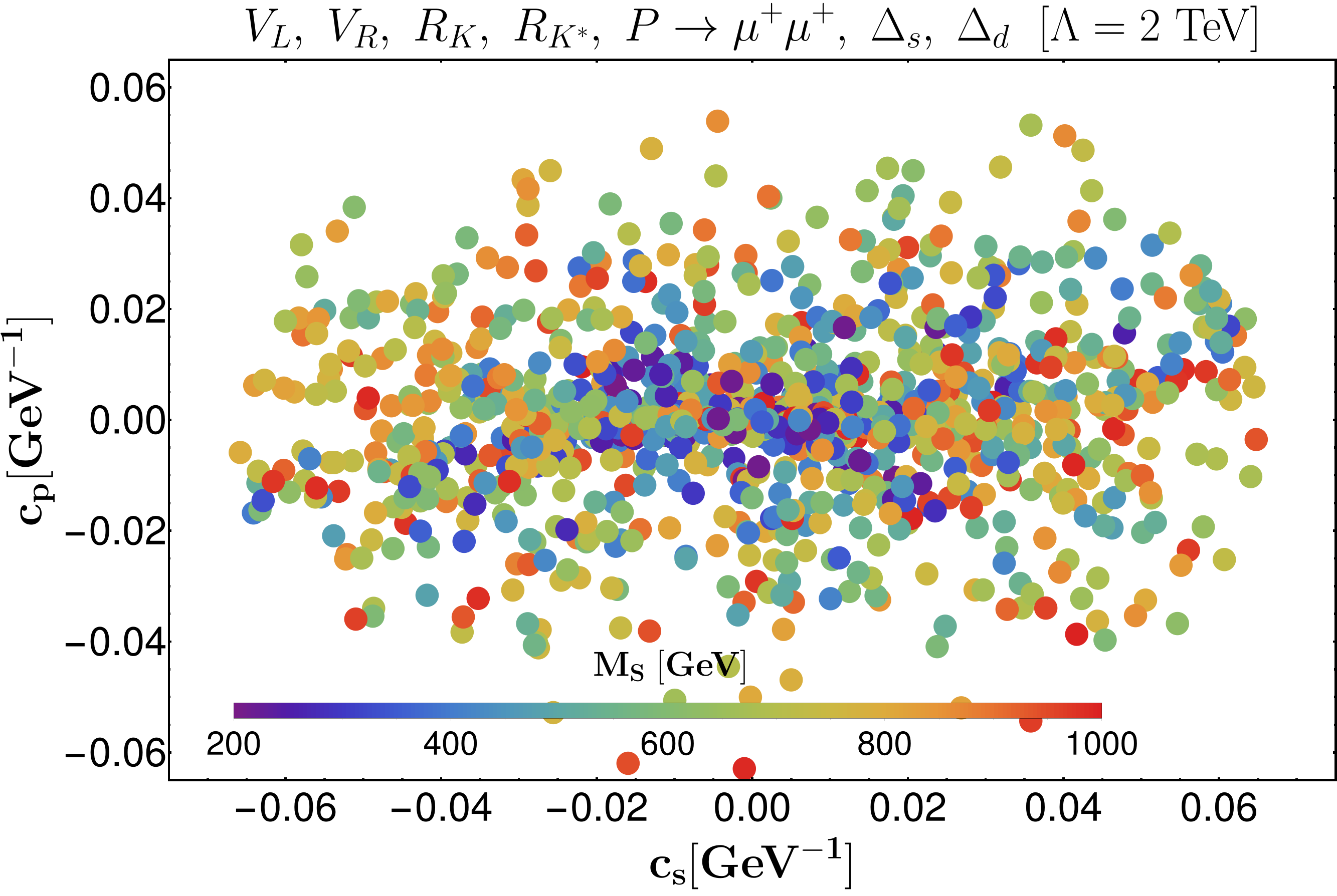
(a)

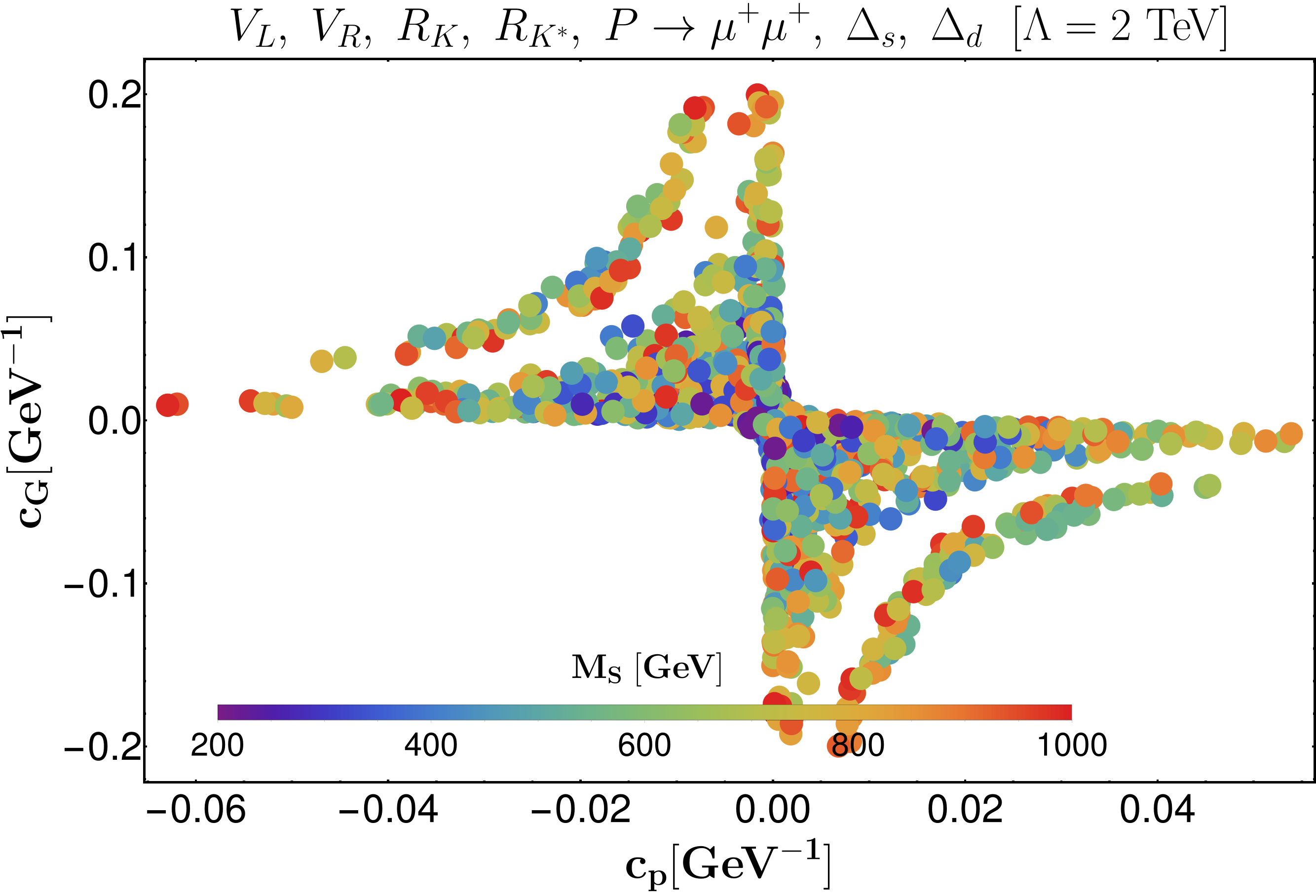
(b)

Figure 11: Allowed parameter space in $c_{s}-c_{p}$ (left) and $c_{p}-c_{G}$(right) planes obtained from a scan of the observables mentioned on the top of the figures. Also, the scalar mass $M_{S}$ has been varied (shown in colour bars).

In another analysis, we have done a parameter scan. In that analysis, we have included the data on the purely leptonic rare decays, like $\mathcal{B}(B_{s}\to\mu^{+}\mu^{-})$, $\mathcal{B}(B_{d}\to\mu^{+}\mu^{-})$, $\mathcal{B}(K_{L/S}\to\mu^{+}\mu^{-})$ and the $B_{s/d}-\bar{B}_{s/d}$ mixing amplitudes. The corresponding measured values or the upper limits we have shown in the respective paragraphs in subsection 3.1. Also, we have included the available inputs on $V_{L}$ and $V_{R}$ obtained from the study of $t\to bW$ decays, which we have shown in table 1, respectively. Note that on $V_{L}$, we have the measured value with a statistical error, while for $V_{R}$, we only have allowed ranges obtained from different other measurements. In addition, we have included the measured values of $R(K^{(*)})$. The results of the scan are shown in fig. 11. We have shown the correlations between scalar, pseudoscalar, and gauge couplings. We present the results for $\Lambda=2$ TeV. We have obtained similar parameter spaces for $\Lambda=1$ TeV, which we have not shown separately.

The allowed parameters are consistent with "zero", which is as per expectations since the data used in this analysis are consistent with the respective SM predictions. The allowed ranges are $|c_{s}|\leq 0.06$ $\text{GeV}^{-1}$, $|c_{p}|\leq 0.05$ $\text{GeV}^{-1}$ and $|c_{G}|\leq 0.2$ $\text{GeV}^{-1}$, respectively. The data allows a negative correlation between $c_{G}$ and $c_{p}$. The maximum value of $c_{p}$ could be obtained only when $c_{G}\to 0$ and vice-versa. However, we have not seen any noticeable correlation between $c_{s}$ and $c_{G}$. Also, note that the constraints are slightly tighter for $M_{S}\lesssim 500$ GeV as compared to what we have mentioned above. It is important to mention that among the rare leptonic decays, the $\mathcal{B}(B_{s/d}\to\mu^{+}\mu^{-})$ constraints the data more strongly as compared to $\mathcal{B}(K_{L/S}\to\mu^{+}\mu^{-})$. This data set will be important for the later part of the analysis. We will include these inputs in a bigger data set.

Observable	Value	Observable	Value
$|V_{ud}|$ (nucl)	$0.97373\pm 0.00009\pm 0.00053$ Xayavong:2021pkp	$|\varepsilon_{K}|$	$(2.228\pm 0.011)\times 10^{-3}$ PDG:2022
$|V_{us}|f_{+}^{K\to\pi}(0)$	$0.2165\pm 0.0004$ ParticleDataGroup:2022pth	sin $2\beta$	$0.699\pm 0.017$ HFLAV:2022
$|V_{cd}|_{\nu N}$	$0.230\pm 0.011$ PDG:2022	$\phi_{s}$	$-0.057\pm 0.021$ CKMFitter:2021
$|V_{cs}|_{W\to c\bar{s}}$	$0.94^{+0.32}_{-0.26}\pm 0.13$ ParticleDataGroup:2022pth	$\alpha$	$(85.2^{+4.8}_{-4.3})^{\circ}$ HFLAV:2022
$|V_{ub}|_{excl}$	$(3.91\pm 0.13)\times 10^{-3}$ Biswas:2022yvh	$\gamma$	$(66.2^{+3.4}_{3.6})^{\circ}$ HFLAV:2022
$|V_{cb}|_{B\to D}$	$(40.84\pm 1.15)\times 10^{-3}$ Jaiswal:2017rve	$V_{L}$	$0.995\pm 0.021$ PDG:2022
$\frac{\mathcal{B}(\Lambda_{p}\to p\mu^{-}\bar{\nu}_{\mu})_{q^{2}>15}}{\mathcal{B}(\Lambda_{p}\to\Lambda_{c}\mu^{-}\bar{\nu}_{\mu})_{q^{2}>7}}$	$(0.947\pm 0.081)\times 10^{-2}$ LHCb:2015eia	$\Delta_{s}$	$-0.0345\pm 0.0498$ DiLuzio:2019jyq ; LHCb:2021moh
$\mathcal{B}(B^{-}\to\tau^{-}\bar{\nu}_{\tau})$	$(1.09\pm 0.24)\times 10^{-4}$ HFLAV:2019	$\Delta_{d}$	$-0.0497\pm 0.0518$ DiLuzio:2019jyq ; HFLAV:2022
$\mathcal{B}(D_{s}^{-}\to\mu^{-}\bar{\nu}_{\mu})$	$(5.51\pm 0.16)\times 10^{-3}$ HFLAV:2019	$R_{b}$	$0.21629\pm 0.00066$ PDG:2022
$\mathcal{B}(D_{s}^{-}\to\tau^{-}\bar{\nu}_{\tau})$	$(5.52\pm 0.24)\times 10^{-2}$ HFLAV:2019	$R_{c}$	$0.1721\pm 0.0030$ PDG:2022
$\mathcal{B}(D^{-}\to\mu^{-}\bar{\nu}_{\mu})$	$(3.77\pm 0.18)\times 10^{-4}$ HFLAV:2019	$R_{e}$	$20.804\pm 0.050$ PDG:2022
$\mathcal{B}(D^{-}\to\tau^{-}\bar{\nu}_{\tau})$	$(1.20\pm 0.27)\times 10^{-3}$ HFLAV:2019	$R_{\mu}$	$20.784\pm 0.034$ PDG:2022
$\mathcal{B}(K^{-}\to e^{-}\bar{\nu}_{e})$	$(1.582\pm 0.007)\times 10^{-5}$ PDG:2022	$R_{\tau}$	$20.764\pm 0.045$ PDG:2022
$\mathcal{B}(K^{-}\to\mu^{-}\bar{\nu}_{\mu})$	$0.6356\pm 0.0011$ PDG:2022	$A_{e}$	$0.1515\pm 0.0019$ PDG:2022
$\mathcal{B}(\tau^{-}\to K^{-}\bar{\nu}_{\tau})$	$(0.6986\pm 0.0085)\times 10^{-2}$ HFLAV:2019	$A_{\mu}$	$0.142\pm 0.015$ PDG:2022
$\frac{\mathcal{B}(K^{-}\to\mu^{-}\bar{\nu}_{\mu})}{\mathcal{B}(\pi^{-}\to\mu^{-}\bar{\nu}_{\mu})}$	$1.3367\pm 0.0029$ PDG:2022	$A_{\tau}$	$0.143\pm 0.004$ PDG:2022
$\frac{\mathcal{B}(\tau^{-}\to K^{-}\bar{\nu}_{\tau})}{\mathcal{B}(\tau^{-}\to\pi^{-}\bar{\nu}_{\tau})}$	$(6.467\pm 0.84)\times 10^{-2}$ HFLAV:2019	$A_{s}$	$0.90\pm 0.09$ PDG:2022
$\mathcal{B}(B_{s}\to\mu^{+}\mu^{-})$	$(3.09^{+0.46~{}~{}+0.15}_{-0.43~{}~{}-0.11})\times 10^{-9}$ LHCb:2021vsc	$A_{c}$	$0.670\pm 0.027$ PDG:2022
$\mathcal{B}(B_{0}\to\mu^{+}\mu^{-})$	$(0.12^{+0.08}_{-0.07}\pm 0.01)\times 10^{-9}$ LHCb:2021vsc	$A_{b}$	$0.923\pm 0.020$ PDG:2022
$|V_{cd}|f_{+}^{D\to\pi}(0)$	$0.1426\pm 0.0018$ HFLAV:2022
$|V_{cs}|f_{+}^{D\to K}(0)$	$0.7180\pm 0.0033$ HFLAV:2022

Table 4: List of observables from FCNC, FCCC, and the Z-pole observables used in the global fit.

4.1 Fit to all the relevant FCCC, FCNC, W- and Z-pole observables

In this subsection, we will present the result of the fits to all the relevant data related to FCNC and FCNC processes discussed in subsection 3.1 and 3.2, respectively. Also, we have included the W-pole and the $Z$-pole observables. The details of various inputs used in the fit are presented in tables 4 and 2, respectively. The other relevant theory inputs can be seen in table 8 in the appendix. In addition, we have included the data on $R(K^{(*)})$ given in eq. (37a) and we have not included the data on the differential rates and the angular observables of $B\to K^{(*)}\mu^{+}\mu^{-}$ and $B_{s}\to\phi\mu^{+}\mu^{-}$ decays which have negligible impact on our conclusions.

We have analysed the data for the cases $c_{s}\neq c_{p}$, $c_{s}=c_{p}$, and $c_{s}=0$, respectively, and presented the fit results for a few fixed values of $M_{S}$. Alongside the fits, we have scanned the parameter spaces using all the available data mentioned above. The results of the scan will be helpful to understand the correlations among the NP parameters. Also, we will be able to understand the dependence of the fit results on the scalar mass $M_{S}$.

$\Lambda$ $\rm[TeV]$	$M_{S}$ $\rm[GeV]$	$c_{s}\times 10^{2}$ $\rm[GeV^{-1}]$	$c_{p}$ $\rm[GeV^{-1}]$	$c_{G}\times 10^{3}$ $\rm[GeV^{-1}]$	$\Delta M_{W}\times 10^{2}$ $\rm[GeV]$
	$250$	$-0.090\pm 1.747$	$0.0\pm 0.018$	$2.770\pm 0.259$	$4.657\pm 0.869$
	$500$	$0.162\pm 2.014$	$0.0\pm 0.020$	$3.432\pm 0.321$	$4.654\pm 0.869$
$1$	$800$	$0.566\pm 3.616$	$0.0\pm 0.033$	$4.487\pm 0.419$	$4.645\pm 0.869$
	$250$	$-0.130\pm 1.493$	$0.0\pm 0.015$	$2.305\pm 0.215$	$4.658\pm 0.869$
	$500$	$-0.018\pm 1.560$	$0.0\pm 0.015$	$2.646\pm 0.247$	$4.656\pm 0.869$
	$800$	$0.107\pm 1.693$	$0.0\pm 0.016$	$3.048\pm 0.285$	$4.653\pm 0.869$
$2$	$1000$	$0.197\pm 1.829$	$0.0\pm 0.017$	$3.330\pm 0.311$	$4.651\pm 0.869$

Table 5: Fit results of the parameters $c_{s},~{}c_{p}$ and $c_{G}$ for different combinations of $\Lambda$ and $M_{S},$ all the observables of table 4 along with $\delta(\Delta r)$ (CDF, LHCb, ATLAS, D0) are taken into account, with a p-value of $\sim 3\%$ for 45 d.o.f. The last column shows the prediction of the value of $\Delta M_{W}$ from this fit result for each case.

$\Lambda$ [TeV]	$M_{S}$ $\rm[GeV]$	$c_{s}\times 10^{2}$ $\rm[GeV^{-1}]$	$c_{p}$ $\rm[GeV^{-1}]$	$c_{G}\times 10^{3}$ $\rm[GeV^{-1}]$	$\Delta M_{W}\times 10^{2}$ $\rm[GeV]$
	$250$	$0.027\pm 1.734$	$0.0\pm 0.018$	$-0.820\pm 1.413$	$0.409\pm 1.408$
	$500$	$-0.048\pm 1.953$	$0.0\pm 0.020$	$-1.013\pm 1.755$	$0.406\pm 1.405$
$1$	$800$	$-0.172\pm 2.239$	$0.0\pm 0.022$	$-1.333\pm 2.275$	$0.410\pm 1.399$
	$250$	$0.038\pm 1.457$	$0.0\pm 0.015$	$-0.684\pm 1.174$	$0.410\pm 1.409$
	$500$	$0.005\pm 1.558$	$0.0\pm 0.016$	$-0.782\pm 1.353$	$0.407\pm 1.408$
	$800$	$0.032\pm 1.662$	$0.0\pm 0.017$	$0.899\pm 1.546$	$0.405\pm 1.392$
$2$	$1000$	$0.058\pm 1.726$	$0.0\pm 0.017$	$0.982\pm 1.690$	$0.404\pm 1.391$

Table 6: Fit results of the parameters $c_{s},~{}c_{p}$ and $c_{G}$ for different combinations of $\Lambda$ and $M_{S},$ when all the observables of table 4 are considered along with weighted mean data of $\delta(\Delta r)$ observable from LHCb, ATLAS and D0 experiment LHCb:2021bjt ; ATLAS:2017rzl ; ATLAS:2023fsi ; D0:2012kms . The p-value for the fit is $\sim 30.49\%$ with 42 d.o.f. The last column shows the prediction of the $\Delta M_{W}$ value from this fit result for each case.

	Predictions: SM and NP (for $\Lambda=2$ TeV)
Obs.	SM	$M_{S}=500$ GeV	$M_{S}=1000$ GeV
$R_{b}$	0.215820(20)	0.215814(20)	0.215812(20)
$R_{c}$	0.172210(30)	0.172199(30)	0.172195(30)
$R_{e}$	20.7360(100)	20.7306(100)	20.7286(101)
$R_{\mu}$	20.7360(100)	20.7310(100)	20.7290(100)
$R_{\tau}$	20.7810(100)	20.7743(100)	20.7724(100)
$A_{e}$	0.146800(300)	0.146830(300)	0.146840(300)
$A_{\mu}$	0.146800(300)	0.146830(300)	0.146840(300)
$A_{\tau}$	0.146800(300)	0.146830(300)	0.146840(300)
$A_{s}$	0.934700(0)	0.934741(8)	0.934755(10)
$A_{c}$	0.667700(100)	0.667802(102)	0.667836(103)
$A_{b}$	0.935600(0)	0.935668(13)	0.935690(17)

Table 7: Prediction of the Z-pole ratio and asymmetric observables for the case $c_{s}\neq c_{p}\neq 0.$ Here, the prediction is shown for $\Lambda=2\rm TeV.$

We have presented our results based on whether or not we have included in the fit the estimate of $\delta(\Delta r)$ by the CDF (table 2). In table 5, we have presented the result of a fit, which includes all the data we have mentioned above. The p-value of the fit is $\approx$ 3%, which is a statistically allowed fit. The results are obtained for $\Lambda=1$ and 2 TeV, respectively, for a few values of $M_{S}$. Note that for $\Lambda=2$ TeV, for $M_{S}\approx 1000$ GeV for both the $c_{p}$ and $c_{s}$, the maximum allowed values are $<0.02$ GeV^-1. On the other hand, for $\Lambda=1$ TeV, the allowed values could be as large as $\approx 0.03$ GeV^-1 for higher values of $M_{S}$. For lower values of $M_{S}$, the maximum allowed values will be reduced. On the other hand, the gauge coefficient $c_{G}$ has non-zero allowed values, though very small. The $W$- and $Z$-pole observables are highly sensitive to $c_{G}$. The non-zero values of $c_{G}$ are allowed due to the data on $M_{W}$ by CDF, which deviates from the SM. Note that with the increasing value of $M_{S}$, the bounds on $c_{G}$ are a little relaxed, as compared to those bounds obtained for lower values of $M_{S}$. For the values of $M_{S}$ we have considered in this analysis, the allowed value of $c_{G}$ is of order $\mathcal{O}(10^{(-3)})$. In table 6, we have presented the results of a fit in which we have not taken the input on $\delta(\Delta r)$ from CDF. We note an increase in the quality of the fit, which is indicated by an increase in the $p$ value of the fits. The constraints on $c_{p}$ and $c_{p}$ do not change much, and we have similar observations. However, the allowed values of $c_{G}$ now become zero consistent, and the maximum allowed values are of order $\mathcal{O}(10^{-3})$. The explicit numbers can be seen from the table.

Using the results of the fits, we have predicted the respective values of $\Delta M_{W}$, which is a shift of the value of $M_{W}$ from the corresponding SM predictions. For the fit results, which include the data on $M_{W}$ from CDF, we note a slight non-zero shift $\Delta M_{W}\approx 0.05$ GeV. However, from the results of the fits without the CDF input, we have not observed a non-zero shift in $\Delta M_{W}$, it is fully consistent with the SM. In addition, we have predicted all the Z-pole observables, shown in table 7 using the results of the fit given in table 6. We note that the predicted values of all the Z-pole observables are fully consistent with the respective data and the SM predictions. This indicates that in our simplified model, it is possible to explain the observed deviation in $M_{W}$ by CDF and the measured precise values of the Z-pole observables.

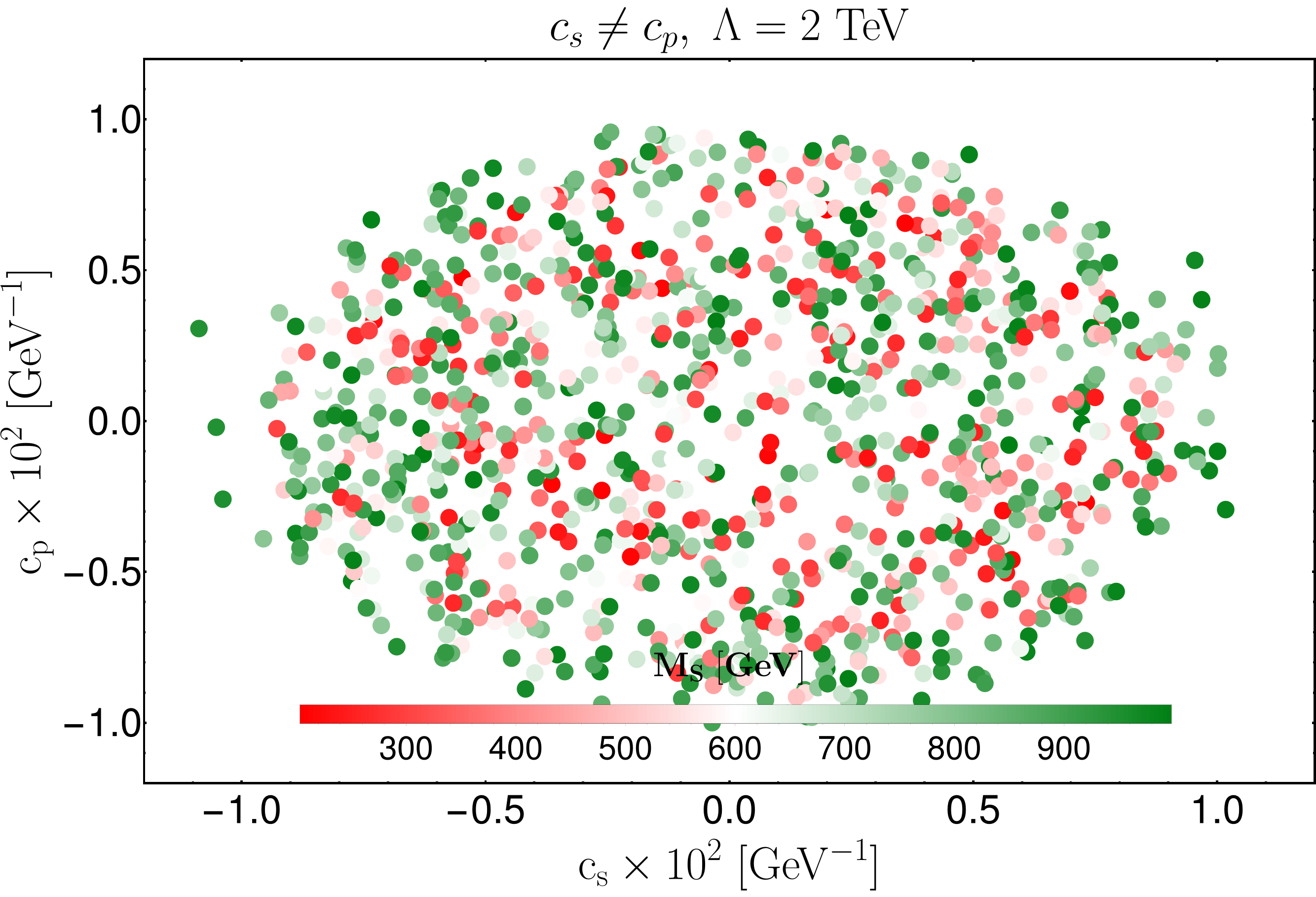
(a)

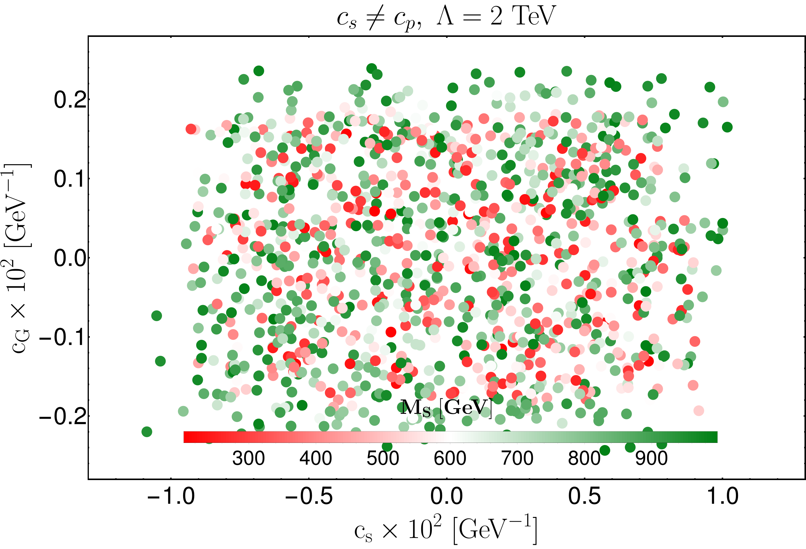
(b)

Figure 12: The allowed parameter space in the $c_{s}$-$c_{p}$ and $c_{p}$-$c_{G}$ planes for $\Lambda=2~{}\rm TeV$ is determined by considering all flavour and electroweak observables.

As we have mentioned earlier, to get an idea about the relevant correlations between the couplings, we have done the scan using the data given in tables 4, 2 and eq. (37a), respectively. The results of the scan are given in fig. 12. In these scans, we have dropped the input on the $\delta(\Delta r)$ from CDF. Within the allowed regions of $c_{p}$, $c_{s}$, and $c_{G}$, we do not see any strong correlation between these three couplings. Also, the allowed ranges are consistent with the fit results given in table 10. We notice a slight increase in the allowed regions of the couplings for higher values of $M_{S}$. In addition, the correlation between $c_{s}$ and $c_{p}$ indicates that for $c_{s}=0$, the allowed range of $c_{p}$ will not change. Hence, the analysis with $c_{s}=0$ will give us the same allowed/fitted values of $c_{p}$ as we have obtained in tables 9 and 10, respectively. We have not presented those results separately.

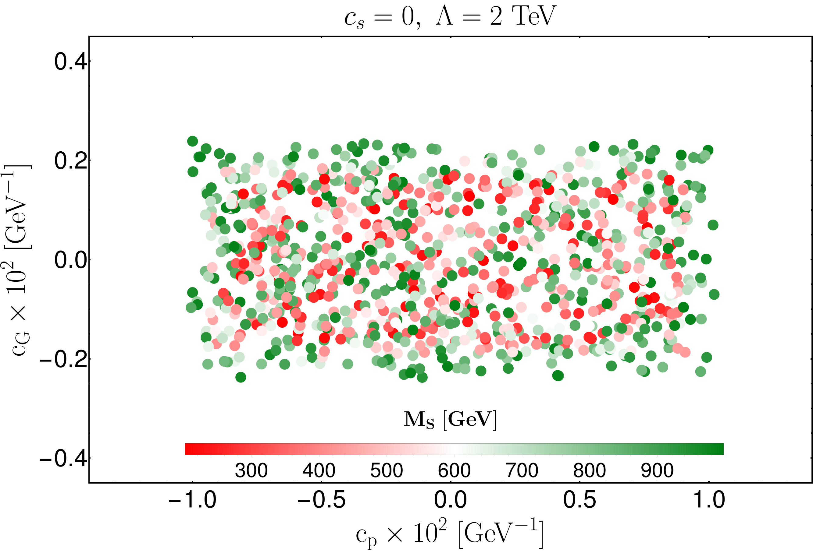
(a)

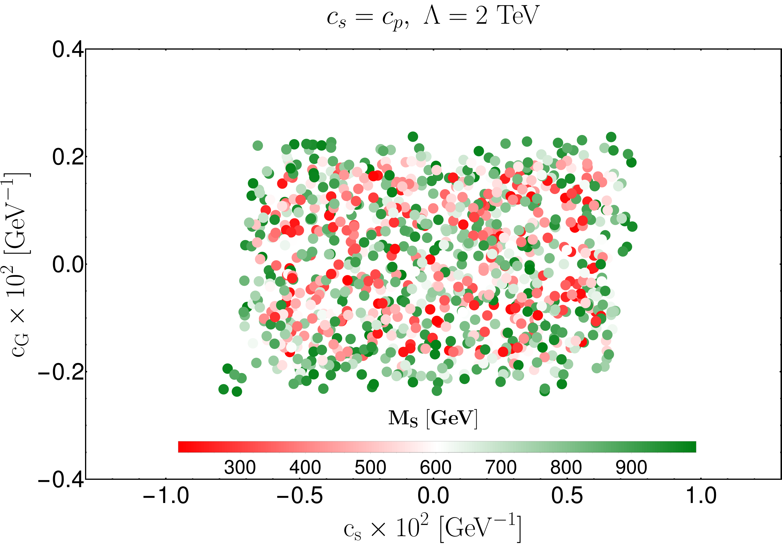
(b)

Figure 13: Allowed parameter space in $c_{p}-c_{G}$ plane, when we have set $c_{s}=0$ (left) and $c_{s}=c_{p}$ (right). To generate these plots, we have varied $M_{S}$ over a range of 200 to 1000 GeV.

We have separately presented the results of the analyses of the scenario $\bf c_{s}=c_{p}$ in tables 9 and 10, respectively, with and without the inputs on $\delta(\Delta r)$ from CDF. The other inputs are similar to the one discussed above. The constraints on $c_{p}(=c_{s})$ and $c_{G}$ remain same as before. Also, in such a case, we will be able to explain $\Delta M_{W}$ and all the Z-pole observables simultaneously. In fig. 13, we have shown the correlations between $c_{p}$ and $c_{G}$ in the scenarios $c_{s}=0$ (left plot) and $c_{p}=c_{s}$ (right plot). Like before, we do not see any noticeable correlations between these coefficients, and the allowed regions are similar to those obtained from the fits.

5 Phenomenology of Dark Matter and Flavour

(a)

(b)

(c)

(d)

Figure 14: Feynman diagrams depicting the annihilation channels of the DM are significant for determining relic density.

(a)

(b)

Figure 15: Feynman diagrams contribute to the direct detection process (left) and to the indirect detection for annihilation to $b\bar{b}$ (right).

In our simplified model, we consider a fermionic DM with a spin-0 mediator given in eqs. (1) and (2.1.1), respectively. As we know, the WIMP-type dark matter gives the current relic density by the freeze-out method. The relevant diagrams for Dark matter pair annihilation to the SM particles are given in fig 14, respectively. The mediator $S$ interacts with SM fermions and gauge bosons. Hence, the dominant channel for DM annihilation will be $\bar{\chi}\chi\rightarrow\bar{f}f$ and $\bar{\chi}\chi\rightarrow VV$ (V for $W_{\mu},Z_{\mu}$). DM can also annihilate to gluon via a penguin loop shown in fig 14d. For $m_{\chi}\leq M_{S}$, DM will mostly annihilate to these channels. For the case, $m_{\chi}\geq M_{S}$, a significant contribution will come from the t-channel annihilation diagram of DM, i.e., $\chi\bar{\chi}\to SS.$ At resonance, contribution from s-channel annihilation diagrams will be more. We have specified earlier that in order to maintain MFV, we use the mass-dependent coupling of the spin-0 mediator with SM fermions (similar to the SM-Yukawa). So, the coupling with the top quark is maximum. Using that fact, we will get another channel contributing to our case $\chi\bar{\chi}\to gg.$ The effective coupling is given by Buckley:2014fba :

$$\mathcal{L}_{gluon}=\frac{\alpha_{s}}{8\pi}\biggl{(}c_{s}\tau[1+(1-\tau)f(\tau)]G^{\mu\nu}G_{\mu\nu}+2c_{p}\tau f(\tau)G^{\mu\nu}\tilde{G}_{\mu\nu}\biggr{)}S\,,$$ (92)

Where, $\tau=\frac{4m_{t}^{2}}{M_{S}^{2}}$ and

$$f(\tau)=\begin{cases}\arcsin^{2}\frac{1}{\sqrt{\tau}}&\text{if }~{}\tau\geq 1\\ -\frac{1}{4}(\log\frac{1+\sqrt{1-\tau}}{1-\sqrt{1-\tau}}-i\pi)^{2}\,&\text{if }~{}\tau<1\end{cases}$$

This type of contribution will play an important role when $M_{\chi}<m_{t}$. In our case, most contributions will come from $t\bar{t}\text{ and }~{}VV$ processes; we still consider it.

As expected, in our model, we will also get a non-zero contribution to the scattering cross-section of the DM with the nucleon, which is relevant for the direct detection process, where we study the recoil energy of the detector nuclei. The upper bounds of such processes are obtained in various measurements, among which the most stringent bound comes from XenonnT XENON:2023cxc , LUX-ZEPLIN LZ:2022lsv and Panda4X-TPandaX:2023ejt . In this work, we have used the bound from XenonnT and LUX-ZEPLIN, which are more stringent than PandaX-4T. Also, the study of gamma-ray annihilation spectrum in indirect detection gives bound on DM annihilation cross-section rate to SM particle pairs ($b\bar{b},~{}W^{+}W^{-},~{}\tau^{+}\tau^{-}$ etc) the collaborations like Fermi-LAT Fermi-LAT:2015att ; Fermi-LAT:2016afa , High Energy Stereoscopic System (H.E.S.S) HESS:2016mib and Cherenkov Telescope Array (CTA) Silverwood:2014yza provide bounds on that.

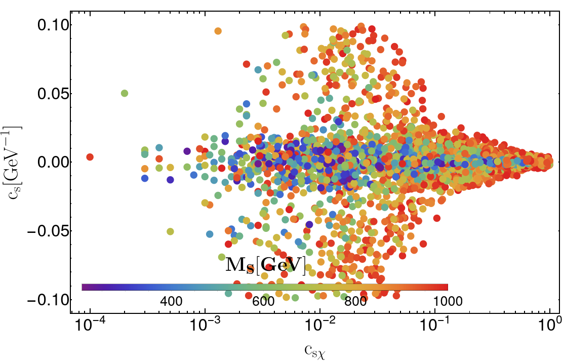
(a)

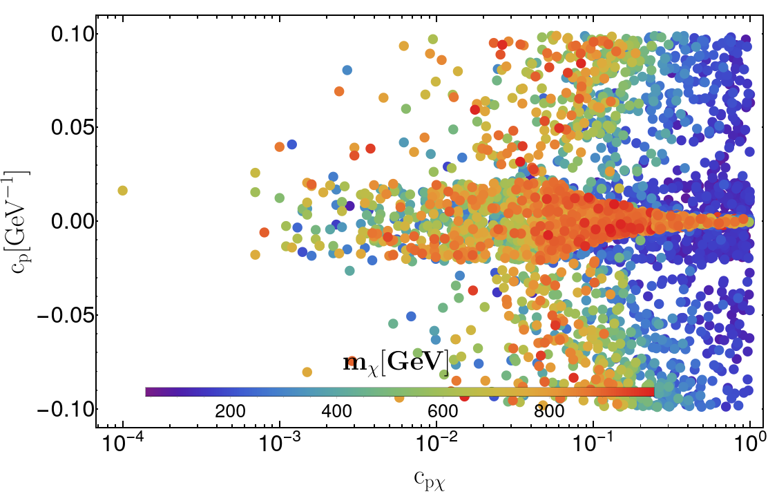
(b)

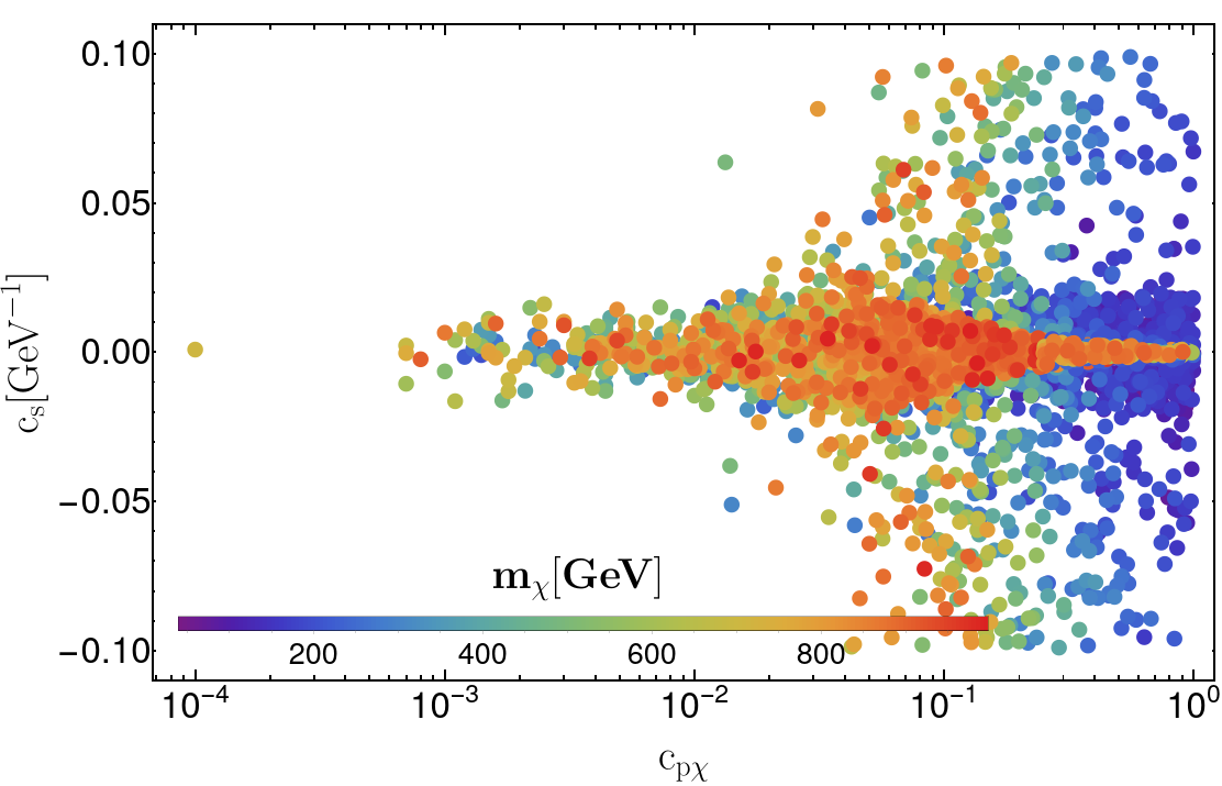
(c)

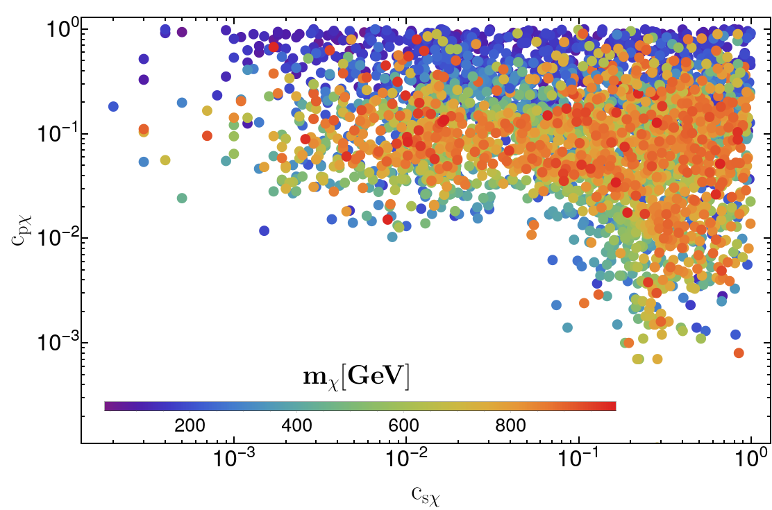
(d)

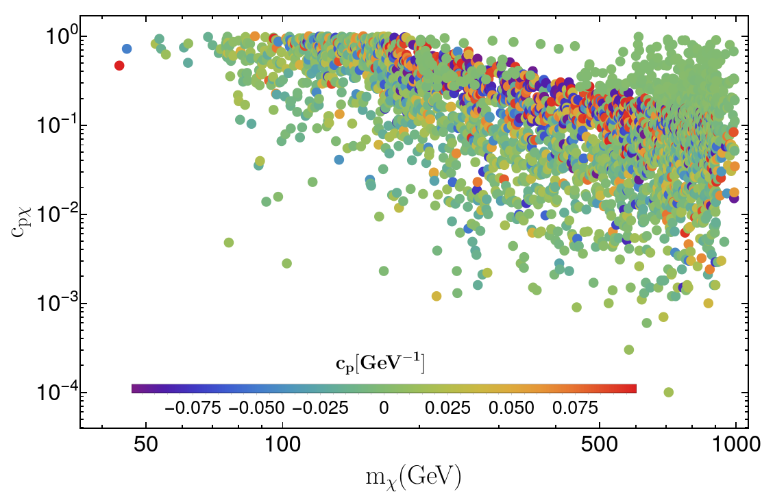
(e)

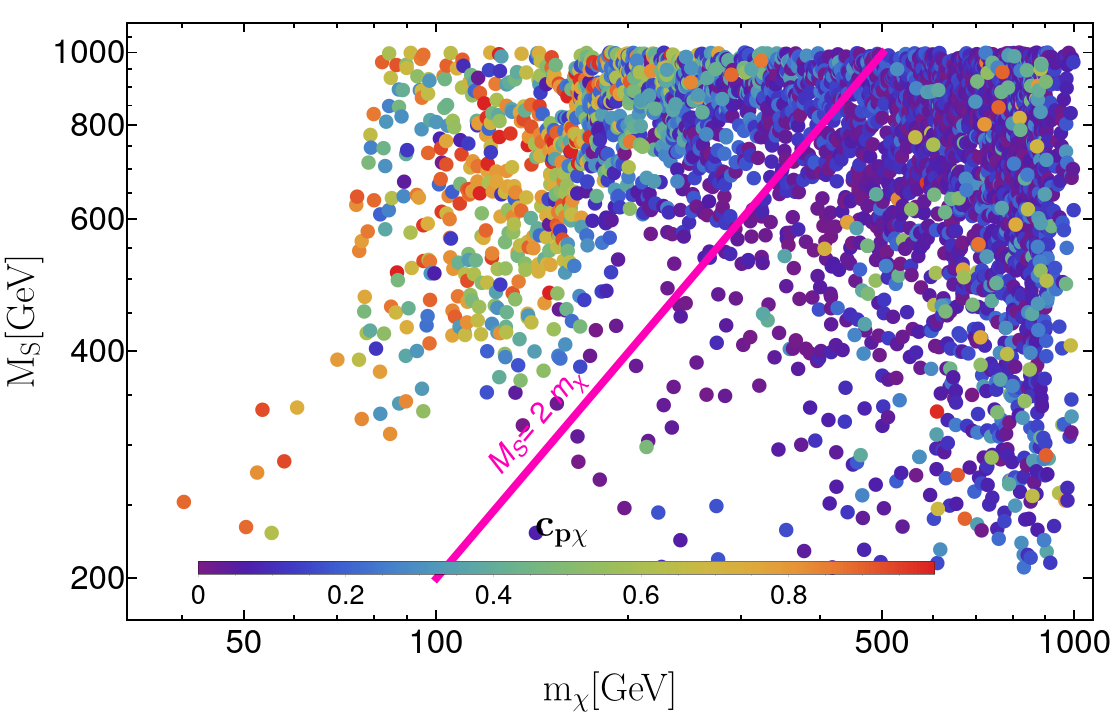
(f)

Figure 16: Correlation among the couplings $c_{s},~{}c_{p},~{}c_{s\chi},~{}c_{p\chi}$ and $~{}c_{G}$ All the points in the plots are allowed by observed relic density data and direct detection cross-section bound provided by LUZ-ZEPLIN 2022.

5.1 Results of the analysis

We have analysed the data on relic density and the direct detection cross-section separately and in combination with the flavour data and obtained the constraints on the new physics parameters. At first, we have treated the scalar mass $M_{S}$, the DM mass $m_{\chi}$ and all the relevant couplings, like $c_{s\chi}$, $c_{p\chi}$, $c_{s}$, $c_{p}$ and $c_{G}$ as free parameters and obtained the bounds from the data on relic density and direct detection cross-section. The results of the scan are presented as correlations between different variables in fig. 16. We have varied both the couplings $c_{s\chi}$ and $c_{p\chi}$ of DM to the scalar $S$ over the range $[-1.0,1.0]$, and the masses $M_{S}$ and $m_{\chi}$ over the range 100 GeV to 1000 GeV. To understand these correlations, we must note that the scalar current contribution to the $s$-channel annihilation cross-section is the velocity-suppressed p-wave contribution (for details, please see appendix E). However, the pseudoscalar current contribution to the s-channel cross-section will be the s-wave contribution, which is not velocity-suppressed. In our analysis, the s-wave annihilation cross section will be $\propto c^{2}_{p\chi}(c_{s}^{2}+c_{p}^{2})$ and velocity suppressed p-wave contribution is $\propto c^{2}_{s\chi}(c_{s}^{2}+c_{p}^{2})$. Also, these cross-sections are proportional to the square of the dark matter mass and inversely proportional to $(M^{2}_{S}-4m^{2}_{\chi})^{2}$. On the other hand, in our simplified model, the dominating contribution to spin-independent direct detection cross section is proportional to $c^{2}_{s\chi}c^{2}_{s}$, the rest of the contributions are velocity suppressed. Hence, we will get a tight bound on this product from the direct detection bound. Below, in the items, we will make a few remarks on the correlations between parameters from fig. 16.

• In fig. 16a, we have shown the correlation between $c_{s\chi}$, $c_{s}$ and $M_{S}$ (in colour band). As mentioned in the above paragraph, the strong bound on the product $c^{2}_{s\chi}c^{2}_{s}$ will come from the spin-independent direct detection cross-section. We note that for values $c_{s\chi}>0.1$, the allowed values of $c_{s}$ will be highly constrained and small, also in this region, $M_{S}\gtrsim 600$ GeV. This is because the direct detection cross-section decreases with the increase of mediator mass. Hence, for relatively higher values of $M_{S}$, the direct detection bound will allow relatively larger values of $c_{s\chi}$. In the region $c_{s\chi}<0.1$, the allowed values of $c_{s}$ are relatively relaxed, and the allowed values of $c_{s}$ will be of order $10^{-3}$ or less only when $M_{S}<500$ GeV.

• In fig. 16b we have shown the correlation between $c_{p\chi}$, $c_{p}$ and $m_{\chi}$. Note that for $m_{\chi}>500$ GeV, the allowed values of $c_{p\chi}$ will be $>0.3$ only when $c_{p}$ is of order $10^{-3}$ or less. However, for $c_{p\chi}<0.1$, the allowed values of $c_{p}$ have a wide range, and they could be as large as order one. For $m_{\chi}<500$ GeV the large values $(\mathcal{O}(1))$ of both $c_{p\chi}$ is allowed by the data on relic density. In such a situation, relatively higher values of $c_{p}$ are also allowed. A similar observation holds for the correlation between $c_{s}$ and $c_{p\chi}$, which we have shown in fig. 16c.

• In fig. 16d, we have shown the correlations between $c_{s\chi}$, $c_{p\chi}$ and $m_{\chi}$ (colour band). Note that for $c_{s\chi}\lesssim 0.1$, the allowed values of $c_{p\chi}>0.02$. Also, in such a situation, $c_{p\chi}$ could be of order one when $m_{\chi}\lesssim 350$ GeV. The allowed solutions for $m_{\chi}>400$ GeV prefers values of $c_{p\chi}\approx 0.1$. In the regions $c_{p\chi}\gtrsim 0.1$ and $c_{s\chi}\gtrsim 0.1$, depending on the values of $c_{p}$ and $c_{s}$ we have allowed solutions for $100<m_{\chi}<1000$ (in GeV), which can also be seen in fig. 16e. In addition, there exists a solution in the region $0.01\lesssim c_{p\chi}\lesssim 0.001$ for $c_{s\chi}>0.1$ and $m_{\chi}\gtrsim 400$ GeV. We can see from figs. 16b, 16c and 16e this allowed region belongs to the values of $c_{s}$ of order $10^{-3}$ and for $c_{p}\lesssim 0.03\rm~{}GeV^{-1}$. For such small values of $c_{p\chi}$, the contribution to the relic from the velocity-suppressed scalar current could be important.

• In fig. 16f we have shown the correlations between $M_{S}$, $m_{\chi}$ and $c_{p\chi}$ (colour band). Note that for lower values of the DM masses ($m_{\chi}\lesssim 300$ GeV), there are concentrations of allowed solutions near $M_{S}\gtrsim 500$ GeV and $c_{p\chi}>0.4$. Actually, this region belongs to $M_{S}>2m_{\chi}$. On the other hand, for $c_{p\chi}\lesssim 0.4$, the greater concentration of the allowed solutions will be for $M_{S}>400$ GeV and $m_{\chi}>300$ GeV. Note that in this region, the factor $(M_{S}^{2}-2m_{\chi^{2}})^{2}$ is small, and the annihilation cross-section will increase, hence to satisfy the data on a relic, the product $c_{p\chi}^{2}(c_{p}^{2}+c_{s}^{2})$ should decrease. Also, solutions exist in the region $m_{\chi}>M_{S}$ but with a low concentration of allowed points.

It is to be noted that for the range of the mediator mass $M_{s}\geq 100~{}GeV,$ the dominating annihilation channels will be $\chi\bar{\chi}\to f\bar{f},VV$, where $V$ stands for vector boson. More precisely, for $m_{\chi}\geq m_{t}$, $\chi\bar{\chi}\to t\bar{t}$, will contribute most to the relic density. For $m_{\chi}\leq m_{t},$ channels like $\chi\bar{\chi}\to b\bar{b},~{}W^{+}W^{-},~{}ZZ$ will have maximum contribution. Also, for $m_{\chi}\geq M_{S},$ t-channel annihilation will play a significant role. The corresponding solutions can be seen in fig. 16f.

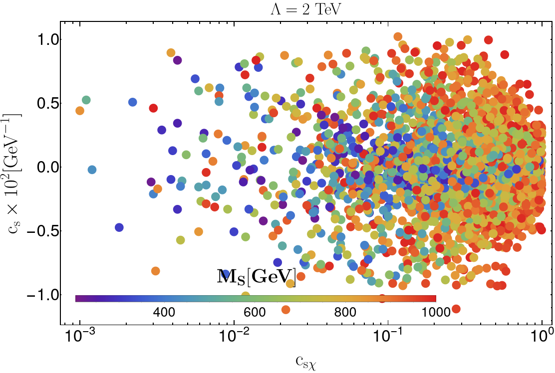
(a)

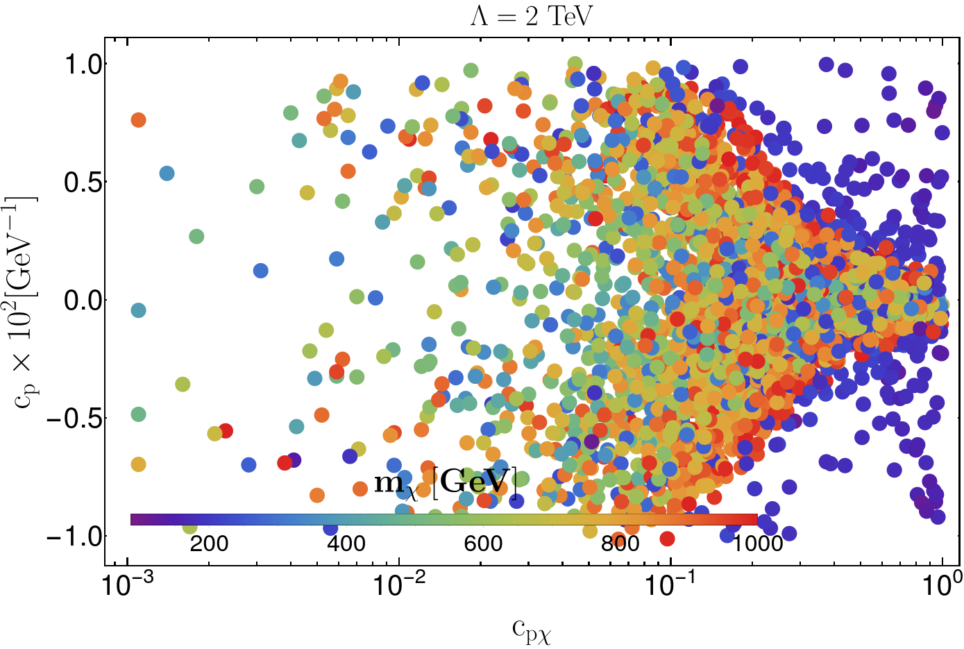
(b)

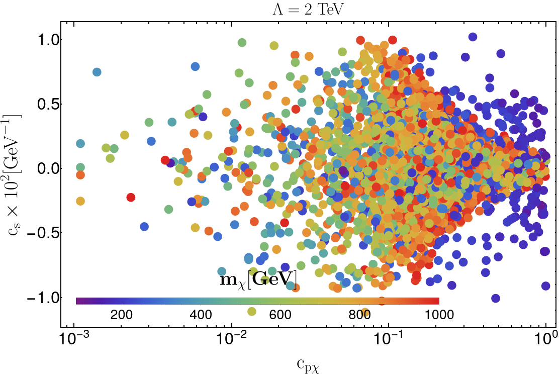
(c)

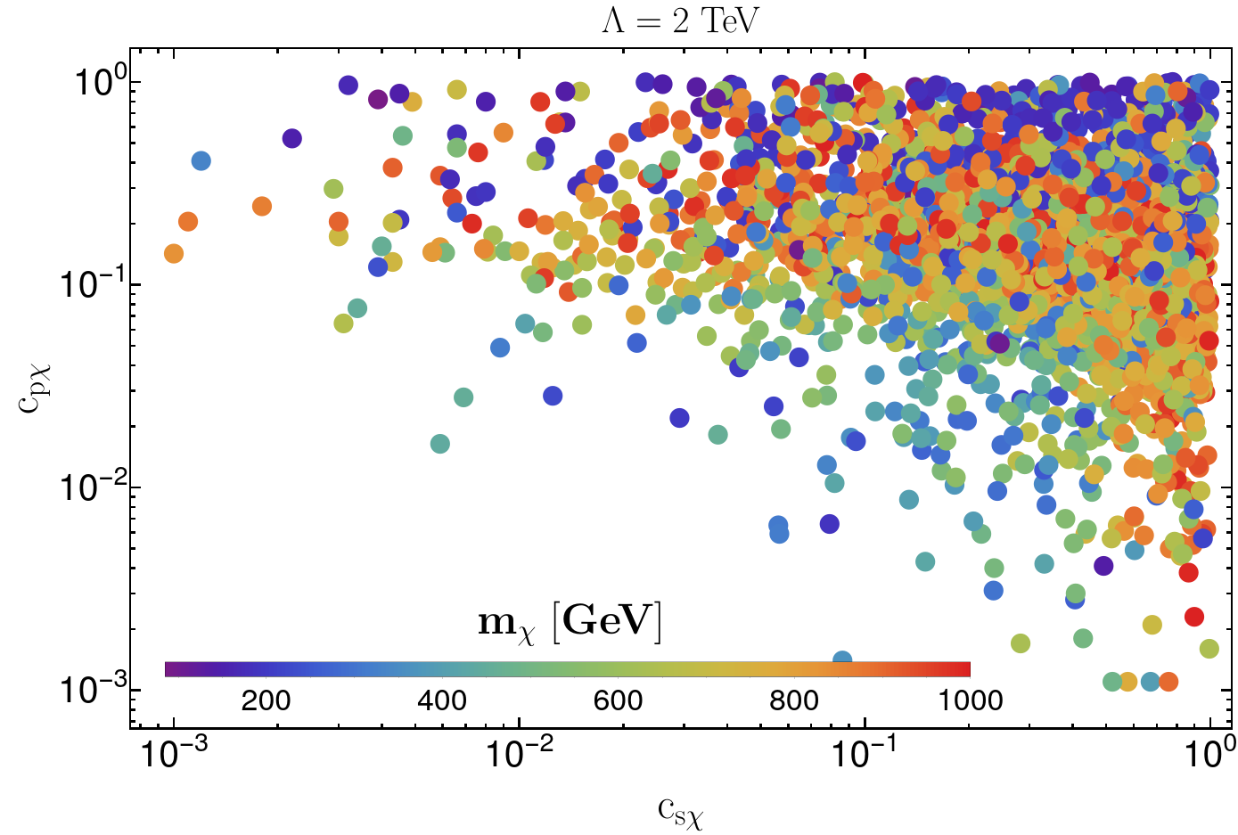
(d)

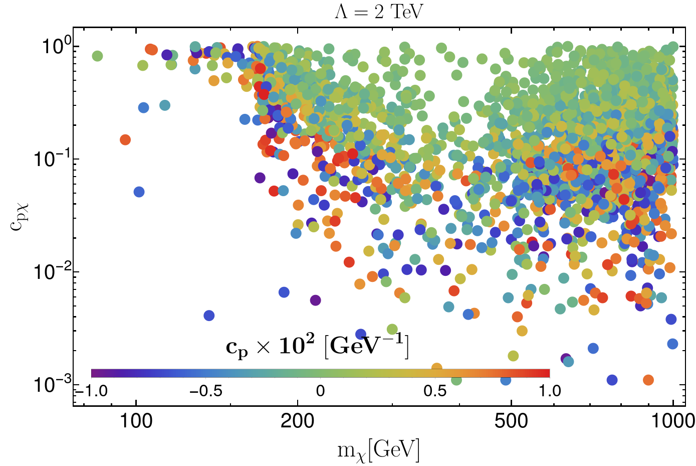
(e)

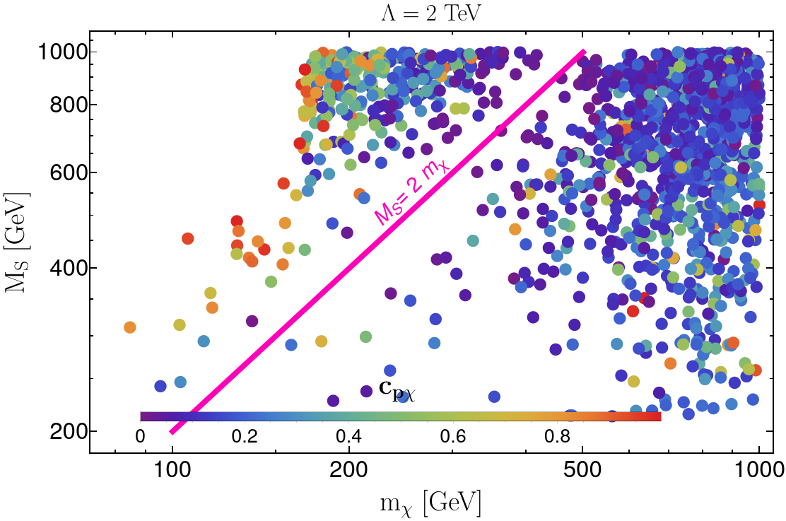
(f)

Figure 17: Correlation among the couplings $c_{s},~{}c_{p},~{}c_{s\chi},~{}c_{p\chi}$ and $~{}c_{G}$ and DM and mediator mass, from a simultaneous analysis where all the observables relevant to us, taken into account including flavour changing charged and neutral current, electroweak precision observables as well as dark sector constraints.

The correlated parameter spaces satisfying the relic density and direct detection bounds are then used to scan the flavour constraints discussed earlier. In this scan, we will not get any direct bounds on the $c_{s\chi}$, $c_{p\chi}$ and $m_{\chi}$. However, these three variables are correlated with each other and with $c_{s}$, $c_{p}$ and $M_{S}$, respectively. Hence, constraints on $c_{s}$, $c_{p}$ and $M_{S}$ from the flavour data will indirectly put constraints on $c_{s\chi}$, $c_{p\chi}$ and $m_{\chi}$. From the scan, we noticed that approximately 25% of the correlated allowed points of the DM analysis survived the flavour constraints. Hence, many of the allowed solutions for the DM mass and its coupling to the mediator will be discarded. In fig. 17, we have shown the allowed parameter spaces and their correlations, which satisfy the data on the observables related to FCNC, FCCC processes, the W- and Z-pole observables, the relic density, and the direct detection cross-section. Note that to generate these parameter spaces, we do not include the CDF data on W-mass, which shows a large deviation from the rest. However, we have done a separate scan including only this data on $W$ mass, which we have shown in Fig. 18, respectively.

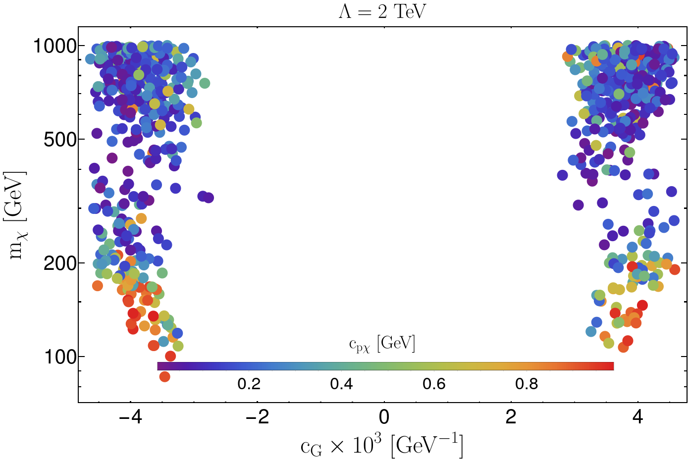
(a)

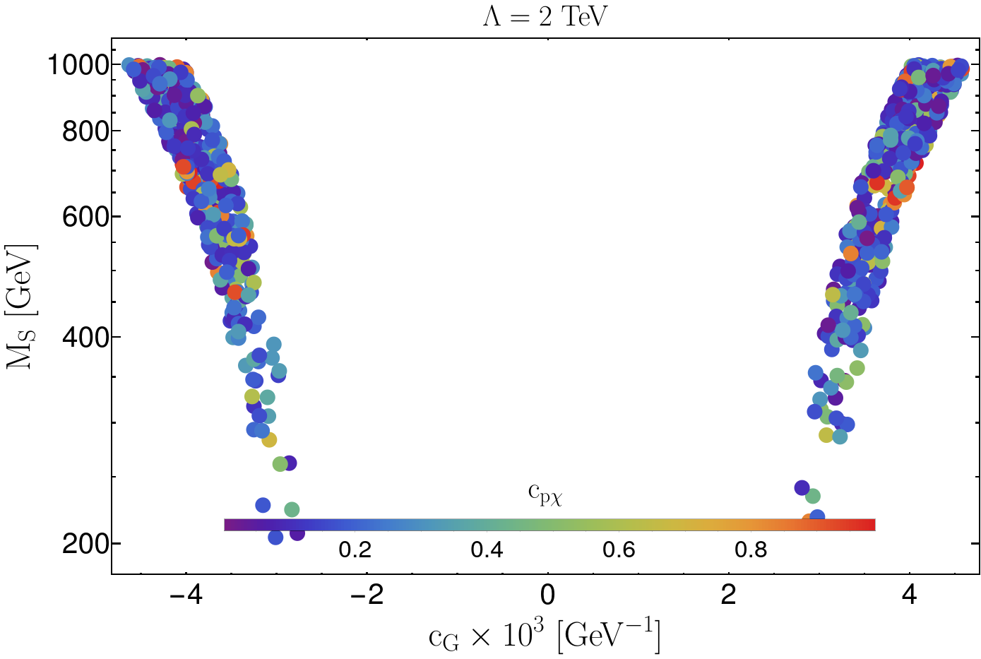
(b)

Figure 18: Correlation among the gauge coupling $c_{G}$ and DM and mediator masses, when we have taken the input of $\delta(\Delta r)$ only by CDF into account, along with all the other observables mentioned above.

As we have seen earlier, the analysis, including data other than the relic and direct detection cross-section, restricts the parameter spaces for $c_{s}$, $c_{p}$, and $c_{G}$. We have studied the correlations between these parameters, and the results are similar to those presented in plots of fig. 12. In addition, as expected, the correlations between these parameters do not depend much on the variation of the DM mass. In the analysis without the CDF data on the W-mass, the bound is consistent with the bound obtained in the analysis without the relic and the direct detection cross-section. Also, in the allowed region, $c_{G}$ does not have any noticeable correlations with the other parameters. Therefore, we will not show them separately. The allowed value of the gauge coupling $|c_{G}|$ is $\lesssim 0.002\rm~{}GeV^{-1}$.

In the items below we will summarised a few important points of the correlation plots in fig. 17.

• Like before, in fig. 17a, we have shown the correlations between $c_{s\chi}$, $c_{s}$ and $M_{S}$ (in colour band). We have more allowed solutions for $M_{S}\gtrsim 500$ GeV for $c_{s\chi}>0.01$. Also, in this region of $M_{S}$ for $0.01<c_{s\chi}\lesssim 0.2$, the maximum allowed values of $|c_{s}|$ could be near to $0.01\rm~{}GeV^{-1}$. However, for $c_{s\chi}\gtrsim 0.3$ the allowed region of $|c_{s}|$ is shrinking towards the values $<0.005\rm~{}GeV^{-1}$, and for a solution $c_{s\chi}\approx 1.0$, the allowed values will be $|c_{s}|\lesssim 0.001$. These constraints on $c_{s}$ are further stricter in the region $M_{S}<400$ GeV. In this limit, the value $|c_{s}|$ is $<0.005$ even when $0.01<c_{s\chi}\lesssim 0.1$ which will reduce further for higher values of $c_{s\chi}>0.1$.

• In figs. 17b and 17c, we have shown the correlations of $c_{p\chi}$ with $c_{p}$ and $c_{s}$ (the variation in $m_{\chi}$ is shown in colour bands), respectively. Here, also, we see the high density of the allowed solutions for $c_{p\chi}\gtrsim 0.05$ for the region of DM mass we have considered. For $c_{p\chi}\lesssim 0.1$, the allowed values of both the $|c_{s}|$ and $|c_{p}|$ will be $\lesssim 0.01\rm~{}GeV^{-1}$. However, one should note that there is a correlation between $c_{s}$ and $c_{p}$, which we have shown in fig. 12. Note that for values of $|c_{s}|$ around $0.01\rm~{}GeV^{-1}$, $|c_{p}|$ will have solutions $\lesssim 0.005\rm~{}GeV^{-1}$ and vice versa. For $M_{S}\gtrsim 500$ GeV in the region $c_{p\chi}>0.5$ the allowed regions of $c_{s}$ and $c_{p}$ are gradually shrinking with the increasing values of $c_{p\chi}$, and approaches the values $|c_{s(p)}|\lesssim 0.001\rm~{}GeV^{-1}$ when $c_{p\chi}$ approaches towards $1.0$. For $m_{\chi}<400$ GeV, $c_{p}$ or $c_{s}$ could achive a value around $0.005\rm~{}GeV^{-1}$ even though $c_{p\chi}\approx 1.0$.

• We can make a similar observation as in item-2 after a close inspection of the correlation between $c_{p\chi}$ and $m_{\chi}$ in fig. 17e. We note that for $m_{\chi}>250$ GeV, $c_{p\chi}\gtrsim 0.1$ are allowed when $c_{p}<0.005\rm~{}GeV^{-1}$ and it could be less than $0.001\rm~{}GeV^{-1}$ when $c_{p\chi}$ obtain a value close to $1.0$. In this region of the DM mass $c_{p}\lesssim 0.01$ when the allowed values of $c_{p\chi}$ is around $0.1$. The density of solutions for $m_{\chi}<175$ reduced considerably. On the other hand, for $175<m_{\chi}<250$ GeV we can see the values $|c_{p}|\approx 0.01\rm~{}GeV^{-1}$ will be allowed even when $c_{p\chi}\approx 1.0$.

• In fig. 17d, we have shown the correlation between $c_{s\chi}$, $c_{p\chi}$ and $m_{\chi}$. The nature of the correlation is similar to the one obtained earlier in fig. 16d. The difference is that many points are not allowed by the flavour and other data used in this analysis. We see that for both $c_{s\chi}$ and $c_{p\chi}$, the allowed solutions are $>0.01$.

• We have also shown the correlation between $M_{S}$ and $m_{c\chi}$ in fig. 17f, which is very similar to what we obtained earlier. However, the combined data now discarded many allowed points of fig. 16f. We have solutions for $M_{S}>2m_{\chi}$ and $M_{S}<2m_{\chi}$. However, the density of solutions close to the resonance region $M_{S}\approx 2m_{\chi}$ has reduced now. Note that for $m_{\chi}<500$ GeV, to explain the relic density close to the resonance region, we need relatively smaller values of $c_{p\chi}$ or $c_{s}$ and/or $c_{p}$ which are not allowed by the data other than DM which we can see from the figs. 17b and 17c, respectively. Also, we observe an increase in the density of solutions for $m_{\chi}>500$ GeV and $0.01<c_{p\chi}\lesssim 0.8$, which is as per the other observed correlations. Another interesting point is that earlier, we had solutions for $m_{\chi}<150$ GeV and $M_{S}>500$ GeV, which are missing in fig. 17f. It is due to the reduced allowed points for relatively higher values of $c_{p\chi}$ ($\gtrsim 0.1$) in this DM mass region. We have also noticed this in figs. 17b and 17c.

To generate the correlations in fig. 17, we have not included the data on $W$ mass measurement from the CDF CDF:2022hxs , which is largely deviated from the other measurements from ATLAS and LHC. Hence, a scan of all the data of $W$ mass measurement will not give us any allowed points. Hence, we have done a separate scan where all the other inputs are used, but for the $W$ mass, we have included only the data from CDF. The results of the scan are shown in fig. 18 where we have shown only the correlations and the allowed points between $c_{G}$ with the DM mass and the mediator mass. The allowed parameter spaces for the other parameters have not changed with respect to what we have obtained above. Hence, we have shown them separately. As was seen in table 9, we obtain tight bounds on $c_{G}$. We have solutions throughout the given ranges of $m_{\chi}$ and $M_{S}$; we notice only a very slight shift in the allowed value of $c_{G}$ between the higher and lower values of $M_{S}$ which is mainly coming from the $W$ mass data.

We have done similar studies for the cases $c_{s}=0$ and $c_{s}=c_{p}$, and we have not noticed any significant changes in the correlations between the relevant parameters. The correlations applicable to these scenarios are more or less identical to the ones presented in the figure. 17. Therefore, we will not present them separately.

Indirect Detection Bound on the Parameter Space:

The limit on DM self annihilation to fermion and boson pairs has been reported by Fermi-collaboration with six years of observation of 15 dwarf spheroidal galaxies Fermi-LAT:2015att . They also have projected sensitivity for 45 dSphs of 16 years of observation Fermi-LAT:2016afa . There are also bounds from Fermi-LAT, H.E.S.S telescope, and also the projected bounds from Cherenkov Telescope Array (CTA) to the streaming gamma rays from Galactic Centre which can put bound to different annihilation channels on DMs like $\chi\bar{\chi}\to b\bar{b},~{}\tau^{+}\tau^{-},~{}W^{+}W^{-},~{}ZZ,~{}gg.$ In this work, we have used the projected bound from Fermi-LAT for the annihilation to the fermion pair and the observational bound of Fermi-LAT to the boson pair.

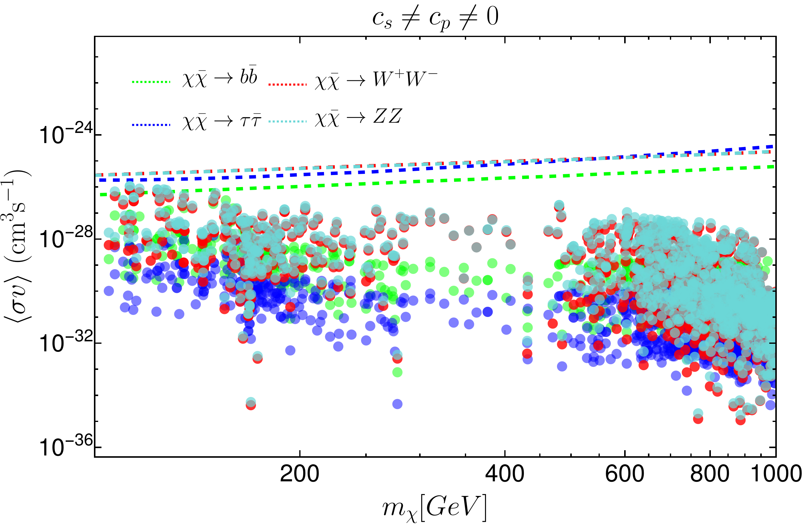
(a)

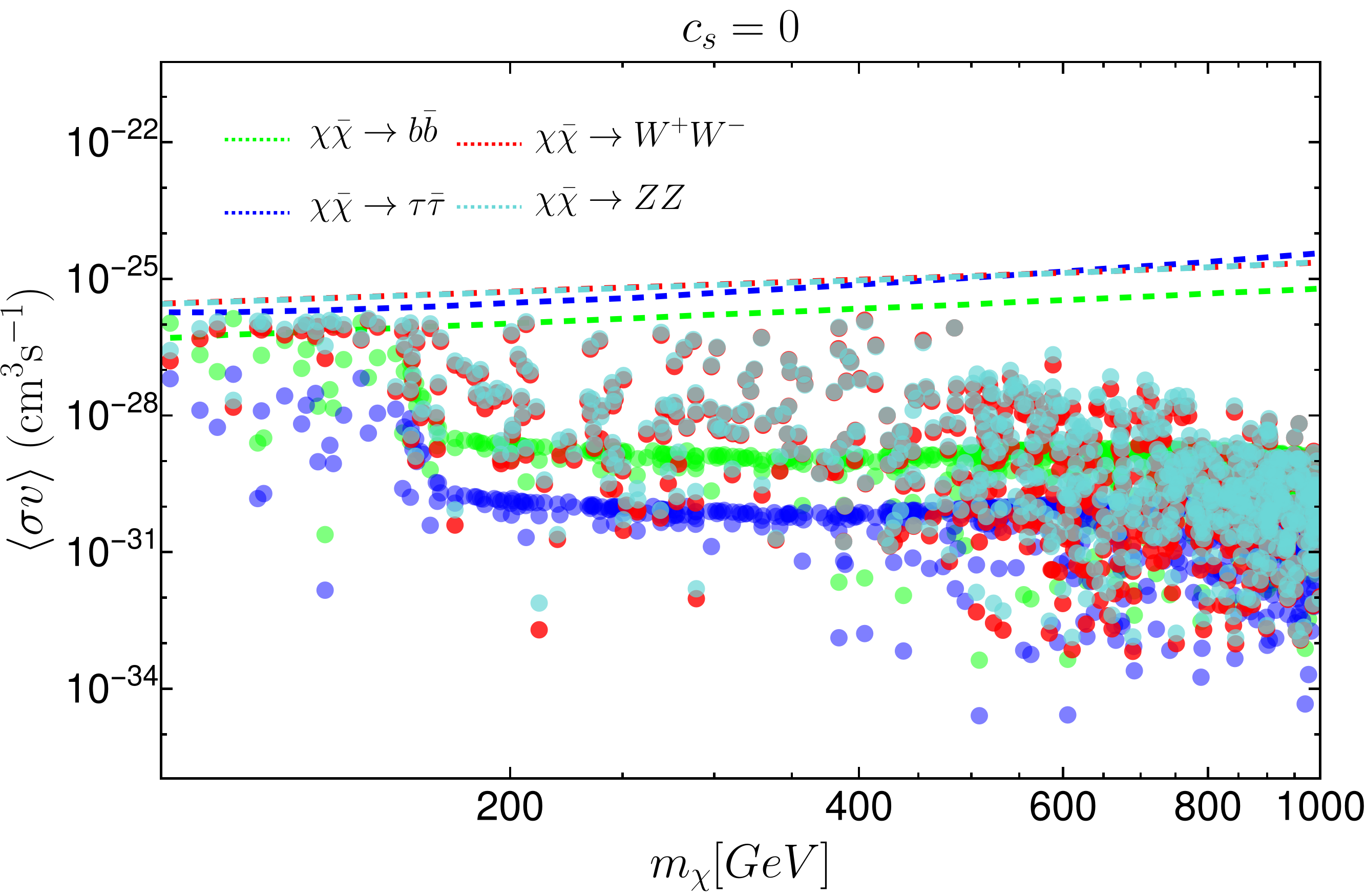
(b)

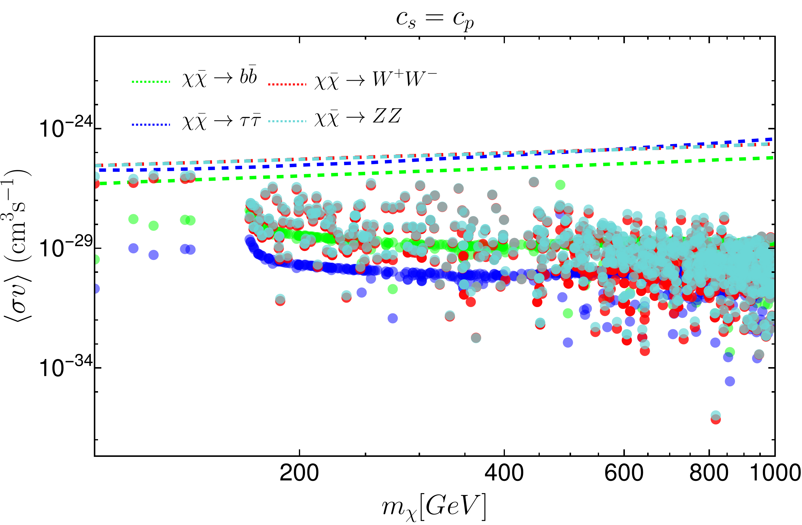
(c)

Figure 19: Variation of indirect detection cross-section of the DM with its mass $m_{\chi}.$ Plots are shown for different combinations of scalar and pseudoscalar couplings $c_{s}$ and $c_{p},$ i.e. for $c_{s}\neq c_{p}$ (upper left), $c_{s}=0$ (upper right) and $c_{s}=c_{p}$ (lower). The dashed lines are observational DM annihilation cross-sections bound to SM channels mentioned in the inset of the plot, whereas the same colour scatter plots correspond to the annihilation rate for our model to that channel. Points are allowed from both DM relic and DD cross-section as well as other observables mentioned in table 4.

In fig 19, we have shown the parameter space in $<\sigma v>-m_{\chi}$ plane for the annihilation rate of DM to boson and fermionic pair. The green colour corresponds to $\chi\bar{\chi}\to b\bar{b}$, blue colour corresponds to $\chi\bar{\chi}\to\tau\bar{\tau}$, red corressponds to $\chi\bar{\chi}\to W^{+}W^{-}$ and finally cyan shows $\chi\bar{\chi}\to ZZ$ bounds. In each plot, all the scatter points correspond to one particular color, showing the annihilation cross-section rate to that particular channel for this model. Also, all the points in the plot satisfy both observed relic density value and direct detection cross-section bounds along with all other flavour and electroweak observables. Figs. 19a , 19b and 19c shows the annihilation rate for different coupling combinations of $c_{s}$ and $c_{p}.$ The upper-left panel plot is done where $c_{s},~{}c_{p}$ both are free and varied freely. The plot in the upper right panel is done for the case when there is only pseudoscalar coupling between the mediator and SM, i.e., $c_{s}=0.$ The last plot in the lower panel is done when both the couplings are there, but they are equal, i.e., $c_{s}=c_{p}.$ In each plot, the dashed lines denote the bound of the corresponding annihilation channel given by Fermi-Lat, mentioned earlier. For the higher mass region, all the points lie well below the provided bound, but for the lower mass region, we get a comparable bound from our model.

We can see from the figures that the parameter space, which was allowed by DM relic density, direct detection, and of the flavour, electroweak observables, are also allowed by indirect detection bound provided by Fermi-LAT. Indirect detection bound does not exclude or give better constraints in the parameter space.

5.2 Bounds on the dimensionless couplings

In our analysis, we have obtained bounds on the dimensionful couplings: $c_{s},~{}c_{p}$ and $c_{G}$ which are related to the dimensionless couplings $g_{s},~{}g_{p}$ and $g_{V}$, respectively, via the relations given in eqs. (7) and (8). The bounds on the dimensionful couplings from the FCNC, FCCC and electroweak precesion observables are as follows:

$$|c_{s}|\lesssim 0.01\rm~{}GeV^{-1},\quad|c_{p}|\lesssim 0.01\rm~{}GeV^{-1},\quad|c_{G}|\lesssim 0.002\rm~{}GeV^{-1}.$$ (93)

Using these bounds we obtain the following bounds on the dimensionless couplings

$$|g_{s}|\lesssim 1.74,\quad|g_{p}|\lesssim 1.74,\quad|g_{V}|\lesssim 0.49.$$ (94)

However, while we include the data on DM relic density, direct and indirect detection bounds the above bounds will depend on $m_{\chi},~{}c_{s\chi}$ and $c_{p\chi}$. If we take $m_{\chi}\geq 500$ GeV and $c_{s\chi}\geq 0.1,~{}c_{p\chi}\geq 0.1$, the bounds on $c_{s},~{}c_{p}$ will be : $|c_{s}|,~{}|c_{p}|\lesssim 0.005\rm~{}GeV^{-1}$ which will lead to :

$$|g_{s}|\lesssim 0.87,\quad|g_{p}|\lesssim 0.87.$$ (95)

However, one should note that, $c_{s}$ and $c_{p}$ has a correlation which we have pointed out earlier. If we take $c_{s\chi},c_{p\chi}\geq 0.5$ the corresponding bounds will be $c_{s},~{}c_{p}\lesssim 0.001\rm~{}GeV^{-1}$ which will lead to :

$$|g_{s}|\lesssim 0.17,\quad|g_{p}|\lesssim 0.17.$$ (96)

For $m_{\chi}<500$ GeV, the bounds will be little relaxed even if we take $c_{s\chi}$ and $c_{p\chi}>0.1$ and the relevant bounds will follow eq. (95). The bounds on $g_{V}$ will not depend on the data on DM searches and the relevant bound will the eq. (94).

In section 2.1.2, we have shown an example of a toy model with dim-5 operators from which we can formulate our working model. We can see from eq. (2.1.2) that for small mixing angle, the relation between the couplings of the toy model and our working model will be as follows:

$$\mathbb{C}_{s}^{S}=m_{f}~{}c_{s}=-\frac{C~{}v~{}\alpha}{\Lambda\sqrt{2}},\quad\mathbb{C}_{p}^{S}=m_{f}~{}c_{p}=-\frac{C~{}v}{\Lambda\sqrt{2}}\,,$$ (97)

and

$$\mathbb{C}_{W}^{S}=\frac{C^{\prime}m_{W}^{2}}{\Lambda},\quad\mathbb{C}_{Z}^{S}=\frac{C^{\prime}m_{Z}^{2}}{2\Lambda}\,.$$ (98)

Using eq. (97), we can estimate the value of $\alpha$ as:

$$\alpha=\frac{\mathbb{C}_{s}^{S}}{\mathbb{C}_{p}^{S}}\,.$$ (99)

Hence, using the bounds on $c_{s},~{}c_{p}$ and $c_{G}$ we have obtained

$$\left|\frac{C^{{}^{\prime}}}{\Lambda}\right| ~{}\approx~{} 2c_{G}~{}\leq 0.004\rm~{}GeV^{-1},$$ (100)

$$\left|\frac{C}{\Lambda\sqrt{2}}\right| ~{}\approx~{} \frac{c_{p}~{}m_{t}}{v}~{}\leq 0.007\rm~{}GeV^{-1}\,.$$ (101)

Here, we have only used the coupling with the top quark to compare the couplings, but we can also use the other fermion couplings, which will be little relaxed.

6 Summary

We have considered a simplified DM model with a fermionic dark matter and a spin-0 mediator communicating to the SM fermions and gauge bosons. We obtain the constraints on the scalar and pseudoscalar couplings of the mediator with the SM fermions ($c_{s},c_{p}$) and the new gauge couplings ($c_{G}$) from a simultaneous analysis of the inputs associated with the measurements of the low energy FCCC and FCNC observables, $W$ and $Z$-pole observables and the bounds on $t\to bW$ effective couplings. Among the low-energy FCCC observables, we have considered the inputs on the CKM matrix, as well as semileptonic and leptonic rates. The FCNC observables include the available data on semileptonic, leptonic, and rare decays corresponding to $b\to s\ell^{+}\ell^{-}$, $s\to d\ell^{+}\ell^{-}$ and $c\to u\ell^{+}\ell^{-}$ transitions and the available limits on the branching fraction of the invisible decays $P\to P^{\prime}\nu\bar{\nu}$. In addition, we have considered the inputs on oscillation amplitudes on the $B_{d/s}-\bar{B}_{d/s}$, $K-\bar{K}$ and $D_{0}-\bar{D}_{0}$ mixings. We have varied $M_{S}$ over 100 GeV to 1000 GeV. In the unit of GeV^-1, we find the following constraints: $|c_{s}|\lesssim 0.01\rm~{}GeV^{-1}$, $|c_{p}|\lesssim 0.01\rm~{}GeV^{-1}$ and $|c_{G}|\lesssim 0.002\rm~{}GeV^{-1}$. To get these numbers, we have not included the data on $W$ mass measurement from CDF, which shows deviation with respect to the other respective data. If we include this data, then the required value of the gauge coupling will be $|c_{G}|\approx 0.004$ GeV^-1.

Finally, from a simultaneous analysis of these data sets alongside the data on DM relic density and direct detection cross section we find out the allowed parameter spaces for the DM mass ($m_{\chi}$), mediator mass ($M_{S}$), the couplings ($c_{s}$, $c_{p}$) and the couplings ($c_{s\chi}$, $c_{p\chi}$) of the DM with the mediator. Also, we have shown the correlations between these parameters and noted that for the DM mass $m_{\chi}>500$ GeV and $c_{p\chi}\gtrsim 0.1$, the allowed values are $|c_{s}|\lesssim 0.005$ GeV^-1 and $|c_{p}|\lesssim 0.005$ GeV^-1. Both the values independently will be even less than $0.001$ GeV^-1 if we take $c_{p\chi}\gtrsim 0.5$. We obtain these solutions within the allowed region $0.01<c_{s\chi}\lesssim 1.0$. For $m_{\chi}<400$ GeV, the constraints on $|c_{s}|$ and $|c_{p}|$ will be little relaxed but both of them will be $\lesssim 0.005$ GeV^-1 when $c_{p\chi}\gtrsim 0.1$. Similarly, we have obtained strong correlations between $c_{s\chi}$, $c_{s}$ and $M_{S}$. We have noted that for $M_{S}<500$ GeV, the bound on $|c_{s}|$ will be highly constrained ($\lesssim 0.005$ GeV^-1) and this bound will reduce further for $c_{s\chi}\gtrsim 0.1$. For $M_{S}\gtrsim 500$ GeV, we will obtain $|c_{s}|\lesssim 0.1$ GeV^-1 and will gradually reduce as $c_{s\chi}$ increases towards a value $\approx 1.0$.

Note:

We have provided the final correlated data set obtained from our combined analysis, named DM_flavor_2TeV.dat, which could be useful for collider and other relevant analysis.

Appendix

Appendix A Higher dimensional model

Couplings with Fermions :

Starting from the higher dimensional Lagrangian

$$\mathcal{L}_{ferm}=-\frac{C}{\Lambda}[\bar{\Psi}_{L}i\gamma_{5}H\psi_{R}P]-y_{f}[\bar{\psi}_{L}H\psi_{R}]+h.c,$$ (102)

with

$$H=\begin{pmatrix}0\\ \frac{v+h}{\sqrt{2}}\end{pmatrix}\quad\text{and}\quad P=u+S_{1}.$$

$u$ and $v$ are the VEV corresponding to the doublet $H$ and singlet $P.$ By expanding the Lagrangian (for the down quark only),

$$\mathcal{L}_{ferm}= -\frac{C}{\Lambda}\left[\bar{d}_{L}i\gamma_{5}\left(\frac{v+h}{\sqrt{2}}\right)d_{R}(u+S_{1})\right]-y_{f}\left[\bar{d}_{L}\left(\frac{v+h}{\sqrt{2}}\right)d_{R}\right]+h.c$$

$$\Rightarrow-\bar{d}\left[\frac{y_{f}}{\sqrt{2}}+i\frac{Cuv}{\sqrt{2}\Lambda}\gamma_{5}\right]d+\left[..\text{interaction terms}..\right]$$ (103)

We need to perform a chiral transformation to absorb the $\gamma_{5}$ part of the mass to get the mass basis.

$$\psi\to e^{\frac{i\gamma_{5}\alpha}{2}}\psi,\quad\psi_{L}\to e^{-\frac{i\alpha}{2}}\psi_{L},\quad\psi_{R}\to e^{\frac{i\alpha}{2}}\psi_{R},$$ (104)

where

$$\tan\alpha=\frac{Cuv}{y_{f}\Lambda}.$$

With this rotation of the fermionic field, we get the correct mass term. The fermionic bilinears will be transformed as:

$$\begin{split}\bar{\psi}i\gamma_{5}\psi\to\bar{\psi}i\gamma_{5}\psi-\alpha\bar{\psi}\psi\,,\\ \bar{\psi}\psi\to\bar{\psi}\psi+\alpha\bar{\psi}i\gamma_{5}\psi\,.\end{split}$$ (105)

Using this Chiral transformation, the dimension four interaction terms can be written as:

$$-i\left(\frac{Cu}{\Lambda\sqrt{2}}+\frac{y_{f}}{\sqrt{2}}\right)[\bar{d}\gamma_{5}dh]-\left(\frac{y_{f}}{\sqrt{2}}-\frac{Cu\alpha}{\Lambda\sqrt{2}}\right)\left[\bar{d}dh\right]\\ -i\left(\frac{Cv}{\Lambda\sqrt{2}}\right)\left[\bar{d}dS_{1}\right]\,.$$ (106)

Now, another rotation of basis needs to be performed to get the scalars in mass basis by angle $\theta$, such that:

$$\begin{split}h_{1}=\cos\theta~{}h-\sin\theta~{}S_{1}\,,\\ S=\sin\theta~{}h+\cos\theta~{}S_{1}\,,\end{split}$$ (107)

with $h_{1}$ and $S$ being the SM scalar and new scalar, respectively. They are in mass basis. Using this the kinetic mixing of scalars in the above eq. (106), we get the interaction terms of the scalars with down quark pairs as:

$$\begin{split}-\left[\left(\frac{y_{f}}{\sqrt{2}}-\frac{Cu\alpha}{\Lambda\sqrt{2}}\right)\cos\theta+\frac{Cv\alpha}{\Lambda\sqrt{2}}\sin\theta\right]\left[\bar{d}dh_{1}\right]-i\left[\left(\frac{Cu}{\Lambda\sqrt{2}}+\frac{y_{f}}{\sqrt{2}}\right)\cos\theta-\frac{Cv}{\Lambda\sqrt{2}}\sin\theta\right]\left[\bar{d}\gamma_{5}dh_{1}\right]\\ -\left[\left(\frac{y_{f}}{\sqrt{2}}-\frac{Cu\alpha}{\Lambda\sqrt{2}}\right)\sin\theta-\frac{Cv\alpha}{\Lambda\sqrt{2}}\cos\theta\right]\left[\bar{d}dS\right]-i\left[\left(\frac{Cu}{\Lambda\sqrt{2}}+\frac{y_{f}\alpha}{\sqrt{2}}\right)\sin\theta-\frac{Cv}{\Lambda\sqrt{2}}\cos\theta\right]\left[\bar{d}\gamma_{5}dS\right]\end{split}$$ (108)

Gauge boson couplings:

Starting from the higher dimensional Lagrangian

$$\mathcal{L}_{gauge}=\frac{C^{\prime}}{\Lambda}S|D_{\mu}H|^{2}+|D_{\mu}H|^{2},$$ (109)

We get interactions with the SM Higgs as well as the new scalar. After expanding the above interaction terms and giving basis rotation to the scalars to get them in mass basis as in eq. (107), the interaction terms can be written as:

$$\begin{split}\mathcal{L}_{gauge}=\left(\frac{2m_{W}^{2}}{v}\cos\theta-\frac{C^{\prime}m_{W}^{2}}{\Lambda}\sin\theta\right)[W_{\mu}^{+}W^{\mu-}h_{1}]+\left(\frac{m_{Z}^{2}}{v}\cos\theta-\frac{C^{\prime}m_{Z}^{2}}{2\Lambda}\sin\theta\right)[Z_{\mu}Z^{\mu}h_{1}]\\ +\left(\frac{2m_{W}^{2}}{v}\sin\theta+\frac{C^{\prime}m_{W}^{2}}{\Lambda}\cos\theta\right)[W_{\mu}^{+}W^{\mu-}S]+\left(\frac{m_{Z}^{2}}{v}\sin\theta+\frac{C^{\prime}m_{Z^{2}}}{2\Lambda}\cos\theta\right)[Z_{\mu}Z^{\mu}S]\end{split}$$ (110)

Appendix B FCNC vertex correction

We have written in eqs. (2.2.1) and (2.2.1), the FCNC loop contribution coming from Feynman diagrams fig. 1 in terms of loop functions $I$’s. The expressions for $I_{1}$ and $I_{2}$ coming from fig. 1a, are given by as following:

$$\begin{split}I_{1}=&\int_{0}^{1}dx\int_{0}^{1-x}dy\biggl{\{}\frac{m_{t}^{2}}{m_{W}^{2}}\biggl{(}c_{s}(1-2x)-ic_{p}\biggr{)}+\frac{m_{t}^{2}}{\Delta^{2}}2\biggl{(}-c_{s}(1+2x)+ic_{p}\biggr{)}\\ &+\frac{m_{t}^{2}}{m_{W}^{2}}\frac{1}{\Delta^{2}}\biggl{(}m_{d_{i}}^{2}x^{2}\biggl{(}c_{s}(1-2x)+ic_{p}\biggr{)}\biggr{)}+\frac{m_{t}^{2}}{m_{W}^{2}}\biggl{(}c_{s}(1+6x)+ic_{p}\biggr{)}\log\frac{m_{t}^{2}}{\Delta^{2}}\biggr{\}}\,,\end{split}$$ (111)

$$I_{2} =\int_{0}^{1}dx\int_{0}^{1-x}dy\biggl{\{}\frac{m_{t}^{2}}{m_{W}^{2}}\biggl{(}-c_{s}(1+2y)+ic_{p}\biggr{)}+2\frac{m_{t}^{2}}{\Delta^{2}}\biggl{(}c_{s}(1-2y)-ic_{p}\biggr{)}$$

$$+\frac{m_{t}^{2}}{m_{W}^{2}\Delta^{2}}\biggl{(}m_{d_{i}}^{2}x^{2}\biggl{(}-c_{s}(1+2y)+ic_{p}\biggr{)}+2m_{d_{i}}^{2}xy(c_{s}+ic_{p})\biggr{)}+\frac{m_{t}^{2}}{m_{W}^{2}}\biggl{(}c_{s}(1+6y)-ic_{p}\biggr{)}\log\frac{m_{t}^{2}}{\Delta^{2}}\biggr{\}}\,,$$ (112)

Where, $\Delta^{2}=xm_{W}^{2}+(1-x)m_{t}^{2},$ for $I_{1}$ and $I_{2}$. Loop functions $I_{3}$ and $I_{4}$ coming from fig. 1b, are given by:

$$I_{3}= \frac{c_{G}}{2m_{W^{2}}}\int_{0}^{1}dx\int_{0}^{1-x}dy\frac{1}{\Delta^{2}}\biggl{\{}2\Delta^{2}\Big{[}4m_{W}^{2}(3x+3y-1)-3\Delta^{2}(8x+8y-3)\Big{]}\log\left(\frac{m_{W}^{2}}{\Delta^{2}}\right)$$

$$+4m_{d_{i}}^{2}m_{W}^{2}\left(x(1-y+xy)-y(1+y+y^{2})+\frac{y-2}{2}\right)-8\Delta^{2}(x+y)$$

$$+\Delta^{2}m_{d_{i}}^{2}\left(x(x+y)-4y(1+x^{2}-y^{2})\right)-4\Delta^{4}(5x+5y-3)-8m_{W}^{4}(x+y-1)\biggr{\}}\,,$$ (113)

$$I_{4}= \frac{c_{G}}{4m_{W^{2}}}\int_{0}^{1}dx\int_{0}^{1-x}dy\frac{1}{\Delta^{2}}\biggl{\{}4\Delta^{2}\bigg{[}4m_{W^{2}}(2-3y)-3\Delta^{2}(5-8y)\bigg{]}\log\left(\frac{m_{W}^{2}}{\Delta^{2}}\right)$$

$$+2(1-y)\bigg{[}\Delta^{2}m_{d_{i}}^{2}(x-4xy+4y^{2})-2m_{W}^{2}\bigg{]}$$

$$+16ym_{W}^{4}-8\Delta^{4}(2-5y)\biggr{\}}\,.$$ (114)

Where, $\Delta^{2}=xm_{t}^{2}+(1-x)m_{W}^{2}$ for $I_{3}$ and $I_{4}.$

Appendix C Additional inputs for analysis

In section 4.1, we have discussed the fit results of our model parameters $c_{s},c_{p},c_{G}$ and $M_{S}$ from the analysis of relevant FCNC, FCCC, $W$ and $Z$ pole observables. The observables considered are given in table 4. The additional inputs that are also taken in fit are given below in table 8.

Input Parameters	Value	Reference
$f_{+}^{K\to\pi}(0)$	$0.9706(27)$	$N_{f}=2+1+1$ FLAG:2019
$f_{K^{\pm}}/f_{\pi^{\pm}}$	$1.1973(08)(14)$	Average CKMFitter:2021
$f_{K}$	$155.7(3)$	$N_{f}=2+1+1$ FLAG:2021
$f_{+}^{DK}(0)$	$0.7385(44)$	$N_{f}=2+1+1$ FLAG:2021
$f_{+}^{D\pi}(0)$	$0.621(18)(12)$	AverageCKMFitter:2021
$f_{B_{s}}$	$230.3(1.3)$ MeV	$N_{f}=2+1+1$ FLAG:2021
$f_{B_{s}}/f_{B}$	$1.209(5)$	$N_{f}=2+1+1$ FLAG:2021
$B_{K}$	$0.7625(97)$	$N_{f}=2+1$ FLAG:2021
$f_{D_{s}}$	$249.9(5)$ MeV	$N_{f}=2+1+1$ FLAG:2021
$f_{D_{s}}/f_{D}$	$1.1783(16)$	$N_{f}=2+1+1$ FLAG:2021
$\zeta(\Lambda_{p}\to p\mu^{-}\bar{\nu}_{\mu})_{q^{2}>15}/\zeta(\Lambda_{p}\to\Lambda_{c}\mu^{-}\bar{\nu}_{\mu})_{q^{2}>7}$	$1.471(96)(0.290)$	CKMFitter:2021
$B_{B_{s}}$	$1.327(16)(30)$	Average CKMFitter:2021
$B_{B_{s}}/B_{B_{d}}$	$1.007(13)(14)$	Average CKMFitter:2021
$\bar{m}_{c}(m_{c})$	$1.2976(13)(120)$ GeV	Average CKMFitter:2021
$\bar{m}_{t}(m_{t})$	$165.26(11)(30)$ GeV	CKMFitter:2021
$\eta_{tt}$	$0.550(0)(024)$	CKMFitter:2021
$\eta_{ut}$	$0.402(0)(007)$	CKMFitter:2021
$\eta_{B}(\bar{\text{MS}})$	$0.5510(0)(22)$	CKMFitter:2021
$B_{2}$	$0.46(1)(3)$	$N_{f}=2+1+1$ FLAG:2021
$B_{4}$	$0.78(2)(4)$	$N_{f}=2+1+1$FLAG:2021

Table 8: List of aditional inputs used for the CKM fit with updated values of 2021-22.

Appendix D Fit results for $c_{s}=c_{p}$

In above section 4.1, we have shown the fit values of our model parameters $c_{s},~{}c_{p}$ and $c_{G}$ for the general case where: $c_{s}\neq c_{p},$ taking into account all the relevant flavour changing changed and neutral current processes with $W$ and $Z$ pole observables. Here, we have added the fit results for the case: $c_{s}=c_{p}$ in table 9.

$\Lambda$ [TeV]	$M_{S}$ $\rm[GeV]$	$c_{s}(=c_{p})\times 10$ $\rm[GeV^{-1}]$	$c_{G}\times 10^{3}$ $\rm[GeV^{-1}]$	$\Delta M_{W}\times 10^{2}$ $\rm[GeV]$
	$250$	$-0.0046\pm 0.1242$	$2.7703\pm 0.2585$	$4.6574\pm 0.8693$
	$500$	$-0.0079\pm 0.1375$	$-3.4324\pm 0.3214$	$4.6536\pm 0.8716$
$1$	$800$	$0.0261\pm 0.1717$	$4.4872\pm 0.4196$	$4.6450\pm 0.8688$
	$250$	$0.0066\pm 0.1048$	$-2.3046\pm 0.2158$	$4.6580\pm 0.8724$
	$500$	$0.0009\pm 0.1096$	$-2.6456\pm 0.2478$	$4.6557\pm 0.8721$
	$800$	$0.0052\pm 0.1166$	$3.0478\pm 0.2846$	$4.6528\pm 0.8691$
$2$	$1000$	$-0.0094\pm 0.1216$	$-3.3300\pm 0.3120$	$4.6504\pm 0.8714$

Table 9: Fit results of the parameters $c_{s}$ and $c_{G}$ for different combinations of $M_{S}$ and $\Lambda$ when $c_{s}=c_{p}$ is onsidered. All the observables, including $\delta(\Delta r)$ (CDF, LHCb, ATLAS, D0), are taken into account. The p-value for this fit is $\sim 3.59\%$ with 46 d.o.f. The last column shows the prediction of $\Delta M_{W}$ from this fit result.

$\Lambda$ [TeV]	$M_{S}$ $\rm[GeV]$	$c_{s}(=c_{p})\times 10$ $\rm[GeV^{-1}]$	$c_{G}\times 10^{3}$ $\rm[GeV^{-1}]$	$\Delta M_{W}\times 10^{2}$ $\rm[GeV]$
	$250$	$0.0014\pm 0.1241$	$-0.8202\pm 1.4140$	$0.4083\pm 1.4076$
	$500$	$-0.0024\pm 0.1382$	$-1.0125\pm 1.7567$	$0.4049\pm 1.4051$
$1$	$800$	$0.0085\pm 0.1548$	$1.3217\pm 2.2803$	$0.4030\pm 1.3905$
	$250$	$-0.0020\pm 0.1039$	$0.6834\pm 1.1601$	$0.4096\pm 1.3907$
	$500$	$-0.0003\pm 0.1105$	$0.7819\pm 1.3376$	$0.4066\pm 1.3913$
	$800$	$0.0016\pm 0.1174$	$0.8982\pm 1.5465$	$0.4041\pm 1.3915$
$2$	$1000$	$0.0029\pm 0.1215$	$0.9799\pm 1.6930$	$0.4026\pm 1.3914$

Table 10: Fit results of the couplings for different sets of $\Lambda$ and $M_{S}$ in the presence of both scalar and pseudoscalar coupling are equal, i.e., $c_{s}=c_{p}$. All the observables of table 4 are taken into account along with the weighted mean data of $\delta(\Delta r)$ observable from LHCb, ATLAS and D0 experiment LHCb:2021bjt ; ATLAS:2017rzl ; ATLAS:2023fsi ; D0:2012kms . The p-value of this fit is $\sim 34.36\%.$ with 43 d.o.f. The last column shows the prediction of $\Delta M_{W}$ from this fit result.

Appendix E Dark Matter

The expression for the cross-section of DM annihilating to SM fermion pair $(\bar{\chi}\chi\to\bar{f}f)$ is given by Berlin:2014tja :

$$\sigma v \approx \frac{N_{c}c_{p\chi}^{2}m_{f}^{2}\sqrt{1-m_{f}^{2}/m_{\chi}^{2}}\Big{[}m_{\chi}^{2}(c_{p}^{2}+c_{s}^{2})-m_{f}^{2}c_{s}^{2}\Big{]}}{2\pi\left(m_{A}^{2}-4m_{\chi}^{2}\right)^{2}}$$

$$+ \frac{N_{c}v^{2}}{16\pi m_{\chi}^{2}\left(4m_{\chi}^{2}-m_{A}^{2}\right)^{3}\sqrt{1-m_{f}^{2}/m_{\chi}^{2}}}\Bigg{[}c_{p\chi}^{2}\bigg{\{}c_{p}^{2}m_{f}^{2}m_{\chi}^{2}\Big{(}m_{A}^{2}(m_{f}^{2}-2m_{\chi}^{2})+12m_{f}^{2}m_{\chi}^{2}-8m_{\chi}^{4}\Big{)}$$

$$+ c_{s}^{2}m_{f}^{2}(m_{f}^{2}-m_{\chi}^{2})\Big{(}m_{A}^{2}(m_{f}^{2}+2m_{\chi}^{2})-20m_{f}^{2}m_{\chi}^{2}+8m_{\chi}^{4}\Big{)}\bigg{\}}$$

$$- 2c_{s\chi}^{2}m_{f}^{2}(m_{A}^{2}-4m_{\chi}^{2})(m_{\chi}^{2}-m_{f}^{2})\Big{(}m_{\chi}^{2}(c_{p}^{2}+c_{s}^{2})-m_{f}^{2}c_{s}^{2}\Big{)}\Bigg{]}.$$

Where, $N_{c}=3,$ for quarks and $N_{c}=1,$ for annihilation to lepton pairs.

The effective spin-independent nucleon-WIMP $(N-\chi)$ inelastic scattering cross-section in zero transfer momentum limit $(q^{2}\to 0)$, can be given by:

$$\sigma^{\rm SI}_{\chi N}\simeq\frac{\mu_{\chi N}^{2}c_{s\chi}^{2}}{\pi M_{S}^{4}}\left(Z\widetilde{f}_{p}+(A-Z)\widetilde{f}_{n}\right)^{2},$$ (116)

where, $\mu_{\chi N}$ is the reduced mass of DM-nuclei and $\widetilde{f}_{n}$ are defined below. The nucleon form factor is defined as :

$$\frac{\widetilde{f}_{n}}{m_{n}}= \sum_{q=u,d,s}f_{T_{q}}^{n}\,\frac{\widetilde{f}_{q}}{m_{q}}+\frac{2}{27}\,f_{TG}\sum_{q=c,b,t}\frac{\widetilde{f}_{q}}{m_{q}}\,,$$ (117)

$$\to\frac{m_{q}c_{s}}{GeV}\left(\frac{7}{9}\sum_{q=u,d,s}f_{T_{q}}^{n}+\frac{2}{9}\right),$$ (118)

where in the second line we take $\widetilde{f}_{q}=c_{s}m_{q}^{2}/{\rm GeV}$ and $f_{TG}=1-f^{n}_{T_{u}}-f^{n}_{T_{d}}-f^{n}_{T_{s}}$, with $f_{T_{u}}^{p(n)}=0.018(0.013)$ ,   $f_{T_{d}}^{p(n)}=0.027(0.040)$ and $f_{T_{s}}^{p(n)}=0.037(0.037)$ Bhattacharya:2017fid .

References

- (1) Y. Bai and J. Berger, Fermion Portal Dark Matter, JHEP 11 (2013) 171 [1308.0612].
- (2) D. Schmeier, Effective Models for Dark Matter at the International Linear Collider, other thesis, 8, 2013, [1308.4409].
- (3) M.R. Buckley, D. Feld and D. Goncalves, Scalar Simplified Models for Dark Matter, Phys. Rev. D 91 (2015) 015017 [1410.6497].
- (4) J. Abdallah et al., Simplified Models for Dark Matter and Missing Energy Searches at the LHC, 1409.2893.
- (5) J. Abdallah et al., Simplified Models for Dark Matter Searches at the LHC, Phys. Dark Univ. 9-10 (2015) 8 [1506.03116].
- (6) A. Berlin, S. Gori, T. Lin and L.-T. Wang, Pseudoscalar Portal Dark Matter, Phys. Rev. D 92 (2015) 015005 [1502.06000].
- (7) S. Baek, P. Ko, M. Park, W.-I. Park and C. Yu, Beyond the Dark matter effective field theory and a simplified model approach at colliders, Phys. Lett. B 756 (2016) 289 [1506.06556].
- (8) C. Englert, M. McCullough and M. Spannowsky, S-Channel Dark Matter Simplified Models and Unitarity, Phys. Dark Univ. 14 (2016) 48 [1604.07975].
- (9) A. Albert et al., Towards the next generation of simplified Dark Matter models, Phys. Dark Univ. 16 (2017) 49 [1607.06680].
- (10) A. De Simone and T. Jacques, Simplified models vs. effective field theory approaches in dark matter searches, Eur. Phys. J. C 76 (2016) 367 [1603.08002].
- (11) G. Arcadi, M. Dutra, P. Ghosh, M. Lindner, Y. Mambrini, M. Pierre et al., The waning of the WIMP? A review of models, searches, and constraints, Eur. Phys. J. C 78 (2018) 203 [1703.07364].
- (12) M. Bauer, M. Klassen and V. Tenorth, Universal properties of pseudoscalar mediators in dark matter extensions of 2HDMs, JHEP 07 (2018) 107 [1712.06597].
- (13) G. Arcadi, M. Lindner, F.S. Queiroz, W. Rodejohann and S. Vogl, Pseudoscalar Mediators: A WIMP model at the Neutrino Floor, JCAP 03 (2018) 042 [1711.02110].
- (14) D. Abercrombie et al., Dark Matter benchmark models for early LHC Run-2 Searches: Report of the ATLAS/CMS Dark Matter Forum, Phys. Dark Univ. 27 (2020) 100371 [1507.00966].
- (15) LHC Dark Matter Working Group collaboration, LHC Dark Matter Working Group: Next-generation spin-0 dark matter models, Phys. Dark Univ. 27 (2020) 100351 [1810.09420].
- (16) C. Arina, Impact of cosmological and astrophysical constraints on dark matter simplified models, Front. Astron. Space Sci. 5 (2018) 30 [1805.04290].
- (17) G. Arcadi, A. Djouadi and M. Raidal, Dark Matter through the Higgs portal, Phys. Rept. 842 (2020) 1 [1903.03616].
- (18) G. Arcadi, G. Busoni, T. Hugle and V.T. Tenorth, Comparing 2HDM Scalar and Pseudoscalar Simplified Models at LHC, JHEP 06 (2020) 098 [2001.10540].
- (19) G. Arcadi, A. Djouadi and M. Kado, The Higgs-portal for vector dark matter and the effective field theory approach: A reappraisal, Phys. Lett. B 805 (2020) 135427 [2001.10750].
- (20) M.J. Dolan, F. Kahlhoefer, C. McCabe and K. Schmidt-Hoberg, A taste of dark matter: Flavour constraints on pseudoscalar mediators, JHEP 03 (2015) 171 [1412.5174].
- (21) P. Harris, V.V. Khoze, M. Spannowsky and C. Williams, Constraining Dark Sectors at Colliders: Beyond the Effective Theory Approach, Phys. Rev. D 91 (2015) 055009 [1411.0535].
- (22) F. Kahlhoefer, K. Schmidt-Hoberg, T. Schwetz and S. Vogl, Implications of unitarity and gauge invariance for simplified dark matter models, JHEP 02 (2016) 016 [1510.02110].
- (23) M. Backović, M. Krämer, F. Maltoni, A. Martini, K. Mawatari and M. Pellen, Higher-order QCD predictions for dark matter production at the LHC in simplified models with s-channel mediators, Eur. Phys. J. C 75 (2015) 482 [1508.05327].
- (24) M.R. Buckley and D. Goncalves, Constraining the Strength and CP Structure of Dark Production at the LHC: the Associated Top-Pair Channel, Phys. Rev. D 93 (2016) 034003 [1511.06451].
- (25) O. Buchmueller, A. De Roeck, K. Hahn, M. McCullough, P. Schwaller, K. Sung et al., Simplified Models for Displaced Dark Matter Signatures, JHEP 09 (2017) 076 [1704.06515].
- (26) F. Kahlhoefer, K. Schmidt-Hoberg and S. Wild, Dark matter self-interactions from a general spin-0 mediator, JCAP 08 (2017) 003 [1704.02149].
- (27) E. Morgante, Simplified Dark Matter Models, Adv. High Energy Phys. 2018 (2018) 5012043 [1804.01245].
- (28) I.Z. Rothstein, TASI lectures on effective field theories, 8, 2003 [hep-ph/0308266].
- (29) A.V. Manohar, Introduction to Effective Field Theories, 1804.05863.
- (30) S. Matsumoto, Y.-L.S. Tsai and P.-Y. Tseng, Light Fermionic WIMP Dark Matter with Light Scalar Mediator, JHEP 07 (2019) 050 [1811.03292].
- (31) Y.G. Kim, K.Y. Lee and S. Shin, Singlet fermionic dark matter, JHEP 05 (2008) 100 [0803.2932].
- (32) C. Arina et al., A comprehensive approach to dark matter studies: exploration of simplified top-philic models, JHEP 11 (2016) 111 [1605.09242].
- (33) U. Haisch and E. Re, Simplified dark matter top-quark interactions at the LHC, JHEP 06 (2015) 078 [1503.00691].
- (34) A. Biswas, L. Mukherjee, S. Nandi and S.K. Patra, Constraining new physics with possible dark matter signatures from a global CKM fit, Phys. Rev. D 107 (2023) 055041 [2111.01176].
- (35) T. Li, Simplified dark matter models in the light of AMS-02 antiproton data, JHEP 04 (2017) 112 [1612.09501].
- (36) T. Li, Revisiting the direct detection of dark matter in simplified models, Phys. Lett. B 782 (2018) 497 [1804.02120].
- (37) A. Berlin, D. Hooper and S.D. McDermott, Simplified Dark Matter Models for the Galactic Center Gamma-Ray Excess, Phys. Rev. D 89 (2014) 115022 [1404.0022].
- (38) S. Ipek, D. McKeen and A.E. Nelson, A Renormalizable Model for the Galactic Center Gamma Ray Excess from Dark Matter Annihilation, Phys. Rev. D 90 (2014) 055021 [1404.3716].
- (39) J.M. No, Looking through the pseudoscalar portal into dark matter: Novel mono-Higgs and mono-Z signatures at the LHC, Phys. Rev. D 93 (2016) 031701 [1509.01110].
- (40) D. Goncalves, P.A.N. Machado and J.M. No, Simplified Models for Dark Matter Face their Consistent Completions, Phys. Rev. D 95 (2017) 055027 [1611.04593].
- (41) M. Bauer, U. Haisch and F. Kahlhoefer, Simplified dark matter models with two Higgs doublets: I. Pseudoscalar mediators, JHEP 05 (2017) 138 [1701.07427].
- (42) X. Liu, L. Bian, X.-Q. Li and J. Shu, Type-III two Higgs doublet model plus a pseudoscalar confronted with , muon and dark matter, Nucl. Phys. B 909 (2016) 507 [1508.05716].
- (43) A. DiFranzo, K.I. Nagao, A. Rajaraman and T.M.P. Tait, Simplified Models for Dark Matter Interacting with Quarks, JHEP 11 (2013) 014 [1308.2679].
- (44) S. Baek, P. Ko and W.-I. Park, Invisible Higgs Decay Width vs. Dark Matter Direct Detection Cross Section in Higgs Portal Dark Matter Models, Phys. Rev. D 90 (2014) 055014 [1405.3530].
- (45) A. Greljo, J. Julio, J.F. Kamenik, C. Smith and J. Zupan, Constraining Higgs mediated dark matter interactions, JHEP 11 (2013) 190 [1309.3561].
- (46) I. Boiarska, K. Bondarenko, A. Boyarsky, V. Gorkavenko, M. Ovchynnikov and A. Sokolenko, Phenomenology of GeV-scale scalar portal, JHEP 11 (2019) 162 [1904.10447].
- (47) B. Batell, M. Pospelov and A. Ritz, Multi-lepton Signatures of a Hidden Sector in Rare B Decays, Phys. Rev. D 83 (2011) 054005 [0911.4938].
- (48) M. Freytsis, Z. Ligeti and J. Thaler, Constraining the Axion Portal with , Phys. Rev. D 81 (2010) 034001 [0911.5355].
- (49) J.P. Saha and A. Kundu, Reevaluating bounds on flavor changing neutral current parameters in R parity conserving and R parity violating supersymmetry from B0 anti-B0 mixing, Phys. Rev. D 69 (2004) 016004 [hep-ph/0307259].
- (50) J.S. Hagelin, S. Kelley and T. Tanaka, Exact supersymmetric amplitude for K0 - anti-K0 and B0 - anti-B0 mixing, Mod. Phys. Lett. A 8 (1993) 2737 [hep-ph/9304218].
- (51) Fermilab Lattice, MILC collaboration, -mixing matrix elements from lattice QCD for the Standard Model and beyond, Phys. Rev. D 93 (2016) 113016 [1602.03560].
- (52) L. Di Luzio, M. Kirk, A. Lenz and T. Rauh, theory precision confronts flavour anomalies, JHEP 12 (2019) 009 [1909.11087].
- (53) Heavy Flavor Averaging Group, HFLAV collaboration, Averages of b-hadron, c-hadron, and -lepton properties as of 2021, Phys. Rev. D 107 (2023) 052008 [2206.07501].
- (54) Particle Data Group collaboration, Review of Particle Physics, PTEP 2022 (2022) 083C01.
- (55) LHCb collaboration, Test of lepton universality in beauty-quark decays, 2103.11769.
- (56) LHCb collaboration, Constraints on the Branching Fraction, Phys. Rev. Lett. 125 (2020) 231801 [2001.10354].
- (57) CDF collaboration, Measurements of the Angular Distributions in the Decays at CDF, Phys. Rev. Lett. 108 (2012) 081807 [1108.0695].
- (58) LHCb collaboration, Measurement of the asymmetry in decays, Phys. Rev. Lett. 111 (2013) 151801 [1308.1340].
- (59) LHCb collaboration, Differential branching fractions and isospin asymmetries of decays, JHEP 06 (2014) 133 [1403.8044].
- (60) LHCb collaboration, Test of lepton universality using decays, Phys. Rev. Lett. 113 (2014) 151601 [1406.6482].
- (61) LHCb collaboration, Angular analysis of the decay using 3 fb-1 of integrated luminosity, JHEP 02 (2016) 104 [1512.04442].
- (62) Belle collaboration, Lepton-Flavor-Dependent Angular Analysis of , Phys. Rev. Lett. 118 (2017) 111801 [1612.05014].
- (63) CMS collaboration, Measurement of angular parameters from the decay in proton-proton collisions at 8 TeV, Phys. Lett. B 781 (2018) 517 [1710.02846].
- (64) ATLAS collaboration, Angular analysis of decays in collisions at TeV with the ATLAS detector, JHEP 10 (2018) 047 [1805.04000].
- (65) LHCb collaboration, Angular Analysis of the Decay, Phys. Rev. Lett. 126 (2021) 161802 [2012.13241].
- (66) LHCb collaboration, Branching Fraction Measurements of the Rare and - Decays, Phys. Rev. Lett. 127 (2021) 151801 [2105.14007].
- (67) LHCb collaboration, Test of lepton universality in decays, Phys. Rev. Lett. 131 (2023) 051803 [2212.09152].
- (68) S. Bhattacharya, A. Biswas, S. Nandi and S.K. Patra, Exhaustive model selection in decays: Pitting cross-validation against the Akaike information criterion, Phys. Rev. D 101 (2020) 055025 [1908.04835].
- (69) A. Biswas, S. Nandi, S.K. Patra and I. Ray, New physics in decays with complex Wilson coefficients, Nucl. Phys. B 969 (2021) 115479 [2004.14687].
- (70) A.J. Buras, Theoretical review of physics, Nucl. Instrum. Meth. A 368 (1995) 1 [hep-ph/9509329].
- (71) D. Becirevic, N. Kosnik, F. Mescia and E. Schneider, Complementarity of the constraints on New Physics from and from decays, Phys. Rev. D 86 (2012) 034034 [1205.5811].
- (72) C. Bobeth, M. Misiak and J. Urban, Photonic penguins at two loops and dependence of , Nucl. Phys. B 574 (2000) 291 [hep-ph/9910220].
- (73) W. Altmannshofer, P. Ball, A. Bharucha, A.J. Buras, D.M. Straub and M. Wick, Symmetries and Asymmetries of Decays in the Standard Model and Beyond, JHEP 01 (2009) 019 [0811.1214].
- (74) M. Beneke, C. Bobeth and R. Szafron, Power-enhanced leading-logarithmic QED corrections to , JHEP 10 (2019) 232 [1908.07011].
- (75) A.J. Buras, F. De Fazio, J. Girrbach, R. Knegjens and M. Nagai, The Anatomy of Neutral Scalars with FCNCs in the Flavour Precision Era, JHEP 06 (2013) 111 [1303.3723].
- (76) E949, E787 collaboration, Measurement of the K+ – pi+ nu nu branching ratio, Phys. Rev. D 77 (2008) 052003 [0709.1000].
- (77) BaBar collaboration, Search for the Rare Decay , Phys. Rev. D 82 (2010) 112002 [1009.1529].
- (78) Belle collaboration, Search for decays with semileptonic tagging at Belle, Phys. Rev. D 96 (2017) 091101 [1702.03224].
- (79) KOTO collaboration, Study of the Decay at the J-PARC KOTO Experiment, Phys. Rev. Lett. 126 (2021) 121801 [2012.07571].
- (80) D. Becirevic and A.B. Kaidalov, Comment on the heavy — light form-factors, Phys. Lett. B 478 (2000) 417 [hep-ph/9904490].
- (81) (HPQCD collaboration)§, HPQCD collaboration, B→K and D→K form factors from fully relativistic lattice QCD, Phys. Rev. D 107 (2023) 014510 [2207.12468].
- (82) R.R. Horgan, Z. Liu, S. Meinel and M. Wingate, Lattice QCD calculation of form factors describing the rare decays and , Phys. Rev. D 89 (2014) 094501 [1310.3722].
- (83) CMS, ATLAS collaboration, Combination of the W boson polarization measurements in top quark decays using ATLAS and CMS data at 8 TeV, JHEP 08 (2020) 051 [2005.03799].
- (84) CMS collaboration, Measurement of CKM matrix elements in single top quark -channel production in proton-proton collisions at 13 TeV, Phys. Lett. B 808 (2020) 135609 [2004.12181].
- (85) ATLAS collaboration, Measurement of the W boson polarisation in events from pp collisions at = 8 TeV in the lepton + jets channel with ATLAS, Eur. Phys. J. C 77 (2017) 264 [1612.02577].
- (86) CMS collaboration, Measurement of the W boson helicity fractions in the decays of top quark pairs to lepton jets final states produced in pp collisions at 8TeV, Phys. Lett. B 762 (2016) 512 [1605.09047].
- (87) Particle Data Group collaboration, Review of Particle Physics, PTEP 2022 (2022) 083C01.
- (88) D.A. Ross and M.J.G. Veltman, Neutral Currents in Neutrino Experiments, Nucl. Phys. B 95 (1975) 135.
- (89) M.J.G. Veltman, Limit on Mass Differences in the Weinberg Model, Nucl. Phys. B 123 (1977) 89.
- (90) M.S. Chanowitz, M.A. Furman and I. Hinchliffe, Weak Interactions of Ultraheavy Fermions. 2., Nucl. Phys. B 153 (1979) 402.
- (91) J. van der Bij and M.J.G. Veltman, Two Loop Large Higgs Mass Correction to the rho Parameter, Nucl. Phys. B 231 (1984) 205.
- (92) M.E. Peskin and T. Takeuchi, Estimation of oblique electroweak corrections, Phys. Rev. D 46 (1992) 381.
- (93) CDF collaboration, High-precision measurement of the boson mass with the CDF II detector, Science 376 (2022) 170.
- (94) LHCb collaboration, Measurement of the W boson mass, JHEP 01 (2022) 036 [2109.01113].
- (95) ATLAS collaboration, Improved W boson Mass Measurement using 7 TeV Proton-Proton Collisions with the ATLAS Detector, .
- (96) D0 collaboration, Measurement of the W Boson Mass with the D0 Detector, Phys. Rev. Lett. 108 (2012) 151804 [1203.0293].
- (97) A. Soni, A.K. Alok, A. Giri, R. Mohanta and S. Nandi, SM with four generations: Selected implications for rare B and K decays, Phys. Rev. D 82 (2010) 033009 [1002.0595].
- (98) J. Bernabeu, A. Pich and A. Santamaria, Top quark mass from radiative corrections to the Z — b anti-b decay, Nucl. Phys. B 363 (1991) 326.
- (99) A.E. Carcamo Hernandez, R. Martinez and F. Ochoa, Z and Z’ decays with and without FCNC in 331 models, Phys. Rev. D 73 (2006) 035007 [hep-ph/0510421].
- (100) R. Martinez and F. Ochoa, Constraints on 3-3-1 models with electroweak Z pole observables and Z’ search at the LHC, Phys. Rev. D 90 (2014) 015028 [1405.4566].
- (101) J. Bernabeu, D. Comelli, A. Pich and A. Santamaria, Hard m(t) corrections as a probe of the symmetry breaking sector, Phys. Rev. Lett. 78 (1997) 2902 [hep-ph/9612207].
- (102) J. Papavassiliou and A. Santamaria, Extra dimensions at the one loop level: Z — b anti-b and B anti-B mixing, Phys. Rev. D 63 (2001) 016002 [hep-ph/0008151].
- (103) A. Freitas, Higher-order electroweak corrections to the partial widths and branching ratios of the Z boson, JHEP 04 (2014) 070 [1401.2447].
- (104) SLD collaboration, Direct measurements of A(b) and A(c) using vertex/kaon charge tags at SLD, Phys. Rev. Lett. 94 (2005) 091801 [hep-ex/0410042].
- (105) SLD collaboration, Direct measurement of leptonic coupling asymmetries with polarized Zs, Phys. Rev. Lett. 79 (1997) 804 [hep-ex/9704012].
- (106) D. d’Enterria and V. Jacobsen, Improved strong coupling determinations from hadronic decays of electroweak bosons at N3LO accuracy, 2005.04545.
- (107) ATLAS collaboration, Test of the universality of and lepton couplings in -boson decays with the ATLAS detector, Nature Phys. 17 (2021) 813 [2007.14040].
- (108) CMS collaboration, Precision measurement of the W boson decay branching fractions in proton-proton collisions at = 13 TeV, Phys. Rev. D 105 (2022) 072008 [2201.07861].
- (109) S.K. Patra, OptEx, 2019.
- (110) L. Xayavong and N. Smirnova, Radial overlap correction to superallowed nuclear decays using the shell model with Hartree-Fock radial wave functions, Phys. Rev. C 105 (2022) 044308 [2111.13531].
- (111) The CKM Fitter Group collaboration, UPDATED RESULTS ON THE CKM MATRIX, .
- (112) A. Biswas, S. Nandi and I. Ray, Extractions of |Vub|/|Vcb| from a combined study of the exclusive decays, JHEP 07 (2023) 024 [2212.02528].
- (113) S. Jaiswal, S. Nandi and S.K. Patra, Extraction of from and the Standard Model predictions of , JHEP 12 (2017) 060 [1707.09977].
- (114) LHCb collaboration, Determination of the quark coupling strength using baryonic decays, Nature Phys. 11 (2015) 743 [1504.01568].
- (115) LHCb collaboration, Precise determination of the – oscillation frequency, Nature Phys. 18 (2022) 1 [2104.04421].
- (116) HFLAV collaboration, Averages of b-hadron, c-hadron, and -lepton properties as of 2018, Eur. Phys. J. C 81 (2021) 226 [1909.12524].
- (117) LHCb collaboration, Analysis of Neutral B-Meson Decays into Two Muons, Phys. Rev. Lett. 128 (2022) 041801 [2108.09284].
- (118) ATLAS collaboration, Measurement of the -boson mass in pp collisions at TeV with the ATLAS detector, Eur. Phys. J. C 78 (2018) 110 [1701.07240].
- (119) XENON collaboration, First Dark Matter Search with Nuclear Recoils from the XENONnT Experiment, Phys. Rev. Lett. 131 (2023) 041003 [2303.14729].
- (120) LZ collaboration, First Dark Matter Search Results from the LUX-ZEPLIN (LZ) Experiment, Phys. Rev. Lett. 131 (2023) 041002 [2207.03764].
- (121) PandaX collaboration, A search for dark matter-nucleon interactions with a dark mediator in PandaX-4T, 2308.01540.
- (122) Fermi-LAT collaboration, Searching for Dark Matter Annihilation from Milky Way Dwarf Spheroidal Galaxies with Six Years of Fermi Large Area Telescope Data, Phys. Rev. Lett. 115 (2015) 231301 [1503.02641].
- (123) Fermi-LAT collaboration, Sensitivity Projections for Dark Matter Searches with the Fermi Large Area Telescope, Phys. Rept. 636 (2016) 1 [1605.02016].
- (124) H.E.S.S. collaboration, Search for dark matter annihilations towards the inner Galactic halo from 10 years of observations with H.E.S.S, Phys. Rev. Lett. 117 (2016) 111301 [1607.08142].
- (125) H. Silverwood, C. Weniger, P. Scott and G. Bertone, A realistic assessment of the CTA sensitivity to dark matter annihilation, JCAP 03 (2015) 055 [1408.4131].
- (126) Flavour Lattice Averaging Group collaboration, FLAG Review 2019: Flavour Lattice Averaging Group (FLAG), Eur. Phys. J. C 80 (2020) 113 [1902.08191].
- (127) Flavour Lattice Averaging Group (FLAG) collaboration, FLAG Review 2021, Eur. Phys. J. C 82 (2022) 869 [2111.09849].
- (128) S. Bhattacharya, P. Ghosh, T.N. Maity and T.S. Ray, Mitigating Direct Detection Bounds in Non-minimal Higgs Portal Scalar Dark Matter Models, JHEP 10 (2017) 088 [1706.04699].