Monotone inclusion methods for a class of second-order non-potential mean-field games

Abstract

We propose a monotone splitting algorithm for solving a class of second-order non-potential mean-field games. Following [1], we introduce a finite-difference scheme and observe that the scheme represents first-order optimality conditions for a primal-dual pair of monotone inclusions. Based on this observation, we prove that the finite-difference system obtains a solution that can be provably recovered by an extension of the celebrated primal-dual hybrid gradient (PDHG) algorithm.

Primary, 35Q89, 65M06, 35A15, 49N80; Secondary, 35Q91, 35Q93, 91A16, 93A15, 93A16

1 Introduction

The main goal of the paper is to introduce a new algorithm for computing the solutions of the following system of PDE

(1) $$\begin{cases}-\partial_{t}\phi-\nu\Delta\phi+H(t,x,\nabla\phi,\rho)=f(t,x,\rho),\\ \partial_{t}\rho-\nu\Delta\rho-\nabla\cdot\left(\rho\nabla_{q}H(t,x,\nabla\phi,\rho)\right)=0,\\ \rho(0,x)=\rho_{0}(x),\quad\phi(T,x)=g(x,\rho(T,\cdot)).\end{cases}$$

Here, we assume periodic boundary conditions; that is, $(t,x)\in[0,T]\times\mathbb{T}^{d}$, where $\mathbb{T}^{d}=\mathbb{R}^{d}/\mathbb{Z}^{d}$ is the $d$-dimensional flat torus. Furthermore, $\nu\geq 0$ is the noise (viscosity) parameter, $H$ is the Hamiltonian, $f$ is the mean-field coupling function, and $g$ is the terminal cost function.

System Eq. 1 characterizes an equilibrium configuration for a continuum of agents that play a non-cooperative differential game. Such games are called mean-field games (MFG) and were independently introduced in [17, 18, 19] and [15, 14]. In this context, $\rho(t,x)$ and $\phi(t,x)$ are, respectively, the distribution and optimal cost of the agents at time $t$ and location $x$.

We introduce a numerical method for (1) in the spirit of Benamou-Brenier technique for solving optimal transportation and MFG systems [5, 6, 7, 9, 8]. In these works, the authors observe that when $H$ is separable; that is, $H(x,\rho,q)=H_{0}(x,q)-f(x,\rho)$, and suitable convexity, monotonicity, and structural assumptions are met, (1) can be seen as a first-order optimality condition for a convex-concave saddle-point problem. Such MFG are called variational or potential. Hence, one can use various convex optimization algorithms for computing the solutions of (1) such as the alternating direction method of multipliers (ADMM) [5, 6, 7] and primal-dual hybrid gradient (PDHG) [9, 8].

Here, we go beyond the potential and separable settings and provide a version of PDHG algorithm to solve (1). Our essential observation is that under the so-called Lasry-Lions monotonicity condition (1) can be seen as a primal-dual pair of monotone inclusions where the monotone maps are not subdifferential maps in general. We then solve (1) by a PDHG variant for monotone inclusions [22]. The possibility of solving non-potential MFG using monotone inclusion variants of PDHG was hinted on in [21] for nonlocal MFG systems.

For related work on non-separable MFG systems we refer to [20, 10] for policy iteration and Newton’s methods, and [3, 13, 12] for monotone flows. In [20, 10], the analyses strongly rely on the ellipticity and do not handle first-order systems ($\nu=0$) and non-smooth mean-field interactions ($\epsilon=0$ in Eq. 8). In contrast, we expect our methods to extend to these singular cases mutatis mutandis due to the variational nature of our techniques. Numerical experiments in Section 4.2 and Section 4.3 support our claim.

Works [3, 13, 12] address finite-state and stationary problems. Additionally, the algorithms in these works are forward only and do not come with convergence guarantees for the time-discretizations of the monotone flows.

2 Numerical analysis

2.1 A finite-difference scheme

We follow [1, 8] for introducing a semi-implicit scheme for (1). For simplicity, we assume that $d=2$. Let $h,\Delta t>0$ be such that $N_{h}=\frac{1}{h}\in\mathbb{N}$ and $N_{T}=\frac{T}{\Delta t}\in\mathbb{N}$. We then introduce uniform space-time grids

$$x_{ij}=(ih,jh),\quad t_{k}=k\Delta t,\quad 0\leq i,j\leq N_{h}-1,~{}0\leq k\leq N_{T}.$$

To enforce periodicity, we assume that $x_{ij}=x_{i^{\prime}j^{\prime}}$ whenever $i\equiv i^{\prime}~{}(\operatorname{mod}N_{h})$ and $j\equiv j^{\prime}~{}(\operatorname{mod}N_{h})$. Next, for a grid-function $f_{ij}^{k}=f(x_{ij},t_{k})$ we denote by

$$\begin{split}(D_{1}f^{k})_{ij}=&\frac{f^{k}_{(i+1)j}-f^{k}_{ij}}{h},\quad(D_{2}f^{k})_{ij}=\frac{f^{k}_{i(j+1)}-f^{k}_{ij}}{h},\\ &\\ [D_{h}f^{k}]_{ij}=&\left((D_{1}f^{k})_{ij},(D_{1}f^{k})_{(i-1)j},(D_{2}f^{k})_{ij},(D_{2}f^{k})_{i(j-1)}\right),\\ &\\ (\Delta_{h}f^{k})_{ij}=&\frac{f^{k}_{(i-1)j}+f^{k}_{(i+1)j}+f^{k}_{i(j-1)}+f^{k}_{i(j+1)}-4f^{k}_{ij}}{4h^{2}},\\ &\\ (D_{t}f_{ij})^{k}=&\frac{f_{ij}^{k+1}-f_{ij}^{k}}{\Delta t}.\end{split}$$

We then introduce a discretization of the Hamiltonian $H_{h}(t,x,q_{1},q_{2},q_{3},q_{4},\rho)$ that satisfies the following conditions

• Monotonicity: $H_{h}$ is nonincreasing in $q_{1},q_{3}$ and nondecreasing in $q_{2},q_{4}$.

• Consistency: $H_{h}(t,x,q_{1},q_{1},q_{2},q_{2},\rho)=H(t,x,q,\rho)$ for all $t\in[0,T]$, $x\in\mathbb{T}^{2}$, $\rho\geq 0$, and $q=(q_{1},q_{2})\in\mathbb{R}^{2}$.

• Differentiability: $\nabla_{q}H_{h}$ is continuous.

• Convexity: $(q_{1},q_{2},q_{3},q_{4})\mapsto H_{h}(t,x,q_{1},q_{2},q_{3},q_{4},\rho)$ is convex.

• Lasry-Lions monotonicity: A structural condition that yields existence and uniqueness of solutions of (1) is the so called Lasry-Lions monotonicity; that is,

  (2) $$\begin{pmatrix}-\partial_{\rho}H(t,x,q,\rho)&\frac{\rho\nabla_{q}^{\top}H(t,x,q,\rho)}{2}\\ \frac{\rho\nabla_{q}H(t,x,q,\rho)}{2}&\rho\nabla^{2}_{q}H(t,x,q,\rho)\end{pmatrix}\geq 0,$$

  for all $t\in[0,T]$, $(x,q)\in\mathbb{T}^{2}\times\mathbb{R}^{2}$, $\rho\geq 0$. We require the same condition on the discretized Hamiltonian; that is,

  (3) $$\begin{pmatrix}-\partial_{\rho}H_{h}(t,x,q_{1},q_{2},q_{3},q_{4},\rho)&\frac{\rho\nabla_{q}^{\top}H(t,x,q_{1},q_{2},q_{3},q_{4},\rho)}{2}\\ \frac{\rho\nabla_{q}H(t,x,q_{1},q_{2},q_{3},q_{4},\rho)}{2}&\rho\nabla^{2}_{q}H(t,x,q_{1},q_{2},q_{3},q_{4},\rho)\end{pmatrix}\geq 0,$$

  for all $t\in[0,T]$, $(x,q_{1},q_{2},q_{3},q_{4})\in\mathbb{T}^{2}\times\mathbb{R}^{4}$, $\rho\geq 0$.

With these ingredients at hand, the discretization of (1) introduced in [1] reads as follows:

(4) $$\begin{cases}-(D_{t}\phi_{ij})^{k}-\nu(\Delta_{h}\phi^{k})_{ij}+H_{h}(t_{k},x_{ij},[D_{h}\phi^{k}]_{ij},\rho_{ij}^{k+1})=f(t_{k},x_{ij},\rho^{k+1}_{ij})\\ (D_{t}\rho_{ij})^{k}-\nu(\Delta_{h}\rho^{k+1})_{ij}-\mathcal{B}_{ij}(t_{k},\phi^{k},\rho^{k+1},\rho^{k+1})=0,\\ \rho^{0}_{ij}=(\rho_{0})_{ij},~{}\phi^{N_{T}}_{ij}=g(x_{ij},\rho^{N_{T}}_{ij}),\quad 0\leq i,j\leq N_{h}-1,~{}0\leq k\leq N_{T}-1,\end{cases}$$

where

$$(\rho_{0})_{ij}=\frac{1}{h^{2}}\int\limits_{\|x-x_{ij}\|_{\infty}\leq h/2}\rho_{0}(x)dx.$$

and

$$\begin{split}&\mathcal{B}_{ij}(t,\phi,\rho,\eta)\\ =&\frac{1}{h}\left(\rho_{ij}\partial_{q_{1}}H_{h}(t,x_{ij},[D_{h}\phi]_{ij},\eta_{ij})-\rho_{(i-1)j}\partial_{q_{1}}H_{h}(t,x_{(i-1)j},[D_{h}\phi]_{(i-1)j},\eta_{(i-1)j})\right)\\ +&\frac{1}{h}\left(\rho_{(i+1)j}\partial_{q_{2}}H_{h}(t,x_{(i+1)j},[D_{h}\phi]_{(i+1)j},\eta_{(i+1)j})-\rho_{ij}\partial_{q_{2}}H_{h}(t,x_{ij},[D_{h}\phi]_{ij},\eta_{ij})\right)\\ +&\frac{1}{h}\left(\rho_{ij}\partial_{q_{3}}H_{h}(t,x_{ij},[D_{h}\phi]_{ij},\eta_{ij})-\rho_{i(j-1)}\partial_{q_{3}}H_{h}(t,x_{i(j-1)},[D_{h}\phi]_{i(j-1)},\eta_{i(j-1)})\right)\\ +&\frac{1}{h}\left(\rho_{i(j+1)}\partial_{q_{4}}H_{h}(t,x_{i(j+1)},[D_{h}\phi]_{i(j+1)},\eta_{i(j+1)})-\rho_{ij}\partial_{q_{4}}H_{h}(t,x_{ij},[D_{h}\phi]_{ij},\eta_{ij})\right).\end{split}$$

2.2 A discrete energy

Our goal is to formulate the discrete system (4) as a primal-dual pair of monotone inclusions. Following [8], we denote by $\mathcal{M}=\mathbb{R}^{(N_{T}+1)\times N_{h}\times N_{h}}$, $\mathcal{W}=(\mathbb{R}^{4})^{N_{T}\times N_{h}\times N_{h}}$, $\mathcal{U}=\mathbb{R}^{N_{T}\times N_{h}\times N_{h}}$ and introduce operators $A:\mathcal{M}\to\mathcal{U}$, $B:\mathcal{W}\to\mathcal{U}$ as follows:

$$\begin{split}(A\rho)^{k}_{ij}=&(D_{t}\rho_{ij})^{k}-\nu(\Delta\rho^{k+1})_{ij},\\ (Bw)^{k}_{ij}=&(D_{1}w^{k,1})_{(i-1)j}+(D_{1}w^{k,2})_{ij}+(D_{2}w^{k,3})_{i(j-1)}+(D_{2}w^{k,4})_{ij},\end{split}$$

for $0\leq i,j\leq N_{h}-1$ and $0\leq k\leq N_{T}-1$. Direct calculations [1, 8] show that

$$\begin{split}(B^{*}\phi)^{k}_{ij}=&-[D_{h}\phi^{k}]_{ij},\quad 0\leq k\leq N_{T}-1,\\ (A^{*}\phi)^{0}_{ij}=&-\frac{1}{\Delta t}\phi^{0}_{ij},\\ (A^{*}\phi)^{k}_{ij}=&-(D_{t}\phi_{ij})^{k-1}-\nu(\Delta_{h}\phi^{k-1})_{ij},\quad 1\leq k\leq N_{T}-1,\\ (A^{*}\phi)^{N_{T}}_{ij}=&\frac{\phi^{N_{T}-1}_{ij}}{\Delta t}-\nu(\Delta_{h}\phi^{N_{T}-1})_{ij}.\end{split}$$

Furthermore, we denote by $L_{h}$ the Legendre dual of $H_{h}$ defined as

(5) $$L_{h}(t,x,v_{1},v_{2},v_{3},v_{4},\eta)=\sup_{q_{1},q_{2},q_{3},q_{4}}\left(-\sum_{i=1}^{4}q_{i}v_{i}-H_{h}(t,x,q_{1},q_{2},q_{3},q_{4},\eta)\right),$$

and denote by $E_{h}$ the perspective function [11] of $L_{h}$; that is,

(6) $$E_{h}(t,x,\rho,w,\eta)=\begin{cases}\rho L_{h}\left(t,x,\frac{w}{\rho},\eta\right),\quad\rho>0,\\ (\operatorname{rec}L_{h}(t,x,\cdot,\eta))(w),\quad\rho=0,\\ \infty,\quad\text{otherwise},\end{cases}$$

where the recession function $\operatorname{rec}L_{h}(t,x,\cdot,\eta)$ is defined as

$$(\operatorname{rec}L_{h}(t,x,\cdot,\eta))(w)=\lim\limits_{s\to\infty}\frac{L_{h}(t,x,v_{0}+sw,\eta)}{s}.$$

Above, $v_{0}\in\mathbb{R}^{4}$ is an arbitrary point such that $L_{h}(t,x,v_{0},\eta)<\infty$.

Next, we define $J:\mathcal{M}\times\mathcal{W}\times\mathcal{M}\to\mathbb{R}\cup\{\infty\}$ as follows:

(7) $$\begin{split}J(\rho,w,\eta)=&\sum\limits_{\begin{subarray}{c}0\leq i,j\leq N_{h}-1\\ 0\leq k\leq N_{T}-1\end{subarray}}E_{h}(t_{k},x_{ij},\rho^{k+1}_{ij},w^{k}_{ij},\eta^{k+1}_{ij})+\sum\limits_{\begin{subarray}{c}0\leq i,j\leq N_{h}-1\\ 0\leq k\leq N_{T}-1\end{subarray}}F(t_{k},x_{ij},\rho^{k+1}_{ij})\\ &+\frac{1}{\Delta t}\sum\limits_{0\leq i,j\leq N_{h}-1}G(x_{ij},\rho_{ij}^{N_{T}})+\mathbf{1}_{\rho^{0}=\rho_{0}},\end{split}$$

where $\partial_{\rho}F(t,x,\rho)=f(t,x,\rho)$, and $\partial_{\rho}G(x,\rho)=g(x,\rho)$. Additionally, $\mathbf{1}_{E}$ is the convex characteristic function defined as

$$\mathbf{1}_{E}(y)=\begin{cases}0,\quad y\in E,\\ \infty,\quad y\notin E.\end{cases}$$

Remark 2.1.

A remarkable property of perspective functions is that $E_{h}(t,x,\cdot,\cdot,\eta)$ is a convex lower semicontinuous function [11].

2.3 A congestion model

For concreteness, we consider the MFG model with congestion discussed in [2]. More specifically, assume that

(8) $$H(t,x,q,\eta)=\frac{|q|^{\beta}}{\beta(\eta+\epsilon)^{\alpha}},$$

for some $\epsilon>0$, and

(9) $$1<\beta\leq 2,\quad 0<\alpha\leq\frac{4(\beta-1)}{\beta}.$$

These conditions together with the monotonicity of $\rho\mapsto f(t,x,\rho)$ and $\rho\mapsto g(x,\rho)$, and suitable technical assumptions yield the existence and uniqueness of weak solutions for (1) as analyzed in [2].

Following [1, 8], we discretize $H$ in (8) as follows

(10) $$H_{h}(t,x,q_{1},q_{2},q_{3},q_{4},\eta)=\frac{((q_{1}^{-})^{2}+(q_{2}^{+})^{2}+(q_{3}^{-})^{2}+(q_{4}^{+})^{2})^{\beta/2}}{\beta(\eta+\epsilon)^{\alpha}}$$

and denote by $K=\mathbb{R}_{+}\times\mathbb{R}_{-}\times\mathbb{R}_{+}\times\mathbb{R}_{-}$.

Lemma 2.2.

Assume that $H_{h}$ is given by (10). Then for every $(t,x)\in\mathbb{R}\times\mathbb{T}^{d}$ and $\eta\geq 0$ we have that

(11) $$L_{h}(t,x,v_{1},v_{2},v_{3},v_{4},\eta)=\begin{cases}(\eta+\epsilon)^{\alpha(\beta^{\prime}-1)}\frac{(v_{1}^{2}+v_{2}^{2}+v_{3}^{2}+v_{4}^{2})^{\beta^{\prime}/2}}{\beta^{\prime}},\quad(v_{1},v_{2},v_{3},v_{4})\in K,\\ \infty,\quad\text{otherwise},\end{cases}$$

where $\beta^{\prime}=\frac{\beta}{\beta-1}$. Furthermore, we have that

(12) $$E_{h}(t,x,\rho,w,\eta)=\begin{cases}(\eta+\epsilon)^{\alpha(\beta^{\prime}-1)}\frac{|w|^{\beta^{\prime}}}{\beta^{\prime}\rho^{\beta^{\prime}-1}},\quad\rho>0,~{}w\in K,\\ 0,\quad(\rho,w)=(0,0),\\ \infty,\quad\text{otherwise},\end{cases}$$

where $w=(w_{1},w_{2},w_{3},w_{4})$.

Proof 2.3.

We start by computing $L_{h}$. Suppose that $(v_{1},v_{2},v_{3},v_{4})\notin K$; for instance, let $v_{1}<0$. Then we have that

$$\begin{split}L_{h}(t,x,v_{1},v_{2},v_{3},v_{4},\eta)\geq\sup_{q_{1}>0}\left(-q_{1}v_{1}-H_{h}(t,x,q_{1},0,0,0,\eta)\right)=\sup_{q_{1}>0}\left(-q_{1}v_{1}\right)=\infty.\end{split}$$

Now assume that $(v_{1},v_{2},v_{3},v_{4})\in K$. The first order optimality conditions in the concave program (5) yield

$$v_{i}=-\partial_{q_{i}}H_{h}(t,x,q_{1},q_{2},q_{3},q_{4},\eta),\quad 1\leq i\leq 4.$$

Furthermore, we have that

$$\begin{split}\partial_{q_{i}}H_{h}(t,x,q_{1},q_{2},q_{3},q_{4},\eta)=&-\frac{((q_{1}^{-})^{2}+(q_{2}^{+})^{2}+(q_{3}^{-})^{2}+(q_{4}^{+})^{2})^{\beta/2-1}}{(\eta+\epsilon)^{\alpha}}q_{i}^{-},\quad i=1,3,\\ \partial_{q_{i}}H_{h}(t,x,q_{1},q_{2},q_{3},q_{4},\eta)=&\frac{((q_{1}^{-})^{2}+(q_{2}^{+})^{2}+(q_{3}^{-})^{2}+(q_{4}^{+})^{2})^{\beta/2-1}}{(\eta+\epsilon)^{\alpha}}q_{i}^{+},\quad i=2,4.\end{split}$$

Hence, the first order optimality conditions yield

$$\begin{split}v_{i}=&\frac{((q_{1}^{-})^{2}+(q_{2}^{+})^{2}+(q_{3}^{-})^{2}+(q_{4}^{+})^{2})^{\beta/2-1}}{(\eta+\epsilon)^{\alpha}}q_{i}^{-}\geq 0,\quad i=1,3,\\ v_{i}=&-\frac{((q_{1}^{-})^{2}+(q_{2}^{+})^{2}+(q_{3}^{-})^{2}+(q_{4}^{+})^{2})^{\beta/2-1}}{(\eta+\epsilon)^{\alpha}}q_{i}^{+}\leq 0,\quad i=2,4,\end{split}$$

and

$$\begin{split}v_{1}^{2}+v_{2}^{2}+v_{3}^{2}+v_{4}^{2}=&\frac{((q_{1}^{-})^{2}+(q_{2}^{+})^{2}+(q_{3}^{-})^{2}+(q_{4}^{+})^{2})^{\beta-1}}{(\eta+\epsilon)^{2\alpha}},\\ -q_{1}v_{1}-q_{2}v_{2}-q_{3}v_{3}-q_{4}v_{4}=&\frac{((q_{1}^{-})^{2}+(q_{2}^{+})^{2}+(q_{3}^{-})^{2}+(q_{4}^{+})^{2})^{\beta/2}}{(\eta+\epsilon)^{\alpha}}.\end{split}$$

Therefore, we obtain

$$\begin{split}L_{h}(t,x,v_{1},v_{2},v_{3},v_{4})=&\left(1-\frac{1}{\beta}\right)\frac{((q_{1}^{-})^{2}+(q_{2}^{+})^{2}+(q_{3}^{-})^{2}+(q_{4}^{+})^{2})^{\beta/2}}{(\eta+\epsilon)^{\alpha}}\\ =&\left(1-\frac{1}{\beta}\right)\frac{(\eta+\epsilon)^{\frac{\alpha\beta}{\beta-1}}(v_{1}^{2}+v_{2}^{2}+v_{3}^{2}+v_{4}^{2})^{\frac{\beta}{2(\beta-1)}}}{(\eta+\epsilon)^{\alpha}}\\ =&(\eta+\epsilon)^{\alpha(\beta^{\prime}-1)}\frac{(v_{1}^{2}+v_{2}^{2}+v_{3}^{2}+v_{4}^{2})^{\beta^{\prime}/2}}{\beta^{\prime}}.\end{split}$$

Next, we need to compute the recession function of $L_{h}(t,x,\cdot,\eta)$. Since

$$L_{h}(t,x,0,0,0,0,\eta)=0,$$

we have that $v_{0}=(0,0,0,0)\in\operatorname{dom}L_{h}(t,x,\cdot,\eta)$, and so we can compute the recession function via

$$(\operatorname{rec}L_{h}(t,x,\cdot,\eta))(w)=\lim\limits_{s\to\infty}\frac{L_{h}(t,x,sw,\eta)}{s}.$$

Since $L_{h}(t,x,w,\eta)=\infty$ for $w\notin K$ we have that

$$(\operatorname{rec}L_{h}(t,x,\cdot,\eta))(w)=\infty,\quad\forall w\notin K.$$

Furthermore, for $w\in K$ we have that

$$\begin{split}(\operatorname{rec}L_{h}(t,x,\cdot,\eta))(w)=&\lim\limits_{s\to\infty}\frac{L_{h}(t,x,sw,\eta)}{s}=\lim\limits_{s\to\infty}(\eta+\epsilon)^{\alpha(\beta^{\prime}-1)}\frac{s^{\beta^{\prime}}|w|^{\beta^{\prime}}}{s}\\ =&\begin{cases}0,\quad w=0,\\ \infty,\quad w\neq 0.\end{cases}\end{split}$$

Summarizing, we find that

$$(\operatorname{rec}L_{h}(t,x,\cdot,\eta))(w)=\begin{cases}0,\quad w=0,\\ \infty,\quad w\neq 0,\end{cases}$$

and (12) follows readily.

In [2], the authors point out that conditions (9) yield that $H$ satisfies the Lasry-Lions monotonicity condition (2). Here, we show that $H_{h}$ preserves that property.

Lemma 2.4.

Let $H_{h}$ be as in (10), and (9) hold. Then $H_{h}$ satisfies the Lasry-Lions monotonicity condition (3).

Proof 2.5.

Denoting by

(13) $$\psi(q_{1},q_{2},q_{3},q_{4})=\frac{((q_{1}^{-})^{2}+(q_{2}^{+})^{2}+(q_{3}^{-})^{2}+(q_{4}^{+})^{2})^{\beta/2}}{\beta},$$

we have that

$$H_{h}(t,x,q,\rho)=(\rho+\epsilon)^{-\alpha}\psi(q),$$

where we denote by $q=(q_{1},q_{2},q_{3},q_{4})$. Then we have that

$$\begin{split}\partial_{\rho}H_{h}=-\alpha(\rho+\epsilon)^{-\alpha-1}\psi(q),\quad\nabla_{q}H_{h}=(\rho+\epsilon)^{-\alpha}\nabla\psi(q),\\ \rho\nabla_{q}\partial_{\rho}H_{h}=-\alpha\rho(\rho+\epsilon)^{-\alpha-1}\nabla\psi(q),\quad\rho\nabla^{2}_{q}H_{h}=\rho(\rho+\epsilon)^{\alpha}\nabla^{2}\psi(q).\end{split}$$

Hence, we have to prove that

$$\begin{pmatrix}\alpha(\rho+\epsilon)^{-\alpha-1}\psi(q)&-\frac{1}{2}\alpha\rho(\rho+\epsilon)^{-\alpha-1}\nabla^{\top}\psi(q)\\ -\frac{1}{2}\alpha\rho(\rho+\epsilon)^{-\alpha-1}\nabla\psi(q)&\rho(\rho+\epsilon)^{\alpha}\nabla^{2}\psi(q)\end{pmatrix}\geq 0$$

for all $\rho\geq 0$ and $q\in\mathbb{R}^{4}$. Note that the inequality is trivial when $\rho=0$ because $\psi(q)\geq 0$ for all $q\in\mathbb{R}^{4}$. Hence, we can assume that $\rho>0$. Factoring out a positive number $\alpha\rho(\rho+\epsilon)^{-\alpha-1}$ we arrive at an equivalent inequality

$$\begin{pmatrix}\frac{\psi(q)}{\rho}&-\frac{\nabla^{\top}\psi(q)}{2}\\ -\frac{\nabla\psi(q)}{2}&\frac{\rho+\epsilon}{\alpha}\nabla^{2}\psi(q)\end{pmatrix}\geq 0.$$

Since $\psi$ is convex, we have that $\nabla^{2}\psi(q)\geq 0$. Additionally, from (9) we have that

$$\frac{\rho+\epsilon}{\alpha}\geq\frac{\beta\rho}{4(\beta-1)},$$

and so it is sufficient to prove that

$$\begin{pmatrix}\frac{\psi(q)}{\rho}&-\frac{\nabla^{\top}\psi(q)}{2}\\ -\frac{\nabla\psi(q)}{2}&\frac{\beta\rho}{4(\beta-1)}\nabla^{2}\psi(q)\end{pmatrix}\geq 0.$$

Next, since the previous inequality must hold for all $q\in\mathbb{R}^{4}$, we obtain an equivalent statement if we replace $q$ by $\rho q$; that is,

$$\begin{pmatrix}\frac{\psi(\rho q)}{\rho}&-\frac{\nabla^{\top}\psi(\rho q)}{2}\\ -\frac{\nabla\psi(\rho q)}{2}&\frac{\beta\rho}{4(\beta-1)}\nabla^{2}\psi(\rho q)\end{pmatrix}\geq 0,\quad\forall\rho>0,~{}q\in\mathbb{R}^{4}.$$

Denoting by $\psi_{\rho}(q)=\frac{\psi(\rho q)}{\rho}$, we find that the previous expression is nothing but

$$\begin{pmatrix}\psi_{\rho}(q)&-\frac{\nabla^{\top}\psi_{\rho}(q)}{2}\\ -\frac{\nabla\psi_{\rho}(q))}{2}&\frac{\beta}{4(\beta-1)}\nabla^{2}\psi_{\rho}(q)\end{pmatrix}\geq 0,\quad\forall\rho>0,~{}q\in\mathbb{R}^{4}.$$

Furthermore, due to the homogeneity of $\psi$, we have that $\psi_{\rho}(q)=\rho^{\beta-1}\psi(q)$, and so

$$\begin{pmatrix}\psi_{\rho}(q)&-\frac{\nabla^{\top}\psi_{\rho}(q)}{2}\\ -\frac{\nabla\psi_{\rho}(q)}{2}&\frac{\beta}{4(\beta-1)}\nabla^{2}\psi_{\rho}(q)\end{pmatrix}=\rho^{\beta-1}\begin{pmatrix}\psi(q)&-\frac{\nabla^{\top}\psi(q)}{2}\\ -\frac{\nabla\psi(q)}{2}&\frac{\beta}{4(\beta-1)}\nabla^{2}\psi(q)\end{pmatrix}.$$

The latter means that we need to prove that

$$\begin{pmatrix}\psi(q)&-\frac{\nabla^{\top}\psi(q)}{2}\\ -\frac{\nabla\psi(q)}{2}&\frac{\beta}{4(\beta-1)}\nabla^{2}\psi(q)\end{pmatrix}\geq 0,\quad\forall q\in\mathbb{R}^{4}.$$

For every $(\xi,\chi)\in\mathbb{R}\times\mathbb{R}^{4}$ we have to prove that

$$\begin{split}&(\xi,\chi)^{\top}\begin{pmatrix}\psi(q)&-\frac{\nabla^{\top}\psi(q)}{2}\\ -\frac{\nabla\psi(q)}{2}&\frac{\beta}{4(\beta-1)}\nabla^{2}\psi(q)\end{pmatrix}(\xi,\chi)\\ =&\xi^{2}\psi(q)-\xi\nabla\psi(q)\cdot\chi+\frac{\beta}{4(\beta-1)}\chi^{\top}\nabla^{2}\psi(q)\chi\geq 0\end{split}$$

When $\psi(q)=0$ we have that $\nabla\psi(q)=0$, and the inequality follows from $\nabla^{2}\psi(q)\geq 0$. Hence, assuming that $\psi(q)>0$ and optimizing with respect to $\xi$, we obtain an equivalent inequality

$$-\frac{|\nabla\psi(q)\cdot\chi|^{2}}{4\psi(q)}+\frac{\beta}{4(\beta-1)}\chi^{\top}\nabla^{2}\psi(q)\chi\geq 0,$$

or

$$\chi^{\top}\left(\frac{\beta}{\beta-1}\psi(q)\nabla^{2}\psi(q)-\nabla\psi(q)\otimes\nabla\psi(q)\right)\chi\geq 0.$$

Denoting by

$$\tilde{q}=(-q_{1}^{-},q_{2}^{+},-q_{3}^{-},q_{4}^{+}),\quad\text{for}\quad q=(q_{1},q_{2},q_{3},q_{4}),$$

we have that

$$\begin{split}\nabla\psi(q)=|\tilde{q}|^{\beta-2}\tilde{q},\quad\nabla^{2}\psi(q)=(\beta-2)|\tilde{q}|^{\beta-4}\tilde{q}\otimes\tilde{q}+|\tilde{q}|^{\beta-2}M(q),\end{split}$$

where

$$M(q)=\operatorname{diag}(\operatorname{Hvs}(-q_{1}),\operatorname{Hvs}(q_{2}),\operatorname{Hvs}(-q_{3}),\operatorname{Hvs}(q_{4})),$$

and $\operatorname{Hvs}$ is the Heaviside step function. Hence we obtain that

$$\begin{split}&\frac{\beta}{\beta-1}\psi(q)\nabla^{2}\psi(q)-\nabla\psi(q)\otimes\nabla\psi(q)\\ =&\frac{\beta-2}{\beta-1}|\tilde{q}|^{2\beta-4}\tilde{q}\otimes\tilde{q}+\frac{1}{\beta-1}|\tilde{q}|^{2\beta-2}M(q)-|\tilde{q}|^{2\beta-4}\tilde{q}\otimes\tilde{q}\\ =&\frac{|\tilde{q}|^{2\beta-4}}{\beta-1}(|\tilde{q}|^{2}M(q)-\tilde{q}\otimes\tilde{q}),\end{split}$$

and therefore we need to prove that

$$\begin{split}&((q_{1}^{-})^{2}+(q_{2}^{+})^{2}+(q_{3}^{-})^{2}+(q_{4}^{+})^{2})\\ \times&(\chi_{1}^{2}\operatorname{Hvs}(-q_{1})+\chi_{2}^{2}\operatorname{Hvs}(q_{2})+\chi_{3}^{2}\operatorname{Hvs}(-q_{3})+\chi_{4}^{2}\operatorname{Hvs}(q_{4}))\\ \geq&(-q_{1}^{-}\chi_{1}+q_{2}^{+}\chi_{2}-q_{3}^{-}\chi_{3}+q_{4}^{+}\chi_{4})^{2}.\end{split}$$

The latter simply follows from the Cauchy-Schwarz inequality

$$\sum_{i=1}^{4}a_{i}^{2}\cdot\sum_{i=1}^{4}b_{i}^{2}\geq\left(\sum_{i=1}^{4}a_{i}b_{i}\right)^{2}$$

applied to

$$\begin{split}a_{1}=&-q_{1}^{-},~{}a_{2}=q_{2}^{+},~{}a_{3}=-q_{3}^{-},~{}a_{4}=q_{4}^{+},\\ b_{1}=&\chi_{1}\operatorname{Hvs}(-q_{1}),~{}b_{2}=\chi_{2}\operatorname{Hvs}(q_{2}),~{}b_{3}=\chi_{3}\operatorname{Hvs}(-q_{3}),~{}b_{4}=\chi_{4}\operatorname{Hvs}(q_{4}),\end{split}$$

and taking into account that

$$q^{-}\operatorname{Hvs}(-q)=q^{-},\quad q^{+}\operatorname{Hvs}(q)=q^{+},\quad\operatorname{Hvs}(q)^{2}=\operatorname{Hvs}(q),\quad\forall q\in\mathbb{R}.$$

This completes the proof.

2.4 Properties of the discrete energy

Here, we discuss key properties of the function $J$ defined in (7).

Lemma 2.6.

Assume that $\eta\geq 0$, and $F(t,x,\cdot)$, $G(x,\cdot)$ are convex and continuous for $\rho\geq 0$. Furthermore, for $(\lambda,y,z)\in\{0,1\}\times\mathcal{M}\times\mathcal{W}$ denote by

(14) $$J_{\lambda,y,z}(\rho,w,\eta)=\lambda\left(\frac{|\rho|^{2}}{2}-\rho\cdot y+\frac{|w|^{2}}{2}-w\cdot z\right)+J(\rho,w,\eta).$$

Then the following statements are true.

1. The convex program

   (15) $$\inf_{(1-\lambda)(A\rho+Bw)=0}J_{\lambda,y,z}(\rho,w,\eta)$$

   admits a minimizer for all $(\lambda,y,z)\in\{0,1\}\times\mathcal{M}\times\mathcal{W}$.

2. When $\nu>0$ and $\lambda=0$ all minimizers of (15) satisfy

   (16) $$\rho^{k+1}_{ij}>0,\quad\forall 0\leq i,j\leq N_{h}-1,~{}0\leq k\leq N_{T}-1.$$

Remark 2.7.

The convex program (15) is analogous to the problem $(P_{h,\Delta t})$ in [8] with the difference of having extra parameters $\lambda,y,z,\eta$. Hence, the proof techniques used in [8, Theorem 3.1] and auxiliary lemmas extend to setting of Lemma 2.6.

Remark 2.8.

The convex program (15) is a shorthand for considering two programs

$$\inf_{A\rho+Bw=0}J(\rho,w,\eta)$$

and

$$\inf_{\rho,w}\left\{\frac{|\rho|^{2}}{2}-\rho\cdot y+\frac{|w|^{2}}{2}-w\cdot z+J(\rho,w,\eta)\right\}$$

simultaneously. Both are important for our further analysis.

Proof 2.9 (Proof of Lemma 2.6).

1. We argue by the direct method of calculus of variations. Fix a triple $(\lambda,y,z)\in\{0,1\}\times\mathcal{M}\times\mathcal{W}$. According to [8, Lemma 3.1] there exists $(\tilde{\rho},\tilde{w})\in\mathcal{M}\times\mathcal{W}$ such that

   (17) $$\tilde{\rho}^{k+1}_{ij}>0,\quad\tilde{w}^{k}_{ij}\in\operatorname{int}(K),\quad\forall 0\leq i,j\leq N_{h}-1,~{}0\leq k\leq N_{T}-1,$$

   and

   (18) $$A\tilde{\rho}+B\tilde{w}=0,\quad\tilde{\rho}^{0}_{ij}=(\rho_{0})_{ij},\quad\forall 1\leq i,j\leq N_{h}-1.$$

   Hence, $J_{\lambda,y,z}(\tilde{\rho},\tilde{w},\eta)<\infty$, and so

   $$\inf_{(1-\lambda)(A\rho+Bw)=0}J_{\lambda,y,z}(\rho,w,\eta)\leq J_{\lambda,y,z}(\tilde{\rho},\tilde{w},\eta)<\infty.$$

   1. When $\lambda=0$, for every $(\rho,w)$ such that $\rho\geq 0$, $\rho^{0}=\rho_{0}$, and $A\rho+Bw=0$ one has that [8, Section 3]

      $$\sum_{0\leq i,j\leq N_{h}-1}\rho^{k}_{ij}=\frac{1}{h^{2}},\quad\forall 0\leq k\leq N_{T},$$

      and so

      (19) $$0\leq\rho^{k}_{ij}\leq\frac{1}{h^{2}},\quad\forall 0\leq i,j\leq N_{h}-1,~{}0\leq k\leq N_{T}.$$

      Thus, taking into account the continuity of $F,G$ and the fact that $E_{h}\geq 0$, we find that

      $$\inf_{(1-\lambda)(A\rho+Bw)=0}J_{\lambda,y,z}(\rho,w,\eta)=\inf_{A\rho+Bw=0}J(\rho,w,\eta)>-\infty.$$

   2. When $\lambda=1$, the convexity of $F(t,x,\cdot)$ and $G(t,x,\cdot)$ yields

      (20) $$\begin{split}F(t_{k},x_{ij},\rho^{k+1}_{ij})\geq&F(t_{k},x_{ij},1)+(\rho^{k+1}_{ij}-1)d^{k+1}_{ij}\\ G(x_{ij},\rho^{N_{T}}_{ij})\geq&G(x_{ij},1)+(\rho^{N_{T}}_{ij}-1)r_{ij}\end{split}$$

      for some $d^{k+1}_{ij}\in\partial_{\rho}F(t_{k},x_{ij},1)$ and $r_{ij}\in\partial_{\rho}G(x_{ij},1)$. Thus, applying $E_{h}\geq 0$ in combination with the Cauchy-Schwarz inequality, we obtain

      $$J_{1,y,z}(\rho,w,\eta)\geq\frac{|\rho|^{2}}{2}-\rho\cdot\tilde{y}+\frac{|w|^{2}}{2}-w\cdot z-c\geq-\frac{|\tilde{y}|^{2}}{2}-\frac{|z|^{2}}{2}-c,$$

      where

      (21) $$\begin{split}\tilde{y}^{k+1}_{ij}=&y^{k+1}_{ij}-d^{k+1}_{ij},\quad 0\leq k\leq N_{T}-2\\ \tilde{y}^{N_{T}}_{ij}=&y^{N_{T}}_{ij}-d^{N_{T}}_{ij}-r_{ij},\\ c=&\sum\limits_{\begin{subarray}{c}0\leq i,j\leq N_{h}-1\\ 0\leq k\leq N_{T}-1\end{subarray}}(d^{k+1}_{ij}-F(t_{k},x_{ij},1))\\ &+\frac{1}{\Delta t}\sum\limits_{0\leq i,j\leq N_{h}-1}(r^{N_{T}}_{ij}-G(x_{ij},1)).\end{split}$$

      Hence

      $$\inf_{(1-\lambda)(A\rho+Bw)=0}J_{\lambda,y,z}(\rho,w,\eta)=\inf_{\rho,w}J_{1}(\rho,w,\eta)>-\infty.$$

   
   

   From (a), (b) above, we find that the infimum in (15) is always finite. Let $(\rho_{n},w_{n})$ be a minimizing sequence for (15). Then we have that

   $$J_{\lambda,y,z}(\rho_{n},w_{n},\eta)\leq C,\quad\forall n\geq 1,$$

   for some $C>0$. Our goal is to show that the sequence $\left\{(\rho_{n},w_{n})\right\}$ is bounded and extract a convergent subsequence. Again, let us discuss two cases.

   1. When $\lambda=0$, taking into account (19) for $\rho_{n}$ and the continuity of $F,G$, we have that

      (22) $$\begin{split}E_{h}(t_{k},x_{ij},(\rho_{n})^{k+1}_{ij},(w_{n})^{k}_{ij},\eta^{k+1}_{ij})\leq\tilde{C},\end{split}$$

      for all $n\geq 1$, $0\leq i,j\leq N_{h}-1$, $0\leq k\leq N_{T}-1$, and some $\tilde{C}>0$. Hence if $(\rho_{n})^{k+1}_{ij}>0$ then

      (23) $$|(w_{n})^{k}_{ij}|\leq\left(\frac{\beta^{\prime}}{\epsilon^{\alpha(\beta^{\prime}-1)}}\left(\frac{1}{h^{2}}\right)^{\beta^{\prime}-1}\tilde{C}\right)^{\frac{1}{\beta}}.$$

      If $(\rho_{n})^{k+1}_{ij}=0$ then we necessarily have that $(w_{n})^{k}_{ij}=0$. Thus, in any case (23) holds for all $i,j,k$.

   2. Let $\lambda=1$, and $\tilde{y},c,d,r$ be as in (20) and (21). Then we have that

      $$\begin{split}C\geq&J_{1,y,z}(\rho_{n},w_{n},\eta)\geq\frac{|\rho_{n}|^{2}}{2}-\rho_{n}\cdot\tilde{y}+\frac{|w_{n}|^{2}}{2}-w_{n}\cdot z-c\\ \geq&\frac{|\rho_{n}|^{2}}{4}+\frac{|w_{n}|^{2}}{4}-|\tilde{y}|^{2}-|z|^{2}-c,\end{split}$$

      and so

      $$\frac{|\rho_{n}|^{2}}{4}+\frac{|w_{n}|^{2}}{4}\leq|\tilde{y}|^{2}+|z|^{2}+c+C,\quad\forall n\geq 1.$$

   
   

   Thus, for both cases $\lambda=0$ and $\lambda=1$ the minimizing sequence $\left\{(\rho^{n},w^{n})\right\}$ is precompact, and there exists a (subsequential) limit $(\rho^{*},w^{*})\in\mathcal{M}\times\mathcal{W}$. Since $\rho_{n}\geq 0$, $(\rho_{n})^{0}=\rho_{0}$ and $(1-\lambda)(A\rho_{n}+Bw_{n})=0$, we have that

   $$\rho^{*}\geq 0,\quad(\rho^{*})^{0}=\rho_{0},\quad(1-\lambda)(A\rho^{*}+Bw^{*})=0.$$

   Furthermore, taking into account the lower semicontinuity of $E_{h}(t,x,\cdot,\cdot,\eta)$ (see Remark 2.1) and the continuity of $F,G$ we obtain that

   $$J_{\lambda,y,z}(\rho^{*},w^{*},\eta)\leq\liminf_{n\to\infty}J_{\lambda,y,z}(\rho_{n},w_{n},\eta),$$

   and so $(\rho^{*},w^{*})$ is a minimizer for (15).

2. See the proof of the analogous statement in [8, Lemma 3.2].

Denote by

(24) $$\mathcal{P}_{0}=\left\{\eta\in\mathcal{M}~{}:~{}\eta\geq 0,~{}\eta^{0}=\rho_{0},~{}\sum_{0\leq i,j\leq N_{h}-1}\eta^{k}_{ij}=\frac{1}{h^{2}},~{}\forall 1\leq k\leq N_{T}\right\},$$

and

(25) $$\mathcal{P}_{1}=\left\{\eta\in\mathcal{M}~{}:~{}\eta\geq 0,~{}\eta^{0}=\rho_{0},~{}|\eta|^{2}\leq c_{1}\right\},$$

where

$$\begin{split}c_{1}=&4\Bigg{(}|\tilde{y}|^{2}+|z|^{2}+c+\frac{|\bar{\rho}|^{2}}{2}-\bar{\rho}\cdot y+\sum\limits_{\begin{subarray}{c}0\leq i,j\leq N_{h}-1\\ 0\leq k\leq N_{T}-1\end{subarray}}F(t_{k},x_{ij},1)\\ &+\frac{1}{\Delta t}\sum\limits_{0\leq i,j\leq N_{h}-1}G(x_{ij},1)\Bigg{)},\\ \bar{\rho}^{0}=&\rho_{0},\quad\bar{\rho}^{k+1}_{ij}=1,~{}\forall 0\leq k\leq N_{T}-1,\end{split}$$

and $\tilde{y},c,d,r$ are as in (20) and (21).

Furthermore, for $\eta\geq 0$ and $(\lambda,y,z)\in\{0,1\}\times\mathcal{M}\times\mathcal{W}$ denote by

(26) $$\mathcal{S}_{\lambda,y,z}(\eta)=\left\{\rho^{*}~{}:~{}\exists w^{*}\in\mathcal{W}~{}\text{s.t.}~{}(\rho^{*},w^{*})\in\underset{(1-\lambda)(A\rho+Bw)=0}{\operatorname{argmin}}J_{\lambda,y,z}(\rho,w,\eta)\right\}.$$

Lemma 2.10.

Assume that $F(t,x,\cdot)$ and $G(x,\cdot)$ are convex and continuous for $\rho\geq 0$, and $(\lambda,y,z)\in\{0,1\}\times\mathcal{M}\times\mathcal{W}$. Then the set valued map $\mathcal{S}_{\lambda,y,z}:\mathcal{P}_{\lambda}\rightrightarrows\mathcal{P}_{\lambda}$ admits a fixed point; that is, there exists $\rho^{*}\in\mathcal{P}_{\lambda}$ such that $\rho^{*}\in\mathcal{S}_{\lambda,y,z}(\rho^{*})$.

Proof 2.11.

Our strategy is to apply Kakutani’s fixed point theorem [16]. Hence, fix a triple $(\lambda,y,z)\in\{0,1\}\times\mathcal{M}\times\mathcal{W}$.

1. Lemma 2.6 yields that $\mathcal{S}_{\lambda,y,z}(\eta)\neq\emptyset$ for all $\eta\geq 0$.

   1. When $\lambda=0$, we have that for all $\rho^{*}\in\mathcal{S}_{\lambda,y,z}(\eta)$ there exists $w^{*}\in\mathcal{W}$ such that

      $$(\rho^{*},w^{*})\in\underset{A\rho+Bw=0}{\operatorname{argmin}}J(\rho,w,\eta).$$

      Hence, $\rho^{*}\in\mathcal{P}_{0}$, and so $\mathcal{S}_{0,y,z}(\eta)\subset\mathcal{P}_{0}$ for all $\eta\in\mathcal{P}_{0}$.

   2. When $\lambda=1$, we have that for all $\rho^{*}\in\mathcal{S}_{\lambda,y,z}(\eta)$ there exists $w^{*}\in\mathcal{W}$ such that

      $$(\rho^{*},w^{*})\in\underset{\rho,w}{\operatorname{argmin}}~{}J_{1,y,z}(\rho,w,\eta),$$

      and so

      $$J_{1,y,z}(\rho^{*},w^{*},\eta)\leq J_{1,y,z}(\bar{\rho},0,\eta).$$

      Hence, applying lower bounds on $J_{1,y,z}$ as in Lemma 2.6 we obtain

      $$\frac{|\rho^{*}|^{2}}{4}+\frac{|w^{*}|^{2}}{4}\leq|\tilde{y}|^{2}+|z|^{2}+c+J_{1,y,z}(\bar{\rho},0,\eta).$$

      Noting that

      $$\begin{split}&J_{1}(\bar{\rho},0,\eta)\\ =&\frac{|\bar{\rho}|^{2}}{2}-\bar{\rho}\cdot y+\sum\limits_{\begin{subarray}{c}0\leq i,j\leq N_{h}-1\\ 0\leq k\leq N_{T}-1\end{subarray}}F(t_{k},x_{ij},1)+\frac{1}{\Delta t}\sum\limits_{0\leq i,j\leq N_{h}-1}G(x_{ij},1),\end{split}$$

      we conclude that $\rho^{*}\in\mathcal{P}_{1}$, and so $\mathcal{S}_{1,y,z}(\eta)\subset\mathcal{P}_{1}$ for all $\eta\in\mathcal{P}_{1}$.

   
   

   Summarizing (a), (b) above, we conclude that $\mathcal{S}_{\lambda,y,z}(\eta)\subset\mathcal{P}_{\lambda}$ for all $\eta\in\mathcal{P}_{\lambda}$. Additionally, the convexity and continuity of $F(t,x,\cdot)$ and $G(x,\cdot)$ yield that $J_{\lambda,y,z}(\cdot,\cdot,\eta)$ is convex and lower semicontinuous, and so

   $$\underset{(1-\lambda)(A\rho+Bw)=0}{\operatorname{argmin}}J_{\lambda,y,z}(\rho,w,\eta)$$

   is a closed convex set. Thus, $\mathcal{S}_{\lambda,y,z}(\eta)$ is also closed and convex.

2. Assume that $\{(\eta_{n},\rho_{n})\}\subset\mathcal{P}_{\lambda}\times\mathcal{P}_{\lambda}$ is such that $\rho_{n}\in\mathcal{S}_{\lambda,y,z}(\eta_{n})$ for all $n\geq 1$, and

   $$\lim\limits_{n\to\infty}(\eta_{n},\rho_{n})=(\hat{\eta},\hat{\rho}).$$

   Since $\mathcal{P}_{\lambda}$ is compact, we have that $\hat{\eta}\in\mathcal{P}_{\lambda}$. Furthermore, let $w_{n}\in\mathcal{W}$ be such that

   $$(\rho_{n},w_{n})\in\underset{(1-\lambda)(A\rho+Bw)=0}{\operatorname{argmin}}J_{\lambda,y,z}(\rho,w,\eta_{n}).$$

   Fix a $(\tilde{\rho},\tilde{w})\in\mathcal{M}\times\mathcal{W}$ such that (17) and (18) hold. Then we have that

   $$J_{\lambda,y,z}(\rho_{n},w_{n},\eta_{n})\leq J_{\lambda,y,z}(\tilde{\rho},\tilde{w},\eta_{n}),\quad\forall n\geq 1.$$

   Furthermore, we have that

   $$\lim_{n\to\infty}J_{\lambda,y,z}(\tilde{\rho},\tilde{w},\eta_{n})=J_{\lambda,y,z}(\tilde{\rho},\tilde{w},\hat{\eta})<\infty.$$

   Hence, there exists $C>0$ such that

   $$-\lambda\left(\frac{|y|^{2}}{2}+\frac{|z|^{2}}{2}\right)+J(\rho_{n},w_{n},\eta_{n})\leq J_{\lambda,y,z}(\rho_{n},w_{n},\eta_{n})\leq C,\quad\forall n\geq 1,$$

   and so

   $$J(\rho_{n},w_{n},\eta_{n})\leq C+\lambda\left(\frac{|y|^{2}}{2}+\frac{|z|^{2}}{2}\right),\quad\forall n\geq 1.$$

   Since $\{\rho_{n}\}$ is a bounded sequence and $F(t,x,\cdot)$, $G(x,\cdot)$ are continuous, we obtain that

   (27) $$0\leq E_{h}(t_{k},x_{ij},(\rho_{n})^{k+1}_{ij},(w_{n})^{k}_{ij},(\eta_{n})^{k+1}_{ij})\leq\tilde{C},$$

   for $0\leq i,j\leq N_{h}-1$, $0\leq k\leq N_{T}-1$, and some $\tilde{C}>0$. Next, denote by

   $$\ell(v_{1},v_{2},v_{3},v_{4})=\begin{cases}\frac{(v_{1}^{2}+v_{2}^{2}+v_{3}^{2}+v_{4}^{2})^{\beta^{\prime}/2}}{\beta^{\prime}},\quad(v_{1},v_{2},v_{3},v_{4})\in K,\\ \infty,\quad\text{otherwise}.\end{cases}$$

   The corresponding recession function is then

   $$\tilde{\ell}(\rho,w_{1},w_{2},w_{3},w_{4})=\begin{cases}\frac{(w_{1}^{2}+w_{2}^{2}+w_{3}^{2}+w_{4}^{2})^{\beta^{\prime}/2}}{\beta^{\prime}\rho^{\beta^{\prime}-1}},\quad(w_{1},w_{2},w_{3},w_{4})\in K,\\ 0,\quad(\rho,w_{1},w_{2},w_{3},w_{4})=(0,0,0,0,0),\\ \infty,\quad\text{otherwise}.\end{cases}$$

   Note that for $\eta\geq 0$ we have that

   (28) $$\begin{split}L_{h}(t,x,v_{1},v_{2},v_{3},v_{4},\eta)=&(\eta+\epsilon)^{\alpha(\beta^{\prime}-1)}\ell(v_{1},v_{2},v_{3},v_{4}),\\ E_{h}(t,x,w_{1},w_{2},w_{3},w_{4},\eta)=&(\eta+\epsilon)^{\alpha(\beta^{\prime}-1)}\tilde{\ell}(\rho,w_{1},w_{2},w_{3},w_{4}).\end{split}$$

   Taking into account $\eta_{n}\geq 0$ and (27) we obtain

   (29) $$0\leq\tilde{\ell}((\rho_{n})^{k+1}_{ij},(w_{n})^{k}_{ij})\leq\frac{\tilde{C}}{\epsilon^{\alpha(\beta^{\prime}-1)}}.$$

   In particular, we find that (23) holds. Thus $\{(\rho_{n},w_{n})\}$ is precompact, and, possibly through a subsequence, we have that

   $$\lim_{n\to\infty}(\rho_{n},w_{n})=(\hat{\rho},\hat{w}).$$

   Hence, we have that

   $$\begin{split}\hat{\rho}^{0}=&\lim_{n\to\infty}(\rho_{n})^{0}=\rho_{0},\quad\hat{\rho}=\lim_{n\to\infty}\rho_{n}\geq 0,\\ (1-\lambda)(A\hat{\rho}+B\hat{w})=&\lim_{n\to\infty}(1-\lambda)(A\rho_{n}+Bw_{n})=0.\end{split}$$

   Additionally, using the lower semicontinuity of $\tilde{\ell}$, we find that

   $$\begin{split}&\liminf_{n\to\infty}E_{h}(t_{k},x_{ij},(\rho_{n})^{k+1}_{ij},(w_{n})^{k}_{ij},(\eta_{n})^{k+1}_{ij})\\ \geq&\liminf_{n\to\infty}((\eta_{n})^{k+1}_{ij}+\epsilon)^{\alpha(\beta^{\prime}-1)}\cdot\liminf_{n\to\infty}\tilde{\ell}((\rho_{n})^{k+1}_{ij},(w_{n})^{k}_{ij})\\ \geq&(\hat{\eta}^{k+1}_{ij}+\epsilon)^{\alpha(\beta^{\prime}-1)}\tilde{\ell}(\hat{\rho}^{k+1}_{ij},\hat{w}^{k}_{ij})=E_{h}(t_{k},x_{ij},\hat{\rho}^{k+1}_{ij},\hat{w}^{k}_{ij},\hat{\eta}^{k+1}_{ij}),\end{split}$$

   for all $0\leq i,j\leq N_{h}-1$, and $0\leq l\leq N_{T}-1$. But then we have that

   $$\begin{split}&\liminf_{n\to\infty}J_{\lambda,y,z}(\rho_{n},w_{n},\eta_{n})\\ \geq&\liminf_{n\to\infty}\lambda\left(\frac{|\rho_{n}|^{2}}{2}-\rho_{n}\cdot y+\frac{|w_{n}|^{2}}{2}-w_{n}\cdot z\right)\\ &+\sum_{\begin{subarray}{c}0\leq i,j\leq N_{h}-1\\ 0\leq k\leq N_{T}-1\end{subarray}}\liminf_{n\to\infty}E_{h}(t_{k},x_{ij},(\rho_{n})^{k+1}_{ij},(w_{n})^{k}_{ij},(\eta_{n})^{k+1}_{ij})\\ &+\sum_{\begin{subarray}{c}0\leq i,j\leq N_{h}-1\\ 0\leq k\leq N_{T}-1\end{subarray}}\liminf_{n\to\infty}F(t_{k},x_{ij},(\rho_{n})^{k+1}_{ij})\\ &+\frac{1}{\Delta t}\sum_{0\leq i,j\leq N_{h}-1}\liminf_{n\to\infty}G(x_{ij},(\rho_{n})^{N_{T}}_{ij})\\ \geq&\lambda\left(\frac{|\hat{\rho}|^{2}}{2}-\hat{\rho}\cdot y+\frac{|\hat{w}|^{2}}{2}-\hat{w}\cdot z\right)\\ &+\sum_{\begin{subarray}{c}0\leq i,j\leq N_{h}-1\\ 0\leq k\leq N_{T}-1\end{subarray}}E_{h}(t_{k},x_{ij},\hat{\rho}^{k+1}_{ij},\hat{w}^{k}_{ij},\hat{\eta}^{k+1}_{ij})\\ &+\sum_{\begin{subarray}{c}0\leq i,j\leq N_{h}-1\\ 0\leq k\leq N_{T}-1\end{subarray}}F(t_{k},x_{ij},\hat{\rho}^{k+1}_{ij})+\frac{1}{\Delta t}\sum_{0\leq i,j\leq N_{h}-1}G(x_{ij},\hat{\rho}^{N_{T}}_{ij})\\ =&J_{\lambda,y,z}(\hat{\rho},\hat{w},\hat{\eta}).\end{split}$$

   Now fix $(\rho,w)\in\mathcal{M}\times\mathcal{W}$ be such that $\rho^{0}=\rho_{0}$, and $(1-\lambda)(A\rho+Bw)=0$. Our goal is to prove that

   $$J_{\lambda,y,z}(\hat{\rho},\hat{w},\hat{\eta})\leq J_{\lambda,y,z}(\rho,w,\hat{\eta}),$$

   so that $\hat{\rho}\in\mathcal{S}_{\lambda,y,z}(\hat{\eta})$.

   If $J_{\lambda,y,z}(\rho,w,\hat{\eta})=\infty$, the inequality is trivially true. Hence, assume that $J_{\lambda,y,z}(\rho,w,\hat{\eta})<\infty$. Note that this implies that $J_{\lambda,y,z}(\rho,w,\eta)<\infty$ for all $\eta\geq 0$. We have that

   $$J_{\lambda,y,z}(\rho_{n},w_{n},\eta_{n})\leq J_{\lambda,y,z}(\rho,w,\eta_{n}),\quad\forall n\geq 1,$$

   but then

   $$\begin{split}J_{\lambda,y,z}(\hat{\rho},\hat{w},\hat{\eta})\leq&\liminf_{n\to\infty}J_{\lambda,y,z}(\rho_{n},w_{n},\eta_{n})\leq\liminf_{n\to\infty}J_{\lambda,y,z}(\rho,w,\eta_{n})\\ =&\lim_{n\to\infty}J_{\lambda,y,z}(\rho,w,\eta_{n})=J_{\lambda,y,z}(\rho,w,\hat{\eta}).\end{split}$$

Hence, $\mathcal{S}_{\lambda,y,z}$ maps all $\eta\in\mathcal{P}_{\lambda}$ to nonempty closed convex subsets of $\mathcal{P}_{\lambda}$ and has a closed graph. Therefore, Kakutani’s theorem [16] implies that $\mathcal{S}_{\lambda,y,z}$ has a fixed point.

Corollary 2.12.

Assume that $F(t,x,\cdot)$ and $G(x,\cdot)$ are convex and continuous for $\rho\geq 0$, and for $(\rho,w)\in\mathcal{M}\times\mathcal{W}$ denote by

(30) $$\mathcal{K}(\rho,w)=\begin{cases}\partial_{(\rho,w)}J(\rho,w,\eta)\Big{|}_{\eta=\rho},\quad\rho\geq 0,\\ \emptyset,\quad\text{otherwise}.\end{cases}$$

Then $\mathcal{K}$ is maximally monotone.

Remark 2.13.

Note that in (30) we first differentiate $J$ with respect to $(\rho,w)$ and then plug in $\eta=\rho$. This should not be confused with $\partial_{(\rho,w)}J(\rho,w,\rho)$.

Proof 2.14 (Proof of Corollary 2.12).

By Minty’s theorem [4, Theorem 3.5.8] we have to prove that $\mathcal{K}$ is monotone, and $I+\mathcal{K}$ is surjective. We start with the latter.

1. Surjectivity. Assume that $(y,z)\in\mathcal{M}\times\mathcal{W}$ are arbitrary. By Lemma 2.10 we have that there exists $\rho^{*}\in\mathcal{P}_{1}$ such that $\rho^{*}\in\mathcal{S}_{1,y,z}(\rho^{*})$. Hence, there exists $w^{*}\in\mathcal{W}$ such that

   $$(\rho^{*},w^{*})\in\underset{\rho,w}{\operatorname{argmin}}~{}J_{1,y,z}(\rho,w,\rho^{*}).$$

   Consequently, we have that

   $$(0,0)\in\partial_{(\rho,w)}J_{1,y,z}(\rho^{*},w^{*},\eta)\Big{|}_{\eta=\rho^{*}}.$$

   Furthermore, we have that

   $$J_{1,y,z}(\rho,w,\eta)=\frac{|\rho|^{2}}{2}-\rho\cdot y+\frac{|w|^{2}}{2}-w\cdot z+J(\rho,w,\eta),$$

   and

   $$(\rho,w)\mapsto\frac{|\rho|^{2}}{2}-\rho\cdot y+\frac{|w|^{2}}{2}-w\cdot z$$

   is continuously differentiable. Hence, we obtain

   $$\partial_{\rho,w}J_{1,y,z}(\rho,w,\eta)=(\rho,w)-(y,z)+\partial_{(\rho,w)}J(\rho,w,\eta),$$

   and so

   $$(0,0)\in(\rho^{*},w^{*})+\mathcal{K}(\rho^{*},w^{*})-(y,z)\Longleftrightarrow(y,z)\in(\rho^{*},w^{*})+\mathcal{K}(\rho^{*},w^{*}).$$

2. Monotonicity. The convexity of $F(t,x,\cdot)$ and $G(x,\cdot)$ and the separable structure of $J$ at the grid points yield that it is sufficient to prove that

   $$e_{h}(t,x,\rho,w)=\begin{cases}\partial_{\rho,w}E_{h}(t,x,\rho,w,\eta)\Big{|}_{\eta=\rho},\quad\rho\geq 0\\ \emptyset,\quad\text{otherwise}\end{cases}$$

   is monotone. Applying [11, Proposition 2.3], we obtain

   (31) $$\begin{split}&e_{h}(t,x,\rho,w)\\ =&\begin{cases}\left\{\left(-H_{h}(t,x,q,\rho),-q\right)~{}:~{}q\in-\partial_{v}L_{h}(t,x,\frac{w}{\rho},\rho)\right\},\quad\rho>0,\\ \left\{(\mu,-q)~{}:~{}\mu+H_{h}(t,x,q,\rho)\leq 0\right\},\quad(\rho,w)=(0,0),\\ \emptyset,\quad\text{otherwise}.\end{cases}\end{split}$$

   Now assume that

   $$(y_{i},z_{i})\in e_{h}(t,x,\rho_{i},w_{i}),\quad i=1,2.$$

   We have to show that

   $$(y_{2}-y_{1})(\rho_{2}-\rho_{1})+(z_{2}-z_{1})\cdot(w_{2}-w_{1})\geq 0.$$

   Since the case $(\rho_{1},w_{1})=(\rho_{2},w_{2})$ is trivial, we assume that $(\rho_{1},w_{1})\neq(\rho_{2},w_{2})$. Hence, up to swapping $(\rho_{1},w_{1})$ and $(\rho_{2},w_{2})$, there are two possibilities:

   1. $\rho_{1},\rho_{2}>0$. In this case, (31) yields that there exist $q_{1},q_{2}$ such that

      $$y_{i}=-H_{h}(t,x,q_{i},\rho_{i}),~{}z_{i}=-q_{i},~{}q_{i}\in-\partial_{v}L_{h}(t,x,\frac{w_{i}}{\rho_{i}},\rho_{i}),\quad i=1,2.$$

      But then the Legendre duality yields that

      $$w_{i}=-\rho_{i}\nabla_{q}H_{h}(t,x,q_{i},\rho_{i}),\quad i=1,2,$$

      and so we have to prove that

      $$\begin{split}&(-H_{h}(t,x,q_{2},\rho_{2})+H_{h}(t,x,q_{1},\rho_{1}))(\rho_{2}-\rho_{1})\\ &+(\rho_{2}\nabla_{q}H_{h}(t,x,q_{2},\rho_{2})-\rho_{1}\nabla_{q}H_{h}(t,x,q_{1},\rho_{1}))\cdot(q_{2}-q_{1})\geq 0.\end{split}$$

      This inequality is equivalent to the monotonicity of the map

      (32) $$(\rho,q)\mapsto(-H_{h}(t,x,q,\rho),\rho\nabla_{q}H_{h}(t,x,\rho,q)),\quad\rho\geq 0,~{}q\in\mathbb{R}^{4}.$$

      Since the map is continuously differentiable, its monotinicity is equivalent to the positive definiteness of the symmetric part of its Jacobian. Note that the Jacobian is given by

      $$\begin{pmatrix}-\partial_{\rho}H_{h}&-\nabla_{q}^{\top}H_{h}\\ \nabla_{q}H_{h}+\rho\nabla_{q}\partial_{\rho}H_{h}&\rho\nabla^{2}_{q}H_{h}\end{pmatrix},$$

      and so its symmetric part is

      $$\begin{pmatrix}-\partial_{\rho}H_{h}&\frac{1}{2}\rho\nabla_{q}^{\top}\partial_{\rho}H_{h}\\ \frac{1}{2}\rho\nabla_{q}\partial_{\rho}H_{h}&\rho\nabla^{2}_{q}H_{h}\end{pmatrix}.$$

      Thus, the monotonicity of (32) is equivalent to the Lasry-Lions monotonicity condition of $H_{h}$, which is proven in Lemma (2.4).

   2. $\rho_{1}=0,~{}\rho_{2}>0$. In this case, (31) yields

      $$w_{1}=0,~{}y_{1}\leq-H_{h}(t,x,q_{1},0),~{}z_{1}=-q_{1},$$

      and

      $$y_{2}=-H_{h}(t,x,q_{2},\rho_{2}),~{}z_{2}=-q_{2},~{}q_{2}\in-\partial_{v}L_{h}(t,x,\frac{w_{2}}{\rho_{2}},\rho_{2}).$$

      Hence, we have that

      $$w_{i}=-\rho_{i}\nabla_{q}H_{h}(t,x,q_{i},\rho_{i}),\quad i=1,2,$$

      and we need to show that

      $$\begin{split}&(-H_{h}(t,x,q_{2},\rho_{2})-y_{1})(\rho_{2}-\rho_{1})\\ &+(\rho_{2}\nabla_{q}H_{h}(t,x,q_{2},\rho_{2})-\rho_{1}\nabla_{q}H_{h}(t,x,q_{1},\rho_{1}))\cdot(q_{2}-q_{1})\geq 0.\end{split}$$

      But inequalities $y_{1}\leq-H_{h}(t,x,q_{1},0)$ and $\rho_{2}-\rho_{1}=\rho_{2}>0$ yield that

      $$\begin{split}&(-H_{h}(t,x,q_{2},\rho_{2})-y_{1})(\rho_{2}-\rho_{1})\\ &+(\rho_{2}\nabla_{q}H_{h}(t,x,q_{2},\rho_{2})-\rho_{1}\nabla_{q}H_{h}(t,x,q_{1},\rho_{1}))\cdot(q_{2}-q_{1})\\ \geq&(-H_{h}(t,x,q_{2},\rho_{2})+H_{h}(t,x,q_{1},\rho_{1}))(\rho_{2}-\rho_{1})\\ &+(\rho_{2}\nabla_{q}H_{h}(t,x,q_{2},\rho_{2})-\rho_{1}\nabla_{q}H_{h}(t,x,q_{1},\rho_{1}))\cdot(q_{2}-q_{1})\geq 0,\end{split}$$

      where the last inequality follows from the monotonicity of (32) proven in (a).

2.5 First-order optimality conditions

Lemma 2.15.

Let $\eta\geq 0$, and assume that $F(t,x,\cdot)$ and $G(x,\cdot)$ are convex and continuous for $\rho\geq 0$. Then the following statements are true.

1. $(\rho,w)\in\mathcal{M}\times\mathcal{W}$ is a minimizer for (15) with $\lambda=0$ if and only if

   (33) $$\begin{split}(A^{*}\phi,B^{*}\phi)\in\partial_{(\rho,w)}J(\rho,w,\eta),\quad A\rho+Bw=0,\end{split}$$

   for some $\phi\in\mathcal{U}$.

2. If (16) holds and $F(t,x,\cdot)$ and $G(x,\cdot)$ are differentiable for $\rho>0$, (33) is equivalent to

   (34) $$\begin{cases}-(D_{t}\phi_{ij})^{k}-\nu(\Delta_{h}\phi^{k})_{ij}+H_{h}(x_{ij},\eta_{ij}^{k+1},[D_{h}\phi^{k}]_{ij})=f(t_{k},x_{ij},\rho^{k+1}_{ij}),\\ w^{k}_{ij}=-\rho^{k+1}_{ij}\nabla_{q}H_{h}(x_{ij},\eta^{k+1}_{ij},[D_{h}\phi^{k}]),\\ (D_{t}\rho_{ij})^{k}-\nu(\Delta_{h}\rho^{k+1})_{ij}+(Bw)_{ij}^{k}=0,\\ \rho^{0}_{ij}=(\rho_{0})_{ij},~{}\phi^{N_{T}}_{ij}=g(x_{ij},\rho^{N_{T}}_{ij}),\quad 0\leq i,j\leq N_{h}-1,~{}0\leq k\leq N_{T}-1.\end{cases}$$

3. If (16) holds and $F(t,x,\cdot)$ and $G(x,\cdot)$ are differentiable for $\rho>0$, (4) is equivalent to

   (35) $$(A^{*}\phi,B^{*}\phi)\in\mathcal{K}(\rho,w),\quad A\rho+Bw=0,$$

   where $\mathcal{K}$ is defined in (30).

Proof 2.16.

1. Since (15) is a convex program with affine constraints, KKT conditions are necessary and sufficient for optimality. To obtain the KKT conditions, we introduce a Lagrange multiplier, $\phi$, for the constraint $A\rho+Bw=0$ and find

   $$\begin{split}\inf_{A\rho+Bw=0}J(\rho,w,\eta)=&\inf_{(\rho,w)\in\mathcal{M}\times\mathcal{W}}\sup_{\phi\in\mathcal{U}}\left\{J(\rho,w,\eta)-\langle A\rho+Bw,\phi\rangle\right\}\\ =&\inf_{(\rho,w)\in\mathcal{M}\times\mathcal{W}}\sup_{\phi\in\mathcal{U}}\left\{J(\rho,w,\eta)-\langle\rho,A^{*}\phi\rangle-\langle w,B^{*}\phi\rangle\right\},\end{split}$$

   which yields (33).

2. Next, assume that (16) holds. In what follows, we use that for every $\rho>0$, $\eta\geq 0$, and $w\in K$ one has that [11, Proposition 2.3]

   $$\begin{split}\partial_{(\rho,w)}E_{h}(t,x,\rho,w,\eta)=&\left\{\left(-H_{h}(t,x,q,\eta),-q\right)~{}:~{}q\in-\partial_{v}L_{h}(t,x,\frac{w}{\rho},\eta)\right\}.\end{split}$$

   Hence (33) is equivalent to

   (36) $$\begin{split}-[D_{h}\phi^{k}]_{ij}\in&\partial_{v}L_{h}(t_{k},x_{ij},\frac{w^{k}_{ij}}{\rho^{k+1}_{ij}},\eta^{k+1}_{ij}),\\ -(D_{t}\phi_{ij})^{k}-\nu(\Delta_{h}\phi^{k})_{ij}=&-H_{h}(t_{k},x_{ij},[D_{h}\phi^{k}]_{ij},\eta^{k+1}_{ij})+f(t_{k},x_{ij},\rho^{k+1}_{ij}),\\ \frac{\phi^{N_{T}-1}_{ij}}{\Delta t}-\nu(\Delta_{h}\phi^{N_{T}-1})_{ij}=&-H_{h}(t_{N_{T}-1},x_{ij},[D_{h}\phi^{N_{T}-1}]_{ij},\eta^{N_{T}}_{ij})\\ &+f(t_{N_{T}-1},x_{ij},\rho^{N_{T}}_{ij})+\frac{g(x_{ij},\rho^{N_{T}}_{ij})}{\Delta t}.\end{split}$$

   for all $0\leq i,j\leq N_{h}-1$ and $0\leq k\leq N_{T}-1$. The second and third equalities can be combined in a system

   (37) $$\begin{cases}-(D_{t}\phi_{ij})^{k}-\nu(\Delta_{h}\phi^{k})_{ij}+H_{h}(t_{k},x_{ij},[D_{h}\phi^{k}]_{ij},\eta^{k+1}_{ij})=f(t_{k},x_{ij},\rho^{k+1}_{ij}),\\ \phi^{N_{T}}_{ij}=g(x_{ij},\rho^{N_{T}}_{ij}),\quad\forall 0\leq i,j\leq N_{h}-1,~{}0\leq k\leq N_{T}-1.\end{cases}$$

   Next, using the convex duality again, we find that the first inclusion in (36) is equivalent to the equality

   $$\frac{w^{k}_{ij}}{\rho^{k+1}_{ij}}=-\nabla_{q}H_{h}(t_{k},x_{ij},[D_{h}\phi^{k}]_{ij},\eta^{k+1}_{ij}),$$

   for all $0\leq i,j\leq N_{h}-1$ and $0\leq k\leq N_{T}-1$, since $H_{h}(t,x,q,\eta)$ is continuously differentiable in $q$ for $\eta\geq 0$. Combining this previous identity with $A\rho+Bw=0$ we obtain

   (38) $$\begin{cases}(D_{t}\rho_{ij})^{k}-\nu(\Delta_{h}\rho^{k+1})_{ij}+(Bw)_{ij}^{k}=0,\\ w^{k}_{ij}=-\rho^{k+1}_{ij}\nabla_{q}H_{h}(x_{ij},\eta^{k+1}_{ij},[D_{h}\phi^{k}]),\\ \rho^{0}_{ij}=\rho_{0,ij},\quad 0\leq i,j\leq N_{h}-1,~{}0\leq k\leq N_{T}-1.\end{cases}$$

   Finally, combining (37) and (38) one obtains (34).

3. This follows from part 2 and the definition of $\mathcal{K}$.

Corollary 2.17.

Assume that $\nu>0$, and $F(t,x,\cdot)$ and $G(x,\cdot)$ are convex and continuous for $\rho\geq 0$ and differentiable for $\rho>0$. Then (4) admits a solution.

Proof 2.18.

By Lemma 2.10 we have that there exist $(\rho^{*},w^{*})$ such that

$$(\rho^{*},w^{*})\in\underset{A\rho+Bw=0}{\operatorname{argmin}}J(\rho,w,\rho^{*}).$$

Furthermore, by Lemma 2.6 we have that

$$(\rho^{*})^{k+1}_{ij}>0,\quad 0\leq k\leq N_{T}-1,~{}0\leq i,j\leq N_{h}-1.$$

Hence, Lemma 2.15 yields $\phi^{*}$ such that $(\rho^{*},w^{*},\phi^{*})$ solves (4).

3 A pair of primal-dual monotone inclusions

The formulation (35) is the basis of our computational method. We first recall monotone inclusion version of PDHG. Following [22], assume that $\mathcal{H}_{1},\mathcal{H}_{2}$ are Hilbert spaces, and $M:\mathcal{H}_{1}\to 2^{\mathcal{H}_{1}}$, $N:\mathcal{H}_{2}\to 2^{\mathcal{H}_{2}}$ are maximally monotone operators, and $C:\mathcal{H}_{1}\to\mathcal{H}_{2}$ is a nonzero bounded linear operator. Now consider the following pair or primal-dual monotone inclusions

(39) $$\begin{split}\text{find}~{}x\in\mathcal{H}_{1}~{}\text{s.t.}~{}0\in Mx+C^{*}(N(Cx))&\quad\text{(P)}\\ \text{find}~{}y\in\mathcal{H}_{2}~{}\text{s.t.}~{}y\in N(Cx),~{}-C^{*}y\in Mx,~{}\text{for some}~{}x\in\mathcal{H}_{1}&\quad\text{(D)}\end{split}$$

When $M,N$ are subdifferentials of proper convex lower semicontinuous functions; that is, $M=\partial f_{1}$, $N=\partial f_{2}$, (39) reduces to a convex-concave saddle point problem

(40) $$\begin{split}\inf_{x}\left\{f_{1}(x)+f_{2}(Cx)\right\}=&\inf_{x}\sup_{y}\left\{f_{1}(x)+\langle Cx,y\rangle_{\mathcal{H}_{2}}-f_{2}(y)\right\}\\ =&\sup_{y}\left\{-f_{1}^{*}(-C^{*}y)-f_{2}(y)\right\}.\end{split}$$

System (39) can be solved by an extension of the celebrated PDHG algorithm:

(41) $$\begin{cases}x^{n+1}=(I+\tau M)^{-1}\left(x^{n}-\tau C^{*}y^{n}\right)\\ \tilde{x}^{n+1}=2x^{n+1}-x^{n}\\ y^{n+1}=(I+\sigma N^{-1})^{-1}\left(y^{n}+\sigma C\tilde{x}^{n+1}\right)\end{cases}$$

where $\tau,\sigma>0$ are such that $\tau\sigma<\frac{1}{\|C\|^{2}}$.

Our goal is to formulate (35) in the form of (39) and solve it via (41).

Theorem 3.1.

Assume that $F(t,x,\cdot)$, $G(x,\cdot)$ are convex and continuous for $\rho\geq 0$, and denote by

(42) $$\begin{split}M(\phi)=&0,~{}C(\phi)=(A^{*}\phi,B^{*}\phi),\quad\phi\in\mathcal{U},\\ N(\rho,w)=&\mathcal{K}^{-1}(\rho,w),\quad(\rho,w)\in\mathcal{M}\times\mathcal{W}.\end{split}$$

Then the following statements are true.

1. $M,N$ are maximally monotone, and (35) is equivalent to the pair of primal-dual inclusions

   (43) $$\begin{split}\text{find}~{}\phi~{}\text{s.t.}~{}0\in M(\phi)+C^{*}(N(C\phi))&\quad\text{(P)}\\ \text{find}~{}(\rho,w)~{}\text{s.t.}~{}(\rho,w)\in N(C\phi),~{}-C^{*}(\rho,w)\in M(\phi),~{}\text{for some}~{}\phi&\quad\text{(D)}\end{split}$$

2. The problem (43) admits admits at least one solution.

3. When $\nu>0$ and $F(t,x,\cdot)$ and $G(x,\cdot)$ are differentiable for $\rho>0$, (43) is equivalent to (4).

4. When $\nu>0$ and $F(t,x,\cdot)$ and $G(x,\cdot)$ are differentiable for $\rho>0$, the algorithm

   (44) $$\begin{cases}\phi^{n+1}=\phi^{n}-\tau(A\rho^{n}+Bw^{n})\\ \tilde{\phi}^{n+1}=2\phi^{n+1}-\phi^{n}\\ (\rho^{n+1},w^{n+1})=(I+\sigma\mathcal{K})^{-1}\left(\rho^{n}+\sigma A^{*}\tilde{\phi}^{n+1},w^{n}+\sigma B^{*}\tilde{\phi}^{n+1}\right)\end{cases}$$

   yields a solution for (4).

Proof 3.2.

1. Trivially, we have that $M$ is monotone, and $I+M=I$ is surjective. Hence, by Minty’s theorem [4, Theorem 3.5.8] $M$ is maximally monotone. Furthermore, by Corollary 2.12 we have that $\mathcal{K}$ is maximally monotone, and so $N=\mathcal{K}^{-1}$ is also maximally monotone [4, Section 3.5.2].

   Furthermore, the equivalence of (35) and (43) follows directly from the definitions of $N$ and $C$ since

   $$(\rho,w)\in N(C(\phi))\Longleftrightarrow(A^{*}\phi,B^{*}\phi)\in\mathcal{K}(\rho,w).$$

2. By Lemma 2.10 we have that there exists $(\rho^{*},w^{*})$ such that

   $$(\rho^{*},w^{*})\in\underset{A\rho+Bw=0}{\operatorname{argmin}}J(\rho,w,\rho^{*}).$$

   Hence, by part 1 in Lemma 2.15 we have that there exists $\phi^{*}\in\mathcal{U}$ such that

   $$(A^{*}\phi^{*},B^{*}\phi^{*})\in\partial_{(\rho,w)}J(\rho,w,\eta)\Big{|}_{\eta=\rho^{*}}=\mathcal{K}(\rho^{*},w^{*}),\quad A\rho^{*}+Bw^{*}=0,$$

   which is precisely (35). Thus, we conclude by part 1 above.

3. This follows from part 3 in Lemma 2.15 and part 1 above.

4. This follows from [22], and part 3 above.

3.1 Grid-size independent time-steps

The convergence of (44) might be very slow for fine grids. The reason is that $\tau,\sigma>0$ must satisfy is $\tau\sigma<\frac{1}{\|C\|^{2}}$. But $C(\phi)=(A^{*}\phi,B^{*}\phi)$ is a discretization of differential operator $(-\partial_{t}\phi-\nu\Delta\phi,-\nabla\phi)$ that is unbounded. Thus, $\|C\|\to\infty$ in the continuous limit; that is, when the grid gets finer. Consequently, $\tau,\sigma>0$ should be very small slowing down the convergence.

To remedy this previous issue, we will choose the norm in $\mathcal{U}$ in such a way that $\|C\|=1$, and so $\tau,\sigma>0$ should just satisfy $\tau\sigma<1$. This procedure will be equivalent to a suitable preconditioning of the $\phi$ update in (44).

Consider the following inner product in $\mathcal{U}$:

$$\begin{split}\langle\phi_{1},\phi_{2}\rangle_{\star}=&\langle C\phi_{1},C\phi_{2}\rangle=\langle C^{*}C\phi_{1},\phi_{2}\rangle=\langle(AA^{*}+BB^{*})\phi_{1},\phi_{2}\rangle,\quad\forall\phi_{1},\phi_{2}\in\mathcal{U},\end{split}$$

where the inner products without $\star$ are the standard ones. Note that $\langle\cdot,\cdot\rangle_{\star}$ is bilinear, and

$$0=\|\phi\|_{\star}^{2}=\|C\phi\|^{2}=\|A^{*}\phi\|^{2}+\|B^{*}\phi\|^{2}$$

yields $\phi=0$. Hence, $\langle\cdot,\cdot\rangle_{\star}$ is indeed an inner product on $\mathcal{U}$.

Now define $M,C,N$ as before in (42) but let us calculate the adjoint of $C:\mathcal{U}\to\mathcal{M}\times\mathcal{W}$ with respect to $\langle\cdot,\cdot,\rangle_{\star}$. We have that

$$\langle C^{*}(\rho,w),\phi\rangle=\langle(\rho,w),C\phi\rangle=\langle C_{\star}^{*}(\rho,w),\phi\rangle_{\star}=\langle C^{*}CC_{\star}^{*}(\rho,w),\phi\rangle$$

for all $\rho,w,\phi$, and so

$$C^{*}_{\star}=(C^{*}C)^{-1}C^{*}=C^{\dagger}$$

where $C^{\dagger}$ is the Moore-Penrose pseudoinverse. Hence, (35) has another equivalent formulation as a primal dual pair of monotone inclusions

(45) $$\begin{split}\text{find}~{}\phi~{}\text{s.t.}~{}M(\phi)\in C^{\dagger}(N(C\phi))&\quad\text{(P)}\\ \text{find}~{}(\rho,w)~{}\text{s.t.}~{}(\rho,w)\in N(C\phi),~{}-C^{\dagger}(\rho,w)\in M(\phi),~{}\text{for some}~{}\phi&\quad\text{(D)}\end{split}$$

Accordingly, we have the following PDHG algorithm

(46) $$\begin{cases}\phi^{n+1}=\phi^{n}-\tau(AA^{*}+BB^{*})^{-1}(A\rho^{n}+Bw^{n})\\ \tilde{\phi}^{n+1}=2\phi^{n+1}-\phi^{n}\\ (\rho^{n+1},w^{n+1})=(I+\sigma\mathcal{K})^{-1}\left(\rho^{n}+\sigma A^{*}\tilde{\phi}^{n+1},w^{n}+\sigma B^{*}\tilde{\phi}^{n+1}\right)\end{cases}$$

Note that the only difference between (46) and (44) is the $\phi$ update step, which is preconditioned with $C^{*}C=AA^{*}+BB^{*}$. The advantage is that

$$\|C\|_{\star}=\sup_{\|\phi\|_{\star}\leq 1}\|C\phi\|=\sup_{\|C\phi\|\leq 1}\|C\phi\|=1,$$

and so $\tau,\sigma>0$ in (45) must satisfy $\tau\sigma<1$. Therefore, the magnitude of $\tau,\sigma$ and the convergence rate of the algorithm are independent of the grid.

3.2 Further remarks on the algorithm

Note that $C^{*}C=AA^{*}+BB^{*}$ is the discretization of the continuous operator

$$(-\partial_{t}-\nu\Delta)(\partial_{t}-\nu\Delta)+\nabla\cdot(-\nabla)=-\partial_{t}^{2}-\Delta+\nu^{2}\Delta^{2}\geq 0$$

Hence, the $\phi$ update in (45) invloves a solution of fourth-order space-time PDE that can be done via FFT.

Furthermore, the $(\rho,w)$ update in (46) decouples to $3$-dimensional, or $(d+1)$-dimensional for $d\neq 2$, monotone inclusion problems at grid points that can be solved efficiently by standard algorithms. Often, $w$ can be eliminated leading to one-dimensional problems with respect to $\rho$ at the grid points. This happens, for example, when solving optimal transport or potential MFG problems [5, 6, 7, 9, 8] or the congestion model [2] considered here.

When the convex duals or $F(t,x,\cdot)$ and $G(x,\cdot)$ are readily available, we can simply the $(\rho,w)$ updates by a further splitting. To this end, assume that $F(t,x,\cdot)$ and $G(x,\cdot)$ are convex and continuous in $\rho\geq 0$, and

$$F(t,x,\rho)=\infty,\quad G(x,\rho)=\infty,\quad\forall\rho<0,$$

and consider

(47) $$F^{*}(t,x,a)=\sup_{\rho\geq 0}\left\{a\cdot\rho-F(t,x,\rho)\right\},\quad G^{*}(x,b)=\sup_{\rho\geq 0}\left\{b\cdot\rho-G(x,\rho)\right\},$$

which are proper convex lower semicontinuous functions with respect to $a,b$, respectively. Next, consider

(48) $$\begin{split}\mathcal{F}^{*}(a)=\sum\limits_{\begin{subarray}{c}0\leq i,j\leq N_{h}-1\\ 0\leq k\leq N_{T}-1\end{subarray}}F^{*}(t_{k},x_{ij},a_{ij}^{k}),\quad\mathcal{G}^{*}(b)=\sum\limits_{0\leq i,j\leq N_{h}-1}\frac{G^{*}(x_{ij},b_{ij}\Delta t)}{\Delta t}.\end{split}$$

Note that $\mathcal{F}^{*},\mathcal{G}^{*}$ are also proper convex lower semicontinuous functions. Furthermore, denote by

(49) $$\begin{split}\widetilde{J}(\rho,w,\eta)=&\sum\limits_{\begin{subarray}{c}0\leq i,j\leq N_{h}-1\\ 0\leq k\leq N_{T}-1\end{subarray}}E_{h}\left(t_{k},x_{ij},w^{k}_{ij},\rho^{k+1}_{ij},\eta^{k+1}_{ij}\right)+\mathbf{1}_{\rho^{0}=\rho_{0}},\end{split}$$

and consider

$$\begin{split}\widetilde{\mathcal{K}}(\rho,w)=&\partial_{(\rho,w)}\widetilde{J}(\rho,w,\eta)\Big{|}_{\eta=\rho},\quad(\rho,w)\in\mathcal{M}\times\mathcal{W},\\ \widetilde{N}(\rho,w)=&\widetilde{\mathcal{K}}^{-1}(\rho,w),\quad(\rho,w)\in\mathcal{M}\times\mathcal{W},\\ \widetilde{M}(a,b,\phi)=&\left(\partial_{a}\mathcal{F}^{*}(a),\partial_{b}\mathcal{G}^{*}(b),~{}0\right),\quad(a,b,\phi)\in\mathcal{U}\times\mathbb{R}^{N_{h}\times N_{h}}\times\mathcal{U}.\end{split}$$

Finally, we define $\widetilde{C}:\mathcal{U}\times\mathbb{R}^{N_{h}\times N_{h}}\times\mathcal{U}\to\mathcal{M}\times\mathcal{W}$ as

$$\widetilde{C}(a,b,\phi)=\left(A^{*}\phi-(0,a^{-(N_{T}-1)},a^{N_{T}-1}+b),B^{*}\phi\right),$$

where

$$a^{k}=(a^{k}_{ij})_{i,j=0}^{N_{h}-1},\quad a^{-k}=(a^{l}_{ij})_{i,j=0,l\neq k}^{N_{h}-1}.$$

Hence, we have that $\widetilde{C}^{*}:\mathcal{M}\times\mathcal{W}\to\mathcal{U}\times\mathbb{R}^{N_{h}\times N_{h}}\times\mathcal{U}$ is given by

$$\widetilde{C}^{*}(\rho,w)=(-\rho^{-0},-\rho^{N_{T}},A\rho+Bw).$$

Then (35) can be written as

(50) $$\begin{split}\text{find}~{}(a,b,\phi)~{}\text{s.t.}~{}0\in\widetilde{M}(a,b,\phi)+\widetilde{C}^{*}(\widetilde{N}(\widetilde{C}(a,b,\phi)))&\quad\text{(P)}\\ \text{find}~{}(\rho,w)~{}\text{s.t.}~{}(\rho,w)\in\widetilde{N}(\widetilde{C}(a,b,\phi)),-\widetilde{C}^{*}(\rho,w)\in\widetilde{M}(a,b,\phi),~{}\text{for some}~{}(a,b,\phi)&\quad\text{(D)}\end{split}$$

Consequently, the PDHG algorithm is

(51) $$\begin{cases}a^{n+1}=(I+\tau\partial_{a}\mathcal{F}^{*})^{-1}\left(a^{n}+\tau(\rho^{n})^{-0}\right)\\ b^{n+1}=(I+\tau\partial_{b}\mathcal{G}^{*})^{-1}\left(b^{n}+\tau(\rho^{n})^{N_{T}}\right)\\ \phi^{n+1}=\phi^{n}-\tau(A\rho^{n}+Bw^{n})\\ (\tilde{a}^{n+1},\tilde{b}^{n+1},\tilde{\phi}^{n+1})=2(a^{n+1},b^{n+1},\phi^{n+1})-(a^{n},b^{n},\phi^{n})\\ (\rho^{n+1},w^{n+1})=(I+\sigma\widetilde{\mathcal{K}})^{-1}\left((\rho^{n},w^{n})+\sigma\widetilde{C}(\tilde{a}^{n+1},\tilde{b}^{n+1},\tilde{\phi}^{n+1})\right)\end{cases}$$

The advantage of (51) over (44) is that the $(\rho,w)$ update simplifies due to a simpler function $\widetilde{\mathcal{K}}$ at the expense of often simple proximal updates of dual variables $a,b$. As before, except the $\phi$ update all other updates are decoupled at the grid points.

Additionally, we can obtain a grid independent convergence rate by introducing an inner product

$$\langle(a_{1},b_{1},\phi_{1}),(a_{2},b_{2},\phi_{2})\rangle_{\star}=\langle a_{1},a_{2}\rangle+\langle b_{1},b_{2}\rangle+\langle(AA^{*}+BB^{*})\phi_{1},\phi_{2}\rangle,$$

which leads

$$\widetilde{C}^{*}_{\star}=\left(-\rho^{-0},-\rho^{N_{T}},(AA^{*}+BB^{*})^{-1}(A\rho+Bw)\right)$$

and a preconditioned version of (51):

(52) $$\begin{cases}a^{n+1}=(I+\tau\partial_{a}\mathcal{F}^{*})^{-1}\left(a^{n}+\tau(\rho^{n})^{-0}\right)\\ b^{n+1}=(I+\tau\partial_{b}\mathcal{G}^{*})^{-1}\left(b^{n}+\tau(\rho^{n})^{N_{T}}\right)\\ \phi^{n+1}=\phi^{n}-\tau(AA^{*}+BB^{*})^{-1}(A\rho^{n}+Bw^{n})\\ (\tilde{a}^{n+1},\tilde{b}^{n+1},\tilde{\phi}^{n+1})=2(a^{n+1},b^{n+1},\phi^{n+1})-(a^{n},b^{n},\phi^{n})\\ (\rho^{n+1},w^{n+1})=(I+\sigma\widetilde{\mathcal{K}})^{-1}\left((\rho^{n},w^{n})+\sigma\widetilde{C}(\tilde{a}^{n+1},\tilde{b}^{n+1},\tilde{\phi}^{n+1})\right)\end{cases}$$

4 Numerical Experiments

In this section, we present two numerical experiments to demonstrate the effectiveness of the proposed numerical scheme and its robustness with respect to singular limits $\nu=0,\epsilon=0$. We conduct the following experiments on a $2$-dimensional torus $\mathbb{T}^{2}=[0,1]\times[0,1]$ and a time interval $[0,T]=[0,1]$.

4.1 Convergence of the algorithm

In this example, we numerically verify the grid-independent time steps as discussed in Section 3.1. We apply the proposed monotone PDHG approach to the following mean-field game system with congestion with $\alpha=1,\beta=2$ in Eq. 8, $\epsilon=0.1,\nu=0.1$. The initial distribution is given as follows

$$\rho_{0}(x)=\hat{\rho}_{c(0.25,0.25)}(x)+\hat{\rho}_{c(0.75,0.25)}(x)+\hat{\rho}_{c(0.25,0.75)}(x)+\hat{\rho}_{c(0.75,0.75)}(x),$$

$$\hat{\rho}_{c(a_{1},a_{2})}(x)=\hat{c}\exp\left(-100\left((x_{1}-a_{1})^{2}+(x_{2}-a_{2})^{2}\right)\right),$$

where $\hat{c}>0$ is a constant scalar such that $\int\rho_{0}(x)dx=1$. For the mean-field game system, the terminal condition $g$ is given by

$$g(x)=0.1\left(\sin\left(\pi\left(x_{1}-0.5\right)\right)\right)^{2}+0.1\left(\sin\left(2\pi\left(x_{2}-0.25\right)\right)\right)^{2}.$$

In Fig. 1, we show the numerical results with discretized grid $N_{h}=40,N_{t}=32$. We observe that the density moves towards points $(0.5,0.25)$ and $(0.5,0.75)$, which are the minima of the terminal cost function $g$. We also see the diffusion during the time evolution that is induced by the viscosity parameter $\nu=0.1$.

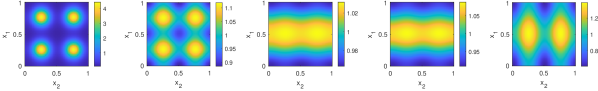
Figure 1: This figure shows the density evolution of $\rho(x,t)$ in the MFG model with congestion parameters $\alpha=1,\beta=2,\epsilon=0.1$ and viscosity $\nu=0.1$, as detailed in Section 4.1. Moving from left to right, at time points $t=0,0.25,0.5,0.75,1$, the density starts in the form of $4$ Gaussians and eventually concentrates at points $(0.5,0.25)$ and $(0.5,0.75)$.

To show that the convergence rate is independent of the grid-size, we set error tolerance $\varepsilon_{1}=10^{-3},\varepsilon_{2}=10^{-4},\varepsilon_{3}=10^{-5}$, and compute the number of iterations the algorithm needs to guarantee that the discretized continuity equation Eq. 38 satisfies

$$\text{Err}^{n}:=\|\text{discretized continuity equation at $n$-th iteration }\|_{L^{2}}<\varepsilon.$$

Here, the norm $\|\cdot\|_{L^{2}}$ has been properly scaled with the spatial and temporal discretization $\Delta h,\Delta t$. We perform computations for various grid-sizes and summarize the results in Fig. 2.

We fixed the optimization step-sizes $\sigma=\tau=0.5$. Although preconditioning increases the computational cost per iteration, it is important to emphasize that it ultimately enhances the computational efficiency. To this end, we consider a scenario without preconditioning with $N_{h}=20$ and $N_{t}=16$, and the algorithm needs $59723$ iterations (taking $508.73$ seconds) to achieve a residual error smaller than $\varepsilon_{1}=10^{-3}$, and $110093$ iterations (taking $932.74$ seconds) to reach a residual error smaller than $\varepsilon_{2}=10^{-4}$. This example highlights how suitable choices of norms and inner products in the PDHG improves the overall efficiency of the proposed algorithm.

$N_{h}$	$N_{t}$	$\varepsilon_{1}=10^{-3}$	$\varepsilon_{2}=10^{-4}$	$\varepsilon_{3}=10^{-5}$
20	16	107 (1.34 s)	137 (1.69 s)	196 (2.37 s)
32	20	117 (4.67 s)	147 (5.83 s)	197 (7.77 s)
40	32	117 (11.19 s)	157 (14.62 s)	197 (18.57 s)

Figure 2: We record the number of iterations our algorithm requires to reach specific error thresholds, $\varepsilon$, across various mesh densities, along with the computational time needed (in seconds). Since the algorithm is not optimized for parallel execution, the computational time increases with the refinement of the mesh.

4.2 Viscosity Effect

In this section, we conduct experiments to demonstrate the impact of the viscosity parameter $\nu$ in the MFG model with congestion. The parameters $\alpha,\beta,\epsilon$ are the same as in the previous section, and we compute the solutions for $\nu=0,0.02,0.1$. The computations demonstrate that $\nu$ significantly affects the solution, as depicted in Fig. 3. A stronger diffusion results in a more widespread solution. More importantly, the algorithm is robust with respect to small values of $\nu$. This phenomenon is explained by the variational nature of the algorithm that can handle singular problems.

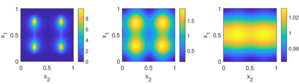
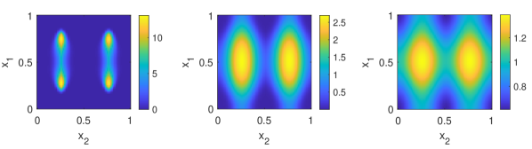
Figure 3: This figure shows the numerical results of density evolution of congestion model with $\nu=0,0.02,0.1$ (from left to right): $\rho(0.5,x)$ (top) and $\rho(1,x)$ (bottom).

4.3 Congestion Effect

In this section, we explore scenarios where $\nu=0$ and the congestion parameter is small $\epsilon$. The goal of these experiments is to study the robustness of the algorithm with respect to further singularity introduced by small values of $\epsilon$. Fig. 4 illustrates that with an increasing congestion coefficient $\epsilon$, the density tends to exhibit reduced movement. Consequently, when $\epsilon=5$, the density undergoes only slight deformation. Additionally, as $\epsilon\rightarrow 0$, the solution consistently demonstrates behavior akin to the leftmost case with $\epsilon=0$. As before, the algorithm demonstrates robust performance in all cases.

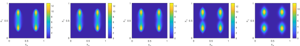
Figure 4: This figure shows the numerical results of density evolution of congestion model with $\epsilon=0,0.02,0.1,1,5$ (from left to right): $\rho(0.5,x)$ (top) and $\rho(1,x)$ (bottom).

References

- [1] Y. Achdou and I. Capuzzo-Dolcetta, Mean field games: numerical methods, SIAM J. Numer. Anal., 48 (2010), pp. 1136–1162, https://doi.org/10.1137/090758477, https://doi.org/10.1137/090758477.
- [2] Y. Achdou and A. Porretta, Mean field games with congestion, Ann. Inst. H. Poincaré C Anal. Non Linéaire, 35 (2018), pp. 443–480, https://doi.org/10.1016/j.anihpc.2017.06.001, https://doi.org/10.1016/j.anihpc.2017.06.001.
- [3] N. Almulla, R. Ferreira, and D. Gomes, Two numerical approaches to stationary mean-field games, Dynamic Games and Applications, 7 (2017), pp. 657–682, https://doi.org/10.1007/s13235-016-0203-5, https://doi.org/10.1007/s13235-016-0203-5.
- [4] J.-P. Aubin and H. Frankowska, Set-valued analysis, vol. 2 of Systems & Control: Foundations & Applications, Birkhäuser Boston, Inc., Boston, MA, 1990.
- [5] J.-D. Benamou and Y. Brenier, A computational fluid mechanics solution to the Monge-Kantorovich mass transfer problem, Numer. Math., 84 (2000), pp. 375–393, https://doi.org/10.1007/s002110050002, https://doi.org/10.1007/s002110050002.
- [6] J.-D. Benamou and G. Carlier, Augmented Lagrangian methods for transport optimization, mean field games and degenerate elliptic equations, J. Optim. Theory Appl., 167 (2015), pp. 1–26, https://doi.org/10.1007/s10957-015-0725-9.
- [7] J.-D. Benamou, G. Carlier, and F. Santambrogio, Variational mean field games, in Active particles. Vol. 1. Advances in theory, models, and applications, Model. Simul. Sci. Eng. Technol., Birkhäuser/Springer, Cham, 2017, pp. 141–171, https://doi.org/10.1007/978-3-319-49996-3_4.
- [8] L. Briceño Arias, D. Kalise, Z. Kobeissi, M. Laurière, A. Mateos González, and F. J. Silva, On the implementation of a primal-dual algorithm for second order time-dependent mean field games with local couplings, in CEMRACS 2017—numerical methods for stochastic models: control, uncertainty quantification, mean-field, vol. 65 of ESAIM Proc. Surveys, EDP Sci., Les Ulis, 2019, pp. 330–348.
- [9] L. M. Briceño Arias, D. Kalise, and F. J. Silva, Proximal methods for stationary mean field games with local couplings, SIAM J. Control Optim., 56 (2018), pp. 801–836, https://doi.org/10.1137/16M1095615, https://doi.org/10.1137/16M1095615.
- [10] F. Camilli and Q. Tang, A convergence rate for the newton’s method for mean field games with non-separable hamiltonians, 2023, https://arxiv.org/abs/2311.05416.
- [11] P. L. Combettes, Perspective functions: properties, constructions, and examples, Set-Valued Var. Anal., 26 (2018), pp. 247–264, https://doi.org/10.1007/s11228-017-0407-x, https://doi.org/10.1007/s11228-017-0407-x.
- [12] D. A. Gomes and J. Saúde, Numerical methods for finite-state mean-field games satisfying a monotonicity condition, Applied Mathematics & Optimization, 83 (2021), pp. 51–82, https://doi.org/10.1007/s00245-018-9510-0, https://doi.org/10.1007/s00245-018-9510-0.
- [13] D. A. Gomes and X. Yang, The hessian riemannian flow and newton’s method for effective hamiltonians and mather measures, ESAIM: M2AN, 54 (2020), pp. 1883–1915, https://doi.org/10.1051/m2an/2020036, https://doi.org/10.1051/m2an/2020036.
- [14] M. Huang, P. E. Caines, and R. P. Malhamé, Large-population cost-coupled LQG problems with nonuniform agents: individual-mass behavior and decentralized -Nash equilibria, IEEE Trans. Automat. Control, 52 (2007), pp. 1560–1571, https://doi.org/10.1109/TAC.2007.904450, https://doi.org/10.1109/TAC.2007.904450.
- [15] M. Huang, R. P. Malhamé, and P. E. Caines, Large population stochastic dynamic games: closed-loop McKean-Vlasov systems and the Nash certainty equivalence principle, Commun. Inf. Syst., 6 (2006), pp. 221–251, http://projecteuclid.org/euclid.cis/1183728987.
- [16] S. Kakutani, A generalization of Brouwer’s fixed point theorem, Duke Math. J., 8 (1941), pp. 457–459, http://projecteuclid.org/euclid.dmj/1077492791.
- [17] J.-M. Lasry and P.-L. Lions, Jeux à champ moyen. I. Le cas stationnaire, C. R. Math. Acad. Sci. Paris, 343 (2006), pp. 619–625, https://doi.org/10.1016/j.crma.2006.09.019, https://doi.org/10.1016/j.crma.2006.09.019.
- [18] J.-M. Lasry and P.-L. Lions, Jeux à champ moyen. II. Horizon fini et contrôle optimal, C. R. Math. Acad. Sci. Paris, 343 (2006), pp. 679–684, https://doi.org/10.1016/j.crma.2006.09.018, https://doi.org/10.1016/j.crma.2006.09.018.
- [19] J.-M. Lasry and P.-L. Lions, Mean field games, Jpn. J. Math., 2 (2007), pp. 229–260, https://doi.org/10.1007/s11537-007-0657-8, https://doi.org/10.1007/s11537-007-0657-8.
- [20] M. Laurière, J. Song, and Q. Tang, Policy iteration method for time-dependent mean field games systems with non-separable hamiltonians, Applied Mathematics & Optimization, 87 (2023), p. 17, https://doi.org/10.1007/s00245-022-09925-5, https://doi.org/10.1007/s00245-022-09925-5.
- [21] S. Liu and L. Nurbekyan, Splitting methods for a class of non-potential mean field games, 2020, https://arxiv.org/abs/2007.00099.
- [22] B. C. Vũ, A splitting algorithm for dual monotone inclusions involving cocoercive operators, Adv. Comput. Math., 38 (2013), pp. 667–681, https://doi.org/10.1007/s10444-011-9254-8, https://doi.org/10.1007/s10444-011-9254-8.