Benchmarking Counterfactual Image Generation

Abstract

Counterfactual image generation is pivotal for understanding the causal relations of variables, with applications in interpretability and generation of unbiased synthetic data. However, evaluating image generation is a long-standing challenge in itself. The need to evaluate counterfactual generation compounds on this challenge, precisely because counterfactuals, by definition, are hypothetical scenarios without observable ground truths. In this paper, we present a novel comprehensive framework aimed at benchmarking counterfactual image generation methods. We incorporate metrics that focus on evaluating diverse aspects of counterfactuals, such as composition, effectiveness, minimality of interventions, and image realism. We assess the performance of three distinct conditional image generation model types, based on the Structural Causal Model paradigm. Our work is accompanied by a user-friendly Python package which allows to further evaluate and benchmark existing and future counterfactual image generation methods. Our framework is extendable to additional SCM and other causal methods, generative models, and datasets.

1 Introduction

“How would I look if I had a beard?", “How a medical scan would be if a patient had disease X?" Counterfactual questions arising from images are very common in science and everyday life. From generating hypothetical visualisations for decision-making to data augmentations for robust model training, counterfactual image generation has emerged as a pivotal domain in the field of artificial intelligence[50, 18].

However, evaluating the efficacy of methods for counterfactual image generation poses a considerable challenge [52]. By definition, counterfactual generation lacks ground truth: e.g., we can’t expect a patient to simultaneously have and not have a disease. This radically complicates the evaluation of counterfactual image generation. Given the importance and frequency with which we move towards counterfactual reasoning in scientific decision-making and everyday life, it is of paramount importance to identify suitable mechanisms for evaluating counterfactual image generation algorithms.

Under a Pearlian methodology of causality, we adopt a set of Structural Causal Models (SCM) [32] to inform generative models about causal relations between factors that affect image generation. Based on the SCM, we employ the counterfactual inference paradigm of Abduction-Action-Prediction and the mechanisms of Deep Structural Causal Models (Deep-SCM) [31] to assess the performance of each method investigated. As such, in this paper, we introduce a comprehensive framework to extensively evaluate any published method on SCM-based counterfactual image generation.

In short, the main contributions of our work are: (1) We develop a comprehensive framework to evaluate the performance of any published image generation method under the Deep-SCM paradigm. While our work focuses on evaluating methods that fall into this category, it can incorporate further/ future causal mechanisms, generative models and datasets. (2) The systematisation of counterfactual image evaluation metrics. (3) We argue in favour of adopting realism and minimality as evaluation metrics for determining successful counterfactuals. (4) The platformisation of the framework in an easy to use python package. (5) The benchmarking and side-by-side comparison of the 3 most prominent families of models used for causal SCM-based counterfactual image generation.

2 Related work

Causal Counterfactual Image Generation: The pairing of SCM s with deep learning mechanisms for counterfactual image generation can be traced back to the introduction of the Deep-SCM framework [31]. The authors utilise normalising flows [44] and variational inference [20] to infer the exogenous noise and perform causal inference under the no unobserved confounding assumption. Follow-up work [4] incorporates hierarchical latent variable models [2] to improve the fidelity of counterfactuals. In parallel, Generative Adversarial Networks (GANs) [11, 7] have been used to perform counterfactual inference through an adversarial objective [3].

GANs have been previously used in [23] to predict reparametrised distributions over image attributes, but only for interventional inference, while Variational Autoencoders (VAEs) have been used for counterfactual inference [51], focusing on learning structured representations from data, and capturing causal relationships between variables, thus diverging from the above scope. Diffusion models [17, 42] were also recently used for this task [37, 36, 9], approaching the noise abduction as a forward diffusion process. However, the aforementioned work only addresses the scenario of a single variable affecting the image.

Similarly to Deep-SCM, normalising flows and VAEs were used in [22], following a backtracking approach [24]. In backtracking interpretation of counterfactuals, causal mechanisms remain unchanged under intervention, but the exogenous noise is modified. Another line of work, [35], utilises deep twin networks [49] to perform counterfactual inference in the latent space instead of Abduction-Action-Prediction paradigm. Since these methods deviate from our scope and focus on Deep-SCM-based causal counterfactuals, we chose not to include them in the current benchmark. As we aim to explore further causal mechanisms, models and data, we believe that these methods are worthwhile future extensions of our current work.

Evaluation of counterfactuals: To the best of our knowledge, there is no previous work in developing a comprehensive framework to extensively evaluate the performance of counterfactual image generating methods, considering the quality of generated images, as well as their relation to factuals and intervened variables. Our work concentrates on addressing this gap in the literature. A study relevant to ours is [45], which compares established methods for counterfactual explainability [27, 5]. However, the main focus lies on creating counterfactual explanations for classifiers which are done only on one dataset (MorphoMNIST), by solely utilising causal generative models [31, 3].

Although there is no systematic comparison across models and data, various metrics have been proposed for counterfactual image generation. For instance, Monteiro et al. [30] introduce metrics, based on the axiomatic definition of counterfactuals [12, 10], namely the properties that arise from the mathematical formulation of SCMs, which we adopt in our work. The authors of [48] evaluate sparsity of counterfactual explanations via elastic net loss and similarity of factual and counterfactual distributions via autoencoder reconstruction errors. Sanchez & Tsaftaris [37] introduce a metric for evaluating minimality through the latents of a VAE, which we adopt in our work.

Optimising over criteria of causal faithfulness (such as the above), does not directly account for quality of produced images. Evaluation metrics that are used in the broader field of image generation include the Fréchet inception distance (FID) [15] and image similarity metrics such as the Learned Perceptual Image Patch Similarity (LPIPS) [53] or CLIPscore [14]. However, these metrics alone do not suffice for the task of image editing; it is common to require spatial information in the form of annotations of expert delineated edit masks information to evaluate a model’s editing abilities [54].

We aspire to explore and include a set of metrics that can consistently evaluate all desired aspects of counterfactual images and serve as proving ground for upcoming methods.

3 Methodology

3.1 Preliminaries

SCM-based counterfactuals The methods we are comparing fall into the common paradigm of SCM-based interventional counterfactuals [19]. A Structural Causal Model (SCM) $\mathcal{G}:=(\mathbf{S},P(\boldsymbol{\epsilon}))$ consists of:

1. A collection of structural assignments, called mechanisms $\mathbf{S}=\{f_{i}\}_{i=1}^{N}$, s.t. $x_{i}=f_{i}(\epsilon_{i},\mathbf{pa}_{i})$; and

2. A joint distribution $P(\boldsymbol{\epsilon})=\prod_{i=1}^{N}p(\epsilon_{i})$ over mutually independent noise variables,

where $x_{i}$ is a random variable, $\mathbf{pa}_{i}$ are the parents of $x_{i}$ (its direct causes) and $\epsilon_{i}$ is a random variable (noise). $x_{i}$ and $\mathbf{pa}_{i}$ are observable variables, hence termed endogenous, while $\epsilon_{i}$ is unobservable, exogenous.

Causal relationships are represented by a causal graph in the form of a directed acyclic graph (DAG). Because of this acyclicity, we can recursively solve for $x_{i}$ and obtain a function $\mathbf{x}=\mathbf{f}(\boldsymbol{\epsilon})$. In our context, we assume $\mathbf{x}$ to be a collection of observable variables, where $x_{i}$ can be a high-dimensional object such as an image and $x_{j\neq i}$ attributes of that image.

The assumptions made in the causal models we examine are: (i) The causal graph is known (captured by a SCM). (ii) There exist no unobserved confounders (causal sufficiency), which makes the noise variables $\boldsymbol{\epsilon}$ mutually independent. (iii) The causal mechanisms are invertible, which means that we can write $\epsilon_{i}=f_{i}^{-1}(x_{i},\mathbf{pa}_{i})$ for $i\in[1,n]$ and therefore $\boldsymbol{\epsilon}=\mathbf{f}^{-1}(\mathbf{x})$.

Because of the causal interpretation of SCMs, we can also compute interventional distributions, namely predict the effect of an intervention to a specific variable, $P(x_{j}|do(x_{i}=y)$. Interventions are formulated by substituting a structural assignment $x_{i}=f_{i}(\epsilon_{i},\mathbf{pa}_{i})$ with $x_{i}=y$. Since interventions operate at the population level, the unobserved noise variables are sampled from the prior $P(\boldsymbol{\epsilon})$. Counterfactual distributions instead refer to a specific observation and can be written as $P(x_{j,x_{i}=y}|\mathbf{x})$. We assume that the structural assignments change, as previously, but the exogenous noise is identical to the one that produced the observation. For this reason, we have to compute the posterior noise $P(\boldsymbol{\epsilon}|\mathbf{x})$.

Counterfactual queries can be formulated as a three-step procedure, known as the Abduction-Action-Prediction paradigm:

1. Abduction: Infer $P(\boldsymbol{\epsilon}|\mathbf{x})$, the state of the world (exogenous noise) that is compatible with the observation $\mathbf{x}$.

2. Action: Replace the structural equations $do(x_{i}=y)$ corresponding to the intervention, resulting in a modified SCM $\widetilde{\mathcal{G}}:=\mathcal{G}_{\mathbf{x};do(x_{i}=y)}=(\widetilde{\mathbf{S}},P(\boldsymbol{\epsilon}|\mathbf{x})$.

3. Prediction: Use the modified model to compute $P_{\widetilde{\mathcal{G}}}(\mathbf{x})$.

Mechanisms In the context of counterfactual image generation, we examine the effect of a change to a parent variable (attribute) on the image. From now on, we will use the notation $x$ and $x^{*}$ for the factual and counterfactual image respectively, and $pa_{x}$, $pa^{*}_{x}$ for the factual and counterfactual attributes.

The conventional linear mechanisms that have been used in the statistical literature for deriving SCMs are not useful when modelling high-dimensional variables, such as images [40]. To overcome this limitation, end-to-end deep learning techniques have been incorporated in the field of causal inference [8]. The framework we are examining, called Deep-SCM [31] is a prime example of such innovation. Introducing invertible mechanisms for all causal variables, enables tractable counterfactual inference by following the aforementioned Abduction-Action-Prediction paradigm.

Three categories of invertible mechanisms are introduced:

1. Invertible, explicit used for the attribute mechanisms in conjunction with Conditional Normalising Flows [46]. This mechanism is invertible by design.

2. Amortised, explicit employed for high-dimensional variables, such as images. This can be developed with Conditional VAE s [20, 16] or extensions like Conditional Hierarchical Variational Autoencoder (HVAE) [21, 41]. The structural assignment is decomposed into a low-level invertible component, in practice the reparametrisation trick, and a high-level non-invertible component that is trained in an amortized variational inference manner, which in practice can be a probabilistic convolutional decoder. This also entails a noise decomposition of $\epsilon_{i}$ into two noise variables $(\epsilon,z)$, s.t. $P(\epsilon_{i})=P(\epsilon)P(z)$.

3. Amortised, implicit This mechanism can also be employed for the imaging variables. However, it does not rely on approximate maximum-likelihood estimation for training, but optimises an adversarial objective with a conditional implicit-likelihood model. It was introduced in [3] and developed further with Conditional GANs [28, 7].

3.2 Methods Considered in the Benchmark

Conditional Normalising Flows To enable tractable abduction of $pa_{x}$, invertible mechanisms can be learned using conditional normalising flows. A normalising flow maps between probability densities defined by a differentiable, monotonic, bijection. These mappings are a series of relatively simple invertible transformations and can be used to model complex distributions [44]. The mechanism for each attribute ($pa_{x}$) is a normalising flow $f(\epsilon)$. The base distribution for the exogenous noise is typically assumed to be Gaussian $\epsilon\sim N(0,I)$. The distribution of $pa_{x}$ can be computed as $P(pa_{x})=P(\epsilon)\left|\text{det}\,\nabla f(\epsilon)\right|^{-1}$. Thus, the conditional distribution $P(pa_{x}|pa_{pa_{x}})$ can be computed as:

$$P(pa_{x}|pa_{pa_{x}})=p(\epsilon)\left|\text{det}\,\nabla f(\epsilon;pa_{pa_{x}})\right|^{-1}$$ (1)

Conditional VAE To produce counterfactuals via leveraging conditional VAE s [20, 16], the high-dimensional variable $x$ along with its factual parents $pa_{x}$ are encoded into a latent representation $z\sim q_{\phi}(z|x,pa_{x})$ which is sampled through the reparameterisation trick: $z=\mu_{\phi}(x,pa_{x})+\sigma_{\phi}(x,pa_{x})*\epsilon$, where $\epsilon\sim N(0,I)$ [4]. Then, the latent variable $z$ and the counterfactual parents $pa^{*}_{x}$ are decoded to obtain the counterfactual distribution $(\mu_{\theta}^{*},\sigma_{\theta}^{*})$. Since the observational distribution is assumed to be Gaussian, sampling can be performed by forwarding the decoder with the factual parents and then applying a reparametrization: $x=\mu_{\theta}(z,pa_{x})+\sigma_{\theta}(z,pa_{x})*\epsilon$, $\epsilon\sim N(0,I)$. Thus, the exogenous noise can be expressed as $\epsilon=\frac{x-\mu_{\theta}(z,pa_{x})}{\sigma_{\theta}(z,pa_{x})}$. Finally, this $\epsilon$ is used to sample from the counterfactual distribution as follows: $x^{*}=\mu_{\theta}(z,pa^{*}_{x})+\sigma_{\theta}(z,pa^{*}_{x})*\epsilon$.

Conditional HVAE A conditional structure of the top-down HVAE [41, 2, 47] can be adopted to improve the quality of produced samples and abduct noise more accurately. As we consider Markovian SCMs, the exogenous noise $\boldsymbol{\epsilon}$ has to be independent, therefore as the latents $z_{1:L}$ are downstream components of the exogenous noise, the corresponding prior $p_{\theta}(z_{1:L})$ has to be independent from $pa_{x}$. In order to accomplish this, the authors of [4] propose to incorporate $z_{i}$ and $pa_{x}$ at each top-down layer through a function $f^{i}_{\omega}$ which is modelled as a learnable projection network. Particularly, the output of each top-down layer can be written as:

$$h_{i}=h_{i+1}+f^{i}_{\omega}(z_{i},pa_{x}),\hskip 14.22636ptz_{i}\sim p_{\theta}(z_{i}|z_{>i}),\hskip 14.22636pti=L-1,...,1,$$ (2)

where $h_{init}$ can be learned from data. Thus, the joint distribution of $x,z_{1:L}$ conditioned on $pa_{x}$ can be expressed as:

$$p_{\theta}(x,z_{1:L}|pa_{x})=p_{\theta}(x|z_{1:L},pa_{x})p_{\theta}(z_{1:L}),$$ (3)

while the conditional approximate posterior is defined as:

$$q_{\phi}(z_{1:L}|x,pa_{x})=q_{\phi}(z_{L}|x,pa_{x})q_{\phi}(z_{L-1}|z_{L},x,pa_{x})...q_{\phi}(z_{1}|z_{i>1},x,pa_{x})$$ (4)

Following a methodology analogous to standard VAE, the exogenous noise can be abducted as $\epsilon=\frac{x-\mu_{\theta}(z_{1:L},pa_{x})}{\sigma_{\theta}(z_{1:L},pa_{x})}$. Therefore, a counterfactual sample can be obtained as: $x^{*}=\mu_{\theta}(z_{1:L},pa^{*}_{x})+\sigma_{\theta}(z_{1:L},pa^{*}_{x})*\epsilon$.

Conditional GAN Finally, we also consider the conditional GAN-based framework [3] for counterfactual inference. This setup includes an encoder $E$, that given an image $x$ and its parent variables $pa_{x}$ produces a latent code $z_{x}=E(x,pa_{x})$. The generator $G$ then receives either a noise latent $z$ or the produced $z_{x}$ together with the parents $pa_{x}$ to produce an image $x^{\prime}=G(z^{\prime},pa_{x})$. The image alongside the latent and the parents $pa_{x}$ are then fed into the discriminator. The encoder and the generator are trained together as in [7] to deceive the discriminator in classifying generated samples from a noise latent $z$ as real, while classifying samples produced from $z_{x}$ (real image latents) as fake, while the discriminator has the opposite objective. Providing $pa_{x}$ as input to all models is proven to make conditioning on parents stronger. The conditional GAN is optimised as follows:

$$\min_{E,G}\max_{D}V(D,G,E)=\mathbb{E}_{q(x)p(pa_{x})}[log(D(x,E(x,pa_{x}),pa_{x}))]$$ (5)

$$+\mathbb{E}_{p(z)p(pa_{x})}[log(1-D(G(z,pa_{x}),z,pa_{x}))],$$

where $q(x)$ is the distribution for the images, $p(z)\sim N(0,I)$ and $p(pa_{x})$ is the distribution of the parents. To produce counterfactuals images, the factual $x$ and its parents $pa_{x}$ are given to the encoder which produces the latent $z_{x}$ which serves as the noise variable. Then, the counterfactual parents $pa^{*}_{x}$ and $z_{x}$ are fed into the generator to produce the counterfactual image $x^{*}$. This procedure can be formulated as:

$$x^{*}=G(E(x,(pa_{x})),pa^{*}_{x}),$$ (6)

However, as it is discussed in the original paper [3] and as we confirmed empirically, this objective is not enough to enforce accurate abduction of the noise, resulting in low reconstruction quality. In order to alleviate this, the encoder is fine-tuned, while keeping the rest of the network fixed, to minimise explicitly the reconstruction loss on image and latent space. This cyclic cost minimisation approach, introduced by [6], enables accurate learning of the inverse function of the generator.

3.3 Evaluation Metrics

The evaluation of counterfactual inference has been formalised through the axioms of [10, 12]. The authors of [30] utilise such an axiomatic definition to introduce three metrics for evaluating image counterfactuals: Composition, Effectiveness, and Reversibility . While it is necessary for counterfactual images to respect these axiom-based metrics, we find that they are not sufficient for a perceptual definition of successful counterfactuals. The additional desiderata we consider are realism of produced images, as well the minimality or sparseness of changes. For the former, we employ the FID metric, whilst for the latter, we employ the Counterfactual Latent Divergence metric proposed in [37]. All adopted metrics do not require access to ground truth counterfactuals.

Composition If we force a variable $X$ to a value $x$ it would have without the intervention, it should have no effect on the other variables [10]. It follows then, that we can have a null-intervention that should leave all variables unchanged. Based on this property one can apply the null-intervention $m$ times, denoted as $f^{m}_{\emptyset}$, and measure the $l_{1}$ distance $d(\cdot)$ between the $m$ produced and the original image [30]. To produce a counterfactual under the null-intervention, we abduct the exogenous noise and skip the action step.

$$\text{composition}^{m}(x,pa_{x})=d(x,f^{m}_{\emptyset}(x,pa_{x}))$$ (7)

As the $\ell_{1}$ distance on image space yields results that do not align with our perception and favours shortcut features such as simpler backgrounds, we extend Composition by computing the $\ell_{1}$ norm of VGG-16 embeddings and the Learned Perceptual Similarity (LPIPS) [53].

Effectiveness aims to identify how successful is the performed intervention. In other words, if we force a variable $X$ to have the value $x$, then $X$ will take on the value $x$ [10]. In order to quantitatively evaluate effectiveness for a given counterfactual image we leverage an anti-causal predictor $g^{i}_{\theta}$ trained on the data distribution, for each parent variable $pa^{i}_{x}$  [30]. Each predictor, then, approximates the counterfactual parent $pa^{i*}_{x}$ given the counterfactual image $x^{*}$ as input

$$\text{effectiveness}_{i}(x^{*},pa^{i*}_{x})=d(pa^{i*}_{x},g^{i}_{\theta}(x^{*})),$$ (8)

where $d(\cdot)$ is the corresponding distance, defined as a classification metric for categorical variables and as a regression metric for continuous ones.

Realism For realism we use the Fréchet Inception Distance (FID) [15] which captures the similarity of the set of counterfactual images to all images in the dataset. Real and counterfactual samples are fed into an Inception v3 model [43] trained on ImageNet, in order to extract their feature representations, that capture high-level semantic information.

Minimality The need for minimality of counterfactuals can be justified on the basis of the sparse mechanism shift hypothesis [39]. While we can achieve an approximate estimate of minimality by combining the composition and effectiveness metrics, we find that an additional metric is helpful to measure the closeness of the counterfactual image to the factual. For this reason, we leverage a modified version of the Counterfactual Latent Divergence (CLD) metric introduced in [37]:

$$\text{CLD}=\log(w_{1}\exp{P(S_{x^{*}}\leq div)}+w_{2}\exp{P(S_{x}\geq div)}),$$ (9)

where $div$ is the distance of the counterfactuals $x^{*}$ from the factuals $x$, $S_{x}$, $S_{x^{*}}$ are the sets of all distances of the factual image to the images that have the same label as the factual and the counterfactual, respectively: $S_{x}=\{d(x,x^{\prime})|pa_{x^{\prime}}=pa_{x}\}$, $S_{x^{*}}=\{d(x,x^{\prime})|pa_{x^{\prime}}=pa_{x^{*}}\}$, where $x^{\prime}$ is any image from the data distribution and $pa_{x^{\prime}}$ is the variable being intervened upon. To compute the distance $d(\cdot)$, we train an unconditional VAE and use the KL divergence between the latent distributions: $d(x_{i},x_{j})=D_{KL}(\mathcal{N}(\mu_{i},\sigma_{i}),\mathcal{N}(\mu_{j},\sigma_{j})$. This metric is minimised by keeping both probabilities low, which represent a trade-off between being far from the factual class but not as far as other (real) images from the counterfactual class are. The weights $w_{1}$, $w_{2}$ depend on the effective difference each variable has on the image.

(a) MorphoMNIST
t: thickness, i: intensity, d: digit, im: image

(b) CelebA
s: smiling, e: eyeglasses, im: image

Figure 1: Causal graphs for our datasets, MorphoMNIST and CelebA.

4 Results

Datasets Given the availability of results and architectures from literature, we benchmark all the above models on MorphoMNIST (32x32) [1] and CelebA (64x64) [26]. We assume the causal graphs of Figure 1 (a) for MorphoMNIST and (b) for CelebA. MorphoMNIST is a purely synthetic dataset generated by inducing morphological operations on the well-established MNIST digits. We note, that interventions on thickness affect both the intensity and image (Figure 1(a)). Therefore, we should be able to measure this effect on intensity by comparing the prediction of the normalising flow for this variable with the prediction of the regressor for the produced image. Meanwhile, CelebA is based on real world images, and hence we use two assumed disentangled attributes as done in [30] Figure 1(b). No additional layer of parents is involved. These attributes are independent to each other which satisfies the criterion for counterfactual inference.

Setup For Normalising Flows we leverage the normflows package [44], using the QuadraticSpline, ConstScaleShift and conditional ScaleShift flow layers of [22]. For the MorphoMNIST dataset, we compare the VAE architecture as given in the original Deep-SCM paper [31], the HVAE architecture of [4] and the fine-tuned GAN architecture of [45] as the set up of [3] failed to converge. For CelebA, we use the VAE architecture proposed as baseline in [3], while we extend the HVAE used in [30] with the conditioning mechanisms of [4]. Finally, for the GAN we used the architecture proposed in [3].

We compare VAE with a fixed standard deviation of $\sqrt{e^{-5}}$ as used in [31, 3] versus a VAE with learnable standard deviation. For MorphoMNIST we trained the HVAE as described in 3.2 and used the counterfactual training for CelebA as we found it to ignore conditioning, detailed in 4.2. We experimented with different values for $\beta$ and found that $\beta=1$ and $\beta=5$ perform better for MorphoMNIST and CelebA, respectively. For GAN, we found that fine-tuning the cyclic cost minimisation was necessary to ensure closeness to the factual image for both datasets.

Table 1: Composition for MorphoMNIST. For embeddings, we concatenate the last layer activations across all predictors trained.

	$l_{1}$ image space $\downarrow$		$l_{1}$ embeddings $\downarrow$		LPIPS $\downarrow$
Model	1 cycle	10 cycles	1 cycle	10 cycles	1 cycle	10 cycles
VAE ($\sigma=\sqrt{e^{-5}}$)	$4.244_{2.158}$	$9.855_{4.768}$	$0.095_{0.042}$	$0.158_{0.064}$	$0.039_{0.003}$	$0.098_{0.003}$
VAE ($\sigma$ learned)	$2.600_{1.454}$	$7.698_{4.199}$	$0.064_{0.033}$	$0.135_{0.057}$	$0.026_{0.003}$	$0.075_{0.003}$
HVAE	$\mathbf{0.438_{0.178}}$	$\mathbf{1.550_{0.541}}$	$\mathbf{0.009_{0.004}}$	$\mathbf{0.038_{0.015}}$	$\mathbf{0.006_{0.001}}$	$\mathbf{0.024_{0.003}}$
GAN	$16.779_{8.406}$	$16.780_{8.401}$	$0.193_{0.065}$	$0.193_{0.065}$	$0.154_{0.004}$	$0.154_{0.004}$
GAN fine-tuned	$3.807_{1.822}$	$11.697_{5.750}$	$0.089_{0.042}$	$0.272_{0.106}$	$0.049_{0.004}$	$0.184_{0.008}$

4.1 Composition

To quantitatively evaluate composition, we perform a null intervention. Following the protocol of [30], we apply composition for one and for ten cycles, measuring the distance between the initial observable image and its first and tenth reconstructed versions respectively. In addition to the $\ell_{1}$ distance in the pixel space, we also use the LPIPS [53] metric and the $\ell_{1}$ in embedding space.

(a) VAE

(b) HVAE

(c) GAN fine-tuned

Figure 2: Composition for 10 cycles on the MorphoMNIST test set.

MorphoMNIST: In Table 1 we show quantitative results for composition. We extract embeddings by concatenating the last layers of the anticausal predictors and calculate LPIPS on VGG. We can observe that HVAE significantly outperforms all models across metrics both for $composition^{1}$ and $composition^{10}$, while GAN without cyclic cost minimisation performs poorly even from the first cycle. Figure 2 depicts qualitative results for the 10-cycle composition. It is evident that the HVAE is capable of preserving extremely well the details of the original image; the VAE performs adequately; whereas the GAN introduces the largest distortion after multiple cycles.

Table 2: Composition for CelebA. For the embeddings we use the last layer activation of a pretrained VGG-16 network.

	$l_{1}$ image space $\downarrow$		$l_{1}$ embeddings $\downarrow$		LPIPS $\downarrow$
Model	1 cycle	10 cycles	1 cycle	10 cycles	1 cycle	10 cycles
VAE ($\sigma=\sqrt{e^{-5}}$)	$126.8_{19.3}$	$126.4_{22.1}$	$0.536_{0.100}$	$0.553_{0.099}$	$0.332_{0.004}$	$0.462_{0.004}$
VAE ($\sigma$ learned)	$127.8_{18.1}$	$\mathbf{123.4_{22.1}}$	$0.527_{0.102}$	$0.549_{0.102}$	$0.295_{0.004}$	$0.424_{0.005}$
HVAE fine-tuned	$129.4_{11.6}$	$138.8_{23.4}$	$\mathbf{0.498_{0.121}}$	$\mathbf{0.525_{0.121}}$	$\mathbf{0.063_{0.003}}$	$\mathbf{0.200_{0.008}}$
GAN	$118.9_{21.1}$	$126.1_{17.1}$	$0.548_{0.121}$	$0.660_{0.132}$	$0.403_{0.004}$	$0.506_{0.004}$
GAN fine-tuned	$\mathbf{115.3_{22.0}}$	$128.4_{21.4}$	$0.516_{0.120}$	$0.592_{0.133}$	$0.290_{0.003}$	$0.462_{0.005}$

CelebA: We confirm empirically that computing distances on pixel space for a dataset that contains complex real world images is not informative and therefore we resort to pretrained VGG-16 embeddings and LPIPS to effectively capture meaningful differences. From Table 2 we observe that HVAE achieves the best composition scores in terms of $l^{(1)}$ embeddings and LPIPS distance, while GAN again performs the worst. We can further verify the efficacy of HVAE from the qualitative results of Figure 3. Particularly, it retains the details of the original image, while VAE progressively blurs and distorts it during repeating cycles. GAN with cyclic cost minimisation does not introduce blurriness, but alters significantly both the image style and content.

(a) VAE ($\sigma$ learned)

(b) HVAE

(c) GAN fine-tuned

Figure 3: Composition for 10 cycles on CelebA test set.

4.2 Effectiveness

MorphoMNIST: To quantitatively evaluate effectiveness on MorphoMNIST, we train convolutional regressors for continuous variables (thickness, intensity) and a classifier for categorical variables (digits). We perform random interventions on a single parent each time, as per [4]. In Table 3, we can observe that the mechanism of HVAE achieves the best performance in the majority of the interventional scenarios.

Table 3: Effectiveness on MorphoMNIST test set.

	Thickness (t) MAE $\downarrow$			Intensity (i) MAE $\downarrow$			Digit (y) Acc. $\uparrow$
Model	$do(t)$	$do(i)$	$do(y)$	$do(t)$	$do(i)$	$do(y)$	$do(t)$	$do(i)$	$do(y)$
VAE ($\sigma=\sqrt{e^{-5}}$)	$0.125_{0.01}$	$0.346_{0.01}$	$0.138_{0.01}$	$9.382_{0.57}$	$20.642_{0.59}$	$11.279_{0.56}$	$0.988_{0.01}$	$\mathbf{0.989_{0.01}}$	$0.933_{0.02}$
VAE ($\sigma$ learned)	$0.109_{0.01}$	$0.333_{0.02}$	$0.139_{0.01}$	$3.149_{0.26}$	$5.326_{0.29}$	$4.64_{0.35}$	$\mathbf{0.989_{0.01}}$	$0.988_{0.01}$	$0.775_{0.02}$
HVAE	$\mathbf{0.086_{0.09}}$	$\mathbf{0.224_{0.03}}$	$\mathbf{0.117_{0.01}}$	$\mathbf{1.991_{0.18}}$	$\mathbf{3.517_{0.26}}$	$\mathbf{2.098_{0.17}}$	$0.985_{0.01}$	$0.935_{0.02}$	$\mathbf{0.972_{0.02}}$
GAN	$0.227_{0.01}$	$0.631_{0.02}$	$0.214_{0.01}$	$6.680_{0.25}$	$9.795_{0.25}$	$6.632_{0.16}$	$0.810_{0.01}$	$0.811_{0.01}$	$0.813_{0.02}$
GAN fine-tuned	$0.228_{0.01}$	$0.680_{0.02}$	$0.393_{0.02}$	$9.436_{0.59}$	$15.137_{0.99}$	$12.388_{0.57}$	$0.961_{0.02}$	$0.966_{0.01}$	$0.451_{0.024}$

We note that the error for intensity remains low when performing an intervention on thickness, compared to other interventions, which showcases the effectiveness of the conditional intensity mechanism. The compliance with the causal graph of Figure 1 can also be confirmed qualitatively in Figure 4. Intervening on thickness modifies intensity, while intervening on intensity does not affect thickness (graph mutilation). Interventions on the digit alter neither.

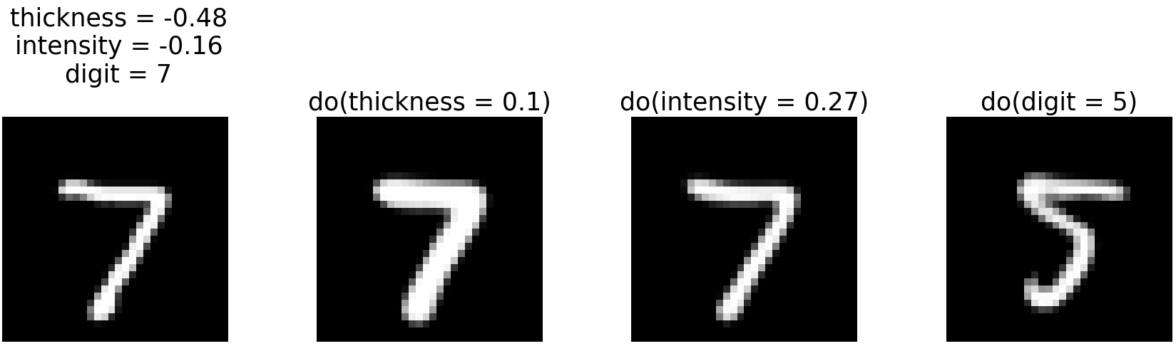
(a) VAE ($\sigma$ learned)

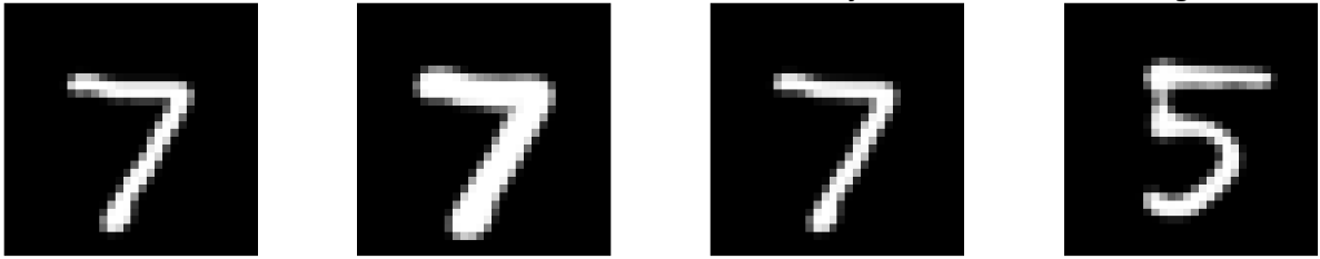
(b) HVAE

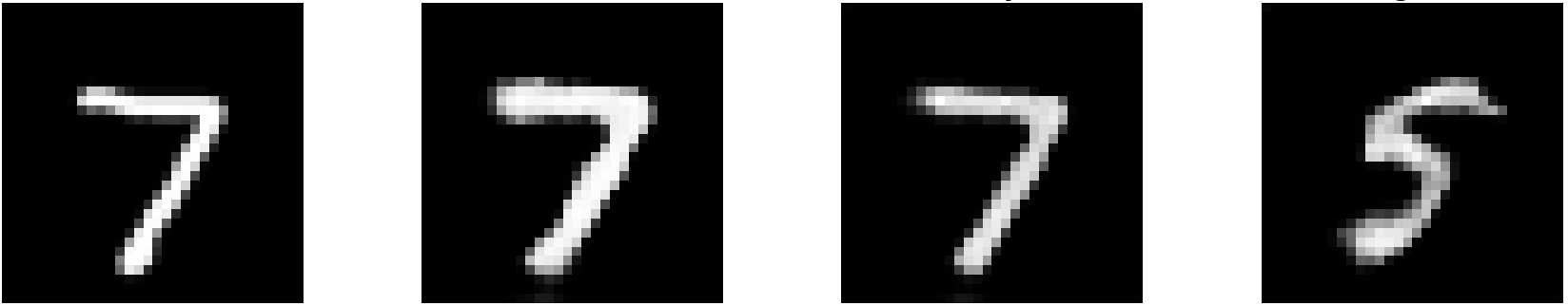
(c) GAN fine-tuned

Figure 4: From left to right: Factual, $do(thickness)$, $do(intensity)$, $do(digit)$

CelebA: To measure counterfactual effectiveness for CelebA, we train binary classifiers for the smiling and eyeglasses attributes. We observe that by training HVAE only with the standard ELBO loss, the model exclusively reconstructs the initial image and systematically ignores the causal/counterfactual condition. To alleviate this, we exploit the counterfactual training process that is proposed in [4]. In brief, the lowest ELBO loss is incorporated early during training into the counterfactual loss by introducing a Lagrange coefficient, thus transforming the setup into a Lagrangian optimisation problem [33].

Table 4 presents the measured effectiveness in terms of F1 score using the attribute classifiers. Reasonable F1 values indicate that all models are capable of performing counterfactual predictions. The fine-tuned HVAE outperforms all other models across most scenarios with the most evident difference being observed in interventions on the attribute eyeglasses. This suggests that HVAE can efficiently manipulate this attribute and generate plausible counterfactuals. On the other hand, we notice that when we intervene on the attribute smiling, the fine-tuned GAN outperforms other models, which indicates that, even if it cannot perform accurate interventions, it can better disentangle this intervention from the attribute eyeglasses.

The following standard data augmentations were applied to mitigate biases existing in the CelebA dataset, which were exploited by the classifiers during training: random flipping, random cropping and colour distortions. Additionally, as CelebA is a highly unbalanced dataset, a weighted sampler is used to ensure a balanced class distribution in each training batch. Arguably, effectiveness is challenging to quantify, since the data-dependent methods that are typically used may lead to biased measurements.

Table 4: Effectiveness on CelebA test set.

	Smiling (s) F1. $\uparrow$		Eyeglasses (e) F1. $\uparrow$
Model	$do(s)$	$do(e)$	$do(s)$	$do(e)$
VAE ($\sigma=\sqrt{e^{-5}}$)	$0.981_{0.01}$	$0.996_{0.01}$	$0.929_{0.05}$	$0.771_{0.02}$
VAE ($\sigma$ learned)	$0.897_{0.02}$	$0.987_{0.01}$	$0.938_{0.05}$	$0.810_{0.02}$
HVAE fine-tuned	$\mathbf{0.998_{0.01}}$	$\mathbf{0.997_{0.01}}$	$0.883_{0.06}$	$\mathbf{0.981_{0.02}}$
GAN	$0.818_{0.02}$	$0.837_{0.02}$	$0.824_{0.04}$	$0.873_{0.01}$
GAN fine-tuned	$0.819_{0.02}$	$0.873_{0.01}$	$\mathbf{0.957_{0.03}}$	$0.891_{0.01}$

In Figure 5 we observe the apparent weakness of VAEs to perform on more complex, real-world images, since its single latent variable can capture only few details from the original images, introducing bluriness. Due to the expressivity of the hierarchical latents, the fine-tuned HVAE is able to retain much of the information of the original image and effectively modify it by following the counterfactual condition. The fine-tuned GAN is also capable of producing counterfactuals that are similar to the factual and adhere to the condition, but of lower quality compared to the HVAE.

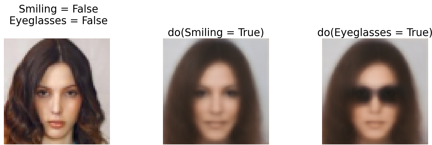
(a) VAE ($\sigma$ learned)

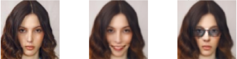
(b) HVAE fine-tuned

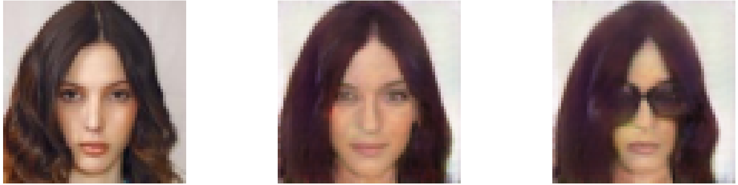
(c) GAN fine-tuned

Figure 5: From left to right: Factual, $do(Smiling)$, $do(Eyeglasses)$

4.3 Realism & Minimality

The FID metric in Table 5 aligns with our qualitative results, showing that HVAE outperforms VAEs on MorphoMNIST and GANs on CelebA. HVAE without counterfactual training performs better on CelebA, as expected, since it does not introduce any information.

For minimality, we report the weighted CLD metric and its component probabilities (Table 5). We report lower values for VAEs on MorphoMNIST, as shown both in CLD and $P(S_{x^{*}}\leq div)$, with HVAE following. In CelebA, HVAEs outperform both VAEs and fine-tuned GAN, whose scores are comparable. We notice that for CelebA, the term $P(S_{x}\geq div)$ cannot effectively discern changes that are too minimal from effective ones, which can be explained by the fact that the intervened variables are not as distinctive as others such as gender or background, making the factual-counterfactual distance essentially too small. This is the motivation for the weighting terms on CLD, which for these experiments are $w_{1}=0.8$, $w_{2}=0.2$. We trained unconditional VAEs for both datasets and found the metric performing similarly even when using distance between different types of embeddings, such as VGG-16 or CLIP [34].

Table 5: Realism and Minimality for MorphoMNIST and CelebA. In the minimality columns, the numbers from left to right are the values for: (i) weighted CLD, (ii) $P(S_{x^{*}}\leq div)$, (iii) $P(S_{x}\geq div)$.

	MorphoMNIST				CelebA
Model	FID $\downarrow$	Minimality $\downarrow$			FID $\downarrow$	Minimality $\downarrow$
VAE ($\sigma=\sqrt{e^{-5}}$)	$17.096$	$0.276$	$0.065$	$0.843$	$77.307$	$0.310$	$0.072$	$0.925$
VAE ($\sigma$ learned)	$10.124$	$\mathbf{0.268}$	$0.055$	$0.839$	$66.412$	$0.297$	$0.014$	$0.984$
HVAE	$\mathbf{5.362}$	$0.272$	$0.112$	$0.736$	$\mathbf{12.667}$	$0.295$	$0.0001$	$0.999$
HVAE fine-tuned	-	-			$22.047$	$\mathbf{0.295}$	$0.003$	$0.996$
GAN	$72.766$	$0.390$	$0.339$	$0.570$	$41.536$	$0.362$	$0.224$	$0.777$
GAN fine-tuned	$35.568$	$0.286$	$0.119$	$0.764$	$31.560$	$0.304$	$0.046$	$0.953$

5 Discussion and Conclusions

Many methods have been introduced for counterfactual image generation. However, to date, a systematic way to assess current and potentially upcoming methods under a single comprehensive framework is missing. Given the rapidly emerging interest in causal representation learning and counterfactual generation, it is of paramount importance to build a unified framework to evaluate and cross-compare different approaches. Our aspiration is therefore to help as well as to inspire further work in the community on this direction. We evaluated three different setups for image mechanisms on four different evaluation metrics. We identify that the development of Deep-SCM-based conditional HVAE is in the right direction, as it outperformed all other models examined (VAEs, GANs) across all metrics performed. Our findings indicate that the hierarchical structure of the latents allows for more expressivity and accurate abduction of the noise variable, versus VAEs and GANs. Moreover, we created a user-friendly framework for follow-up work by future modellers, adaptable to a diverse set of causal methods and assessment metrics for the community to build on and expand further.

Limitations and future work: We examined three families of generative models and two datasets, under the Deep-SCM paradigm. Therefore, we purposely left methods that differ from this paradigm for future work, such as deep twin networks and backtracking counterfactuals. As future work, we also believe that it is important to investigate diffusion models (DM) which have showcased impressive performance on image generation. DM have not been conditioned yet with SCM graphs and we seek to explore this bold direction. An important consideration for DM is that abduction of noise is not always straightforward and thus, conditioning must methodically be considered. We also aim to explore the effect of more complex Deep-SCM structures on the models presented. Applying the proposed framework to further models, datasets and causal mechanisms will shed light on the distinct abilities of conditional generative models. It will also help the community to better understand how generative models interact with causal mechanisms to disentangle confounding attributes and conform to causal paths that determine image generation.

Appendix

In Appendix 0.A we provide more details regarding the model architectures and hyperparameters for all the experiments we ran. In Appendix 0.B we include extra qualitative results for all the models we compare.

Appendix 0.A Experimental details

In the following tables that depict the architectures for our models, F refers to number of filters, K refers to kernel width and height, S refers to stride, P refers to padding, Up refers to the scale of upsampling, BN refers to batch normalization, D refers to dropout probability and A refers to activation function.

0.A.1 Normalising Flows

For Normalising Flows we leverage the normflows package [44] and base our implementation in [22]. While flows can be trained for all attribute variables, in practice we only employ them for the intensity variable, as we discussed in the main paper. In Table 6 we present the architecture for this flow, which is conditioned on its parent variable, thickness. For training the model we use the Adam optimizer with learning rate $10^{-3}$, batch size of 64 and early stopping with the patience parameter set to 2.

Table 6: Normalising Flow Architecture for intensity (MorphoMNIST).

Layers
Masked Affine Autoregressive Flow
Autoregressive Rational Quadratic Spline Flow
Autoregressive Rational Quadratic Spline Flow
Autoregressive Rational Quadratic Spline Flow
Sigmoid Transformation Flow
Constant AddScale Flow
Affine Coupling Flow

0.A.2 VAE

We adopt the VAE implementation as defined in [31, 4]. The output of the VAE decoder is passed though a Gaussian network that is implemented as a convolutional layer to obtain the corresponding $\mu$, $\sigma$. Then, the reconstructed image is sampled with the reparameterisation trick. To condition the model we concatenate the parent variables with the output features of the first Linear layer of the encoder (Tables 7 and 9).

0.A.2.1 MorphoMNIST

The architectures of the VAE encoder and decoder are displayed in Tables 7 and 8, respectively. We train the model until convergence (around 1M iterations) with batch size 256 using the AdamW optimizer with initial learning rate $10^{-3}$, $\beta_{1}$=0.9, $\beta_{2}$=0.9 and weight decay 0.01. Furthermore, we use early stopping with the patience parameter set to 10 and a linear warmup scheduler for the first 100 iterations. The dimension of the latent variable is set to 16. We also apply gradient clipping with value 350 and gradient skipping with value 500.

Table 7: VAE Encoder Architecture for MorphoMNIST.

Layer	F	K	S	P	BN	A
Conv2D	32	5	2	1	N	ReLU
Conv2D	32	3	2	1	N	ReLU
Conv2D	32	3	2	1	N	ReLU
Linear	128	-	-	-	N	ReLU
Linear	128	-	-	-	N	ReLU
Linear (latent dim)	16	-	-	-	N	ReLU

Table 8: VAE Decoder Architecture for MorphoMNIST.

Layer	F	K	S	Up	P	BN	A
Linear	128	-	-	-	-	N	ReLU
Linear	512	-	-	-	-	N	ReLU
Upsample	-	-	-	2x	-	-	-
Conv2D	32	3	1	-	1	N	ReLU
Upsample	-	-	-	2x	-	-	-
Conv2D	32	3	1	-	1	N	ReLU
Upsample	-	-	-	2x	-	-	-
Conv2D	16	5	1	-	2	N	ReLU

0.A.2.2 CelebA

We extend the VAE implementation of [31, 4] to be compatible with higher resolution images (Tables 9 and 10). We train the model until convergence (around 600K iterations) with a batch size of 128 leveraging the Adam optimizer with initial learning rate $5\cdot 10^{-4}$ and $\beta_{1}$=0.9, $\beta_{2}$=0.999. We also use a linear warmup scheduler for the first 100 iterations. Additionally, we set the early stopping patience to 10 and add gradient clipping and gradient skipping with values 350 and 500 respectively. The dimension of the latent variable is set to 16.

Table 9: VAE Encoder Architecture for CelebA.

Layer	F	K	S	P	D	A
Conv2D	32	3	2	1	0.25	LReLU(0.01)
Conv2D	64	3	2	1	0.25	LReLU(0.01)
Conv2D	128	3	2	1	0.25	LReLU(0.01)
Conv2D	256	3	2	1	0.25	LReLU(0.01)
Conv2D	256	1	1	0	-	LReLU(0.01)
Linear	256	-	-	-	-	LReLU(0.01)
Linear	256	-	-	-	-	LReLU(0.01)
Linear (latent dim)	16	-	-	-	-	LReLU(0.01)

Table 10: VAE Decoder Architecture for CelebA.

Linear	F	K	S	Up	P	BN	D	A
Linear	256	-	-	-	-	N	-	ReLU
Linear	4096	-	-	-	-	N	-	-
Upsample	-	-	-	2x	-	-	-	-
Conv2D	256	3	1	-	1	Y	0.25	LReLU(0.01)
Upsample	-	-	-	2x	-	-	-	-
Conv2D	128	3	1	-	1	Y	0.25	LReLU(0.01)
Upsample	-	-	-	2x	-	-	-	-
Conv2D	64	3	1	-	1	Y	0.25	LReLU(0.01)
Upsample	-	-	-	2x	-	-	-	-
Conv2D	32	3	1	-	1	Y	0.25	LReLU(0.01)
Upsample	-	-	-	1x	-	-	-	-
Conv2D	16	3	1	-	1	Y	-	Sigmoid

0.A.3 HVAE

We follow the experimental setup of [4] leveraging the proposed conditional structure of the very deep VAE [2]. To condition the model we expand the parents and concatenate them with the corresponding latent variable at each top-down layer.

0.A.3.1 MorphoMNIST

: We use a group of 20 latent variables with spatial resolutions $\{1,4,8,16,32\}$. Each resolution includes 4 stochastic blocks. The channels of the feature maps per resolution are $\{256,128,64,32,16\}$, while the dimension of the latent variable channels is 16.

We train the model until convergence (approximately 1M iterations) with a batch size of 256 and apply early stopping with patience 10. The resolution of the input images is 32x32. We use the AdamW optimizer with initial learning rate $10^{-3}$, $\beta_{1}$ = 0.9, $\beta_{2}$ = 0.9, a weight decay of 0.01 and a linear warmup scheduler for the first 100 iterations. We additionally add gradient clipping and gradient skipping with values 350 and 500 respectively.

0.A.3.2 CelebA

For the CelebA experiments we slightly extend the architecture in order to be functional with 64x64 images. Particularly, the spatial resolutions are set to $\{1,4,8,16,32,64\}$, while the widths per resolution are $\{1024,512,256,128,64,32\}$. We consider 4 stochastic blocks per resolution leading to a total of 24 latent variables. Finally, we also set the channels of the latent variables to 16.

As we have discussed in the main paper we employ a two phase training which consists of a pretraining stage and a counterfactual fine-tuning stage. We pretrain the model for 2M iterations with a batch size of 32 using the AdamW optimizer with initial learning rate $10^{-3}$, $\beta_{1}$=0.9, $\beta_{2}$=0.9, weight decay 0.01, and early stopping patience set to 10. We use a linear warmup scheduler for the first 100 iterations and also set values for gradient clipping and gradient skipping to 350 and 500 accordingly. We further fine-tune the model for 2K iterations with a initial learning rate of $10^{-4}$ and the same batch size and warmup scheduler, while we use a distinct AdamW optimizer with learning rate 0.1 to perform gradient ascent on the Lagrange coefficient.

0.A.4 GAN

We adopt the experimental setup described in [3]. To condition the model, we directly pass the parent variables into the networks by concatenating them with the image for the encoder and discriminator, and with the latent variable for the generator.

0.A.4.1 MorphoMNIST

In Tables 11, 12 and 13 we show the details of encoder, generator and discriminator architectures, respectively, for generating MorphoMNIST counterfactuals. In order to monitor the generative abilities of the model during training, we compare the factual images $x$ with the generated samples produced from a random noise latent $z$ and the ones produced from the latent representations of the encoder. We do this by measuring the $l_{1}$ distance between their embeddings, which we get by concatenating the last layer activations across all our predictors. For monitoring the fine-tuning of the GAN encoder, we measure the $l_{1}$ distance between the factual image embeddings and the ones of the samples generated by the encoder-produced latents.

Table 11: GAN Encoder Architecture for MorphoMNIST.

Layer	F	K	S	P	A
Conv2D	64	4	2	1	LReLU(0.2)
Conv2D	128	4	2	1	LReLU(0.2)
Conv2D	256	4	2	1	LReLU(0.2)
Conv2D	512	1	2	1	LReLU(0.2)
Conv2D	512	1	2	1	None

Table 12: GAN Generator Architecture for MorphoMNIST.

Layer	F	K	S	P	A
Transposed Conv2D	256	3	1	0	LReLU(0.2)
Transposed Conv2D	512	4	2	0	LReLU(0.2)
Transposed Conv2D	256	3	2	1	LReLU(0.2)
Transposed Conv2D	128	3	2	1	LReLU(0.2)
Transposed Conv2D	64	4	1	0	Tanh

Table 13: GAN Discriminator Architecture for MorphoMNIST.

Layer	F	K	S	P	BN	D	A
$D_{z}$
Conv2D	512	1	1	0	N	0.2	LReLU(0.1)
Conv2D	512	1	1	0	N	0.5	LReLU(0.1)
$D_{x}$
Conv2D	32	3	2	0	Y	0.2	LReLU(0.1)
Conv2D	64	3	2	0	Y	0.2	LReLU(0.1)
Conv2D	128	3	2	0	Y	0.5	LReLU(0.1)
Conv2D	256	3	2	0	Y	0.5	LReLU(0.1)
Conv2D	512	3	2	0	N	0.5	LReLU(0.1)
$D_{xz}$
Conv2D	1024	4	1	0	N	0.2	LReLU(0.1)
Conv2D	1024	4	1	0	N	0.2	LReLU(0.1)
Conv2D	1	4	1	0	N	0.2	Sigmoid

For both training and fine-tuning, we use the Adam optimizer with initial learning rate $10^{-4}$, $\beta_{1}$=0.5, $\beta_{2}$=0.999 and batch size of 128. We implement early stopping with a patience of 10 epochs.

0.A.4.2 CelebA

The architectures of encoder, generator and discriminator for CelebA are presented in Tables 14, 15 and 16, respectively. We monitor the generative abilities of the model during training by measuring the FID score of the samples generated from random noise latent variables $z$ and latents produced by the encoder.

Table 14: GAN Encoder Architecture for CelebA.

Layer	F	K	S	P	BN	A
Conv2D	64	2	1	0	Y	LReLU(0.2)
Conv2D	128	7	2	0	Y	LReLU(0.2)
Conv2D	256	5	2	0	Y	LReLU(0.2)
Conv2D	256	7	2	0	Y	LReLU(0.2)
Conv2D	512	4	1	0	Y	LReLU(0.2)
Conv2D	512	1	1	0	Y	LReLU(0.2)
Conv2D	512	1	1	0	Y	None

Table 15: GAN Generator Architecture for CelebA.

Layer	F	K	S	P	BN	A
Transposed Conv2D	512	4	1	0	Y	LReLU(0.2)
Transposed Conv2D	256	7	2	0	Y	LReLU(0.2)
Transposed Conv2D	256	5	2	0	Y	LReLU(0.2)
Transposed Conv2D	128	7	2	0	Y	LReLU(0.2)
Transposed Conv2D	64	2	1	0	Y	LReLU(0.2)
Transposed Conv2D	3	1	1	0	Y	Sigmoid

Table 16: GAN Discriminator Architecture for CelebA.

Layer	F	K	S	P	BN	D	A
$D_{z}$
Conv2D	1024	1	1	0	N	0.2	LReLU(0.1)
Conv2D	1024	1	1	0	N	0.5	LReLU(0.1)
$D_{x}$
Conv2D	64	3	2	0	Y	0.2	LReLU(0.1)
Conv2D	128	3	2	0	Y	0.2	LReLU(0.1)
Conv2D	256	3	2	0	Y	0.5	LReLU(0.1)
Conv2D	256	3	2	0	Y	0.5	LReLU(0.1)
Conv2D	1024	3	2	0	N	0.5	LReLU(0.1)
$D_{xz}$
Conv2D	2048	4	1	0	N	0.2	LReLU(0.1)
Conv2D	2048	4	1	0	N	0.2	LReLU(0.1)
Conv2D	1	4	1	0	N	0.2	Sigmoid

As in the experiments on MorphoMNIST, we monitor fine-tuning in CelebA using the LPIPS metric (on VGG-16) between real images and samples generated by the encoder-produced latents. The rest training parameters adhere to the same configuration as described for MorphoMNIST.

0.A.5 Anti-causal predictors

0.A.5.1 MorphoMNIST

We use the implementation of [4], which is displayed in Table 17. We train deep convolutional regressors for thickness and intensity respectively, and a deep convolutional classifier for the digit variable. Specifically, as thickness affects both the image and the intensity, the anti-causal predictor of thickness should be conditioned on intensity. We can denote the thickness predictor as $q_{\theta}(t|x,i)$. Intensity and digit affect only the image, hence the distributions that the corresponding predictors model can be expressed as $q_{\theta}(i|x)$, $q_{\theta}(y|x)$. Both the regressors and the classifier are trained for 10K iterations with batch size 256 using the AdamW optimizer with initial learning rate $10^{-3}$ and a linear warmup scheduler for the first 100 iterations.

Table 17: Predictor architecture for MorphoMNIST. num_outputs represents the dimension of the output vector (1 for the regressors, 10 for the classifier).

Layer	F	K	S	P	BN	A
Conv2D	16	7	1	3	Y	LReLU(0.1)
Conv2D	32	3	2	1	Y	LReLU(0.01)
Conv2D	32	3	1	1	Y	LReLU(0.01)
Conv2D	64	3	2	1	Y	LReLU(0.01)
Conv2D	64	3	1	1	Y	LReLU(0.01)
Conv2D	128	3	2	1	Y	LReLU(0.01)
Linear	512	-	-	-	Y	LReLU(0.01)
Linear	num_outputs	-	-	-	N	-

0.A.5.2 CelebA

For each of the attributes smiling and eyeglasses we use the architecture of the binary convolutional classifier as defined in [30]. The architecture is also depicted in Table 18. We train each classifier $q_{\psi}(s|x)$, $q_{\psi}(e|x)$ for 25K iterations with a batch size of 128 leveraging the AdamW optimizer with a initial learning rate of $10^{-3}$ and a linear warmup scheduler. Additionally, for data augmentation we perform random horizontal flipping, and random cropping. Finally, similarly to [30], we choose to use a weighted random sampler (with replacement) to balance the distribution of the classes in each training batch.

Table 18: Classifier architecture for CelebA.

Layer	F	K	S	P	BN	A
Conv2D	16	3	1	1	Y	ReLU
Conv2D	32	3	2	1	Y	ReLU
Conv2D	32	3	1	1	Y	ReLU
Conv2D	64	3	2	1	Y	ReLU
Conv2D	64	3	1	1	Y	ReLU
Conv2D	128	3	2	1	Y	ReLU
AvgPool2D	-	1	-	-	-	-
Linear	128	-	-	-	Y	ReLU
Linear	1	-	-	-	N	Sigmoid

Appendix 0.B Qualitative results

0.B.1 MorphoMNIST

(a) VAE ($\sigma=\sqrt{e^{-5}}$)

(b) VAE ($\sigma$ learned)

(c) HVAE

(d) GAN

(e) GAN fine-tuned

Figure 6: Composition for 10 cycles on the MorphoMNIST test set.

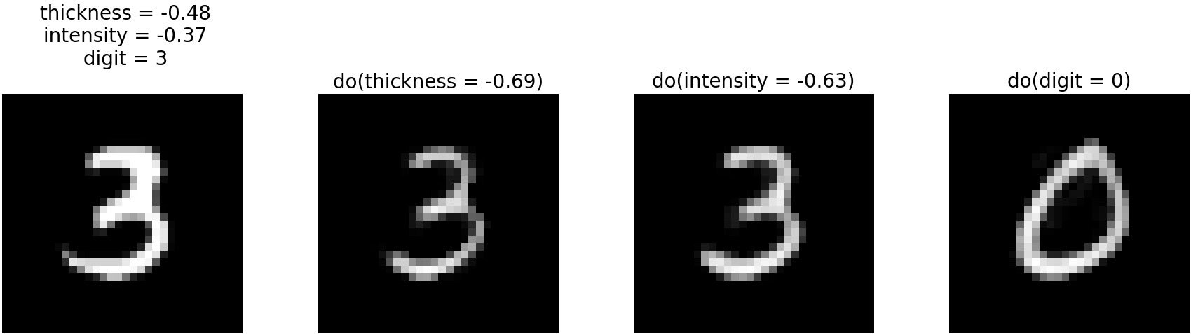
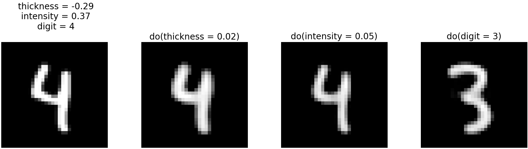
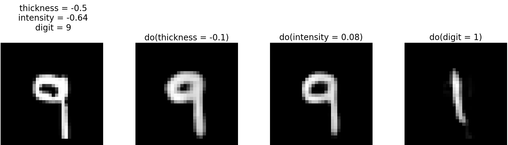
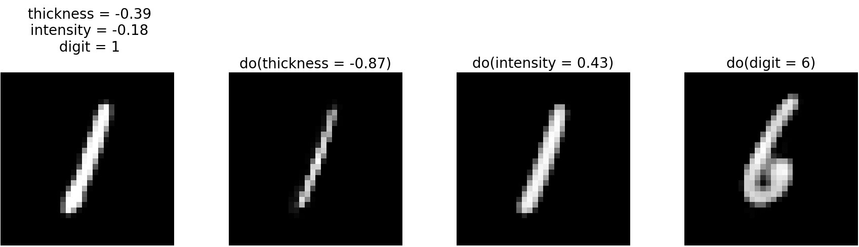
(a) VAE($\sigma=\sqrt{e^{-5}}$)

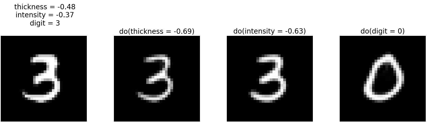
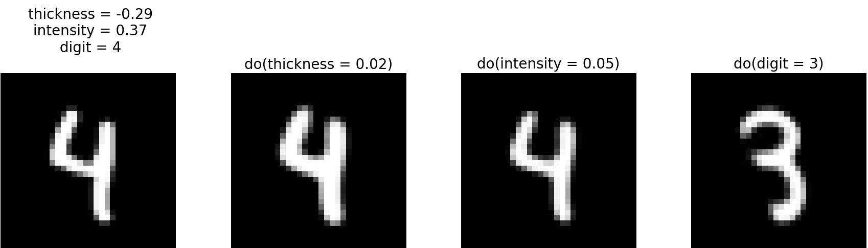
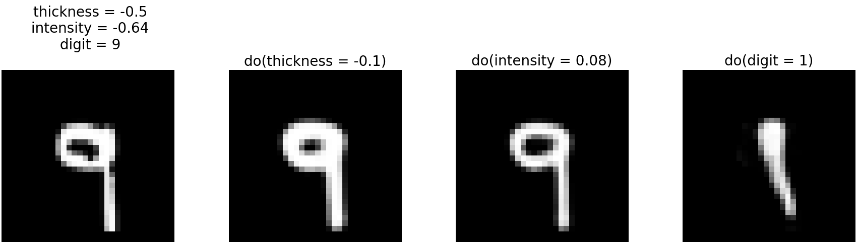
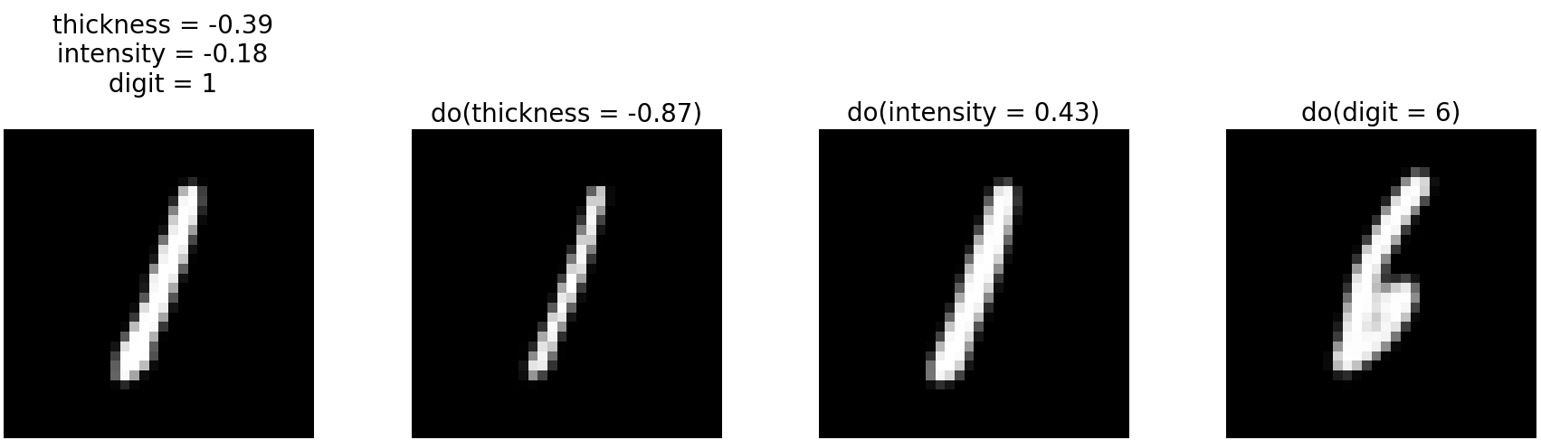
(b) VAE ($\sigma$ learned)

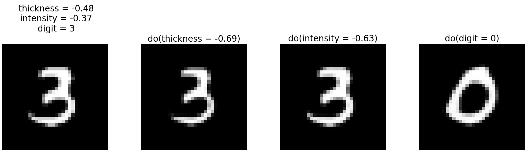
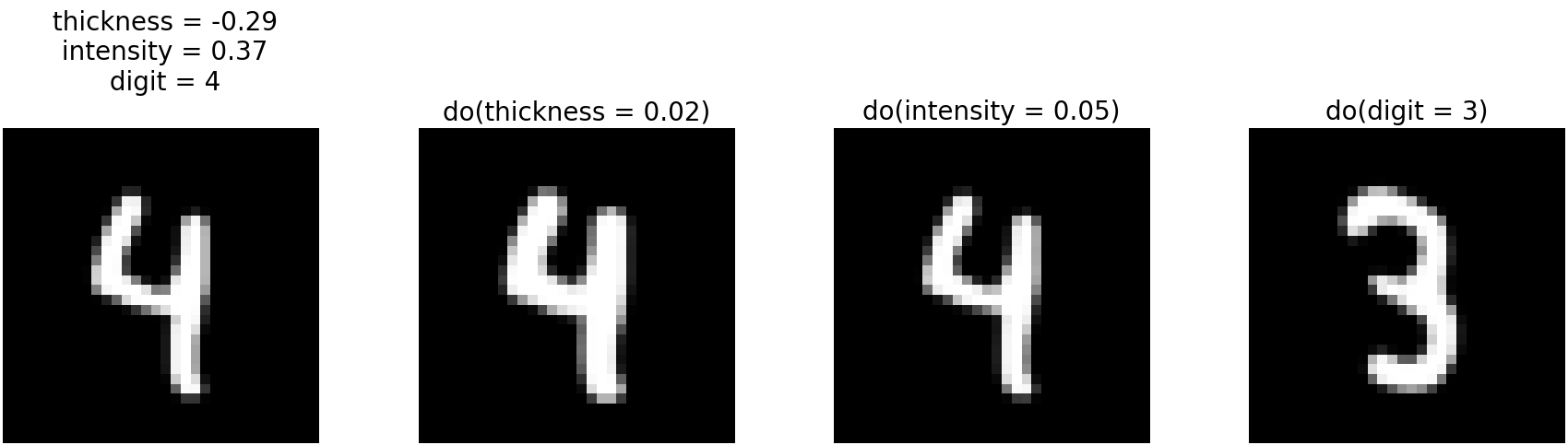
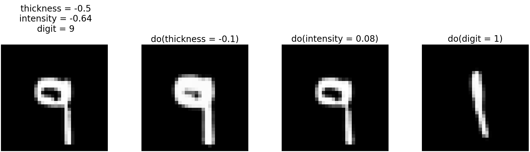
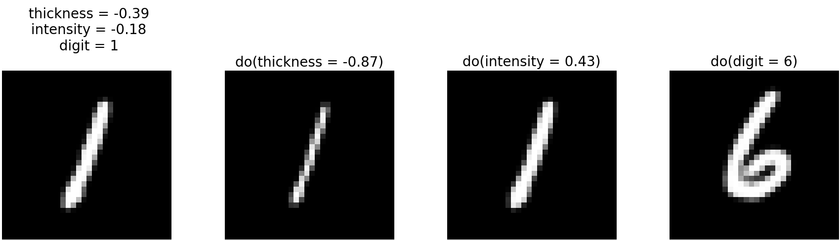
(c) HVAE

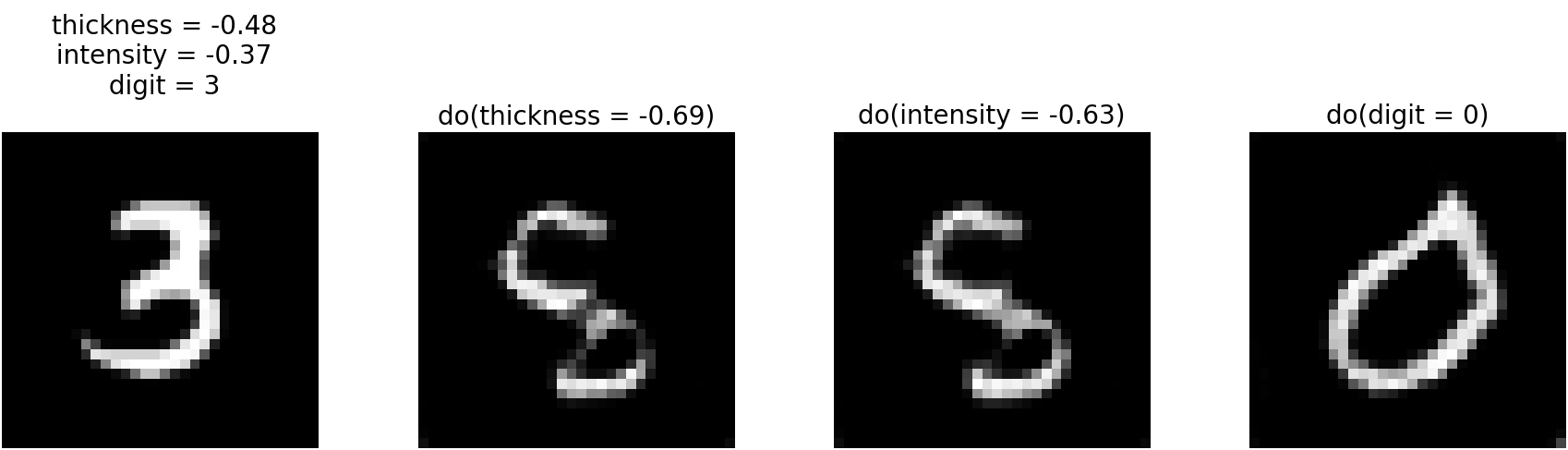
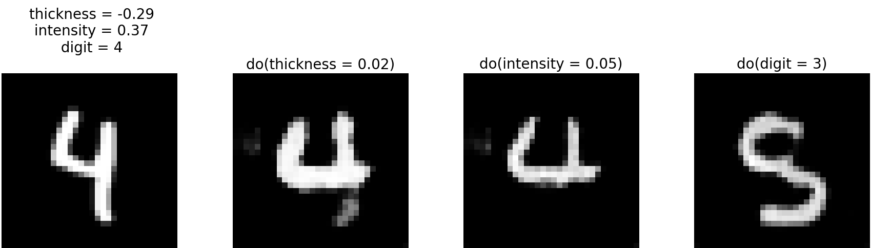
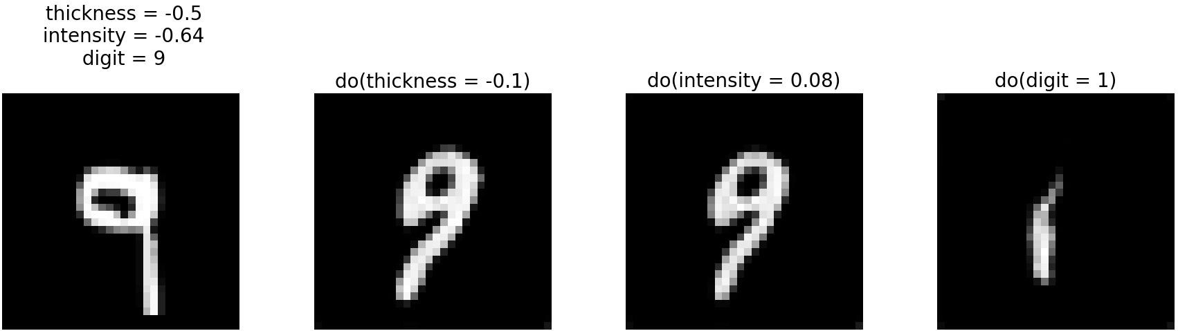
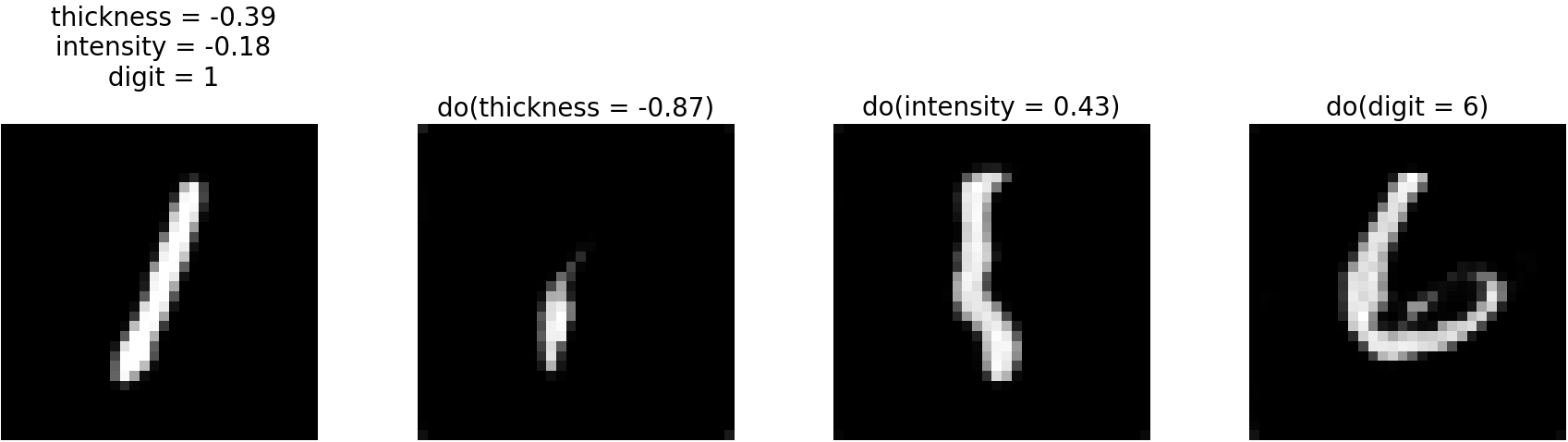
(d) GAN

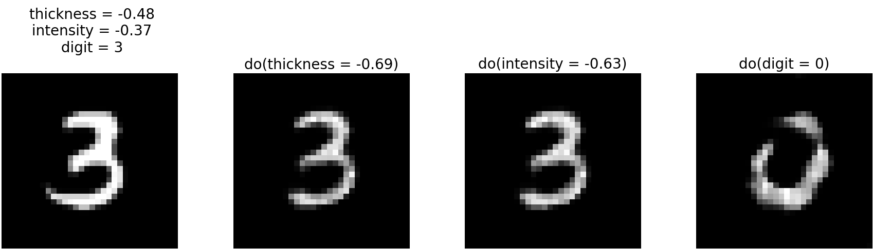
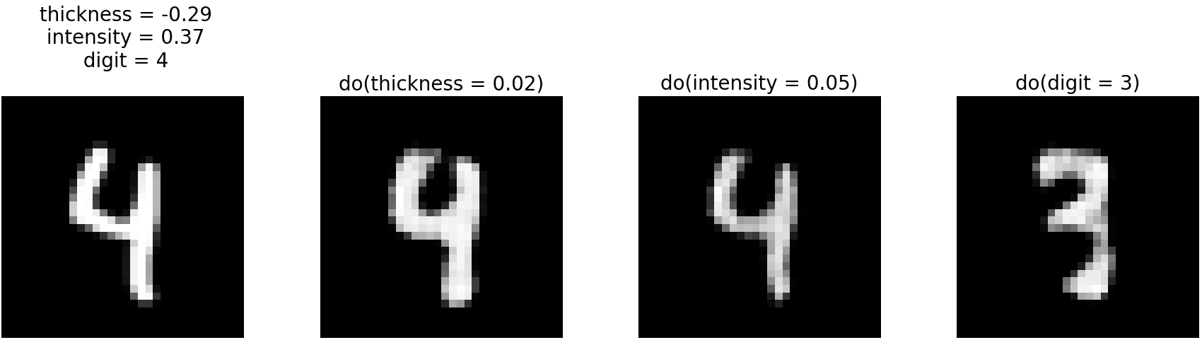
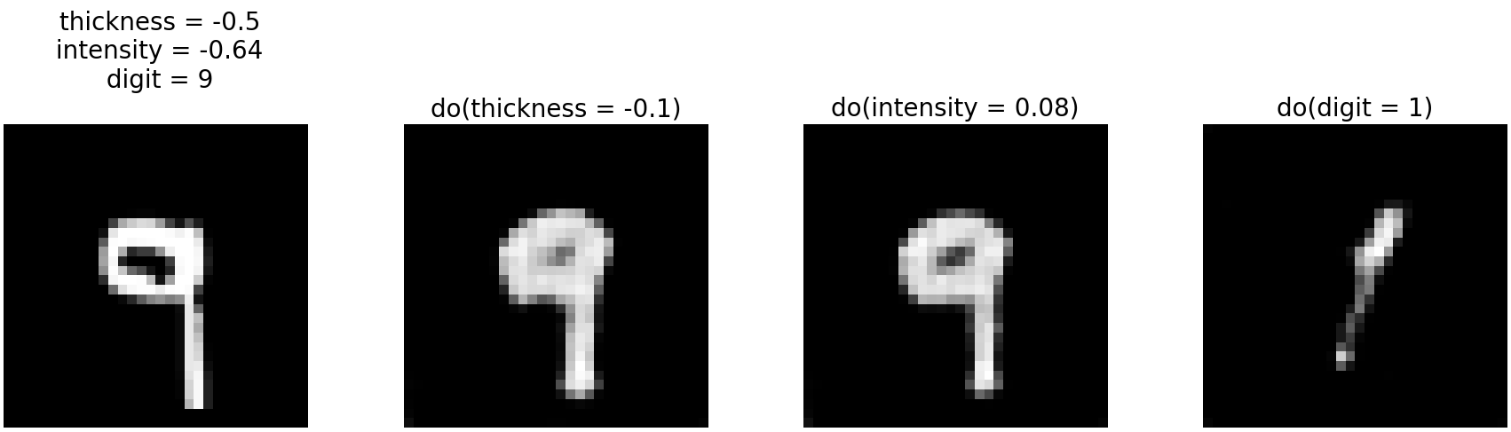
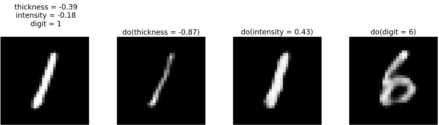
(e) GAN fine-tuned

Figure 7: Interventions on MorphoMNIST.

0.B.2 CelebA

(a) VAE ($\sigma=\sqrt{e^{-5}}$)

(b) VAE ($\sigma$ learned)

(c) HVAE fine-tuned

(d) GAN

(e) GAN fine-tuned

Figure 8: Composition for 10 cycles on the CelebA test set.

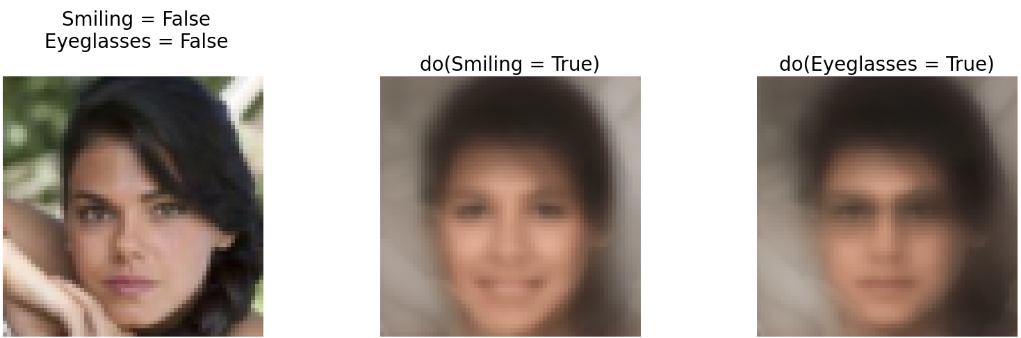
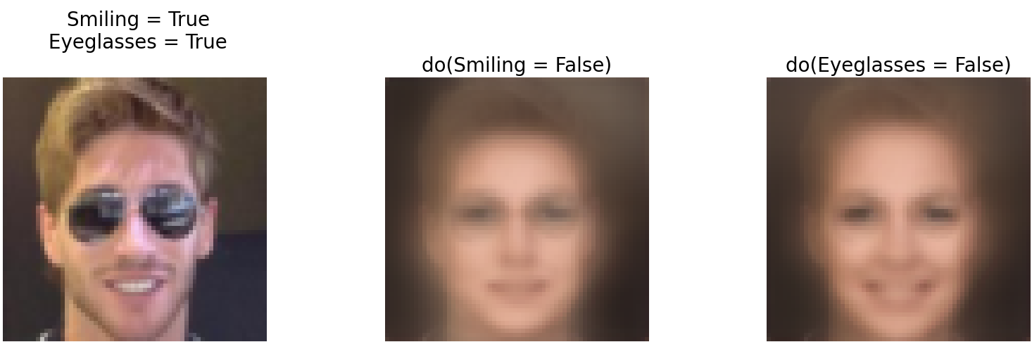
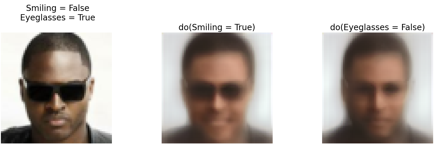
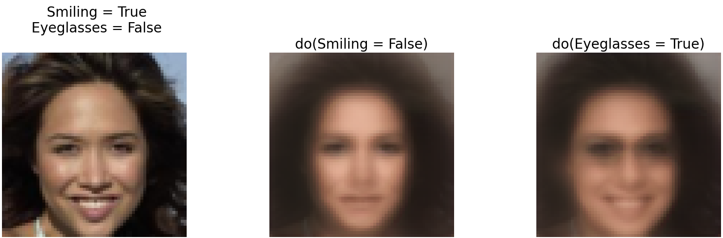
(a) VAE($\sigma=\sqrt{e^{-5}}$)

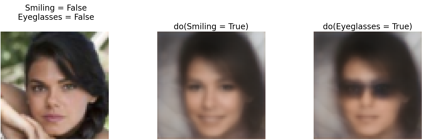
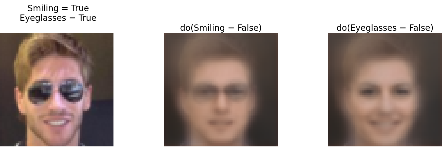
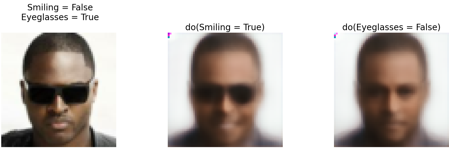
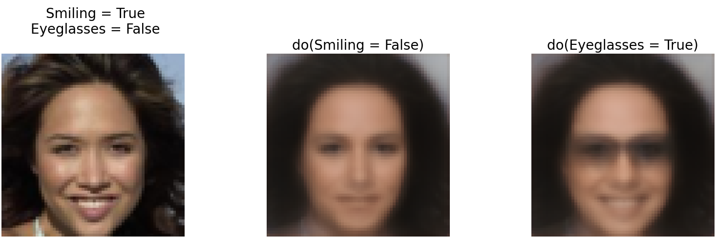
(b) VAE($\sigma$ learned)

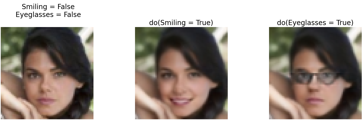
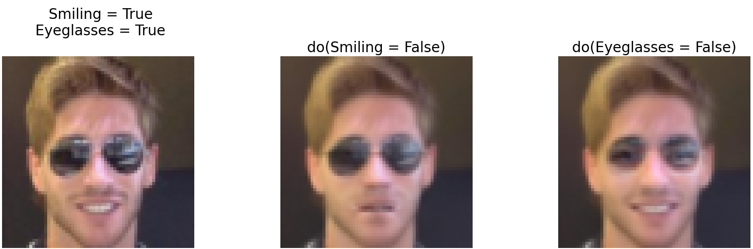
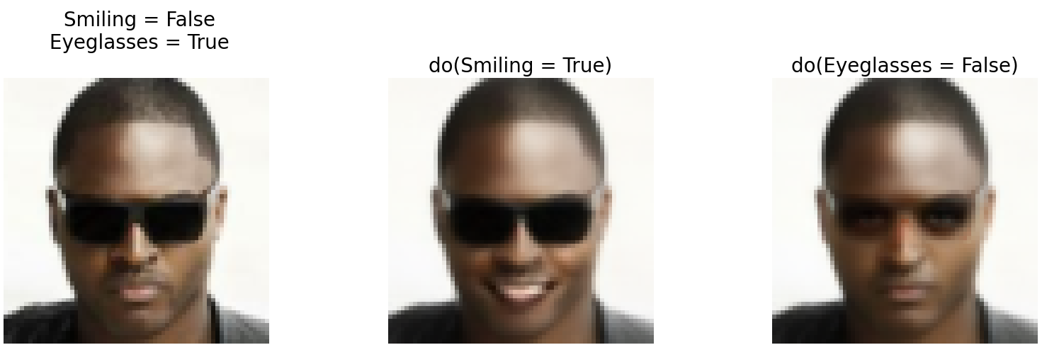
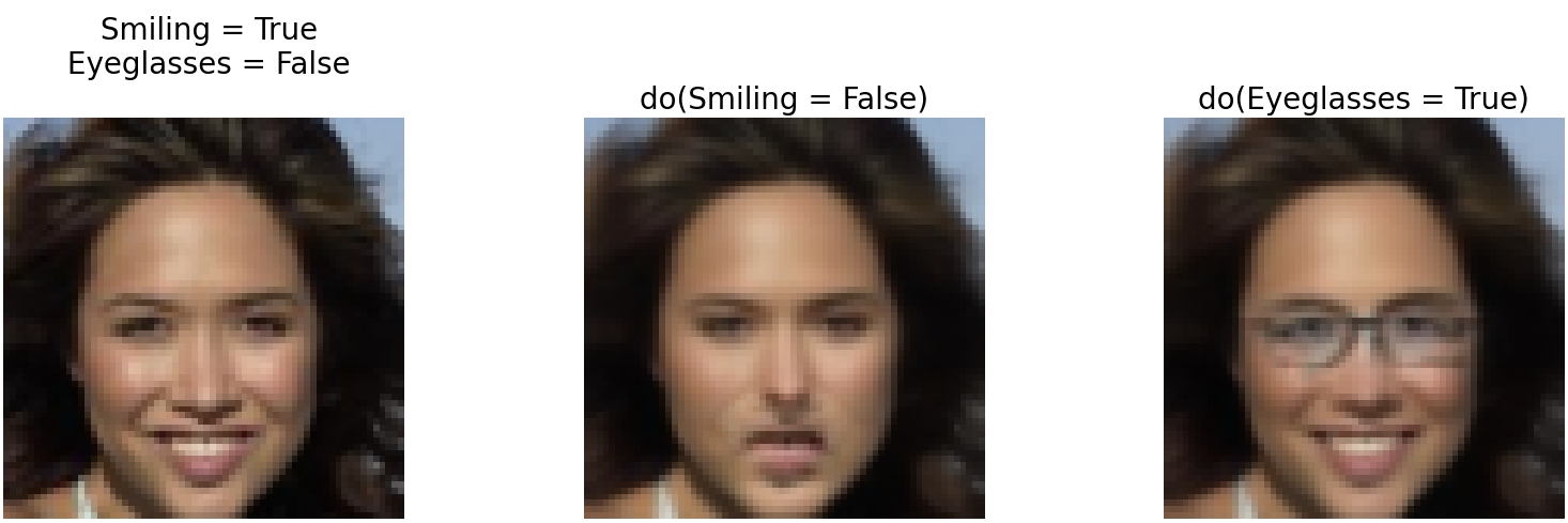
(c) HVAE fine-tuned

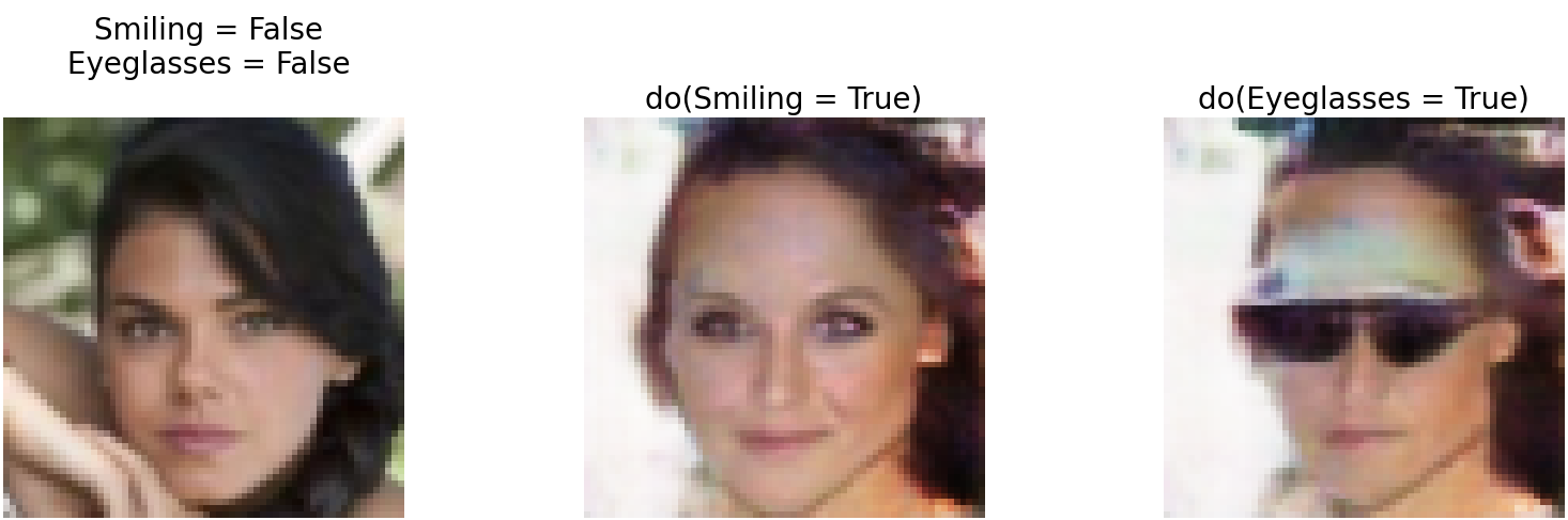
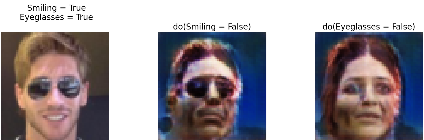
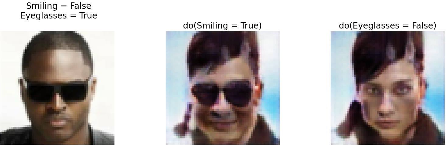
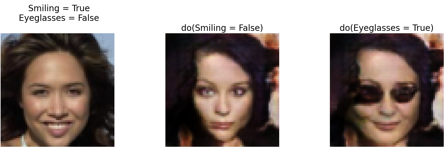
(d) GAN

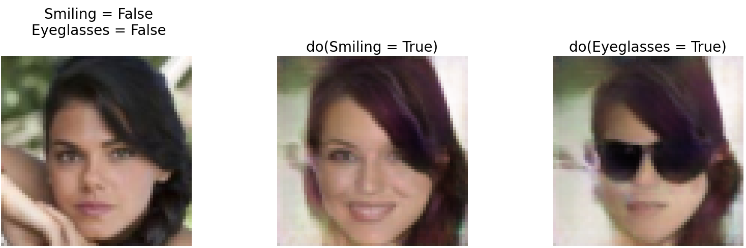
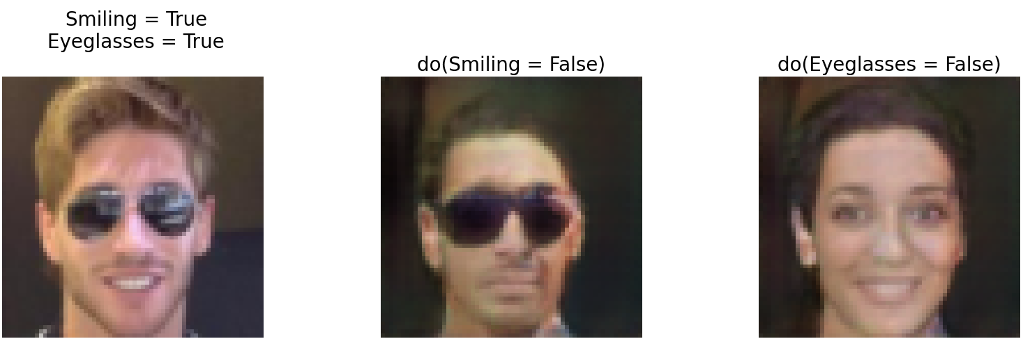
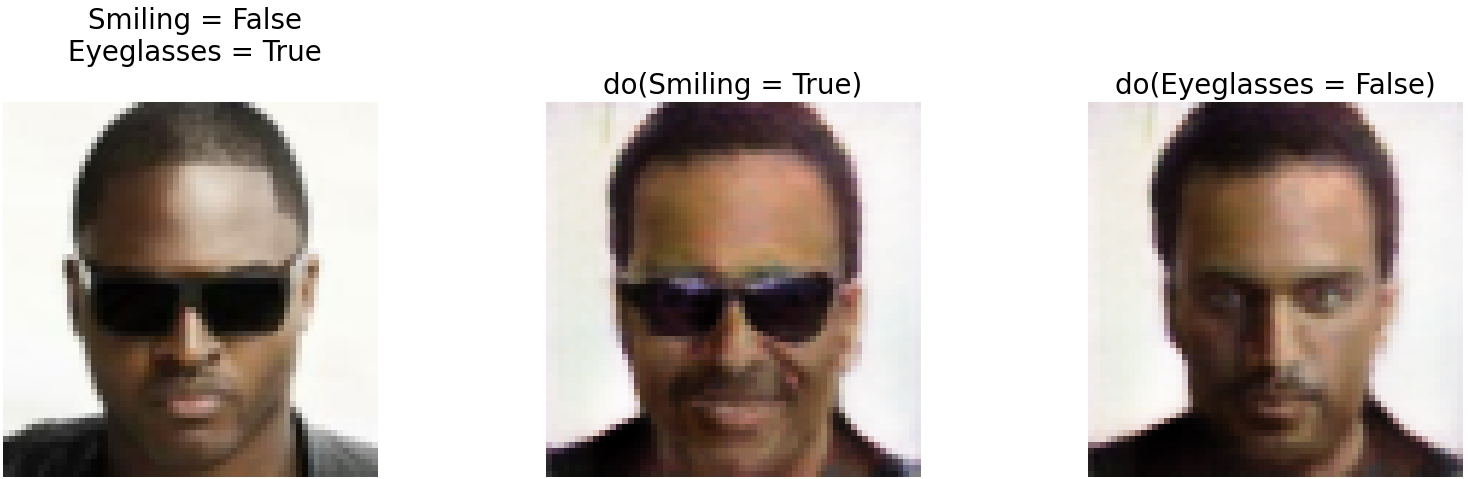
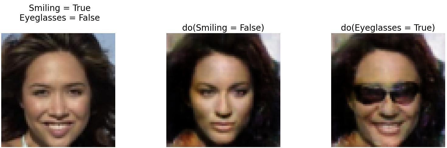
(e) GAN fine-tuned

Figure 9: Interventions on CelebA.

References

- [1] Coelho de Castro, D., Tan, J., Kainz, B., Konukoglu, E., Glocker, B.: Morpho-mnist: Quantitative assessment and diagnostics for representation learning. Journal of Machine Learning Research 20 (10 2019)
- [2] Child, R.: Very deep vaes generalize autoregressive models and can outperform them on images. In: International Conference on Learning Representations (2020)
- [3] Dash, S., Balasubramanian, V.N., Sharma, A.: Evaluating and mitigating bias in image classifiers: A causal perspective using counterfactuals. In: Proceedings of the IEEE/CVF Winter Conference on Applications of Computer Vision (WACV). pp. 915–924 (January 2022)
- [4] De Sousa Ribeiro, F., Xia, T., Monteiro, M., Pawlowski, N., Glocker, B.: High fidelity image counterfactuals with probabilistic causal models. In: Proceedings of the 40th International Conference on Machine Learning. Proceedings of Machine Learning Research, vol. 202, pp. 7390–7425 (23–29 Jul 2023), https://proceedings.mlr.press/v202/de-sousa-ribeiro23a.html
- [5] Dhurandhar, A., Chen, P.Y., Luss, R., Tu, C.C., Ting, P.S., Shanmugam, K., Das, P.: Explanations based on the missing: Towards contrastive explanations with pertinent negatives. In: Neural Information Processing Systems (2018), https://api.semanticscholar.org/CorpusID:3401346
- [6] Dogan, Y., Keles, H.Y.: Semi-supervised image attribute editing using generative adversarial networks. Neurocomputing 401, 338–352 (2020), https://www.sciencedirect.com/science/article/pii/S0925231220304586
- [7] Dumoulin, V., Belghazi, I., Poole, B., Lamb, A., Arjovsky, M., Mastropietro, O., Courville, A.: Adversarially learned inference. In: International Conference on Learning Representations (2017), https://openreview.net/forum?id=B1ElR4cgg
- [8] Escalante, H.J., Escalera, S., Guyon, I., Baró, X., Güçlütürk, Y., Güçlü, U., van Gerven, M.A.J.: Explainable and interpretable models in computer vision and machine learning. The Springer Series on Challenges in Machine Learning, Springer Verlag (Jan 2018). https://doi.org/10.1007/978-3-319-98131-4, https://inria.hal.science/hal-01991623
- [9] Fontanella, A., Mair, G., Wardlaw, J., Trucco, E., Storkey, A.: Diffusion models for counterfactual generation and anomaly detection in brain images (arXiv:2308.02062) (Aug 2023). https://doi.org/10.48550/arXiv.2308.02062, http://arxiv.org/abs/2308.02062, arXiv:2308.02062 [cs, eess]
- [10] Galles, D., Pearl, J.: An axiomatic characterization of causal counterfactuals. Foundations of Science 3, 151–182 (1998)
- [11] Goodfellow, I., Pouget-Abadie, J., Mirza, M., Xu, B., Warde-Farley, D., Ozair, S., Courville, A., Bengio, Y.: Generative adversarial nets. In: Ghahramani, Z., Welling, M., Cortes, C., Lawrence, N., Weinberger, K. (eds.) Advances in Neural Information Processing Systems. vol. 27. Curran Associates, Inc. (2014), https://proceedings.neurips.cc/paper_files/paper/2014/file/5ca3e9b122f61f8f06494c97b1afccf3-Paper.pdf
- [12] Halpern, J.Y.: Axiomatizing causal reasoning. Journal of Artificial Intelligence Research 12, 317–337 (2000)
- [13] Hertz, A., Mokady, R., Tenenbaum, J., Aberman, K., Pritch, Y., Cohen-Or, D.: Prompt-to-prompt image editing with cross attention control (2022)
- [14] Hessel, J., Holtzman, A., Forbes, M., Le Bras, R., Choi, Y.: CLIPScore: A reference-free evaluation metric for image captioning. In: Moens, M.F., Huang, X., Specia, L., Yih, S.W.t. (eds.) Proceedings of the 2021 Conference on Empirical Methods in Natural Language Processing. pp. 7514–7528. Association for Computational Linguistics, Online and Punta Cana, Dominican Republic (Nov 2021). https://doi.org/10.18653/v1/2021.emnlp-main.595, https://aclanthology.org/2021.emnlp-main.595
- [15] Heusel, M., Ramsauer, H., Unterthiner, T., Nessler, B., Hochreiter, S.: Gans trained by a two time-scale update rule converge to a local nash equilibrium. In: Proceedings of the 31st International Conference on Neural Information Processing Systems. p. 6629–6640. NIPS’17, Curran Associates Inc., Red Hook, NY, USA (2017)
- [16] Higgins, I., Matthey, L., Pal, A., Burgess, C.P., Glorot, X., Botvinick, M.M., Mohamed, S., Lerchner, A.: beta-vae: Learning basic visual concepts with a constrained variational framework. In: International Conference on Learning Representations (2016), https://api.semanticscholar.org/CorpusID:46798026
- [17] Ho, J., Jain, A., Abbeel, P.: Denoising diffusion probabilistic models. In: Larochelle, H., Ranzato, M., Hadsell, R., Balcan, M.F., Lin, H. (eds.) Advances in Neural Information Processing Systems. vol. 33, p. 6840–6851. Curran Associates, Inc. (2020), https://proceedings.neurips.cc/paper_files/paper/2020/file/4c5bcfec8584af0d967f1ab10179ca4b-Paper.pdf
- [18] Kaddour, J., Lynch, A., Liu, Q., Kusner, M.J., Silva, R.: Causal machine learning: A survey and open problems. arXiv preprint arXiv:2206.15475 (2022)
- [19] Kaufmann, M.: Causation, action, and counterfactuals (2004), https://api.semanticscholar.org/CorpusID:265038796
- [20] Kingma, D.P., Welling, M.: Auto-Encoding Variational Bayes. In: 2nd International Conference on Learning Representations, ICLR 2014, Banff, AB, Canada, April 14-16, 2014, Conference Track Proceedings (2014)
- [21] Kingma, D.P., Salimans, T., Jozefowicz, R., Chen, X., Sutskever, I., Welling, M.: Improved variational inference with inverse autoregressive flow. Advances in neural information processing systems 29 (2016)
- [22] Kladny, K.R., von Kügelgen, J., Schölkopf, B., Muehlebach, M.: Deep backtracking counterfactuals for causally compliant explanations (2024)
- [23] Kocaoglu, M., Snyder, C., Dimakis, A.G., Vishwanath, S.: Causalgan: Learning causal implicit generative models with adversarial training. In: 6th International Conference on Learning Representations, ICLR 2018, Vancouver, BC, Canada, April 30 - May 3, 2018, Conference Track Proceedings. OpenReview.net (2018), https://openreview.net/forum?id=BJE-4xW0W
- [24] Kügelgen, J.V., Mohamed, A., Beckers, S.: Backtracking counterfactuals. In: van der Schaar, M., Zhang, C., Janzing, D. (eds.) Proceedings of the Second Conference on Causal Learning and Reasoning. Proceedings of Machine Learning Research, vol. 213, pp. 177–196. PMLR (11–14 Apr 2023), https://proceedings.mlr.press/v213/kugelgen23a.html
- [25] Ling, H., Kreis, K., Li, D., Kim, S.W., Torralba, A., Fidler, S.: Editgan: High-precision semantic image editing. In: Advances in Neural Information Processing Systems (NeurIPS) (2021)
- [26] Liu, Z., Luo, P., Wang, X., Tang, X.: Deep learning face attributes in the wild. In: Proceedings of International Conference on Computer Vision (ICCV) (December 2015)
- [27] Lundberg, S.M., Lee, S.I.: A unified approach to interpreting model predictions. In: Guyon, I., Luxburg, U.V., Bengio, S., Wallach, H., Fergus, R., Vishwanathan, S., Garnett, R. (eds.) Advances in Neural Information Processing Systems 30, pp. 4765–4774. Curran Associates, Inc. (2017), http://papers.nips.cc/paper/7062-a-unified-approach-to-interpreting-model-predictions.pdf
- [28] Mirza, M., Osindero, S.: Conditional generative adversarial nets. ArXiv abs/1411.1784 (2014), https://api.semanticscholar.org/CorpusID:12803511
- [29] Mokady, R., Hertz, A., Aberman, K., Pritch, Y., Cohen-Or, D.: Null-text inversion for editing real images using guided diffusion models. In: Proceedings of the IEEE/CVF Conference on Computer Vision and Pattern Recognition (CVPR). pp. 6038–6047 (June 2023)
- [30] Monteiro, M., Ribeiro, F.D.S., Pawlowski, N., Castro, D.C., Glocker, B.: Measuring axiomatic soundness of counterfactual image models. In: The Eleventh International Conference on Learning Representations (2022)
- [31] Pawlowski, N., Castro, D.C., Glocker, B.: Deep structural causal models for tractable counterfactual inference. In: Proceedings of the 34th International Conference on Neural Information Processing Systems. NIPS’20, Curran Associates Inc., Red Hook, NY, USA (2020)
- [32] Pearl, J.: Causality (2nd edition). Cambridge University Press (2009)
- [33] Platt, J., Barr, A.: Constrained differential optimization. In: Neural Information Processing Systems (1987)
- [34] Radford, A., Kim, J.W., Hallacy, C., Ramesh, A., Goh, G., Agarwal, S., Sastry, G., Askell, A., Mishkin, P., Clark, J., Krueger, G., Sutskever, I.: Learning transferable visual models from natural language supervision (2021)
- [35] Reynaud, H., Vlontzos, A., Dombrowski, M., Gilligan-Lee, C.M., Beqiri, A., Leeson, P., Kainz, B.: D’artagnan: Counterfactual video generation. In: Wang, L., Dou, Q., Fletcher, P.T., Speidel, S., Li, S. (eds.) Medical Image Computing and Computer Assisted Intervention - MICCAI 2022 - 25th International Conference, Singapore, September 18-22, 2022, Proceedings, Part VIII. Lecture Notes in Computer Science, vol. 13438, pp. 599–609. Springer (2022), https://doi.org/10.1007/978-3-031-16452-1_57
- [36] Sanchez, P., Kascenas, A., Liu, X., O’Neil, A., Tsaftaris, S.: What is healthy? generative counterfactual diffusion for lesion localization. In: Mukhopadhyay, A., Oksuz, I., Engelhardt, S., Zhu, D., Yuan, Y. (eds.) Deep Generative Models - 2nd MICCAI Workshop, DGM4MICCAI 2022, Held in Conjunction with MICCAI 2022, Proceedings. pp. 34–44. Lecture Notes in Computer Science (including subseries Lecture Notes in Artificial Intelligence and Lecture Notes in Bioinformatics), Springer Science and Business Media Deutschland GmbH, Germany (Oct 2022). https://doi.org/10.1007/978-3-031-18576-2_4
- [37] Sanchez, P., Tsaftaris, S.A.: Diffusion causal models for counterfactual estimation. In: CLEaR (2022), https://api.semanticscholar.org/CorpusID:247011291
- [38] Sauer, A., Geiger, A.: Counterfactual generative networks. In: International Conference on Learning Representations (2021), https://openreview.net/forum?id=BXewfAYMmJw
- [39] Schölkopf, B., Locatello, F., Bauer, S., Ke, N.R., Kalchbrenner, N., Goyal, A., Bengio, Y.: Towards causal representation learning. ArXiv abs/2102.11107 (2021), https://api.semanticscholar.org/CorpusID:231986372
- [40] Schölkopf, B., Locatello, F., Bauer, S., Ke, N.R., Kalchbrenner, N., Goyal, A., Bengio, Y.: Toward causal representation learning. Proceedings of the IEEE 109(5), 612–634 (2021). https://doi.org/10.1109/JPROC.2021.3058954
- [41] Sø nderby, C.K., Raiko, T., Maalø e, L., Sø nderby, S.r.K., Winther, O.: Ladder variational autoencoders. In: Lee, D., Sugiyama, M., Luxburg, U., Guyon, I., Garnett, R. (eds.) Advances in Neural Information Processing Systems. vol. 29. Curran Associates, Inc. (2016), https://proceedings.neurips.cc/paper_files/paper/2016/file/6ae07dcb33ec3b7c814df797cbda0f87-Paper.pdf
- [42] Song, J., Meng, C., Ermon, S.: Denoising diffusion implicit models. In: International Conference on Learning Representations (2021), https://openreview.net/forum?id=St1giarCHLP
- [43] Szegedy, C., Liu, W., Jia, Y., Sermanet, P., Reed, S.E., Anguelov, D., Erhan, D., Vanhoucke, V., Rabinovich, A.: Going deeper with convolutions. In: IEEE Conference on Computer Vision and Pattern Recognition, CVPR 2015, Boston, MA, USA, June 7-12, 2015. pp. 1–9. IEEE Computer Society (2015), https://doi.org/10.1109/CVPR.2015.7298594
- [44] Tabak, E., Cristina, T.: A family of nonparametric density estimation algorithms. Communications on Pure and Applied Mathematics 66 (02 2013). https://doi.org/10.1002/cpa.21423
- [45] Taylor-Melanson, W., Sadeghi, Z., Matwin, S.: Causal generative explainers using counterfactual inference: A case study on the morpho-mnist dataset. ArXiv abs/2401.11394 (2024), https://api.semanticscholar.org/CorpusID:267069516
- [46] Trippe, B.L., Turner, R.E.: Conditional density estimation with bayesian normalising flows. arXiv: Machine Learning (2018), https://api.semanticscholar.org/CorpusID:88516568
- [47] Vahdat, A., Kautz, J.: Nvae: A deep hierarchical variational autoencoder. Advances in neural information processing systems 33, 19667–19679 (2020)
- [48] Van Looveren, A., Klaise, J.: Interpretable counterfactual explanations guided by prototypes. In: Oliver, N., Pérez-Cruz, F., Kramer, S., Read, J., Lozano, J.A. (eds.) Machine Learning and Knowledge Discovery in Databases. Research Track. p. 650–665. Springer International Publishing, Cham (2021)
- [49] Vlontzos, A., Kainz, B., Gilligan-Lee, C.M.: Estimating categorical counterfactuals via deep twin networks. Nature Machine Intelligence 5(2), 159–168 (2023)
- [50] Vlontzos, A., Rueckert, D., Kainz, B., et al.: A review of causality for learning algorithms in medical image analysis. Machine Learning for Biomedical Imaging 1(November 2022 issue), 1–17 (2022)
- [51] Yang, M., Liu, F., Chen, Z., Shen, X., Hao, J., Wang, J.: Causalvae: Disentangled representation learning via neural structural causal models. 2021 IEEE/CVF Conference on Computer Vision and Pattern Recognition (CVPR) pp. 9588–9597 (2020), https://api.semanticscholar.org/CorpusID:220280826
- [52] Zečević, M., Willig, M., Dhami, D.S., Kersting, K.: Identifying challenges for generalizing to the pearl causal hierarchy on images. ICLR 2023 Workshop on Domain Generalization (Apr 2023), https://openreview.net/forum?id=QBgmo9BvnS
- [53] Zhang, R., Isola, P., Efros, A.A., Shechtman, E., Wang, O.: The unreasonable effectiveness of deep features as a perceptual metric. In: Proceedings of the IEEE conference on computer vision and pattern recognition. pp. 586–595 (2018)
- [54] Zou, S., Tang, J., Zhou, Y., He, J., Zhao, C., Zhang, R., Hu, Z., Sun, X.: Towards efficient diffusion-based image editing with instant attention masks (2024)