Infinitesimal calculations in fundamental groups
Abstract.
We show that Hopf invariants, defined by evaluation in Harrison cohomology of the commutative cochains of a space, calculate the logarithm map from a fundamental group to its Malcev Lie algebra. They thus present the zeroth Harrison cohomology as a universal dual object to the Malcev Lie algebra. This structural theorem supports explicit calculations in algebraic topology, geometric topology and combinatorial group theory. In particular, we give the first algorithm to determine whether a word raised to some power is a -fold nested product of commutators, in any group presented by generators and relations.
To the memory and loved ones of the second author.
1. Introduction
We fully develop the capacity of rational or real cochains to measure a fundamental group, and thus any algebraically presented group, through a variety of perspectives.
-
•
In algebraic topology, we establish that Harrison cohomology in degree zero serves as a universal rational Lie dual of a group, equipped with an explicit pairing. It thus provides “coordinates” for the infinitesimal approximation of a group given by the logarithm map from a group to its Malcev Lie algebra.
-
•
Geometrically, intersection of a loop with codimension one subspaces of a manifold, tracking the ordering of meeting times, can be used to define functions on a fundamental group. The theory thus extends non-abelian intersection theory [Hai85], as well as Cochran’s development of Milnor’s link invariants [Coc90]. We initiate the art of finding suitable subspaces and analyzing them through many examples in Section 5, with an emphasis on two-complexes (thickened to four-manifolds) as well as Milnor invariants, which will be fully developed in a sequel.
-
•
Our first full application is in combinatorial group theory. For algebraically presented groups, the theory leads directly to letter-braiding and letter-linking invariants, which generalize Magnus expansion and Fox calculus to all groups. We determine an explicit set of functions on a presented group which obstruct whether some power of a word lies in a desired -fold commutator subgroup. These functions are algorithmic, and have been implemented in SAGE by the second author.
The appearance of Malcev Lie algebras as fundamental groups in rational homotopy theory is classical [Qui69] (see [Iva22] for a recent review). But standard approaches produce an abstractly presented Lie algebra, without comparison to the group. They give no way to answer questions such as determining Malcev filtration degree of specific group elements.
Our work produces an explicit pairing between a group and a central object in one of the Quillen approaches to rational homotopy theory, namely the zeroth Harrison cohomology of a space with that fundamental group. With this pairing, one is able to compute the depth of some in the rational lower central series of . Classical algebraic presentation through generators and relations are reflected in the topology of two-dimensional CW complexes. Their analysis gives rise to a lifting criterion (Theorem 4.7), which in turn gives rise to an algorithm which determines whether or not some power of a word is a product of nested -fold commutators. We introduce the invariants which constitute the algorithm in Section 1.2 below.
While computational algebra is currently our most developed application, the theory is ripe for a wide range of applications, as we address in Section 1.4.3. To study a group through these “coordinates”, one has freedom in choosing a space which presents it as a fundamental group, a flavor of and model for rational (or real) cochains, a presentation of Harrison cohomology, and additional flexibility by considering maps between spaces. The resulting ”charts” can look different for two algebraic presentations of the same group (see Section 5.1) and have a different flavor altogether in topological examples (Sections 5.2 and 5.5). The main construction, that of the Hopf pairing, is simple and natural enough that it should generalize to many settings.
We elaborate on the three main perspectives for our results below. In Section 1.1, we share the framework for results which comes from algebraic topology. In Section 1.2 we share our first applications, to combinatorial group theory. In Section 1.3 we share basic motivating examples, which come from geometric topology. We have written these independently, to be read in any order. Readers are encouraged to explore their favorite “side of the elephant”111https://www.flickr.com/photos/loxosceles/2334950809 first.
1.1. Algebraic topology
We first recall some basic facts about Malcev Lie algebras. The Baker-Campbell-Hausdorff expansion for the logarithm of a product of exponentials in a noncommutative algebra is
where .
The Malcev Lie algebra of a group is a complete Lie algebra equipped with a function such that
| (1) |
satisfying the universal property that any function satisfying (1) into a nilpotent Lie algebra factors uniquely through a Lie algebra homomorphism . This is the completed Lie algebra topologically generated by the elements , subject only to the relations coming from (1).
Quillen in [Qui69] presented as the set of primitive elements in the group ring completed at the ideal generated by for all , with .
In this paper we carefully develop and apply a dual notion to . With suitable finiteness, functions on a Lie algebra inherit the dual structure of a Lie coalgebra. Such coalgebras can be briefly understood as vector spaces equipped with a cobracket such that the dual space naturally forms a Lie algebra. We develop cofree Lie coalgebras carefully in Section 2.
Definition 1.1.
A pairing of a Lie coalgebra with the Malcev Lie algebra is a Lie pairing with if
where on the left pairs with by .
Such a pairing is universal if for any other Lie pairing there exists a unique homomorphism of Lie coalgebras such that
A Lie coalgebra equipped with a universal Lie pairing with is called the Lie dual of . It is unique up to unique isomorphism.
Lie pairings extend the notion of linear functionals on as follows. If satisfies then the pairing with automatically vanishes on all commutators in . It follows that
| (2) |
so the Lie pairing with defines a rational functional on the abelianization of . The kernel of the cobracket of a Lie coalgebra is called the weight zero subspace (see Proposition 2.7). By Equation (2) a Lie pairing restricts to a bilinear pairing of between the weight zero subspace and the abelianization of . In other words, a Lie pairing naturally extends homomorphisms from to , and as we show below, the Lie dual of must have weight zero subspace canonically isomorphic to .
When is finite dimensional, a universal Lie pairing on defines an isomorphism of Lie algebras . But when is infinite dimensional, the Lie dual is distinct from the standard linear dual of , which is no longer a Lie coalgebra.
Lie colagebras arise naturally in studying commutative differential graded algebras, and in particular commutative cochain complexes. Given a commutative augmented differential graded algebra , Harrison constructed a cochain complex computing the derived indecomposables (see Definition 2.8 and Theorem A.4). Surprisingly, these naturally form a Lie coalgebra, the central example for operadic Koszul-Moore duality [Sin13]. Rational homotopy theory relates the Harrison cohomology of a commutative cochain model for a topological space with the linear dual of rational homotopy groups of , matching the Lie coalgebraic structures on both sides.
The third and fourth authors made this effective for higher homotopy groups in the simply connected setting in [SW13]. The present work extends this to fundamental groups, first showing in Proposition 2.11 that there exists a canonical isomorphism . This canonical isomorphism gives rise to the Hopf invariant pairing between and via pull-back and evaluation. The value of some Harrison cocycle on some is given by . Our main structural result is the following.
Theorem 1.2.
Let be a pointed simplicial set or differentiable manifold and the de Rham (PL or smooth, respectively) cochains on . The Hopf invariant pairing defined by
is a univeral Lie pairing of with .
Thus the zeroth Harrison cohomology of is the natural Lie extension of the evaluation of cohomology on homotopy, where . While conceptually satisfying, the true value of this theorem is that the right hand side can be explicitly analyzed. Whenever a fundamental group is tied to a space of interest, or such a space can be found, Harrison cohomology provides a means for calculations in its Malcev Lie algebra. We provide applications in algebra and geometric topology, as explained next.
1.2. Combinatorial group theory
Our framework leads to a remarkably elementary combinatorial approach to understanding the radical of the lower central series of presented groups.
Definition 1.3.
A finite discrete function, or d-function, is a function from to an abelian group, here exclusively the additive group of the rational numbers. If is a d-function, define to be the sum .
Definition 1.4.
Consider a word where are generators of a free group and . If is a homomorphism let be the d-function .
Thus , the evaluation of a homomorphism. We construct below a derived version of evaluation which we call letter braiding functions, built from a discrete version of iterated integrals.
Definition 1.5.
Given , a word of length , for each let where is either if or else if . If and are two d-functions with domain , define to be the function given by partial sums . The braiding product of and is the point-wise product .
See Example 1.8 below. The braiding product terminology will be explained below in Section 3.2, where we will see that the definition of is dictated by topology.
Definition 1.6.
A formal braiding symbol in some set of formal variables, say is, inductively, a formal linear combination of expressions each of which is either a variable or has the form or , where and are symbols. The weight of a symbol is the largest number of formal braiding products which occur in a term of the linear combination.
A braiding symbol is a pair where is a formal braiding symbol and are homomorphisms .
In examples, we shorten notation by incorporating homomorphisms in the symbol – for example stands for the braiding symbol .
Braiding symbols give recipes for specifying d-functions associated to any word.
Definition 1.7.
If is a braiding symbol and is a word of length , the associated d-function is obtained by performing the prescribed braiding products recursively
starting with as defined above, and extending linearly for linear combinations. The value of the symbol on is . We call the assignment the letter braiding function associated to the symbol .
Example 1.8.
Suppose in . Let be the indicator homomorphism which sends and the other generators to zero; let and be defined similarly. The table below gives a step-by-step computation of the braiding product . The caret marks in the row for indicate the final term of the corresponding partial sum, dictated by ending at either or .
We deduce that .
We omit the short, elementary proof of the following basic fact.
Proposition 1.9.
Letter braiding functions on words descend to well-defined functions on free groups.
While letter braiding functions are elementary combinatorial objects, we will connect them with larger frameworks from geometry and rational homotopy theory under conditions we call the “eigen setting,” where multiple approaches of invariant functions on groups coincide and have integer values. One such theory consists of the subset of letter braiding functions with all proper subsymbols vanishing (see Definition 3.1), which are called letter linking functions.
Letter linking functions are the subject of [MS22], whose main result is that letter linking functions associated to symbols decorated by indicator homomorphisms – those which take some generator to one and all others to zero – are sharp obstructions the lower central series of free groups. For example , as there is one in between an pair. Since the ’s and ’s have a non-zero “linking number”, the word is not a two-fold commutator.
One of our main present results is to generalize this to the radical of the lower central series for all groups. Let present a group as a quotient of a free group , and say a letter linking function of descends to if the function is constant on cosets of . Our Lifting Theorem below (see Section 4.2) characterizes the letter linking functions that descend to a quotient group. Clearly, such functions must vanish on relations in , but this is insufficient. Our theorem gives a complete criterion using the language of Lie coalgebras, developed in Section 2. We then have the following main theorem.
Theorem 1.10.
Let be a word representing an element of . Then some power of is a product of -fold nested commutators in if and only if all weight letter linking functions that descend to vanish on .
When this simply states that the subgroup of on which all homomorphisms to vanish is radical of the commutator subgroup . The cases are all new. Moreover, this along with the Lifting Theorem then give rise to an algorithm to determine whether some power of a word is a -fold commutator, which has been implemented – see Section 4.3.
1.3. Geometric topology
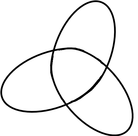
The geometric genesis of our work is illustrated in an elementary analysis of the Borromean rings, which are depicted in Figure 1(a).
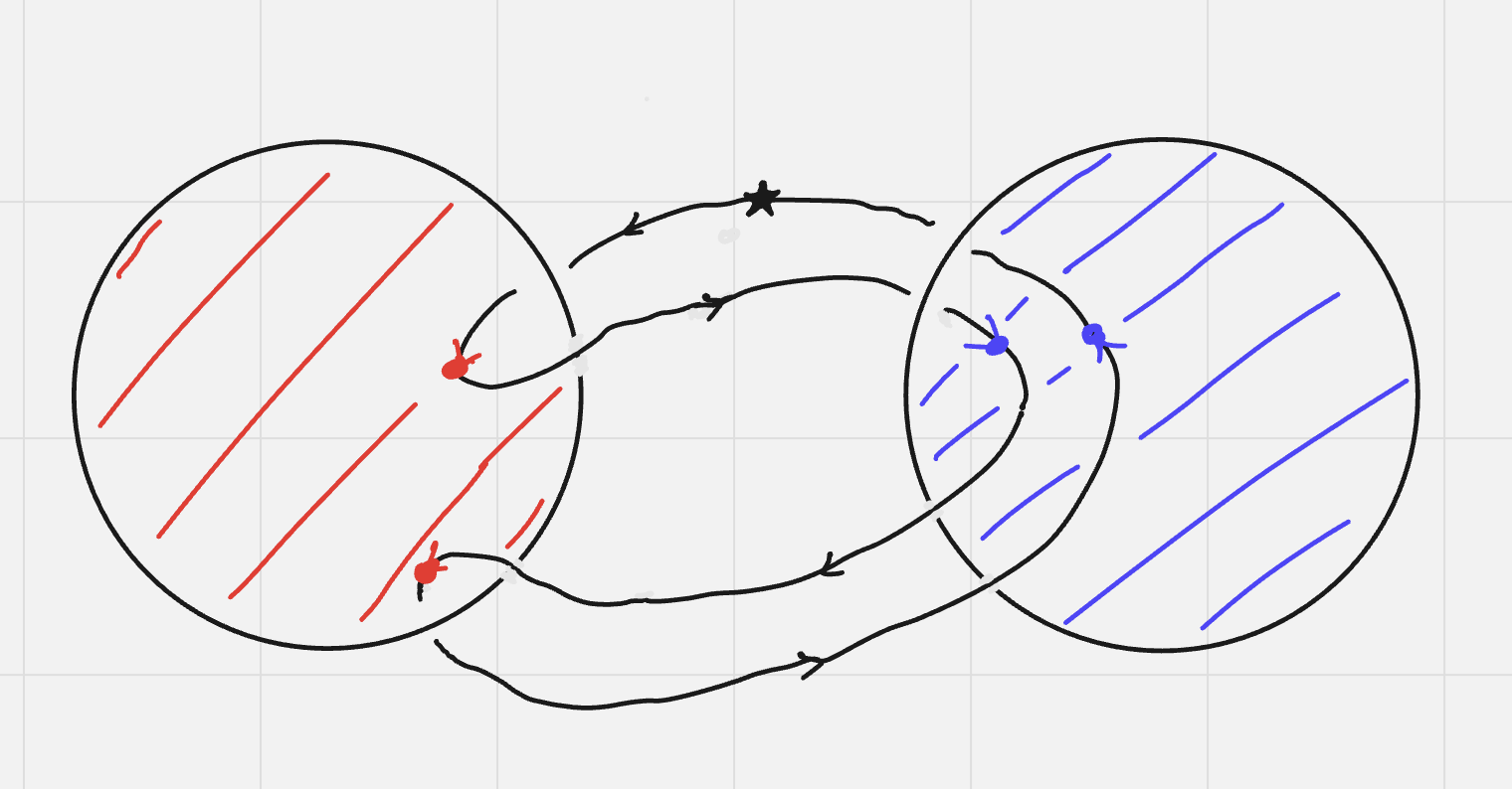
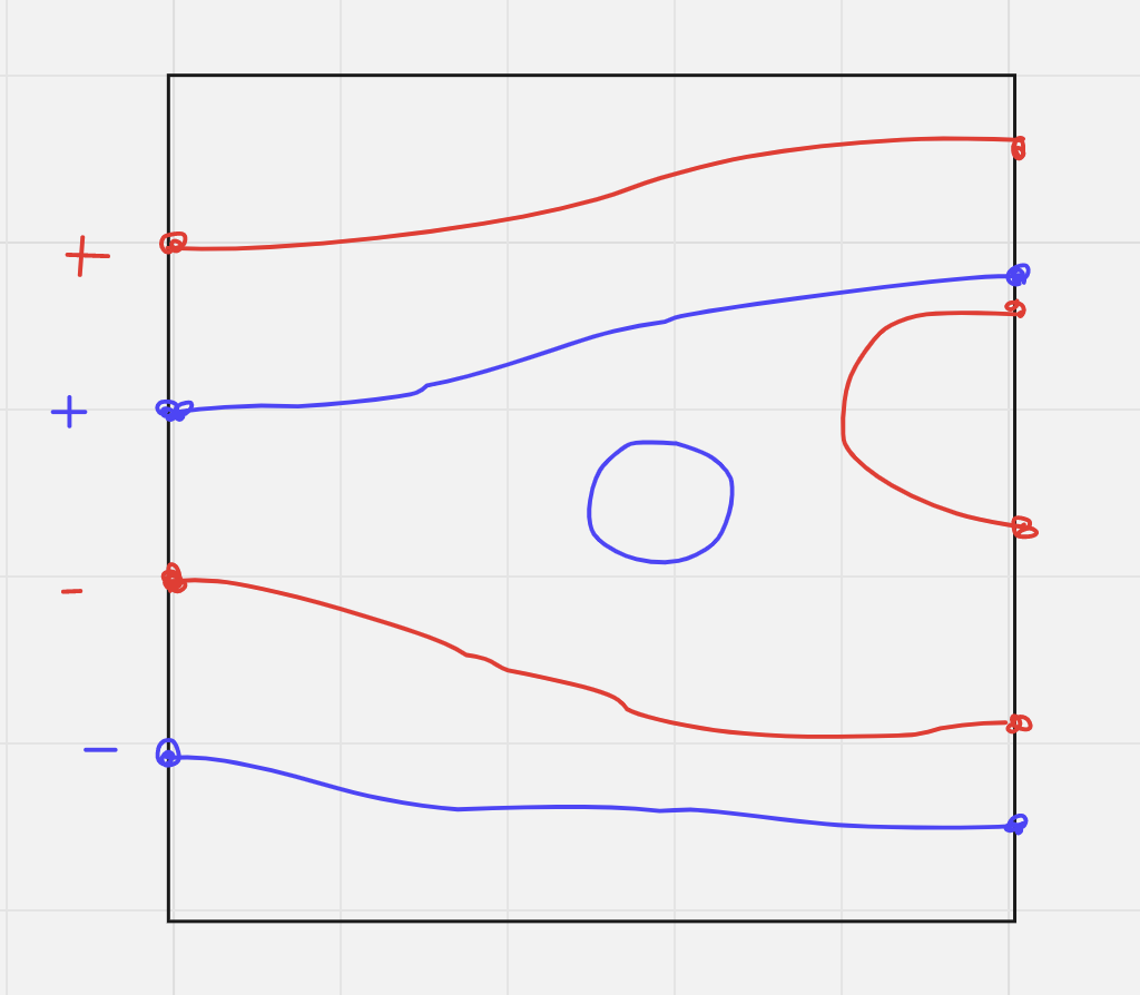
Here two components have Seifert surfaces chosen, in red and blue. We record intersections of the third component with those surfaces on the left edge of the square in Figure 1(b), which represents the domain of that component. These four intersections alternate between red and blue, with signs determined by whether the third component is coming out of or into the page. These signs alternate, and in fact the third component represents a simple commutator in the fundamental group of the first two components.
The square in Figure 1(b) represents the behavior of such intersections under an imagined isotopy of the third component. Assuming transversality throughout, the preimage of the two Seifert surfaces would be curves, pictured in red and blue, which are disjoint. Because the colors of the left ends of these curves alternate, and the curves are disjoint, all four curves must have endpoints on the right edge. So a homotopy of this component pulling it away and resulting in the unlink is impossible. (The Isotopy Extension Theorem can now be invoked to complete a proof that the Borromean rings are linked.)
Hopf invariants can measure elements of fundamental groups by tracking intersections with codimension one submanifolds, for example these Seifert surfaces. Cohomology does this though signed counts of intersection points. The example above illustrates the use of finer combinatorial structure – the interleaving of intersection times – in a case where the simple counts vanish.
We will focus further on the occurrence of blue points between cancelling pairs of red points, the count of which is invariant in this situation and also obstructs pulling away the third component. Similar counts are at the heart of letter linking [MS22], as we introduced in Section 1.2 and will connect to topology in Section 3.2. There are two directions of generalization of such counts. One is that the idea can be iterated. Imagine for example another unknot component, with its Seifert surface say colored green, so the preimages of intersections with surfaces are colored red, blue or green. Then counts of say some green point in between cancelling pairs of blue points which themselves are between cancelling pairs of red points will also define a homotopy invariant of the last component. Such counts will correspond to higher weight Hopf invariants.
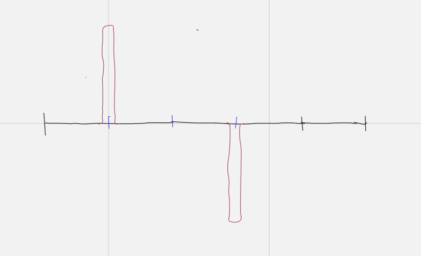
The second direction of generalization is to relax the disjointness of Seifert surfaces needed for the argument above. Consider a Whitehead link, as pictured in Figure 2(a), and imagine a third component linking with it. Since the red and blue surfaces intersect, the order in which the third component intersects them can change.
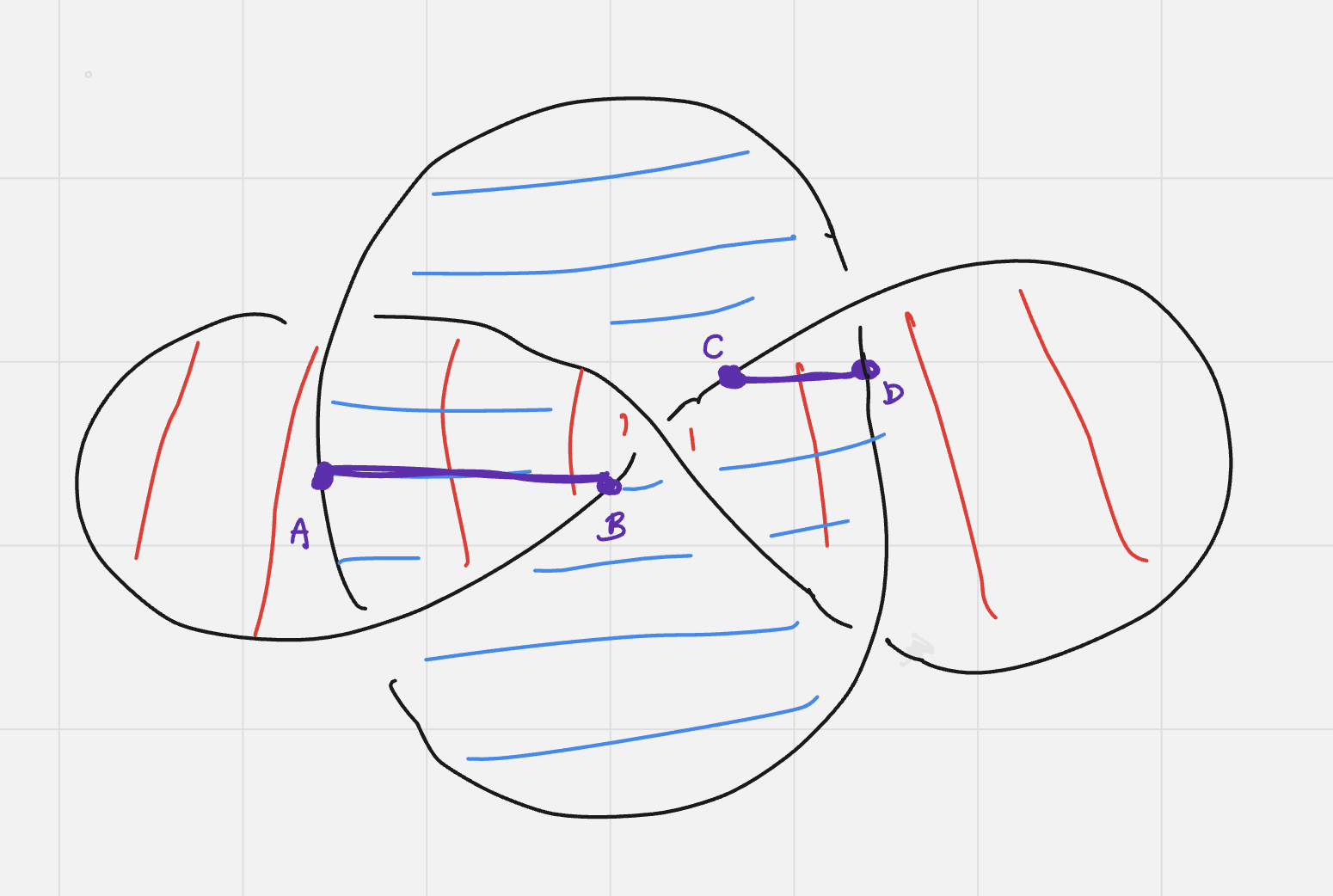
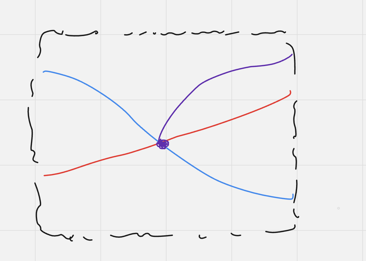
But we can consider an auxiliary surface which bounds their intersection, pictured as the purple segments in Figure 2(a), along with the part of one component running from point to and the part of the other component running from to . If we track intersections of a third link component both with the two Seifert surfaces and this auxiliary surface, say in purple, we would see phenomena such as in Figure 2(b). Here red and blue preimages of intersections cross, which happens where the Seifert surfaces intersect, but their crossing point is a boundary point for the preimage curve for the purple surface. So as the order of intersections with blue and red Seifert surfaces changes – reading left to right the blue intersection goes from being before red to after red — an intersection with the purple surface is created or destroyed. Thus intersections with the purple surface can be used as correction terms for finer counts of blue and red point which depend on order.
Another case worth considering is the Hopf link, for which no there can be no such correction term. Indeed, we can recognize two Seifert surfaces as generators of first cohomology of the complement of the Hopf link, and the non-triviality of their cup product implies there is not a surface in the complement which bounds their intersection (along with sub-curves of the components).
In general the role of submanifolds and their intersections is formalized using the language of Thom forms, as reviewed in Appendix B.1. Suppose is a three-manifold such as a link complement, so surfaces have associated one-forms. Wedge product corresponds to intersection, and the behavior of the product determines whether two surfaces can be used for “counting alternating preimages”. If the product is zero at the cochain level, there is immediately such an invariant. If it is homologous to zero then there is an invariant involving a correction surface. And if the product is non-zero in cohomology then there is no such invariant.
More generally, given a collection codimension one submanifolds one can count preimages of them in prescribed orders. Such counts are generally not invariant, as the codimension one submanifolds can intersect as the Seifert surfaces for the Whithead link do. But one can find linear combinations which are invariant through analysis of these intersections and their relations, which encode cup products and Massey products. Remarkably, this story is governed by a classical constructions from algebra and rational homotopy theory: the bar complex and the Harrison complex. The Harrison theory distinguishes fundamental group elements up to their images in the Malcev Lie algebra.
1.4. Relation to other work, technical setting, reading guidance, and future directions
1.4.1. Primary relation to other work
The gold standard for understanding fundamental groups explicitly through cochains has been the theory of of Chen integrals [Che71]. Indeed, our combinatorial theory of letter linking invariants could have been developed through analysis of Chen integrals in the setting of handlebodies using Thom forms for belt disks, as we use in Section 3.2.
In fact there are two other theories which can be defined through the following formal framework to Hopf invariants. Let be a type of cochains, such as singular or de Rham, and denote some homotopy functor on the category of cochains. Then fix a map from to some graded abelian group. For any we get a function on the fundamental group of any sending to . In Theorem 1.2 and again in Definition 2.12 we define Hopf invariants by letting be any commutative version of cochains and be the Harrison complex, in which case is a canonical isomorphism with . When are de Rham cochains and is the classical Bar complex (as in Appendix A.1), Chen integrals can be used to compute the resulting invariants taking values in . In the process of working on this project, the first author realized that a distinct theory could be developed with being simplicial cochains, with coefficients in any PID, and again the classical Bar complex. That theory is called letter braiding and agrees in the algebraic setting with the one given in Section 1.2, restricted to “nested” braiding products, which in fact span all such products. As represented in Figure 3 all of these theories produce the same set of integer-valued invariants in the eigen-setting, as formulated for Hopf invariants in Definition 3.1.
Letter
Braiding
Letter
Linking
Hopf
Invariants
Chen-
Hain
The three theories above are distinct. Hopf invariants give a perfect duality with the Malcev Lie algebra, while Chen theory more naturally pairs with the real group ring with its augmentation ideal filtration, and similarly for letter braiding, which is defined over any PID. Calculations outside of the eigen-setting differ even for the circle and first cohomology generated by a dual class . The three theories all have an invariant we call which agree in the eigen-setting. The corresponding Hopf invariant is denoted , the letter braiding invariant and the Chen integral for a one-form representing the class . However, on the word the Hopf invariant will be because is by definition zero in the Harrison complex. The letter braiding invariant is , as can be checked from Definition 1.7. Finally, the Chen integral of on will be because there will be two “self-interaction terms” on top of the interaction between the two occurrences of .
The other primary connection to highlight is work of the last two authors. In [SW13] we show that the same simple formalism we use here, namely pull-back and evaluation in the Harrison complex, gives complete rational functionals on homotopy groups of simply connected spaces. Moreover, we show that the resulting invariants are represented by “higher linking numbers, with correction,” generalizing the classical Hopf invariant which measures a map through the linking number of preimages of two distinct points in . Then in [MS22], we develop letter linking invariants for free groups purely combinatorially, establishing “predictions” of [SW13] for maps . We return to topology for our development of letter linking for all groups here.
In recent work on a complementary approach, Rivera–Zeinalian [RZ18] showed that a dual theory, the cobar construction on singular chains of a space , yields a chain model for the loop space , without restrictive hypotheses. In particular, they deduce that the -th cobar homology of is the exactly group ring – no completion necessary. While sharper, the difficulty of their theory in comparison to ours is that theirs is not based on a quasi-isomorphism invariant functor, and for example one cannot use a small simplicial chain model for . More severely, the cobar spectral sequence does not converge, for example when is a nonabelian simple group, and the natural filtrations are not exhaustive. Thus, the sharp ability to capture the fundamental group does not translate as well to calculations, as one might expect in light of constraints such as the undecidability of the Word Problem.
Ultimately, by providing “coordinates” for the Malcev Lie algebra of any group, Hopf invariants generalize the classical tools of Magnus expansions and Fox derivatives. Moreover, the close relationship to standard constructions such as bar complexes and Massey products means plenty of connection to previous topological studies of groups. We defer to the paper of the first author on letter braiding invariants [Gad23] for a thorough, though almost certainly incomplete, discussion in its Introduction.
1.4.2. Technical setting and reading guidance
For accessibility for readers from a broad range of backgrounds, we have chosen the most elementary developments available. These are grounded in commutative cochain algebras, with primary versions being smooth or simplicial de Rham theory. A reader with knowledge of the smooth theory, say from Bott and Tu [BT82], is fully prepared. One facet of that theory which may require review is that of Thom forms, which review and further develop in Appendix B.1. The simplicial and smooth versions of de Rham theory are quasi-isomorphic by [FHT15, Theorem 11.4] and we use both, for example using the smooth theory in all of our examples while appealing to the simplicial theory for our lifting criterion.
The main character in our story is the Harrison complex. Readers who are familar with the bar complex could make a fruitful first reading by “substituting” it for the Harrison complex throughout. Readers who are not familiar with the bar complex are encouraged to read our short introduction to it and the Harrison complex in Appendix A.
The key example in this paper is that of handlebodies, given in Section 3.1. We recommend a thorough understanding of how the Hopf invariant definition – in a nutshell “pull-back, weight reduce and evaluate” – works in that example to produce a letter-linking count. From there, a reader who prefers examples could go right to Section 5.
The Harrison complex is central in the theory of -algebras, and our theory extends there. We leave it to experts to deduce the straightforward generalization to that setting, though in Remark 4.4 we do outline progress the second author made before his untimely passing.
1.4.3. Future directions
We share both our plans and possible areas of application more broadly.
-
I.
Our first planned application is to Milnor invariants for links in in three-manifolds, for which we give a taste in Sections 1.3 and 5.2. Stees [Ste24] recently initiated the theory of Milnor invariants in arbitrary three-manifolds from the completely different perspective of concordance with a fixed representative “unlink.” We will proceed from a basic idea which is central to our present work: measuring homotopy classes of curves through patterns of intersections with Seifert surfaces and coboundings of their intersections. Our current framework leads to broadening the notion of Seifert surfaces to include possibly singular null-homologies between multiple link components. We expect the framework developed in this paper, with that notion of Seifert surface for input as cochains, to immediately yield a robust theory.
-
II.
A geometric reading of Theorem 1.2 using Thom forms, and analysis in the Harrison spectral sequence (see Remark 2.14) shows that the rational nilpotency class of a group is governed by Massey products of classes represented by codimension one submanifolds of corresponding depth. That is, intersections of fixed complexity are forced. It would be interesting to connect with the substantial literature on nilpotency class and geometry.
-
III.
The same techniques also lead to a geometric approach to the Johnson filtration of mapping class groups. Consider a surface with one boundary component for simplicity (but not necessity - see Section 5.1), and fix a collection of disjoint curves which represent first cohomology (for example “belt disks” in a handlebody presentation). For a diffeomorphism to be in Johnson filtration degree , there must exist a based loop such that the concatenated loop meets the curves according to the following pattern:
-
•
In the zeroth degree we count intersections with the (and they must all vanish if ).
-
•
The first degree counts are intersections with some which occur between cancelling pairs of intersections with some (and they must vanish if ).
-
•
-
•
The th degree counts are that of intersections with some between cancelling pairs of intersections in an st count. This last count must be nonzero.
Thus, for to be deep in the Johnson filtration forces some complexity of which would be interesting to tie to other notions of complexity of mapping classes.
-
•
-
IV.
Our theory is in a sense dual to that of gropes [Tei02], which realize iterated commutators through surfaces. Instead, we measure iterated commutators through systems of codimension one submanifolds. Thus we can imagine application in any area of geometric topology impacted by the fundamental group, especially phenomena known to be tied to the lower central series. The theory can also naturally be enriched by any structure compatible with products and coboundary maps, such as Hodge structure [Hai85].
-
V.
An important technical development for geometric application is the use of geometric cochains as developed by Friedman, Medina and the third author [FMMS22]. These are defined over the integers, and have a commutative product given by intersection, but (then, of necessity) only have a partially defined product. In that setting, the fundamental isomorphism does not hold. We plan to explore the resulting differing theory, which conjecturally is closer to that of letter braiding, in the course of our development of Milnor invariants.
-
VI.
In algebraic topology, our approach has an advantage over Chen integrals and others in that it is fully integrated into a Quillen model for rational homotopy theory. It would be helpful to more fully connect with recent developments of Lie models based on the Lawrence-Sullivan interval [BFMT20], which indeed use the Harrison complex at some key points in their development. At a purely calculational level, there is a rich pairing between Lie algebras and Lie coalgebras at play (see [SW11, Section 2]). And with our more explicit connections to group theory, there could be an opportunity to transport questions between domains, such as understanding analogues of rational dichotomy for groups. (See [Hes07] for a lovely survey of rational dichotomy, and rational homotopy theory more broadly.)
-
VII.
A new tool which is helpful in exploring the interface of group theory and homotopy theory is that of graphical models, used throughout Section 5 and defined rigorously in Appendix B. Briefly, take a presentation of a group by generators and relations, and use each relation to label the boundary of a disk. That is, there will be one marked point on the boundary of the disk for each letter in the relation, occurring in order. A graphical model is an immersed graph in one such disk in which edges intersect transversely and have endpoints either at marked points on the boundary or at intersections of other edges. To such data we associate a differential graded commutative algebra with partially defined product which maps to the de Rham cochains of a manifold which realizes the group. In some cases, such as all those in Section 5, this partially defined subalgebra suffices for computations in our theory.
To our knowledge, these graphical partial models are new, and there are plenty of open questions. For which groups can one find a graphical model which, while being partially defined, suffices for calculations of the Lie dual? Can de Rham theory be applied to the disk to make these models have a fully defined product, for example making choices to understand products associated to curves which share a vertex? Can group theoretic properties, such as nilpotency class, be read off from a (partial) graphical model? For which groups can finite models be found?
-
VIII.
A main focus in the present work is computational efficacy. It is thus natural to transfer constructions to computer code and implement as a library for a mathematical computation package such as SageMath, as the second author did for evaluating braiding invariants and finding bases of letter linking invariants. This work is available as Python and SageMath jupyter notebooks [Ozb23]. But there is still considerable room for optimizing algorithms, and in particular working with Lie coalgebras. Previous work of the fourth author [WS16] suggests that using specific bases for Lie coalgebras such as the star basis may lead to quicker evaluation of cobrackets and computation of pairings. Also the algorithm used to find letter linking invariants by [Ozb23] relies heavily on the Baker–Campbell–Hausdorff product, which is much slower than a native Lie coalgebraic algorithms would be.
-
IX.
As we are not experts in algebra, we have less detailed broader speculation to share. But one obvious line is to develop the theory beyond residual nilpotence, using the completed Harrison complex as in Section 5.7. Another is to more fully apply the theory over the integers or finite fields, using either geometric cochains and the Harrison complex, as proposed in item V above, or simplicial cochains which lead to letter braiding, as already developed in [Gad23]. These theories shed light on group rings, rather than the Malcev Lie algebra. The letter braiding setting, especially over finite fields, is ripe for computer implementation as initiated for letter linking in [Ozb23].
2. Definitions
The Harrison complex presents the derived indecomposibles of an (augmented) differential graded commutative algebra – see Appendix A.2. Our preferred model for the Harrison complex is based on the operadic approach to Lie coalegbras, and a model of the Lie co-operad arising from cohomology of configuration spaces originating in [SW11].
2.1. Eil trees and cofree Lie coalgebras
To discuss the Lie cooperad using compact notation, we depart slightly from [SW11] and use a new model via rooted trees. This approach is more in line with the modern perspective of -operads [HM22], and seamlessly connects with letter braiding formalism.
Definition 2.1.
Write for the vector space generated by rooted trees with vertices labeled uniquely by .
Let , the space of rooted Eil trees, be the quotient of by the following local relations acting at the root of a tree.
| (root change) | |||
| (root Arnold) |
In the diagrams above the root is circled, and , , stand for vertices of a tree which could possibly have further branches (indicated by the “whiskers”) not modified by these relations.
As emphasized by their name and notation, root change and root Arnold relations only occur at the root of a tree. The root of a tree is moved via the root change relation, so the Arnold identity can be applied anywhere, with care taken with signs. We emphasize that , , above are vertices and not subtrees.
The root gives a partial ordering on vertices which allows us to write trees using compact notation.
Definition 2.2.
The tree symbol for a vertex-labeled rooted tree is defined as follows.
-
•
A tree with only one vertex has symbol given by the vertex’s label, .
-
•
A corolla (where , are vertex labels, at the root) has symbol .
-
•
More generally given a corolla where is the root vertex and are subtrees with symbols respectively, the entire tree has symbol .
Similar to braiding symbols, the weight of a tree is its total number of edges. This corresponds to the total number of pairs in a tree symbol. Note that are weight trees.
Example 2.3.
The tree has symbol . The tree has symbol .
The definition above gives valid symbols for both planar and non-planar trees, that is with or without commutativity at corollas. We employ non-planar trees, and will implicitly impose commutativity for tree symbols so for example
For convenient notation we will also allow the unbracketed root vertex to be written at arbitrary location, for example
Tree symbols are essentially the formal braiding symbols of Definition 1.6 but with root change and root Arnold identities imposed. Letter braiding invariants do not satisfy these identities universally but do satisfy them in special cases. See Theorem 3.2.
Remark 2.4.
Symbols have their origin in [MS22, Section 3], where they are called “pre-symbols” using parenthesis delimiters. In [MS22, Definition 3.1] the non-parenthesized element was called the “free letter”; here it serves as the root of its subtree. Aside from the new connection between rooted trees and cooperads, the only substantial difference with [MS22] is that the current theory allows repeated letters.
In [MS22, Definition 3.2] the correspondence between symbols and trees is made via the containment partial ordering induced by nested parenthesizations in a symbol. In our setting this becomes the canonical partial order on the vertices of a rooted tree. This same equivalence between rooted trees and partial orders also appears in [HM22, Lemma 3.2] in the context of dendroidal objects and -operads. The generating set of long graphs of [SW11, Fig 1] correspond to linear trees consisting of a single long branch extending from the root, as in the second case of Example 2.3 above. In the notation of [HM22] these are the total orders – the image of simplicial sets inside of dendroidal sets. The important roles of rooted and other similar trees in [HM22] as well as in our approach to Lie coalgebras and Harrison homology is more than coincidental, and we hope to explore it further in future work.
Expanding the dictionary between symbols and trees, we let denote a tree composed of disjoint subtrees and with symbols and , where is the subtree containing the root and there is an edge connecting the root of to the root of . We say is the branch subtree and is the root subtree. For example may be written as where and . With this notation, the root change and root Arnold relations in (Definition 2.1) are as follows.
| (root change) | |||
| (root Arnold) |
where , , are expressions for subtrees. More generally, included in the space generated by these relations are , called the Leibniz relations in [MS22, Prop 3.10].
Branch and root subtrees also play an important role in the coproduct and Lie cobracket. Translated to the realm of rooted trees, the edge cutting coproduct of [SW11, Definition 2.6] becomes a tree pruning coproduct on .
where the sum removes edges from one at a time, separating leaf and root subtrees and .
If the symbol of a tree is , then pruning yields trees with symbols and , where the closure symbol indicates that labels have been shifted downwards to be consecutive integers starting at 0, while perserving relative ordering. For example Writing general tree pruning via symbols extends this example by accounting for corolla commutativity and further nesting.
Definition 2.5.
Let
where the sum ranges over all ways of picking a subsymbol of and the symbol is the result of removing the subsymbol from .
The anti-commutative Lie cobracket is , where is the twist map .
In [SW11] we construct Lie coalgebras using oriented graphs instead of rooted trees – see Appendix A. In the appendix we explain that these two models are naturally isomorphic, but we prefer the one presented here. Moreover, in [SW11] we show that the kernel of the cobracket in weight greater than zero is precisely the expressions generated by arrow reversing (root change) and Arnold identities. Cobracket thus descends to the quotient , yielding a model for the Lie cooperad. The perfect pairing between and is combinatorially rich - see [SW11, Definition 2.11] for its description using graphs. We use symbols and their cobracket to construct (conilpotent) cofree Lie coalgebras and then the Lie coalgebraic bar construction, which underlies the Harrison complex.
Definition 2.6.
Let be a vector space. Define the (conilpotent) cofree Lie coalgebra on to be the vector space
with cobracket operation induced by the cobracket on and deconcatenation on . Here, the symmetric group acts on through its action on by permuting labels and on by reordering (with Koszul signs if is graded).
The index of the summand in the decomposition of above is called the weight. Let denote the subcoalgebra given by restricting to weights less than or equal to .
From [SW11, Proposition 3.18], we have the following, which dualizes our understanding of free -step nilpotent Lie algebras as either “ or less nested brackets of generators” or “Lie algebras modulo iterated brackets”.
Proposition 2.7.
is the cofree -conilpotent Lie coalgebra on .
As we did for braiding symbols, we write elements in the -th summand of using the elements in as labels of vertices within a tree symbol. For example
We give detailed treatment, with examples, of the Koszul signs for cobracket as well as for the differentials in the Harrison complex in Appendix A.
2.2. Harrison complex and Hopf invariants
With cochain algebras in mind, we focus on differential graded-commutative, augmented, unital algebras , with augmentation ideal so that with or . Key examples are commutative algebras of differential forms on simplicial sets and manifolds, augmented by restriction to a basepoint.
Recall that the desuspension of a cochain complex is the shifted complex with the same differential.
Definition 2.8.
The Harrison complex is the complex with underlying graded vector space , the cofree Lie coalgebbra on the desuspension of the augmentation ideal, with its natural cohomological grading coming from tensor powers of .
Its differential is the sum of two terms . The first is the differential extended from that of to its tensor powers by the Leibniz rule, and second is built from the operation of “contracting edges and multiplying labels” as follows. For rooted trees with a single edge define . As shown in [SW11, Proposition 4.7], this freely extends to a differential on all of .
Equivalently, the Harrison complex is the totalization of a second-quadrant bicomplex whose horizontal grading is by tensor degree in (the number of symbols in an expression) and vertical grading by cohomological degree inherited from (ignoring the desuspensions). The differential has bidegree and will be called the vertical differential, while , which is defined through edge contraction and multiplication, has bidegree and will be called the horizontal differential. That is
from which a natural spectral sequence can be constructed, as discussed in Remark 2.14.
In general, the maps above should involve Koszul signs tracking the interaction of differentials with different gradings. We give details in Appendix A.2, as these are needed in particular to integrate this theory with the action of the fundamental group on higher homotopy groups. In our setting, desuspended one-cochains are in degree zero, in which case these Koszul signs all vanish.
Recall the bar complex , defined similarly and more readily as the total complex of the (coassociative) cofree tensor coalgebra with first differential and second differential given by summing over the ways to multiply pairs of consecutive terms of a tensor – see Definition A.1. Harrison’s original definition of for commutative algebras in [Har62] was as a quotient of the bar complex modulo shuffles, in particular quotienting by cycles of the form , which lie in the kernel of tautologically by commutativity. Our presentation of Harrison’s complex as part of an explicit operadic framework which is more flexible, and it pairs naturally with Lie algebraic constructions. There is a surjection from the classical bar complex mapping tensors to linear trees (the “long graphs” of [SW11])
Because linear trees span , the bar classes above indeed span .
In the setting of -connected differential graded commutative algebras we show in [SW11, Section 4.1] that the functor is part of a Quillen adjoint pair. In Proposition 2.10 of [BFMT20], the authors show that even without any connectivity hypotheses, is quasi-isomorphism invariant, which leads to the following.
Definition 2.9.
Let be a connected topological space. Define the Harrison cohomology of , denoted , as the cohomology of for any augmented commutative cochain algebra quasi-isomorphic as differential graded associative algebras to the singular cochains of .
Example 2.10.
Because a wedge of circles is formal, we may replace cochains by cohomology, which in addition to having zero differential has trivial product. Thus the zeroth Harrison cohomology of a wedge of circles is canonically isomorphic to the cofree Lie coalgebra on the first cohomology:
Harrison cohomology provides a dual to because the two admit a natural pairing, which we now define. The definition works equally well for general homotopy groups, building on the following.
Proposition 2.11.
For every there is a canonical isomorphism .
Proof.
The Harrison spectral sequence reads
the cofree Lie coalgebra on . Since is one dimensional, the spectral sequence collapses, with either a sole class in bi-degree canonically identified with when is odd or both that class and another one in bi-degree when is even. Evaluation on the fundamental class defines the claimed isomorphism. ∎
Definition 2.12.
Let and a pointed map representing . The Hopf invariant associated to is the function .
Equivalently, the Hopf invariant defines a pairing by
In practical terms, to perform this evaluation we pull back to the Harrison complex of , find a homologous cocycle in weight zero (which must exist by Proposition 2.11) and then evaluate that on the fundamental class of , typically by counting points or by integration. The process of finding a homologous class in weight zero is called weight reduction, often performed inductively. For weight zero cocycles, Hopf invariants simply evaluate cohomology on the fundamental group. Evaulation of higher weights can be viewed as derived versions of this.
Hopf invariants are equally effective regardless of which space is used with a given fundamental group.
Lemma 2.13.
If is a map of pointed connected spaces inducing an isomorohism on , then
is an isomorphism.
Proof.
Let be the induced map of Sullivan minimal models for and . Then the hypothesis implies it is -connected, i.e. inducing an isomorphism on cohomology in degrees and an injection in degree . It follows that its desuspension is -connected. By the Künneth isomorphism and exactlness of -coinvariants over , the induced maps
are similarly -connected for all . From here, a standard spectral sequence argument shows that is -connected, and in particular induces an isomorphism on . ∎
We will take full advantage of the freedom to choose with fundamental group . In some cases, there are good manifold models, in others we can directly analyze two-complexes, as we do in Section 5 using Appendix B.1. And if for example we take as the simplicial model for and use PL-forms then we immediately get functorality with respect to group homomorphisms.
Remark 2.14.
The central role of in our theory motivates its calculation. A standard tool is the spectral sequence of a bicomplex, which leads to the Harrison spectral sequence. (See Section A.1 for an introduction to the corresponding spectral sequence for the Bar complex.) In degree zero, the -page of the Harrison spectral sequence is identified with the cofree Lie coalgebra on the first cohomology of , namely cogenerated by the linear dual .
Since the cohomology of the augmentation ideal for cochains of a connected space vanishes in degree zero, the Harrison -page above vanishes in negative total degree and thus no differentials land in total degree zero. So it is the vanishing of differentials out of , which are essentially Massey products of -classes, which ultimately dictate the structure of the zeroth Harrison cohomology. Relations in a group give rise to products in cohomology, thus “more” products mean “smaller” fundamental group. Wedges of circles are an extreme case in which all products vanish. They are also universal: the fact that wedges of circles can induce surjections onto the fundamental group of any space is dual to the observation that all Hopf invariants inject into those of wedges of circles through the Harrison spectral sequence.
At the other extreme, products of circles and their abelian fundamental group have injective -differential, killing all but weight zero elements. In this case the only Hopf invariants come directly from cohomology:
with zero cobracket.
See Section 5.4 for an intermediate example. Explicitly working through the Harrison spectral sequence in this case with its differential is a useful exercise.
In the simply connected setting, we show in [SW13] that the corresponding pairing is perfect between and , making Quillen’s well-known isomorphisms of rational homotopy theory effective for calculations and for use of geometry. In the present work we focus on the setting, developing Hopf invariants for fundamental groups and their Malcev Lie algebras with a wide range of applications.
3. Central Example: Handlebodies and linking of letters for free groups
We connect the topological framework of the previous section with the purely combinatorial approach to understanding commutators in groups, introduced in Section 1.2 and developed in [MS22]. We start with some elementary recollections. If is a manifold and and is a codimension submanifold, there is a Thom -form which is supported in a neighborhood of and “counts intersections with ” multiplied by a scalar we call mass. See Appendix B.1.
The simplest example is the most relevant presently, namely and is a finite collection of points. A Thom form for is a sum of “bump forms” , with each supported in a neighborhood of a point. If the total integral of such a Thom form is zero, then there is an anti-derivative zero-form which we call , determined uniquely by the requirement that it vanishes at the basepoint . This anti-derivative is a “mostly constant” function whose values are the partial sums of the masses.
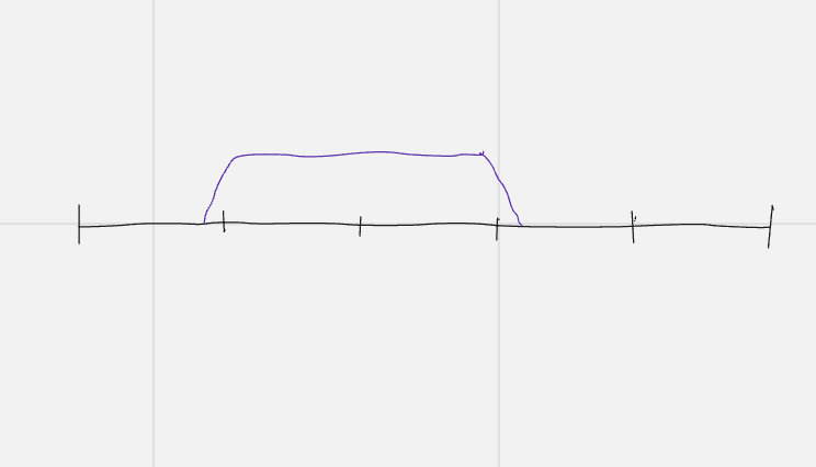
Now consider a general smooth manifold with a a collection of codimension one submanifolds. If is a smooth loop transverse to (a generic condition) then the pullback of a Thom form for is a Thom form for the intersection points , whose integral counts intersections between the image of and with signs. For example, if we take the Borromean rings as presented in Figure 1(a) and Thom forms for the Seifert surfaces in red and blue, the pullback will be Thom forms supported in the red and blue points on the left edge of the square in in Figure 1(b). If we consider the red surface alone, the pullback will look like the Thom form pictured in Figure 4(a).
3.1. First handlebody example
In Example 2.10 we saw that for wedges of spheres the zeroth Harrison cohomology is a cofree Lie coalgebra. We now calculate the simplest associated Hopf invariant (simplest aside from evaluation of cohomology).
Let denote a three-dimensional handlebody obtained by adding one-handles to a three-ball. Then is a -manifold with boundary and homotopy equivalent to a wedge . We consider the case . Label the two handles by and , and by abuse we use the same letters for the generators of represented by loops along their core disks. Let be a belt disk of the handle as in Figure 5, and let be a Thom form for of mass one. The form counts the (signed) number of times a closed loop winds around the handle , since if meets transversely,
Similarly define and for the handle .
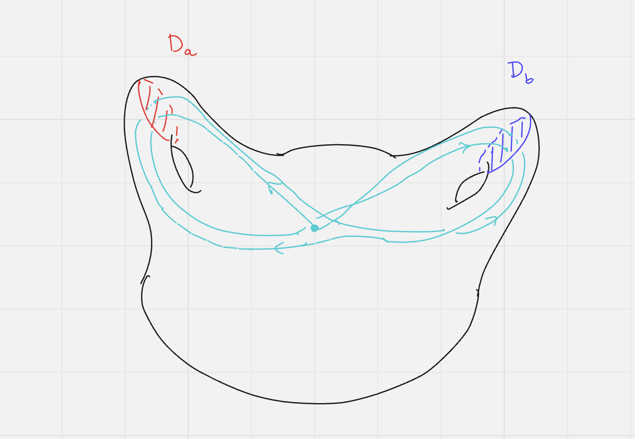
Consider the loop with shown in Figure 5. We calculate the Hopf invariant associated to on . With appropriate choices of parametrization and Thom forms, , where is shown in Figure 4(a), and we set , which is the time translate of by . Thus . Then recalling from Figure 4(b), the Harrison -cochain will have total differential
| (3) |
This implies that is homologous to in the Harrison complex of the circle – the latter is a form of mass one supported near . We conclude that , which is equal to .
A similar calculation shows that in general, if then we can pair ’s with ’s in the word , and is equal to the total number of ’s which occur between - pairs, counted with appropriate signs. This count can be seen as the linking number of the zero-manifolds and inside . Indeed, for any two submanifolds manifolds whose dimensions add to , Whitehead’s integral formula for the Hopf invariant [Whi47], namely , computes the linking number of and , where and are respective Thom forms. When the manifolds and are discrete, and when pulled back from a map representing a word the corresponding invariants are letter linking invariants, as we now show.
3.2. Equating topology and combinatorics of letter linking
In Section 1.2 we used simple combinatorics to define letter braiding functions on free groups. In Section 2.2 we defined Hopf invariants topologically. We now show that these coincide when considering fundamental groups of handlebodies and restricting to “good” symbols.
Let be a free group. We present it as the fundamental group of a handlebody , with handles corresponding to the , whose first cohomology is . Then is the vector space spanned by the indicator homomorphisms , respectively sending to and all other generators to .
The braiding symbols defining letter braiding functions in Section 1.2 map to our presentation of the Harrison homology of the handlebody, basically by changing ’s to ’s. Since the handlebody is formal and has cup trivial products, there is a canonical isomorphism . Therefore, the Hopf invariants of are represented by rooted trees decorated by homomorphisms , just as braiding symbols, and we can let be the map of vector spaces which sends a linear combination of braiding symbols to the class it represents in .
While letter braiding invariants of words and Hopf invariants of (free) groups are globally defined, they only agree with Hopf invariants in the following special setting.
Definition 3.1.
A letter braiding product is said to be a linking product when .
A word is an eigenword for a braiding symbol if all of the constituent braiding products in are linking products. The restriction of a letter braiding function to the subset of eigenwords is called a letter linking function.
The term “letter linking” arises as discussed at the end of Section 3.1. For example, we consider the indicator homomorphism on a word where the total count of ’s is zero. Pairing off the ’s, the values of record how many – pairs enclose a given letter of . If the total count of ’s is not zero then we do not have such “closed strings” connecting ’s and ’s, so the calculation involves “open strings”, hence the term letter braiding.
To relate letter linking to Hopf invariants consider a word of length , and let denote the map which represents in , for definiteness later say by traveling through the core of each handle at constant speed in time .
Theorem 3.2.
If is an eigenword for then
The first equality is by definition of letter braiding functions. We gave a first example of this in Section 3.1.
The rest of this section is devoted to proving this equality. We relate the two evaluations on by carefully choosing cochain representatives for , generalzing the constructions in Section 3.1. To do so is elementary but requires some language to specify the Harrison cochains which make equality apparent.
First, we define a family of Thom forms of belt disks. Fix a non-negative one-form with support on the interior of with total integral one. If is an interval, let denote the one-form which on is the pull-back of by the order-preserving linear homeomorphism of with and outside of is zero. On a handle let denote the pullback of along the projection to the interval.
To consider all possibilities for the placement of such forms on a handle, let be the set of -tuples of subintervals of . Explicitly, is in natural bijection with . (These sets also have a natural operadic structure, which contains the little one-disks as a sub-operad, but we will not use this fact.)
Braiding symbols are generated by homomorphisms under the braiding product. Consider linear combinations of such symbols and declare the braiding product to be bilinear. Then all letter braiding symbols are spanned by those where each is an indicator homomorphism for some . Let elements in this spanning set be called indicator symbols.
We now construct a cochain-level version of the map above which encodes the correspondance between braiding symbols and the Harrison cohomology of handlebodies.
Definition 3.3.
Let be a weight indicator symbol and . Define the realization to be the Harrison cochain represented by the same rooted tree (changing ’s to ’s), whose -th vertex is decorated by the form supported on the handle indexed by if the -th vertex of has indicator function .
Extend the realization linearly to all symbols to obtain a map .
In summary, we are realizing braiding symbols at the cochain level by linear combinations of Thom forms for belt disks which are supported on sets of intervals parametrized by . Below, we utilize a particular subset of such realizations.
Recall that the vertices of a rooted tree are partially ordered, with if is on the path from to the root (and the root a maximal element). Call a pair order compatible if whenever in the interval corresponding to is entirely to the left of the one corresponding to . We claim that an order-compatible realization pulls back to the circle along the map so that this pullback is homologous to a single form that matches the d-function combinatorially.
To make this precise, we say a form on the interval represents a d-function if it is supported on the interiors the sub-intervals and its mass on the -th sub-interval is . Clearly, the integral over of a form which represents a d-function is equal to the discrete integral over of that d-function. Thus Theorem 3.2 is an immediate corollary of the following.
Theorem 3.4.
Let is an eigenword for , and let be order compatible with . Then the pullback of the realization weight reduces to a form which represents .
Proof.
We will prove the following stronger statement by induction on weight. If is a sub-interval, let denote its image under the increasing linear homeomorphism if has , and the decreasing linear homeomorphism when . Then the pullback can be weight reduced to a form whose restriction to the interval has total mass and is supported on the interval , where is the interval corresponding to the root vertex.
In weight zero, no weight reduction is necessary. If is a homomorphism decorating the unique vertex in then the realization is the form restricting to each handle as some bump form with mass . Thus its pullback along the loop is indeed has a sum of bump forms with respective mass supported in the sub-interval . Note that if a letter in is the inverse of a generator then the loop travels through the handle backwards, mapping through the order reversing homeomorphism .
Proceeding by induction, consider a braiding product , suppressing decorating homomorphisms from the notation. Note that the eigenword assumption means in particular that is an eigenword for both and .
Let denote the sub-interval corresponding to the root of . Then by the inductive hypothesis the pullback can be weight reduced to a form on with support in and total mass . The eigenword assumption implies that this mass is zero. Therefore has an anti-derivative as a form (as in Figure 4(b)), which is constant outside of the intervals and whose constant values given by the partial sums of the masses of . Similarly, can be weight reduced to a form supported on the intervals for .
It follows that the entire pullback can be weight reduced to the form . This product is immediately seen to have support contained in that of , as claimed. Furthermore, the intervals are disjoint from , so the form is locally constant on the support of .
Finally, we calculate the mass of the weight reduced form on . Since was chosen to be order compatible with , the interval is entirely to the left of . After applying the homeomorphism , we see that is still to the left of . In this case, the (constant) value of on is the partial sum of up to and including the -th value. However, if then the orientation of is reversed so that is on the right of , which implies that the value of on is the partial sum not including the -th value. This is exactly the form of the d-function multiplying the d-function , as claimed. ∎
3.3. Configuration braiding of trees and words
Rooted trees give an alternate way to view the evaluation of letter braiding functions from Section 1.2 akin to the configuration pairing of [SW11]. Let be a word in and let be a rooted tree with vertices labeled by homomorphisms . Braiding symbols are equivalent to (sums of) such rooted trees by formally converting to .
Definition 3.5.
A configuration of is a weakly decreasing function with respect to the partial ordering on induced by the root. That is, the root is a maximum elements and if the unique monotone path from the root to passes through .
A configuration is proper with respect to if is strictly decreasing at whenever . That is, the inverse image must not contain comparable vertices (, with either or ).
The associated pairing is where is the label of vertex and .
The restriction to proper configurations is necessary to account for the effect of when computing in Definition 1.5.
It is instructive to compare evaluated on versus . On there is only one proper configuration , leading to a value of . On there are three proper configurations , , and , leading to a value of .
Proposition 3.6.
Letter braiding functions count proper configurations of in .
Example 3.7.
Consider evaluating on the word . Only three configurations yield nonzero pairings.
-
•
, contributing
-
•
, contributing
-
•
, contributing
The sum of these is , recovering .
4. Structural theorems
We establish the main formal theorems governing Hopf invariants, starting with the fact that the Hopf pairing establishes a Lie coalgebraic duality, then giving a lifting theorem which relates Hopf invariants of two complexes and their one skeleton, and finally we establish universality using the lifting theorem.
4.1. Lie pairing
We use the standard approach to Lie (co)algebras through (co)associative algebras and Hopf algebras. Fundamental group invariants in (co)associative setting were developed by Chen.
We first recall the standard presentation of the Malcev Lie algebra. For a group let be the completion of its group ring at the ideal generated by elements of the form for . For example, the power series
converges in . This ring is naturally a Hopf algebra, with product and coproduct for all group elements . Recall that primitives in a Hopf algebra form a Lie algebra.
Definition 4.1.
The Malcev Lie algebra of the group is the Lie algebra of primitive elements in .
Quillen showed in [Qui69] that this is a complete filtered Lie algebra, topologically generated by elements of the form for . Moreover, he showed that the logarithm function preserves filtrations when and are filtered by their respective lower central series, inducing an isomorphism of associated graded vector spaces after tensoring with . (For a thorough treatment see Appendix A in [Qui69], and Section 2 of [Mas12].) Recall the notion of a Lie pairing from Definition 1.1.
Theorem 4.2 (Theorem 1.2, Lie pairing).
Hopf invariants extend uniquely to a Lie pairing, with
for every and group element .
Uniqueness of such a pairing will follow from the stated bracket-cobracket duality, which forces the pairing to be continuous with respect to the filtration by commutator depth, while is topologically generated by the . We call the resulting pairing the Hopf pairing.
Recall that the Baker-Campbell-Hausdorff series is a formal power series in a completed Lie algebra satisfying
This series governs values of Hopf invariants.
Corollary 4.3 (Aydin’s Formula).
Hopf invariants of products in are given by the Baker-Campbell-Hausdorff formula:
Proof.
We apply the defining property of the BCH series to taking and . ∎
Remark 4.4.
The second author originally found a proof of Corollary 4.3 with finite generation hypotheses using the theory of -algebras. Briefly, a -algebra is a graded vector space with a coderivation on which squares to zero, defining a Harrison complex. Morphisms are just maps on Harrison complexes.
In [BFMT20] the authors show that the simplicial cochains on a simplicial set have a structure extending cup product which is quasi-isomorphic to the PL de Rham cochains on that simplicial set. In the case of the one-simplex this is dual to the Lawrence-Sullivan interval.
The “universal product” on fundamental groups is given by a collapse map . The second author made explicit calculations in this model to see that weight reduction in the Harrison complex leads to Baker-Campbell-Hausdorff product. He used this to achieve our first proof of the Lifting Criterion below, in the finitely generated setting.
Proof of Theorem 4.2.
Let be the de Rham forms (smooth or piecewise linear) for and consider a loop . We consider the interplay between the coassociative and coLie bar constructions
Chen defined an invariant of loops using the iterated integral. If is a loop, are a -forms and then
Chen’s invariant gives a linear map which extends to a bilinear pairing with the group ring . Letting denote the reduced coproduct of , Chen proves in [Che71, Eq. (1.6.1)] that
from which it follows that weight Bar cocycles vanish on the -th power of the augmentation ideal in . Thus the pairing extends to the completion . Define a pairing on by restriction to primitive elements, so if is primitive, set
where is any lift of to the coassociative Bar complex, which exists by Barr’s splitting [Bar68]. To see that this is independent of the choice of lift , recall that under Chen’s pairing the shuffle product on the Bar complex is dual to the group ring coproduct [Che71, Eq. (1.5.1)] from which it follows that nontrivial shuffles must vanish on primitive elements. Since the Harrison complex is the quotient of the coassociative bar complex by nontrivial shuffles, the pairing on primitives descends to Harrison homology.
Bracket-cobracket duality of this pairing follows quickly from Chen’s product-coproduct duality,
Vanishing of weight cocycles on -fold nested commutators follows immediately from this identity.
It remains to show that the pairing agrees with the Hopf pairing, by weight reduction on the Harrison complex of the circle. By work of Gugenheim [Gug77], Chen’s iterated integrals extend to natural isomorphisms between the top two rows of the commutative diagram
Chen’s invariant is the dashed arrow (this holds in all higher dimensional as well). Here, the surjection between the bottom two rows is Harrison’s quotient by shuffles.
Letting denote the dashed arrow, observe that it is the corestriction onto the cogenerator of the cofree coalgebra . Since Gugenheim’s maps between the top two rows are coalgebra homomorphisms, the image of in is
On the other hand, the map denoted by is the corestriction of the inverse to Gugenheim’s isomorphism, which is computed in [BS16, Proposition 1.7] (where both and are denoted by ) to be
With this, the image of in the bottom-right corner is seen to be
This shows that
for all . ∎
4.2. The lifting criterion
We relate the Harrison cohomology of a two-dimensional CW-complex to that of its one-skeleton. We use this criterion in the next two sections to prove the fundamental theorem that the Hopf pairing is a universal Lie coalgebraic extension of homomorphisms from a group to the rational numbers and to extend the theory of letter linking invariants to general groups.
For any simplicial set let denote the commutative differential graded algebra of PL differential forms on . Let be a two-dimensional complex with one-skeleton . Then is built by attaching -cells along maps for some set , and its fundamental group is the free group modulo the images in of the maps which by abuse we also call .
As discussed in Example 2.10 the zeroth Harrison cochomology of a wedge of circles is just the cofree Lie coalgebra on the linear dual . Our goal is to understand the map induced by inclusion of the one-skeleton , which by the following also yields a calculation of the zeroth Harrison cohomology of .
Proposition 4.5.
The map is injective.
Proof.
As shown in Remark 2.14, there are no differntials in to degree zero for the Harrison spectral sequence of any connected space. So zeroth Harrison cohomology includes in the -page. As is injective on first cohomology, it is also injective in total degree zero on this -page. But the spectral sequence collapses for a wedge of circles. So is a composite of injective maps. ∎
Definition 4.6.
Let denote the maximal sub-Lie coalgebra of whose Hopf invariants vanish on relations.
Theorem 4.7 (Lifting Criterion).
The image of is .
Informally, a Harrison cocycle lifts if and only if it and all of its cobrackets vanish on relations. The image of vanishing on relations is immediate, since by naturality the Hopf pairing can be computed on , in which case the lift of is null-homotopic. We will see examples below for which the closure under cobracket, whose necessity is also immediate, excludes some classes which vanish on all relations.
We analyze at the level of Harrison complexes, letting denote the collection of -closed elements. Let be the maximal sub-coalgebra whose Hopf invariants all vanish on the attaching maps. Thus restriction to the -skeleton gives a commutative diagram
| (4) |
The Lifting Criterion of Theorem 4.7 follows immediately from the following.
Lemma 4.8 (Lifting Lemma).
There exists a section which is a Lie coalgebra homomorphism.
The proof of this claim is the most technical aspect of our work. The key to our argument is to relate Hopf invariants of attaching maps to the Harrison complex of the attached disks.
Recall that Harrison cochains of weight zero in are simply elements in . In text below we will abusively write for both a weight zero element of as well as the underlying form in .
Lemma 4.9 (Circles and Disks).
Consider , the inclusion map of the boundary. Every Harrison cocycle is realized as a pullback from the disc for some cochain such that:
-
(1)
has weight ;
-
(2)
The -form is supported on the interior of ;
-
(3)
.
The integral on the left of (3) is the ordinary integration of a -form on the disc, while the integral on the right is evaluation defined in Proposition 2.11. An illustration of (3) is discussed in Section 5.4.
Proof.
The map is a surjection, so the induced map on Harrison complexes is as well. Define to be the kernel of and write for the cohomology of the resulting complex. The long exact sequence of relative Harrison cohomology reads
Homotopy invariance implies , so the connecting homomorphism is an isomorphism.
Let . The connecting homomorphism is defined by lifting and then applying , namely . The connecting homomorphism thus respects filtration by weight, since lifting and do. As is supported in (spanned by) weight zero, so is . We can thus choose an such that has weight zero. Let . Since (every summand of contains at least one form that vanishes on ), the cochain itself restricts to , and as desired has coboundary in weight zero, proving statement (1).
To prove statement (3), we first apply Proposition 2.11 to obtain an of weight zero. Extending to the interior of the disc results in a form such that
where the first equality is by Stokes’ Theorem. So it suffices to show that for some relative -form .
Observe that both and represent the element and they therefore differ by some for , possibly of positive weight. If we can show that where and has weight zero, then
as desired.
To see we can weight reduce , suppose it has weight and let be its summand of weight . The vertical component of must vanish on since this is the weight term of which is only supported in weight zero. So is a -cocycle in the complex equipped with only the internal (vertical) differential. But both and have no vertical cohomology in degree zero in this weight by the Künneth Theorem, so neither does . Thus is the image under the vertical differential of some . It follows that has weight and still cobounds the difference of . Performing this weight reduction iteratively lets us subtract coboundaries from until the result has weight zero, completing the proof.
∎
With these facts in place we can proceed to proving the Lifting Lemma.
Proof of Lemma 4.8.
Extend the diagram from Equation (4) to the right using maps projecting onto cogenerators:
We define the desired section by climbing the weight filtration inherited from . To start, choose splittings so that . Furthermore, pick an arbitrary section by extending the domain of definition of differential forms to the interiors of the -cells in . By construction, is a section of the restriction map .
We build by constructing a coalgebra homomorphism landing in -closed elements. Since is cofreely cogenerated by , such a map must be the cofree coextension of some . We use the weight filtration on to define . Begin with
and let be the cofree extension to a homomorphism into . The induced homomorphism is indeed a section of the restriction , however it does not necessarily send to -closed elements. We perform a modification at each step to get maps whose cofree extensions to homomorphisms map to -closed elements. We first consider this modification in detail to get from . Given , we calculate
since in we have . Because cobrackets are injective in positive weight by Proposition 2.7 we deduce that has weight zero. By assumption, has vanishing Hopf invariants on all so by the Circles and Disks Lemma 4.9,
where is the two-disk attached by . By the the relative cohomology long exact sequence for and its one-skeleton, any cohomology class which evaluates to zero on all must cobound. Thus the -form has a cobounding such that .
Pick a basis and define by linearly extending
on and elsewhere. Since the forms restrict to zero on , we have not changed images after restriction , and is now -closed by construction.
The general case is almost identical. Given extending to with the property that sends to -closed elements, we first note that must have weight zero, again by applying injectivity of cobracket, now using the fact that tensor factors of have weight but of such terms is zero. That is,
Thus we can apply the Circles and Disks Lemma as before to find coboundings of and use these to define such that and of is now -closed. ∎
4.3. Letter linking algorithms
There is a simple, quick algorithm which can be used to evaluate letter braiding functions, from Section 1.2, on words. Rather than being recursive, a single pass across the word suffices. To evaluate we store homogeneous symbols as their corresponding tree where each node contains a d-function and two variables and , initially set to 0. Evaluation is computed letter-by-letter in the word, depth-first (away from the root) in the symbol. For each letter and node , the and values are updated as follows.
-
•
First is incremented by the current value, and is reset to 0.
-
•
Next the sum of all parents’ -values is multiplied by the d-word value at the given letter .
-
•
If letter is an inverse then this product is added to . Otherwise it is added to .
After evaluating over all nodes at all letters, the value of the braiding symbol on the given word is the sum at the root node of the invariant. During the course of computation, at letter of the word and node of the braiding symbol, where is the subsymbol supported above node . Thus the sequence of values of give the d-word .
It is substantially more involved to generate letter braiding functions which are well-defined on a group . Applying the Lifting Criterion from Section 4.2 we know these are invariants on whose iterated cobrackets all vanish on the relations in . While the vanishing of iterated cobrackets on relations seems like a large set of conditions to check, it leads to fairly simple algorithms for generating letter linking invariants up to a fixed weight.
At an abstract level, start in weight zero, where we recall that the indicator homomorphisms are a basis for . These evaluate on relations by counting (signed) occurrences of letters. Thus vanishing on a given relation imposes a linear condition on the coefficients of . Calculating the kernel of all such conditions yields , the weight zero letter linking invariants for .
In higher weights, the vanishing of cobrackets on relations comes into play. Write for the vector space of weight letter linking invariants of which lift to in the sense of Theorem 4.7. If is known, then we may compute the cobracket compatible vector subspace as the preimage of the vector space under the cobracket (implicitly identifying ). The next set of invariants, , is the vector subspace of which vanishes on all relations, as calculated by the fast evaluation algorithm above. Note that contains (as well as all of ), so .
Implementations of this depend on choices for how these vector spaces are defined and computed. The second author created one SageMath implementation [Ozb23], using BCH expansions and his Formula (Corollary 4.3) to check vanishing on relations. Given a word in the set of generators , let be the BCH expansion of , extending the BCH product:
Write for the truncation of to include only weight terms, computing in the free -step nilpotent Lie algebra, . The code works in using an previous implementation of Hall basis for . If is a Hall basis element, then is the coefficient of in the BCH expansion of . Thus, written in terms of a Hall basis, is the matrix of coefficients of the BCH expansion through weight .
Using SageMath functions for Lie algebras and vector spaces, the code works as follows.
-
(1)
Make the vector space .
-
(2)
Construct the linear transformation evaluating on relations .
-
(3)
Get the kernel of . This is , the weight zero letter linking invariants.
-
(4)
Loop over the following steps.
-
(a)
Expand the previous vector space from to by including the next weight of (dual) Hall basis elements.
-
(b)
Make vector space
-
(c)
Make the cobracket linear transformation
as the transpose of the -nilpotent bracket transformation
-
(d)
Calculate the preimage of the vector subspace . This is .
-
(e)
Make the linear transformation
-
(f)
Calculate the kernel of restricted to . This is .
-
(a)
There are many possible optimizations to make. We are interested in an implementation which is more fully Lie coalgebraic, rather than relying on existing implementations of Hall bases and working through duality. Such an approach could lead to evaluation through the “one-pass” algorithm outlined at the beginning of this section, rather than more intensive Baker-Campbell-Hausdorff series.
4.4. The Fundamental Theorem
Theorem 4.10 (Universality statement of Theorem 1.2).
The Hopf pairing of with the Malcev Lie algebra of is a a universal Lie pairing.
The Lifting Criterion immediately gives a way to deduce this theorem for general groups from the free case. We start with the following refinement of the calculation in Example 2.10.
Lemma 4.11.
Let be a wedge of circles indexed by a set and let denote the inclusion map of the circles with label . Under the canonical isomorphism we have
for every homogeneous expression .
Proof.
A commutative cochain model for a wedge of circles is the square-zero algebra , whose Harrison complex is concentrated in degree . The circle inclusion is modeled at the cochain level by the algebra homomorphism
sending a function to its evaluation . This pullback induces a weight preserving map on Harrison complexes . But since the target is one dimensional and concentrated in weight zero, it follows that all positive weight homogeneous elements are sent to . ∎
Proof of universality (Theorem 4.10).
First, if is a wedge of circles indexed by a set , then on the one hand the free group on basis and on the other hand its Harrison cohomology is isomorphic to .
To see that the Hopf pairing is universal, let be any Lie pairing. Then the map given by
extends uniquely to a Lie coalgebra homomorphism by cofreeness of the target. We show
all and . First, consider for a generator . The previous lemma shows that the Hopf pairing vanishes on homogeneous elements of positive weight in , so we have
by definition of .
Now, suppose by induction that the equality holds for elements . Then
since both pairings are Lie pairings. This shows that equality holds on the Lie algebra generated by for . Lastly, suppose has weight . The Baker–Campbell–Haudorff relation shows that every coincides with an element from the latter Lie subalgebra up to -fold nested brackets, so the two elements have equal pairings with . This completes the proof in the case that is a wedge of circles.
Now, suppose is a two-complex with fundamental group and one-skeleton a wedge of circles indexed by a set . The inclusion induces a presentation with kernel normally generated by the attaching maps of -cells .
If is a Lie pairing, then it induces a Lie pairing with by precomposition with . Thus, by the already proved case of a wedge of circles there exists a unique Lie coalgebra homomorphism pulling back the Hopf pairing to .
But, since every relation is killed by the projection , the image of pairs trivially with all relations. That is, the image is contained in the subcoalgebra from Definition 4.6. Since the lifting criterion in Theorem 4.7 shows that the pullback is an isomorphism onto , and since is a coalgebra homomorphism that preserves the Hopf pairing, we get a map
pulling back the Hopf pairing to . Uniqueness of this map follows from the fact that after composition with we must get back the uniquely determined map , but is injective. ∎
In the course of proof we obtain an independent calculation that the Malcev Lie algebra of a free group is a free Lie algebra. Moreover, as a corollary of this, Theorem 3.2, and Quillen’s theorem comparing lower central series and Malcev Lie algebras, we get a topological proof of the main theorem of [MS22], that letter-linking invariants obstruct the lower central series of free groups. We can now prove our main combinatorial application.
Proof of Theorem 1.10.
The theorem is phrased in terms of braiding functions, so let us first translate the statement into one regarding Hopf invariants. From Section 3.2 we know that the combinatorially defined braiding functions agree with Hopf invariants of some realization form. Moreover, braiding functions clearly span all Hopf invariants for the free group, as seen e.g. by the fact that the Harrison spectral sequence for the handlebody collapses to . Finally, by the lifting criterion in Theorem 4.7, a Hopf invariant of descends to if and only if it belongs to the Lie dual of . So it suffices to prove that the image of in has a power that is a product of -fold nested commutators if and only if all weight elements in the Lie dual of vanish on .
Let denote the lower central of , that is and , and analogously for . Quillen proved [Qui68, Equation (1.5)] that the natural map induces an isomorphism
It follows that some power of lies in if and only if its logarithm lies in .
It remains to show that if is a Lie dual of then is exactly the kernel of the evaluation on the weight elements of . The fact that such evaluations are trivial follows immediately from the bracket-cobracket duality: if has weight then its -fold iterated cobracket is zero, which by duality implies vanishing on -fold nested commutators.
For the converse, suppose is not in . Then it represents a nontrivial element in the finite dimensional Lie algebra . Its linear dual is a Lie coalgebra whose elements all vanish after iterations of the cobracket, with an obvious pairing with . Furthermore, by linear duality it contains a functional that does not vanish on . By the universal property of the Lie dual, there exists a coalgebra map that pulls back the Lie pairing. But then
exhibiting as an element of weight on which does not vanish. ∎
5. Examples
5.1. Orientable surfaces and our favorite little two-complex
The torus provides a counterpoint to the free group setting. The standard model for the torus is a differential graded commutative algebra on generators and in degree one, with non-trivial product . The Harrison complex for this algebra has homology only given by and themselves in weight zero, and of course these span the dual of the group. All other cochains in degree zero have a basis whose boundaries are linearly independent. That higher Hopf invariants are trivial in the abelian setting makes sense as they arise from derived abelianization.
Surfaces provide an opportunity to see both geometry and algebra. We use Thom classes of curves, as developed in Appendix B.1, but in this case without a need to thicken a two-complex to obtain a manifold. We picture the genus two case below, with “dual” curves , , and and choosing associated Thom forms of the same name as generators of first cohomology. While the products of pairs of generators are equal in cohomology, we have at the cochain level.
![[Uncaptioned image]](/html/2403.20264/assets/Figures/surface.png)
In weight zero, Harrison cocycles are and . In weight one, and similar involving pairs of cochains with zero product at the cochain level are all cocycles. Following the analysis of Section 3.1, the Hopf invariant associated to would be the count of when a loop crosses curve in between crossings with opposite signs of .
Another Harrison cocycle is . The corresponding counting invariant would be the sum of the count (with signs) of occurrences where a curve crosses in between crossings with , occurrences of -crossings in between ’s, and crossings with . A simple homotopy of a curve “from left to right” across the octagon would result in this count to have contribution from different parts of the sum.
If we restrict loops to the one-skeleton, and simple homotopies across the 2-cell, we obtain the standard generators and relations presentation of this group. We see that because the number of ’s between pairs and that of ’s between pairs can both change individually, but their difference will be invariant. This difference, represented by the braiding symbol , is the letter-linking representative of the Hopf invariant associated to . From this algebraic perspective, there is no evidence of a “correction curve” , which topologically is disjoint from the one-skeleton. In general, model the cochains of the genus-two surface by the commutative differential graded algebra generated by in degree one with all products zero except . We define the standard involution on this algebra to be the one switching with and with . To calculate the homology of we find a suitable basis for , namely graphs whose symbols do not contain the following as sub-symbols:
as well as subgraphs obtained from these by applying the standard involution. We call such graphs admissible. That admissible graphs span is an immediate application of the Arnold identity. In such graphs, any edge connecting an to is isolated, as are those connecting a to a . Moreover, by eliminating graphs such as , this isolation remains when we apply the standard involution to an edge. Calculation in such an admissible basis is immediate, with cocycles given by linear combinations of terms obtained from each admissible graph with edges of the form or by applying the standard involution to those edges.
This calculation speaks to the strength of the Eil-graph approach to Lie coalgebras, as we think it would be difficult to find a suitable basis through bar elements (long graphs) modulo shuffles. It also speaks to the clarity that the graphical approach gives rather than just working with symbols, as for example is a well-defined letter linking invariant but is not.
Higher genus surfaces behave similarly. Another similar example is for the group , the fundamental group of a two-complex homeomorphic to a cylinder with a pair of points on its boundary identified. It is homotopy equivalent to a wedge of two circles, so is isomorphic to a free group on two generators, say and . Let , and be indicator Thom cochains associated to curves and a compatible Thom cochain of a point as pictured below.
![[Uncaptioned image]](/html/2403.20264/assets/Figures/favoritelittle.png)
In weight zero and generate the cohomology of . In weight one is a Harrison cocycle. It pulls back to a cocycle of the same name on the one-skeleton, to which we associate the letter linking invariant . In group theory, the count of ’s between collections of cancelling ’s and ’s can change under the relation, increasing by one, but as it does so does the number of ’s. One could also choose as a representative, differing by which is a cocyle of lower weight.
In higher weights the story is conceptually simple but the combinatorics can be complicated. Consider the cofree Lie coalgebra generated by . The Hopf invariants for must be isomorphic to this algebra. Accordingly, we claim that any corresponding cochain can be completed to a cocycle. This is because the Harrison differential introduces products, realized by Thom forms of points, but these can be cobounded by cochains in for which one replaces such points by parallel copies of or . In some cases this replacement results in further products and thus correction terms needed in lower weights, so the correspondence between Hopf invariants for and those for the free group on two generators is not tautological.
5.2. Milnor invariants for Borromean rings
Application to Milnor invariants has been a prime motivation, as first discussed in Section 1.3. We return to these in light of our general theory.
Consider the Borromean rings, with two presentations given below.
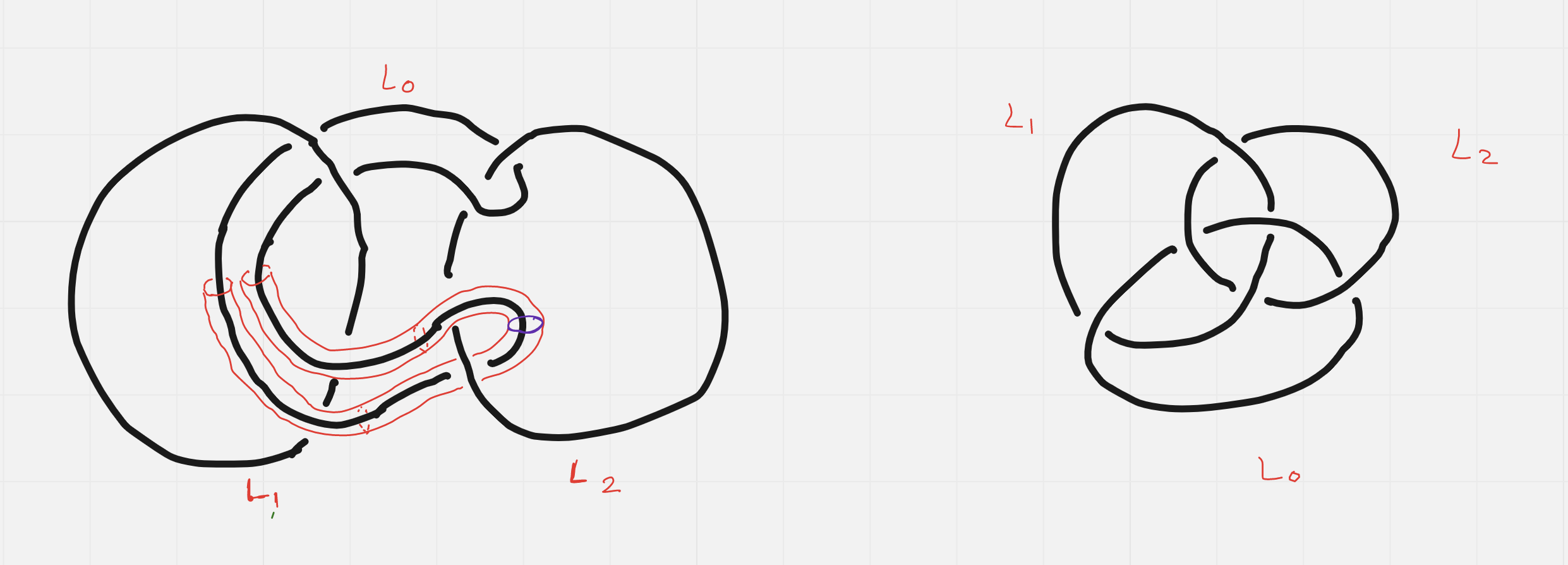
We consider the component as defining an element in the fundamental group of the complement of the other components, . For brevity of discussion we ignore basepoints and orientations. We again use Thom forms (Appendix B.1).
In the first presentation we assume and are planar circles, and let be the planar disk which bounds and similarly for . Because these are disjoint, the associated Thom forms and , which form a basis for first cohomology of , define a Harrison cocycle . With appropriate parametrizations, pull-back of this to is a Harrison cocycle on the circle from Section 3.1, pulled back from a commutator on a handlebody. Thus the Hopf invariant will be one, counts the intersections of with which occur between its intersections with . On this evaluates as .
Following Cochran [Coc90] we make an alternate choice for the first Seifert surface by removing small disks at the intersection points of with and replacing them by a cylinder which is a unit normal sphere to on one side, as pictured. There are two things which change when using in place of . First, does not intersect . Secondly, is not a Harrison cocycle on , since is a small circle around an intersection point of with .
To complete it we can choose any surface which cobounds this circle – a small disk around , or its complement in , or for example a cobordism between this circle and – and then with appropriate modifications its Thom form will complete a Harrison cocycle . Whatever choice for will yield the same value of when evaluated on , as this will be the linking number of with the circle . Indeed, Cochran’s perspective is that this form of the Milnor invariant is realized as a “derivative” linking invariant. We can also modify to eliminate its intersections , but by “nesting” the cylinder added for that purpose with the existing one, the intersection of and will be the same as that of and , so the analysis from there will coincide.
Next, we work with a standard diagrammatic presentation, given on the right of Figure 6. Following Seifert’s original algorithm suppose each component to be planar except on some arbitrarily small intervals near some crossings, with the plane lower than that of which is in turn lower than that of . Thus where over-crosses of it must “rise up,” which can be assumed to happen in an arbitrarily small neighborhood of the crossing.
We choose “mostly flat” Seifert surfaces and which are disjoint except near these crossings, where they intersect because goes from being under to over it. The intersections are small curves with one endpoint on and the other on , which in projection are arbitrarily close to the crossing points. Thus the associated Thom forms and have wedge product which is a Thom form for the union of these two curves.
To complete a Harrison cocycle we find a cobounding surface for this intersection. Once again using the projection as faithfully as possible, we can take the closed loop consisting of these two curves along with a portion between these crossings, and a portion of between them, say the shorter portions for definiteness. We cobound this closed loop with a disk which agrees with except near the crossings and near the part of the boundary where it must “fall downward”. With these new definitions, our Harrison cocycle has the same formula as above.
By construction, since is generally below all of this, the intersection of with these surfaces would occur only at crossings of over or . But only crosses under . Thus the pullback of to the circle parametrizing will be zero, since the pullback of is zero. The term evaluates as an intersection count of with , or equivalently a linking number with the “derived” link component . There is one such intersection point namely near the -over- crossing which is on the boundary of .
Thus, in the setting of links, one can work closely from a diagram, or look to minimize some types of intersections, or to make use of some geometric structure, giving different approaches to the same set of invariants. As discussed in Section 1.4.3, part I, we plan to develop this further in a sequel.
5.3. Beyond letter linking
Letter linking is by definition an obstruction theory, as the invariants require vanishing to be defined. But Proposition 2.11 shows that all Harrison cocycles on the circle can be weight reduced. Following this through produces surprisingly rich combinatorics, and also motivated the first author to take weight reduction seriously on the classical bar complex [Gad23].
We recall the notation of Section 3.1 and calculate the Hopf pairing of the cocycle and the word in the free group as the fundamental group of the handlebody . For definiteness, parametrize so that the curve defining passes through the at and at . Then pulls back to .
Neither entry of this Harrison cochain cobounds. But we can still weight reduce by taking advantage of the fact that by definition any weight one cochain with repeated entries is zero. Let
so that . Then
As the term is zero, this exhibits a weight reduction of our orignial pullback to the weight zero cochain . This then can be evaluated to , as predicted by Aydin’s Formula, Corollary 4.3.
5.4. Commutators and Massey products
Our theory extends the time-honored connection between vanishing of Massey products and homomorphisms out from the fundamental group. Consider . We again realize as the fundamental group of a two-complex with one cell, and employ Thom cochains for dual curves as pictured.
![[Uncaptioned image]](/html/2403.20264/assets/Figures/masseycommutator.png)
As discussed in Appendix B.3, the cochains , and map to corresponding cocycles on the -skeleton, and they are themselves cocycle lifts. Moreover lifts to , lifts to with no correction term needed and similarly for . The Harrison cochain however does not complete to a cocycle. It does partially complete to , whose total differential is in weight zero, but that differential is a Thom cochain of the intersection point of and , which does not cobound an available cochain in weight zero of the Harrison complex.
The value of this total differential on the fundamental class of two-complex is one, as there is one intersection point, which coincides with the value of the letter linking invariant associated to on the defining relation . Such an equality in general is proven in Lemma 4.9. We can see in this example how the process of completing curves to define Thom forms and intersecting them parallels the cobounding and intersecting of letter linking. For example, the curves each are “parallel to” intervals between pairs on the boundary, and their intersections with curves can be traced back to occurrences of ’s between those pairs. In other words, if we restrict the extensions of these curves from the boundary to the two-disk to lie in an epsilon neighborhood of the boundary, their combinatorics matches that of letter linking invariants. We originally pursued proofs of the lifting Theorem 4.7 which codified this.
This weight zero differential is also immediately recognizable as a Massey product, namely , in the cohomology of this two-complex. Indeed, as we discuss in Remark 2.14 and Section A.1, Massey products define differentials into the weight zero column in the Harrison spectral sequence. Massey products then tautologically obstruct lifting from the Harrison complex of the one-skeleton of a CW-complex. But instead of formulation in terms of Massey products, Lie coalgebraic formalism is the appropriate language for our structural theorems, in particular the clean formulation of Theorem 4.7.
5.5. Pure braid groups
We apply machinery of the Harrison complex to the space intimately tied to its definition. Namely, the space of configurations of distinct labelled points in the plane is a manifold whose fundamental group is the pure braid group and whose st cohomology group is isomorphic to (up to “signs”). This Harrison complex consists of Eil-graphs decorated by Eil-graphs, though for sanity we use the more traditional presentation of cohomology as generated by modulo the Arnold identity.
At the cochain level be the Thom form associated to the submanifold defined by having point over point , so is a positive scalar multiple of . We (co)orient this submanifold so that the “positive” normal direction is when point is slightly to the left. Then for example the wedge product will be a Thom form for the submanifold where point is above which is above .
Consider the codimension one submanifold with boundary defined by having point over point and point with -coordinate which is greater than or equal to the shared -coordinate of points and . The boundary is when the -coordinate of is equal to that -coordinate. There are naturally three components, depending on whether point is over , in between, or below . Thus cobounds the Arnold identity:
Immediately we can construct a Harrison cocycle
By bracket-cobracket compatibility, it pairs non-trivially on the commutator (This equality of commutators is the defining relation of a Drinfeld-Kohno Lie algebra .)
The corresponding Hopf invariant will have four terms, which we interpret in terms of standard braid diagrams. The term counts -over- crossings, but only those for which strand is to the right. Weight reduction on will yield a count for example of between canceling pairs . Geometrically, in this setting strands and are not linked, but strand ’s being counted are “coming between them” and so possibly linking.
5.6. An infinite example
Consider the group generated by and with for all . Such a group is the fundamental group of a countable union of genus one surfaces with one boundary component, with all such boundary components identified with each other. We consider closed dual curves as in Section 5.1 (with the genus two surface being the version of this infinite complex), so that intersects in a point and otherwise these curves are disjoint.
Possibly infinite unions of such curves are define proper submanifolds of the thickening of this complex and thus Thom cochains. These realize the first cohomology group, which is an infinite product rather than sum.
Harrison cocycles , for for any , are a dual basis to the corresponding . But is detected by , which also pairs with any . This Harrison cocycle is not a finite sum of more basic such. Key here is that the first cohomology is already a direct product so infinite sums can be “embedded” in the standard Harrison complex.
5.7. Beyond residual nilpotence using the product totalization
First recall from Definition 2.8 that the Harrison complex is defined as the standard total complex of a bicomplex . There is an alternative totalization of a complex defined using direct product in each total degree, from which we get a variant of our theory.
Definition 5.1.
Define the completed Harrison complex as the direct product totalization
We will not fully develop a theory based on the completed Harrison complex here, but do give an example to show that it detects phenomena beyond the residually nilpotent setting, which has been a universal limitation for group theory through computational algebraic topology.
Consider the group generated by , with relations . Thus any is in the intersection of all commutator subgroups. We realize this as the fundamental group of the quotient of the union , where each is a genus one surfaces with one boundary component, by identifying the boundary of with the longitude of , as in the theory of gropes. Explicitly, we build this two-complex as a union of pentagons as pictured on the left below. By abuse we use to decorate edges, which under identifications are loops, though for the fundamental group paths from the basepoint must be given.
![[Uncaptioned image]](/html/2403.20264/assets/Figures/pentagons.png)
We use Thom cochains for a fattened four-manifold homotopy equivalent to this two-complex as in Appendix B.1. Though we normally prefer to use capitalized versions of generator names for dual cochains, for clarity let be the dual curve to in , a segment between midpoints of the edges in the pentagon preimage of , and similarly for , as pictured on the right above. Let be the segment between the midpoint of and the intersection point of and .
With appropriate choices of Thom forms, the infinite sum
will be a cocycle in the product Harrison complex which will evaluate non-trivially on . Algebraically, the corresponding letter linking count is “sensitive to infinitely many possible subwords”, but is well defined since only finitely many of them could occur in a word.
This infinitary construction echos other recent developments in non-simply connected homotopy theory. As discussed in Section 1.4.3, Rivera–Zeinalian [RZ21] and Rivera–Medina [MMR23] show that the cobar construction on singular chains of a space faithfully encodes the fundamental group, but in a way that does not lend itself to calculation because of lack of quasi-isomorphism invariance and convergent spectral sequences. The completed Harrison complex might serve as a bridge to theories such as these, with some ability for calculations by hand while being able to see beyond traditional nilpotence restrictions.
Appendix A Bar and Harrison complexes
A.1. Basics and connection with Sullivan models
Bar constructions are standard in homological algebra of modules, but are less familiar in the context of algebras, for functors such as indecomposibles. We share this perspective, which is key to understanding the Harrison complex and its relationship to the well-known Sullivan models of rational homotopy theory (from which we have borrowed our title).
Definition A.1.
Let , be an associative differential graded algebra, with augmentation ideal .
The classical Bar complex denoted is the second-quadrant bicomplex for which the th column is , with elements denoted . The vertical differential, on , is , extended by the Leibniz rule (with Koszul signs reflecting a desuspension of every tensor factor of ). The horizontal differential is the alternating sum of on consecutive factors, sending
The spectral sequence of a bicomplex applies to give the Bar spectral sequence, a standard organizational tool. Taking homology with respect to the vertical differential first, the spectral sequence has given by . The first differential reflects product structure, for example leaving the indecomposibles of in the zero column at the -page. Higher differentials reflect Massey products, and indeed this can be taken as a definition of Massey products. For example, if and then
will have total Bar differential , which represents the Massey product . This will give rise to a non-zero -differential in the Bar spectral sequence if and only if the Massey product is non-zero modulo standard indeterminacy.
The classical Bar complex arises in topology in a few ways. If is a group ring, it computes group homology with trivial coefficients. If is the cochain algebra of a simply connected space, it models cochains on the loop space. There are many perspectives for this latter fact, with two relevant for the present theory. One is that if are Thom forms as in Appendix B.1 or geometric cochains, then essentially counts intersections of a loop (within a family of loops defining a smooth chain on the loopspace) with the , in order. If has boundary, this count can change through a homotopy of a loop or more generally a homology of a cycle of such loops. The count can also change if the intersect, as we saw in discussion of the Whitehead link in Section 1.3. These two possible ways this count of ordered intersections can change correspond to the vertical and horizontal differentials in the Bar complex, respectively.
Another perspective is that of defining invariants on homotopy groups through cohomology. We let cohomology evaluate on by pulling back and integrating cohomology classes. If a cohomology class is a non-trivial product, its pull-back will be zero in the cohomology of the sphere. Thus evaluation of cohomology on homotopy factors through the indecomposibles of cohomology. Hopf invariants can be viewed as a derived version of this, in which case a key fact is that the Bar complex computes derived indecomposibles. Recall that by the Leibniz role, the differential on an associative differential graded algebra passes to its indecomposibles.
Theorem A.2.
Let be an associative differential graded algebra which is quasi-isomorphic to and whose underlying algebra is a free (tensor) algebra. Then the complex of indecomposibles of is quasi-isomorphic to .
Proof.
We first apply the basic fact that the Bar complex is quasi-isomorphism invariant to replace by . Then we show that is quasi-isomorphic to the indecomposibles of .
To do so, identify as a the free associative algebra on , in which case has a monomial basis which determines one on . Define a chain homotopy on by sending a monomial basis element to either if is a generator for some or otherwise, when , to , where . Immediate calculation shows that is a homotopy between the identity and the zero map except on the indecomposibles of , through the inclusion of as the zeroth column, modulo the first (product) differential. ∎
For example, if in some associative algebra (with zero differential) then will be a cycle in . In some quasi-isomorphic sending and we could have for some . Then would be the indecomposible of corresponding to the original cycle . Indeed in we have the lifted cycle , with the original trivial product and its corresponding derived indecomposible both accounted for.
If is commutative, then there are some canonical cocycles in , starting with . Reflective of this, this bar complex does not represent derived indecomposibles when restricted to the commutative setting (replacing the free associative algebra in the previous theorem by a symmetric algebra). Harrison’s original construction [Har62] is to quotient by shuffle relations to obtain a complex which does compute the commutative derived indecomposables.
In [SW11, Definition 2.14], we use directed, acyclic, connected graphs with formal span denoted to build , a model for the Lie cooperad given by the quotient of by relations similar to those of Definition 2.1:
| (arrow reversal) | |||
| (Arnold) |
Proposition A.3.
Rooted trees modulo root change and Arnold is isomorphic to directed, acyclic, connected graphs modulo arrow reversal and Arnold – that is, – through the map converting a rooted tree to a directed graph by orienting all edges towards the root.
Proof.
The map converting a rooted tree to a directed acyclic graph with all edges oriented towards the root is well-defined modulo the tree relations, since root change and root Arnold for trees are sent to graph arrow reversal and graph Arnold (after reversing one arrow in each term) relations respectively. This map is a surjection because given a graph representative we can pick an arbitrary vertex to be the “root” and, modulo arrow reversal, orient all edges appropriately to obtain a directed graph in the image of the map from rooted trees. Injectivity holds true because an arbitrary Arnold relation for graphs is the image of a root Arnold relation for rooted trees after orienting edges appropriately by repeated arrow reversals. ∎
The most popular approach to rational homotopy theory, by far, is given by Sullivan models which are free commutative differential graded algebras. Our present work advertises the usefulness of bar constructions. These are related by a version of Theorem A.2.
Theorem A.4.
Let and be quasi-isomorphic commutative differential graded algebras, where the undelying algebra of is a free (symmteric) algebra. Then the subcomplex of indecomposibles of is quasi-isomorphic to
For Sullivan models, one assumes through minimality that the indecomposibes of have no induced differential. Thus one can obtain a proof through Sullivan models that the Harrison homology of is linearly dual to its rational homotopy groups in the simply connected setting; though the use of Harrison homology is closer to Quillen’s original approach.
The proof of Theorem A.4 parallels that of Theorem A.2. The quasi-isomorphism invariance of the Harrison complex was proven in Proposition 2.10 of [BFMT20], without any connectivity hypotheses. A quasi-isomorphism between and its indecomposibles is then given via the chain homotopy argument in [SW13, Lemma 2.15]. This argument is more involved than that for Theorem A.2. While the basic idea of “pulling out a generator” is the same, it requires an inductive filtration approach. This gives the first more explicit proof of this standard fact, to our knowledge.
A.2. Explicit treatment of signs
Recall the coproduct defined on by excising subsymbols. The induced coproduct in can be written similarly, applying our convention of placing elements of as labels of respective vertices in tree symbols for . For example if , the coalgebra has a coproduct
(Recall Example 2.3 for a picture of this tree.) Writing elements as labels for automatically encodes the label-shifting of the coproduct in , greatly simplifying logistics. This is the rooted tree analog of the convention in [SW11, Definition 3.3] of -labeled directed graphs.
For calculations in the graded setting, it is necessary incorporate Koszul signs. However, our convention that tree symbols labeled by elements correspond to left-to-right ordering in the corresponding tensor product (as remarked after Proposition 2.7), means that Koszul signs may be computed following the same rules as for tensor algebras. This stands in great contrast to the Koszul sign challenges of [SW11].
In particular if is graded, then the corolla commutativity relations should carry Koszul signs. For example and also . Note that we carefully chose the form of root arrow reversing and root Arnold written via symbols in Section 2.1 so as to not require Koszul signs. This is the benefit of allowing the root vertex to commute inside corolla products in our notation.
The Koszul signs for graded corolla commutativity induce similar signs on graded coproduct and cobracket maps, similarly computed the same way as for tensor algebras. For example, the graded version of the coproduct shown above has Koszul signs as follows.
The signs above are computed similar to those of the graded unshuffle coproduct of a graded tensor algebra.
The Harrison complex of a graded algebra also gains Koszul signs. In particular the “contract and multiply” differential involves a sign due to a degree operator, , moving across a tensor (the same as in the bar complex), plus additional Koszul signs due to required rearrangements of a tree symbol. For example the tree symbol shape used above, appearing in the Harrison complex, would have as follows.
where the are Koszul signs from applying graded commutativity of corollas, reordering the symbol so that the “contract and multiply” terms are adjacent; as well as signs from moving across terms in the symbol to reach the location where it is applied. The Koszul sign for the first term above is from applying corolla commutativity to move next to and also from crossing terms. The Koszul sign of the last term is from crossing the , , and terms. To get all Koszul signs correct and complete calculations with greatest confidence, we have found it generally worthwhile to explicitly include the desuspensions in the Harrison complex.
Appendix B Graphical (partial) models for groups through Thom Forms
We outline a theory which makes rigorous the calculations of Section 5, for example giving graphical calculations of Massey products. We plan to give a general theory of graphical models for groups in future work. We first review elementary constructions of de Rham cochains associated to submanifolds in Section B.1. These allow for geometric access to cochains. We summarize basic definitions and properties of Thom forms from [BT82] and prove that one can find a Thom form for a manifold with boundary which is compatible with a chosen form on the boundary.
We apply these submanifold tools to (non-smooth) two-complexes by constructing four-manifold thickenings which deformation retract onto their sub-two-complexes in Section B.2. This construction is a standard, immediate application of handlebody theory, though we prefer an approach through blow-ups which is new.
In Section B.3, we build on the immediate observation that points and curves in the two-disks of immediately thicken to two- and three-dimensional submanifolds of and thus support Thom forms. We also associate Thom forms to belt disks in the one-handles(as we did in Section 3.2). Some of the boundary and product behavior of these forms is determined by the boundary and intersection behavior of curves. In some cases, this data is enough to give a complete geometric approach to real-valued cochains associated to a fundamental group presented by generators and relations. This ultimately affords calculations needed as input for our theory to be performed pictorially.
B.1. Thom forms
Definition B.1.
Let be a co-orientable submanifold, whose boundary is contained in that of . A Thom form is a closed form which is supported on a tubular neighborhood of , so that the integral of over each transverse slice of the tubular neighborhood is a fixed number called the mass of the Thom form.
The degree of a Thom form is thus the codimension of the submanifold.
The following is a summary of results from Chapter 6 of [BT82].
Theorem B.2.
-
(1)
Thom forms exist for any submanifold , whose boundary is contained in that of . They represent a unique de Rham cohomology class .
-
(2)
The value of a Thom form on a smooth cycle which meets transversally, or on the fundamental class of some closed manifold mapping to which is transverse to , is the count with signs of the preimages of weighted by the form’s mass.
-
(3)
The pullback of a Thom form by a map which is transverse to is a Thom form for the preimage of .
-
(4)
The wedge product of Thom forms for submanifolds which intersect transversally is a Thom form of their intersection, whose mass is their product.
For example the Thom form of any linear represents a generator of This class is non-zero because it evaluates non-trivially on the fundamental class of a subspace which intersects in a point. By considering complex linear subspaces which intersect transversally we see that . Thus the cohomology ring structure of projective spaces is reflecting basic intersection properties of linear subspaces.
For many applications it is necessary to extend the notion to Thom forms to submanifolds with boundary.
Definition B.3.
Let be a submanifold of a manifold with boundary, and possibly with corners modeled by which are contained in the boundary of . Let denote the subset of in the interior of .
A Thom form for is a form supported in a tubular neighborhood of , whose exterior derivative is a Thom form for , supported in . Outside of the support of , the integral of over any transverse slice of the tubular neighborhood of is the mass of the form.
Theorem B.4.
Let be a submanifold with boundary whose collar neighborhood extends from some to . Let be a Thom form for . There exists a Thom form for so that .
Proof.
We assume a mass of one, with the general case following by a scalar multiple. And assume first there exists a Thom form with some Thom form for , likely different from the given . Then because is a submanifold whose boundary is in , and differ by some by Theorem B.2 (1). Set to have the desired exterior derivative.
To find such a make use of the extension of the collar neighborhood of . We construct a Thom form for a tubular neighborhood of this extended submanifold as in Chapter 6 of [BT82]. Let be the collar coordinate and be a smooth monotone function with and . Let denote the function with value on outside the tubular neighborhood of the collar and on that neighborhood is the projection onto the coordinate followed by . We let equal . By construction, its exterior derivative is a Thom form for and which has fiber integrals equal to one outside a neighborhood of , as desired. ∎
Thus we can use submanifolds to define de Rham cochains, and use these to get concrete models for de Rham cochain algebras. We may in fact use submanifolds whose boundaries match up and thus support cancelling Thom forms by Theorem B.4. The general idea is to first construct cohomology ring generators. Then one can use part (4) of Theorem B.2 to calculate products. Afterwards one typically needs to apply Theorem B.4 again to realize relations among products.
An important technical point is that since non-trivial submanifolds can never intersect themselves transversally, part (4) of Theorem B.2 cannot be applied immediately to understand squaring (in even degrees). The same can be said for products involving a manifold and its boundary or two manifolds which meet at their boundaries. For calculations, the submanifolds in question need to be “moved off,” but that in turn will produce more intersections to analyze.
B.2. Thickening two-complexes
The methods in this paper require a cochain model for a space with a given fundamental group, which we informally call a cochain model for the group. Flavors of models include manifolds of interest, the simplicial model for the classifying space of a group, and two-dimensional CW-complexes. We have found the last to be a rich source for examples, intuition and technical use, in particular with our Lifting Criterion Theorem 4.7 and the universal property of Theorem 1.2. We construct manifold models for two-complexes presently, and then show how to associate de Rham cochains to curves on two-complexes in the next section.
Definition B.5.
Let be a presentation of a group via generators and relations .
Define to be the -complex whose -skeleton is a wedge of circles for each generator in , with -disks attached according to each relation in , uniformly parametrized.
We will mimic this construction in surgery theory using handle attachments to build , a smooth four-manifold with boundary, such that . This is standard, though we use a version of surgery theory defined via blowup and attaching handles onto resulting manifolds with corners since that makes it simpler to identify submanifolds.
Proposition B.6.
Let be an embedded submanifold of with codimension in the boundary. Then there is a manifold with corners , which we call the blow-up of at , equipped with a smooth map , with the following properties.
-
•
is homeomorphic to , with interior diffeomorphic to that of .
-
•
There is a closed stratum diffeomorphic to the unit disk bundle of the normal bundle of in . Under this identification, the restriction of to coincides with the bundle map projection to . Outside of , is a diffeomorphism.
-
•
The interior end of a collar neighborhood of can be identified with the “southern hemisphere” of the normal bundle of in .
Now consider the blowup when is a framed, embedded sphere in . The stratum has a collar neighborhood in which is diffeomorphic to . Observe as well that the boundary of as a manifold with corners has a component which has a collar neighborhood diffeomorphic to .
Definition B.7.
If is a framed, embedded sphere in , the handle attachment along is the identification of and by , with smooth structure defined through
See the figure below illustrating a two-handle attachment defined by blow-up.
![[Uncaptioned image]](/html/2403.20264/assets/Figures/surgery2.png)
There is a similar construction for handle attachment to the interior, where the blow-up is a manifold with boundary and the identifications have tautological smooth structure once collar neighborhoods are chosen.
We apply these ideas to construct a manifold realizing a group presentation .
Definition B.8.
Let be a four dimensional -handle – that is .
For each generator , choose an embedding of a -sphere in the boundary of . Blow-up at each of these points to obtain , a manifold with corners, homeomorphic to .
The interior of is identical to that of , but its boundary now has a “large” component we call diffeomorphic to as well as “small” boundary components contributed by each blowup. For each generator , write for the boundary components of contributed by the blowup of the corresponding points embedded in . Note that the are diffeomorphic to open three-disks, each abutting the “large” boundary component at an . These two-spheres constitute the codimension-two corners of .
Each has a neighborhood in which is diffeomorphic, as manifolds with corners, to . Thus after choosing an explicit identification with , we may perform the following.
Definition B.9.
Let be the quotient of smoothly attaching 1-handles at each .
The result is a manifold with boundary, as the corners are now “internal” due to gluing the at in to the in the attached handle, resulting in in the quotient. We call each the core of the -handle, and the images of and in are the outgoing and incoming handle attachment points respectively. The manifold with boundary retracts onto the wedge product through the homotopy equivalence sending to a point and each 1-handle to its core.
Next, for each relation , we claim there exists a framed embedding of into the boundary such that its image in is the corresponding word, and these can be made disjoint. Disjoint embeddings are generic because is three-dimensional. To have canonical framings we can choose such an embedding so that its image in any of the one handles is of the form where , so that a choice at either end determines a “product framing.” Then we can use the fact that has a trivial tangent bundle to transport framings when the image is in .
Definition B.10.
Perform the blowup of along each embedded image of labeled by a relation as above to obtain , a manifold with corners homeomorphic to .
The boundary of consists of a “large” boundary component coming from as well as “small” boundary components , diffeomorphic to , contributed by each individual blowup. The and components connect at codimension 2 corners in (each diffeomorphic to the boundary of an annulus). Each has a “collar” neighborhood in which is diffeomorphic, as manifolds with corners, to .
Definition B.11.
Choosing such a diffeomorphism, we can then smoothly “fill in the relation ”, attaching a -handle by gluing along the identification . This glues the collar neighborhood of inside of to the collar neighborhood of inside of along the common circle .
The result is a manifold with boundary but no corners near the attachment.
Definition B.12.
Define to be the manifold resulting from by attaching a -handles associated to each relation.
Then retracts onto by having each handle retract onto its core cell.
B.3. de Rham cochains associated to group generators and curves on disks
We next provide a method to define deRham cochains on , which is used throughout Section 5. The central players in our model are Poincaré duals to the -handles of .
Recall that in the construction of we attached -handles at for each generator . Write for the belt disk at time in the -handle corresponding to . In blowing up to obtain , each such disk is blown up at a finite collection of points on its boundary, with one point on the boundary blown up for each occurrence of in a relation of . Call the resulting manifold . Write for the -disks on the boundary of resulting from blowing up the relation .
The identification resulting in identifies each -disk with some in the -handle corresponding to the relation . Here . The scalar multiples of with crossed with form a tab extending into .
Definition B.13.
The union of with all of its tabs is a submanifold (with corners) of which we call an indicator submanifold associated to and will denote by .
The variable lets us choose multiple representatives, as will be needed for our models . By abuse, if is not provided it can be assumed to be . Indicator submanifolds are codimension one, and their Thom forms restrict to Thom forms on which generate the first cohomology, as the indicator homomorphisms, as in Secction 1.2, where multiple belt disks were also considered. The boundary of internal to consists of a union of where is away from the boundary of for each occurrence of in any relation.
Definition B.14.
For each generator , a Thom form for is called an indicator form. A choice of such will be denoted by .
Indicator forms are supported one one-handles within of the boundary of two-handles and are fixed, except for the possibility to perturb them using the coordinate in the one-handle. We next define forms with complementary domains of definition, the ones which are drawn in the examples of Section 5.
Definition B.15.
Assume a collection of indicator submanifolds for each generator has been fixed, and consider some two-handle . We define the representative two-disk to be the disk inside of which excludes points within of the boundary, and the heart of the two-handle to be the product of the representative two disk with
The boundary of the representative two-disk is marked by the points so that is a boundary component of some indicator submanifold. Call these indicator points, which are labeled by the corresponding generator. We say a curve in the representative two-disk is admissible if each endpoint is either an interior point or an indicator point.
Definition B.16.
Let be a submanifold (points or curves) in representative two-disk. The thickening of is just .
We use to denote a Thom form for the thickening of , which we call a point form or curve form when is a point or curve respectively.
Thus the thickenting of the representative two-disk itself is the heart of the two-handle.
Definition B.17.
A partial graphical model is a partially defined sub-algebra of specified by a collection of admissible curves in representative two-disks for all relations. These admissible curves are assumed to intersect transversally, in their interiors.
The model consists of indicator forms, Thom forms for indicator points, Thom forms for the admissible curves, and Thom forms for any intersection points. The coboundary of an indicator form is the sum of chosen Thom forms for its indicator points. The coboundary of a Thom form for a curve is the sum (with signs) of the Thom forms for its boundary points. And some products are defined by intersection of admissible curves in their interiors.
We use partial graphical models throughout Section 5, though we do not explicitly check that the Thom forms can be chosen consistently. In our examples it suffices to first take indicator forms, setting their boundary as the Thom forms of indicator points. Those Thom forms for indicator points are then used, applying Theorem B.4, to set the boundary behavior of Thom forms of curves with boundary at indicator points. These curves’ intersection points are assigned Thom forms which are given as the wedge product of the Thom forms for curves. And curves with some of those as as boundary points once again have their boundary behavior set by Theorem B.4.
We use simple models to make calculations in Harrison complexes in Section 5. In further work we plan to develop partial graphical models fully, addressing when, as partially defined algebras, they suffice as models of the cochains of two-complexes. There are also interesting questions such as for which groups such models are finite, and seeing whether finer geometry can be used to fill in products of curves which share a boundary point.
References
- [Bar68] Michael Barr. Harrison homology, hochschild homology and triples. Journal of algebra, 8(3):314–323, 1968.
- [BFMT20] Urtzi Buijs, Yves Félix, Aniceto Murillo, and Daniel Tanré. Lie models in topology, volume 335 of Progress in Mathematics. Birkhäuser/Springer, Cham, [2020] ©2020.
- [BS16] Ruggero Bandiera and Florian Schätz. How to discretize the differential forms on the interval. arXiv preprint arXiv:1607.03654, 2016.
- [BT82] Raoul Bott and Loring W. Tu. Differential forms in algebraic topology, volume 82 of Graduate Texts in Mathematics. Springer-Verlag, New York-Berlin, 1982.
- [Che71] Kuo-Tsai Chen. Algebras of iterated path integrals and fundamental groups. Transactions of the American Mathematical Society, 156:359–379, 1971.
- [Coc90] Tim D. Cochran. Derivatives of links: Milnor’s concordance invariants and Massey’s products. Mem. Amer. Math. Soc., 84(427):x+73, 1990.
- [FHT15] Yves Félix, Steve Halperin, and Jean-Claude Thomas. Rational homotopy theory. II. World Scientific Publishing Co. Pte. Ltd., Hackensack, NJ, 2015.
- [FMMS22] Greg Friedman, Anibal M Medina-Mardones, and Dev Sinha. Foundations of geometric cohomology: from co-orientations to product structures. arXiv preprint arXiv:2212.07482, 2022.
- [Gad23] Nir Gadish. Letter braiding: a universal bridge between combinatorial group theory and topology. arXiv preprint arXiv:2308.13635, 2023.
- [Gug77] VKAM Gugenheim. On chen’s iterated integrals. Illinois Journal of Mathematics, 21(3):703–715, 1977.
- [Hai85] Richard M. Hain. Iterated integrals, intersection theory and link groups. Topology, 24(1):45–66, 1985.
- [Har62] D. K. Harrison. Commutative algebras and cohomology. Trans. Amer. Math. Soc., 104:191–204, 1962.
- [Hes07] Kathryn Hess. Rational homotopy theory: a brief introduction. In Interactions between homotopy theory and algebra, volume 436 of Contemp. Math., pages 175–202. Amer. Math. Soc., Providence, RI, 2007.
- [HM22] Gijs Heuts and Ieke Moerdijk. Simplicial and dendroidal homotopy theory, volume 75 of Ergebnisse der Mathematik und ihrer Grenzgebiete. 3. Folge. A Series of Modern Surveys in Mathematics [Results in Mathematics and Related Areas. 3rd Series. A Series of Modern Surveys in Mathematics]. Springer, Cham, [2022] ©2022.
- [Iva22] Sergei O. Ivanov. An overview of rationalization theories of non-simply connected spaces and non-nilpotent groups. Acta Math. Sin. (Engl. Ser.), 38(10):1705–1721, 2022.
- [Mas12] Gwénaël Massuyeau. Infinitesimal Morita homomorphisms and the tree-level of the LMO invariant. Bull. Soc. Math. France, 140(1):101–161, 2012.
- [MMR23] Anibal M. Medina-Mardones and Manuel Rivera. Adams’ cobar construction as a monoidal -coalgebra model of the based loop space, 2023.
- [MS22] Jeff Monroe and Dev Sinha. Linking of letters and the lower central series of free groups. Communications in Algebra, 50(9):3678–3703, 2022.
- [Ozb23] Aydin Ozbek. Hopf invariants. https://github.com/AydinOzbek/Hopf_Invariants, 11 2023.
- [Qui68] Daniel G Quillen. On the associated graded ring of a group ring. Journal of Algebra, 10(4):411–418, 1968.
- [Qui69] Daniel Quillen. Rational homotopy theory. Ann. of Math. (2), 90:205–295, 1969.
- [RZ18] Manuel Rivera and Mahmoud Zeinalian. Cubical rigidification, the cobar construction and the based loop space. Algebraic & geometric topology, 18(7):3789–3820, 2018.
- [RZ21] Manuel Rivera and Mahmoud Zeinalian. Singular chains and the fundamental group. Fundam. Math., 253(3):297–316, 2021.
- [Sin13] Dev P. Sinha. Koszul duality in algebraic topology. J. Homotopy Relat. Struct., 8(1):1–12, 2013.
- [Ste24] Ryan Stees. Milnor’s invariants for knots and links in closed orientable 3-manifolds, 2024.
- [SW11] Dev Sinha and Benjamin Walter. Lie coalgebras and rational homotopy theory, I: graph coalgebras. Homology Homotopy Appl., 13(2):263–292, 2011.
- [SW13] Dev Sinha and Ben Walter. Lie coalgebras and rational homotopy theory. II: Hopf invariants. Trans. Am. Math. Soc., 365(2):861–883, 2013.
- [Tei02] Peter Teichner. Knots, von Neumann signatures, and grope cobordism. In Proceedings of the International Congress of Mathematicians, Vol. II (Beijing, 2002), pages 437–446. Higher Ed. Press, Beijing, 2002.
- [Whi47] J. H. C. Whitehead. An expression of Hopf’s invariant as an integral. Proc. Nat. Acad. Sci. U.S.A., 33:117–123, 1947.
- [WS16] Benjamin Walter and Aminreza Shiri. The left greedy Lie algebra basis and star graphs. Involve, 9(5):783–795, 2016.