Scaling of variability measures in hierarchical demographic data

Abstract

Demographic heterogeneity is often studied through the geographical lens. Therefore it is considered at a predetermined spatial resolution, which is a suitable choice to understand scalefull phenomena. Spatial autocorrelation indices are well established for this purpose. Yet complex systems are often scale-free, and thus studying the scaling behavior of demographic heterogeneity may provide valuable insights. Furthermore, migration processes are not necessarily influenced by the physical landscape, which is accounted for by the spatial autocorrelation indices. The migration process may be more influenced by the socio-economic landscape, which is better reflected by the hierarchical demographic data. Here we explore the scaling behavior of variability measures in the United Kingdom 2011 census data set. As expected, all of the considered variability measures decrease as the hierarchical scale becomes coarser. Though the non–monotonicity is observed, it can be explained by accounting for the imperfect hierarchical relationships. We show that the scaling behavior of variability measures can be qualitatively understood in terms of Schelling’s segregation model and Kawasaki–Ising model.

1 Introduction

While the focus of sociophysics is the opinion dynamics [1], the lack of theoretical models comparable to the empirical data drives the need to understand the spatial heterogeneity of the people and their opinions [2, 3]. Most established models in sociophysics describe the temporal evolution of opinions and hand–wave the spatial dynamics in favor of running simulations on social networks [1, 3]. The main two ways one could introduce spatial dynamics is by considering opinion formation on a highly sophisticated social network with embedded spatial information [2], or one could use the ergodic property of many opinion dynamics models to assume that different spatial units are simply independent realizations of the same opinion formation process [4, 5, 6]. The first approach is highly sophisticated and requires huge amounts of data for proper model calibration, the second approach is too simplistic in its assumption of the absence of spatial interdependencies. Recently [7] proposed a novel approach that could allow a reasonably simple and general approach to the model of spatial demographic and electoral heterogeneity. Understanding how the demographic variability changes across the different scales of hierarchical demographic data is one of the steps towards this goal.

2 Scaling behavior in the UK 2011 census data

Here, we explore the United Kingdom 2011 census data set. Our goal is to understand the randomness in the observed demographic heterogeneity qualitatively. Spatial autocorrelation indices (such as Moran’s I or Geary’s C) are typically used for such purpose [8], but these indices are applicable when spatial data is available. Here, we consider census data across various urban hierarchical scales and ignore any explicitly spatial features.

The first step in our analysis is to convert the raw numbers $X_{i}^{\left(k\right)}$ (number of people belonging to the $k$-th demographic category living in $i$-th spatial unit) into fractions:

$$x_{i}^{\left(k\right)}=\frac{X_{i}^{\left(k\right)}}{\sum_{m}X_{i}^{\left(m\right)}}.$$ (1)

The sum in the denominator represents the total number of people living in the $i$-th unit (it goes over all complementary demographic categories). Next, we estimate the demographic heterogeneity by measuring the variability of $x_{i}^{\left(k\right)}$. The heterogeneity is measured in this way for every hierarchical scale considered. Finally, the measured variability values are normalized so that all measures would be equal to unity at the finest scale.

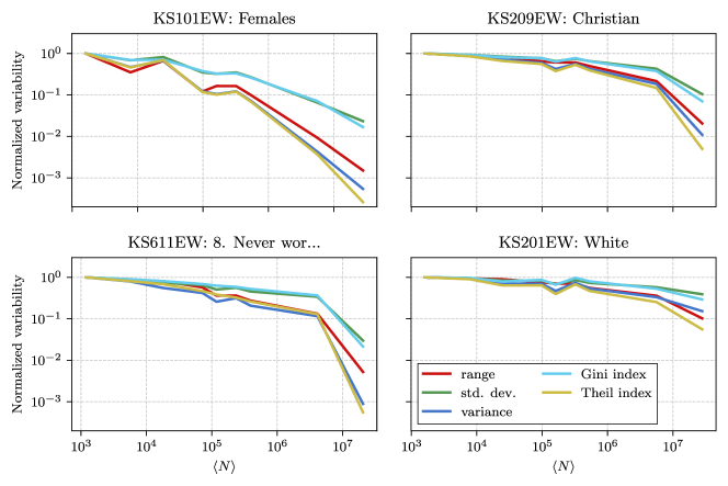
Figure 1: Normalized variability (colored curves) of four different demographic categorizations across different hierarchical scales.

As can be seen in Fig. 1, all of the considered variability measures exhibit the same qualitative behavior: they decay as the scales become coarser. Some of the measures decay faster than others, but in general, the measures either scale together with the standard deviation or with the variance, which indicates that different scaling behavior in measures is just a matter of units. Therefore, further in this paper we will consider only standard deviation as the measure of variability (heterogeneity).

Comparison across the different demographic categorizations yields desired qualitative insights: in some cases normalized variability decays faster than in others. The faster decay indicates that the population becomes more uniform faster, which is expected if the population is not segregated with respect to that categorization. There is little evidence for segregation based on sex, but on the other hand, religious, ethnic, and economic segregation is a well–documented phenomenon [9].

3 Baseline null model

To provide a baseline for the understanding of the randomness in the observed demographic heterogeneity let us introduce a null model. The core idea of the null model would be to remove any spatial or hierarchical associations present in the empirical data.

To this end, the input of the null model is the data from the finest scale and the desired number of units at a coarser scale. The finest scale units are randomly assigned to groups, the number of which is equal to the desired number of units at the coarser scale. Random assignment happens with one important restriction: the groups need to have as similar number of units assigned to them as possible. Units within the groups are then combined to produce the randomized coarser scale units. To avoid Simpson’s paradox, we add the raw numbers $X_{i}^{\left(k\right)}$ instead of simply averaging the fractions $x_{i}^{\left(k\right)}$. Repeating these steps for all coarser scales allows us to see how fast the normalized variability decays if the process is purely random.

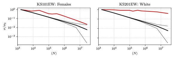
Figure 2: Normalized standard deviation of the two different demographic categorizations across the different scales: empirical data (red curve) compared against the null model (median is shown as solid black curve, while $95\%$ confidence interval is limited by the thin dashed black curves).

As can be seen in Fig. 2, both sex and race curves show higher variability than would be expected if the migration and demographic change were a random processes (the empirical curves are above the null model curve). Notably, the null model in both cases produces power–law scaling behavior

$$\frac{\sigma}{\sigma_{0}}\sim\frac{1}{\sqrt{\left\langle N\right\rangle}}.$$ (2)

Such scaling relationship is expected, as when increasing the scale we are effectively averaging values on the lowest scale. Then the variance of the mean of $N$ random values $\bar{x}=\frac{1}{N}\sum_{i=1}^{N}x_{i}$ would be given by:

$$\mathrm{Var}\left[\bar{x}\right] =\mathbb{E}\left[\left(\bar{x}-\mathbb{E}\left[\bar{x}\right]\right)^{2}\right]=\mathbb{E}\left[\left(\frac{1}{N}\sum_{i=1}^{N}x_{i}-\mathbb{E}\left[\frac{1}{N}\sum_{i=1}^{N}x_{i}\right]\right)^{2}\right]=\frac{1}{N^{2}}\mathbb{E}\left[\left(\sum_{i=1}^{N}x_{i}-\mathbb{E}\left[\sum_{i=1}^{N}x_{i}\right]\right)^{2}\right]=$$

$$=\frac{1}{N^{2}}\mathrm{Var}\left[\sum_{i=1}^{N}x_{i}\right]=\frac{1}{N^{2}}\left\{\sum_{i=1}^{N}\mathrm{Var}\left[x_{i}\right]+\sum_{i=1}^{N}\sum_{j=1}^{N}\mathrm{Cov}\left(x_{i},x_{j}\right)\right\}.$$ (3)

For the independent random values $x_{i}$, with $\mathrm{Cov}\left(x_{i},x_{j}\right)=0$, we have:

$$\sigma=\sqrt{\mathrm{Var}\left[\bar{x}\right]}=\sqrt{\frac{1}{N}\mathrm{Var}\left[x_{i}\right]}=\frac{\sigma_{0}}{\sqrt{N}}.$$ (4)

This relationship will hold for any underlying distribution of the random values on the lowest scale. Though, in the empirical data we would expect that these values would follow Beta distribution or a mixture of Beta distributions [7]. In Figs. 1 and 2 we have $\left\langle N\right\rangle$ as independent variable, because in the empirical data set higher hierarchical scales are produced by combining not necessarily the same number of smaller units.

For the ethnic data, finding the slower decay of variability (in comparison to the null model) was expected. But for the sex data, the obtained slower decay is unexpected, though the difference from the null model is relatively small. The deviations in the latter case could likely be explained by the data anonymization procedures and the presence of institutional installations favoring one of the sexes (e.g., military bases, convents).

4 Non–monotonicity of variability

Note that the empirical curves in Figs. 1 and 2 are non–monotonic, while the intuition from the baseline null model would suggest that the variability measures should monotonically decrease with coarser scales. The non–monotonicity cannot be explained by the objective socio–demographic mechanisms such as segregation, but instead can be replicated by assuming that it is an observational effect. Namely, non–monotonicity can be replicated if we allow for the hierarchical associations to be imperfect: meaning that the coarser scale units are not necessarily produced by combining the finer scale units. For example, some finer scale units might be split and then be incorporated into different coarser scale units. If this is allowed then the variability will decay non–monotonically.

To verify this intuition by numerical simulation, let us generate a random grid with $256\times 256$ cells. Let each cell, with equal probability, contain either a value of $0$ or a value of $1$. Then, let us measure the variability of such grid at different scales (up to $4\times 4$ grid, meaning that the cells at the coarsest scale are $64\times 64$ in size). If the cells are combined consistently (without splitting finer scale units), then the obtained curve is monotonic (the red curve in Fig. 3). On the other hand, if the cells are combined inconsistently (i.e., allowing the splits), then the non–monotonicity can be observed (the green curve in Fig. 3).

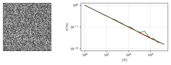
Figure 3: Random grid (left) and normalized standard deviation curve (right) measured across the consistent (red curve) and inconsistent hierarchical scales (green curve). Thin black dashed curve shows Eq. (2).

5 Modeling (anti–)segregation

One of the simplest models for segregation would be to split the grid into regions with different probabilities for a cell on a grid to contain $0$ or $1$, thus artificially creating spatial divisions. One such grid of size $256\times 256$ is shown in Fig. 4. It was obtained with $p_{1}=0.6$ in two $128x128$ regions (these regions appear darker in the figure), and symmetrically $p_{1}=0.4$ in the other two $128\times 128$ regions (these appear lighter). The corresponding normalized standard deviation curve (also shown in Fig. 4) indicates that at the lowest scales the heterogeneity (as measured by standard deviation) scales consistently with the random model. Saturation at the higher scales is induced by the way we have introduced segregation.

Figure 4: Segregated random grid (left) and normalized standard deviation curve (right) measured across the consistent scales (red curve). Thin black dashed curve shows Eq. (2).

Notably, the empirical normalized standard deviation curves have slightly different shape than predicted by the segregated random grid model. Namely, the empirical curves exhibit slower decay of heterogeneity at the lowest scales, with the decay of the curves becoming faster as the scale increases. This shape can be qualitatively replicated by Schelling’s segregation model [10] (see Fig. 5), or the Kawasaki–Ising model [11, 12] (see Fig. 6). While the classic formulation of the Schelling’s segregation model doesn’t exhibit anti–segregation regime (though it can be easily modified to do so), but anti–segregation regime can be found in the Kawasaki–Ising model with anti–ferromagnetic interactions. Both models were simulated on $128\times 128$ grid, being initialized with a random configuration with a constraint that there should be the same number of cells containing $0$ and $1$ ($16\%$ of cells were empty in simulations with the Schelling’s model). In both cases the state was observed after $10^{7}$ Monte Carlo steps.

Figure 5: Normalized standard deviation curves obtained for the Schelling’s model with different happiness thresholds: $0$ (red curve), $25\%$ (green), $37.5\%$ (blue), and $50\%$ (cyan). All of the obtained curves are above or overlap the thin black dashed curve, which corresponds to the random grid model.

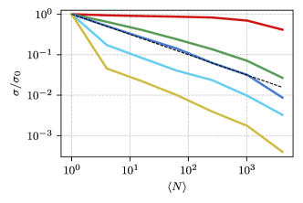
Figure 6: Normalized standard deviation curves obtained for the Kawasaki–Ising model. The curves above or overlapping the thin black dashed curve (corresponding to the random grid model) were obtained in ferromagnetic regime for different inverse temperatures: $\beta=2$ (red curve), $1$ (green), $0.1$ (blue). The curves below were obtained in anti–ferromagnetic regime for $\beta=2$ (cyan), $4$ (yellow).

6 Conclusions

Here we have explored scaling of variability measures in hierarchical demographic data. From the empirical point-of-view we have examined United Kingdom 2011 data set. We have considered five different variability measures, and found that they mostly exhibit the same qualitative behavior. Therefore to carry out the analysis choosing either one of them would be sufficient. While the range is the easiest variability measure to calculate, it is highly sensitive to outliers, thus it is less suitable than the variance or the standard deviation. On the other hand Gini and Theil indices require more computational effort to calculate than the variance or the standard deviation. As the standard deviation has the same units as the quantity it is calculated from, we prefer it over the variance.

In the empirical analysis we have observed non–monotonicity of the normalized variability curves, but as all the measures produce qualitatively the same non–monotonic behavior, we are prompted to look at other observational imperfections. We were able to reproduce the non–monotonicity by assuming that hierarchical relationships are imperfect: that some of the smallest scale units are getting split when producing higher scale units.

Finally, we have shown that the obtained empirical curves cannot be well explained by artificially introducing segregation into the random grid model. Instead a bit more complicated model, such as the Schelling’s segregation model or the Kawasaki–Ising model are necessary to reproduce qualitative behavior of the empirical curves.

In the foreseeable future we expect to use this preliminary analysis as a basis of producing hierarchical correlation index similar in purpose to the spatial correlation indices. And to further enhance spatial models of opinion dynamics (such as [7]).

Author contributions

AK: Conceptualization, Methodology, Software, Writing, Visualization. JK: Conceptualization, Methodology.

References

- [1] C. Castellano, S. Fortunato, V. Loreto, Statistical physics of social dynamics, Reviews of Modern Physics 81 (2009) 591–646. arXiv:0710.3256, doi:10.1103/RevModPhys.81.591.
- [2] J. Fernandez-Gracia, K. Suchecki, J. J. Ramasco, M. San Miguel, V. M. Eguiluz, Is the voter model a model for voters?, Physical Review Letters 112 (2014) 158701. arXiv:1309.1131, doi:10.1103/PhysRevLett.112.158701.
- [3] F. Vazquez, Modeling and analysis of social phenomena: Challenges and possible research directions, Entropy 24 (4) (2022) 491. doi:10.3390/e24040491.
- [4] F. Sano, M. Hisakado, S. Mori, Mean field voter model of election to the house of representatives in Japan, in: JPS Conference Proceedings, Vol. 16, The Physical Society of Japan, 2017, p. 011016. arXiv:1702.03603, doi:10.7566/JPSCP.16.011016.
- [5] A. Kononovicius, Empirical analysis and agent-based modeling of Lithuanian parliamentary elections, Complexity 2017 (2017) 7354642. arXiv:1704.02101, doi:10.1155/2017/7354642.
- [6] D. Braha, M. A. M. de Aguiar, Voting contagion: Modeling and analysis of a century of U.S. presidential elections, PLOS ONE 12 (2017) e0177970. doi:10.1371/journal.pone.0177970.
- [7] A. Kononovicius, Compartmental voter model, Journal of Statistical Mechanics 2019 (2019) 103402. arXiv:1906.01842, doi:10.1088/1742-5468/ab409b.
- [8] A. D. Cliff, J. K. Ord, Spatial Processes: Models and Applications, Pion, 1981.
- [9] M. Oka, D. W. S. Wong, Segregation: A multi-contextual and multi-faceted phenomenon in stratified societies, in: Handbook of Urban Geography, Edward Elgar Publishing, 2019, pp. 255–280. doi:10.4337/9781785364600.00028.
- [10] E. Hatna, I. Benenson, The Schelling model of ethnic residential dynamics: Beyond the integrated - segregated dichotomy of patterns, Journal of Artificial Societies and Social Simulation 15 (2012) 6. doi:10.18564/jasss.1873.
- [11] K. Kawasaki, Diffusion constants near the critical point for time-dependent Ising models. I, Physical Review 145 (1966) 224–230. doi:10.1103/PhysRev.145.224.
- [12] K. Kawasaki, Diffusion constants near the critical point for time-dependent Ising models. II, Physical Review 148 (1966) 375–381. doi:10.1103/PhysRev.148.375.